Embed Size (px)
Citation preview
In-Cycle Control of the Thermoforming Reheat Process
by
Ben Moore
Department of Electrical and Computer Engineering
McGill University
A THESIS SUBMITTED TO THE FACULTY OF GRADUATE STUDIES AND RESEARCH IN PARTIAL FULFILLMENT OF THE
REQUIREMENTS OF THE DEGREE OF
Masters in Engineering
May 2002
i
Abstract
In this thesis, the problem of closed loop control during the thermoforming
sheet reheat process is considered. The approach aims to improve the material
distribution of a formed thermoplastic part via better sheet temperature control
prior to forming. Improved control of material distribution will increase part
quality and result in fewer part rejects, thereby increasing production efficiency.
A process model consisting of individual components describing sensor,
heater, and sheet heating dynamics has been developed. Recommendations for
improvements to the process model, particularly for the sheet heating model, are
also made. An in-cycle control strategy is proposed and the feasibility of in-cycle
sheet reheat temperature control is examined based on simulation results for
multivariable H∞ control is examined based on simulation results for
multivariable H∞ and MPC controller designs.
ii
Résumé
Cette dissertation traite du problème de commande rétroactive du procédé
de chauffe d'une feuille de polymère pour le thermoformage. Notre approche a
pour but d'améliorer la distribution de matière dans une pièce formée en
thermoplastique à l'aide d'une meilleure commande de température de la feuille
avant l'opération de formage. Une meilleure distribution de masse sur la pièce
finie améliore sa qualité et permet de diminuer le nombre de pièces rejetées, ce
qui augmente la productivité.
On développe un modèle du procédé composé de modèles du capteur, du
système de chauffage par radiation, et de la dynamique de chauffe de la feuille.
On donne des recommandations pour l'amélioration du modèle du procédé, en
particulier pour le modèle de température de la feuille. Une stratégie de
commande en-cycle est proposée, et la faisabilité d'une commande de température
de la feuille est examinée sur la base de résultats de simulation de compensateurs
multivariables (H-infinity) et à commande prédictive (MPC).
iii
Contents List of Tables List of Figures List of Symbols 1. Introduction 2. Process Description
2.1. Introduction and Historical Review 2.1.1. Advantages and Disadvantages 2.1.2. Parts Made by Thermoforming
2.2. Physical Description of the Process 2.2.1. Components of Thermoforming
2.2.1.1. Sheets 2.2.1.2. Clamping Mechanisms 2.2.1.3. Heating Systems 2.2.1.4. Process Controls 2.2.1.5. Molds
2.2.2. Thermoforming Machines 2.2.2.1. Sheet Fed 2.2.2.2. Roll Fed
2.2.3. Process Steps 2.2.3.1. Sheet Handling 2.2.3.2. Sheet Heating 2.2.3.3. Forming 2.2.3.4. Cooling 2.2.3.5. Trimming
2.3. IMI Equipment Description 3. Process Modeling
3.1. Introduction 3.2. Sensors
3.2.1. Thermoforming Instrumentation 3.2.2. Sensor Modeling 3.2.3. Calibration and Maintenance
3.3. Heater Modeling 3.3.1. Disturbances and Modeling Errors 3.3.2. Model Validation 3.3.3. Additional Heater Dynamics
3.4. Sheet Modeling 3.4.1. Heat Transfer Theory 3.4.2. Sheet Model
3.4.2.1. Modeling Equations For a Single Sheet Zone
v
v
vii
1
8 8
10 11 12 13 13 18 18 20 21 24 24 25 25 25 26 29 29 29 30
33 33 42 43 45 45 47 54 55 56 59 60 66 68
iv
3.4.2.2. Model Validation 3.4.2.3. Disturbances 3.4.2.4. Future Modeling Improvements
4. Controller Development
4.1. Introduction 4.2. H∞ Optimal Controller Design
4.2.1. H∞ Optimal Control Theory 4.2.2. H∞ Controller Design 4.2.3. Simulation Results 4.2.4. Stability Analysis
4.3. MPC Design 4.3.1. Introduction 4.3.2. MPC Controller Design 4.3.3. Simulation Results
4.4. Comparison Between Designs
5. Summary and Concusions Acknowledgements Bibliography Appendix
70 73 74
75 75 77 77 83 93 97 99 99
100 106 110
112
114
115
117
v
List of Tables
2.1 list of products made by thermoforming 2.2 types of themoplastic sheets used for thermoforming 2.3 electrical heater types 2.4 IMI AAA thermoforming machine data 3.1 comparision between modeling approaches 3.2 IR sensor cost comparisions 4.1 H∞ design performance weighting functions 4.2 signal definitions for H∞ control design 4.3 block definitions for H∞ controller design 4.4 parameter uncertainty levels for sheet heating model
11 17 20 32
35 45
83 85 85 87
List of Figures
2.1 historical timeline of themoforming industry 2.2a basic femal mold 2.2b material distribution for female molded part 2.3a basic male mold 2.3b material distribution for male molded part 2.4 basic single station shuttle machine 2.5 example sheet heating profile with forming window 2.6 example sheet heating profile: temperature gradient through sheet
thickness 2.7 oven layout for IMI thermoforming machine 2.8 simplified control circuit diagram for heater zone B1 3.1 black box modeling configuration 3.2 response for a step from 350 to 400 oC on heater zone B2 3.3 effects on bottom sheet surface temperature response due to different
input step magnitudes for heater zone B2 3.4 effects on bottom sheet surface temperature response due to different
input step times for heater zone B2 3.5 response for a step from 350 to 400 oC on heater zone B2 3.6 bottom sheet surface temperature response for step inputs on heater
zones B2 and B5 3.7 individual system components 3.8 sample heater step response 3.9 physical dimensions of heating elements 3.10 configuration of heater model 3.11 heater embedded to surface temperature offset 3.12 temperature dependency of embedded heater step response 3.13 temperature dependant time constant for first order embedded heater
model
10 22 22 23 25 25 27 28
31 32
36 38 39
39
40 40
42 48 48 49 50 52 52
vi
3.14 model validation results for heater zone T2 3.15 model validation results for heater zone B2 3.16 heater settling time 3.17 heater zone coupling 3.18 negative step response of second order surface model with actual
experimental data as input 3.19 negative step response of first order embedded model with actual
experimental data as input 3.20 conceptual block diagram for sheet heating model 3.21 coordinate system and direction of energy transfer 3.22 discretization of sheet into isothermal zones 3.23 sheet discretiaztion: node numbers 3.24 simulated temperature distribution through the sheet at various time
instants 3.25 parameter estimation results from unconstrained least squares
algorithm 3.26 manual tuning parameter estimation results 4.1 ideal sheet surface temperature setpoint trajectory 4.2 basic LFT notation for H∞ control design 4.3 additive uncertainty 4.4 output multiplicative uncertainty 4.5 LFT uncertainty structure 4.6 mixed-sensitivity H∞ design structure 4.7 H∞ controller design interconnection 4.8 H∞ multiplicative uncertainty results 4.9 desired shape of control moves weighting function 4.10 long-cycle H∞ simulation results: sheet surface temperatures 4.11a short-cycle H∞ simulation results: sheet surface temperatures 4.11b short-cycle H∞ simulation results: error signal and control moves 4.12 long-cycle H∞ simulation results with aggressive controller design 4.13 long-cycle H∞ simulation results for full order controller 4.14 mixed-sensitivity closed loop µ results for short-cycle controller
design 4.15 closed loop µ results for short-cycle controller design: no
performance specifications 4.16 long-cycle MPC simulation results: sheet surface temperatures 4.17a short-cycle MPC simulation results: sheet surface temperatures 4.17b short-cycle MPC simulation results: error and control moves 4.18 long-cycle MPC simulation results for full order controller
56 56 57 58 59
59
60 60 67 68 70
72
73
76 78 80 81 81 83 84 89 92 94 95 95 96 97 98
98
107 108 108 109
vii
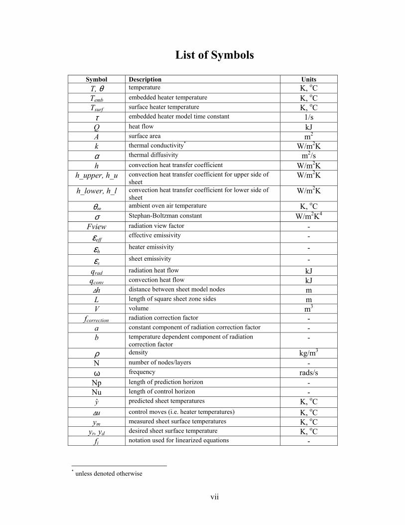
List of Symbols
Symbol Description Units T, θ temperature K, oC Temb embedded heater temperature K, oC Tsurf surface heater temperature K, oC
τ embedded heater model time constant 1/s Q heat flow kJ A surface area m2 k thermal conductivity* W/m2K α thermal diffusivity m2/s h convection heat transfer coefficient W/m2K
h_upper, h_u convection heat transfer coefficient for upper side of sheet
W/m2K
h_lower, h_l convection heat transfer coefficient for lower side of sheet
W/m2K
θ∞ ambient oven air temperature K, oC σ Stephan-Boltzman constant W/m2K4
Fview radiation view factor - εeff effective emissivity -
εh heater emissivity -
εs sheet emissivity - qrad radiation heat flow kJ qconv convection heat flow kJ
∆h distance between sheet model nodes m L length of square sheet zone sides m V volume m3
fcorrection radiation correction factor - a constant component of radiation correction factor - b temperature dependent component of radiation
correction factor -
ρ density kg/m3
N number of nodes/layers - ω frequency rads/s
Np length of prediction horizon - Nu length of control horizon - y predicted sheet temperatures K, oC
∆u control moves (i.e. heater temperatures) K, oC ym measured sheet surface temperatures K, oC
yr, yd desired sheet surface temperature K, oC fi notation used for linearized equations -
* unless denoted otherwise
1
1. Introduction
Thermoforming is a process in which useful tub-shaped plastic parts are
manufactured from a flat sheet of plastic material. The thermoforming process is
composed of three basic phases: 1) sheet heating, 2) forming, and 3) cooling. In the first
stage a flat plastic sheet is heated in an oven until the material is soft and pliable. The
sheet is then formed to a mold using pressure and/or vacuum forces in order to achieve
the desired part shape. Finally, the formed part is left to cool in the mold until the
material solidifies and is rigid enough to be removed from the mold.
This thesis focuses only on the details of the heating stage, which is often referred
to as sheet reheat in industry. The goal of the research is to develop a control strategy
that is capable of tracking desired sheet temperature profiles throughout the reheat cycle.
The sheet temperature is altered by manipulating the temperatures of heating elements
within the oven. Proper control of sheet temperature will allow for an overall
improvement of the thermoforming process. The specific objectives of a control system
for thermoforming reheat are defined by considering the motivations for process
improvement. The most basic motivation is improved part quality. Higher quality parts
can be achieved through better control of material distribution before the actual forming
of the sheet via close control of sheet temperature distribution. Close temperature control
and disturbance rejection will also result in a reduction in the number of rejected parts for
a given production cycle. As a result, production efficiency will increase and material
costs can significantly decrease. This is particularly important for producers of products
manufactured from very expensive plastic materials.
Production efficiency can also be improved by decreasing the time it takes to
make each individual part. Control during sheet reheat will allow for more aggressive
sheet temperature trajectories, and thus shorter heating times for some thermoforming
operations. In other words, control during the reheat stage can lead to an increase in
production rates.
It is also possible for reheat temperature control to result in a decrease in energy
consumption by generating optimal (in terms of energy) control signals that will achieve
the desired sheet temperature profile. This should be a significant motivation for the
2
application of sheet reheat control since thermoforming is generally an energy intensive
process. Energy, or heating, costs are often the most significant operating expenses for a
thermoforming operation.
Finally, control of sheet reheat can potentially result in reduced machine
maintenance. As the oven heating elements age, their performance can deteriorate. Also,
individual heating elements can deteriorate at different rates. This results in non-uniform
sheet heating which can subsequently affect part quality. A control system can
effectively extend the life of heating elements by compensating for uneven sheet heating.
The end result is an increase in production efficiency over time.
There are two opportunities to take corrective control action for the
thermoforming reheat process: in-cycle, and cycle-to-cycle. A cycle-to-cycle control
strategy involves updating heater temperature settings at the end of each reheat cycle
such that the next part that is made is improved in some sense. The role of cycle-to-cycle
control is to iteratively improve part quality via better sheet temperature distribution and
to correct for gradual drift of machine operating parameters. An in-cycle control strategy
involves manipulating heater temperatures during the actual heating of the sheet. The
role of in-cycle control is to provide corrective action for the purposes of reference
trajectory tracking and short-term disturbance rejection.
The in-cycle control problem is the subject of this thesis. Although it appears to
be quite a simple process, in-cycle sheet temperature control of the thermoforming reheat
process is a very challenging control problem in which a number of factors contribute to
the overall difficulty of the problem. First, the thermoforming reheat process is highly
nonlinear and time-varying. Second, thermoforming reheat is a distributed parameter
system governed by a set of partial differential equations, not ordinary differential
equations. Control during sheet reheat is also complicated by the fact that there is a high
level of uncertainty surrounding the process, particularly with the material properties.
The fact that this is a multi-input, multi-output (MIMO) problem with a high degree of
coupling between inputs and outputs also introduces additional complexity. Finally,
there are a number of hard constraints that must be taken into consideration such as
maximum allowable sheet and heater temperatures.
3
Another factor that contributes to the overall difficulty in developing an effective
in-cycle control strategy for the thermoforming reheat process is the overwhelming lack
of information on closed-loop control of thermoforming available in the literature. In
fact, not a single article specifically addressing in-cycle control of thermoforming reheat
could be found; however, one paper by Michaeli and van Marwick, [16], was found.
They proposed ideas for a closed-loop cycle-to-cycle control strategy as well as
techniques for online measurement of part wall thickness.
The fact that there has been very little work done on the in-cycle control of the
thermoforming reheat process is a direct result of the historical conservative nature of the
thermoforming industry. In comparison, much more work on process modeling and
control has been done for blow molding, and in particular, injection molding. Simulation
software has long been used to improve and speed up the development of injection
molded parts. Advanced model based control techniques, such as the work done by
Dubay in [17], have also been used to improve the injection molding process. In a
similar work, DiRaddo and Garcia-Rejon, [25], demonstrate the effectiveness of in-cycle
control of extrusion blow molding.
The thermoforming industry is, however, catching up. Although the application
of closed-loop control is not yet established, the use of thermoforming simulation
software during product design is increasing. A number of simulation packages are now
commercially available. T-Sim from Accuform is recognized as one of the first
simulation packages available to thermoformers. C-Mold, which offers the popular
Moldflow injection molding simulation software, also has a thermoforming simulation
package. Other simulation packages are offered by Fluent Inc. and ESI Group.
Sherwood Technologies is in the process of developing Java based programs for the
simulation of sheet heating and cooling only. Finally, IMI’s FormSim software package
allows users to simulate the various stages of the thermoforming process.
As the demand for thermoforming simulation software increases, so too will the
demand for increased accuracy of the simulated predictions. The work of Yousefi et al.
in [15] addresses the issues related to the improvement of sheet temperature prediction
during the sheet reheat stage. The approach aims to improve the quality of predictions
through more accurate evaluation of simulation input parameters. Results indicate that
4
prediction accuracy can be greatly improved by using more accurate1, and in some cases,
time-varying model parameters. Continued improvements in thermoforming simulation
modeling will only help to increase the effectiveness of future closed-loop control
strategies that may be applied to improve the thermoforming process. Modeling
improvements will also improve the effectiveness of open-loop control strategies such as
the strategy presented in [24] by Alaeddine and Doumanidis, which involves the solution
of the inverse heat conduction problem.
Fortunately, the application of advanced model based control strategies to similar
thermal processes are quite well documented in the literature, and the information that is
available can be adapted to the thermoforming reheat process.
The manufacturing of advanced engineering materials through the used of multi-
zone furnaces is one such similar process. In [11], Gopinathan et al. discuss the
modeling and control of hot isostatic pressing (HIP) furnaces used for the processing of
advanced aerospace materials. The authors demonstrate the effectiveness of a fault
tolerant model predictive control (MPC) design and stress its superiority over existing
PID control of HIP furnaces. A projective control design for a multi-zone crystal growth
furnace was developed by Srinivasan et al. in [21]. The projective controller has a
structure similar to a MIMO proportional-plus-integral controller, and it exhibits
reasonable transient behavior and good steady state error performance. The authors
indicate that the projective control approach is particularly appealing for furnaces having
a large number of heating zones because the projective control approach allows for the
systematic increase in controller order until the desired performance criteria are satisfied,
thus yielding a satisfactory controller of minimal complexity.
Rapid thermal processing (RTP) of semiconductor materials is another thermal
process that is very similar to thermoforming reheat. RTP involves the heating of
semiconductor wafers via high temperature radiation heating lamps. Strict wafer
temperature control is the determining factor in achieving desired material properties. A
significant amount of work has been done on the modeling and control of RTP systems.
1 More accurate model parameters were determined via a series of identification experiments.
5
Cho and Kailath, in [14], compare black box and first principles modeling
approaches for RTP systems. In [23], Lee et al. propose a robust controller design for an
RTP system using the structured uncertainty approach. A model based feed-forward,
feedback controller structure with gain scheduling is presented in [13] by Park et al.
Similarly, Kamali and Kosut, in [19], present a time-varying feed-forward, feedback
control design. The authors state that due to the time-varying nature of the linearized
model around a reference trajectory, a time-varying LQR design is superior to controller
designs with constant parameters. It is important to mention, however, that the
performance of this design was evaluated based on single-input, single-output (SISO)
simulations. The development of a time-varying MIMO controller is a much more
difficult problem.
MPC designs have also been proposed for RTP systems. In [20], Dekeyser and
Donald III document the successful application of an MPC design to an actual RTP
system. The model used for the prediction of wafer temperatures consisted of a number
of locally linearized models that describe the RTP reactor over its entire operating range.
A fuzzy logic based combination of the individual linear model outputs led to the actual
nonlinear model output used in the prediction strategy.
In [12], Schaper et al. used a multivariable internal model control (IMC) approach
to improve the uniformity and repeatability of wafer temperatures in RTP systems. The
authors also address a number of practical controller implementation issues. Their goal
was to design a generalized control strategy that could be applied to any RTP machinery,
and therefore, allow for flexible manufacturing.
It was mentioned earlier that efforts are being made to improve the accuracy of
thermoforming simulation predictions. Even with accurate predictions, complex
simulation software has the drawback of being just that, complex. The software uses
large time dependant and often three-dimensional finite element models for the prediction
of sheet temperatures. Even when run on high performance computers, simulations can
take hours, even days, to execute. Regardless of accuracy, this makes these large finite
element models virtually useless for real-time applications. A great deal of research work
has been done recently on the reduction of large simulation models. It is worthwhile to
6
briefly discuss the details of one of the more popular model reduction techniques as well
as potential uses for reduced order models.
Banerjee et al., in [18], discuss the proper orthogonal decomposition (POD)
model reduction approach for RTP systems. The modeling equations are solved by the
Galerkin finite element method, which approximates the temperature fields by using
expansions in piecewise, low order polynomials. This approach has the advantage of
being general and flexible, but the large number of coefficients required leads to large
nonlinear matrix problems. The number of coefficients could be reduced, in principle, if
the approximating functions were similar in form to the actual solution. One approach
for obtaining better approximating functions is the POD method, which involves
obtaining empirical eigenfunctions from experimental data or detailed model predictions
of temperature fields, or snapshots, for the entire RTP reactor at discrete time intervals.
The eigenfunctions then form an optimal basis set for the given series of snapshots. The
eigenfunctions can be viewed as a set of ideal fitting functions. The actual model
reduction is achieved by considering only a few dominant eigenfunctions that describe
most of the temperature field data.
The result is a nonlinear, low order model that is obtained without approximating
the physical equations that govern the process. These equations are therefore more
accurate over a wider range of conditions as compared to conventional reduced order,
linearized models. An order of magnitude reduction in simulation execution time was
achieved with the reduced order model as compared to the full order finite element RTP
model. The authors suggest that a well designed reduced order model could help in
cutting down the number of experiments required in designing a process recipe and thus
reduce the transition time in bringing a process from the research to the manufacturing
stage. It is also suggested that a reduced order POD model could be used in real-time,
advanced model based control strategies. A reduced order POD model could potentially
be obtained from thermoforming simulation software and used to predict sheet
temperatures in an MPC controller design.
A brief description of thermoforming, as well as a problem definition, was given
in this section. A summary of relevant work in the literature was also presented. A more

7
detailed description of the thermoforming process is given in Section 2. Section 3 details
the development of the process models used for controller design. The controller design
and simulation results are given in Section 4. A summary and conclusion are given in
Section 5.
8
2. Process Description
2.1 Introduction and Historical Review
Thermoforming is a generic term used to categorize the many different techniques
for producing useful articles from a flat thermoplastic sheet. The name thermoforming
suggests the application of heat. Although this is generally true, there are specialized
forming techniques that do not require heat; however, for simplicity, the application of
heat will be assumed throughout the remainder of this discussion. The idea behind the
thermoforming process is not new. Even early man used heat to shape various organic
materials into useful tools. Nevertheless, the real roots of thermoforming came with the
development of synthetic rubber during WWII. Various thermoplastic materials soon
followed and subsequently the thermoforming industry was born. The commercial
success of thermoforming began in the late 1940’s and early 50’s with the development
of the packaging industry. By the 60’s blister packaging developed into a high volume
market. The 60’s also saw new advancements and trends in the industry as well as the
establishment of separate thin and thick sheet sectors. During this time resin
manufactures became more involved and offered technical support and expert knowledge
of material properties to thermoformers. By the 70’s thermoforming machine
manufacturers also began to support the advancement of thermoforming technology.
Demand had risen significantly in a few short years, which prompted machine
manufacturers to develop high output equipment. As the production volume increased in
many thermoforming operations, the desire to cut costs prompted machine manufacturers
to make advancements in production and quality controls which led to more automated
operations. The desire to stay competitive and decrease costs also prompted
improvements in scrap handling. Minimization of material costs and recycling suddenly
became important issues. The 80’s saw an even greater demand for more cost effective,
automated operations. This led to further advancements in thermoforming technology
and allowed thermoformers to introduce new product lines that were previously not
possible. The 80’s also saw the introduction of new pellet-to-product equipment as well
as major advancements in process controls. The advancement of thermoforming
9
technology has not been continuous however. The industry saw a significant slowdown
in the early 90’s as a result of the economic slowdown in North America as well as the
repercussions of rising environmental concerns, which led to many fast food
organizations discontinuing the use of certain types of takeout food containers. As a
result, some product lines were discontinued and many thermoforming operations were
left idle and a good number had to shut down completely.
Today, the thermoforming industry is seeing growth once again. The relatively
low capital costs associated with the thermoforming process has spurred interest in the
possibility that advances in technology may allow new thermoforming techniques to
produce many common parts traditionally manufactured by other more expensive
processes.
Although many advancements have been made since thermoforming’s early
years, the industry, as a whole, has been relatively conservative in terms of the
application of new technologies when compared to other polymer processing industries.
For example, the injection molding industry has long used established FEM simulation
software in the design and production of new parts. Because thermoforming is still
considered to be a process of high craftsmanship and experience, it is regarded as the
polymer processing area with the highest growth potential. Advances in materials and
process controls (specifically for sheet heating) will allow more complex parts to be
made. For example, twin-sheet thermoforming is now becoming the process of choice
for manufacturing gas tanks that meet the strict Partial Zero Emissions Vehicle (PZEV)
mandates that have been introduced recently in California. Also, it has been suggested
that the forming of very strong, lightweight foamed material will continue to increase.
As was the case with injection molding, thermoforming will likely see more automation
and shorter product development times with the aid of various CAE tools. As heating
costs continue to rise it is reasonable to believe that strides will be taken towards
improved, energy efficient thermoforming processing. Similarly, rises in material costs
will see a continued effort to reduce the amount of waste associated with thermoforming.
No one can say for certain exactly where the thermoforming industry will be 10 years
from now; however, one can be confident in saying that the future definitely looks quite
10
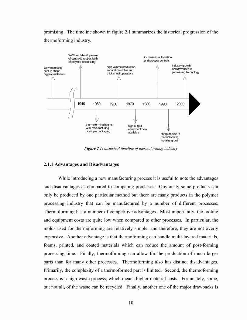
promising. The timeline shown in figure 2.1 summarizes the historical progression of the
thermoforming industry.
1940 1950 1960 1970 1980 1990 2000
early man uses heat to shape organic materials
WWII and developementof synthetic rubber, birthof polymer processing
high volume production,separation of thin andthick sheet operations
increase in automationand process controls
industry growthand advances in processing technology
high outputequipment nowavailable sharp decline in
thermoformingindustry growth
thermoforming beginswith manufacturingof simple packaging
Figure 2.1: historical timeline of thermoforming industry
2.1.1 Advantages and Disadvantages
While introducing a new manufacturing process it is useful to note the advantages
and disadvantages as compared to competing processes. Obviously some products can
only be produced by one particular method but there are many products in the polymer
processing industry that can be manufactured by a number of different processes.
Thermoforming has a number of competitive advantages. Most importantly, the tooling
and equipment costs are quite low when compared to other processes. In particular, the
molds used for thermoforming are relatively simple, and therefore, they are not overly
expensive. Another advantage is that thermoforming can handle multi-layered materials,
foams, printed, and coated materials which can reduce the amount of post-forming
processing time. Finally, thermoforming can allow for the production of much larger
parts than for many other processes. Thermoforming also has distinct disadvantages.
Primarily, the complexity of a thermoformed part is limited. Second, the thermoforming
process is a high waste process, which means higher material costs. Fortunately, some,
but not all, of the waste can be recycled. Finally, another one of the major drawbacks is
11
the fact that only certain materials can be used with the thermoforming process. This last
point will be elaborated on in the discussions to follow.
2.1.2 Parts Made by Thermoforming
Early on, the thermoforming industry was dominated by the production of very
simple tub-shaped parts for the packaging industry. Today, numerous different parts of
varying complexity are produced using thermoforming techniques. Many thermoformed
parts that are in use today have been made to replace earlier forms of the same products
that were made from different materials. Usually, plastic is much more durable, or it has
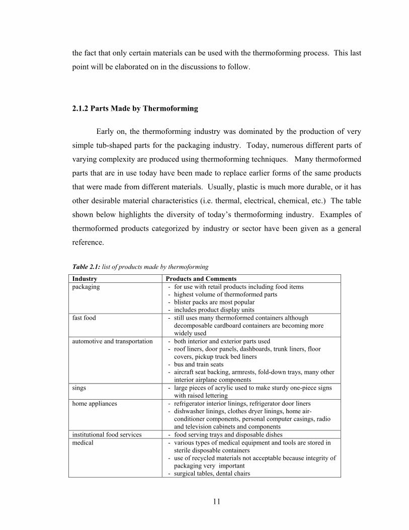
other desirable material characteristics (i.e. thermal, electrical, chemical, etc.) The table
shown below highlights the diversity of today’s thermoforming industry. Examples of
thermoformed products categorized by industry or sector have been given as a general
reference.
Table 2.1: list of products made by thermoforming
Industry Products and Comments packaging - for use with retail products including food items
- highest volume of thermoformed parts - blister packs are most popular - includes product display units
fast food - still uses many thermoformed containers although decomposable cardboard containers are becoming more widely used
automotive and transportation - both interior and exterior parts used - roof liners, door panels, dashboards, trunk liners, floor
covers, pickup truck bed liners - bus and train seats - aircraft seat backing, armrests, fold-down trays, many other
interior airplane components sings - large pieces of acrylic used to make sturdy one-piece signs
with raised lettering home appliances - refrigerator interior linings, refrigerator door liners
- dishwasher linings, clothes dryer linings, home air-conditioner components, personal computer casings, radio and television cabinets and components
institutional food services - food serving trays and disposable dishes medical - various types of medical equipment and tools are stored in
sterile disposable containers - use of recycled materials not acceptable because integrity of
packaging very important - surgical tables, dental chairs
12
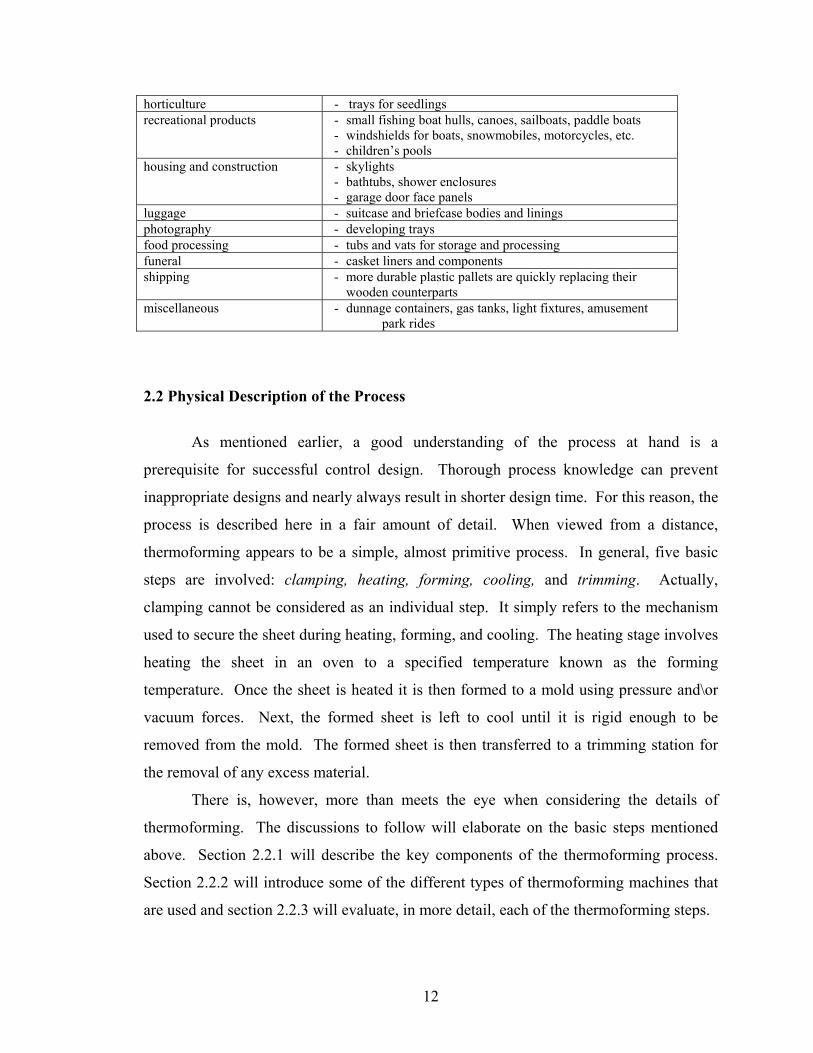
horticulture - trays for seedlings recreational products - small fishing boat hulls, canoes, sailboats, paddle boats
- windshields for boats, snowmobiles, motorcycles, etc. - children’s pools
housing and construction - skylights - bathtubs, shower enclosures - garage door face panels
luggage - suitcase and briefcase bodies and linings photography - developing trays food processing - tubs and vats for storage and processing funeral - casket liners and components shipping - more durable plastic pallets are quickly replacing their
wooden counterparts miscellaneous - dunnage containers, gas tanks, light fixtures, amusement
park rides
2.2 Physical Description of the Process
As mentioned earlier, a good understanding of the process at hand is a
prerequisite for successful control design. Thorough process knowledge can prevent
inappropriate designs and nearly always result in shorter design time. For this reason, the
process is described here in a fair amount of detail. When viewed from a distance,
thermoforming appears to be a simple, almost primitive process. In general, five basic
steps are involved: clamping, heating, forming, cooling, and trimming. Actually,
clamping cannot be considered as an individual step. It simply refers to the mechanism
used to secure the sheet during heating, forming, and cooling. The heating stage involves
heating the sheet in an oven to a specified temperature known as the forming
temperature. Once the sheet is heated it is then formed to a mold using pressure and\or
vacuum forces. Next, the formed sheet is left to cool until it is rigid enough to be
removed from the mold. The formed sheet is then transferred to a trimming station for
the removal of any excess material.
There is, however, more than meets the eye when considering the details of
thermoforming. The discussions to follow will elaborate on the basic steps mentioned
above. Section 2.2.1 will describe the key components of the thermoforming process.
Section 2.2.2 will introduce some of the different types of thermoforming machines that
are used and section 2.2.3 will evaluate, in more detail, each of the thermoforming steps.
13
2.2.1 Components of Thermoforming
2.2.1.1 Sheets
The thermoplastic sheet is the most important component of the entire
thermoforming process. Its role is obvious. Upon forming, the sheet is transformed into
a useful article. The molecular composition of the sheet is a determining factor in both
the processing steps and final part quality. The name, “poly-mer” indicates that sheets
are composed of many (poly) interconnected units (mer) that form carbon-hydrogen
chain structures. The length and entanglement of these chains are key factors in the
thermoforming process. Long molecular chains will have large molecular weights, and
will therefore be stronger than polymers consisting of short molecular chains, which tend
to be more brittle. In fact, one of the most basic requirements of a formable
thermoplastic sheet is that it has a high melt strength (high molecular weight), which
means that upon softening, the material is capable of supporting its own weight. In
contrast, a material with a low melt strength (low molecular weight) will soften once the
glass transition temperature is reached and easily tear away from the clamping
mechanism as the sheet succumbs to gravity.
Thermoplastic materials can be either amorphous or partially crystalline. As with
molecular weight, the degree of crystalinity is a determining factor in the thermoforming
process. Generally, a material with a higher degree of crystallinity requires a higher
forming temperature than for an amorphous thermoplastic. On the other hand,
amorphous materials are usually crystal clear which can be an important issue depending
on the heating mechanism used. The last point will become clear later on in the
discussion.
Now that we know material properties are key factors in the thermoforming
process, it is useful to briefly discuss how the various sheet manufacturing methods can
affect some material properties. Thermoplastic resins, which are primarily derived from
crude oil, coal, and natural gas, are manufactured into pellet form. Thermoplastic sheets
are then manufactured from these small pellets. There are a number of different ways in
which sheets can be produced, however, three methods dominate.
14
1. Calendaring
Calendaring is a similar method to paper making. First, the small pellets are fed
into large feed rolls. The pellets are then melted and forced into sheet form as the
material passes through subsequent sets of rollers. This method of sheet manufacturing
generates no molecular orientation in the sheet, which results in slightly weaker sheets
that will be subject to increase sagging during the heating process. Calendaring is also
subject to the problem of pinholes, which are tiny voids in the sheet caused by an
insufficient supply of feed pellets. Pinholes allow air to escape through he sheet, which
complicates the forming and can sometimes render a sheet useless. Fortunately, newer
manufacturing equipment has reduced the occurrence of pinholes. Nevertheless, it is still
a problem that can surface from time to time.
2. Casting
Casting involves pouring a liquid plastic into a mold and then letting the material
cool and harden to form a solid plastic sheet. For some materials casting is the only
method suitable for the production of sheet forms of the material. As with calendaring,
casting does not result in any molecular orientation. Sheets made by the casting method
are typically free of pinholes. They also have no hidden residual strains and have equal
strength in all directions. The casting method can produce tiny bubbles of trapped air
within the sheet. This can sometimes affect further sheet processing as well as the
appearance of sheets that are designed to be completely transparent.
3. Extruding
Extruding is the most popular method for manufacturing thermoplastic sheets.
The pellets enter the extruder barrel through a feed hopper. The pellets melt and the
liquid material is then squeezed through a die into sheet form. The sheet is then pressed
through a series of rollers that are spaced to give the sheet its proper thickness. Unlike
the previous two methods, extrusion results in a sheet that can contain biaxial orientations
as a result of extrusion through the die and stretching between the rollers. This orientation
results in a stronger sheet that is more resistant to sag during heating.
15
Sheet Sizes and Materials
Each of the three sheet producing methods is capable of producing a wide range
of sheet sizes. As calendaring and extrusion operations produce wound rolls of
thermoplastic materials, the sheet thickness for these operations is limited. Casting on
the other hand can produce much thicker sheets. Generally sheet thickness can range
from 0.05 mm to 15 mm and up to 60 mm for some foams. Sheet sizes for
thermoforming operations range from small sheets (< 30 cm2) to sheet sizes in the range
of 3 m x 3 m and larger. It is important to note that part sizes and thus sheet sizes are
only limited by the size of the machine, keeping in mind that the larger the part, the
greater the forming force that is required.
There are now many different types of materials that are used with
thermoforming. All materials possess their own distinctive qualities and behave
differently throughout the thermoforming process. The selection of thermoformable
materials is now so varied that the choice of part material has become one of the most
important thermoforming design steps. Some of the more common materials include:
Polystyrene (PS), Toughened Polystyrene (HIPS), Acrylonitrile-Butadiene-Styrene
(ABS), Low and High Density Polyethylene (LDPE and HDPE), Polypropylene (PP), and
Polyvinylchloride (PVC). A more detailed list of thermoforming materials including
material properties can be found in [2].
Material Properties and How They Relate to Thermoforming
As previously mentioned, material properties can have a direct effect on part
formability as well as final part quality. Some of the more important properties and their
effects will be identified in this section.
1. Moisture Absorption
Some thermoplastic materials are hydroscopic (ie. they have the ability to absorb
moisture). Moisture is predominantly retained on the sheet surface, and when a damp
material is heated, small bubbles will form on the sheet surface. At the very least,
retained moisture will affect heating times. In more severe cases moisture can damage
the appearance of the part or even affect the structural properties of the part. In these
16
cases the part is often rejected. It is easy to see why some thermoforming operations
include sheet drying as an important pre-processing step.
2. Frictional Behavior
The frictional properties of a sheet are normally only a concern when using plug-
assist techniques to further stretch certain areas of the sheet. The frictional behavior
depends on the sheet and tool (i.e. the plug) material and surface finish. If there is
insufficient friction the tool will tend to want to push directly through the sheet, which
will result in an uneven part wall thickness distribution. Conversely, too much friction
will cause the sheet to stick to the tool upon contact, which will also result in uneven
thickness distribution. It is very tricky to obtain the proper amount of frictional forces.
Slight changes to the tooling surface as well as the tooling and sheet temperatures are
required to obtain the desired results.
3. Shrinkage
Shrinkage of polymer materials is an important issue in all polymer processing
operations. Shrinkage, and particularly warpage, is important because the integrity of the
part is directly affected (i.e. strict repeatable part dimension tolerances are desirable). In
severe cases, parts can be rejected due to shrinkage and warpage. In thermoforming,
shrinkage can affect the performance of downstream processes such as trimming
operations. Some degree of shrinkage is generally unavoidable in polymer processing
operations and it is considered in the part design.
4. Orientations
As mentioned earlier molecular orientation affects the strength of a material. The
level of orientation is determined by the material, and the way in which it was produced.
If a material is stretched in one direction the material generally becomes stronger in that
direction and weaker in the opposite direction. Material strength not only comes into
play during heating (i.e. resistance to sag), it also is important for the final formed part.
The forming process stretches the material and this causes a further degree of orientation

17
which will affect the strength of the final part. All of this must be considered in the
overall part design.
5. Static Charging
Except for electrically conductive materials, thermoplastic sheets become
electrostaticly charged during material handling and processing. As a consequence, small
particles such as plastic saw chips can become attached to the surface and subsequently
embed themselves into the surface during forming resulting in parts of lower aesthetic
quality. Care must therefore be taken to ensure a clean production environment.
Thermoformable Materials and Types of Thermoplastic Sheets
As mentioned before, one of the advantages of thermoforming is that a number of
different types of sheets can be used. Table 2.2 lists types of thermoplastic sheets that are
available.
Table 2.2: types of thermoplastic sheets used for thermoforming
Sheet Type Comments Natural - made from resins without fillers of additives
- usually crystal clear - can transmit infrared heat energy
Oriented - very sensitive to heat as loss of orientation is very close to softening temperature
- requires precise and fast heating Tinted - sheets with dye additives
- sometimes slight improvement in heat absorption Pigmented - uniform colored sheets Filed - additives added to sheet for purposes of reduced cost or an
improvements in physical characteristics Foamed - much lighter material
- when colored foams are desired only light colors are possible Textured - sheets with patterns imprinted by textured rollers laminated - multi-layered sheets usually for economic reasons co-extruded - multi-layered sheets
- usually fast and easy to manufacture printed - sheets with pre-printed text or images flocked - sheets with soft velvet like finish on one side metallic - sheets with metallic coatings can be made but these are not
popular specialty - many other kinds of specialty sheets are possible
18
2.2.1.2 Clamping Mechanisms
The clamping mechanism provides the following functions: 1) support of the
sheet during sheet heating; 2) transporting heated sheet to forming area; 3) firmly holds
sheet during forming and cooling; 4) implementation of part removal; 5) transfer from
forming to trimming stations. There are two basic types of clamping mechanisms: 1)
clamp frame, and 2) transport chain mechanisms.
The clamp frame is capable of handling a single sheet at a time. The sheet is
clamped between two matching frames. One frame is usually stationary (lower) while
the other frame (upper) is hinged to allow insertion of the sheet. The frame can be
operated manually or automatically for more sophisticated higher volume machines. One
important consideration is the grip the frame has on the sheet. It is vital that the sheet
does not slip during heating or forming. Often matching grooves and even pins are
required to hold the sheet in place.
The other type of clamping mechanism is the transport chain, which is used for
continuously fed machines (see section 2.2.2). The transport chains function as the two
parallel sides of a clamp frame and carry the sheet through the oven and then on to the
forming station. Again it is important that the sheet be properly secured with the use of
high pressure forces and sometimes pins as well.
One important consideration for both types of clamping setups is the heating of
the clamping mechanism. In operations where production rates are high, clamping
mechanisms will repeatedly enter the oven and eventually heat up over time. If this
heating is significant, sheet heating will be affected as the heat from the clamping
mechanisms will be transferred to the sheet. Also, care must be taken to ensure that the
heat build up is not excessive as the clamping mechanism may actually melt the plastic
sheet. Excessive heating can sometimes be avoided in radiation heating ovens by
applying reflective paint to the clamping components.
2.2.1.3 Heating Systems
The heating system is a key element of the thermoforming process. Regardless of
the heat source, the application of heat must be relatively precise and repeatable in order
to have predictable cycle-to-cycle results. The heating system is also a key factor when
19
examining the economics of a thermoforming operation because thermoforming is an
energy intensive process and heating of the sheet accounts for up to 80% of the energy
consumption. Two basic energy sources are available for sheet heating: gas and
electricity. Gas is much less expensive than electricity but the latter offers much better
temperature control. Although there is a wide variety of specific heating methods and
heater types available, there are only three basic heating methods applied to
thermoforming.
The first is gas fired convection ovens. These ovens are usually very large to
accommodate the heating of large, extra thick sheets. Cycle times for these larger sheets
tend to be measured in hours as opposed to seconds; therefore, it is obvious that electrical
heating is not economically feasible. The sheet itself is actually heated by hot air that is
forced over the sheet surfaces by large blowers. Although these gas fired ovens offer less
controllable heating, the size and bulk of these larger sheets does not warrant such close
temperature control.
The second method is contact heating. This setup consists of heated metal plates
that directly contact the sheet to heat it. The metal plates can be heated by either a gas
flame or by electrical strip heaters either embedded or mounted to the opposite surface of
the plate. In this type of heating it is important to ensure proper contact with the sheet.
Uneven contact can trap air between the plate and the sheet and cause uneven heating.
This method is limited to uniform heating (no zoning) of thinner thermoplastic sheets.
Because this method of heating is quite slow, the sheet is sometimes preheated with other
heating methods to increase production speed.
The final method of heating is radiant heating. Radiant heating methods are
definitely the most popular because of their controllability and efficiency. No contact is
needed in this method. The sheet surface absorbs infrared energy from the heaters, and
heat is then conducted from the sheet surfaces to the interior of the sheet. Gas fired
radiant heaters are sometimes used but electrical radiant heaters are much more common.
Electrical radiant heaters can operate over a very wide temperature range; however, the
best electrical to radiation conversion efficiency occurs when the heaters operate at
temperatures that produce infrared energy concentrated at wavelengths of between 3 to
3.5 µm. More will be said later about the infrared spectrum. Since electrical heaters are
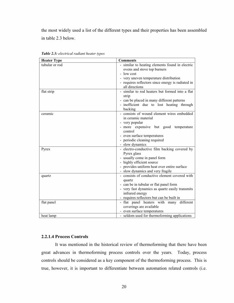
20
the most widely used a list of the different types and their properties has been assembled
in table 2.3 below.
Table 2.3: electrical radiant heater types
Heater Type Comments tubular or rod - similar to heating elements found in electric
ovens and stove top burners - low cost - very uneven temperature distribution - requires reflectors since energy is radiated in
all directions flat strip - similar to rod heaters but formed into a flat
strip - can be placed in many different patterns - inefficient due to lost heating through
backing ceramic - consists of wound element wires embedded
in ceramic material - very popular - more expensive but good temperature
control - even surface temperatures - periodic cleaning required - slow dynamics
Pyrex - electro-conductive film backing covered by Pyrex glass
- usually come in panel form - highly efficient source - provides uniform heat over entire surface - slow dynamics and very fragile
quartz - consists of conductive element covered with quartz
- can be in tubular or flat panel form - very fast dynamics as quartz easily transmits
infrared energy - requires reflectors but can be built in
flat panel - flat panel heaters with many different coverings are available
- even surface temperatures heat lamp - seldom used for thermoforming applications
2.2.1.4 Process Controls
It was mentioned in the historical review of thermoforming that there have been
great advances in thermoforming process controls over the years. Today, process
controls should be considered as a key component of the thermoforming process. This is
true, however, it is important to differentiate between automation related controls (i.e.
21
material handling, cycle timers, heater controls, etc.) and feedback control of process
parameters. The improvements have been with machine automation whereas the
application of feedback control, such as control of sheet temperature, has been virtually
nonexistent.
Feedback control of the heater settings is nearly universal on modern machines so
it is worth mentioning here. There are basically two types of temperature controllers
available. The first type uses switched, or on-off control, to regulate the heater
temperatures. In this type of control, full power is intermittently sent to the heaters. The
second type of control is slightly more sophisticated. It uses power electronic devices to
supply varying power levels to the heaters in order to maintain the setpoint. Both types
of control result in oscillations about the setpoint with the on-off control oscillations
being more prominent. Oscillations are rarely a problem, however, when heaters have a
relatively high thermal mass. This is the case with the popular ceramic heater, which is
designed to maintain a constant surface temperature without responding to small power
fluctuations. Machine automation procedures and equipment vary extensively. Because
there are so many different types of machines available a full discussion of machine
automation is beyond the scope of this work.
2.2.1.5 Molds
Occasionally molds are not required to form a sheet, as is the case with “free-
blow” forming methods used to make skylight windows for homes. The vast majority of
forming operations do require molds for shaping the plastic sheet. The primary purpose
of the mold then is to transform its shape to the heated, flat plastic sheet. The sheet is
either forced into or drawn over a mold. Three different types of molds exist. All have
different qualities and will leave distinctive characteristics implanted into the formed
part. All three molds can be found in single or multi-up forms. A single mold uses a
single sheet to form one individual part. A multi-up mold forms an array of multiple
parts from the same plastic sheet. A number of considerations are important for all mold
types. For example, part shrinkage considerations and mold venting are important design
issues. Mold material is also an issue that requires some thought. Thermoforming molds
are usually made from aluminum. Epoxy materials are sometimes used, and even wood
22
can be used to construct a mold. The mold material is generally dictated by the intended
use and life expectancy of the mold.
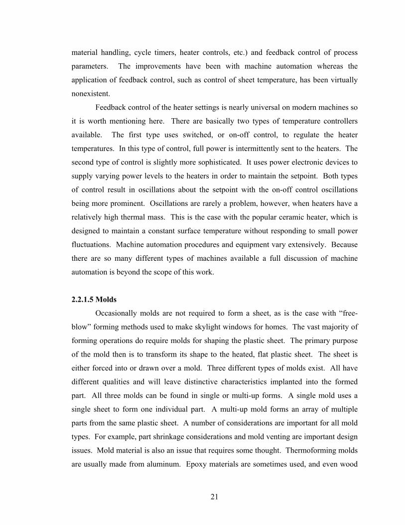
Female molds
For the female mold shown in figure 2.2a the heated sheet is drawn into the mold
cavity by either pressure or vacuum forces, or a combination of both. A female mold
results in less characteristic evidence of the mold on the part, which means that female
molds are often not used where intricate details are required on the part surface. Since
the part will shrink during cooling the part will actually begin to pull away from the mold
walls which results in easy part removal. As can be seen in figure 2.2b, most of the
stretching occurs at the bottom of the sheet whereas the flange areas remain close to the
original part thickness. This suggests that even material distribution before forming does
not result in a part with even wall thickness.
Figure 2.2a: basic female mold Figure 2.2b: material distribution for
female molded part
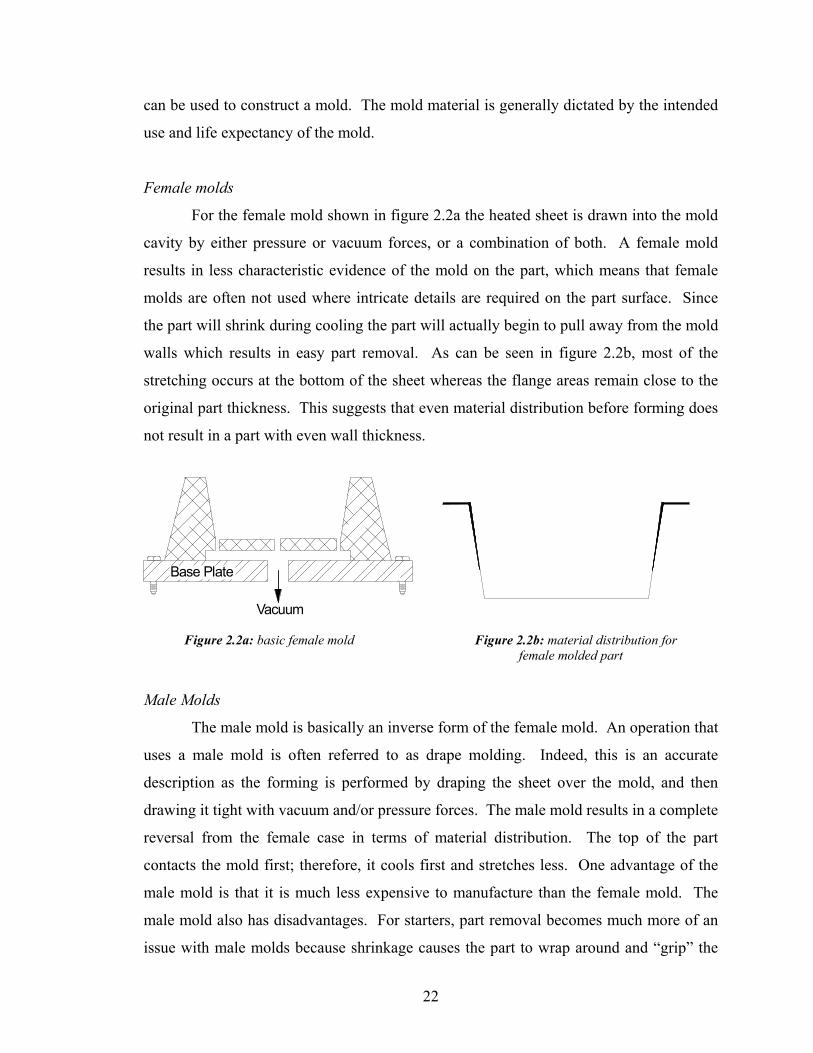
Male Molds
The male mold is basically an inverse form of the female mold. An operation that
uses a male mold is often referred to as drape molding. Indeed, this is an accurate
description as the forming is performed by draping the sheet over the mold, and then
drawing it tight with vacuum and/or pressure forces. The male mold results in a complete
reversal from the female case in terms of material distribution. The top of the part
contacts the mold first; therefore, it cools first and stretches less. One advantage of the
male mold is that it is much less expensive to manufacture than the female mold. The
male mold also has disadvantages. For starters, part removal becomes much more of an
issue with male molds because shrinkage causes the part to wrap around and “grip” the
Vacuum
Base Plate
23
mold. Pressurized air is often used for part removal. Another disadvantage is that it is
much more difficult to implement multi-up molds. Spacing is more critical than with
female molds since the majority of the stretching and material thinning will take place
between the molds and not over the mold area. Figure 2.3a shows a basic male mold.
Figure 2.3a: basic male mold Figure 2.3b: material distribution for male molded part
Matched Molds
In its purest form matched molding sees a sheet being mechanically forced into a
female mold by a matching male mold. Variations also exist where air pressure and/or
vacuum forces are also used. Mold alignment is a very important issue in matched
molding. Small misalignment will result in rejected parts. On advantage of matched
molds is that it is possible to get different surface features on opposite sides of the part.
Mold Temperature
The second, and equally important, function of the mold is to absorb heat from the
sheet. For high volume productions a mold will heat up to a point where its temperature
will match that of the sheet; therefore, some form of auxiliary cooling is generally
required. Thermoforming molds can be cooled simply by airflow over their surfaces or
internal liquid cooling channels. The mold must not be cooled so much as to cause poor
forming detail or possibly uneven stretching of the sheet. Some operations do not require
mold cooling as enough heat is dissipated to the ambient environment. Some low volume
productions actually require auxiliary mold heating because some thermoplastic materials
require elevated mold temperatures for proper forming. Mold heating can be achieved
via electrical heating or circulation of heated fluids (usually water or oil) through the
Vacuum
Base Plate
24
interior of the mold. Proper mold temperatures are critical for the production of a
successful part. Sheet manufacturers usually give an ideal mold temperature range but
there is always a certain level of fine-tuning involved.
2.2.2 Thermoforming Machines
Thermoforming machines come in a wide variety of shapes and sizes. Machines
are often specially designed for the purpose of making a particular part. Some machines
can be considered to be more general purpose but these machines often lack the high-
speed production capabilities of their specialized cousins. Much could be said about the
many thermoforming machine variants but is does not really add to this discussion. Only
the basics will be discussed in the remainder of this section.
Thermoforming machines come in two basic types: sheet fed and roll fed. Both
types can have varying levels of sophistication and automation. A wide range of sizes are
also available for both types. The size of a machine is generally measured by the mold
size that can be accommodated and the amount of forming force that is available.
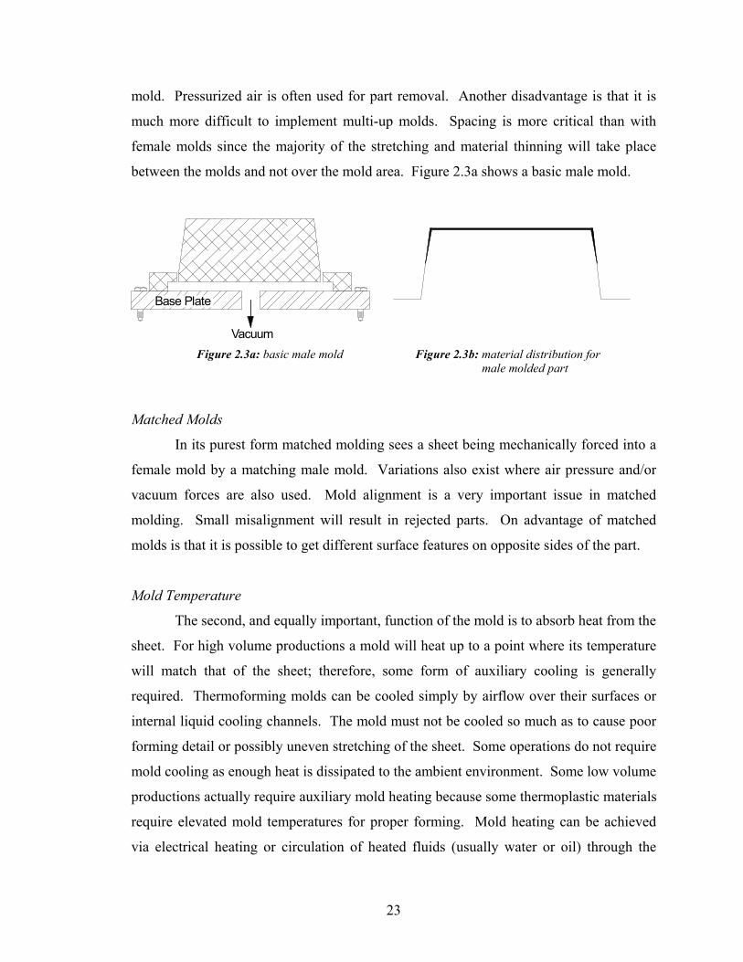
2.2.2.1 Sheet Fed
The sheet fed machine can generally accommodate only one sheet at a time
except for twin sheet thermoforming machines which process two sheets simultaneously.
The simplest sheet fed machine is the stationary machine, where the sheet is heated and
formed in the same location. Shuttle thermoforming machines such as the one shown in
figure 2.4 are more common. The basic feature of the shuttle machine is that the clamped
sheet is shuttled in and out of the sheet heating area. A number of variations can be
found but the basic operating principle remains the same. One variation that is worth
mentioning is the rotary shuttle thermoforming machine. For this machine the sheet is
still shuttled from station to station but the stations are arranged in a compact circular
arrangement, which improves speed and efficiency.
25
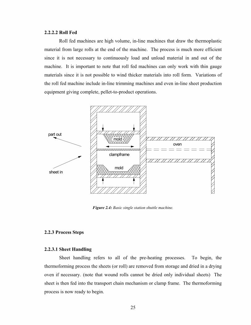
2.2.2.2 Roll Fed
Roll fed machines are high volume, in-line machines that draw the thermoplastic
material from large rolls at the end of the machine. The process is much more efficient
since it is not necessary to continuously load and unload material in and out of the
machine. It is important to note that roll fed machines can only work with thin gauge
materials since it is not possible to wind thicker materials into roll form. Variations of
the roll fed machine include in-line trimming machines and even in-line sheet production
equipment giving complete, pellet-to-product operations.
mold
mold
oven
clampframe
sheet in
part out
Figure 2.4: Basic single station shuttle machine.
2.2.3 Process Steps
2.2.3.1 Sheet Handling
Sheet handling refers to all of the pre-heating processes. To begin, the
thermoforming process the sheets (or roll) are removed from storage and dried in a drying
oven if necessary. (note that wound rolls cannot be dried only individual sheets) The
sheet is then fed into the transport chain mechanism or clamp frame. The thermoforming
process is now ready to begin.
26
2.2.3.2 Sheet Heating
Sheet heating, or reheat, is probably the single most important step because the
results of sheet reheat can affect all subsequent processing steps. The focus of this work
is almost exclusively on the reheat stage. One of the main motivating factors for
developing an in-cycle control strategy is the fact that the reheat stage has been
essentially untouched by advances in process control technology. Also, the reheat stage
is the only step in which it is even possible to make any significant improvements
through the application of model based control techniques.
The two controlling factors for the sheet reheat stage are heater temperature
settings and heating time. The goal of sheet reheat is to bring the sheet centerline
temperature up to the minimum forming temperature as quickly as possible. For
radiation heating, the sheet surface temperature will increase very rapidly, and it will
continue to rise so long as the sheet remains in the oven. It is very important to set the
heater temperatures such that the sheet surface temperature does not rise above the
maximum allowable temperature. If the sheet surface temperature does become too high
there is a strong possibility of material degradation and even scorching of the sheet
surface, which will result in a rejected part. It is also important to limit the heating rate
for some materials. A heating rate that is too fast can cause loss of molecular orientation,
surface degradation, and for foamed materials, foam breakdown due to poor material
expansion. The maximum allowable heating rate will be dictated by the application of
the part and the type of thermoplastic sheet.
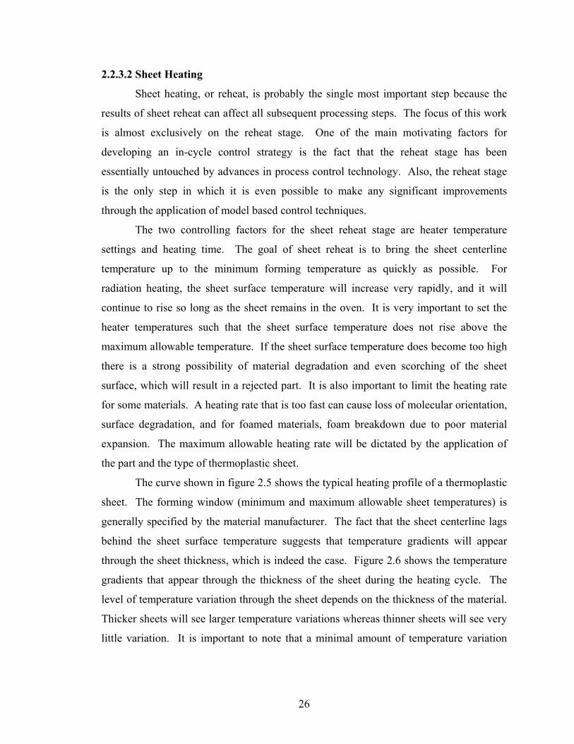
The curve shown in figure 2.5 shows the typical heating profile of a thermoplastic
sheet. The forming window (minimum and maximum allowable sheet temperatures) is
generally specified by the material manufacturer. The fact that the sheet centerline lags
behind the sheet surface temperature suggests that temperature gradients will appear
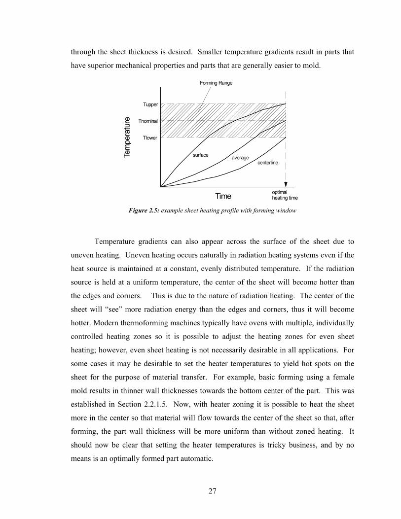
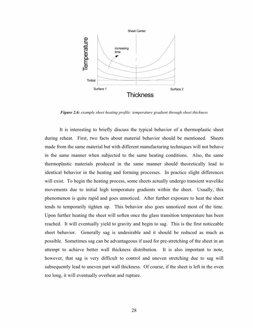
through the sheet thickness, which is indeed the case. Figure 2.6 shows the temperature
gradients that appear through the thickness of the sheet during the heating cycle. The
level of temperature variation through the sheet depends on the thickness of the material.
Thicker sheets will see larger temperature variations whereas thinner sheets will see very
little variation. It is important to note that a minimal amount of temperature variation
27
through the sheet thickness is desired. Smaller temperature gradients result in parts that
have superior mechanical properties and parts that are generally easier to mold.
Time
Tem
pera
ture
optimal heating time
Forming Range
Tupper
Tnominal
Tlower
surface averagecenterline
Figure 2.5: example sheet heating profile with forming window
Temperature gradients can also appear across the surface of the sheet due to
uneven heating. Uneven heating occurs naturally in radiation heating systems even if the
heat source is maintained at a constant, evenly distributed temperature. If the radiation
source is held at a uniform temperature, the center of the sheet will become hotter than
the edges and corners. This is due to the nature of radiation heating. The center of the
sheet will “see” more radiation energy than the edges and corners, thus it will become
hotter. Modern thermoforming machines typically have ovens with multiple, individually
controlled heating zones so it is possible to adjust the heating zones for even sheet
heating; however, even sheet heating is not necessarily desirable in all applications. For
some cases it may be desirable to set the heater temperatures to yield hot spots on the
sheet for the purpose of material transfer. For example, basic forming using a female
mold results in thinner wall thicknesses towards the bottom center of the part. This was
established in Section 2.2.1.5. Now, with heater zoning it is possible to heat the sheet
more in the center so that material will flow towards the center of the sheet so that, after
forming, the part wall thickness will be more uniform than without zoned heating. It
should now be clear that setting the heater temperatures is tricky business, and by no
means is an optimally formed part automatic.
28
Tinitial
Surface 1 Surface 2
Sheet Center
ThicknessTe
mpe
ratu
re
increasing time
Figure 2.6: example sheet heating profile: temperature gradient through sheet thickness
It is interesting to briefly discuss the typical behavior of a thermoplastic sheet
during reheat. First, two facts about material behavior should be mentioned. Sheets
made from the same material but with different manufacturing techniques will not behave
in the same manner when subjected to the same heating conditions. Also, the same
thermoplastic materials produced in the same manner should theoretically lead to
identical behavior in the heating and forming processes. In practice slight differences
will exist. To begin the heating process, some sheets actually undergo transient wavelike
movements due to initial high temperature gradients within the sheet. Usually, this
phenomenon is quite rapid and goes unnoticed. After further exposure to heat the sheet
tends to temporarily tighten up. This behavior also goes unnoticed most of the time.
Upon further heating the sheet will soften once the glass transition temperature has been
reached. It will eventually yield to gravity and begin to sag. This is the first noticeable
sheet behavior. Generally sag is undesirable and it should be reduced as much as
possible. Sometimes sag can be advantageous if used for pre-stretching of the sheet in an
attempt to achieve better wall thickness distribution. It is also important to note,
however, that sag is very difficult to control and uneven stretching due to sag will
subsequently lead to uneven part wall thickness. Of course, if the sheet is left in the oven
too long, it will eventually overheat and rupture.
29
2.2.3.3 Forming
Once the sheet is heated it is ready to be formed. Forming is necessary in order to
transfer the shape of the mold to the sheet. As mentioned earlier, nearly all
thermoforming operations use either male, female, or matched molds. Forming can be
classified based on whether pressure or vacuum forces are used. Vacuum forming is
more widely used but the application of pressure forming forces is growing since it is
possible to obtain higher part definition with the larger pressure forces than with the
smaller vacuum forces. Many different forming methods exist. The most popular are
explained well in [3]. One common goal that all of these forming methods have is even
material distribution, which can be generalized as the ultimate goal of the thermoformer.
2.2.3.4 Cooling
The next step in the thermoforming process is part cooling. The material must
cool until it is completely rigid before it can be ejected from the mold. The cooling is
performed by the mold itself and sometimes auxiliary fans are used to blow ambient air
over the part to cool it more quickly. Sometimes, misting equipment is also used in
conjunction with fans to cool the part even faster. As with the heating rate, the cooling
rate must also be considered since the cooling rate affects material crystallization, which
can be a determining factor in the mechanical properties of the part. Factors that affect
the cooling time include: 1) sheet material; 2) sheet thickness; 3) forming temperature;
4) mold material; 5) mold temperature; 6) contact intensity between the mold and sheet.
2.2.3.5 Trimming
Once the part is formed and cooled it is removed from the mold and transferred to
a trimming station. For a single part made from a single sheet, the sheet material that was
used for clamping usually needs to be removed. This material is often referred to as flash
material in the polymer processing industry. For multiple parts made from a single sheet
of material the flash material includes the clamping material as well as the material
between the molds. Trimming can be performed manually using hand held knives or
power tools but this technique is usually reserved for operations that produce a small
30
number of parts. Usually automated equipment such as punch and die sets, or even
robotic cutting systems are used.
This section provided a description of the thermoforming process in a level of
detail that will allow the reader to comfortably move through the remainder of this thesis
with sufficient background information. This section was, however, only an introduction
to thermoforming. Many good works are available in the literature, including [1], if a
deeper knowledge of the subject is required.
2.3 IMI Equipment Description
An industrial scale thermoforming machine located at the IMI facility was used
for all experimentation and testing that was required for completion of this project. The
original machine is actually quite old, but it has been retrofitted over the years. It can
now be considered a suitable “research” or “experimental” machine.
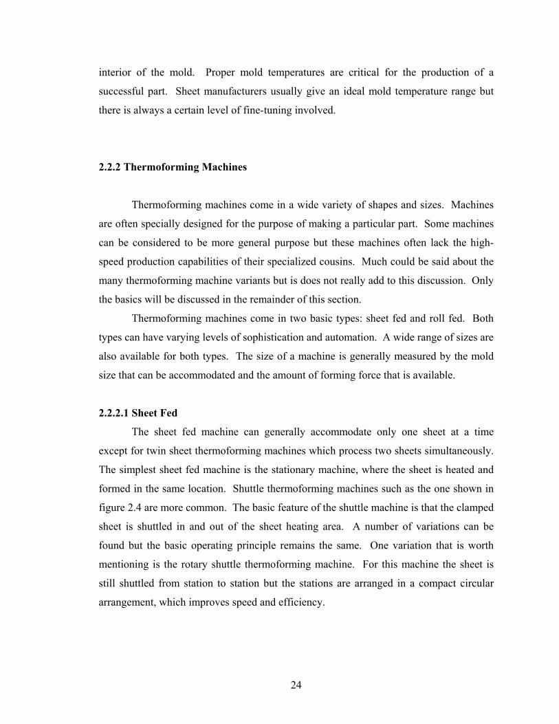
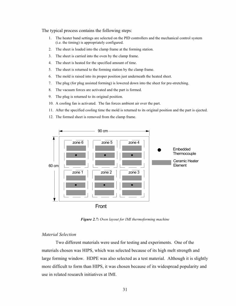
The IMI machine is a simple, single oven, single forming station shuttle
thermoforming machine capable of sheet sizes up to approximately 60 x 90 cm. The
sheet heating is performed by an upper and lower radiation heating oven, each with six
individually controlled heater zones (figure 2.7) for a total of twelve heater zones. The
center heater in each zone has an embedded thermocouple for temperature feedback
measurements. It is common practice not to have temperature feedback for all individual
heater elements since it is not economically feasible to control each individual element.
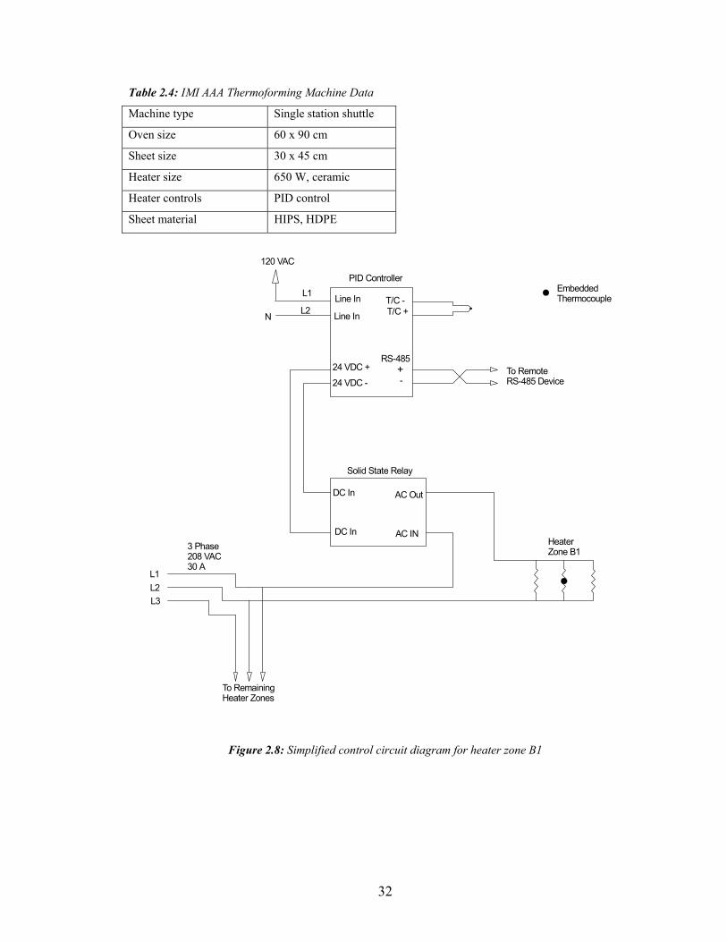
The temperature control (figure 2.8) is performed via PID controllers that are tuned using
their convenient auto-tune feature.
The timing of the processing steps are controlled by a rather old mechanical
thumbwheel system where the process steps are selected by inserting pegs into
appropriate slots in the “wheel”. The timing for each step is adjusted using a series of
thumbwheel switches.
31
The typical process contains the following steps: 1. The heater band settings are selected on the PID controllers and the mechanical control system
(i.e. the timing) is appropriately configured.
2. The sheet is loaded into the clamp frame at the forming station.
3. The sheet is carried into the oven by the clamp frame.
4. The sheet is heated for the specified amount of time.
5. The sheet is returned to the forming station by the clamp frame.
6. The mold is raised into its proper position just underneath the heated sheet.
7. The plug (for plug assisted forming) is lowered down into the sheet for pre-stretching.
8. The vacuum forces are activated and the part is formed.
9. The plug is returned to its original position.
10. A cooling fan is activated. The fan forces ambient air over the part.
11. After the specified cooling time the mold is returned to its original position and the part is ejected.
12. The formed sheet is removed from the clamp frame.
Front
90 cm
60 cm
EmbeddedThermocouple
Ceramic HeaterElement
zone 6
zone 1 zone 2 zone 3
zone 5 zone 4
Figure 2.7: Oven layout for IMI thermoforming machine
Material Selection
Two different materials were used for testing and experiments. One of the
materials chosen was HIPS, which was selected because of its high melt strength and
large forming window. HDPE was also selected as a test material. Although it is slightly
more difficult to form than HIPS, it was chosen because of its widespread popularity and
use in related research initiatives at IMI.
32
Table 2.4: IMI AAA Thermoforming Machine Data Machine type Single station shuttle
Oven size 60 x 90 cm
Sheet size 30 x 45 cm
Heater size 650 W, ceramic
Heater controls PID control
Sheet material HIPS, HDPE
Line In
Line In
120 VAC
N
T/C -T/C +
RS-48524 VDC +24 VDC -
+
-
PID Controller
Solid State Relay
DC In
DC In
AC Out
AC INHeaterZone B1
Embedded ThermocoupleL1
L2
L1
L3L2
3 Phase208 VAC30 A
To Remote RS-485 Device
To Remaining Heater Zones
Figure 2.8: Simplified control circuit diagram for heater zone B1
33
3. Process Modeling
3.1 Introduction
Developing deterministic process models is usually the first step in any model
based control design project. This project was no different. A full order, finite element
simulation model of the thermoforming process had been previously developed by
research associates at IMI; however, this large, very complex model is not suitable for the
design of implementable, low order controllers. Development of a low order, process
model, is therefore required.
Generally there are two basic methodologies that are available for process
modeling. The first is the direct, first principles approach which utilizes in depth
knowledge of the system and various laws of physics (i.e. conservation of mass, energy,
etc.) to obtain mathematical equations which describe the system’s behavior. The second
approach is commonly referred to as the “black box” modeling approach. This approach
uses system identification techniques to obtain mathematical models from experimental
input-output data.
The first principles approach has some distinct advantages. To start, the
mathematical equations that are derived have physical meaning. Each of the terms in the
equations relates to a specific physical phenomenon which yields greater insight into
system behavior. As a result, it is possible to tune the parameters in the model so that the
model better represents the actual physical system. This also leads to a more flexible
design since it is possible to simplify or expand upon the model as required. Another
advantage is the fact this approach generally does not require as many model validation
and identification experiments. Finally, the first principles approach usually results in
better extrapolation performance. This means that the model will often describe, quite
well, the behavior of the system in operating ranges that are outside of the range in which
the identification and validation experiments were performed.
Of course there are also drawbacks of the first principles approach. One
important drawback, which is of major concern, is the fact that a lot of time and effort is
usually required to develop a suitable model. The model parameters can sometimes be
34
difficult to obtain, particularly when there are many uncertain parameters within the
model. This will also increase the design time. Inaccurate models are also a major
disadvantage. Modeling errors can occur when unmodeled, higher order dynamics are
left out, or when very complex physical phenomena are described by over simplified
mathematical relationships.
Like the first principles approach, the black box approach also has its own distinct
advantages and disadvantages. One advantage is that a black box model, depending on
its structure, can often better describe the behavior of the system within a certain
operating range even though the modeling equations hold no physical meaning. Another
advantage is the fact that this approach is very versatile and can be applied to a wide
range of systems. This accounts for the method’s popularity. One final advantage is the
fact that an in depth understanding of the system dynamics is not necessarily required.
As a result, the black box approach is often a practical, less labour intensive modeling
strategy.
One of the disadvantages of black box modeling is the fact that “plant friendly”
inputs are not always possible. This means that some systems may not be suitable for the
application of system identification techniques that require relatively large input
perturbations, which can subsequently bring the system out of its normal operating range
and cause a defective product or even damaged equipment. Sometimes small signal
PRBS (Pseudo Random Binary Signal) analysis is used to extract process models from
processes that are sensitive to large perturbations. Unfortunately, this technique is not
directly applicable to thermoforming due to the slow response of the heating elements.
Also, if the process is time-varying, most black box models will not be capable of
capturing the time-varying dynamics of the process. Finally, the black box approach can
sometimes require many identification experiments, which can be time consuming and
costly depending on the process. Table 3.1 summarizes the key attributes of the first
principles and black box modeling methodologies. One must ultimately choose the
appropriate modeling approach for the process at hand upon considering all of the
advantages and disadvantages of each modeling approach.
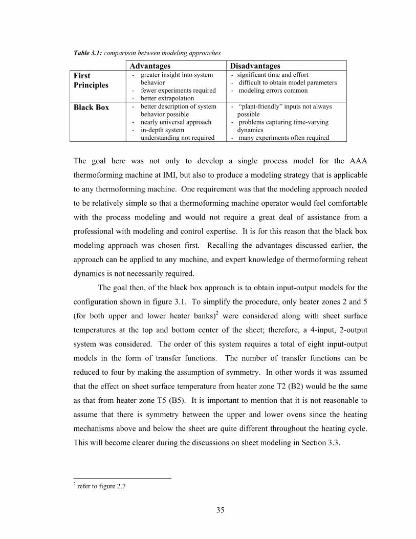
35
Table 3.1: comparison between modeling approaches
Advantages Disadvantages First Principles
- greater insight into system behavior
- fewer experiments required - better extrapolation
- significant time and effort - difficult to obtain model parameters - modeling errors common
Black Box - better description of system behavior possible
- nearly universal approach - in-depth system
understanding not required
- “plant-friendly” inputs not always possible
- problems capturing time-varying dynamics
- many experiments often required
The goal here was not only to develop a single process model for the AAA
thermoforming machine at IMI, but also to produce a modeling strategy that is applicable
to any thermoforming machine. One requirement was that the modeling approach needed
to be relatively simple so that a thermoforming machine operator would feel comfortable
with the process modeling and would not require a great deal of assistance from a
professional with modeling and control expertise. It is for this reason that the black box
modeling approach was chosen first. Recalling the advantages discussed earlier, the
approach can be applied to any machine, and expert knowledge of thermoforming reheat
dynamics is not necessarily required.
The goal then, of the black box approach is to obtain input-output models for the
configuration shown in figure 3.1. To simplify the procedure, only heater zones 2 and 5
(for both upper and lower heater banks)2 were considered along with sheet surface
temperatures at the top and bottom center of the sheet; therefore, a 4-input, 2-output
system was considered. The order of this system requires a total of eight input-output
models in the form of transfer functions. The number of transfer functions can be
reduced to four by making the assumption of symmetry. In other words it was assumed
that the effect on sheet surface temperature from heater zone T2 (B2) would be the same
as that from heater zone T5 (B5). It is important to mention that it is not reasonable to
assume that there is symmetry between the upper and lower ovens since the heating
mechanisms above and below the sheet are quite different throughout the heating cycle.
This will become clearer during the discussions on sheet modeling in Section 3.3.
2 refer to figure 2.7
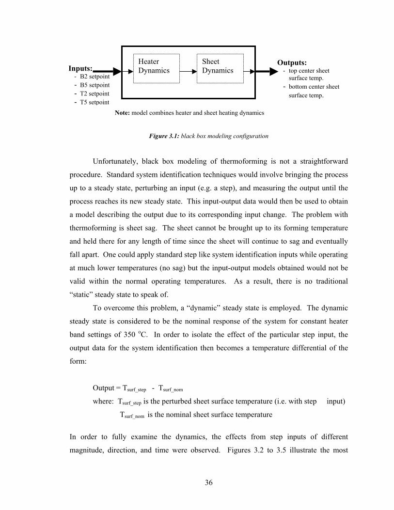
36
Figure 3.1: black box modeling configuration
Unfortunately, black box modeling of thermoforming is not a straightforward
procedure. Standard system identification techniques would involve bringing the process
up to a steady state, perturbing an input (e.g. a step), and measuring the output until the
process reaches its new steady state. This input-output data would then be used to obtain
a model describing the output due to its corresponding input change. The problem with
thermoforming is sheet sag. The sheet cannot be brought up to its forming temperature
and held there for any length of time since the sheet will continue to sag and eventually
fall apart. One could apply standard step like system identification inputs while operating
at much lower temperatures (no sag) but the input-output models obtained would not be
valid within the normal operating temperatures. As a result, there is no traditional
“static” steady state to speak of.
To overcome this problem, a “dynamic” steady state is employed. The dynamic
steady state is considered to be the nominal response of the system for constant heater
band settings of 350 oC. In order to isolate the effect of the particular step input, the
output data for the system identification then becomes a temperature differential of the
form:
Output = Tsurf_step - Tsurf_nom
where: Tsurf_step is the perturbed sheet surface temperature (i.e. with step input)
Tsurf_nom is the nominal sheet surface temperature
In order to fully examine the dynamics, the effects from step inputs of different
magnitude, direction, and time were observed. Figures 3.2 to 3.5 illustrate the most
Heater Dynamics
Sheet Dynamics
Outputs: - top center sheet
surface temp. - bottom center sheet
surface temp.
Inputs: - B2 setpoint - B5 setpoint - T2 setpoint - T5 setpoint
Note: model combines heater and sheet heating dynamics
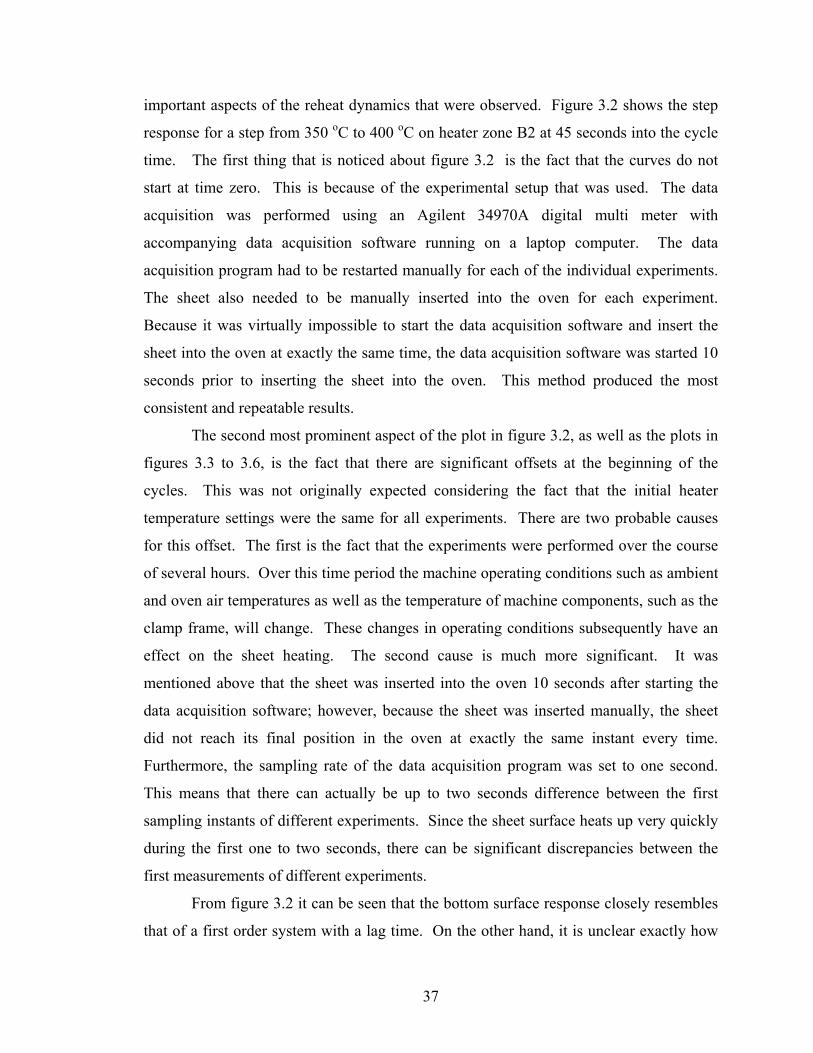
37
important aspects of the reheat dynamics that were observed. Figure 3.2 shows the step
response for a step from 350 oC to 400 oC on heater zone B2 at 45 seconds into the cycle
time. The first thing that is noticed about figure 3.2 is the fact that the curves do not
start at time zero. This is because of the experimental setup that was used. The data
acquisition was performed using an Agilent 34970A digital multi meter with
accompanying data acquisition software running on a laptop computer. The data
acquisition program had to be restarted manually for each of the individual experiments.
The sheet also needed to be manually inserted into the oven for each experiment.
Because it was virtually impossible to start the data acquisition software and insert the
sheet into the oven at exactly the same time, the data acquisition software was started 10
seconds prior to inserting the sheet into the oven. This method produced the most
consistent and repeatable results.
The second most prominent aspect of the plot in figure 3.2, as well as the plots in
figures 3.3 to 3.6, is the fact that there are significant offsets at the beginning of the
cycles. This was not originally expected considering the fact that the initial heater
temperature settings were the same for all experiments. There are two probable causes
for this offset. The first is the fact that the experiments were performed over the course
of several hours. Over this time period the machine operating conditions such as ambient
and oven air temperatures as well as the temperature of machine components, such as the
clamp frame, will change. These changes in operating conditions subsequently have an
effect on the sheet heating. The second cause is much more significant. It was
mentioned above that the sheet was inserted into the oven 10 seconds after starting the
data acquisition software; however, because the sheet was inserted manually, the sheet
did not reach its final position in the oven at exactly the same instant every time.
Furthermore, the sampling rate of the data acquisition program was set to one second.
This means that there can actually be up to two seconds difference between the first
sampling instants of different experiments. Since the sheet surface heats up very quickly
during the first one to two seconds, there can be significant discrepancies between the
first measurements of different experiments.
From figure 3.2 it can be seen that the bottom surface response closely resembles
that of a first order system with a lag time. On the other hand, it is unclear exactly how
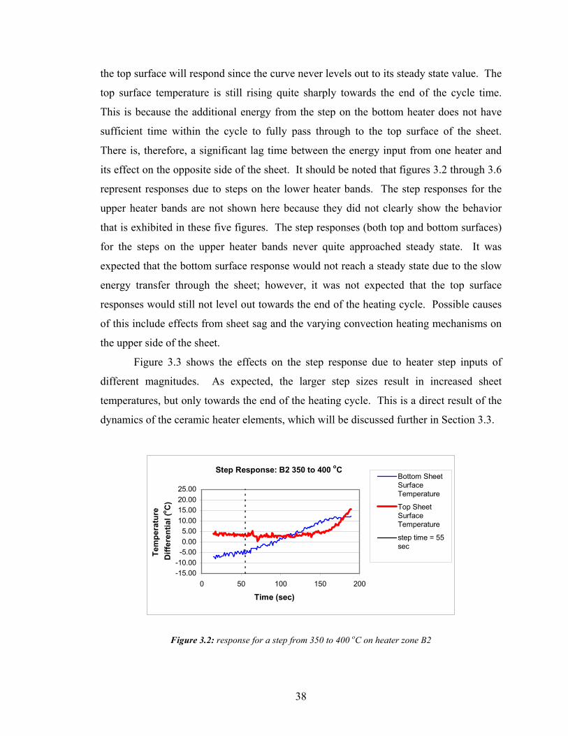
38
the top surface will respond since the curve never levels out to its steady state value. The
top surface temperature is still rising quite sharply towards the end of the cycle time.
This is because the additional energy from the step on the bottom heater does not have
sufficient time within the cycle to fully pass through to the top surface of the sheet.
There is, therefore, a significant lag time between the energy input from one heater and
its effect on the opposite side of the sheet. It should be noted that figures 3.2 through 3.6
represent responses due to steps on the lower heater bands. The step responses for the
upper heater bands are not shown here because they did not clearly show the behavior
that is exhibited in these five figures. The step responses (both top and bottom surfaces)
for the steps on the upper heater bands never quite approached steady state. It was
expected that the bottom surface response would not reach a steady state due to the slow
energy transfer through the sheet; however, it was not expected that the top surface
responses would still not level out towards the end of the heating cycle. Possible causes
of this include effects from sheet sag and the varying convection heating mechanisms on
the upper side of the sheet.
Figure 3.3 shows the effects on the step response due to heater step inputs of
different magnitudes. As expected, the larger step sizes result in increased sheet
temperatures, but only towards the end of the heating cycle. This is a direct result of the
dynamics of the ceramic heater elements, which will be discussed further in Section 3.3.
Step Response: B2 350 to 400 oC
-15.00-10.00-5.000.005.00
10.0015.0020.0025.00
0 50 100 150 200
Time (sec)
Tem
pera
ture
Diff
eren
tial (
o C)
Bottom SheetSurfaceTemperature
Top SheetSurfaceTemperature
step time = 55sec
Figure 3.2: response for a step from 350 to 400 oC on heater zone B2
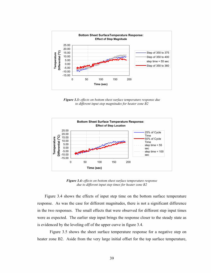
39
Bottom Sheet SurfaceTemperature Response: Effect of Step Magnitude
-15.00-10.00-5.000.005.00
10.0015.0020.0025.00
0 50 100 150 200
Time (sec)
Tem
pera
ture
Diff
eren
tial (
o C)
Step of 350 to 375Step of 350 to 400step time = 55 secStep of 350 to 360
Figure 3.3: effects on bottom sheet surface temperature response due to different input step magnitudes for heater zone B2
Bottom Sheet Surface Temperature Response: Effect of Step Location
-15.00-10.00-5.000.005.00
10.0015.0020.0025.00
0 50 100 150 200
Time (sec)
Tem
pera
ture
D
iffer
entia
l (o C
)
25% of CycleTime50% of CycleTimestep time = 55secstep time = 100sec
Figure 3.4: effects on bottom sheet surface temperature response due to different input step times for heater zone B2
Figure 3.4 shows the effects of input step time on the bottom surface temperature
response. As was the case for different magnitudes, there is not a significant difference
in the two responses. The small effects that were observed for different step input times
were as expected. The earlier step input brings the response closer to the steady state as
is evidenced by the leveling off of the upper curve in figure 3.4.
Figure 3.5 shows the sheet surface temperature response for a negative step on
heater zone B2. Aside from the very large initial offset for the top surface temperature,
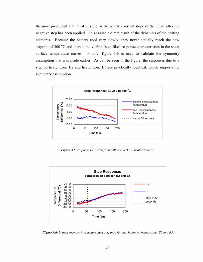
40
the most prominent feature of this plot is the nearly constant slope of the curve after the
negative step has been applied. This is also a direct result of the dynamics of the heating
elements. Because the heaters cool very slowly, they never actually reach the new
setpoint of 300 oC and there is no visible “step like” response characteristics in the sheet
surface temperature curves. Finally, figure 3.6 is used to validate the symmetry
assumption that was made earlier. As can be seen in the figure, the responses due to a
step on heater zone B2 and heater zone B5 are practically identical, which supports the
symmetry assumption.
Step Response: B2 350 to 300 oC
-15.00
-5.00
5.00
15.00
25.00
0 50 100 150 200
Time (sec)
Tem
pera
ture
D
iffer
entia
l (o C
) Bottom Sheet SurfaceTemperature
Top Sheet SurfacaeTemperature
step at 55 seconds
Figure 3.5: response for a step from 350 to 400 oC on heater zone B2
Step Response:comparisson between B2 and B5
-15.00-10.00-5.000.005.00
10.0015.0020.0025.00
0 50 100 150 200
Time (sec)
Tem
pera
ture
D
iffer
entia
l (o C
) B2
B5
step at 55seconds
Figure 3.6: bottom sheet surface temperature response for step inputs on heater zones B2 and B5
41
System Identification
The first black box system identification attempt was not successful. Matlab’s
system identification toolbox was used and numerous model structures were tried. A
model structure and order could not be found such that the resulting model had good
prediction capabilities and stability properties. We believe that the primary reason for
this failure is the fact that the experimental data that was collected was not suitable for
good system identification results. As mentioned earlier, the step responses did not fully
reach steady state; therefore, the system identification algorithms had difficulty fitting a
model to the data. One way to fix this problem would be to apply the step inputs earlier
in the heating cycle so that a full response could be obtained. Another problem was the
offset issue. This could have been avoided by using a more sophisticated experimental
setup. For example, an automated data acquisition system could be implemented
whereby data collection begins the moment a proximity switch is triggered by the entry
of the sheet into the oven. This would ensure that the data collection started at precisely
the same moment for each experiment. The other problem that needs to be overcome is
the soak time issue (i.e. the slow energy transfer to opposite side of the sheet). One way
to tackle this problem may be to use earlier step inputs of larger magnitudes so both sides
of the sheets would better approach steady state.
After reviewing the results of the system identification experiments a decision
was made not to act upon the recommendations made above and continue with the black
box modeling method. The first principles approach was chosen as the new modeling
methodology. There were two reasons for this decision. The first is the fact that not all
of the experimental observations could be fully explained with a high level of confidence.
Taking a first principles approach would help to obtain a deeper understanding of the
dynamics involved, and any further phenomena that were observed, either experimentally
or through simulation, could be related back to the actual modeling equations. The
second, and probably most influential, motivation for the switch in methodology was the
fact that the black box modeling approach would not be practical on larger
thermoforming machines. For example, a machine with 25 heater zones in both the top
and bottom ovens, and 5 sheet zones of interest, would require, at minimum, one
experiment for each heater-sheet zone combination. This would result in extensive
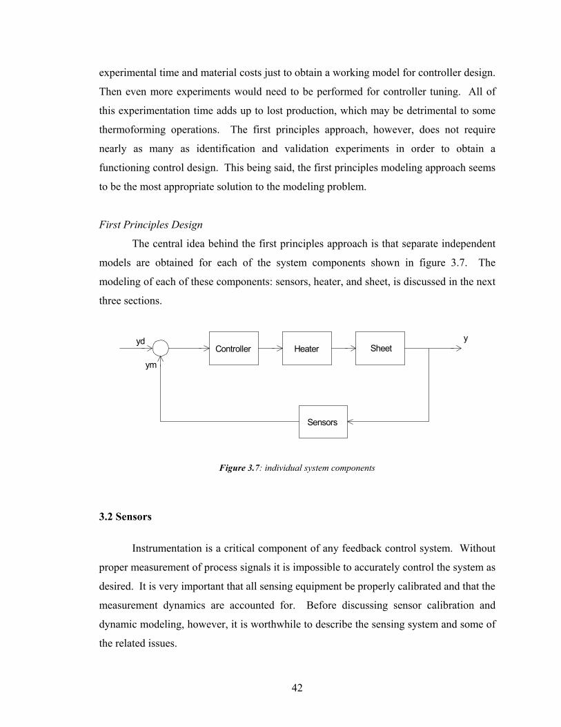
42
experimental time and material costs just to obtain a working model for controller design.
Then even more experiments would need to be performed for controller tuning. All of
this experimentation time adds up to lost production, which may be detrimental to some
thermoforming operations. The first principles approach, however, does not require
nearly as many as identification and validation experiments in order to obtain a
functioning control design. This being said, the first principles modeling approach seems
to be the most appropriate solution to the modeling problem.
First Principles Design
The central idea behind the first principles approach is that separate independent
models are obtained for each of the system components shown in figure 3.7. The
modeling of each of these components: sensors, heater, and sheet, is discussed in the next
three sections.
Controller Heater Sheet
Sensors
y
ym
yd
Figure 3.7: individual system components
3.2 Sensors
Instrumentation is a critical component of any feedback control system. Without
proper measurement of process signals it is impossible to accurately control the system as
desired. It is very important that all sensing equipment be properly calibrated and that the
measurement dynamics are accounted for. Before discussing sensor calibration and
dynamic modeling, however, it is worthwhile to describe the sensing system and some of
the related issues.
43
3.2.1 Thermoforming Instrumentation
Numerous instrumentation and control devices can be found on modern
thermoforming machines. There are, however, only three measurements available for in-
cycle temperature control that are of importance. These are: sheet surface temperature,
oven air temperature, and heater temperature. It is also possible to incorporate airflow
measurements in and around the oven using a hot wire anemometer, but airflow
instrumentation tends to be very complex and fragile, attributes that are not well suited
for industrial applications. Furthermore, the cost of airflow instrumentation, and the
amount of time required to develop an advanced control scheme that incorporates airflow
measurements, does not justify its use. A more practical approach is to limit airflow in
and around the thermoforming equipment.
The heater temperatures are obtained using thermocouples that are embedded into
the ceramic material by the manufacturer. Heater temperature measurements are
integrated into the heater modeling procedure so no further discussion is necessary here.
The oven air temperature measurements can be found using either RTD’s
(Resistance Temperature Detectors) or thermocouples. RTD’s are generally much more
reliable and are used more often in harsh industrial environments. They are also quite
accurate (usually within +/- 1 oC). They also have the advantage of the capability of
being used in applications where the actual sensing element and sensing electronics are
separated by long distances. RTD’s are, however, quite expensive. Thermocouples, on
the other hand, are cheaper, less accurate (+/- 1 oC at best), and they are more difficult to
install. Care must be taken to ensure that the installation is not susceptible to electrical
noise since thermocouple signal levels are very small.
After examining the pros and cons of each type of device the thermocouple was
chosen for the IMI machine because of its low cost and slightly faster response. The use
of a thermocouple for oven air temperature measurements is not automatic. The
measurement is complicated by the fact that the thermocouple is within a radiation
environment and is susceptible to heating from the heater elements, which would result in
erroneous measurements. Two solutions are possible. The first is to limit the radiation
heating effects by coating the thermocouple with a low emissivity, reflective paint. The
44
second approach is to use a sheathed sensor. This was accomplished at IMI by placing
the thermocouples within small lengths of aluminum tubing open at both ends to allow air
movement around the sensor. Pre-fabricated thermocouples with perforated sheathing
are also commercially available.
Sensor placement is also an issue. The IMI setup consisted of two thermocouples
for oven air temperature measurement, one above the sheet and one below. Each sensor
was located at the center of the sheet midway between the heater elements and the sheet.
The number of sensors and their placement will depend on the thermoforming equipment
because the oven air temperature can be highly non-uniform as was reported by Yousefi
in [15].
The sheet surface temperatures are found using non-contact IR (infrared) sensors.
A number of different IR sensor types are commercially available and their cost and
complexity can vary. See table 3.2 for cost comparisons. The simplest design is
commonly referred to as an IR thermocouple. The sensing element receives IR energy
from the measurement target and transforms this energy into a standard thermocouple
voltage signal. This type of sensor costs as little as $200 and it requires no external
power supply since there are no “on board” electronics. The actual temperature
measurement is obtained using separate instrumentation such as a digital multi-meter
configured for thermocouple measurements. The repeatability and interchangeability of
IR thermocouples is similar to regular thermocouples. Other more sophisticated IR
sensors contain their own electronics and can allow the user to specify the emissivity of
the target and configure the output signal to be in the form of an RS-232, 0-5 V, or 4 – 20
mA signal. Most IR sensors require an air-cooling jacket for operation in elevated
temperature environments such as in an oven of a thermoforming machine; however,
some models are configured with a remote pick-up element connected to the main sensor
unit via a fiber optic cable. These types of sensors can be operated in very harsh
environments. The IR sensors that were used for the IMI setup were the Raytek RAY-
MID 10-4 IR sensors which cost approximately $1200 each. They can be configured to
output various thermocouple signals as well as a standard 4-20 mA signal.
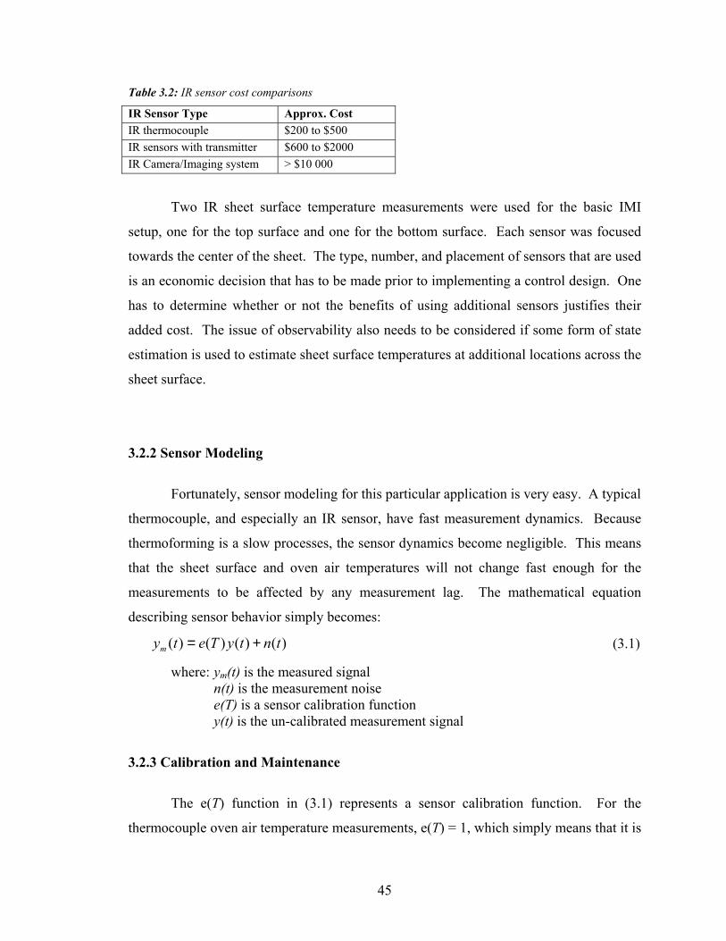
45
Table 3.2: IR sensor cost comparisons IR Sensor Type Approx. Cost IR thermocouple $200 to $500 IR sensors with transmitter $600 to $2000 IR Camera/Imaging system > $10 000
Two IR sheet surface temperature measurements were used for the basic IMI
setup, one for the top surface and one for the bottom surface. Each sensor was focused
towards the center of the sheet. The type, number, and placement of sensors that are used
is an economic decision that has to be made prior to implementing a control design. One
has to determine whether or not the benefits of using additional sensors justifies their
added cost. The issue of observability also needs to be considered if some form of state
estimation is used to estimate sheet surface temperatures at additional locations across the
sheet surface.
3.2.2 Sensor Modeling
Fortunately, sensor modeling for this particular application is very easy. A typical
thermocouple, and especially an IR sensor, have fast measurement dynamics. Because
thermoforming is a slow processes, the sensor dynamics become negligible. This means
that the sheet surface and oven air temperatures will not change fast enough for the
measurements to be affected by any measurement lag. The mathematical equation
describing sensor behavior simply becomes:
( ) ( ) ( ) ( )my t e T y t n t= + (3.1)
where: ym(t) is the measured signal n(t) is the measurement noise e(T) is a sensor calibration function y(t) is the un-calibrated measurement signal
3.2.3 Calibration and Maintenance
The e(T) function in (3.1) represents a sensor calibration function. For the
thermocouple oven air temperature measurements, e(T) = 1, which simply means that it is
46
assumed that the thermocouple is properly calibrated and the only source of error is the
measurement noise n(t).
Unfortunately the IR measurement is not so straightforward. IR sensors are
typically calibrated by the manufacture using a precision controlled, black body
temperature source. The user can then make adjustments to account for the emissivity of
the target area at hand. This works well for most applications but thermoforming is
somewhat of a special case in which there are many different sources for measurement
error. First, most IR sensors are accurate only within a relatively small temperature
range. Thermoforming requires accurate measurements over a wide range of
approximately 25 to 200 oC. Measurement error is then unavoidable if the sensor is
called upon to operate outside of its operating range. Emissivity of polymer materials
changes with temperature, which will also result in measurement errors since almost all
IR sensor models assume a constant emissivity. Changes in ambient air temperature may
affect the electronics in less expensive models and result in further measurement error.
Reflected radiation from the heater elements is probably the most significant source of
measurement error however. Many of the models do have optical lenses, which are
intended to filter out any ambient radiation sources. Nevertheless, additional radiation
will be picked up by the sensor and cause measurement error. Further complicating the
situation is sheet sag, which will cause the level of reflected radiation to change as the
shape of the sheet surface changes.
Given all of the possible sources for measurement error, the only way to properly
calibrate the sensors is to use thermocouples as a true reference temperature. Thin foil
thermocouples were adhered to the sheet surface with a flexible, highly conductive
silicone paste and a strip of high temperature adhesive tape. The temperature dependant
calibration function, e(T), is in the form of a polynomial and is written as:
/( ) T C
sensor
Te TT
= (3.2)
where: TT/C is the thermocouple measurement
Tsensor is the IR sensor measurement
47
It is important to note that proper bonding between the sheet surface and the foil
thermocouple is essential. Thermocouple cement is not appropriate for bonding the
thermocouple to the sheet surface because the cement hardens and becomes rigid. As the
sheet sags the bonded thermocouple will actually begin to pull away from the sheet
surface, and the thermocouple measurement will not reflect the true surface temperature,
thus resulting in improper calibration.
Proper instrument maintenance is key in maintaining the performance level of any
control system. The IR sensors will need to be periodically recalibrated. The
maintenance schedule would depend upon the factory specifications for the particular
sensor model that is being used. Ideally, the sensors should be recalibrated before the
start of every new production run using the procedure described above.
3.3 Heater Modeling
The purpose of the heater modeling is to capture the dynamic behavior of the
heater elements. As mentioned in the process description, there are many different kinds
of heating systems available for thermoforming. The IMI machine uses ceramic heating
elements to heat the sheet. The basic structure and dimensions of these elements are
shown in figure 3.8. The actual resistive heating element is a thin wire that is embedded
in the ceramic material. The purpose of the ceramic material is to create a stable,
relatively even temperature source.
Since the geometry of the heaters is quite complex, it would be extremely difficult
to develop an analytical model for the heaters. Furthermore, the material properties are
not well known, and the exact positions of the heating coil and embedded thermocouple
are unknown. It is, therefore, not reasonable to use a first principles approach for heater
modeling. Unlike the heater-sheet combination, the black box approach is well suited for
heater modeling since standard system identification techniques can be applied. A
number of different system identification experiments were performed for the heater
modeling. Figures 3.9 and 3.10 will be used to explain the heater modeling methodology.
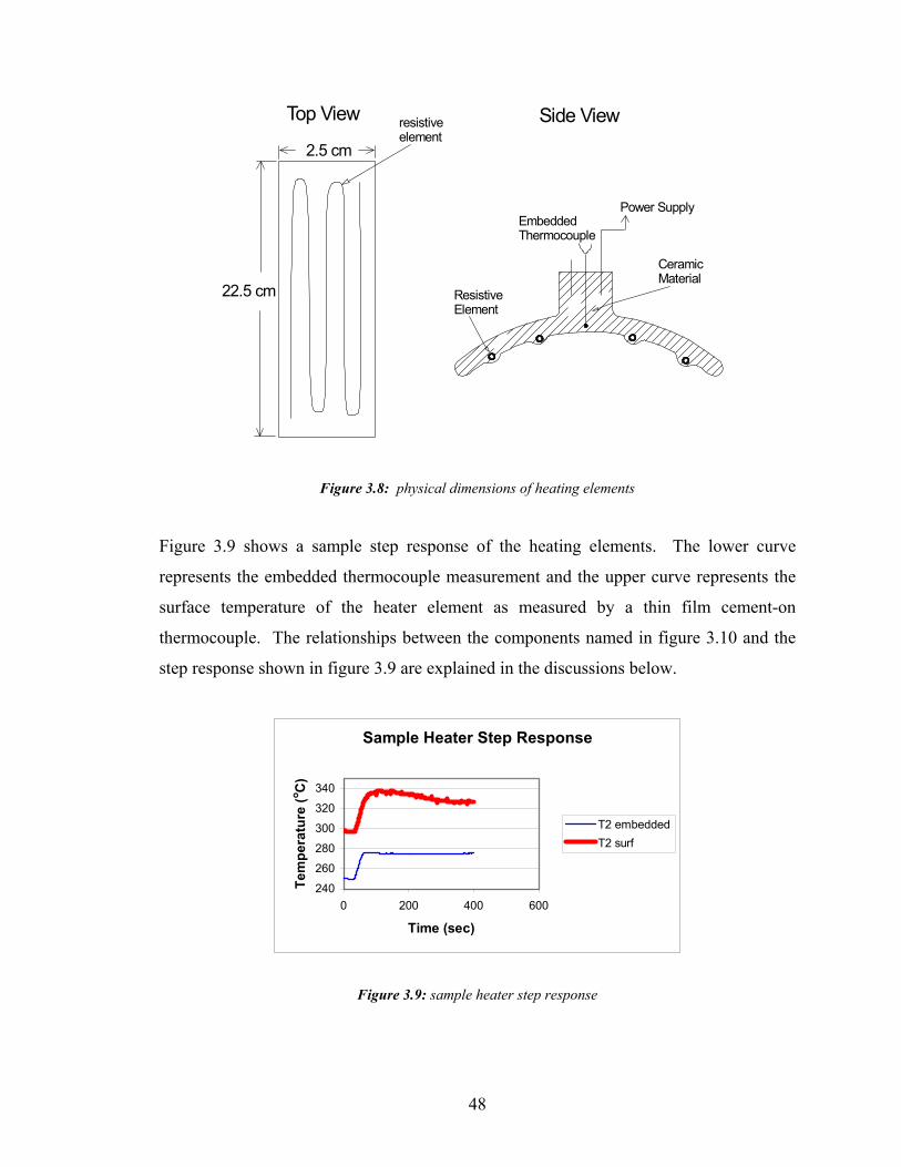
48
2.5 cm
22.5 cm
Top View resistive element
Side View
Power SupplyEmbedded Thermocouple
ResistiveElement
CeramicMaterial
Figure 3.8: physical dimensions of heating elements
Figure 3.9 shows a sample step response of the heating elements. The lower curve
represents the embedded thermocouple measurement and the upper curve represents the
surface temperature of the heater element as measured by a thin film cement-on
thermocouple. The relationships between the components named in figure 3.10 and the
step response shown in figure 3.9 are explained in the discussions below.
Sample Heater Step Response
240260280300320340
0 200 400 600
Time (sec)
Tem
pera
ture
(o C)
T2 embeddedT2 surf
Figure 3.9: sample heater step response
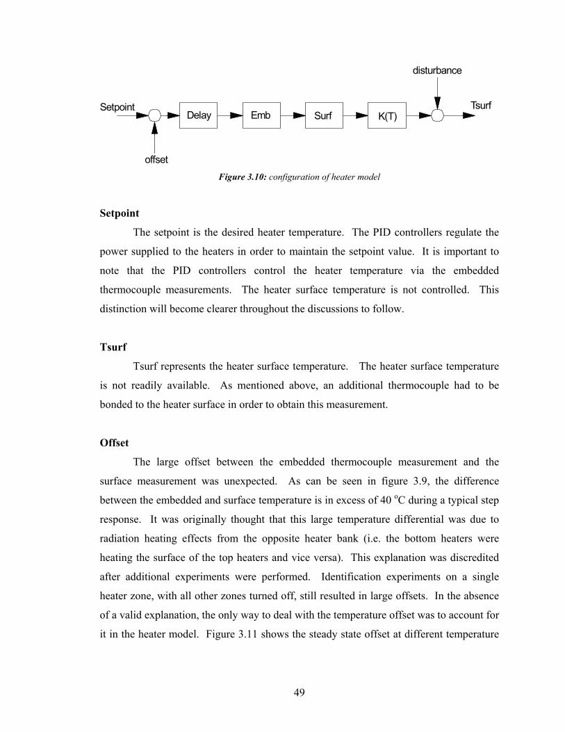
49
Delay Emb Surf K(T)
disturbance
offset
Setpoint Tsurf
Figure 3.10: configuration of heater model
Setpoint
The setpoint is the desired heater temperature. The PID controllers regulate the
power supplied to the heaters in order to maintain the setpoint value. It is important to
note that the PID controllers control the heater temperature via the embedded
thermocouple measurements. The heater surface temperature is not controlled. This
distinction will become clearer throughout the discussions to follow.
Tsurf
Tsurf represents the heater surface temperature. The heater surface temperature
is not readily available. As mentioned above, an additional thermocouple had to be
bonded to the heater surface in order to obtain this measurement.
Offset
The large offset between the embedded thermocouple measurement and the
surface measurement was unexpected. As can be seen in figure 3.9, the difference
between the embedded and surface temperature is in excess of 40 oC during a typical step
response. It was originally thought that this large temperature differential was due to
radiation heating effects from the opposite heater bank (i.e. the bottom heaters were
heating the surface of the top heaters and vice versa). This explanation was discredited
after additional experiments were performed. Identification experiments on a single
heater zone, with all other zones turned off, still resulted in large offsets. In the absence
of a valid explanation, the only way to deal with the temperature offset was to account for
it in the heater model. Figure 3.11 shows the steady state offset at different temperature
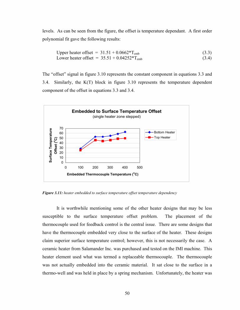
50
levels. As can be seen from the figure, the offset is temperature dependant. A first order
polynomial fit gave the following results:
Upper heater offset = 31.51 + 0.0662*Temb (3.3) Lower heater offset = 35.51 + 0.04252*Temb (3.4) The “offset” signal in figure 3.10 represents the constant component in equations 3.3 and
3.4. Similarly, the K(T) block in figure 3.10 represents the temperature dependent
component of the offset in equations 3.3 and 3.4.
Embedded to Surface Temperature Offset(single heater zone stepped)
010203040506070
0 100 200 300 400 500
Embedded Thermocouple Temperature (oC)
Surf
ace
Tem
pera
ture
O
ffset
(o C)
Bottom HeaterTop Heater
Figure 3.11: heater embedded to surface temperature offset temperature dependency
It is worthwhile mentioning some of the other heater designs that may be less
susceptible to the surface temperature offset problem. The placement of the
thermocouple used for feedback control is the central issue. There are some designs that
have the thermocouple embedded very close to the surface of the heater. These designs
claim superior surface temperature control; however, this is not necessarily the case. A
ceramic heater from Salamander Inc. was purchased and tested on the IMI machine. This
heater element used what was termed a replaceable thermocouple. The thermocouple
was not actually embedded into the ceramic material. It sat close to the surface in a
thermo-well and was held in place by a spring mechanism. Unfortunately, the heater was
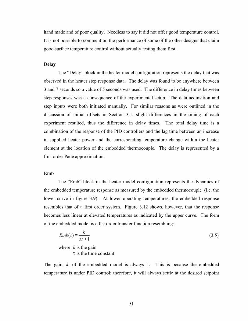
51
hand made and of poor quality. Needless to say it did not offer good temperature control.
It is not possible to comment on the performance of some of the other designs that claim
good surface temperature control without actually testing them first.
Delay
The “Delay” block in the heater model configuration represents the delay that was
observed in the heater step response data. The delay was found to be anywhere between
3 and 7 seconds so a value of 5 seconds was used. The difference in delay times between
step responses was a consequence of the experimental setup. The data acquisition and
step inputs were both initiated manually. For similar reasons as were outlined in the
discussion of initial offsets in Section 3.1, slight differences in the timing of each
experiment resulted, thus the difference in delay times. The total delay time is a
combination of the response of the PID controllers and the lag time between an increase
in supplied heater power and the corresponding temperature change within the heater
element at the location of the embedded thermocouple. The delay is represented by a
first order Pade; approximation.
Emb
The “Emb” block in the heater model configuration represents the dynamics of
the embedded temperature response as measured by the embedded thermocouple (i.e. the
lower curve in figure 3.9). At lower operating temperatures, the embedded response
resembles that of a first order system. Figure 3.12 shows, however, that the response
becomes less linear at elevated temperatures as indicated by the upper curve. The form
of the embedded model is a fist order transfer function resembling:
( )1
kEmb ssτ
=+
(3.5)
where: k is the gain τ is the time constant The gain, k, of the embedded model is always 1. This is because the embedded
temperature is under PID control; therefore, it will always settle at the desired setpoint
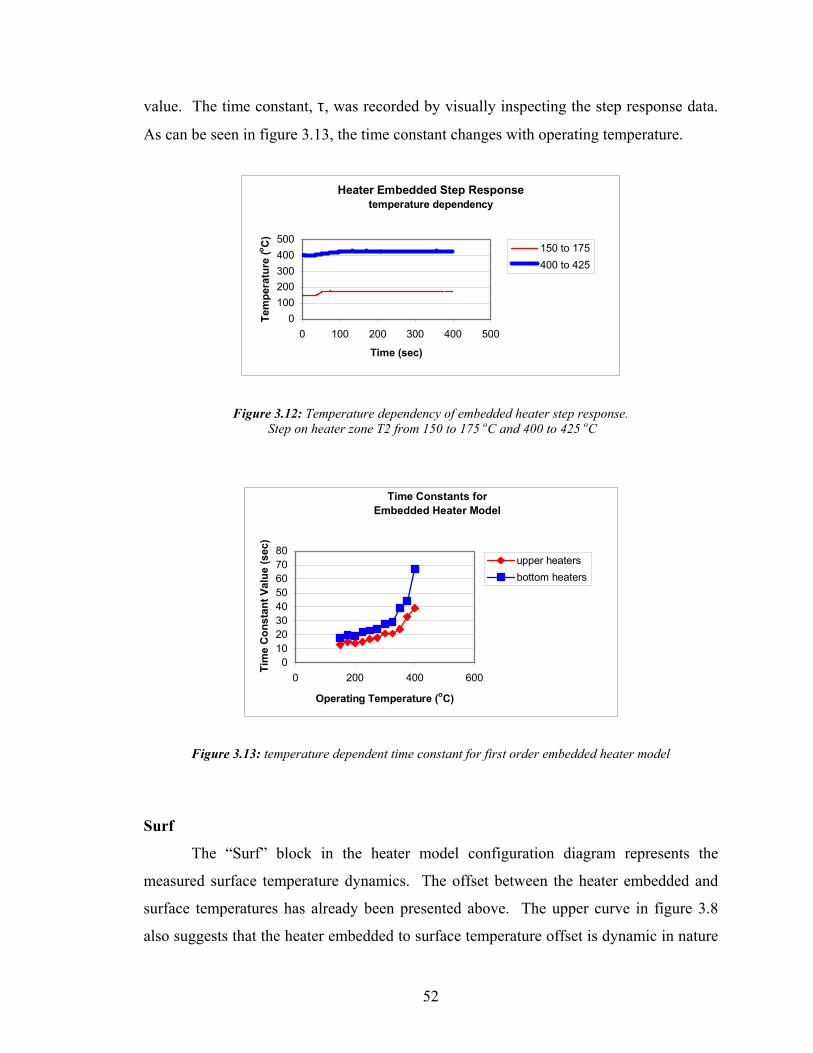
52
value. The time constant, τ, was recorded by visually inspecting the step response data.
As can be seen in figure 3.13, the time constant changes with operating temperature.
Heater Embedded Step Responsetemperature dependency
0100200300400500
0 100 200 300 400 500
Time (sec)
Tem
pera
ture
(o C)
150 to 175400 to 425
Figure 3.12: Temperature dependency of embedded heater step response. Step on heater zone T2 from 150 to 175 oC and 400 to 425 oC
Time Constants for Embedded Heater Model
01020304050607080
0 200 400 600
Operating Temperature (oC)
Tim
e C
onst
ant V
alue
(sec
)
upper heatersbottom heaters
Figure 3.13: temperature dependent time constant for first order embedded heater model
Surf
The “Surf” block in the heater model configuration diagram represents the
measured surface temperature dynamics. The offset between the heater embedded and
surface temperatures has already been presented above. The upper curve in figure 3.8
also suggests that the heater embedded to surface temperature offset is dynamic in nature
53
as evidenced by the overshoot in the surface temperature response. The first attempt to
capture the surface temperature dynamics involved visually inspecting the step response
data to obtain the parameters for a second order model of the following form:
1 0
22 1 0
( )surfa s aT s
b s b s b+=
+ + (3.6)
Unfortunately, the results were not satisfactory. The second approach employed
Matlab’s system identification toolbox. An appropriate model was obtained using the
input-output (heater embedded and surface temperatures respectively) data from the step
experiments. A number of different model structures were applied with the best
performance given by a second order state space model3.
The application of the system identification methods was not immediately
successful. Various data conditioning steps needed to be performed first. The first step
was to normalize the input and output data. This was accomplished by subtracting the
initial value of each data set from the remaining values in the corresponding data set.
This resulted in initial input and output values of zero. Next, the time delay was removed
from the step response data, and then outliers were removed. Finally, the temperature
dependant offset between the embedded and surface temperatures was removed from the
output (surface temperature) data. When combined, these conditioning operations led to
good system identification results.
One block is omitted from figure 3.10 in order to avoid confusion. This block is
the PID controller. The PID controller is actually embedded in the ‘Emb’ block of the
heater model, because the input-output data that was used for the system identification
was the actual closed loop response of the heater elements. In effect, the heater model
captures the dynamics of the heater elements as well as the closed loop PID control. This
configuration was used because the relationship between applied heater power and heater
temperature is highly nonlinear and not well known. Separation of the PID controller and
heater dynamics is unnecessary as it does not add any value to the design. Such a
separation would also be quite difficult and introduce added complexity. 3 All model parameters are given in the Appendix.
54
3.3.1 Disturbances and Modeling Errors
Although a detailed study of disturbances acting on the heater system was not
performed, it is worthwhile mentioning the important disturbance sources. One of the
main sources of heater disturbances is air movement in and around the oven. Any cooler
air that enters the oven area will pass over the heater surfaces, which will have a cooling
effect. There is also air movement within the oven during a regular heating cycle caused
by natural convection currents within the oven. The fact that hot air rises is well known.
This suggests that the effects from air movement will be different for the upper and lower
ovens respectively. Furthermore, it is extremely difficult to predict airflow within the
oven. The only reasonable way to predict airflow within the oven and capture its effects
on heater temperature is through the use of artificial neural networks. This approach to
disturbance modeling would, however, require time and a significant amount of
experimental data to train the neural network. It is for these reasons that disturbance
modeling was not considered in this project.
Another source of heater disturbance is supply voltage fluctuations. A power
source with higher frequency fluctuations, or higher order harmonic content, will not
adversely affect heater performance. This is accomplished without the addition of any
power regulation electronics. The high thermal mass of the ceramic material naturally
results in a low bandwidth; therefore, higher frequency disturbances will be easily
attenuated. Very low frequency fluctuations on the other hand, can affect heater
temperatures. Since these types of disturbances are actually power quality issues and
beyond the scope of this thesis, no further investigation into power supply related
disturbances was made.
It is also important to identify modeling errors and future improvements that can
be made. The major source for modeling error is the fact that the temperature across the
surface of the heaters was found to be very uneven. Measured temperature differences
across the surface are in excess of 50 oC for some individual heater elements. This
automatically becomes a source for modeling error since the heater models were found
using measured input-output data. The output data, heater surface temperature, was
recorded using a small, cement on thermocouple, which for all intents and purposes is a
55
point source measurement that does not reflect the true average surface temperature of
the heater. An attempt was made to assess the accuracy of the measured output data
using thermal images of the heater elements taken with an IR camera. The images were
not consistent enough, however, to make a proper assessment, or adjustment, of the
output data. As a result, the large surface temperature differentials were simply treated as
an uncertainty for controller design.
An important fact that was discovered only towards the very end of this project is
that the voltage level supplied to the heaters was incorrect. The heaters were operated
under a 208 VAC supply upon completion of this project. At this voltage level,
temperature differentials in excess of 50 oC were measured across the heater surface. It
was later learned that the heaters were supposed to be operated at 240 VAC. A test was
performed in which 240 VAC was supplied to a single heater element and the
temperature differential across the heater was measured to be less than 10 oC. Modeling
error would be greatly reduced if new heaters were used of if the existing heaters were
operated at their specified voltage levels. Unfortunately, time and economic constraints
meant that results for this project were obtained using these very uncertain heater
elements. More importantly, however, is the fact that the overall heater modeling
methodology presented here can be applied to any thermoforming oven using electrical
radiant heaters.
3.3.2 Model Validation After constructing the overall heater model from its individual components, the
heater model was validated using experimental data that was different from the original
data that was used to identify the model components. Figure 3.14 shows that the model
performs quite well over a wide temperature range. Figure 3.15 shows the response of
the heater model, found using step response data for heater zone T2, against experimental
data for a step test on heater zone B2. The plots suggest that a single model can be used
to describe the behavior of both the upper and lower heater banks. For simplicity, a
single heater model was used, but separate models for the upper and lower heaters,
respectively, could be used if desired.
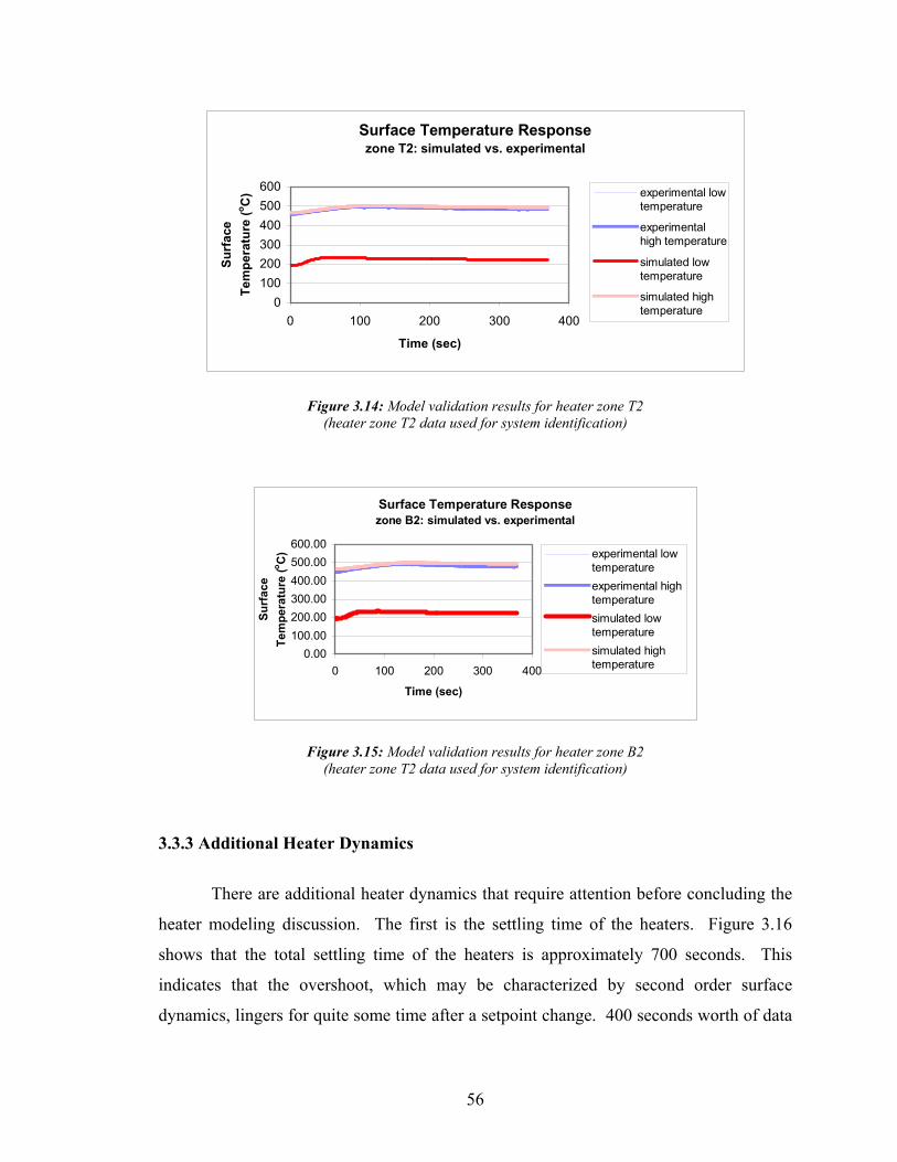
56
Surface Temperature Responsezone T2: simulated vs. experimental
0100200300400500600
0 100 200 300 400
Time (sec)
Surf
ace
Tem
pera
ture
(o C) experimental low
temperature
experimentalhigh temperature
simulated lowtemperature
simulated hightemperature
Figure 3.14: Model validation results for heater zone T2 (heater zone T2 data used for system identification)
Surface Temperature Responsezone B2: simulated vs. experimental
0.00100.00200.00300.00400.00500.00600.00
0 100 200 300 400
Time (sec)
Surf
ace
Tem
pera
ture
(o C) experimental low
temperatureexperimental hightemperaturesimulated lowtemperaturesimulated hightemperature
Figure 3.15: Model validation results for heater zone B2 (heater zone T2 data used for system identification)
3.3.3 Additional Heater Dynamics
There are additional heater dynamics that require attention before concluding the
heater modeling discussion. The first is the settling time of the heaters. Figure 3.16
shows that the total settling time of the heaters is approximately 700 seconds. This
indicates that the overshoot, which may be characterized by second order surface
dynamics, lingers for quite some time after a setpoint change. 400 seconds worth of data

57
was collected for the system identification experiments. As a guideline, this should be
the minimum amount of time used for system identification of ceramic heating elements.
Settling Time
0100200300400
0 500 1000 1500 2000
Time (sec)
Tem
pera
ture
(o C)
B2 embB2 surfT2 embT2 surf
Figure 3.16: Heater settling time The coupling between heater zones was also examined as part of the heater
modeling procedure. It was assumed that all heater zones were decoupled from one
another. In other words, the assumption is that a change in setpoint in one zone does not
affect the temperature of any of the remaining zones. This is an important assumption.
Any significant coupling between heating zones, the actuators, would make multivariable
control of the sheet temperature extremely difficult. After reviewing the results shown in
figure 3.17, it was decided that the decoupling assumption was valid. The plot was
obtained under the following experimental conditions:
1) heater zones T2 and B2 were held at a setpoint of 200 oC
2) all other remaining zones in the oven were stepped from room temperature to
400 oC
As can be seen from the figure the effects on heater zones T2 and B2 are relatively small
under the conditions of extreme temperature differentials between heater zones. Under
normal operating conditions, the temperature differentials between heater zones will be
much less; therefore, the decoupled assumption holds.
The most significant aspect of the heater dynamics can be observed by viewing
the negative step response shown in figure 3.18. The shallow slope of the curves in the
figure indicates that heater cooling is much slower than heating. This is true because the
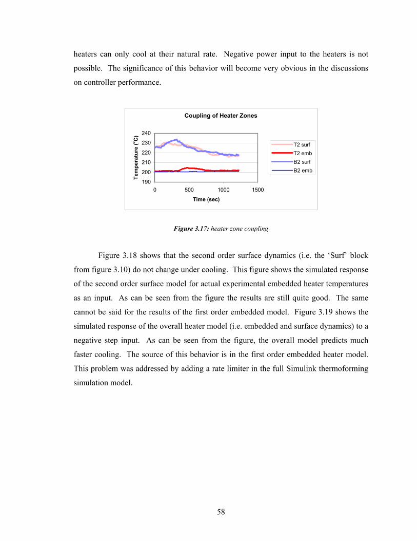
58
heaters can only cool at their natural rate. Negative power input to the heaters is not
possible. The significance of this behavior will become very obvious in the discussions
on controller performance.
Coupling of Heater Zones
190
200
210
220
230
240
0 500 1000 1500
Time (sec)
Tem
pera
ture
(o C)
T2 surfT2 embB2 surfB2 emb
Figure 3.17: heater zone coupling
Figure 3.18 shows that the second order surface dynamics (i.e. the ‘Surf’ block
from figure 3.10) do not change under cooling. This figure shows the simulated response
of the second order surface model for actual experimental embedded heater temperatures
as an input. As can be seen from the figure the results are still quite good. The same
cannot be said for the results of the first order embedded model. Figure 3.19 shows the
simulated response of the overall heater model (i.e. embedded and surface dynamics) to a
negative step input. As can be seen from the figure, the overall model predicts much
faster cooling. The source of this behavior is in the first order embedded heater model.
This problem was addressed by adding a rate limiter in the full Simulink thermoforming
simulation model.
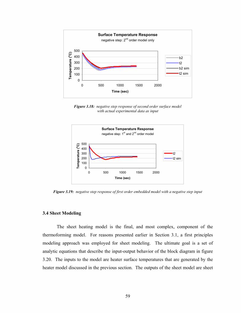
59
Surface Temperature Responsenegative step: 2nd order model only
0
100
200
300
400
500
0 500 1000 1500 2000
Time (sec)
Tem
pera
ture
(o C)
b2t2b2 simt2 sim
Figure 3.18: negative step response of second order surface model with actual experimental data as input
Surface Temperature Responsenegative step: 1st and 2nd order model
0100200300400500
0 500 1000 1500 2000
Time (sec)
Tem
pera
ture
(o C)
t2t2 sim
Figure 3.19: negative step response of first order embedded model with a negative step input
3.4 Sheet Modeling
The sheet heating model is the final, and most complex, component of the
thermoforming model. For reasons presented earlier in Section 3.1, a first principles
modeling approach was employed for sheet modeling. The ultimate goal is a set of
analytic equations that describe the input-output behavior of the block diagram in figure
3.20. The inputs to the model are heater surface temperatures that are generated by the
heater model discussed in the previous section. The outputs of the sheet model are sheet
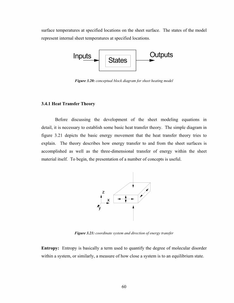
60
surface temperatures at specified locations on the sheet surface. The states of the model
represent internal sheet temperatures at specified locations.
StatesInputs Outputs
Figure 3.20: conceptual block diagram for sheet heating model
3.4.1 Heat Transfer Theory
Before discussing the development of the sheet modeling equations in
detail, it is necessary to establish some basic heat transfer theory. The simple diagram in
figure 3.21 depicts the basic energy movement that the heat transfer theory tries to
explain. The theory describes how energy transfer to and from the sheet surfaces is
accomplished as well as the three-dimensional transfer of energy within the sheet
material itself. To begin, the presentation of a number of concepts is useful.
z
y
x
Figure 3.21: coordinate system and direction of energy transfer
Entropy: Entropy is basically a term used to quantify the degree of molecular disorder
within a system, or similarly, a measure of how close a system is to an equilibrium state.
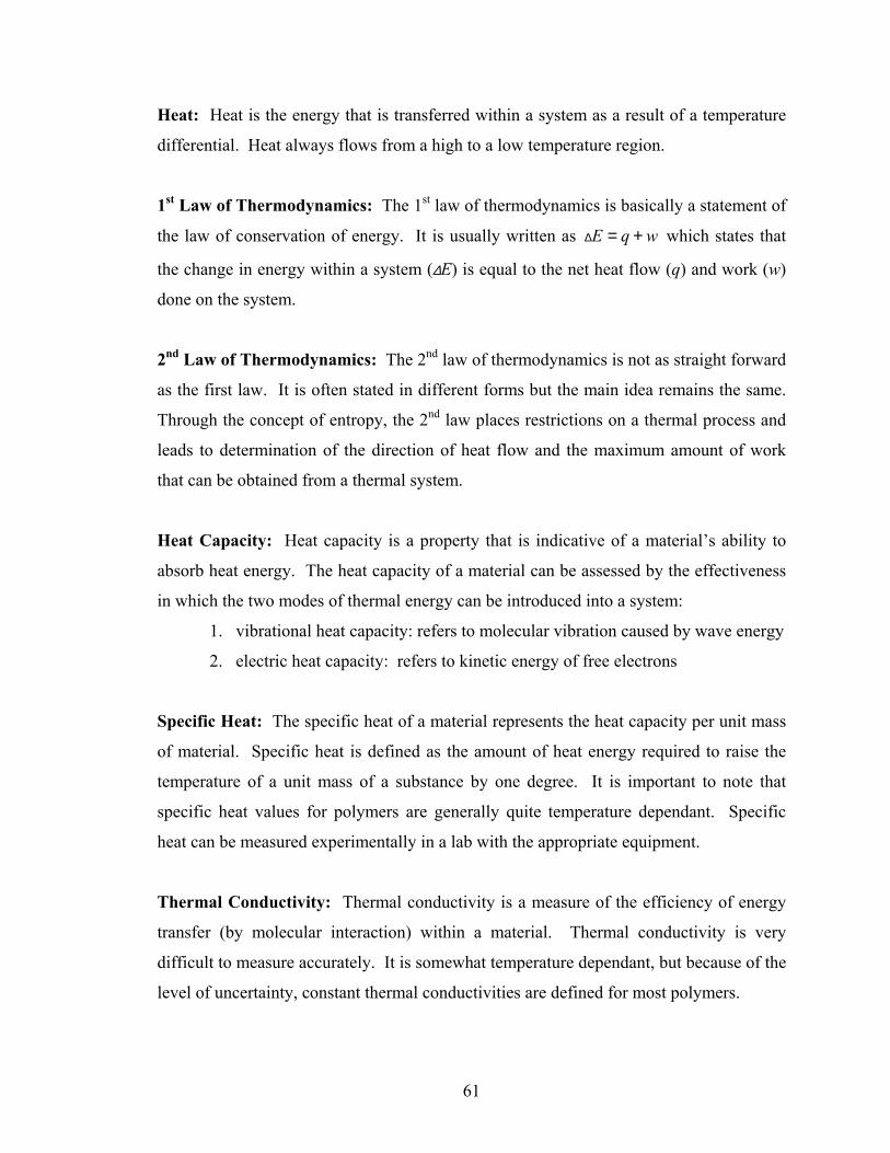
61
Heat: Heat is the energy that is transferred within a system as a result of a temperature
differential. Heat always flows from a high to a low temperature region.
1st Law of Thermodynamics: The 1st law of thermodynamics is basically a statement of
the law of conservation of energy. It is usually written as E q w∆ = + which states that
the change in energy within a system (∆E) is equal to the net heat flow (q) and work (w)
done on the system.
2nd Law of Thermodynamics: The 2nd law of thermodynamics is not as straight forward
as the first law. It is often stated in different forms but the main idea remains the same.
Through the concept of entropy, the 2nd law places restrictions on a thermal process and
leads to determination of the direction of heat flow and the maximum amount of work
that can be obtained from a thermal system.
Heat Capacity: Heat capacity is a property that is indicative of a material’s ability to
absorb heat energy. The heat capacity of a material can be assessed by the effectiveness
in which the two modes of thermal energy can be introduced into a system:
1. vibrational heat capacity: refers to molecular vibration caused by wave energy
2. electric heat capacity: refers to kinetic energy of free electrons
Specific Heat: The specific heat of a material represents the heat capacity per unit mass
of material. Specific heat is defined as the amount of heat energy required to raise the
temperature of a unit mass of a substance by one degree. It is important to note that
specific heat values for polymers are generally quite temperature dependant. Specific
heat can be measured experimentally in a lab with the appropriate equipment.
Thermal Conductivity: Thermal conductivity is a measure of the efficiency of energy
transfer (by molecular interaction) within a material. Thermal conductivity is very
difficult to measure accurately. It is somewhat temperature dependant, but because of the
level of uncertainty, constant thermal conductivities are defined for most polymers.

62
Thermal Diffusivity: Thermal diffusivity is similar to conductivity in some respects.
Thermal conductivity can be considered to be a measure of the extent of energy
transmission through a substance whereas thermal diffusivity is a measure of the rate at
which the energy transfer occurs.
Thermal Expansion Coefficient: The thermal expansion coefficient is a measure of
how much a material will expand when heated. One of the main causes for expansion of
polymers is the temperature dependency of the material’s density.
Infrared Spectra: Infrared spectra refers to the fact that polymers tend to selectively
absorb, transmit, and reflect radiation energy of different wavelengths. This project used
relatively thick, opaque materials, and it was assumed that all of the radiation energy was
absorbed by the material (i.e. no reflection/transmission). This is not the case with all
materials and spectral response can be an important thermoforming issue. Transmission
spectra for various polymers are given in [1].
Heating Mechanisms
There are three energy exchange mechanisms involved in the thermoforming
process: conduction, convection, and radiation.
Conduction
The conduction heating mechanism is a solid phase heat transfer phenomenon that
occurs within a solid body or between two bodies in contact with one another. The
energy transfer, or heat flow, occurs as a result of the transfer of vibrational molecular
wave energy as well as the movement of free electrons within a body. Conduction heat
transfer is governed by Fourier’s Law, which states that energy transfer occurs when
temperature gradients exist within a body, and that the rate of energy transfer is
proportional to the normal of the temperature gradient. Fourier’s Law can be written as:
q dkA dx
θ= − (3.7)
where q/A is the heat flow rate per unit area
63
k is the thermal conductivity
ddxθ is the temperature (θ) gradient in the direction of heat flow, x
The general three-dimensional heat conduction equation can be written in Cartesian
coordinates as:
2 2 2
2 2 2
1d d d q ddx dy dz k dt
θ θ θ θα
+ + + = (3.8)
where 2 2 2
2 2 2
d d ddx dy dz
θ θ θ+ + represents the temperature gradients within the body
qk
is a term that represents any energy that may be generated internally
within the body
α is the thermal diffusivity
ddtθ is the time rate of change in temperature within the body
Equation (3.8) describes the temperature distribution within a body over time. Solving
this equation requires several boundary conditions. Two of the boundary conditions are
governed by the two remaining heat transfer mechanisms: convection and radiation.
Convection
Convection is a fluid phase contact heat transfer mechanism. For thermoforming,
this means that energy is transferred between the sheet surface and a thin fluid (air) layer
above the sheet surface. It is important to note that convection heat transfer is actually a
conduction process. At the sheet surface, the velocity of the air surrounding the sheet is
zero, and the energy transfer is between the sheet surface and stationary air molecules in
contact with the sheet surface. The net rate of heat flow is given by the equation:
( )sheetq hA
θ θ∞= − (3.9)
where q/A is the flow rate per unit area
θ∞ is the temperature of the air surrounding the sheet
θsheet is the sheet surface temperature
h is the convection heat transfer coefficient
64
At first glance, equation (3.9) looks very similar to Fourier’s Law. As mentioned above,
the similarity is because convection is actually a conduction process. The differences lie
with the proportionality constants k and h. In Fourier’s Law, k, is more or less a constant
for most polymers. The convection heat transfer coefficient, h, in equation (3.9) is
dependent upon many variables including the thermal properties of the fluid (thermal
conductivity, specific heat, density, etc.) and the viscous behavior of the fluid. The fact
that the viscous behavior of the fluid affects the heat transfer is evidenced by the fact that
fast moving air over the sheet surface will have a greater impact on the sheet surface
temperature than will slow moving, or quiescent air.
It is important to mention the direction of heat flow as a result of the notation in
equation (3.9). A typical thermoforming application will see a reversal in convection
heat transfer over the heating period. At the beginning of the heating cycle, the oven air
temperature will usually be greater than the sheet surface temperature. The air movement
around the sheet will then tend to heat the sheet during the beginning of the cycle.
Towards the end of the heating cycle, the sheet temperature will rise above the oven air
temperature, which increases very little during the heating cycle. At this point, the oven
air movement around the sheet will then begin to cool the sheet rather than heat it.
Radiation
Unlike the previous two heating mechanisms, radiation heat transfer is a non-
contact heat transfer mechanism. Radiation heat transfer is the dominant heating
mechanism in the thermoforming process. Electromagnetic energy is emitted by the oven
heaters and absorbed at the sheet surface. The absorbed energy at the sheet surface is
then conducted towards the center of the sheet. It is important to note that the radiation
energy transfer does not directly depend on the distance between the source (heaters) and
the sink (sheet).
The Stephan-Boltzmann Law of radiation states that the maximum total energy
emitted by an ideal source, termed a black body, is given by the equation:
4bE σθ= (3.10)
where Eb is the radiation energy emitted by the black body
θ is the temperature, in degrees Kelvin, of the black body
65
σ is a proportionality constant called the Stephan-Boltzmann constant
Obviously the concept of a black body is only theoretical. To account for the fact that
realistic temperature to radiation energy conversion efficiency is less than 100 percent,
we need to introduce the concepts of emissivity and absorptivity. Emissivity is a scaling
factor which indicates the fraction of black body radiation emitted by a non-ideal source
called a gray body. Similarly, absorptivity is a scaling factor which indicates the fraction
of radiation absorbed by a gray body as compared to an ideal black body that absorbs all
radiation it is exposed to. In general, emissivities and absorptivities of materials are
considered to be equal. As such, the term emissivity is used interchangeably to describe
both the absorption and emitting properties of a material. Emissivities are usually
wavelength dependant, reflecting the fact that most materials tend to absorb radiant
energy preferentially in specific wavelength ranges of the infrared spectrum. As
mentioned earlier, infrared spectra were not considered in this project.
Using the Stephan –Boltzmann Law, the energy exchange that takes place during
the thermoforming heating cycle is written as:
4 4( )view eff heater sheet
q FA
σ θ θε= − (3.11)
where q/A is the heat flow into the sheet surface per unit area
σ is the Stephan-Boltzmann constant
Fview is the radiation view factor
εeff is the effective emissivity
θheater is the heater surface temperature
θsheet is the sheet surface temperature
As can be seen from the above equation, the energy absorbed by the sheet is proportional
to the difference between the 4th powers of the heater and sheet temperatures. Two new
terms appear in this equation. The first is the effective emissivity (εeff ), or efficiency, of
66
the total energy exchange between the heaters and the sheet. The effective emissivity is a
function of the sheet and heater emissivity values and is calculated using:
1
1 1 1effh sε ε
ε−
= + −
(3.12)
where εheater is the heater emissivity
εsheet is the sheet emissivity
The second new term to appear in equation (3.11) is the radiation view factor (Fview). The
view factor is a dimensionless scaling factor to account for the fact that a body only
absorbs radiation energy that it “sees” from the source. In other words, all of the
radiation energy emitted from a source may not hit the target body; therefore, a fraction
of the radiation energy is lost to the surrounding environment. This lost energy is
accounted for by the radiation view factor. The view factors for this project were
calculated using a formula obtained from a catalogue of view factors for various
geometric configurations.4
3.4.2 Sheet Model
The development of the thermoforming sheet heating model begins with the
generalized three-dimensional conduction equation (3.8). An analytical solution to these
types of three-dimensional partial differential equations is often quite elusive, therefore, a
few simplifying assumptions are required. The first assumption is that the conduction
will only occur through the sheet thickness in the z direction. In other words, it is
assumed the transfer of energy in the x-y direction will be negligible. This assumption is
valid since the temperature gradients across the sheet surface in the x-y direction will be
relatively small as compared with the temperature gradients through the sheet thickness.
Coupled with the fact that thermoplastic materials are generally poor heat conductors, the
dominant energy transfer will occur in the z direction.
4 Consult [5] for generalized view factor calculations
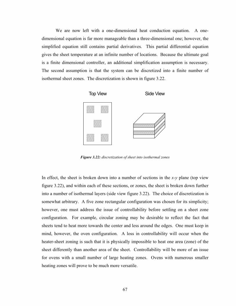
67
We are now left with a one-dimensional heat conduction equation. A one-
dimensional equation is far more manageable than a three-dimensional one; however, the
simplified equation still contains partial derivatives. This partial differential equation
gives the sheet temperature at an infinite number of locations. Because the ultimate goal
is a finite dimensional controller, an additional simplification assumption is necessary.
The second assumption is that the system can be discretized into a finite number of
isothermal sheet zones. The discretization is shown in figure 3.22.
Top View Side View
Figure 3.22: discretization of sheet into isothermal zones
In effect, the sheet is broken down into a number of sections in the x-y plane (top view
figure 3.22), and within each of these sections, or zones, the sheet is broken down further
into a number of isothermal layers (side view figure 3.22). The choice of discretization is
somewhat arbitrary. A five zone rectangular configuration was chosen for its simplicity;
however, one must address the issue of controllability before settling on a sheet zone
configuration. For example, circular zoning may be desirable to reflect the fact that
sheets tend to heat more towards the center and less around the edges. One must keep in
mind, however, the oven configuration. A loss in controllability will occur when the
heater-sheet zoning is such that it is physically impossible to heat one area (zone) of the
sheet differently than another area of the sheet. Controllability will be more of an issue
for ovens with a small number of large heating zones. Ovens with numerous smaller
heating zones will prove to be much more versatile.
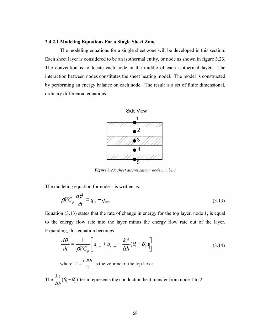
68
3.4.2.1 Modeling Equations For a Single Sheet Zone
The modeling equations for a single sheet zone will be developed in this section.
Each sheet layer is considered to be an isothermal entity, or node as shown in figure 3.23.
The convention is to locate each node in the middle of each isothermal layer. The
interaction between nodes constitutes the sheet heating model. The model is constructed
by performing an energy balance on each node. The result is a set of finite dimensional,
ordinary differential equations.
1
3
4
5
2
Side View
Figure 3.23: sheet discretization: node numbers
The modeling equation for node 1 is written as:
1p in out
dVC q qdtθρ = − (3.13)
Equation (3.13) states that the rate of change in energy for the top layer, node 1, is equal
to the energy flow rate into the layer minus the energy flow rate out of the layer.
Expanding, this equation becomes:
11 2
1 ( ) rad convp
d kAq qdt VC hθ θ θ
ρ = + − − ∆
(3.14)
where 2
2l hV ∆= is the volume of the top layer
The 1 2( )kAh
θ θ−∆
term represents the conduction heat transfer from node 1 to 2.
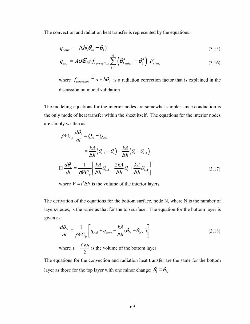
69
The convection and radiation heat transfer is represented by the equations:
conv 1 = A ( )q h θ θ∞ − (3.15)
( )6
4 4 rad 1
1
= i i
eff correction heater viewi
q A f Fσ θ θε=
−∑ (3.16)
where 1correctionf a bθ= + is a radiation correction factor that is explained in the
discussion on model validation
The modeling equations for the interior nodes are somewhat simpler since conduction is
the only mode of heat transfer within the sheet itself. The equations for the interior nodes
are simply written as:
( ) ( )1 1
ip in out
i i i i
dVC Q Qdt
kA kAh h
θρ
θ θ θ θ− +
= −
= − − −∆ ∆
1 11 2 i
i i ip
d kA kA kAdt VC h h hθ θ θ θ
ρ − + ∴ = − + ∆ ∆ ∆
(3.17)
where 2V l h= ∆ is the volume of the interior layers
The derivation of the equations for the bottom surface, node N, where N is the number of
layers/nodes, is the same as that for the top surface. The equation for the bottom layer is
given as:
11 ( ) N
rad conv N Np
d kAq qdt VC hθ θ θ
ρ − = + − − ∆
(3.18)
where 2
2l hV ∆= is the volume of the bottom layer
The equations for the convection and radiation heat transfer are the same for the bottom
layer as those for the top layer with one minor change: 1 Nθ θ= .
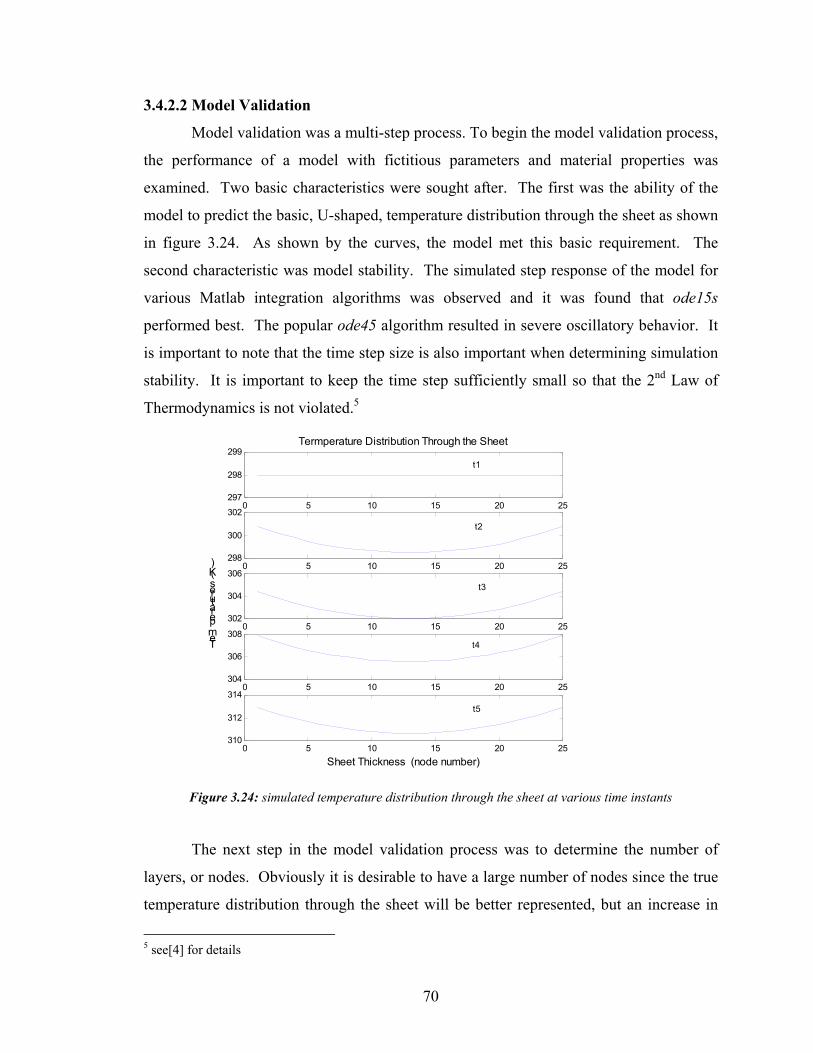
70
3.4.2.2 Model Validation
Model validation was a multi-step process. To begin the model validation process,
the performance of a model with fictitious parameters and material properties was
examined. Two basic characteristics were sought after. The first was the ability of the
model to predict the basic, U-shaped, temperature distribution through the sheet as shown
in figure 3.24. As shown by the curves, the model met this basic requirement. The
second characteristic was model stability. The simulated step response of the model for
various Matlab integration algorithms was observed and it was found that ode15s
performed best. The popular ode45 algorithm resulted in severe oscillatory behavior. It
is important to note that the time step size is also important when determining simulation
stability. It is important to keep the time step sufficiently small so that the 2nd Law of
Thermodynamics is not violated.5
0 5 10 15 20 25297
298
299Termperature Distribution Through the Sheet
0 5 10 15 20 25298
300
302
0 5 10 15 20 25302
304
306
Temperatures (K)
0 5 10 15 20 25304
306
308
0 5 10 15 20 25310
312
314
Sheet Thickness (node number)
t1
t2
t3
t4
t5
Figure 3.24: simulated temperature distribution through the sheet at various time instants
The next step in the model validation process was to determine the number of
layers, or nodes. Obviously it is desirable to have a large number of nodes since the true
temperature distribution through the sheet will be better represented, but an increase in
5 see[4] for details
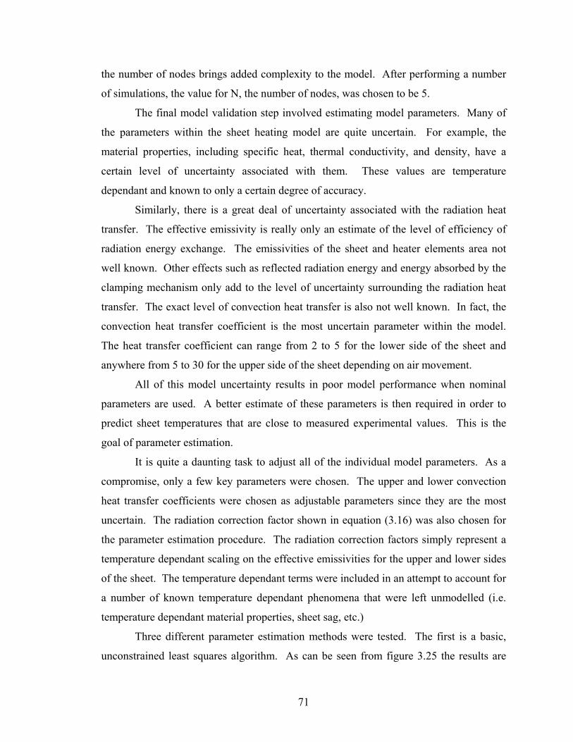
71
the number of nodes brings added complexity to the model. After performing a number
of simulations, the value for N, the number of nodes, was chosen to be 5.
The final model validation step involved estimating model parameters. Many of
the parameters within the sheet heating model are quite uncertain. For example, the
material properties, including specific heat, thermal conductivity, and density, have a
certain level of uncertainty associated with them. These values are temperature
dependant and known to only a certain degree of accuracy.
Similarly, there is a great deal of uncertainty associated with the radiation heat
transfer. The effective emissivity is really only an estimate of the level of efficiency of
radiation energy exchange. The emissivities of the sheet and heater elements area not
well known. Other effects such as reflected radiation energy and energy absorbed by the
clamping mechanism only add to the level of uncertainty surrounding the radiation heat
transfer. The exact level of convection heat transfer is also not well known. In fact, the
convection heat transfer coefficient is the most uncertain parameter within the model.
The heat transfer coefficient can range from 2 to 5 for the lower side of the sheet and
anywhere from 5 to 30 for the upper side of the sheet depending on air movement.
All of this model uncertainty results in poor model performance when nominal
parameters are used. A better estimate of these parameters is then required in order to
predict sheet temperatures that are close to measured experimental values. This is the
goal of parameter estimation.
It is quite a daunting task to adjust all of the individual model parameters. As a
compromise, only a few key parameters were chosen. The upper and lower convection
heat transfer coefficients were chosen as adjustable parameters since they are the most
uncertain. The radiation correction factor shown in equation (3.16) was also chosen for
the parameter estimation procedure. The radiation correction factors simply represent a
temperature dependant scaling on the effective emissivities for the upper and lower sides
of the sheet. The temperature dependant terms were included in an attempt to account for
a number of known temperature dependant phenomena that were left unmodelled (i.e.
temperature dependant material properties, sheet sag, etc.)
Three different parameter estimation methods were tested. The first is a basic,
unconstrained least squares algorithm. As can be seen from figure 3.25 the results are
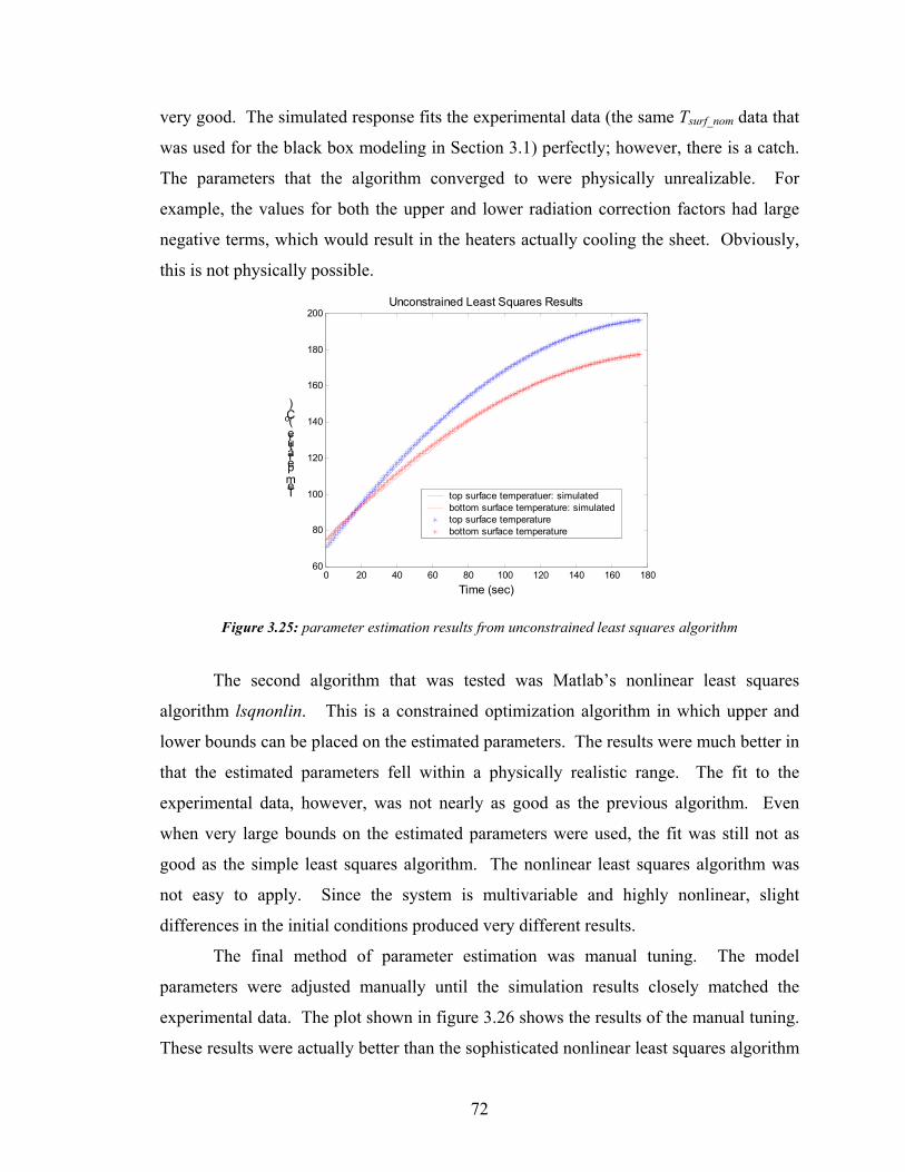
72
very good. The simulated response fits the experimental data (the same Tsurf_nom data that
was used for the black box modeling in Section 3.1) perfectly; however, there is a catch.
The parameters that the algorithm converged to were physically unrealizable. For
example, the values for both the upper and lower radiation correction factors had large
negative terms, which would result in the heaters actually cooling the sheet. Obviously,
this is not physically possible.
0 20 40 60 80 100 120 140 160 18060
80
100
120
140
160
180
200
Time (sec)
Temperature (
oC)
Unconstrained Least Squares Results
top surface temperatuer: simulated bottom surface temperature: simulatedtop surface temperature bottom surface temperature
Figure 3.25: parameter estimation results from unconstrained least squares algorithm
The second algorithm that was tested was Matlab’s nonlinear least squares
algorithm lsqnonlin. This is a constrained optimization algorithm in which upper and
lower bounds can be placed on the estimated parameters. The results were much better in
that the estimated parameters fell within a physically realistic range. The fit to the
experimental data, however, was not nearly as good as the previous algorithm. Even
when very large bounds on the estimated parameters were used, the fit was still not as
good as the simple least squares algorithm. The nonlinear least squares algorithm was
not easy to apply. Since the system is multivariable and highly nonlinear, slight
differences in the initial conditions produced very different results.
The final method of parameter estimation was manual tuning. The model
parameters were adjusted manually until the simulation results closely matched the
experimental data. The plot shown in figure 3.26 shows the results of the manual tuning.
These results were actually better than the sophisticated nonlinear least squares algorithm
73
results. Also, the time required to perform the manual tuning was not significant. Only a
few adjustments had to be made before the results shown were obtained. The final
estimated parameters can be found in the Matlab code given in the Appendix. The fact
that the radiation correction factors were quite large suggests that the initial estimates of
the effective emissivities were way off. This may not necessarily be the case. It is
believed that the large correction factors are a result of the discretization of the system.
Parameter estimation of this scale is not a trivial process. New techniques and/or
“correction functions” could easily be the subject of future work. Additional parameter
estimation and model validation results will be given in [26].
3.4.2.3 Disturbances
Sheet heating is subject to a number of disturbances. The most notable is air
movement in and around the oven. As mentioned earlier, airflow over the sheet surface
can have a drastic effect on the convection heat transfer coefficient. The other important
disturbance acting on the system is machine drift. The machine operating parameters can
change significantly with time. These changes subsequently result in alterations to the
sheet heating dynamics. Due to time constraints, the stochastic properties of the process
were not studied in detail. This will be the subject of future work most likely related to
cycle-to-cycle control design.
0 20 40 60 80 100 120 140 160 18060
80
100
120
140
160
180
200Manual Tuning Parameter Estimation Results
Time (s)
Temperature (
oC)
top surface: simulated bottom surface: simulatedtop surface bottom surface
Figure 3.26: manual tuning parameter estimation results
74
3.4.2.4 Future Modeling Improvements
Due to the originality of this project, the modeling work on sheet heating
presented in this report was only a first attempt. A number of improvements are possible.
To begin, a database of temperature dependent material properties is necessary. Some
thermoplastic materials exhibit highly nonlinear, temperature dependent behavior
characterized by varying specific heat, density, and emissivity values. Using temperature
dependent material properties in the sheet heating model will greatly improve
performance.
Performance can also be significantly improved by using time-varying values for
sheet thickness and radiation view factors, which would better account for the effects of
sheet sag. These values would need to be found using the IMI thermoforming simulation
software. At the time of completion of this project, the time-varying radiation view
factors could not be extracted from the simulation software. A few minor programming
modifications were required first.
Finally, improvements could be made by studying some of the unmodelled
dynamics including the effects from reflected radiation within the oven and volumetric
absorption of radiation energy by the sheet. Proper examination of these topics would,
however, require expert knowledge of thermal radiation heat transfer.
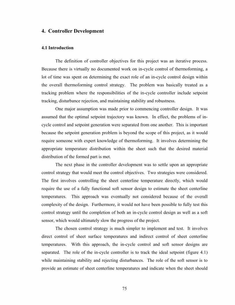
75
4. Controller Development
4.1 Introduction
The definition of controller objectives for this project was an iterative process.
Because there is virtually no documented work on in-cycle control of thermoforming, a
lot of time was spent on determining the exact role of an in-cycle control design within
the overall thermoforming control strategy. The problem was basically treated as a
tracking problem where the responsibilities of the in-cycle controller include setpoint
tracking, disturbance rejection, and maintaining stability and robustness.
One major assumption was made prior to commencing controller design. It was
assumed that the optimal setpoint trajectory was known. In effect, the problems of in-
cycle control and setpoint generation were separated from one another. This is important
because the setpoint generation problem is beyond the scope of this project, as it would
require someone with expert knowledge of thermoforming. It involves determining the
appropriate temperature distribution within the sheet such that the desired material
distribution of the formed part is met.
The next phase in the controller development was to settle upon an appropriate
control strategy that would meet the control objectives. Two strategies were considered.
The first involves controlling the sheet centerline temperature directly, which would
require the use of a fully functional soft sensor design to estimate the sheet centerline
temperatures. This approach was eventually not considered because of the overall
complexity of the design. Furthermore, it would not have been possible to fully test this
control strategy until the completion of both an in-cycle control design as well as a soft
sensor, which would ultimately slow the progress of the project.
The chosen control strategy is much simpler to implement and test. It involves
direct control of sheet surface temperatures and indirect control of sheet centerline
temperatures. With this approach, the in-cycle control and soft sensor designs are
separated. The role of the in-cycle controller is to track the ideal setpoint (figure 4.1)
while maintaining stability and rejecting disturbances. The role of the soft sensor is to
provide an estimate of sheet centerline temperatures and indicate when the sheet should
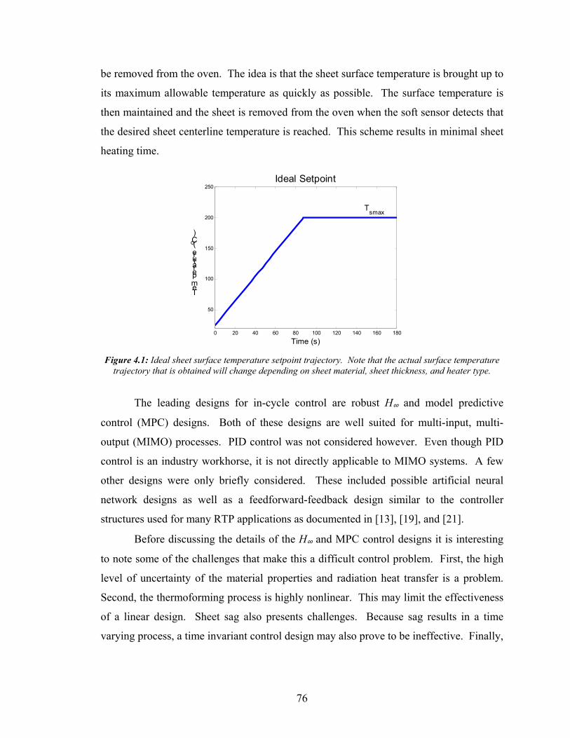
76
be removed from the oven. The idea is that the sheet surface temperature is brought up to
its maximum allowable temperature as quickly as possible. The surface temperature is
then maintained and the sheet is removed from the oven when the soft sensor detects that
the desired sheet centerline temperature is reached. This scheme results in minimal sheet
heating time.
0 20 40 60 80 100 120 140 160 180
50
100
150
200
250
Time (s)
Temperature (
oC)
Ideal Setpoint
Tsmax
Figure 4.1: Ideal sheet surface temperature setpoint trajectory. Note that the actual surface temperature
trajectory that is obtained will change depending on sheet material, sheet thickness, and heater type.
The leading designs for in-cycle control are robust H∞ and model predictive
control (MPC) designs. Both of these designs are well suited for multi-input, multi-
output (MIMO) processes. PID control was not considered however. Even though PID
control is an industry workhorse, it is not directly applicable to MIMO systems. A few
other designs were only briefly considered. These included possible artificial neural
network designs as well as a feedforward-feedback design similar to the controller
structures used for many RTP applications as documented in [13], [19], and [21].
Before discussing the details of the H∞ and MPC control designs it is interesting
to note some of the challenges that make this a difficult control problem. First, the high
level of uncertainty of the material properties and radiation heat transfer is a problem.
Second, the thermoforming process is highly nonlinear. This may limit the effectiveness
of a linear design. Sheet sag also presents challenges. Because sag results in a time
varying process, a time invariant control design may also prove to be ineffective. Finally,
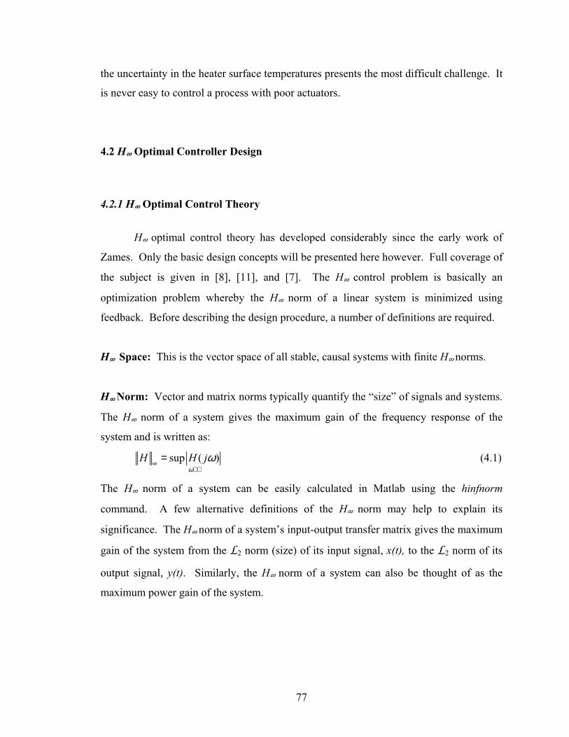
77
the uncertainty in the heater surface temperatures presents the most difficult challenge. It
is never easy to control a process with poor actuators.
4.2 H∞ Optimal Controller Design
4.2.1 H∞ Optimal Control Theory
H∞ optimal control theory has developed considerably since the early work of
Zames. Only the basic design concepts will be presented here however. Full coverage of
the subject is given in [8], [11], and [7]. The H∞ control problem is basically an
optimization problem whereby the H∞ norm of a linear system is minimized using
feedback. Before describing the design procedure, a number of definitions are required.
H∞ Space: This is the vector space of all stable, causal systems with finite H∞ norms.
H∞ Norm: Vector and matrix norms typically quantify the “size” of signals and systems.
The H∞ norm of a system gives the maximum gain of the frequency response of the
system and is written as:
sup ( )H H jω
ω∞
∈ℜ= (4.1)
The H∞ norm of a system can be easily calculated in Matlab using the hinfnorm
command. A few alternative definitions of the H∞ norm may help to explain its
significance. The H∞ norm of a system’s input-output transfer matrix gives the maximum
gain of the system from the L2 norm (size) of its input signal, x(t), to the L2 norm of its
output signal, y(t). Similarly, the H∞ norm of a system can also be thought of as the
maximum power gain of the system.
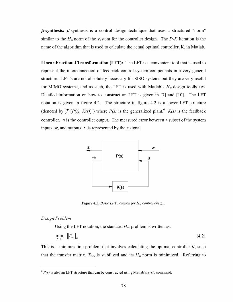
78
µ-synthesis: µ-synthesis is a control design technique that uses a structured "norm"
similar to the H∞ norm of the system for the controller design. The D-K Iteration is the
name of the algorithm that is used to calculate the actual optimal controller, K, in Matlab.
Linear Fractional Transformation (LFT): The LFT is a convenient tool that is used to
represent the interconnection of feedback control system components in a very general
structure. LFT’s are not absolutely necessary for SISO systems but they are very useful
for MIMO systems, and as such, the LFT is used with Matlab’s H∞ design toolboxes.
Detailed information on how to construct an LFT is given in [7] and [10]. The LFT
notation is given in figure 4.2. The structure in figure 4.2 is a lower LFT structure
(denoted by FL[P(s), K(s)] ) where P(s) is the generalized plant.6 K(s) is the feedback
controller. u is the controller output. The measured error between a subset of the system
inputs, w, and outputs, z, is represented by the e signal.
K(s)
P(s)
z w
u-e
Figure 4.2: Basic LFT notation for H∞ control design.
Design Problem
Using the LFT notation, the standard H∞ problem is written as:
min zwK ST
∞∈ (4.2)
This is a minimization problem that involves calculating the optimal controller K, such
that the transfer matrix, Tzw, is stabilized and its H∞ norm is minimized. Referring to
6 P(s) is also an LFT structure that can be constructed using Matlab’s sysic command.
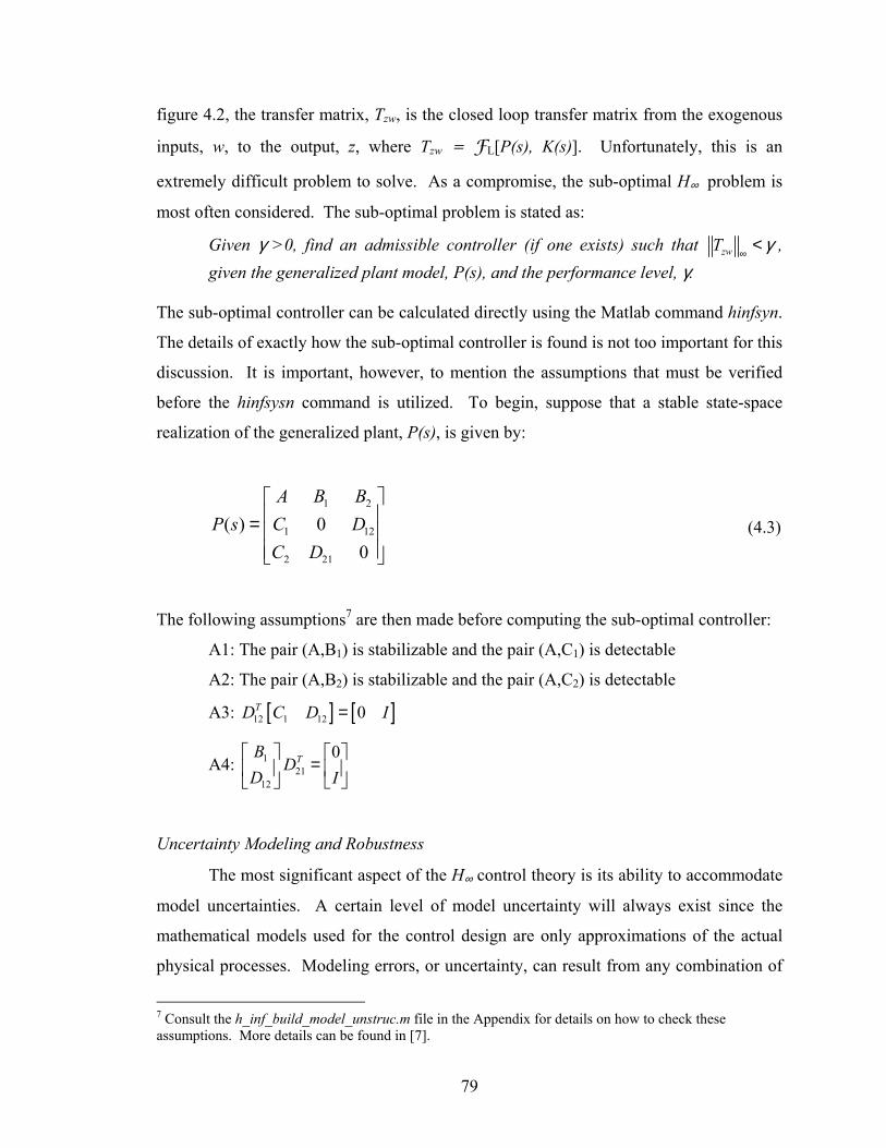
79
figure 4.2, the transfer matrix, Tzw, is the closed loop transfer matrix from the exogenous
inputs, w, to the output, z, where Tzw = FL[P(s), K(s)]. Unfortunately, this is an
extremely difficult problem to solve. As a compromise, the sub-optimal H∞ problem is
most often considered. The sub-optimal problem is stated as:
Given γ >0, find an admissible controller (if one exists) such that zwT γ∞
< , given the generalized plant model, P(s), and the performance level, γ.
The sub-optimal controller can be calculated directly using the Matlab command hinfsyn.
The details of exactly how the sub-optimal controller is found is not too important for this
discussion. It is important, however, to mention the assumptions that must be verified
before the hinfsysn command is utilized. To begin, suppose that a stable state-space
realization of the generalized plant, P(s), is given by:
1 2
1 12
2 21
( ) 00
A B BP s C D
C D
=
(4.3)
The following assumptions7 are then made before computing the sub-optimal controller:
A1: The pair (A,B1) is stabilizable and the pair (A,C1) is detectable
A2: The pair (A,B2) is stabilizable and the pair (A,C2) is detectable
A3: [ ] [ ]12 1 12 0TD C D I=
A4: 121
12
0TBD
D I
=
Uncertainty Modeling and Robustness
The most significant aspect of the H∞ control theory is its ability to accommodate
model uncertainties. A certain level of model uncertainty will always exist since the
mathematical models used for the control design are only approximations of the actual
physical processes. Modeling errors, or uncertainty, can result from any combination of
7 Consult the h_inf_build_model_unstruc.m file in the Appendix for details on how to check these assumptions. More details can be found in [7].
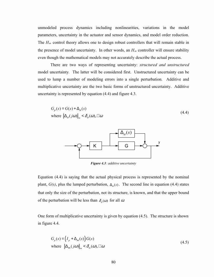
80
unmodeled process dynamics including nonlinearities, variations in the model
parameters, uncertainty in the actuator and sensor dynamics, and model order reduction.
The H∞ control theory allows one to design robust controllers that will remain stable in
the presence of model uncertainty. In other words, an H∞ controller will ensure stability
even though the mathematical models may not accurately describe the actual process.
There are two ways of representing uncertainty: structured and unstructured
model uncertainty. The latter will be considered first. Unstructured uncertainty can be
used to lump a number of modeling errors into a single perturbation. Additive and
multiplicative uncertainty are the two basic forms of unstructured uncertainty. Additive
uncertainty is represented by equation (4.4) and figure 4.3.
( ) ( ) ( )
where ( ) ( ),p a
a a
G s G s s
jω δ ω ω∞
= + ∆
∆ < ∀ (4.4)
yGK
Figure 4.3: additive uncertainty
Equation (4.4) is saying that the actual physical process is represented by the nominal
plant, G(s), plus the lumped perturbation, ( )a s∆ . The second line in equation (4.4) states
that only the size of the perturbation, not its structure, is known, and that the upper bound
of the perturbation will be less than ( )aδ ω for all ω.
One form of multiplicative uncertainty is given by equation (4.5). The structure is shown
in figure 4.4.
( )
m
( ) ( ) ( )
where ( ) ( ),p p
m
mG s I s G s
jω δ ω ω∞
= + ∆
∆ < ∀ (4.5)
( )a s∆
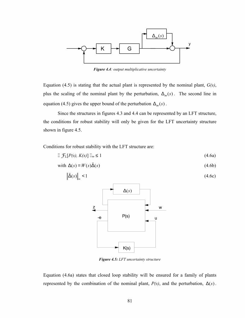
81
yGK
Figure 4.4: output multiplicative uncertainty
Equation (4.5) is stating that the actual plant is represented by the nominal plant, G(s),
plus the scaling of the nominal plant by the perturbation, ( )m s∆ . The second line in
equation (4.5) gives the upper bound of the perturbation ( )m s∆ .
Since the structures in figures 4.3 and 4.4 can be represented by an LFT structure,
the conditions for robust stability will only be given for the LFT uncertainty structure
shown in figure 4.5.
Conditions for robust stability with the LFT structure are:
FL[P(s), K(s)] ∞ ≤ 1 (4.6a)
with ( ) ( ) ( )s W s s∆ = ∆ (4.6b)
( ) 1s∞
∆ < (4.6c)
K(s)
P(s)
z w
u-e
Figure 4.5: LFT uncertainty structure
Equation (4.6a) states that closed loop stability will be ensured for a family of plants
represented by the combination of the nominal plant, P(s), and the perturbation, ( )s∆ .
( )m s∆
( )s∆
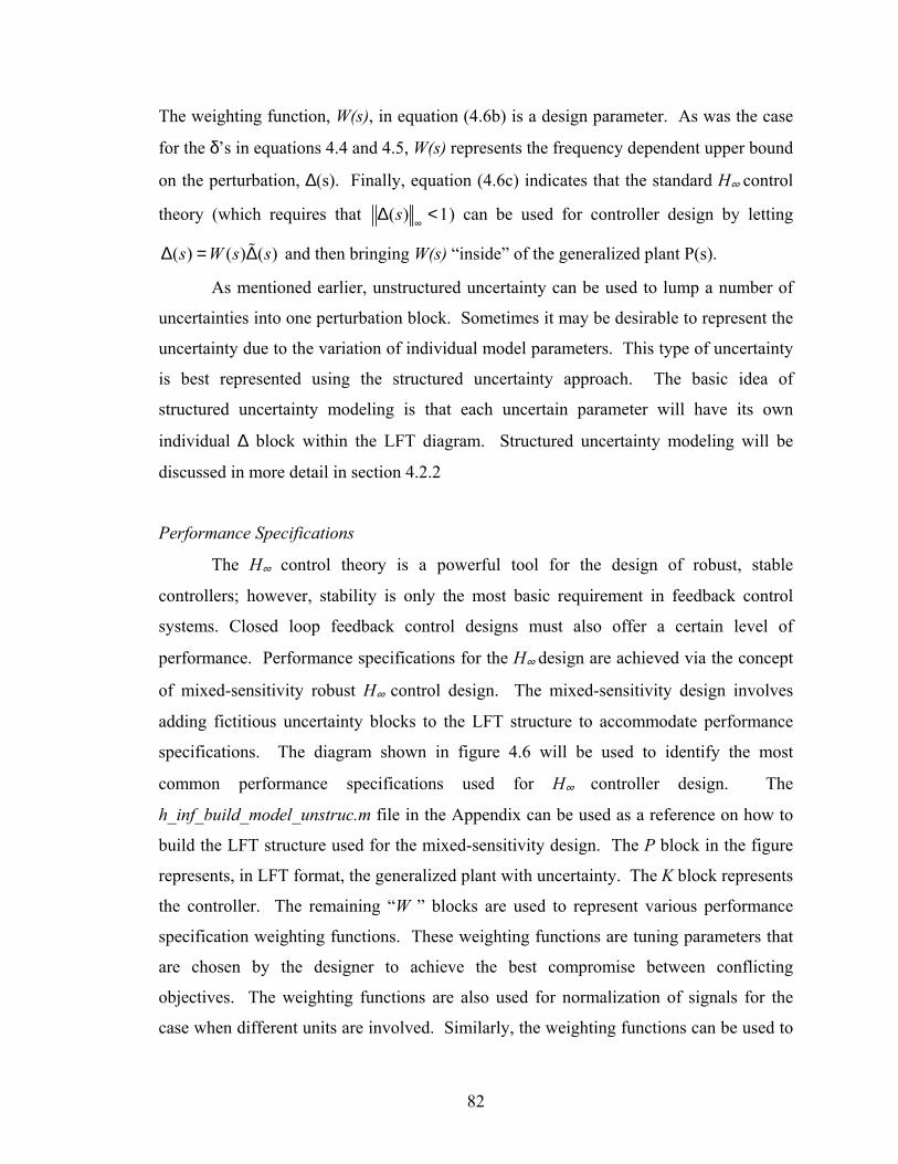
82
The weighting function, W(s), in equation (4.6b) is a design parameter. As was the case
for the δ’s in equations 4.4 and 4.5, W(s) represents the frequency dependent upper bound
on the perturbation, ∆(s). Finally, equation (4.6c) indicates that the standard H∞ control
theory (which requires that ( ) 1s∞
∆ < ) can be used for controller design by letting
( ) ( ) ( )s W s s∆ = ∆ and then bringing W(s) “inside” of the generalized plant P(s).
As mentioned earlier, unstructured uncertainty can be used to lump a number of
uncertainties into one perturbation block. Sometimes it may be desirable to represent the
uncertainty due to the variation of individual model parameters. This type of uncertainty
is best represented using the structured uncertainty approach. The basic idea of
structured uncertainty modeling is that each uncertain parameter will have its own
individual ∆ block within the LFT diagram. Structured uncertainty modeling will be
discussed in more detail in section 4.2.2
Performance Specifications
The H∞ control theory is a powerful tool for the design of robust, stable
controllers; however, stability is only the most basic requirement in feedback control
systems. Closed loop feedback control designs must also offer a certain level of
performance. Performance specifications for the H∞ design are achieved via the concept
of mixed-sensitivity robust H∞ control design. The mixed-sensitivity design involves
adding fictitious uncertainty blocks to the LFT structure to accommodate performance
specifications. The diagram shown in figure 4.6 will be used to identify the most
common performance specifications used for H∞ controller design. The
h_inf_build_model_unstruc.m file in the Appendix can be used as a reference on how to
build the LFT structure used for the mixed-sensitivity design. The P block in the figure
represents, in LFT format, the generalized plant with uncertainty. The K block represents
the controller. The remaining “W ” blocks are used to represent various performance
specification weighting functions. These weighting functions are tuning parameters that
are chosen by the designer to achieve the best compromise between conflicting
objectives. The weighting functions are also used for normalization of signals for the
case when different units are involved. Similarly, the weighting functions can be used to
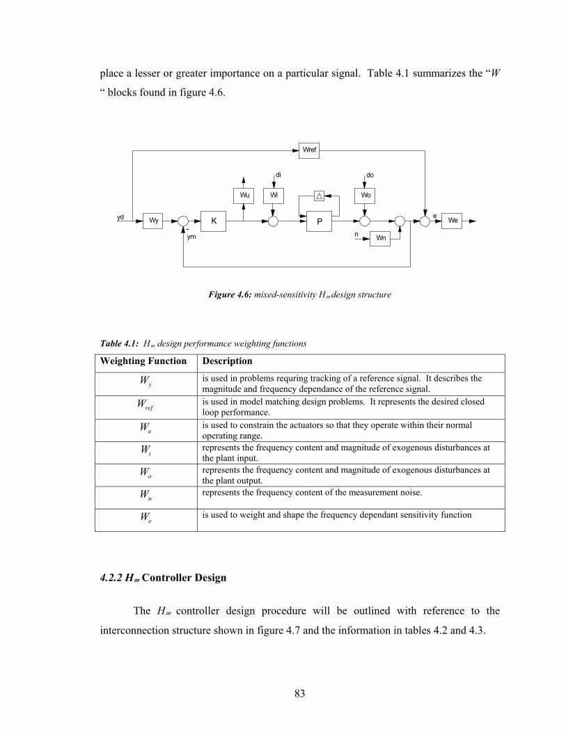
83
place a lesser or greater importance on a particular signal. Table 4.1 summarizes the “W
“ blocks found in figure 4.6.
Wu Wi Wo
Wy
Wref
K P
di
yd
Wn
We
n-ym
e
do
Figure 4.6: mixed-sensitivity H∞ design structure
Table 4.1: H∞ design performance weighting functions
Weighting Function Description
yW is used in problems requring tracking of a reference signal. It describes the magnitude and frequency dependance of the reference signal.
refW is used in model matching design problems. It represents the desired closed loop performance.
uW is used to constrain the actuators so that they operate within their normal operating range.
iW represents the frequency content and magnitude of exogenous disturbances at the plant input.
oW represents the frequency content and magnitude of exogenous disturbances at the plant output.
nW represents the frequency content of the measurement noise.
eW is used to weight and shape the frequency dependant sensitivity function
4.2.2 H∞ Controller Design
The H∞ controller design procedure will be outlined with reference to the
interconnection structure shown in figure 4.7 and the information in tables 4.2 and 4.3.

84
Wu
Wy
Wre
f
KP
yd
Wn
We
n
- ym
H
Wh
WpF
Wf
Tair
euc
u
ydes
Figure 4.7: H∞ controller design interconnection
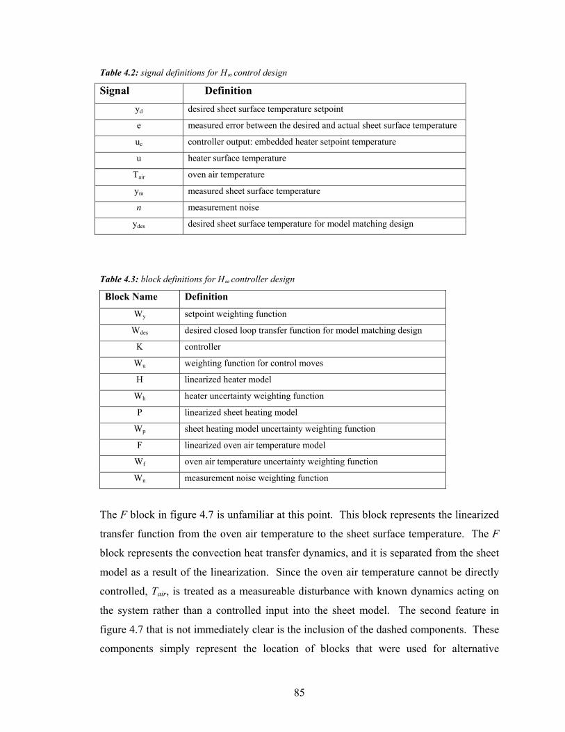
85
Table 4.2: signal definitions for H∞ control design
Signal Definition yd desired sheet surface temperature setpoint
e measured error between the desired and actual sheet surface temperature
uc controller output: embedded heater setpoint temperature
u heater surface temperature
Tair oven air temperature
ym measured sheet surface temperature
n measurement noise
ydes desired sheet surface temperature for model matching design
Table 4.3: block definitions for H∞ controller design
Block Name Definition
Wy setpoint weighting function
Wdes desired closed loop transfer function for model matching design
K controller
Wu weighting function for control moves
H linearized heater model
Wh heater uncertainty weighting function
P linearized sheet heating model
Wp sheet heating model uncertainty weighting function
F linearized oven air temperature model
Wf oven air temperature uncertainty weighting function
Wn measurement noise weighting function
The F block in figure 4.7 is unfamiliar at this point. This block represents the linearized
transfer function from the oven air temperature to the sheet surface temperature. The F
block represents the convection heat transfer dynamics, and it is separated from the sheet
model as a result of the linearization. Since the oven air temperature cannot be directly
controlled, Tair, is treated as a measureable disturbance with known dynamics acting on
the system rather than a controlled input into the sheet model. The second feature in
figure 4.7 that is not immediately clear is the inclusion of the dashed components. These
components simply represent the location of blocks that were used for alternative
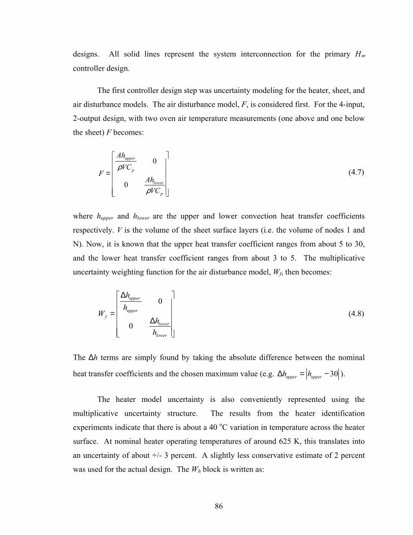
86
designs. All solid lines represent the system interconnection for the primary H∞
controller design.
The first controller design step was uncertainty modeling for the heater, sheet, and
air disturbance models. The air disturbance model, F, is considered first. For the 4-input,
2-output design, with two oven air temperature measurements (one above and one below
the sheet) F becomes:
0
0
upper
p
lower
p
AhVC
FAh
VC
ρ
ρ
=
(4.7)
where hupper and hlower are the upper and lower convection heat transfer coefficients
respectively. V is the volume of the sheet surface layers (i.e. the volume of nodes 1 and
N). Now, it is known that the upper heat transfer coefficient ranges from about 5 to 30,
and the lower heat transfer coefficient ranges from about 3 to 5. The multiplicative
uncertainty weighting function for the air disturbance model, Wf, then becomes:
0
0
upper
upperf
lower
lower
hh
Wh
h
∆ = ∆
(4.8)
The ∆h terms are simply found by taking the absolute difference between the nominal
heat transfer coefficients and the chosen maximum value (e.g. 30upper upperh h∆ = − ).
The heater model uncertainty is also conveniently represented using the
multiplicative uncertainty structure. The results from the heater identification
experiments indicate that there is about a 40 oC variation in temperature across the heater
surface. At nominal heater operating temperatures of around 625 K, this translates into
an uncertainty of about +/- 3 percent. A slightly less conservative estimate of 2 percent
was used for the actual design. The Wh block is written as:
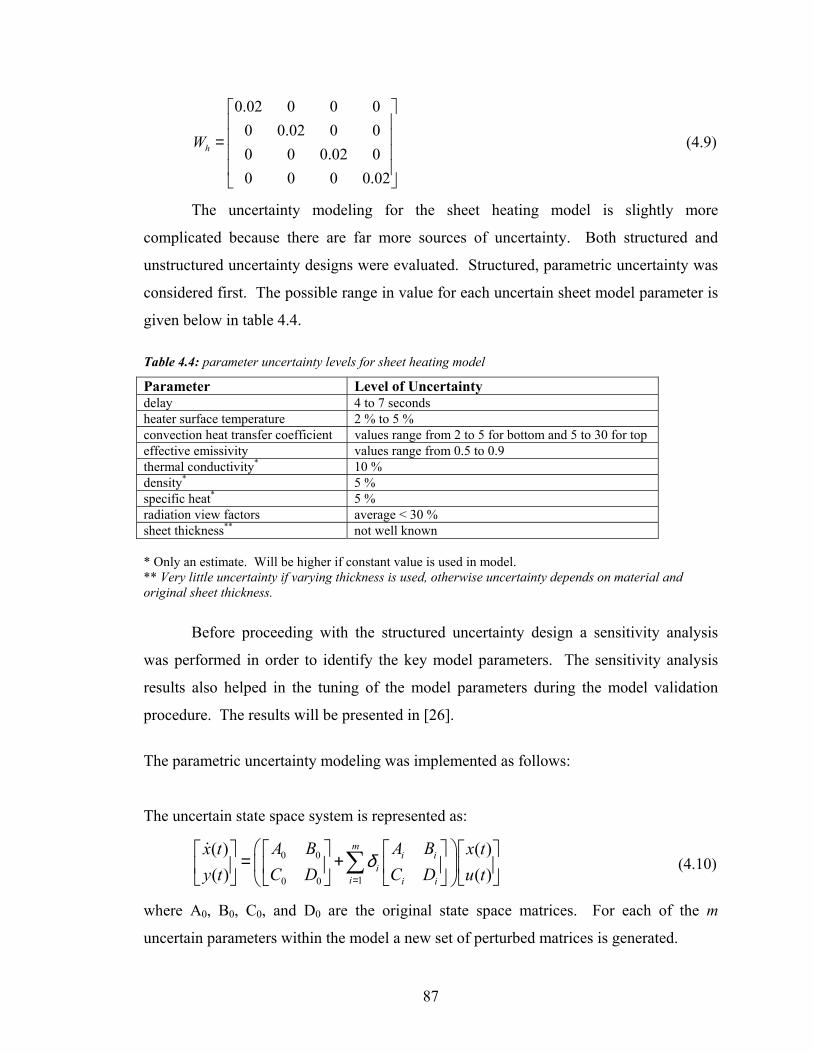
87
0.02 0 0 00 0.02 0 00 0 0.02 00 0 0 0.02
hW
=
(4.9)
The uncertainty modeling for the sheet heating model is slightly more
complicated because there are far more sources of uncertainty. Both structured and
unstructured uncertainty designs were evaluated. Structured, parametric uncertainty was
considered first. The possible range in value for each uncertain sheet model parameter is
given below in table 4.4.
Table 4.4: parameter uncertainty levels for sheet heating model
Parameter Level of Uncertainty delay 4 to 7 seconds heater surface temperature 2 % to 5 % convection heat transfer coefficient values range from 2 to 5 for bottom and 5 to 30 for top effective emissivity values range from 0.5 to 0.9 thermal conductivity* 10 % density* 5 % specific heat* 5 % radiation view factors average < 30 % sheet thickness** not well known * Only an estimate. Will be higher if constant value is used in model. ** Very little uncertainty if varying thickness is used, otherwise uncertainty depends on material and original sheet thickness.
Before proceeding with the structured uncertainty design a sensitivity analysis
was performed in order to identify the key model parameters. The sensitivity analysis
results also helped in the tuning of the model parameters during the model validation
procedure. The results will be presented in [26].
The parametric uncertainty modeling was implemented as follows:
The uncertain state space system is represented as:
0 0
10 0
( ) ( )( ) ( )
mi i
ii i i
A B A Bx t x tC D C Dy t u t
δ=
= +
∑ (4.10)
where A0, B0, C0, and D0 are the original state space matrices. For each of the m
uncertain parameters within the model a new set of perturbed matrices is generated.
88
now let i ii
i i
A Br rank
C D
=
(4.11)
and then factor each matrix using singular value decomposition as:
[ ]i i ii i
i i i
A B EG H
C D F
=
(4.12)
where [ ]i i( ) ( ) , G Hi ii
i
n ny r r n nyER R
F+ × × +
∈ ∈
Now define a new generalized plant with the added inputs and outputs:
0 0 1
0 0 1
1 1 1 10 0
0 0
m
m
m m m m
x A B E E xy C D F F uz G H w
z G G w
=
(4.13)
The h_inf_build_model_struc.m file in the Appendix can be consulted for more details on
the parametric uncertainty modeling procedure.
An unstructured output multiplicative uncertainty modeling approach was also
considered. The results shown in figure 4.8 were obtained by performing a Monte Carlo
type analysis, which involved comparing the frequency response of various perturbed
models with a nominal response. As can be seen from the figure, the level of uncertainty
is very high even at low frequencies, where the uncertainty is nearly 125 percent.
Fortunately, the bandwidth of the system is very low (aprox. 0.001 rads/sec for the sheet
heating model), which means that the very high uncertainty at higher frequencies can be
ignored.
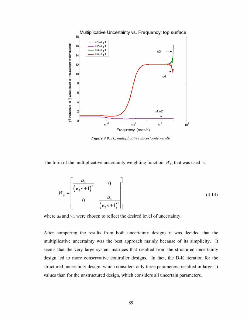
89
10-2 100 102 1040
2
4
6
8
10
12
14
16
18
Frequency (rads/s)
% change in magnitude of frequency response
Multiplicative Uncertainty vs. Frequency: top surface
u1-->y1u2-->y1u3-->y1u4-->y1
u3
u4
u1,u2
Figure 4.8: H∞ multiplicative uncertainty results
The form of the multiplicative uncertainty weighting function, Wp, that was used is:
( )
( )
02
02
01
01
bp
b
aw s
Wa
w s
+ =
+
(4.14)
where a0 and wb were chosen to reflect the desired level of uncertainty.
After comparing the results from both uncertainty designs it was decided that the
multiplicative uncertainty was the best approach mainly because of its simplicity. It
seems that the very large system matrices that resulted from the structured uncertainty
design led to more conservative controller designs. In fact, the D-K iteration for the
structured uncertainty design, which considers only three parameters, resulted in larger µ
values than for the unstructured design, which considers all uncertain parameters.
90
Performance Specifications
The performance specifications will now be discussed with reference to the
design structure from figure 4.7.
Measurement Noise
Measurement noise is not a major concern for the Raytek IR sensors used on the
IMI machine because the measurements are pre-filtered and quite stable. A low weighted
Wn was chosen as:
1 5 0
0 1 5n
eW
e−
= − (4.15)
Setpoint
A weighting function on the setpoint reference signal was used for some designs
to account for the fact that the reference signal, yd, will never contain any high frequency
content. The use of Wy allowed for a more aggressive weighting on the error function We.
Wy was chosen as:
1 0500 1
10500 1
ysW
s
+= +
(4.16)
Model Matching Design
The model matching design shown in figure 4.7 was used in an attempt to “slow”
the control action and reduce some of the overshoot that was observed in some of the
early simulations. The form for Wdes is that of a 2nd order transfer function:
91
2
2 2
2
2 2
02
02
n
n ndes
n
n n
s sW
s s
ωζω ω
ωζω ω
+ + =
+ +
(4.17)
Values for ωn were chosen to be around 0.001 and the damping ratio, ζ, was chosen to be
around 0.8.
Control Moves
The control moves were constrained with the use of Wu. The desired shape of this
weighting function is shown below in figure 4.9. The larger weighting at higher
frequencies is used to prevent the actuators from responding to any higher frequency
content in the error signal; therefore, Wu constrains the heaters to operate within their
natural bandwidth (aprox. 0.05 rads/sec). This prevents unnecessary wear and tear on the
actuators.
The form of Wu is:
50000 1 0 0 010
50000 10 0 010
50000 10 0 010
50000 10 0 010
u
sks
sksW
sks
sks
+ +
+ += + + + +
(4.18)
The k term was used to scale the numerator of Wu to prevent heater saturation. Values for
k were anywhere between 0.1 and 0.000 001 depending on the simulation conditions.
Error
The weight on the error signal, We, was the primary controller design parameter.
The ideal shape of the frequency response for We is that of a 1st or 2nd order frequency
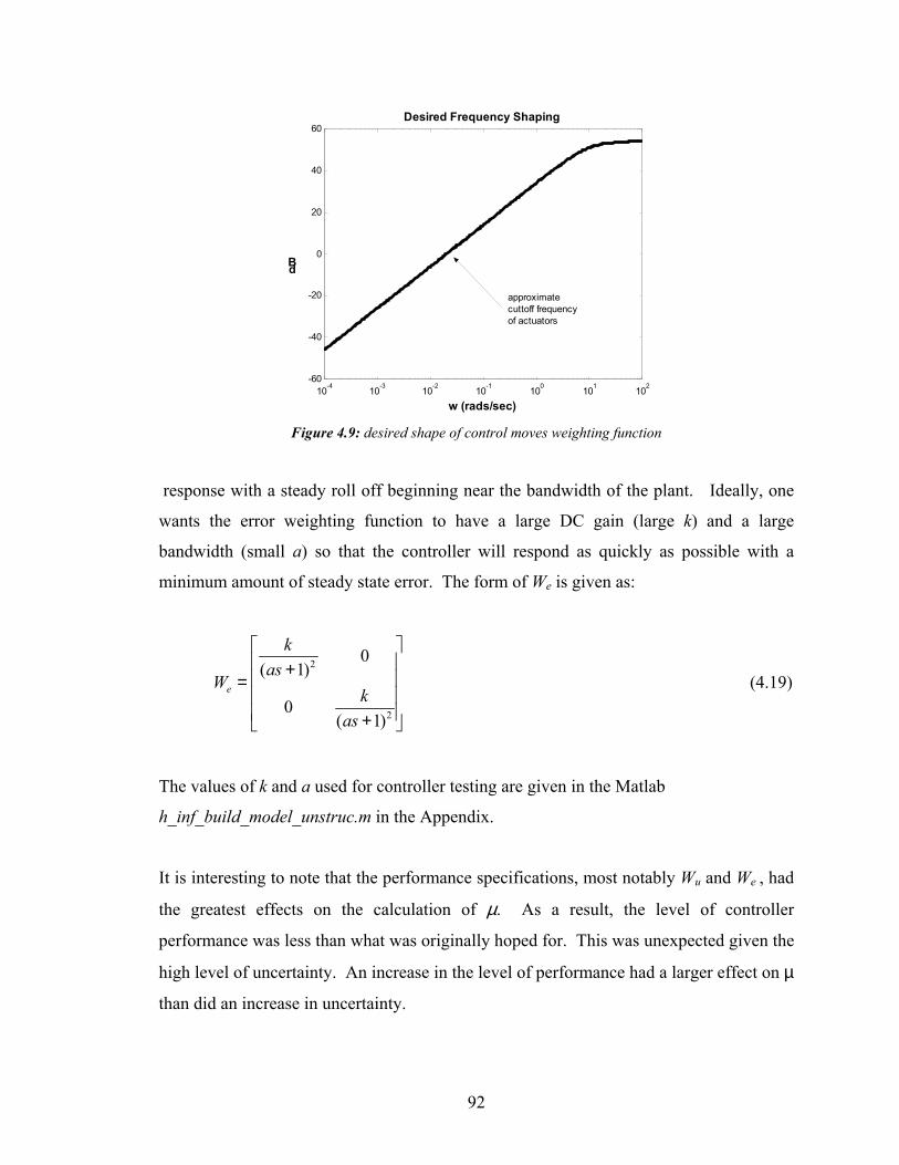
92
10-4 10-3 10-2 10-1 100 101 102-60
-40
-20
0
20
40
60
w (rads/sec)
dB
Desired Frequency Shaping
approximatecuttoff frequencyof actuators
Figure 4.9: desired shape of control moves weighting function
response with a steady roll off beginning near the bandwidth of the plant. Ideally, one
wants the error weighting function to have a large DC gain (large k) and a large
bandwidth (small a) so that the controller will respond as quickly as possible with a
minimum amount of steady state error. The form of We is given as:
2
2
0( 1)
0( 1)
e
kas
Wk
as
+ = +
(4.19)
The values of k and a used for controller testing are given in the Matlab
h_inf_build_model_unstruc.m in the Appendix.
It is interesting to note that the performance specifications, most notably Wu and We , had
the greatest effects on the calculation of µ. As a result, the level of controller
performance was less than what was originally hoped for. This was unexpected given the
high level of uncertainty. An increase in the level of performance had a larger effect on µ
than did an increase in uncertainty.
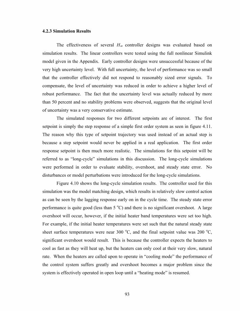
93
4.2.3 Simulation Results
The effectiveness of several H∞ controller designs was evaluated based on
simulation results. The linear controllers were tested using the full nonlinear Simulink
model given in the Appendix. Early controller designs were unsuccessful because of the
very high uncertainty level. With full uncertainty, the level of performance was so small
that the controller effectively did not respond to reasonably sized error signals. To
compensate, the level of uncertainty was reduced in order to achieve a higher level of
robust performance. The fact that the uncertainty level was actually reduced by more
than 50 percent and no stability problems were observed, suggests that the original level
of uncertainty was a very conservative estimate.
The simulated responses for two different setpoints are of interest. The first
setpoint is simply the step response of a simple first order system as seen in figure 4.11.
The reason why this type of setpoint trajectory was used instead of an actual step is
because a step setpoint would never be applied in a real application. The first order
response setpoint is then much more realistic. The simulations for this setpoint will be
referred to as “long-cycle” simulations in this discussion. The long-cycle simulations
were performed in order to evaluate stability, overshoot, and steady state error. No
disturbances or model perturbations were introduced for the long-cycle simulations.
Figure 4.10 shows the long-cycle simulation results. The controller used for this
simulation was the model matching design, which results in relatively slow control action
as can be seen by the lagging response early on in the cycle time. The steady state error
performance is quite good (less than 5 oC) and there is no significant overshoot. A large
overshoot will occur, however, if the initial heater band temperatures were set too high.
For example, if the initial heater temperatures were set such that the natural steady state
sheet surface temperatures were near 300 oC, and the final setpoint value was 200 oC,
significant overshoot would result. This is because the controller expects the heaters to
cool as fast as they will heat up, but the heaters can only cool at their very slow, natural
rate. When the heaters are called upon to operate in “cooling mode” the performance of
the control system suffers greatly and overshoot becomes a major problem since the
system is effectively operated in open loop until a “heating mode” is resumed.
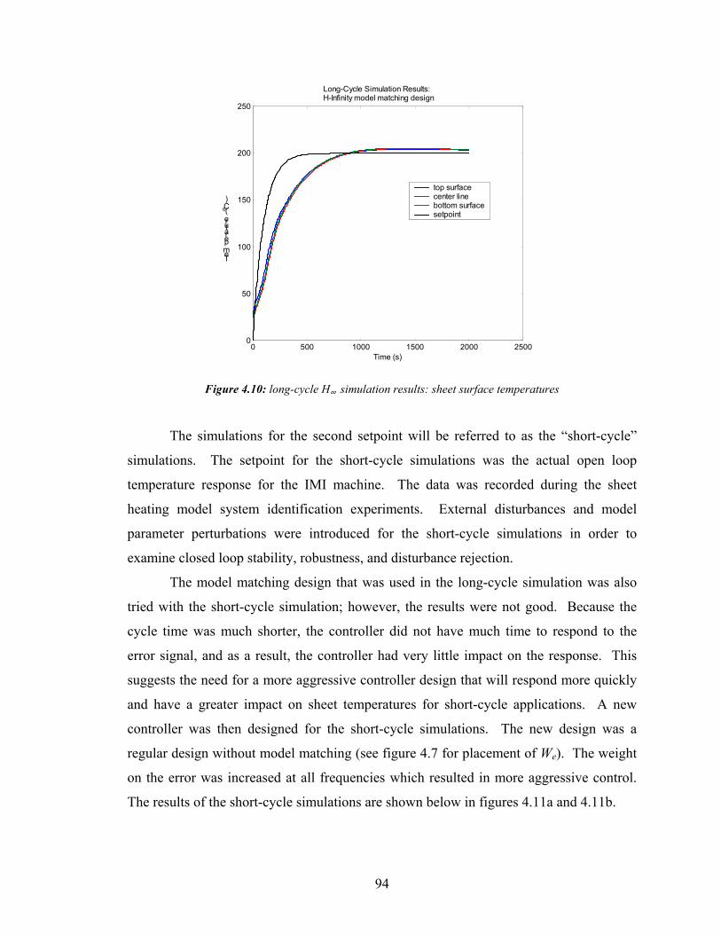
94
0 500 1000 1500 2000 25000
50
100
150
200
250
Long-Cycle Simulation Results: H-Infinity model matching design
Time (s)
Temperature (
oC)
top surface center line bottom surfacesetpoint
Figure 4.10: long-cycle H∞ simulation results: sheet surface temperatures
The simulations for the second setpoint will be referred to as the “short-cycle”
simulations. The setpoint for the short-cycle simulations was the actual open loop
temperature response for the IMI machine. The data was recorded during the sheet
heating model system identification experiments. External disturbances and model
parameter perturbations were introduced for the short-cycle simulations in order to
examine closed loop stability, robustness, and disturbance rejection.
The model matching design that was used in the long-cycle simulation was also
tried with the short-cycle simulation; however, the results were not good. Because the
cycle time was much shorter, the controller did not have much time to respond to the
error signal, and as a result, the controller had very little impact on the response. This
suggests the need for a more aggressive controller design that will respond more quickly
and have a greater impact on sheet temperatures for short-cycle applications. A new
controller was then designed for the short-cycle simulations. The new design was a
regular design without model matching (see figure 4.7 for placement of We). The weight
on the error was increased at all frequencies which resulted in more aggressive control.
The results of the short-cycle simulations are shown below in figures 4.11a and 4.11b.
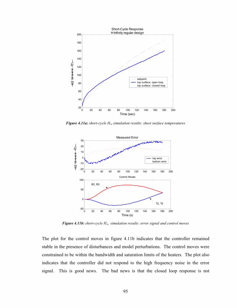
95
0 20 40 60 80 100 120 140 160 180 20020
40
60
80
100
120
140
160
180
200
Time (sec)
Temperature (
oC)
Short-Cycle ResponseH-Infinity regular design
setpoint top surface: open loop top surface: closed loop
Figure 4.11a: short-cycle H∞ simulation results: sheet surface temperatures
0 20 40 60 80 100 120 140 160 180 200-20
-10
0
10
20
30Measured Error
Temperature (
oC)
top error bottom error
0 20 40 60 80 100 120 140 160 180 200-50
0
50
100Control Moves
Time (s)
B2, B5
T2, T5
Figure 4.11b: short-cycle H∞ simulation results: error signal and control moves
The plot for the control moves in figure 4.11b indicates that the controller remained
stable in the presence of disturbances and model perturbations. The control moves were
constrained to be within the bandwidth and saturation limits of the heaters. The plot also
indicates that the controller did not respond to the high frequency noise in the error
signal. This is good news. The bad news is that the closed loop response is not
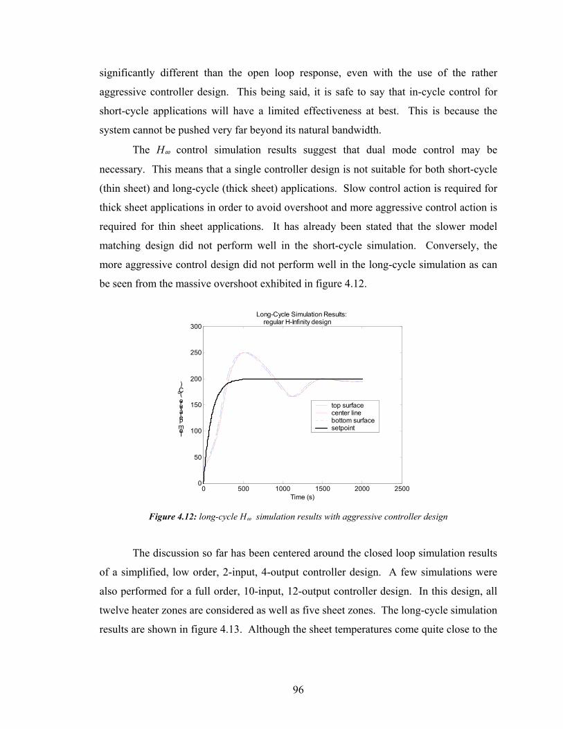
96
significantly different than the open loop response, even with the use of the rather
aggressive controller design. This being said, it is safe to say that in-cycle control for
short-cycle applications will have a limited effectiveness at best. This is because the
system cannot be pushed very far beyond its natural bandwidth.
The H∞ control simulation results suggest that dual mode control may be
necessary. This means that a single controller design is not suitable for both short-cycle
(thin sheet) and long-cycle (thick sheet) applications. Slow control action is required for
thick sheet applications in order to avoid overshoot and more aggressive control action is
required for thin sheet applications. It has already been stated that the slower model
matching design did not perform well in the short-cycle simulation. Conversely, the
more aggressive control design did not perform well in the long-cycle simulation as can
be seen from the massive overshoot exhibited in figure 4.12.
0 500 1000 1500 2000 25000
50
100
150
200
250
300
Long-Cycle Simulation Results:regular H-Infinity design
Time (s)
Temperature (
oC)
top surface center line bottom surfacesetpoint
Figure 4.12: long-cycle H∞ simulation results with aggressive controller design
The discussion so far has been centered around the closed loop simulation results
of a simplified, low order, 2-input, 4-output controller design. A few simulations were
also performed for a full order, 10-input, 12-output controller design. In this design, all
twelve heater zones are considered as well as five sheet zones. The long-cycle simulation
results are shown in figure 4.13. Although the sheet temperatures come quite close to the
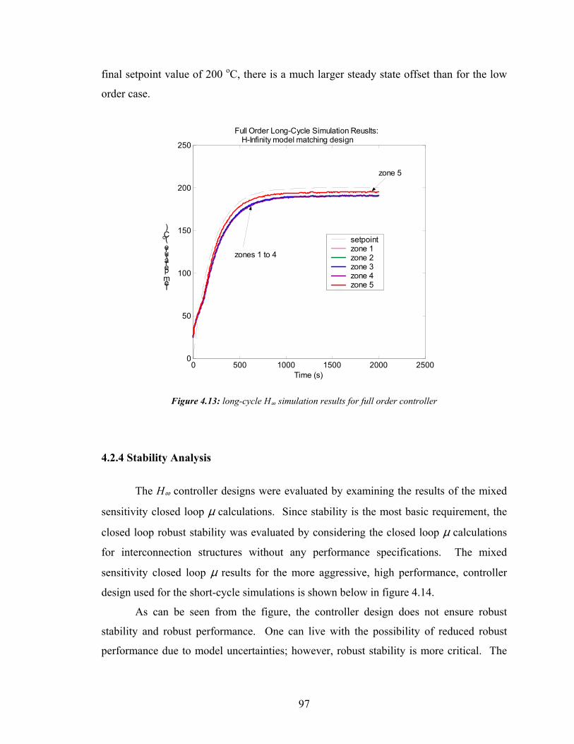
97
final setpoint value of 200 oC, there is a much larger steady state offset than for the low
order case.
0 500 1000 1500 2000 25000
50
100
150
200
250
Full Order Long-Cycle Simulation Reuslts: H-Infinity model matching design
Time (s)
Temperature (
oC)
setpointzone 1 zone 2 zone 3 zone 4 zone 5
zone 5
zones 1 to 4
Figure 4.13: long-cycle H∞ simulation results for full order controller
4.2.4 Stability Analysis
The H∞ controller designs were evaluated by examining the results of the mixed
sensitivity closed loop µ calculations. Since stability is the most basic requirement, the
closed loop robust stability was evaluated by considering the closed loop µ calculations
for interconnection structures without any performance specifications. The mixed
sensitivity closed loop µ results for the more aggressive, high performance, controller
design used for the short-cycle simulations is shown below in figure 4.14.
As can be seen from the figure, the controller design does not ensure robust
stability and robust performance. One can live with the possibility of reduced robust
performance due to model uncertainties; however, robust stability is more critical. The
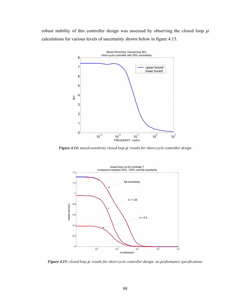
98
robust stability of this controller design was assessed by observing the closed loop µ
calculations for various levels of uncertainty shown below in figure 4.15.
10-3
10-2
10-1
100
101
0
1
2
3
4
5
6
7
8
Mixed Sensitivity Closed-loop MU:short-cycle controller with 50% uncertainty
FREQUENCY (rad/s)
MU
upper boundlower bound
Figure 4.14: mixed-sensitivity closed loop µ results for short-cycle controller design
10-3 10-2 10-1 100 1010
0.2
0.4
0.6
0.8
1
1.2
1.4
w (rads/sec)
closed loop mu
closed loop mu for controller 7comparison between 50%, 125%, and full uncertainty
full uncertainty
k = 1.25
k = 0.5
Figure 4.15: closed loop µ results for short-cycle controller design: no performance specifications
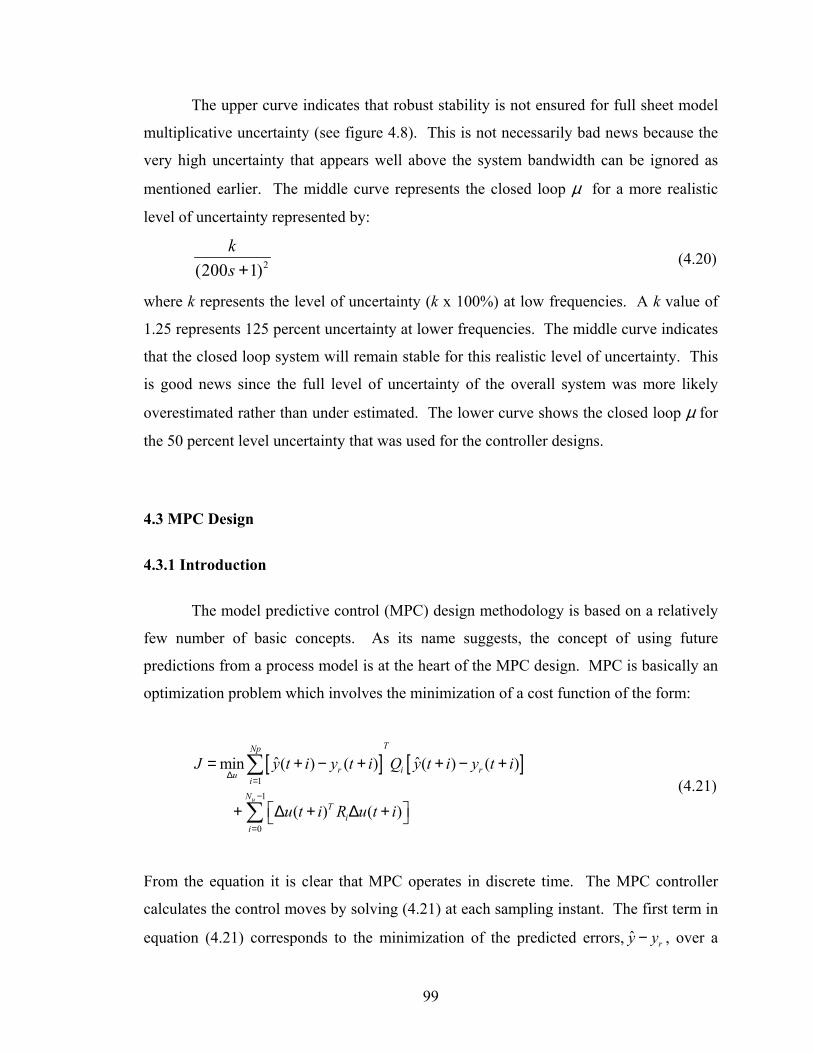
99
The upper curve indicates that robust stability is not ensured for full sheet model
multiplicative uncertainty (see figure 4.8). This is not necessarily bad news because the
very high uncertainty that appears well above the system bandwidth can be ignored as
mentioned earlier. The middle curve represents the closed loop µ for a more realistic
level of uncertainty represented by:
2(200 1)ks +
(4.20)
where k represents the level of uncertainty (k x 100%) at low frequencies. A k value of
1.25 represents 125 percent uncertainty at lower frequencies. The middle curve indicates
that the closed loop system will remain stable for this realistic level of uncertainty. This
is good news since the full level of uncertainty of the overall system was more likely
overestimated rather than under estimated. The lower curve shows the closed loop µ for
the 50 percent level uncertainty that was used for the controller designs.
4.3 MPC Design
4.3.1 Introduction
The model predictive control (MPC) design methodology is based on a relatively
few number of basic concepts. As its name suggests, the concept of using future
predictions from a process model is at the heart of the MPC design. MPC is basically an
optimization problem which involves the minimization of a cost function of the form:
[ ] [ ]
1
1
0
ˆ ˆmin ( ) ( ) ( ) ( )
( ) ( )u
TNp
r i ru i
NT
ii
J y t i y t i Q y t i y t i
u t i R u t i
∆ =
−
=
= + − + + − +
+ ∆ + ∆ +
∑
∑ (4.21)
From the equation it is clear that MPC operates in discrete time. The MPC controller
calculates the control moves by solving (4.21) at each sampling instant. The first term in
equation (4.21) corresponds to the minimization of the predicted errors, ˆ ry y− , over a
100
future time period known as the prediction horizon, Np. The second term in the equation
corresponds to the minimization of the overall size of the control moves, ∆u, over a time
period known as the control horizon, Nu. The Q and R terms are simply scaling terms
that can be used as tuning parameters to shape the weight of the cost function over the
prediction and control horizons respectively.
The general MPC control algorithm involves the following basic steps which are
taken at each sampling instant:
1) sample the process
2) calculate the future outputs, y , over the prediction horizon using the process model
3) calculate the set of control moves over the control horizon by solving the cost function
4) update the process by sending only the first control move (i.e. ∆u(t+0)) to the process, all other future control moves are discarded.
The MPC design methodology actually covers a wide range of controllers; however, they
all follow the same basic algorithm presented above. The primary differences between
designs are the form of the process models that are used to calculate the predicted outputs
and the way in which disturbances are handled. The various MPC designs will not be
discussed here since they are well documented in the literature (see [8]).
4.3.2 MPC Controller Design
Many MPC applications utilize linear models for prediction of future plant
outputs. This can be done if the process is operating in a relatively small region around a
steady state operating point. The use of linear models also greatly simplifies the
minimization of the cost function since the minimization problem can be put into the
form of a standard quadratic programming problem in which a solution is easily
attainable.
Unfortunately, thermoforming does not fall into this category. The process model
is highly nonlinear, and the operating range is wide (25 to 200 oC). As such, it is not
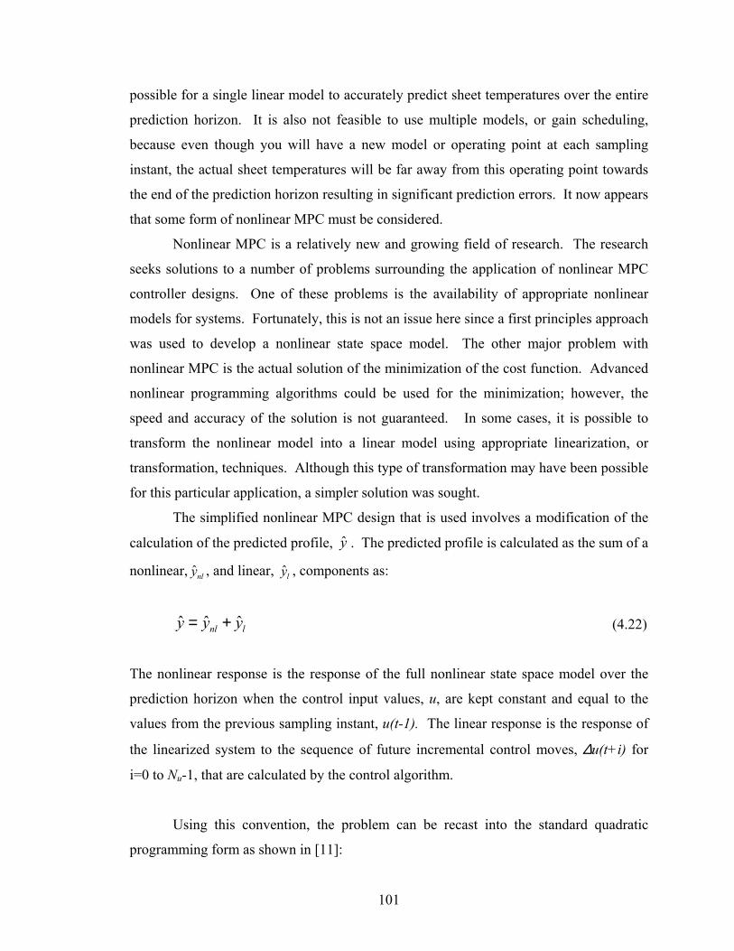
101
possible for a single linear model to accurately predict sheet temperatures over the entire
prediction horizon. It is also not feasible to use multiple models, or gain scheduling,
because even though you will have a new model or operating point at each sampling
instant, the actual sheet temperatures will be far away from this operating point towards
the end of the prediction horizon resulting in significant prediction errors. It now appears
that some form of nonlinear MPC must be considered.
Nonlinear MPC is a relatively new and growing field of research. The research
seeks solutions to a number of problems surrounding the application of nonlinear MPC
controller designs. One of these problems is the availability of appropriate nonlinear
models for systems. Fortunately, this is not an issue here since a first principles approach
was used to develop a nonlinear state space model. The other major problem with
nonlinear MPC is the actual solution of the minimization of the cost function. Advanced
nonlinear programming algorithms could be used for the minimization; however, the
speed and accuracy of the solution is not guaranteed. In some cases, it is possible to
transform the nonlinear model into a linear model using appropriate linearization, or
transformation, techniques. Although this type of transformation may have been possible
for this particular application, a simpler solution was sought.
The simplified nonlinear MPC design that is used involves a modification of the
calculation of the predicted profile, y . The predicted profile is calculated as the sum of a
nonlinear, ˆnly , and linear, ˆly , components as:
ˆ ˆ ˆnl ly y y= + (4.22)
The nonlinear response is the response of the full nonlinear state space model over the
prediction horizon when the control input values, u, are kept constant and equal to the
values from the previous sampling instant, u(t-1). The linear response is the response of
the linearized system to the sequence of future incremental control moves, ∆u(t+i) for
i=0 to Nu-1, that are calculated by the control algorithm.
Using this convention, the problem can be recast into the standard quadratic
programming form as shown in [11]:
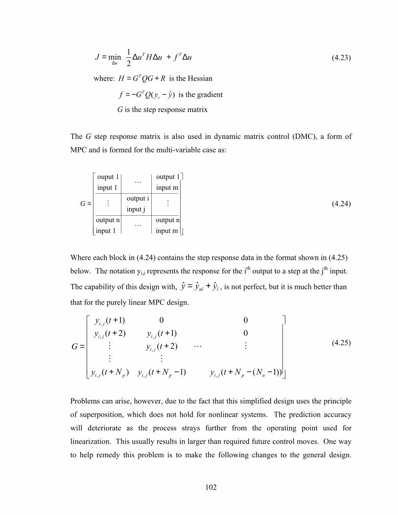
102
1min 2
T T
uJ u H u f u
∆= ∆ ∆ + ∆ (4.23)
where: TH G QG R= + is the Hessian
ˆ( )Trf G Q y y= − − is the gradient
G is the step response matrix
The G step response matrix is also used in dynamic matrix control (DMC), a form of
MPC and is formed for the multi-variable case as:
(4.24)
Where each block in (4.24) contains the step response data in the format shown in (4.25)
below. The notation yi,j represents the response for the ith output to a step at the jth input.
The capability of this design with, ˆ ˆ ˆnl ly y y= + , is not perfect, but it is much better than
that for the purely linear MPC design.
(4.25)
Problems can arise, however, due to the fact that this simplified design uses the principle
of superposition, which does not hold for nonlinear systems. The prediction accuracy
will deteriorate as the process strays further from the operating point used for
linearization. This usually results in larger than required future control moves. One way
to help remedy this problem is to make the following changes to the general design.
ouput 1 output 1input 1 input m
output iinput j
output n output ninput 1 input m
G
=
,
, ,
,
, , ,
( 1) 0 0( 2) ( 1) 0
( 2)
( ) ( 1) ( ( 1))
i j
i j i j
i j
i j p i j p i j p u
y ty t y t
y tG
y t N y t N y t N N
+ + + += + + − + − −
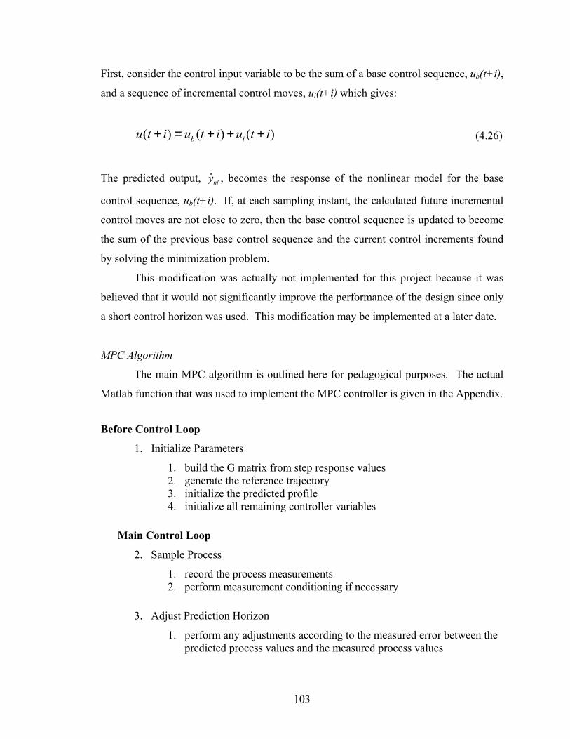
103
First, consider the control input variable to be the sum of a base control sequence, ub(t+i),
and a sequence of incremental control moves, ui(t+i) which gives:
( ) ( ) ( )b iu t i u t i u t i+ = + + + (4.26)
The predicted output, ˆnly , becomes the response of the nonlinear model for the base
control sequence, ub(t+i). If, at each sampling instant, the calculated future incremental
control moves are not close to zero, then the base control sequence is updated to become
the sum of the previous base control sequence and the current control increments found
by solving the minimization problem.
This modification was actually not implemented for this project because it was
believed that it would not significantly improve the performance of the design since only
a short control horizon was used. This modification may be implemented at a later date.
MPC Algorithm
The main MPC algorithm is outlined here for pedagogical purposes. The actual
Matlab function that was used to implement the MPC controller is given in the Appendix.
Before Control Loop
1. Initialize Parameters
1. build the G matrix from step response values 2. generate the reference trajectory 3. initialize the predicted profile 4. initialize all remaining controller variables
Main Control Loop
2. Sample Process
1. record the process measurements 2. perform measurement conditioning if necessary
3. Adjust Prediction Horizon
1. perform any adjustments according to the measured error between the predicted process values and the measured process values
104
4. Calculate Optimal Control Moves
1. first calculate the predicted error 2. solve the minimization problem to find the control moves
5. Send Control Moves
1. constrain control moves if necessary 2. send control moves to the process
6. Generate Predicted Profile
1. calculate the new predicted profile as a result of the new control moves
7. Update Variables
1. advance the predicted horizon by one sampling time increment 2. update the control move variables
8. Delay For One Sampling Instant
End of Control Loop
MPC Robustness
One of the problems with MPC is that it is generally not very robust.
Performance will deteriorate in the presence of modeling errors and external disturbances
acting on the system. Two modifications were made in order to improve the robustness
of the nonlinear MPC design. Both of these modifications occur within step 3 in the
MPC algorithm presented above.
The first modification is a polynomial filtering approach and involves the
following basic steps as suggested in [11]:
1. The error between the measured output, ym(t), and the predicted output, ˆ( )y t , is
structured as a polynomial of the form: 2
0 1 2( ) ... MMerror t e e t e t e t= + + + + (4.27)
where M is the order of the polynomial and a controller design parameter.
105
2. The coefficients of the polynomial in (4.27) are found using a least squares approach
with measured error data over a past finite horizon. The length of this horizon is another
tuning parameter.
3. The future predicted errors over the prediction horizon are found using the estimated
coefficients.
4. The predicted profile is then adjusted by adding the predicted errors from step 3 as a
correction term.
The authors in [11] state that this approach has been successfully applied in industrial
applications to remove the steady state offset resulting from model mismatch. I had great
difficulties, however, tuning the parameters of the polynomial filter. The order of the
polynomial was eventually chosen to be zero. In effect, the entire prediction profile is
shifted either up or down depending on past error values. The length of the time horizon
over which past error data was collected was chosen to be equal to the prediction horizon.
The second modification for robustness improvement was the addition of an
integration term in the algorithm. The integration term was not added to the error
signal, ˆry y− . It was instead added to another error signal, the difference between the
value of the desired setpoint, yr, and the measured process output, ym. This error is
integrated over time and added to a fictitious reference trajectory that is used for
calculating the predicted error profile. In effect, the fictitious reference trajectory is
continuously shifted until the actual measured output matches the true reference
trajectory. The integration is implemented in the discrete time MPC controller by adding
the following lines of code:
_ _ [ ( 0) ]
( ) ( ) _ for = 0 to r m
r r p
error sum error sum y t y kiy t i y t i error sum i N
= + + − ×+ = + + (4.28)
where ki is the integration constant and a tuning parameter. This technique works quite
well for “step-like” reference trajectories and even ramp reference signals even though
106
linear systems theory states that a system type of 2 (i.e. double integration) is required for
zero steady state error to ramp signals. An attempt was made to use double integration in
the design, but the tuning of the two integration constants proved to be very difficult.
MPC Tuning
It is worthwhile to discuss how some of the tuning parameters affect the
performance of the MPC controller. Aside from the tuning difficulties mentioned for the
polynomial error fitting and integration, the MPC tuning process is generally quite
intuitive and not all that difficult. The most important tuning parameters are the lengths
of the prediction and control horizons (Np and Nu respectively) and the weights on the
individual predicted errors and control moves terms in the cost function (Qi’s and Ri’s
respectively). As a general rule, the length of the prediction horizon should be long
enough such that the step response of the system reaches 99 percent of its steady state
value. Shorter prediction horizons can also be used if desired, but one must remember
that this will diminish the predictive capabilities of the controller. The length of the
control horizon can be set as desired. A longer control horizon results in more aggressive
control action as well as a more computationally demanding design. The Simplified
MPC (SMPC) controller (i.e. Nu = 1) is quite often an effective controller design.
The choice of the weights used in the cost functions are much more arbitrary. The
MPC design developed in this project used constant R values to place an equal weight on
all actuators. The values for the Q terms were generally constant although, at times,
heavier weights were used for earlier or later portions of the predicted error profile.
4.3.3 Simulation Results
The MPC controller design was evaluated by considering the same simulation
conditions and performance criteria that were used with the H∞ design. Figure 4.16
shows the results of the long-cycle simulation. It is clear from the results that the MPC
design fairs much better than the H∞ design when applied to the long-cycle setpoint. The
initial dynamic tracking behavior during the rising portion of the setpoint is quite good.
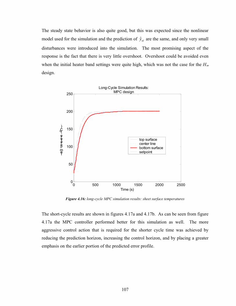
107
The steady state behavior is also quite good, but this was expected since the nonlinear
model used for the simulation and the prediction of ˆnly are the same, and only very small
disturbances were introduced into the simulation. The most promising aspect of the
response is the fact that there is very little overshoot. Overshoot could be avoided even
when the initial heater band settings were quite high, which was not the case for the H∞
design.
0 500 1000 1500 2000 25000
50
100
150
200
250Long-Cycle Simulation Results:
MPC design
Time (s)
Temperature (
oC)
top surface center line bottom surfacesetpoint
Figure 4.16: long-cycle MPC simulation results: sheet surface temperatures
The short-cycle results are shown in figures 4.17a and 4.17b. As can be seen from figure
4.17a the MPC controller performed better for this simulation as well. The more
aggressive control action that is required for the shorter cycle time was achieved by
reducing the prediction horizon, increasing the control horizon, and by placing a greater
emphasis on the earlier portion of the predicted error profile.
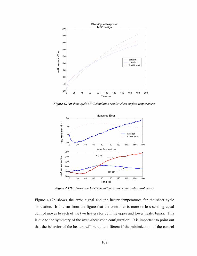
108
0 20 40 60 80 100 120 140 160 180 20020
40
60
80
100
120
140
160
180
200
Time (s)
Temperature (
oC)
Short-Cycle Response:MPC design
setpoint open loop closed loop
Figure 4.17a: short-cycle MPC simulation results: sheet surface temperatures
0 20 40 60 80 100 120 140 160 180-10
0
10
20Measured Error
Temperature (
oC)
top error bottom error
0 20 40 60 80 100 120 140 160 180660
680
700
720
740
760Heater Temperatures
Time (s)
Temperature (K) T2, T5
B2, B5
Figure 4.17b: short-cycle MPC simulation results: error and control moves
Figure 4.17b shows the error signal and the heater temperatures for the short cycle
simulation. It is clear from the figure that the controller is more or less sending equal
control moves to each of the two heaters for both the upper and lower heater banks. This
is due to the symmetry of the oven-sheet zone configuration. It is important to point out
that the behavior of the heaters will be quite different if the minimization of the control
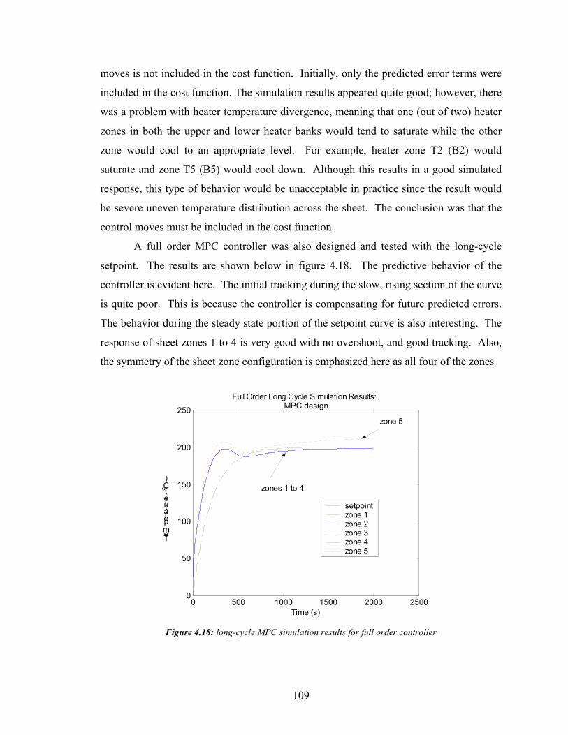
109
moves is not included in the cost function. Initially, only the predicted error terms were
included in the cost function. The simulation results appeared quite good; however, there
was a problem with heater temperature divergence, meaning that one (out of two) heater
zones in both the upper and lower heater banks would tend to saturate while the other
zone would cool to an appropriate level. For example, heater zone T2 (B2) would
saturate and zone T5 (B5) would cool down. Although this results in a good simulated
response, this type of behavior would be unacceptable in practice since the result would
be severe uneven temperature distribution across the sheet. The conclusion was that the
control moves must be included in the cost function.
A full order MPC controller was also designed and tested with the long-cycle
setpoint. The results are shown below in figure 4.18. The predictive behavior of the
controller is evident here. The initial tracking during the slow, rising section of the curve
is quite poor. This is because the controller is compensating for future predicted errors.
The behavior during the steady state portion of the setpoint curve is also interesting. The
response of sheet zones 1 to 4 is very good with no overshoot, and good tracking. Also,
the symmetry of the sheet zone configuration is emphasized here as all four of the zones
0 500 1000 1500 2000 25000
50
100
150
200
250Full Order Long Cycle Simulation Results:
MPC design
Time (s)
Temperature (
oC)
setpointzone 1 zone 2 zone 3 zone 4 zone 5
zones 1 to 4
zone 5
Figure 4.18: long-cycle MPC simulation results for full order controller
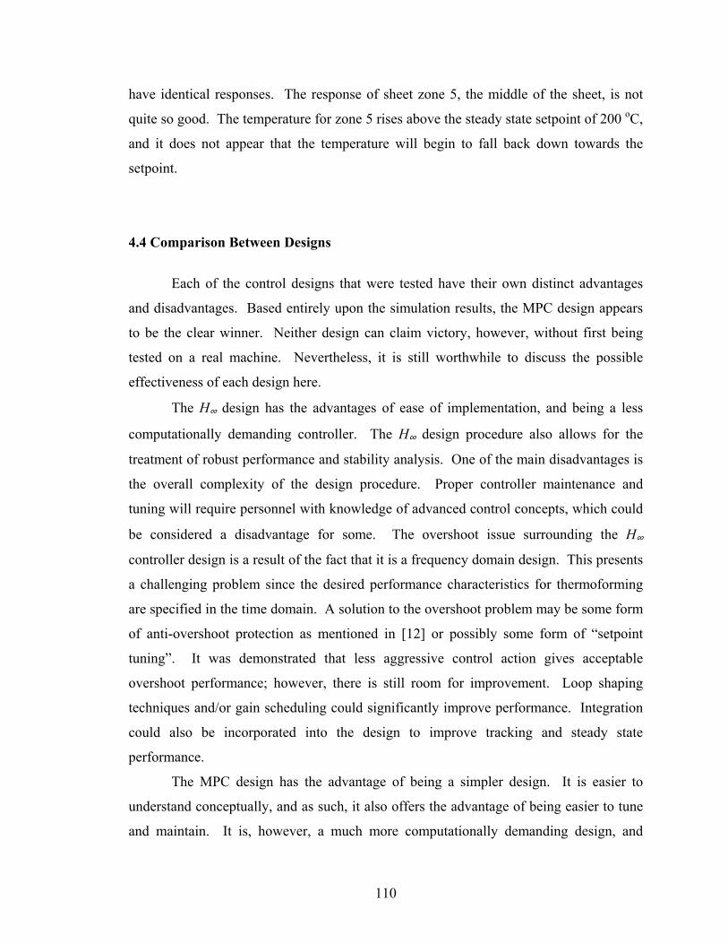
110
have identical responses. The response of sheet zone 5, the middle of the sheet, is not
quite so good. The temperature for zone 5 rises above the steady state setpoint of 200 oC,
and it does not appear that the temperature will begin to fall back down towards the
setpoint.
4.4 Comparison Between Designs
Each of the control designs that were tested have their own distinct advantages
and disadvantages. Based entirely upon the simulation results, the MPC design appears
to be the clear winner. Neither design can claim victory, however, without first being
tested on a real machine. Nevertheless, it is still worthwhile to discuss the possible
effectiveness of each design here.
The H∞ design has the advantages of ease of implementation, and being a less
computationally demanding controller. The H∞ design procedure also allows for the
treatment of robust performance and stability analysis. One of the main disadvantages is
the overall complexity of the design procedure. Proper controller maintenance and
tuning will require personnel with knowledge of advanced control concepts, which could
be considered a disadvantage for some. The overshoot issue surrounding the H∞
controller design is a result of the fact that it is a frequency domain design. This presents
a challenging problem since the desired performance characteristics for thermoforming
are specified in the time domain. A solution to the overshoot problem may be some form
of anti-overshoot protection as mentioned in [12] or possibly some form of “setpoint
tuning”. It was demonstrated that less aggressive control action gives acceptable
overshoot performance; however, there is still room for improvement. Loop shaping
techniques and/or gain scheduling could significantly improve performance. Integration
could also be incorporated into the design to improve tracking and steady state
performance.
The MPC design has the advantage of being a simpler design. It is easier to
understand conceptually, and as such, it also offers the advantage of being easier to tune
and maintain. It is, however, a much more computationally demanding design, and
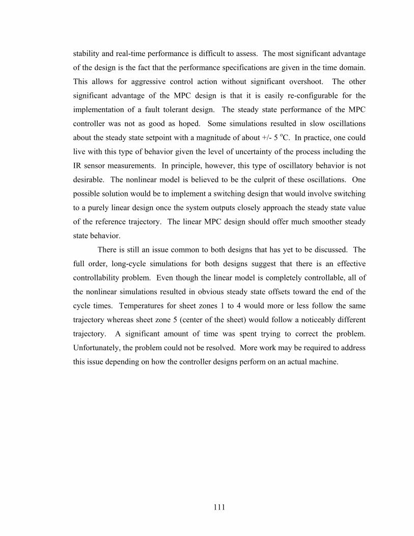
111
stability and real-time performance is difficult to assess. The most significant advantage
of the design is the fact that the performance specifications are given in the time domain.
This allows for aggressive control action without significant overshoot. The other
significant advantage of the MPC design is that it is easily re-configurable for the
implementation of a fault tolerant design. The steady state performance of the MPC
controller was not as good as hoped. Some simulations resulted in slow oscillations
about the steady state setpoint with a magnitude of about +/- 5 oC. In practice, one could
live with this type of behavior given the level of uncertainty of the process including the
IR sensor measurements. In principle, however, this type of oscillatory behavior is not
desirable. The nonlinear model is believed to be the culprit of these oscillations. One
possible solution would be to implement a switching design that would involve switching
to a purely linear design once the system outputs closely approach the steady state value
of the reference trajectory. The linear MPC design should offer much smoother steady
state behavior.
There is still an issue common to both designs that has yet to be discussed. The
full order, long-cycle simulations for both designs suggest that there is an effective
controllability problem. Even though the linear model is completely controllable, all of
the nonlinear simulations resulted in obvious steady state offsets toward the end of the
cycle times. Temperatures for sheet zones 1 to 4 would more or less follow the same
trajectory whereas sheet zone 5 (center of the sheet) would follow a noticeably different
trajectory. A significant amount of time was spent trying to correct the problem.
Unfortunately, the problem could not be resolved. More work may be required to address
this issue depending on how the controller designs perform on an actual machine.
112
5. Summary and Conclusions
This thesis documents the early development of a control strategy for the
thermoforming reheat process. The application of in-cycle control to sheet reheat was
considered in detail. The work was carried out with the primary objective of improved
material distribution via better pre-forming sheet temperature control in mind. In Section
1 the problem was defined and the possible benefits of closed loop control were
identified. A number of works that are relevant to the sheet reheat problem were cited.
Section 2 included a detailed description of the overall thermoforming process with
specific attention being given to the processing parameters that directly affect the sheet
reheat stage.
The process model that was used for in-cycle controller design was developed in
Section 3. It was found that a purely black box modeling approach was not appropriate
due to the difficulties in applying standard system identification techniques as well as the
large number of required system identification experiments. A first principles sheet
modeling approach along with a black box heater modeling approach proved to be more
practical. The nonlinear state space equations were presented as well as a number of
recommendations for model improvements, of which the most significant was better
representation of dynamic material properties.
Section 4 presented the details of H∞ and MPC in-cycle controller designs.
Simulation results indicate that the slow cooling dynamics of the ceramic heating
elements pose a major problem for the H∞ design. Without any time domain predictive
abilities, the H∞ controller is susceptible to significant overshoot as a result of the
nonlinear heater dynamics. The MPC simulation results are somewhat more promising in
that the overshoot problem is not a factor in the MPC design; however, further study into
real-time and stability issues is required. In conclusion, the performance of any in-cycle
control design will be dependant upon the reheat cycle time. Shorter cycle time
applications will have to rely more on adaptive cycle-to-cycle control and soft sensor
prediction since in-cycle control performance will be limited. That being said, it is
believed that in-cycle control has great potential for medium to long cycle thermoforming
113
applications. Hopefully, closed loop reheat control will eventually become mainstream
within the thermoforming industry.
Unfortunately, due to length restrictions, not all discussions could be included in
this thesis. Full detailed discussions of this work will be available in a future CIM report,
[26]. The CIM report will document the results of experimental testing of the controller
designs. It will also contain discussions on future recommendations and the integration
of this work with other thermoforming research work currently underway at McGill and
IMI.
114
Acknowledgements
I would like to express my sincere appreciation for all of those who helped me
complete my thesis research work. I would first like to acknowledge the cooperation
offered by IMI. My thesis work would not have been possible without the use of the
thermoforming equipment at IMI. I would like to recognize the financial support offered
by IMI, which allowed me to obtain all supplementary equipment and supplies required
for my experiments.
The people that I worked with in the Intelligent Forming Technologies Group at
IMI were very helpful. The support offered by Robert DiRaddo and Patrick Girard has
been greatly appreciated. I would also like to recognize the many technical discussions
with Nabil Aouf. Nabil was particularly helpful with the many different H∞ controller
designs that were considered. I would also like to acknowledge the support of Mitra
Yousefi, Denis Laroche, and Benoit Lanctot. I would not have been able to use the IMI
thermoforming simulation software without their gracious help. Finally, I would like to
thank Christian deGrandpre ; for his tireless efforts while helping me with all of the
experimental equipment setups. He never failed to answer my requests.
Last but not least I would like to thank my thesis supervisor, Benoit Boulet, for
his continuous guidance. I have greatly appreciated his technical and financial support.
His mentorship has made my stay at McGill an enjoyable and memorable experience.
115
Bibliography
[1] James L. Throne. “Technology of Thermoforming”, Hanser Publishers, 1996
[2] Adolf Illig. “Thermoforming: A Practical Guide”, Hanser Publishers, 2001
[3] John Florian. “Practical Thermoforming, Principles and Applications, Second Edition”, Marcel Dekker Inc., 1996
[4] J.P. Holman. “Heat Transfer, 8th Edition”, McGraw-Hill, 1997
[5] Robert Siegel, John R. Howell. “Thermal Radiation Heat Transfer, 3rd Edition”, Hemisphere Publishing, 1992
[6] D.G. Baird, D.I. Collais. “Polymer Processing Principles and Design”, Butterworth-Heinemann, 1995
[7] K. Zhou, J.C. Doyle. “Essentials of Robust Control”, Prentice Hall, 1998
[8] Benoit Boulet. “Robust Industrial Control, Course Notes Part 1: Model Predictive Control”, Coronado Systems, 2000
[9] Benoit Boulet. “Robust Industrial Control, Course Notes Part 2: Robust and Optimal Control”, Coronado Systems, 2000
[10] Gary J. Balas, John C. Doyle, Keith Glover, Andy Packard, Roy Smith. “Matlab User’s Guide: µ-Analysis and Synthesis Toolbox, Version 3”, The Math Works, 1998
[11] Murali Gopinathan, Raman K. Mehra, Joseph C. Runkle. “Hot Isostatic Pressing Furnaces, Their Modeling and Predictive Fault-Tolerant Control”, in IEEE Control Systems Magazine, pp. 67-82, December 2000
[12] Charles Schaper, Mehrdad Moslehi, Krishna Saraswat, Thomas Kailath. “Control of MMST RTP: Repeatability, Uniformity, and Integration for Flexible Manufacturing”, in IEEE Transactions on Semiconductor Manufacturing, Vol 7, No. 2, May 1994
[13] Poogyeon Park, Charles Schaper, Thomas Kailath. “Control Strategy for Temperature Tracking in Rapid Thermal Processing of Semiconductor Wafers”, in Proceedings of the 31st Conference on Decision and Control, pp. 2568-2572, December 1992
[14] Young Man Cho, Thomas Kailath. “Model Identification in Rapid Thermal Processing Systems”, in IEEE Transactions on Semiconductor Manufacturing, Vol 6, No. 3, August 1993
[15] A. Yousefi, A. Bendada, R. DiRaddo. “Improved Modeling for the Reheat Phase in Thermoforming Through an Uncertainty Treatment of the Key Parameters”, in SPE ANTEC, May 2001
[16] W. Michaeli, J. van Marwick. “Automation of the Thermoforming Process by a Wall Thickness Closed-Loop Control”, in SPE ANTEC, 1996
[17] Rickey Dubay, Yash P. Gupta, Adam C. Bell. “Predictive Control of Plastic Melt in Heated Zones With Insulation”, in Journal of Injection Molding Technology, Vol. 2, No. 1, pp. 37-45, March 1998
116
[18] Suman Banerjee, J. Vernon Cole, Klavs F. Jensen. “ Nonlinear Model Reduction Strategies for Rapid Thermal Processing Systems”, in IEEE Transactions on Semiconductor Manufacturing, Vol. 11, No. 2, May 1998
[19] Jalil Kamali, Robert L. Kosut. “Time-Varying Optimal Controller for Rapid Thermal Processing (RTP) Reactors”, in Proceedings of the 36th Conference on Decision and Control, pp. 2541-2542, December 1997
[20] Robin DeKeyser, James Donald III. “Model Based Predictive Control n RTP Semiconductor Manufacturing”, in Proceedings of the 1999 IEEE International Conference on Control Applications, pp. 1636-1641, August 1999
[21] Arvind Srinivasan, Celal Batur, Robert Veillette, Bruce N. Rosenthal, Walter M.B. Duval. “Projective Control Design for Muli-Zone Crystal Growth Furnace”, in IEEE Transactions on Control Systems Technology, Vol. 2, No. 2, June 1994
[22] Mukul Agarwal. “ A Systematic Classification of Neural-Network-Based Control”, in The 3rd IEEE Conference on Control Applications, August 1994
[23] Sang Kyung Lee, Jong Hae Kim, Oh Do Chang, Hong Bae Park. “Robust Controller Design for RTP using Structured Uncertainty Approach”, in SICE, July 1999
[24] Tarek Alaeddine, Haris Doumanidis. “ Distributed Parameter Thermal Controllability – the Inverse Heat Conduction Problem in Materials Processing, in ACC, 2002
[25] R. W. DiRaddo, A. Garcia-Rejon. "In-cycle Deterministic and Stochastic Dynamics of Extrusion Blow Molding", in Intern. Polymer Processing VII, pp. 257-266, 1992
[26] CIM report No. CIM-TR02-01
117
Appendix
Matlab code for H∞ controller design: h_inf_build_model_unstruc.m 118
Matlab code for MPC controller design: mpc_controller_nl.m 121
Simulink model diagrams 127
Linearized state space modeling equations 133
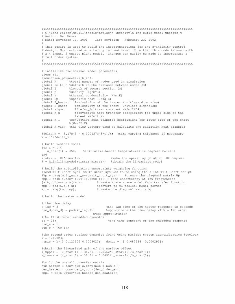
118
%%%%%%%%%%%%%%%%%%%%%%%%%%%%%%%%%%%%%%%%%%%%%%%%%%%%%%%%%%%%%%%%%%%%%%%%%%%%%%%%%%% C:\Bens Folder\McGill\thesis\matlab\h infinity\h_inf_build_model_unstruc.m% Author: Ben Moore% Date: November 13, 2001 last revision: February 23, 2002%% This script is used to build the interconnections for the H-infinity control% design. Unstructured uncertainty is used here. Note that this code is used with% a 4 input, 2 output plant model. Changes can easily be made to incorporate a% full order system.%%%%%%%%%%%%%%%%%%%%%%%%%%%%%%%%%%%%%%%%%%%%%%%%%%%%%%%%%%%%%%%%%%%%%%%%%%%%%%%%%%%
% initialize the nominal model parametersclear all;simulation_parameters_h_inf;global N %total number of nodes used in simulationglobal delta_h %delta_h is the distance between nodes (m)global l %length of square section (m)global p %density (kg/m^3)global k %thermal conductivity (W/m.K)global Cp %specific heat (J/kg.K)global E_heater %emissivity of the heater (unitless dimension)global E_sheet %emissivity of the sheet (unitless dimension)global sigma %Stefan_Boltzman constant (W/m^2K^4)global h_u %convective heat transfer coefficient for upper side of the
%sheet (W/m^2.K)global h_l %convective heat transfer coefficient for lower side of the sheet
%(W/m^2.K)global F_view %the view vactors used to calculate the radiation heat transfer
%delta_h = (3.17e-3 - 0.000457e-3*t)/N; %time varying thickness if necessaryV = l^2*delta_h;
% build nominal modelfor i = 1:4
u_star(i) = 350; %initialize heater temperatures in degrees Celciusendx_star = 100*ones(1,N); %make the operating point at 100 degreesP = h_inf_lin_model(u_star,x_star); %obtain the linearized model
% build the multiplicative uncertainty weighting function%load mult_uncrt_sys; %mult_uncrt_sys was found using the h_inf_mult_uncrt script%Wp = daug(mult_uncrt_sys,mult_uncrt_sys); %create the diagonal matrix Wptmp = tf(0.5,conv([200 1],[200 1])); %the uncertainty at low frequencies[a,b,c,d]=ssdata(tmp); %create state space model from transfer functiontmp = pck(a,b,c,d); %convert to mu toolbox model formatWp = daug(tmp,tmp); %create the diagonal matrix Wp
% build the heater model
% the time delayt_lag = 5; %the lag time of the heater response in secondsnum_d,den_d] = pade(t_lag,1); %approximate the time delay with a 1st order
%Pade approximation%the first order embedded dynamicstc = 25; %the time constant of the embedded responsenum_e = 1;den_e = [tc 1];
%the second order surface dynamics found using matlabs system identification %toolboxk = 1/1.023;num_s = k*[0 0.123355 0.000302]; den_s = [1 0.085266 0.000295];
%obtain the linearized gain of the surface offsetk_upper = (u_star(1) + 31.51 + 0.0662*u_star(1))/u_star(1);k_lower = (u_star(3) + 35.51 + 0.0452*u_star(3))/u_star(3);
%build the overall transfer matrixnum_heater = conv(num_s,conv(num_d,num_e));den_heater = conv(den_s,conv(den_d,den_e));tmp1 = tf(k_upper*num_heater,den_heater);
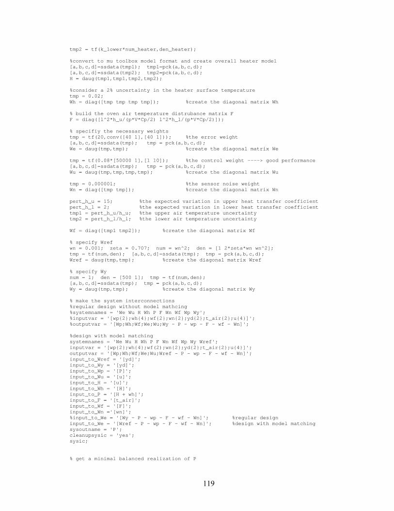
119
tmp2 = tf(k_lower*num_heater,den_heater);
%convert to mu toolbox model format and create overall heater model[a,b,c,d]=ssdata(tmp1); tmp1=pck(a,b,c,d);[a,b,c,d]=ssdata(tmp2); tmp2=pck(a,b,c,d);H = daug(tmp1,tmp1,tmp2,tmp2);
%consider a 2% uncertainty in the heater surface temperaturetmp = 0.02;Wh = diag([tmp tmp tmp tmp]); %create the diagonal matrix Wh
% build the oven air temperature distrubance matrix FF = diag([l^2*h_u/(p*V*Cp/2) l^2*h_l/(p*V*Cp/2)]);
% specifiy the necessary weightstmp = tf(20,conv([40 1],[40 1])); %the error weight[a,b,c,d]=ssdata(tmp); tmp = pck(a,b,c,d);We = daug(tmp,tmp); %create the diagonal matrix We
tmp = tf(0.08*[50000 1],[1 10]); %the control weight ----> good performance[a,b,c,d]=ssdata(tmp); tmp = pck(a,b,c,d);Wu = daug(tmp,tmp,tmp,tmp); %create the diagonal matrix Wu
tmp = 0.000001; %the sensor noise weightWn = diag([tmp tmp]); %create the diagonal matrix Wn
pert_h_u = 15; %the expected variation in upper heat transfer coefficientpert_h_l = 2; %the expected variation in lower heat transfer coefficienttmp1 = pert_h_u/h_u; %the upper air temperature uncertaintytmp2 = pert_h_l/h_l; %the lower air temperature uncertainty
Wf = diag([tmp1 tmp2]); %create the diagonal matrix Wf
% specify Wrefwn = 0.001; zeta = 0.707; num = wn^2; den = [1 2*zeta*wn wn^2];tmp = tf(num,den); [a,b,c,d]=ssdata(tmp); tmp = pck(a,b,c,d);Wref = daug(tmp,tmp); %create the diagonal matrix Wref
% specify Wynum = 1; den = [500 1]; tmp = tf(num,den);[a,b,c,d]=ssdata(tmp); tmp = pck(a,b,c,d);Wy = daug(tmp,tmp); %create the diagonal matrix Wy
% make the system interconnections%regular design without model mathcing%systemnames = 'We Wu H Wh P F Wn Wf Wp Wy';%inputvar = '[wp{2};wh{4};wf{2};wn{2};yd{2};t_air{2};u{4}]';%outputvar = '[Wp;Wh;Wf;We;Wu;Wy - P - wp - F - wf - Wn]';
%design with model matchingsystemnames = 'We Wu H Wh P F Wn Wf Wp Wy Wref';inputvar = '[wp{2};wh{4};wf(2);wn{2};yd{2};t_air{2};u{4}]';outputvar = '[Wp;Wh;Wf;We;Wu;Wref - P - wp - F - wf - Wn]';input_to_Wref = '[yd]';input_to_Wy = '[yd]';input_to_Wp = '[P]';input_to_Wu = '[u]';input_to_H = '[u]';input_to_Wh = '[H]';input_to_P = '[H + wh]';input_to_F = '[t_air]';input_to_Wf = '[F]';input_to_Wn ='[wn]';%input_to_We = '[Wy - P - wp - F - wf - Wn]'; %regular designinput_to_We = '[Wref - P - wp - F - wf - Wn]'; %design with model matchingsysoutname = 'P';cleanupsysic = 'yes';sysic;
% get a minimal balanced realization of P
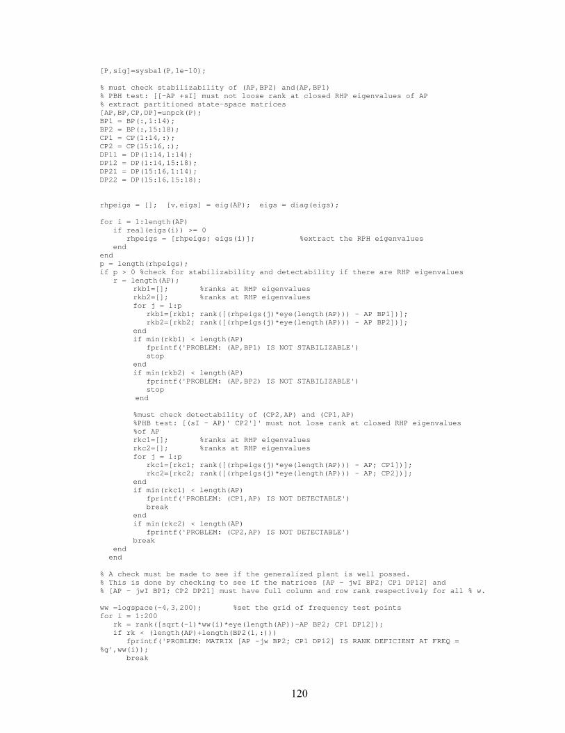
120
[P,sig]=sysbal(P,1e-10);
% must check stabilizability of (AP,BP2) and(AP,BP1)% PBH test: [[-AP +sI] must not loose rank at closed RHP eigenvalues of AP% extract partitioned state-space matrices[AP,BP,CP,DP]=unpck(P);BP1 = BP(:,1:14);BP2 = BP(:,15:18);CP1 = CP(1:14,:);CP2 = CP(15:16,:);DP11 = DP(1:14,1:14);DP12 = DP(1:14,15:18);DP21 = DP(15:16,1:14);DP22 = DP(15:16,15:18);
rhpeigs = []; [v,eigs] = eig(AP); eigs = diag(eigs);
for i = 1:length(AP)if real(eigs(i)) >= 0
rhpeigs = [rhpeigs; eigs(i)]; %extract the RPH eigenvaluesend
endp = length(rhpeigs);if p > 0 %check for stabilizability and detectability if there are RHP eigenvalues
r = length(AP);rkb1=[]; %ranks at RHP eigenvaluesrkb2=[]; %ranks at RHP eigenvaluesfor j = 1:p
rkb1=[rkb1; rank([(rhpeigs(j)*eye(length(AP))) - AP BP1])];rkb2=[rkb2; rank([(rhpeigs(j)*eye(length(AP))) - AP BP2])];
endif min(rkb1) < length(AP)
fprintf('PROBLEM: (AP,BP1) IS NOT STABILIZABLE')stop
endif min(rkb2) < length(AP)
fprintf('PROBLEM: (AP,BP2) IS NOT STABILIZABLE')stop
end
%must check detectability of (CP2,AP) and (CP1,AP)%PHB test: [(sI - AP)' CP2']' must not lose rank at closed RHP eigenvalues%of APrkc1=[]; %ranks at RHP eigenvaluesrkc2=[]; %ranks at RHP eigenvaluesfor j = 1:p
rkc1=[rkc1; rank([(rhpeigs(j)*eye(length(AP))) - AP; CP1])];rkc2=[rkc2; rank([(rhpeigs(j)*eye(length(AP))) - AP; CP2])];
endif min(rkc1) < length(AP)
fprintf('PROBLEM: (CP1,AP) IS NOT DETECTABLE')break
endif min(rkc2) < length(AP)
fprintf('PROBLEM: (CP2,AP) IS NOT DETECTABLE')break
endend
% A check must be made to see if the generalized plant is well possed.% This is done by checking to see if the matrices [AP - jwI BP2; CP1 DP12] and% [AP - jwI BP1; CP2 DP21] must have full column and row rank respectively for all % w.
ww =logspace(-4,3,200); %set the grid of frequency test pointsfor i = 1:200
rk = rank([sqrt(-1)*ww(i)*eye(length(AP))-AP BP2; CP1 DP12]);if rk < (length(AP)+length(BP2(1,:)))
fprintf('PROBLEM: MATRIX [AP -jw BP2; CP1 DP12] IS RANK DEFICIENT AT FREQ =%g',ww(i));
break
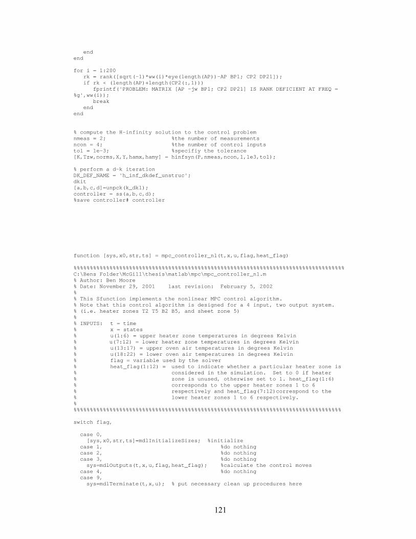
121
endend
for i = 1:200rk = rank([sqrt(-1)*ww(i)*eye(length(AP))-AP BP1; CP2 DP21]);if rk < (length(AP)+length(CP2(:,1)))
fprintf('PROBLEM: MATRIX [AP -jw BP1; CP2 DP21] IS RANK DEFICIENT AT FREQ =%g',ww(i));
breakend
end
% compute the H-infinity solution to the control problemnmeas = 2; %the number of measurementsncon = 4; %the number of control inputstol = 1e-3; %specifiy the tolerance[K,Tzw,norms,X,Y,hamx,hamy] = hinfsyn(P,nmeas,ncon,1,1e3,tol);
% perform a d-k iterationDK_DEF_NAME = 'h_inf_dkdef_unstruc';dkit[a,b,c,d]=unpck(k_dk1);controller = ss(a,b,c,d);%save controller# controller
function [sys,x0,str,ts] = mpc_controller_nl(t,x,u,flag,heat_flag)
%%%%%%%%%%%%%%%%%%%%%%%%%%%%%%%%%%%%%%%%%%%%%%%%%%%%%%%%%%%%%%%%%%%%%%%%%%%%%%%%%%%C:\Bens Folder\McGill\thesis\matlab\mpc\mpc_controller_nl.m% Author: Ben Moore% Date: November 29, 2001 last revision: February 5, 2002%% This Sfunction implements the nonlinear MPC control algorithm.% Note that this control algorithm is designed for a 4 input, two output system.% (i.e. heater zones T2 T5 B2 B5, and sheet zone 5)%% INPUTS: t = time% x = states% u(1:6) = upper heater zone temperatures in degrees Kelvin% u(7:12) = lower heater zone temperatures in degrees Kelvin% u(13:17) = upper oven air temperatures in degrees Kelvin% u(18:22) = lower oven air temperatures in degrees Kelvin% flag = variable used by the solver% heat_flag(1:12) = used to indicate whether a particular heater zone is% considered in the simulation. Set to 0 if heater% zone is unused, otherwise set to 1. heat_flag(1:6)% corresponds to the upper heater zones 1 to 6% respectively and heat_flag(7:12)correspond to the% lower heater zones 1 to 6 respectively.%%%%%%%%%%%%%%%%%%%%%%%%%%%%%%%%%%%%%%%%%%%%%%%%%%%%%%%%%%%%%%%%%%%%%%%%%%%%%%%%%%%
switch flag,
case 0,[sys,x0,str,ts]=mdlInitializeSizes; %initialize
case 1, %do nothingcase 2, %do nothingcase 3, %do nothing
sys=mdlOutputs(t,x,u,flag,heat_flag); %calculate the control movescase 4, %do nothingcase 9,
sys=mdlTerminate(t,x,u); % put necessary clean up procedures here
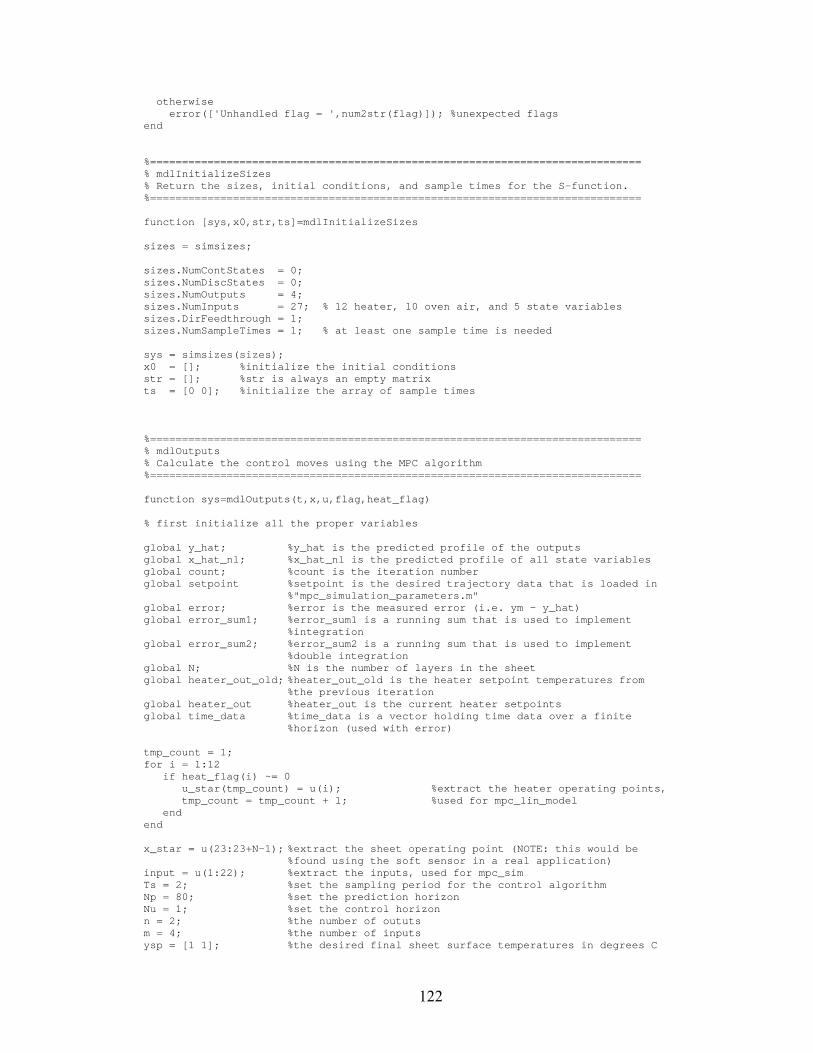
122
otherwiseerror(['Unhandled flag = ',num2str(flag)]); %unexpected flags
end
%=============================================================================% mdlInitializeSizes% Return the sizes, initial conditions, and sample times for the S-function.%=============================================================================
function [sys,x0,str,ts]=mdlInitializeSizes
sizes = simsizes;
sizes.NumContStates = 0;sizes.NumDiscStates = 0;sizes.NumOutputs = 4;sizes.NumInputs = 27; % 12 heater, 10 oven air, and 5 state variablessizes.DirFeedthrough = 1;sizes.NumSampleTimes = 1; % at least one sample time is needed
sys = simsizes(sizes);x0 = []; %initialize the initial conditionsstr = []; %str is always an empty matrixts = [0 0]; %initialize the array of sample times
%=============================================================================% mdlOutputs% Calculate the control moves using the MPC algorithm%=============================================================================
function sys=mdlOutputs(t,x,u,flag,heat_flag)
% first initialize all the proper variables
global y_hat; %y_hat is the predicted profile of the outputsglobal x_hat_nl; %x_hat_nl is the predicted profile of all state variablesglobal count; %count is the iteration numberglobal setpoint %setpoint is the desired trajectory data that is loaded in
%"mpc_simulation_parameters.m"global error; %error is the measured error (i.e. ym - y_hat)global error_sum1; %error_sum1 is a running sum that is used to implement
%integrationglobal error_sum2; %error_sum2 is a running sum that is used to implement
%double integrationglobal N; %N is the number of layers in the sheetglobal heater_out_old; %heater_out_old is the heater setpoint temperatures from
%the previous iterationglobal heater_out %heater_out is the current heater setpointsglobal time_data %time_data is a vector holding time data over a finite
%horizon (used with error)
tmp_count = 1;for i = 1:12
if heat_flag(i) ~= 0u_star(tmp_count) = u(i); %extract the heater operating points,tmp_count = tmp_count + 1; %used for mpc_lin_model
endend
x_star = u(23:23+N-1); %extract the sheet operating point (NOTE: this would be%found using the soft sensor in a real application)
input = u(1:22); %extract the inputs, used for mpc_simTs = 2; %set the sampling period for the control algorithmNp = 80; %set the prediction horizonNu = 1; %set the control horizonn = 2; %the number of oututsm = 4; %the number of inputsysp = [1 1]; %the desired final sheet surface temperatures in degrees C
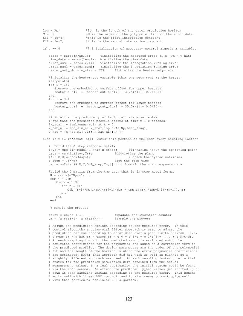
123
len = Np; %len is the length of the error prediction horizonM = 0; %M is the order of the polynomial fit for the error dataKi1 = 1e-4; %this is the first integration constantKi2 = 5e-2; %this is the second integration constant
if t == 0 %% initialization of necessary control algorithm variables
error = zeros(n*Np,1); %initialize the measured error (i.e. ym - y_hat)time_data = zeros(len,1); %initialize the time dataerror_sum1 = zeros(2,1); %initialize the integration running errorerror_sum2 = error_sum1; %initialize the integration running errorheater_out_old = u_star - 273; %intialize the heater setpoints
%initialize the heater_out variable (this one gets sent as the heater%setpoints)for i = 1:2
%remove the embedded to surface offset for upper heatersheater_out(i) = (heater_out_old(i) - 31.5)/(1 + 0.0662);
endfor i = 3:4
%remove the embedded to surface offset for lower heatersheater_out(i) = (heater_out_old(i) - 35.5)/(1 + 0.0425);
end
%initialize the predicted profile for all state variables%Note that the predicted profile starts at time t = 0 seconds.%x_star = Tamb*ones(N,1) at t = 0x_hat_nl = mpc_sim_nl(x_star,input,Ts,Np,heat_flag);y_hat = [x_hat_nl(:,1); x_hat_nl(:,N)];
else if t >= Ts*count %%%% enter this portion of the code every sampling instant
% build the G step response matrixlsys = mpc_lin_model(u_star,x_star); %linearize about the operating pointdsys = samhld(lsys,Ts); %discretize the plant[A,B,C,D]=unpck(dsys); %unpack the system matriciesT_step = Ts*Np; %set the step timetmp = ss2step(A,B,C,D,T_step,Ts,[],n); %obtain the step response data
%build the G matrix from the tmp data that is in step model formatG = zeros(n*Np,m*Nu);for j = 1:m
for k = 1:Nufor r = 1:n
G(k+(r-1)*Np:r*Np,k+(j-1)*Nu) = tmp(r:n:(n*(Np-k+1)-(n-r)),j);end
endend
% sample the process
count = count + 1; %upadate the iteration counterym = [x_star(1) x_star(N)]; %sample the process
% Adjust the prediction horizon according to the measured error. In this% control algorithm a polynomial filter approach is used to adjust the% prediction horizon according to error data over a past finite horizon. (i.e.% y_meas(t) - y_hat(t) = error(t) = e_0 + e_1*t + e_2*t^2 + .... + e_N*t^N).% At each sampling instant, the predicted error is evaluated using the% estimated coefficients for the polynomial and added as a correction term to% the predicted profile. The design parameters are the order of the polynomial% fit and the length of the horizon in which the error polynomial coefficients% are estimated. NOTE: This approach did not work as well as planned so a% slightly different approach was used. At each sampling instant the initial% states for the prediction simulation were obtained from the actual% measurement values. In a real application the initial states would be found% via the soft sensor. In effect the predicted y_hat values get shifted up or% down at each sampling instant according to the measured error. This scheme% works well with linear MPC control, and it also seems to work quite well% with this particular nonlinear MPC algorithm.
124
%update the error prediction vectorif count > len
for i = 1:len-1error(i) = error(i+1);
endfor i = len+1:n*len-1
error(i) = error(i+1);endfor i = 1:len-1
time_data(i) = time_data(i+1);enderror(len) = ym(1) - y_hat(1);error(2*len) = ym(2) - y_hat(Np+2);time_data(len) = Ts*count;
elseerror(count) = ym(1) - y_hat(1);error(count + len) = ym(2) - y_hat(Np+2);time_data(count) = Ts*count;
end
%now fit the error%obtain the coefficients for the upper sheet surfacecoef11 = polyfit(time_data,error(1:len),M);%obtain the coefficients for the lower sheet surfacecoef22 = polyfit(time_data,error(len+1:2*len),M);
%now generate the predicted error over the new prediction horizontime_data_fit = Ts*(count+1):Ts:Ts*(count+n*Np);error_fit1 = polyval(coef11,time_data_fit);error_fit2 = polyval(coef22,time_data_fit);
%Now add the predicted error to the predicted profile. As mentioned above this%approach did not work.for i = 2:Np+1
y_hat(i) = y_hat(i) + error_fit1(i-1);y_hat(i+Np+1) = y_hat(i+Np+1) + error_fit2(i-1);
end
% generate the setpoint trajectory
for i = 1:Np+1y(i) = ysp(1)*setpoint(Ts*(count+i-1),2);y(i+Np+1) = ysp(2)*setpoint(Ts*(count+i-1),2);
end
%Integration can be implemented by adjusting a virtual setpoint trajectory that%is used in the calculation of the optimal control moves. The idea is that an%integration term is added to this virtual setpoint trajectory until the process%tracks the actual setpoint trajectory.
error_sum1(1) = error_sum1(1) + ((ym(1) - 273) - y(1))*Ki1;error_sum1(2) = error_sum1(2) + ((ym(2) - 273) - y(Np+2))*Ki1;
%Note that double integration was finally not used since it was very difficult%to find the right combination of integration constants that gave a smooth%response. In theory double integration should be used to track ramp inputs.%Zero steady state error for ramp inputs requires a system type number of 2.%This is not easy to implement here though.
error_sum2(1) = error_sum2(1) + error_sum1(1)*Ki2;error_sum2(2) = error_sum2(2) + error_sum1(2)*Ki2;
for i = 1:Np+1y(i) = y(i) - error_sum1(1); %for double integration add error_sum2y(i+Np+1) = y(i) - error_sum1(2);
end
% calculate the optimal control moves
%generate the predicted errorpred_error = zeros(2*Np,1);
125
for i = 1:Nppred_error(i) = y(i+1) - (y_hat(i+1) - 273);
endfor i = Np+1:n*Np
pred_error(i) = y(i+2) - (y_hat(i+2) - 273);end
%Q is a diagonal matrix containing the weights on the individual error termsQ = 1e-4*eye(length(G(:,1)));for i = 1:Np
Q(i,i) = 1e-4*i^4; %put a heavier weight on the later time stepsQ(i + Np,i + Np) = Q(i,i);
end
R = 1e-4*eye(m*Nu); %also put a weight on each individual heater zone
H = G'*Q*G + R; %H is the hessianf = -G'*Q*pred_error; %f is the gradientA = [eye(m*Nu); -eye(m*Nu)];%A is used in the quadprog calldelta_u_max = 1*Ts*ones(m*Nu,1); %constrain the positive control movesdelta_u_min = 0.35*Ts*ones(m*Nu,1);%constrain the negative control movesb = [delta_u_max; delta_u_min]; %b is used in the quadprog calldelta_u = quadprog(H,f,A,b); %solve the quadratic programming problemy_lin = G*delta_u; %calculate the response of the linear plant
%update the heater outputs by adding the control movesdummy = delta_u(1:Nu:m*Nu);for i = 1:m
heater_out(i) = heater_out_old(i) + dummy(i);if heater_out(i) > 550
heater_out(i) = 550; %constrain the heater temperatures if necessaryend
endheater_out_old = heater_out; %update the heater_out_old variable
%the heater surface temperature offset must be removed firstfor i = 1:2
heater_out(i) = (heater_out_old(i) - 31.5)/(1 + 0.0662);endfor i = 3:4
heater_out(i) = (heater_out_old(i) - 35.5)/(1 + 0.0425);end
% generate the predicted profileXo = x_star; %the initial states for the current prediction are
%the states that are predicted by the soft sensorinput(2) = heater_out_old(1)+273; %Changed on Feb. 3 Before the
%heater_out_old variable was obtained from%measured heater temperatures. Without
input(5) = heater_out_old(2)+273; %change there was significant ocsil% about the setpoint at steady state.
input(2+6) = heater_out_old(3)+273; input(5+6) = heater_out_old(4)+273;
x_hat_nl = mpc_sim_nl(Xo,input,Ts,Np,heat_flag); %simulate non linear responsey_hat = [x_hat_nl(:,1); x_hat_nl(:,N)]; %extract surface temperatures
%add the linear responsefor i = 2:(Np+1)
y_hat(i) = y_hat(i) + y_lin(i-1);x_hat_nl(i,1) = y_hat(i);
endfor i = (Np+3):(n*Np+n)
y_hat(i) = y_hat(i) + y_lin(i-2);x_hat_nl(i,N) = y_hat(i);
end
% adjust the prediction horizon by one sampling instanty_hat(Np+1) = y_hat(Np);for i = 1:(Np)
y_hat(i) = y_hat(i+1);end
126
y_hat(n*Np+n) = y_hat(n*Np+n-1);for i = (Np+2):(n*Np+n-1)
y_hat(i) = y_hat(i+1);end
else
%%%%%%%%%%%%%%%%%% delay for one sampling period %%%%%%%%%%%%%%%%%
end
end
sys = heater_out; %send the control moves to the plant
%=============================================================================% mdlTerminate% Perform any end of simulation tasks.%=============================================================================%function sys=mdlTerminate(t,x,u)
global count; count = 0; %reset the count variablesys = [];
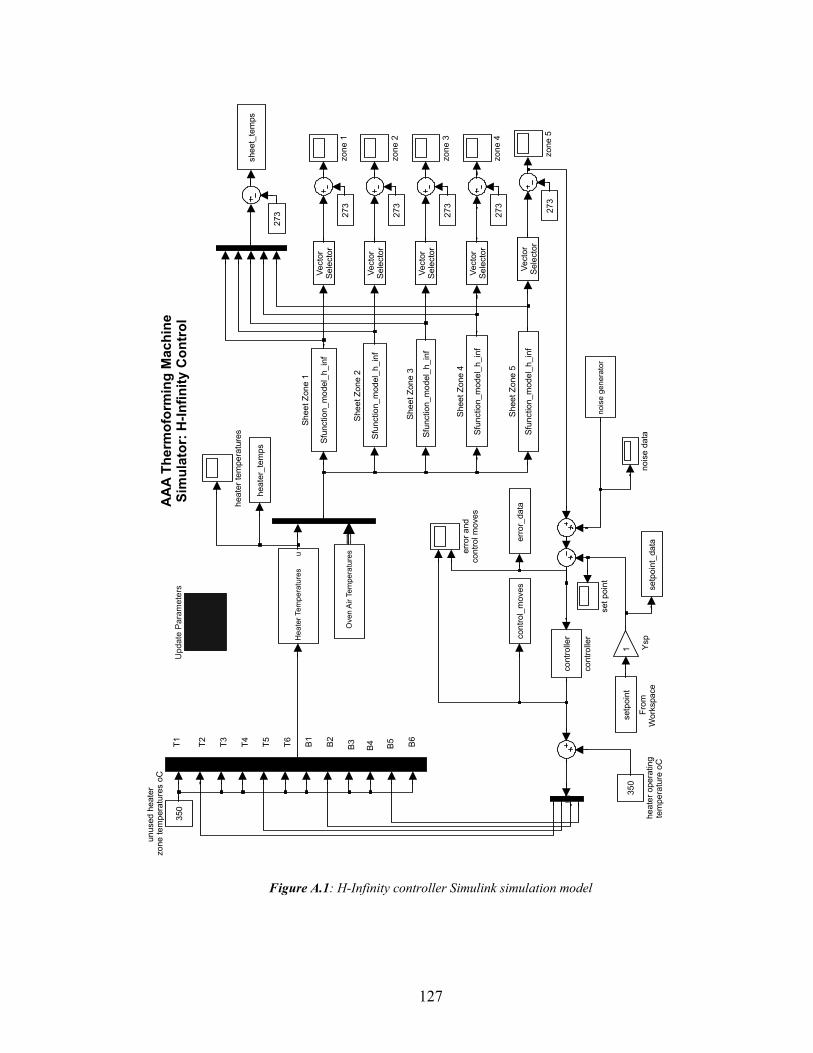
127
AA
A Th
erm
ofor
min
g M
achi
neSi
mul
ator
: H-In
finity
Con
trol
T1 T2 T3 T4 T5 T6 B1 B2 B3 B4 B5 B6
zone
5
zone
4
zone
3
zone
2
zone
1
350
unus
ed h
eate
r zo
ne te
mpe
ratu
res
oC
set p
oint
nois
e da
ta
heat
er te
mpe
ratu
res
350
heat
er o
pera
ting
tem
pera
ture
oC
erro
r and
cont
rol m
oves
cont
rolle
r
cont
rolle
r
1 Ysp
? ?
?
Upd
ate
Para
met
ers
cont
rol_
mov
eser
ror_
data
heat
er_t
emps
setp
oint
_dat
a
shee
t_te
mps
nois
e ge
nera
tor
Ove
n Ai
r Tem
pera
ture
s
Hea
ter T
empe
ratu
res
u
Sfun
ctio
n_m
odel
_h_i
nf
Shee
t Zon
e 5
Sfun
ctio
n_m
odel
_h_i
nf
Shee
t Zon
e 4
Sfun
ctio
n_m
odel
_h_i
nf
Shee
t Zon
e 3
Sfun
ctio
n_m
odel
_h_i
nf
Shee
t Zon
e 2
Sfun
ctio
n_m
odel
_h_i
nf
Shee
t Zon
e 1
Vect
orSe
lect
or
Vect
orSe
lect
or
Vect
orSe
lect
or
Vect
orSe
lect
or
Vect
orSe
lect
or
setp
oint
From
Wor
kspa
ce
273 27
3
273
273
273
273
Figure A.1: H-Infinity controller Simulink simulation model
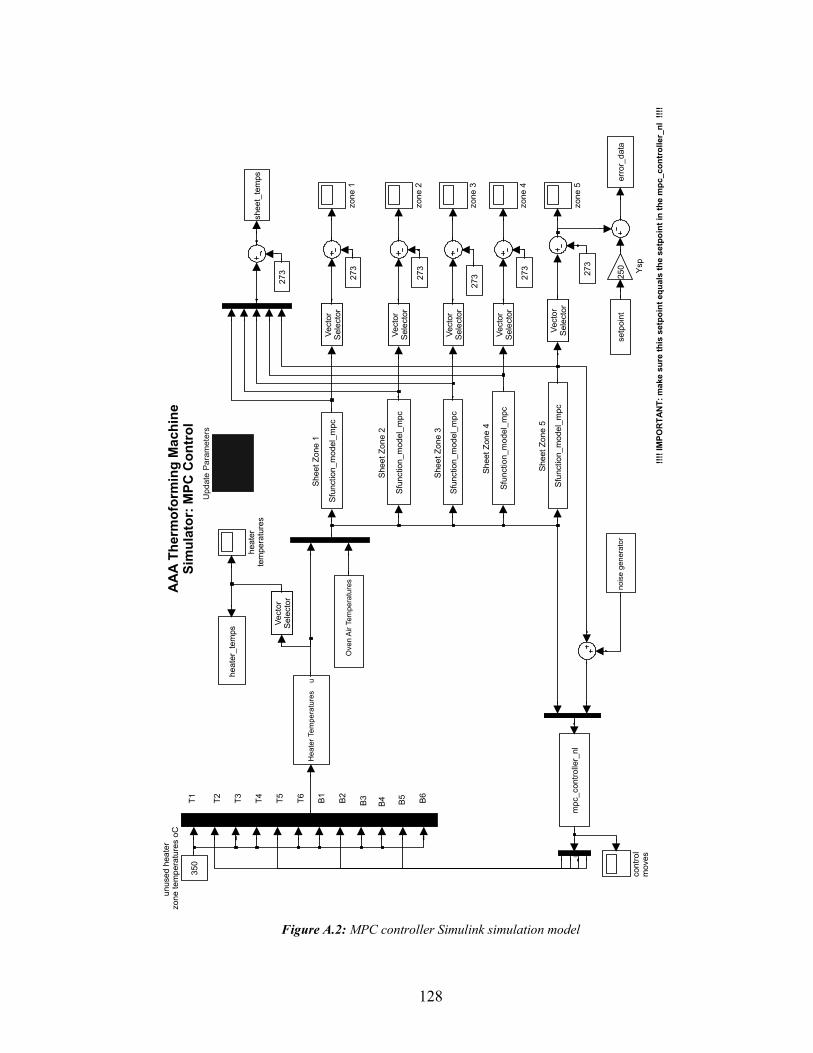
128
AA
A Th
erm
ofor
min
g M
achi
neSi
mul
ator
: MPC
Con
trol
T1 T2 T3 T4 T5 T6 B1 B2 B3 B4 B5 B6
!!!! I
MPO
RTA
NT:
mak
e su
re th
is s
etpo
int e
qual
s th
e se
tpoi
nt in
the
mpc
_con
trol
ler_
nl !
!!!
zone
5
zone
4
zone
3
zone
2
zone
1
350
unus
ed h
eate
r zo
ne te
mpe
ratu
res
oC
heat
erte
mpe
ratu
res
cont
rol
mov
es
250 Ys
p
? ?
?
Upd
ate
Para
met
ers
erro
r_da
ta
heat
er_t
emps
shee
t_te
mps
nois
e ge
nera
tor
Hea
ter T
empe
ratu
res
u
Ove
n Ai
r Tem
pera
ture
s
Sfun
ctio
n_m
odel
_mpc
Shee
t Zon
e 5
Sfun
ctio
n_m
odel
_mpc
Shee
t Zon
e 4
Sfun
ctio
n_m
odel
_mpc
Shee
t Zon
e 3
Sfun
ctio
n_m
odel
_mpc
Shee
t Zon
e 2
Sfun
ctio
n_m
odel
_mpc
Shee
t Zon
e 1
Vect
orSe
lect
or
Vect
orSe
lect
or
Vect
orSe
lect
or
Vect
orSe
lect
or
Vect
orSe
lect
or
Vect
orSe
lect
or
mpc
_con
trolle
r_nl
setp
oint
273 27
3
273
27327
3
273
Figure A.2: MPC controller Simulink simulation model
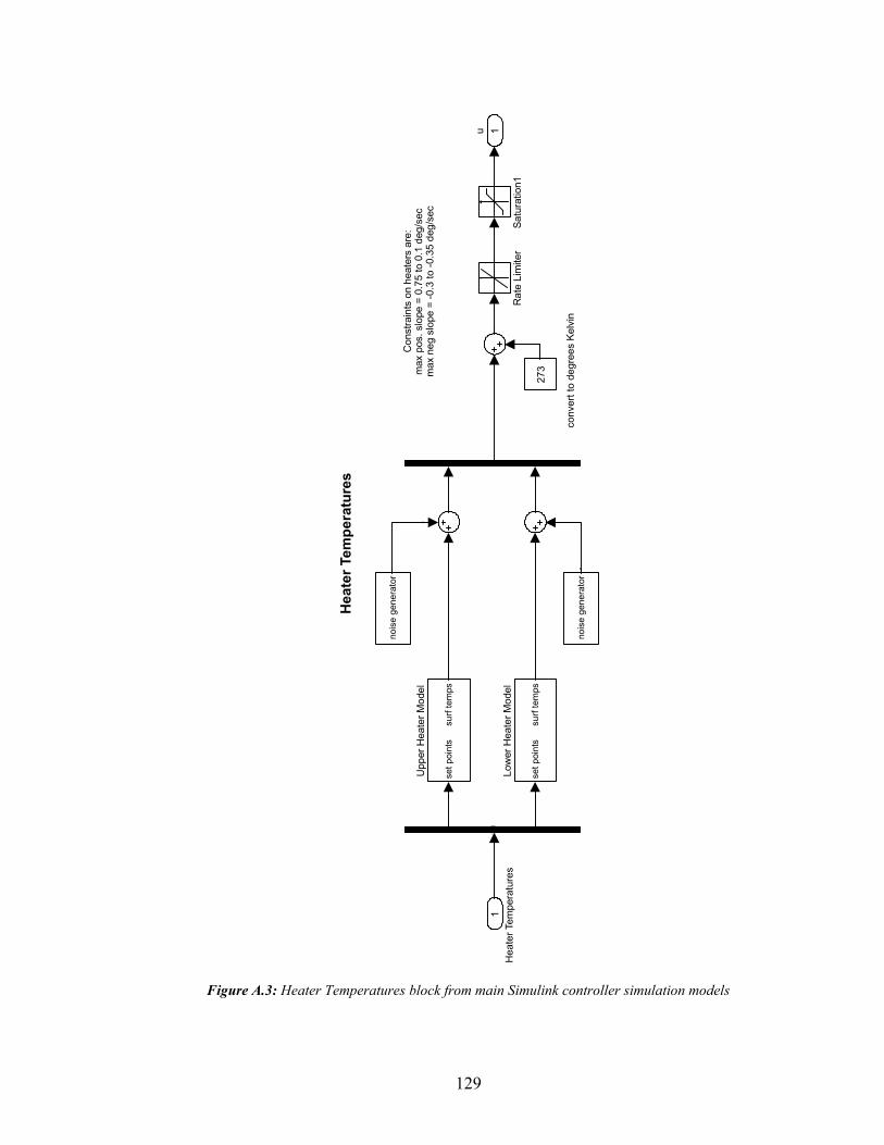
129
Figure A.3: Heater Temperatures block from main Simulink controller simulation models
conv
ert t
o de
gree
s Ke
lvin
Con
stra
ints
on
heat
ers
are:
max
pos
. slo
pe =
0.7
5 to
0.1
deg
/sec
max
neg
slo
pe =
-0.3
to -0
.35
deg/
sec
Hea
ter T
empe
ratu
res
1u
set p
oint
ssu
rf te
mps
Upp
er H
eate
r Mod
el
nois
e ge
nera
tor
nois
e ge
nera
tor
Satu
ratio
n1R
ate
Lim
iter
set p
oint
ssu
rf te
mps
Low
er H
eate
r Mod
el
273
1H
eate
r Tem
pera
ture
s
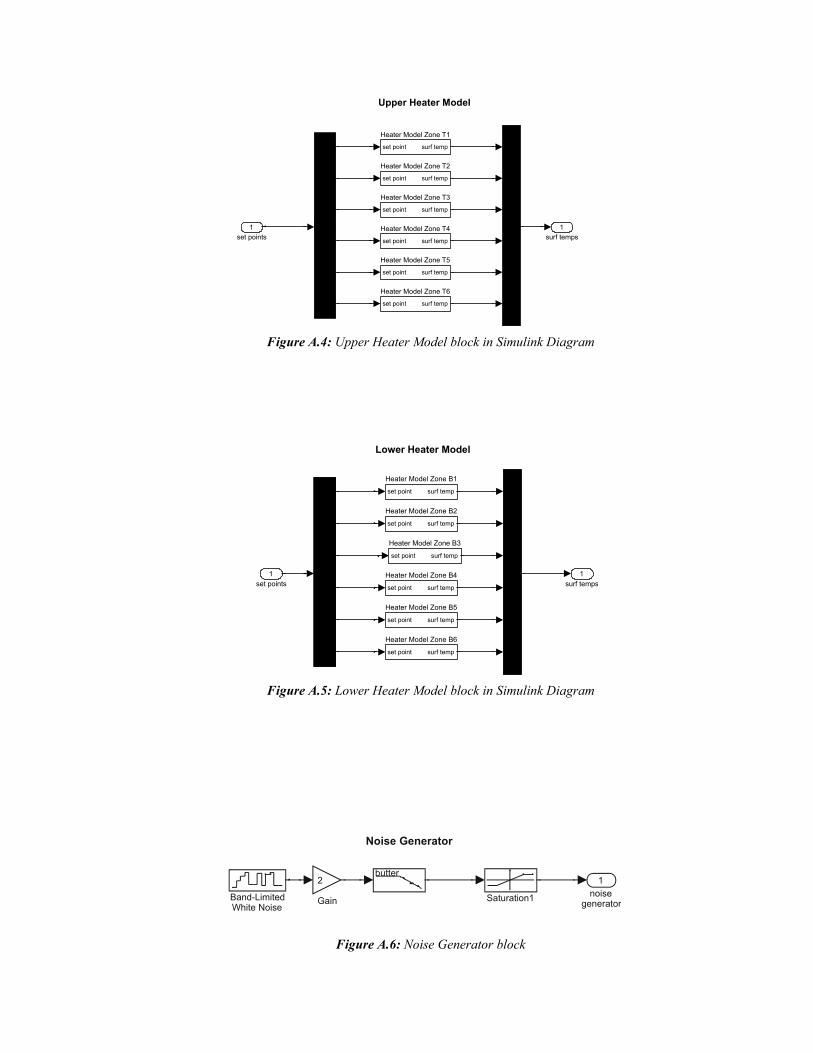
130
Upper Heater Model
1surf temps
set point surf temp
Heater Model Zone T6
set point surf temp
Heater Model Zone T5
set point surf temp
Heater Model Zone T4
set point surf temp
Heater Model Zone T3
set point surf temp
Heater Model Zone T2
set point surf temp
Heater Model Zone T1
Demux1set points
Noise Generator
1noise
generatorSaturation1
2
GainBand-LimitedWhite Noise
butter
Lower Heater Model
1surf temps
set point surf temp
Heater Model Zone B6
set point surf temp
Heater Model Zone B5
set point surf temp
Heater Model Zone B4
set point surf temp
Heater Model Zone B3
set point surf temp
Heater Model Zone B2
set point surf temp
Heater Model Zone B1
Demux1set points
Figure A.4: Upper Heater Model block in Simulink Diagram
Figure A.5: Lower Heater Model block in Simulink Diagram
Figure A.6: Noise Generator block
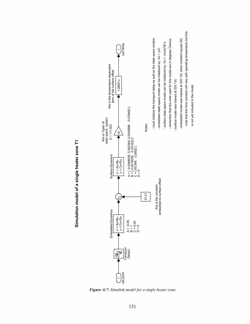
131
Sim
ulat
ion
mod
el o
f a s
ingl
e he
ater
zon
e T1
this
is 1
/gai
n of
st
ate
spac
e s
yste
mth
is is
the
tem
pera
ture
dep
enda
ntte
rm o
f the
sur
face
offs
et
Not
es:
- mus
t ini
tializ
e th
e tra
nspo
rt de
lay
as w
ell a
s th
e st
ate
spac
e m
odel
s
- em
bedd
ed s
tate
spa
ce m
odel
can
be
initi
aliz
ed b
y: X
o =
y/C
- rem
embe
r tha
t the
uni
ts u
sed
for t
his
mod
el a
re in
deg
rees
Cel
cius
- sur
face
mod
el w
as tr
aine
d at
325
^oC
- em
bedd
ed m
odel
was
trai
ned
at 3
25 ^
oC (t
ime
cons
tant
equ
als
20)
note
that
this
tim
e co
nsta
nt w
ill va
ry w
ith o
pera
ting
tem
pera
ture
but
this
is n
ot y
et in
clud
ed in
the
mod
el
- sur
face
sta
te s
pace
mod
el c
an b
e in
itial
ized
by:
Xo
= -in
v(A)
*B*u
K =
1/1.
023
this
is th
e co
nsta
nt
embe
dded
to s
urfa
ce o
ffset
A =
-0.0
5B
= 1
C =
0.0
5D
= 0
A =
[ -0.
0088
028
0.0
8236
4; 0
.004
5888
-0
.076
463
]B
= [ 0
.001
8038
-0
.001
622
]'C
= [
65.9
94
-2.6
602
]D
= 0
1su
rf te
mp
1.06
62*u
Tran
spor
tD
elay
2
x' =
Ax+
Bu y
= C
x+D
u
Surfa
ce D
ynam
ics
-K-
x' =
Ax+
Bu y
= C
x+D
u
Embe
dded
Dyn
amic
s
31.5
1
1se
t poi
nt
Figure A.7: Simulink model for a single heater zone
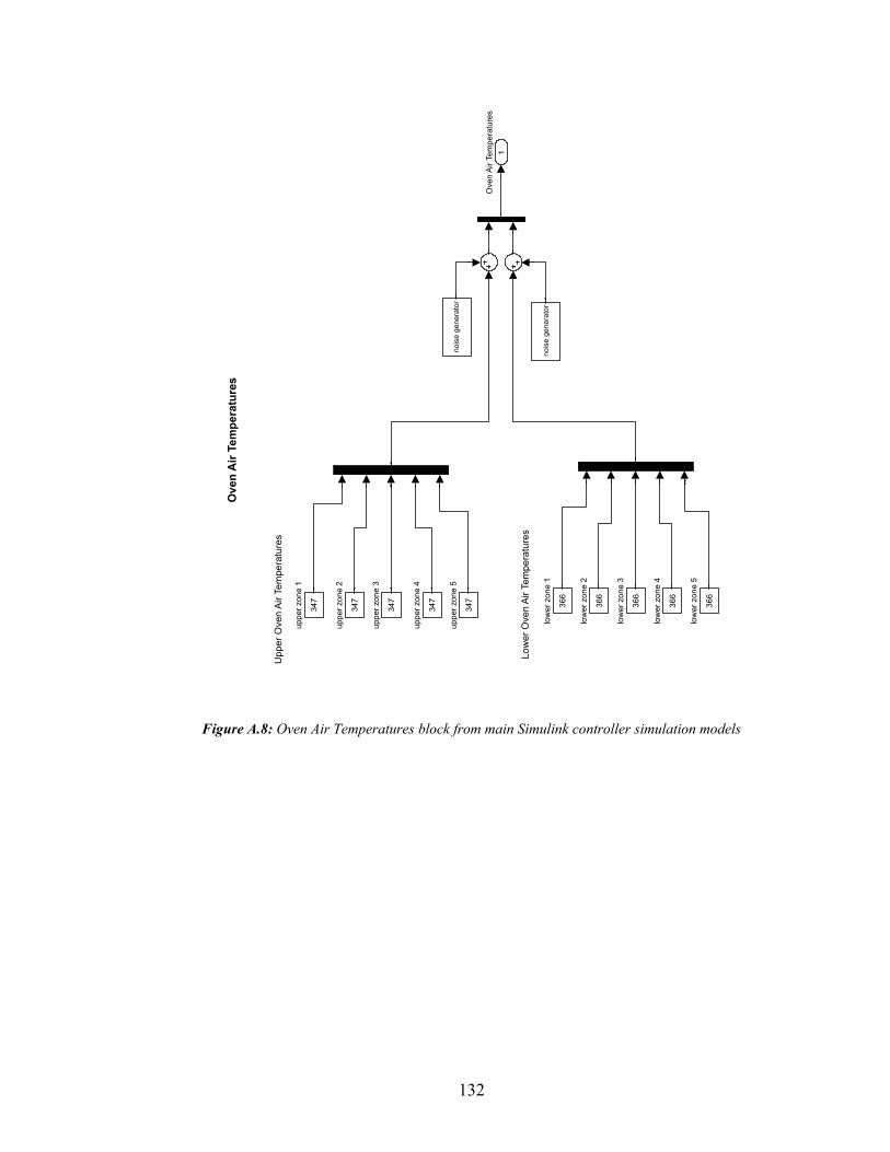
132
Upp
er O
ven
Air T
empe
ratu
res
Low
er O
ven
Air T
empe
ratu
res
Ove
n A
ir Te
mpe
ratu
res
1O
ven
Air T
empe
ratu
res
347
uppe
r zon
e 5
347
uppe
r zon
e 4
347
uppe
r zon
e 3
347
uppe
r zon
e 2
347
uppe
r zon
e 1
366
low
er z
one
5
366
low
er z
one
4
366
low
er z
one
3
366
low
er z
one
2
366
low
er z
one
1no
ise
gene
rato
r
nois
e ge
nera
tor
Figure A.8: Oven Air Temperatures block from main Simulink controller simulation models
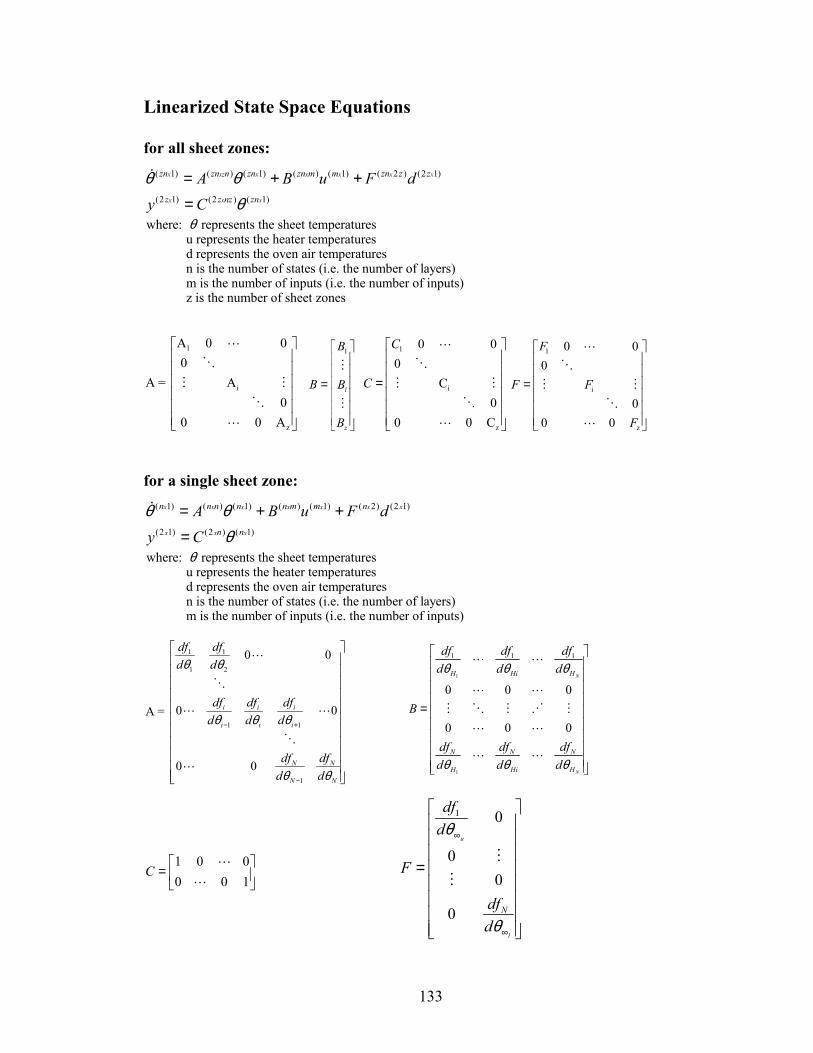
133
Linearized State Space Equations for all sheet zones:
( 1) ( ) ( 1) ( ) ( 1) ( 2 ) (2 1)
(2 1) (2 ) ( 1)
x xz x x x x x
x x x
zn zn n zn zn m m zn z z
z z nz zn
A B u F dy Cθ θ
θ= + +=
where: represents the sheet temperatures u represents the heater temperatures d represents the oven air temperatures n is the number of states (i.e. the number of l
θ
ayers) m is the number of inputs (i.e. the number of inputs) z is the number of sheet zones
1
i
z
A 0 00
A = A0
0 0 A
1
i
z
B
B B
B
=
1
i
z
0 00
C0
0 0 C
C
C
=
1
i
z
0 00
00 0
F
F F
F
=
for a single sheet zone: ( 1) ( ) ( 1) ( ) ( 1) ( 2) (2 1)
(2 1) (2 ) ( 1)
x x x x x x x
x x x
n n n n n m m n
n n
A B u F dy Cθ θ
θ= + +=
where: represents the sheet temperatures u represents the heater temperatures d represents the oven air temperatures n is the number of states (i.e. the number of l
θ
ayers) m is the number of inputs (i.e. the number of inputs)
1 1
1 2
1 1
1
0 0
0 0A =
0 0
i i i
i i i
N N
N N
df dfd d
df df dfd d d
df dfd d
θ θ
θ θ θ
θ θ
− +
−
1
1
1 1 1
0 0 0
0 0 0
N
N
H Hi H
N N N
H Hi H
df df dfd d d
B
df df dfd d d
θ θ θ
θ θ θ
=
1 0 00 0 1
C
=
1 0
00
0
u
l
N
dfd
F
dfd
θ
θ
∞
∞
=
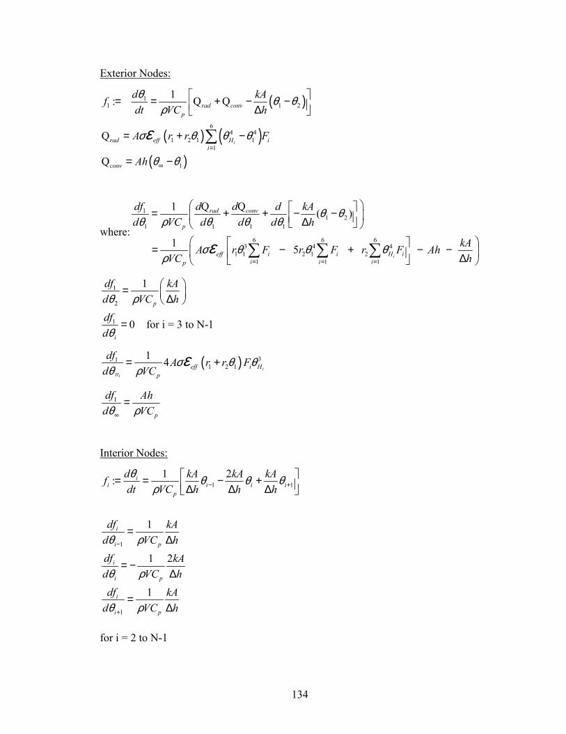
134
Exterior Nodes:
( )
( ) ( )( )
11 1 2
64 4
1 2 1 11
1
1: Q Q
Q
Q
i
rad convp
rad eff H ii
conv
d kAfdt VC h
A r r F
Ah
θ θ θρ
σ θ θ θ
θ θ
ε=
∞
= = + − − ∆
= + −
= −
∑
where:
11 2
1 1 1 1
6 6 63 4 4
1 1 2 1 21 1 1
Q Q1 ( )
1 5 i
rad conv
p
eff i i H ii i ip
d ddf d kAd VC d d d h
kAA r F r F r F AhVC h
θ θθ ρ θ θ θ
σ θ θ θρ
ε= = =
= + + − − ∆
= − + − − ∆ ∑ ∑ ∑
1
2
1
1
0 for i = 3 to N-1
p
i
df kAd VC hdfd
θ ρ
θ
= ∆
=
( ) 311 2 1
1 4i
Hi
eff i Hp
df A r r Fd VC
σ θ θθ ρ
ε= +
1
p
df Ahd VCθ ρ∞
=
Interior Nodes:
1 1
1
1
1 2:
1
1 2
1
ii i i i
p
i
i p
i
i p
i
i p
d kA kA kAfdt VC h h h
df kAd VC hdf kAd VC hdf kA
d VC h
θ θ θ θρ
θ ρ
θ ρ
θ ρ
− +
−
+
= = − + ∆ ∆ ∆
=∆
= −∆
=∆
for i = 2 to N-1