DYNAMIC ANALYSIS OF THE SOUTHERN AFRICA POWER POOL

(SAPP) NETWORK

SHAIBU ADAM IBU MLUDI

216073087

IN FULFILMENT OF MASTER OF SCIENCE DEGREE IN ELECTRICAL

ENGINEERING

COLLEGE OF AGRICULTURE, ENGINEERING AND SCIENCE

UNIVERSITY OF KWAZULU-NATAL

DECEMBER 2016

Supervisor: Prof. Innocent Ewean Davidson

ABSTRACT

Synchronous generators have been connected through overhead transmission lines and

interconnected to a regional power system network to improve reliability, enhance the security of

supply, trade electricity and share the available natural resources for energy fuel supply. The

interconnected power system experiences disturbances during normal operation such as load

variations and faults, causes stress on the generators to control and remain in synchronism. This

dissertation analyses the natural damping oscillations that will emanate during a disturbance in

the interconnected power system and provide understanding to the system operator to monitor

and operate effectively the Southern African Power Pool (SAPP). It is required to carry out the

performance analysis and characteristics of the generators during the disturbances in order to

identify the synchronizing and damping torque in respect of rotor angle and speed deviations. In

power system control, the frequency is monitored continually since the speed of the generators is

synchronized into the transmission lines. Any small variation on the interconnected system will

affect the others machines. The effect can either be the system maintaining its stability or loss of

synchronism. The latter can be avoided by identifying the nature and behaviour of oscillations

and determining effective means to minimize them in interconnected power pool. It can also

notify the system operator of an impending power outage. In this research investigation, a

simplified model of the Southern African Power Pool is modeled using DIgSILENT Powerfactory

power systems analysis software tool, using input data of the primary plant (synchronous

generators) and associated interconnected power system network. Nodal and modal analysis tools

were used to determine the dynamic status of the interconnected power network. A dynamic

analysis will enable participating members of the power pool understand the nature of oscillations

when affected by different types of events with continuous monitoring of the modes and

eventually assist in re-tuning of secondary control equipment to improve the service delivery of

electricity of a pool such as of the Southern African region.

The study has identified the focal points of power oscillations in the modelled SAPP grid through

simulations that affects the behaviour of system voltages during a disturbance and require to

control damping oscillations on the synchronous generators.

iii

COLLEGE OF AGRICULTURE, ENGINEERING AND SCIENCE

DECLARATION 1 - PLAGIARISM

I, ……………………………………….………………………., declare that

1. The research reported in this thesis, except where otherwise indicated, is my

original research.

2. This thesis has not been submitted for any degree or examination at any other

university.

3. This thesis does not contain other persons’ data, pictures, graphs or other

information, unless specifically acknowledged as being sourced from other persons.

4. This thesis does not contain other persons' writing, unless specifically

acknowledged as being sourced from other researchers. Where other written

sources have been quoted, then:

a. Their words have been re-written but the general information attributed to them has

been referenced

b. Where their exact words have been used, then their writing has been placed in italics

and inside quotation marks, and referenced.

5. This thesis does not contain text, graphics or tables copied and pasted from the

Internet, unless specifically acknowledged, and the source being detailed in the

thesis and in the References sections.

Signed……………………………………………………………………………

As the candidate’s supervisor, I agree to the submission of this thesis.

Signed: …………………………………………………………………………..

Professor Innocent E. Davidson

Form EX1-5

iv

TABLE OF CONTENTS

INTRODUCTION ................................................................................................................ 1

1.1 Overview of Southern Africa Power Pool ......................................................... 1

SAPP Network ............................................................................................ 2

1.2 Problem Formulation ......................................................................................... 3

1.3 Aims and Objectives .......................................................................................... 4

1.4 Motivation .......................................................................................................... 4

1.5 Hypothesis .......................................................................................................... 4

1.6 Research Questions ............................................................................................ 5

1.7 Methodology ...................................................................................................... 6

LITERATURE REVIEW ..................................................................................................... 7

2.1 Mechanical Energy on Synchronous Machines. ................................................ 9

Hydro Power Generation .......................................................................... 10

Thermal Power generation ........................................................................ 10

Torque on Synchronous Machine ............................................................. 12

Steady state of synchronous machine ....................................................... 12

Rotor Swing on two machines .................................................................. 15

Mechanical analysis of the synchronous machine .................................... 16

2.2 Primary plant of interconnected power system ................................................ 17

The synchronous generator ....................................................................... 17

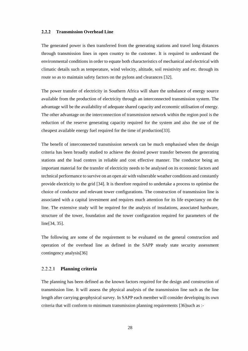
Transmission Overhead Line .................................................................... 28

Power transformers ................................................................................... 41

Power System Loads ................................................................................. 44

2.3 Simulation analysis of a single machine .......................................................... 47

Transient power analysis of power network ............................................. 50

Synchronous generators with controller ................................................... 55

Fault analysis in single line diagram ......................................................... 57

2.4 Damping oscillations in the overhead line ....................................................... 58

2.5 Calculations of parameters in synchronous generator ..................................... 60

Modal analysis for power system network ............................................... 63

MODELLING AND OPERATION OF SAPP GRID ........................................................ 66

3.1 Parameter for modelling in dynamic studies .................................................... 67

Direct energy transfer functions on generator .......................................... 67

Rotor equivalent electrical circuit ............................................................. 68

Determination of parameters for model .................................................... 72

3.2 Power system monitoring instruments ............................................................. 78

v

Input source of a transducers .................................................................... 79

Output signal of a transducer .................................................................... 79

Accuracy of transducers ............................................................................ 80

Energy Metering ....................................................................................... 86

Disturbance recorders ............................................................................... 87

3.3 Technical operations of SAPP Grid ................................................................. 88

Generation control .................................................................................... 88

SAPP GRID........................................................................................................................ 95

4.1 Modified SAPP Grid ........................................................................................ 97

Conditions for SAPP grid simulations ...................................................... 99

4.2 The dynamic controllers for SAPP grid ......................................................... 100

4.3 General governor requirements for Southern Africa ..................................... 101

4.4 Modelling of the governor for speed controller ............................................. 102

Hydro generation governor ..................................................................... 102

Hydro governor system model parameters ............................................. 107

4.5 Modelling of automatic voltage regulator ...................................................... 109

Types of excitation system [7, 8, 79] ...................................................... 109

SIMULATION OF RESULTS ......................................................................................... 114

5.1 Methodology and Simulation results of SAPP grid ....................................... 114

Rotor angle and frequency behaviour on synchronous generators ......... 114

Simulations of faults using electromagnetic transients of the turbine .... 119

Modal Analysis for SAPP grid ............................................................... 126

Methods to improve rotor speed in synchronous generators .................. 131

DISCUSSIONS ON THE DYNAMIC PERFORMANCE OF SAPP GRID ................... 132

6.1 Discussions on simulated results .................................................................... 133

CONCLUSIONS AND RECOMMENDATIONS ........................................................... 135

7.1 Recommendations .......................................................................................... 137

REFERENCES ................................................................................................................. 138

vi

LIST OF FIGURES

Figure 2-1: Illustration of a typical thermal power plant ...................................................................... 11 Figure 2-2: d and q axes for synchronous machine .............................................................................. 19 Figure 2-3: Simplified diagram of electrical circuits for d axis salient machines ................................... 21 Figure 2-4: Simplified diagram of electric circuits for q axis salient machines ...................................... 22 Figure 2-5: Open loop saturation for synchronous generator .............................................................. 25 Figure 2-6: Power angle characteristics of the excitation for the synchronous generator .................... 26 Figure 2-7: Saturation of synchronous generator during excitation ..................................................... 27 Figure 2-8: Representation of a single conductor with radius r ............................................................ 33 Figure 2-9: Symmetrical representation of a bundled conductor ......................................................... 35 Figure 2-10: Single line diagram for a single synchronous generator ................................................... 47 Figure 2-11: Results of simulated load flow for single machine ........................................................... 50 Figure 2-12: Simulation fault results of three phase fault on 400kV busbar ......................................... 51 Figure 2-13: Indicating oscillation of active and reactive power after disturbance .............................. 52 Figure 2-14: Rotor angle and speed behaviour after disturbance on busbar ........................................ 52 Figure 2-15: Single phase fault on Transmission line near the busbar .................................................. 53 Figure 2-16: Rotor angle and speed after fault at transmission line ..................................................... 54 Figure 2-17: Simulation results of single phase fault close to close busbar .......................................... 54 Figure 2-18: Simulation results of three phase fault on the transmission line ...................................... 55 Figure 2-19: Simulation results with voltage and speed controllers ..................................................... 56 Figure 2-20: Rotor angle and speed effects with controller ................................................................. 56 Figure 2-21: Illustration of stability plot in modal analysis ................................................................... 64 Figure 3-1: Rotor circuit as represented in DIgSILENT for d-axis ........................................................... 69 Figure 3-2: Rotor circuit as represented in DIgSILENT for q-axis ........................................................... 69 Figure 3-3: Growth of current in inductive circuits ............................................................................... 71 Figure 4-1: Typical power system diagram ........................................................................................... 97 Figure 4-2: SAPP diagram for dynamic analysis .................................................................................... 99 Figure 4-3: Functional block diagram for speed governor .................................................................. 102 Figure 4-4: Typical water parts for hydro plant .................................................................................. 103 Figure 4-5: Functional block for automatic voltage regulator ............................................................ 110 Figure 5-1: Frequency deviations after change of load in SAPP grid ................................................... 115 Figure 5-2: Rotor effects due to change of load in SAPP grid ............................................................. 115 Figure 5-3: Frequency deviations of a general fault on generator H1_6 ............................................. 116 Figure 5-4: Rotor angle effects of a general fault on H1_6 generator ................................................ 117 Figure 5-5: Frequency deviations of 3phase fault between T2_6 and Sub 31 ..................................... 118 Figure 5-6: Rotor effects due to 3phase fault between T2_6 and Sub 31 ........................................... 119 Figure 5-7: Frequency deviations of a 3phase fault between T1_6 and Sub 22 .................................. 120 Figure 5-8: Turbine power fluctuations due to a 3phase fault between T1_6 and Sub22 ................... 121 Figure 5-9: Frequency deviations of a 3phase fault between Sub 29 and sub 31 ................................ 122 Figure 5-10: Turbine power fluctuations due to a 3phase fault between Sub 29 and Sub 31 ............. 122 Figure 5-11: Voltage variations due to a 3 phase fault between Sub 29 and Sub 31 ........................... 123 Figure 5-12: Frequency deviations due to a fault between Sub 7 and Sub 8 ...................................... 124 Figure 5-13: Rotor angle effects due to a 3 phase fault between Sub 7 and Sub 8 ............................. 124 Figure 5-14: Voltage variations due to a fault between Sub 7 and Sub 8 ........................................... 125 Figure 5-15: Critical frequencies obtained for the modelled SAPP grid .............................................. 127 Figure 5-16: Controllability determined from mode 0001 .................................................................. 128 Figure 5-17: Observability determined from mode 0001 ................................................................... 129 Figure 5-18: Controllability determined from mode 002 .................................................................... 130 Figure 5-19: Observability determined from mode 0002 ................................................................... 130

vii

LIST OF TABLES

Table 3-1: Typical values of generator parameters .............................................................................. 76 Table 3-2: Operating Reserve for SAPP members in 2016 .................................................................... 93 Table 4-1: Required parameters for the speed governor ................................................................... 108 Table 5-1: Values for critical frequencies in the eigenvalue plot ........................................................ 126

viii

LIST OF ACRONYMS/ABBREVIATIONS

ABOM Agreement between Operating Members

AC Alternating Current ACE Area Control Error ACSR Aluminium Conductor Steel Reinforced

AGC Automatic Generation Control

AVR Automatic Voltage Regulator

CPS Control Performance Standards

DC Direct Current DIgSILENT DIgital SImuLation of Electrical NeTworks

DRC Democratic Republic of Congo

EAPP East Africa Power Pool

GCR Grid Code Requirement

GW,MW,W Units of Active power

Hz Hertz

IEEE Institute of Electrical and Electronic Engineers

IPP Independent Power Producer

kA, A units of current kJ/kg Units of carilofic values

kV Units of Voltage MCR Minimum Continuous Rating

mmf Magnetomotive force

MVA Units of apparent Power

MVAR units of reactive power

NERSA National Regulator of South Africa

NRS National Regulation Standard

SADC Southern Africa Development Community

SAPP Southern Africa Power Pool

SCADA Supervisory Control and Data Acquisition

UTC Universal Time Co-ordinated

WAPP West Africa Power Pool

1

CHAPTER 1

INTRODUCTION

1.1 Overview of Southern Africa Power Pool

In August 1995, Southern Africa Power Pool (SAPP) was formed as a regional electricity power

pool during the Southern Africa Development Community (SADC) summit that was held at

Kempton Park, South Africa by signing an Inter-Governmental Memorandum of Understanding

by member governments of SADC (excluding Mauritius)[1, 2] . On 23rd February 2006, a revised

Inter-Governmental Memorandum of Understanding was signed by Ministers responsible for

Energy in SADC[3]. The revised inter-Governmental Memorandum of Understanding was due to

the wind of change in the electricity sector reforms that has been restructured in SADC and

includes the introduction of electricity independent power producers.

There are twelve member countries in SAPP who are represented by the electric utility companies

in SADC with additional two members as Independent Power Producer and Independent

Transmission Company. The electric utility companies from Botswana, Mozambique, South

Africa, Lesotho, Namibia, Democratic Republic of Congo, Swaziland, Zambia and Zimbabwe are

Operating Members who are trading electricity power energy through the available market

practiced in SAPP. Three countries, namely: Malawi, Tanzania and Angola are termed non-

operating members [3, 4].

The operating members further signed other governing agreements that enable SAPP to sustain

equal participation for member utilities and thereafter provide reliable power system in the

interconnected electrical pool[2]. These are:-

a. Inter-Utility Memorandum of Understanding - This agreement serves as the fundamental

basis for management and operating principles of SAPP and also will uphold management

of the utilities to abide on the interconnection being organized by the member government.

This agreement will be signed by all member countries;

b. Agreement between Operating Members (ABOM)- This agreement is signed by only

operating members which has established the specific rules of operation and pricing.; and

c. Operating Guidelines which provide standards and operating guidelines that are used for

system planning and operation of the power system amongst member utilities.

Since the member utility companies were already operating their electricity networks before the

establishment of SAPP, therefore, the design, planning, and operations were based on each

2

country ‘s assessment and need. Moreover, the cross-border electricity trading existed in Zambia

and Zimbabwe, South Africa and Mozambique, and South Africa with Lesotho, Swaziland,

Botswana, and Namibia. The establishment of SAPP has facilitated the development of a

competitive electricity market in the SADC region such that non-operating members are engaged

in projects to extend transmission network and to upgrade into operating members in the pool [5].

Some operating members have increased their generation capacity and strengthened their

transmission networks.

SAPP Network

SAPP has an installed capacity of 61GW generated using power generation technologies, namely:

coal 62% from 38GW generated on thermal generation, hydro represents 21% from the total

generated 13GW , wind represents 4% of a total generation of 2.5GW, distillate 4% from various

different type of fuels such as ethanol, diesel and petrol driven generating machine and 2.7GW

the total generation, nuclear 3% and a total generation of 1.9GW, Solar PV represents 2.97% and

a total generation of 1.8GW , Open Cycle Gas Turbine has a total generation of 0.936 GW and

representing 1.51% , Solar concentrated solar panel 0.6GW and is representing 0.97GW and

remaining generation in the mix comes from landfill 0.002GW and Biomass 0,0042GW [2, 4].

The exploitation of these natural resources for the production of electric power requires careful

planning in order to optimize the use of these resources effectively and to obtain maximum

benefits at least cost, taking into consideration the need for minimal adverse environmental

impact.

SAPP Network is an interconnection of electric power supply networks from nine operating

members in the Southern Africa Region transmitting over long distances mostly in AC

transmission line and a DC link between Mozambique and South Africa at various voltage levels

from different types of generating plants[1]. There are two types of grid for the electricity trading

in the region, the first one can be termed as cross-border supply, the initial bilateral arrangements

before the inceptions of SAPP where electricity was traded from one country to the other such as

the South Africa and Mozambique at 533kV DC, 400kV and 132kV, South Africa and Swaziland

at 132kV, South Africa, and Lesotho 132kV transmission lines.

The second one can be termed as the interconnected electricity supply AC at 220kV and a 330kV

line running from the Democratic Republic of Congo running continuously through Zambia,

Zimbabwe, connecting at 400kV in Zimbabwe for Botswana up to South Africa. The second type

has been connected to mostly hydro generators. This implies that the SAPP network has a

complex mix and dynamics in its operation arising from different physical origins of electricity

3

production and a need to understand the natural response to disturbances when affected in the

interconnected grid.

The SAPP Network is operated by Control Coordination Centre to monitor the energy interchange

and electricity trading and the operating member has its own Area Control Centre for monitoring

and controlling the power system operation. The control centres will control the voltage and

frequency to achieve reliable and safe power system being traded in the region. The SAPP

Control Centre will only operate on the interconnected system that is required to be transferred

from one country to the other as per trading arrangement. The operation of the SAPP Control

Centre shall be to advise the operating member to control voltage and frequency being transferred

within the trading period and the rest of the utility responsibility.

1.2 Problem Formulation

The power system is extensively studied to assess its power flow and stability when subjected to

large disturbance. The assessment requires the data on the transmission line, transformer and

generator parameters to evaluate its impact on the system. However, customers also require the

usage of electricity through the connected transmission lines and the collective usage of the power

provides a profile to the total generation capacity of the network. SAPP power network

experiences disturbances on the interconnected system that take time to be explained by the

operating member states on the cause of such failure of power and affects the synchronized

generators. The Area Control Centres will visualize the sudden drop in frequency without the

option to avoid power failure. In some instances, protection relays have operated within the SAPP

network and affected another country but the later country will not realize the cause of fault that

affects transmission lines and synchronous generating machines.

A SAPP power system at its normal operating conditions is continually subjected to disturbances

and it is expected that the dynamic characteristics of the synchronous generators, transmission

lines will operate to control such disturbances to reinforce the system to remain in synchronism.

However, considering the available monitoring devices of SAPP interconnected power system, it

is very difficult to study and analyse system model based on assumptions of load and generated

power being constant for the system. In this research, it intends to investigate dynamic stability

of the SAPP network, and its impact on the behaviour of the generators when under the state of

disturbance basing on the available loading and generating power data. The research also intends

to provide further general knowledge of monitoring the power network on the interconnected

network on the impact when a disturbance has occurred in the system.

4

1.3 Aims and Objectives

The aim of the research study is to analyse simulations on the modelled grid from the four

participating SAPP members with interconnected power system. The grid simulation will be

conducted on the whole modelled SAPP grid and on the likely disturbance in the interconnected

system such as the faults on transmission lines and synchronous generators. In order to:-

a) Determine the effects of frequency relative to speed and rotor angle on its related

parameters on generating machine and transmission for SAPP network;

b) Analyse the simulated results and determine the magnitude of disturbances for SAPP

power system;

c) Determine the dynamic performances that should be required to be undertaken when

operating SAPP power system; and

d) Identify the available standards to be applied for system reliability indices for effective

operation of SAPP power system

1.4 Motivation

Presently the power networks worldwide are interconnected with other operating utilities and

depends on the use of system control to effectively utilize the available plants hence reliability

and value for money have become the source of electricity market reform and further expansion

of electricity development. This is the motivating factor that needs to be understood on how other

successful pools have operated their interconnected power system and their electricity supply

become free from unnecessary outages and disturbance. SAPP should be the mirrored to other

African power pools that operate the power pools with effective performance in the electricity

network.

Power system dynamic analysis is one of the studies required to be undertaken by SAPP region

in order to improve the controllability of the generating machines that are designed to produce at

least maximum power output so that it can withstand any sought of change whilst in synchronism.

This being the case, it will then provide a general behaviour in particular machines when an event

of disturbance has occurred to the system operator.

1.5 Hypothesis

The simulation of steady state stability will basically check power flow from a branch to the other

branch at normal operation and dynamic stability analysis will be simulated to check the effects

of disturbance on the system and the simulations will further compute the required generator

characteristic to determine the initial oscillation modes for the system where excitation and speed

5

governor are controlling the synchronous generators. This means that the power flow will be

determined by the capacity and loading of the network by using the Newton–Raphson algorithm

that converges the required solution for the large network and the eigenvectors for modified SAPP

grid.

Dynamic Analysis will, therefore, study the power system at generation plant that has been

subjected to small variations in load and generation at steady state conditions. It will further

analyse the effects of rotor angle due to insufficient synchronizing torque and also the behaviour

of rotor oscillations when there is insufficient damping torque[6]. SAPP network will be

represented in the single line diagram as the model in the DIgSILENT Powerfactory software

engineering tool in order to realize and understand the effects of small signal disturbance so that

sufficient damping torque is provided in the network.

The fundamental aspects of power stability will be based on the mathematical analysis of state

variable in the dynamic system that will derive the analytical techniques to encompass the power

system behaviour and pinpoint the other dynamics necessary for its operation by use of simulation

software[7].

1.6 Research Questions

There are a number of system disturbances reported every month in SAPP network. The root

cause will be investigated and analysed after following the sequence of events at a particular time

of the disturbance through the tripping of transmission and generation equipment. The post fault

analysis would be reduced when power system analysis could have included the effects of small

signal stability. Therefore, the research proposal seeks to answer the following research questions

during investigations:

a) What are the dynamic performance constraints apart from the transient studies that may

limit member countries from achieving the declared capacities for the SAPP network?

b) What strategic interventions are required in the SAPP network in order to perform

optimally at the desired operating conditions?

c) What are other most effective instrumentation/control tools and or strategies that can be

used to evaluate the dynamic performance in the SAPP Area Control Centres?

d) Using information obtained from the dynamic performance studies, how can the SAPP

network be optimally operated technically and economically using its operation guidelines

6

1.7 Methodology

The aim of the research study is to analyse effects of small disturbance in the interconnected

power system in particular with dynamics of generating machines and events of disturbance

caused by the transmission lines in SAPP Network

a) Literature Review on the fundamental principle of steady and transient state for multi

generating machines interconnected in a power pool.

b) Literature review on the theory and assessment of the small signal analysis and relate to the

simulated results. The literature review will assess SAPP Operating Guidelines;

c) Literature review to identify solutions for the system improvements on the grid networks

that will provide the improved delivery service for SAPP Network to reduce system

disturbances.

d) Develop single line diagram for the high voltage SAPP Network using in the Digital

Simulation of Electrical Network (DIgSILENT) Software;

e) Obtain data for the machines in generating stations, transmission lines and load that has

been connected in SAPP Network;

f) Run a simulation of the developed grid on SAPP Network;

g) Analyse the simulated waveforms and determine the magnitude of disturbances for SAPP

power system;

h) Determine the dynamic performances and place the required solutions to be undertaken to

improve efficiency when operating SAPP power system;

i) Identify the available standards to be applied for system reliability indices for effective

operation of the SAPP power system;

7

CHAPTER 2

LITERATURE REVIEW

Power system dynamic analysis can be described as the behaviour of the system between the

occurrence of a major disturbance and return to a steady state condition of a power network. It

encompasses the time the system is disturbed from a loaded condition through the disturbance to

the next action applied to the system equipment and controller to remain in synchronism. It

requires acquiring knowledge of characteristics and modelling of the individual system

component to determine the required dynamics of an interconnected power system[8]. However,

the dynamic analysis dwells on power system stability to operate and control energy balance in

order to provide sufficient restorative actions to counter disturbances.

Kundur et al[9]has defined power system stability in the Joint Task Force on Stability terms and

Definitions as: “the ability of an electric power system, for a given initial operating condition, to

regain a state of operating equilibrium after being subjected to a physical disturbance , with most

system variables bounded so that practically the entire system remains intact”. The definition

has termed the word ‘electric power system’ which comprises of the high voltage primary plant

and associated secondary equipment in the power network that will carry generated voltage and

the current drawn by end users. The primary plant equipment normally carries a potential charge

of the nominal rate of the voltage and secondary equipment provides a replica of the high voltage

and primary current flowing in the primary plant. The signal is used to provide an operational

status indication of the plant whether open or closed position.

The output values from the secondary equipment are used for indicating measuring instruments,

provide measured values for protection equipment and remote indications on the status of the

primary equipment in the substation. The primary plant in substations are adequately planned and

designed to perform their designed function but due to abnormal conditions, they will be subjected

to faults and change of load as the main physical disturbance, protection relays acquires the

measured values from the output of the secondary equipment to initiate and eliminate the

abnormal condition and also control abrupt change of parameters that has occurred in the primary

system.

The physical disturbance that has been stated in the definition can be stated to be the large

disturbance that has been studied extensively throughout the history of the power system. This

requires the protection system to detect, act and isolate the faulted part in the system either this

8

can be done immediately or time delayed depending on the magnitude of the fault or disturbance

that is caused by normal and sudden load changes. The physical disturbance depends on the

natural cause and should be able to be controlled by operating the affected part only and still

remain in synchronism. It is also important to understand that the synchronous generators

supplying the interconnected power system are also affected by such disturbance event[10].

The South African Grid Code has defined in its preamble that the interconnected power system

consists of the transmission network that can consist of the wire, electrical components connected

to the network. It also includes measurable components from the secondary equipment that

coordinate the operation to one power system in transmission level, generating station connected

to the national grid and international grid and the system operator[11]. Based on this definition

of an interconnected power system, dynamic stability analysis forms part of a vital study to

examine the damping oscillation of the synchronous machines that the measurable components

supporting the transmission network will not be able to indicate immediately the disturbance of

any nature. However, the damping oscillations of the power system require the understanding of

the characteristics of the generator design and its performance when affected by a disturbance in

the system. This is then required to analyse the behaviour of the generators when affected by the

disturbance system.

An interconnected network such as the Southern Africa Power Pool (SAPP) is made up of hydro-

based and coal-based generation sources for the extensive generation of electrical power to be

consumed and traded amongst operating members in SAPP. The design and size for the

hydropower stations are quite different from that of thermal stations. This investigation will study

and analyse the effects of damping oscillations in such a complex interconnected power system.

National electrical grids were established to serve each country .With regional integration, these

networks had to become interconnected to facilitate energy trading and maximising the economics

of scale, which an interconnected system have over non-interconnected disparate systems. In

Africa ,SAPP has low access to electricity of 24% if compared to 36% in East Africa power Pool

(EAPP) and 44% from West Africa Power Pool (WAPP) and this is due to a level mixture of

economies of member countries [12]. The low access of electricity in Southern Africa means that

average population of the Southern Africa Development Community (SADC) use different

sources of energy. South Africa has the highest electricity consumption and when even compared

to the rest of Africa and generates 62% of the total power in SAPP Pool[3]. The interconnection

of the grid is complex due to unilateral directional of power flow and the system is forced to

operate close to the maximum limit to suffice the market demand [13]. When a disturbance occurs,

the system misbehaves due to scattered location supplied with electricity, low electricity

consumption and also inadequate maintenance of power equipment [14].This then necessitates

9

the need to undertake different studies to suffice the growing demand for electricity in the

regional in order to reduce the public outburst when the quality of supply and services deteriorates

due to mitigation of system operation in the interconnected power system.

The generation of electricity will rotate synchronous machines and physical movement of the

equipment will be required for massive mechanical machinery to produce electricity that will be

synchronised into the network. The analogy is the conversion of systems from mechanical to

electrical energy and turns to be electrical to mechanical energy when under any disturbance

.Therefore, another complexity arises when multi-machines supply the interconnected power

system, when a disturbance occurs the electromechanical oscillations will change its phenomena

and synchronism might be disturbed in the power system [15].The occurrence of unstable

oscillations have been known through various tests on 132 kV line with a single generator and

also through a various study on mathematical derivations [16].The recent study occurred in an

interconnected power pool where a heavily loaded transmission line feeder circuit breaker failed

to eliminate a fault causing the source of supply breaker to isolate the fault and caused a total

shutdown of the network . An investigation that was carried out revealed that automatic

generation control equipment tried to restore supply as per operation condition of load dispatch

but the load stress caused other lines to trip and limited reactive power from the generators that

were producing a low capacity of power[17] . The investigation revealed the system outage was

caused by damping oscillations on the network after carrying out modelling and simulation of the

system network.

The main power generations in the Southern Africa are based on the water and coal as the main

source of energy. Most of the hydro generations in Zambia, Zimbabwe, DRC and Mozambique

has its supplied been consumed in South Africa and South Africa has its main supply from thermal

and other sources of energy. Most countries have resolved to accelerate new development of

generation plants and its evacuation power in the countries where available natural resources can

sufficiently make an impact in the incremental of access of safe and reliable electricity supply.

The essence of high level studies is essential to be undertaken to improve dynamic modelling on

the new plant and the old plant to verify the power plant dynamic data that is required in most

utilities in the Southern Africa so that will determine the different characteristics and behaviour

of different equipment connected to the system under any type disturbance [13]

2.1 Mechanical Energy on Synchronous Machines.

The fundamental relationships and mathematical equations of the synchronous machine are as

follows:

10

Hydro Power Generation

In hydro-electric power generation, energy conversion takes place in accordance with the Law of

Conservation of Energy, from water falling from a height (potential energy) and impinging on

turbine blades to initiate rotation (kinetic energy).

Countries that have suitable hydro generation potentials, such as Zambia, Democratic Republic

of Congo, Zimbabwe, have sites, which are developed after feasibility studies are conducted to

ascertain the technical, economic, environmental and Social impact assessment[18] has been

fulfilled with mitigating factors. Therefore generating capacity on hydro-electrical power will be

a function of constant flow rate of the perennial river or into the storage and head to discharge

hydraulic turbines basic equation for the hydropower generation is stated as follows[19]:

P=9.81 η ρ Q H (2.1)

Where:

P = Power

η= Plant efficiency

Q= Discharge flow rate (m3/s)

H= head (m)

ρ = density of water (kg/m3)

Thermal Power generation

In an interconnected power utility such as SAPP, the natural resources to produce electricity will

indirectly assist countries with trade cooperation and just like in Southern Africa, South Africa

has abundant coal deposits about 53 billion tonnes and it will take ages to be depleted hence large

generation of electrical power is guaranteed for the country [20] and the region.

Thermal generation plant referred in figure (2.1) is installed close to the site where coal is

extracted or where there are an ease means of transportation to the generation station. The coal

particles are crushed into dust in the pulverising mill in order to increase the surface area and

aeration in the boiler. The pulverised coal is combusted and burn in the boiler to heat water to

produce high-temperature high-pressure steam which is used to generate electricity by the

turbines. The steam is also absorbed, condensed and reformed into water, ready to be recycled for

11

the production of steam in the boiler. The temperature of the recycled water going into the boiler

through the cyclone needs to be almost the same degrees with the already available water in the

boiler.

Crushed coal is fed mechanically or pneumatically to the lower portion of the boiler as shown in

figure 2-1. The forced draft fan will blow air at the bottom of the boiler so that air will be used

to constantly burn the crushed coal. Steam and dust will leave the boiler. Fuel gas treatment will

be initiated from the boiler and undergoes into processing cycles in the cyclone where dust is

separated and fall into the dust collector. The induced draft fan will the used to release gas into

air after being purified in the stack. From the dust collector, dust is recycled at the back of the

boiler to provide uniform low portion of temperature. The dust collector also captures sulphur

that further provides combustion efficiency through heat absorption in the walls of the boiler.

Flue gas leaving the cyclones passes through the dust collector and induced-draft fan to the stack.

Dust inventory in the boiler is controlled by draining hot ashes through an ash cooler. In the

gasification process, coal is partially reacted with a deficiency of air to produce low heating value

fuel gas.

Therefore, the thermal generation requires the quantification of coal with good calorific values

kJ/kg, availability of water and transport to constantly supply the generating plants. The thermal

generation plant relies on the heat to drive mechanical equipment for the production electricity.

Figure 2-1: Illustration of a typical thermal power plant

12

Torque on Synchronous Machine

When a source of energy has been initiated to start flowing into the generation system, whether

hydro or thermal, it will then turn the massive mechanical equipment by rotating the rotor and

generate electricity through the stator windings. The generated voltage will be transformed at

different levels before being consumed by the end user and mostly located at very long distance

away from the generation plant.

When the generation system and its associated supply are synchronised into the grid, then the

system is operating at normal conditions, it will be termed as steady state. However, when the

steady state is disturbed, distorted torques will act on the rotor and the net torque will then the

change speed to either accelerate or decelerate[21]as defined below.

Where:

aT = accelerating torque ( mN . )

mT = driving mechanical torque ( mN . )

eT = load electrical torque ( mN . )

From the equation (2.2), when the system is in the steady state then em TT , because the torque

from the turbine and rotor shaft is synchronised with the corresponding voltage produced in the

stator and load with constant synchronous speed, s

Steady state of synchronous machine

In all type of generations, the energy source will drive a massive equipment for it to convert from

heat or kinetic energy into mechanical energy through turbines and rotor through the stator

windings to generate a symmetrical electrical voltage. Therefore, the stability of machines will be

determined by angular momentum and inertia constant of synchronous generators because it is

related to laws of motion. The inertia constant, H, denotes the kinetic energy stored in the rotating

parts of the machine at synchronous speed per unit rating of the machine in G MVA

T𝑎 = 𝑇𝑚 − 𝑇𝑒 (2-1)

𝐺𝐻 =

1

2𝐽𝜔2

(2.2)

13

Where:

J = polar moment of inertia of the generating parts (Kg/m2)

s = angular synchronous velocity in electrical radians/s and

= 360f electrical degrees per second

If M is the corresponding angular momentum, then

M = Jωs

Where:

f = system frequency in Hertz.

The momentum of the machine, when disturbed, should have an impact on oscillation before such

mass of the equipment will halt to a standstill also the weight of the rotating machine shall not

stop immediately and hence will obey the laws of motion. The moment of inertia of synchronous

generator is given

𝑀 =

𝑊𝑅2

32.2 𝑙𝑏. 𝑓2

(2.4)

Where:

W = weight of the rotating parts of the machine and

R = radius of gyration but the manufacturer of the machine will only provide the value of

WR2.

From equation (2-1), where em TT then to obtain power, torque is multiplied by synchronous

speed, s

𝑇𝑚𝜔𝑠 − 𝑇𝑒𝜔𝑠 = 𝑃𝑚 − 𝑃𝑒 = 0 (2.5)

Where:

𝑀 =𝐺𝐻

180f (2.3)

14

𝑃𝑚 = represents mechanical Power

𝑃𝑒 = represents electrical Power

When electrical power, eP changes, it means that the loading of the generator has changed and

mechanical torque, mP should be maintained to remain constant after the synchronous speed

changed.

The motion of the rotor is then described by second order equation and obeys newton second law

of motion. Hence, the equation of motion shall correspond to the total change of power as shown:-

Pa = Pm − Pe = M

d2θ

dt2

(2.6)

but now aP shall be the total power generated by the machine and will represent the angular

position of the rotor in the stator winding and when in steady state it will be 𝑑𝜃

𝑑𝑡 equal to

synchronous speed, so t where the constant 𝜹 is called the power angle of the

synchronous machine. If it is then substituted with equation (2.6), by combining with equation

(2.3),f

GHM

180 and divide by G in the same equation (2.3), per unit of the machine is obtained

and will be as provided in the below equation: -

𝐻

180𝑓

𝑑2𝛿

𝑑𝑡2= 𝑃𝑚 − 𝑃𝑒 = 𝑃𝑎

(2.7)

Where:

H = Inertia constant of the machine

f180 = nominal speed = ( f2 ) radian/s

2

2

dt

d = changes of load angle

The equation ((2.7) is the fundamental swing equation and states the required parameters

necessary for dynamics and stability on steady state of the machine but has been realised without

assuming the reality on variation of load and the following : -

15

Assumption 1: Angular momentum is taken as constant as 1.11x 10-4H, and

Assumption 2: Damping 𝑑𝛿

𝑑𝑡 has been neglected with the thinking of adequacy

amplitude attained on the so called first swing and the system will be

able to eliminate the disturbance and remain in synchronism.

Rotor Swing on two machines

From equation (2.6), where2

2

dt

dMPPP ema

, it is can be expressed the same for each

machine

𝑀1

𝑑2𝛿1

𝑑𝑡2= 𝑃𝑚1 − 𝑃𝑒1

(2.8)

𝑀2

𝑑2𝛿2

𝑑𝑡2= 𝑃𝑚2 − 𝑃𝑒2

(2.9)

Where:

1 and 2 are integers for 𝑀1 , 𝑀2, 𝛿1, 𝛿2, 𝑃𝑚1, 𝑃𝑚2, 𝑃𝑒1 𝑎𝑛𝑑 𝑃𝑒2

Let the power angle between two rotor axes from two separate machines but at the same

generating station be 𝛿 = 𝛿1 − 𝛿2and when the equations (2.8) and (2.9) are combined, it will

simplify the calculation, the result will be as follows:

𝑀

𝑑2𝛿

𝑑𝑡2= 𝑃𝑚 − 𝑃𝑒

(2.10)

Where:

𝑀 =M1M2

M1+M2

𝑃𝑚 =

𝑀2𝑃𝑚1 − 𝑀1𝑃𝑚2

𝑀1 + 𝑀2

(2.11a)

𝑃𝑒 =

𝑀2𝑃𝑒1 − 𝑀1𝑃𝑒2

𝑀1 + 𝑀2

(2.11b)

16

The result of the rotor swing on two-machine has the same effect as a connection of resistances

in a parallel circuit and being at the same station, the rotor angular momentum will be almost the

same values and in most of the cases, it will be manufactured by one company.

Mechanical analysis of the synchronous machine

From the explanation on rotor dynamics, it has been observed that damping and kinetic

acceleration have been neglected and dealt only with a steady state operation where at any slow

change in the system the kinetic energy remains unchanged.

If a three phase fault is then considered, the worst scenario, where all voltages will be zero and

consequently lose the load, the machine load will be reduced to zero and with a good protection

system, the generator will be spinning getting ready to be synchronised into the system. When

such moments occur then, the general energy equation should be considered where mechanical

energy = electrical energy ± kinetic energy + losses.

From equation (2.6), where aem PPP

dt

dM

2

2 , is loaded synchronised machine and since

the mechanical power will be constant, but when a fault occurs then the equation will be

represented as follows

𝑀

𝑑2𝛿

𝑑𝑡2+ 𝐾

𝑑𝛿

𝑑𝑡+ 𝑃𝑒 sin 𝛿 = 𝑃𝑚

(2.11)

Where:

M = angular momentum

𝐾𝑑𝛿

𝑑𝑡 = damping velocity

𝑃𝑒 sin 𝛿 = electrical power

Pm = mechanical power

When a disturbance has occurred in the system, 𝐾𝑑𝛿

𝑑𝑡 will tend to accelerate and then decelerate

before it settles down; and electrical power, 𝑃𝑒 sin 𝛿 will be equal to zero.

17

2.2 Primary plant of interconnected power system

The following primary equipment represents the electrical circuits with its characteristics and

behaviour that are used in the interconnected power system. These equipment have been used for

the study of dynamic analysis in the DIgSILENT Powerfactory software tool and will be

examined as the transient behaviour of power pool.

The synchronous generator

The synchronous machine for ac generator is driven by a turbine coupled with rotor and rotor

shaft to change the exerted mechanical energy into electrical energy. The electrical energy will

be produced by the rotation of the rotor shaft coupled with field windings that will eventually

generate the resultant magnetomotive force (mmf) with the stationary stator windings.

The field windings will be excited by being injected with a separate source current for the

production of the magnetic field which will thereafter induce alternating voltages in the armature

windings of the generator[22]. However, the high magnetomotive force that the separate source

current will initiate when combined with the current in the armature windings, the resultant flux

across the air gap between the rotor and generator generates voltage in the coils of the armature

windings and provides the electromagnetic torque between stator and rotor.

It is important to note that the armature windings carry the electrical load for the grid and also

operate at higher voltage than field windings hence will be subjected to sudden changes of load

and faults hence requires mechanical strength and insulation.

The interconnected power pools such as SAPP will contribute to the pool with generators such as

thermal and hydro types of generators that are connected to the grid. They difference of the

generator arises from the type of energy sources being used for the generation of electricity and

as such thermal and hydro have a different type of the rotor pole arrangements such as round and

salient pole rotor respectively.

Armature reaction with the field windings

The armature windings are spaced and distributed at 120°electrical degrees apart to allow equal

rotation of magnetic field by the rotor and thereafter voltage which has been placed at

120°electrical degrees will be produced in the windings with a constant time phase.

The rotation of the rotor at constant speed ωs will produce the magnetic field for the electrical

energy that will undulate with the changes of its position relative to the design of the stator

18

windings. At any moment when the machine is rotating magnetomotive force (mmf) is produced

through the air gap designed in between the stator and rotor and due to the electromotive force

from the field windings and the total mmf will have a sinusoidal spatial distribution with constant

amplitude and phase angle ωst as the function of time[7]. The whole sinusoidal wave will then

move at a constant velocity of ωs, electrical rad/s.

For the machine with Pf field poles, the speed of rotation of the stator field is

Where:

ωsm = synchronous machine speed

Pf = field Poles of the machine

ωs =Synchronous speed in radians per sec

𝑓 = system frequency

𝜂𝑠 = Speed in revs per sec

This the same as the synchronous speed, ωs of the rotor in equation (2.2),

𝐺𝐻 =1

2𝐽𝜔𝑠

2 that has been represented 𝝎 as for the swings of the machine.

Electrical Equivalents for Synchronous Machines using Direct and Quadrature

Axes

Figure 2-2, depicts the synchronous machine with a salient rotor and the phases of the generator

terminal lie in the stator windings on a- axis, b-axis and c- axis where the windings a, b, and c

respectively represents points that will be connected to the grid.

The field windings are represented by the windings labelled, e on d-axis and supplied through ve

and the windings Q and D on q- axis and extended d- axis represents the damping windings[23]

ωsm =

2

Pfωs mech. rad s⁄

𝜂𝑠 =

60𝜔𝑠𝑚

2𝜋=

120𝑓

𝑃𝑓 𝑟𝑒𝑣𝑠 𝑚𝑖𝑛⁄

(2.12)

19

The d and q axes for synchronous machine can be analysed by self-inductances and the linear flux

-mmf relationship for each coil in the a ,b and c axes to be aL , bL and cL be equal to each

other and mutual inductance due to magnetically coupled windings Lab, Lbc and Lca in between

each adjacent pair of concentrated coils[24] of the same axes.

In accordance with Faraday’s Law[7], the self-induced voltage in respect of the instantaneous

value of flux linkage, ψ, as such saturation and hysteresis of the magnetic circuit and eddy current

in the armature is not considered. It considered in that manner so that the distribution of flux in

the stator winding is systematically sinusoidal [25]. Where flux, = 𝐿𝑖 , the n the following is

derived

𝑢𝑎 =

𝑑𝜓𝑖

𝑑𝑡+ 𝑟𝑎

(2.13)

Where:

ar = resistor connected in series and,

i = current

au = induced voltage

Figure 2-: d and q axes for synchronous machine

Figure 2-2: d and q axes for synchronous machine

20

t = time in electrical radians

On similar note the two magnetically coupled windings between coils a and b, the induced voltage

will be derived as below

ua =

dψ1

dt+ rai1

𝑢𝑏 =

𝑑𝜓2

𝑑𝑡+ 𝑟𝑏𝑖2

(2.14)

Where:

ba rr , = resistor connected in series

21, ii = instantaneous current between coils in the phases

ba uu , = induced voltage between the coil in the phases

21, = flux in the phases

The self and mutual inductances of the stator circuits will change with the rotor position due to

variations of permeance of magnet flux path caused by non-uniform air gap from the field

windings hence the voltage for the stator circuit will be represented as below[7, 26]:

ua =

dψa

dt− Raia = ηψa − Raia

ub = nψb − Raib

𝑢𝑐 = 𝜂𝜓𝑐 − 𝑅𝑎𝑖𝑐 (2.15)

Where

cba uuu ,, = induced voltage in stator windings

cba ,, = flux in the phases between stator and rotor

aR = Stator winding resistance

cba iii ,, = current flow in the stator windings

21

= represents the differentialdt

d

The common study of salient pole synchronous machine has been solved in terms of rotor with

two axes of mechanical rectangular symmetry [27]called

a) Direct (d) axis are centred magnetically in the centre of north pole

b) Quadrature (q) axis, positioned 90° electrical ahead of the d axis

Various studies have shown that dq0 transformation suits very well when the synchronous

generator has three phase balanced reactance and armature resistance in the machine. With this

concept of a balanced circuit for the rotor and stator then disturbance of any sought will be solved

by the circuit representation of dq0 transformation by equation (2.16) whether it's capacitive or

inductive load[26, 28].

Figure 2-3 and 2-4 represents the simplified diagram for synchronous machines for d and q axis

that has been adopted by IEEE standard definition [27, 29] to represent electrical circuit diagram

of d and q axes based on the leakage and mutual reactance.

Figure 2-3: Simplified diagram of electrical circuits for d axis salient machines

22

Where:

dq , : Total flux linkage with respect to efficiency of speed

qd ii , : Current flow in the d and q axes respectively

lX : Stator leakage Reactance

sR : Stator resistance in Ohms

rlX : Armature leakage between field and damper winding

mdX : Mutual reactance between field and damping windings on d axis

mqX : Mutual reactance between field and damping windings on q axis

QD XX , : Damping reactance in extended d axis

eX : Mutual reactance between damping and field windings

QD RR , : Equivalent damping resistance

DQ ii , : Instantaneous d- and q axis damper winding current

Figure 2-4: Simplified diagram of electric circuits for q axis salient machines

23

Basically, the equivalent phase voltages on d and q axes for the stator in terms of phase flux

linkages and currents from equation (2.15) by applying dq0 transformation will result in

transformed components of voltages, flux linkages and currents as follow [7]:

Where:

0,, eee dq = transient voltages in dq0 axis in respect to stator windings

,, dq = flux in the phases between dq axis

aR = Stator winding resistance

0,, iii qd = current flow in the in the dq0 axis

p = the differential operatordt

d

= phase angle between a-axis and d-axis (figure 2-2)

p = angular velocity of the rotor

= f 2 electrical rad/s

From equation (2.16), pq and pd show that flux and change of load angle has a common

reference point to generate voltages on the other side on d and q axes and rotates in synchronism

with the stationary armature coil. The terms also denote the change of flux dp and qp due

to space between the rotor and stator (speed voltages) which will change due to frequency from

the grid in terms of the voltage measured from the grid transformer.

𝑒𝑑= p𝜓𝑑– 𝜓𝑑𝑝𝜃 − 𝑅𝑎𝑖𝑑

𝑒𝑞= p𝜓𝑞 − 𝜓𝑞𝑝𝜃 − 𝑅𝑎𝑖𝑞

𝑒0 = p𝜓0 – 𝑅𝑎𝑖0 (2.16)

24

When 0,, iii qd remains constant as the rotor moves then there will be no change to the stored

magnetic energy. The rotor power output will be equal in magnitude and opposite in the sign to

the rotor losses as has been shown in equation (2.11) and has been derived from where mechanical

energy = electrical energy ± kinetic energy + losses

𝑀𝑑2𝛿

𝑑𝑡2+ 𝐾

𝑑𝛿

𝑑𝑡+ 𝑃𝑒 sin 𝛿 = 𝑃𝑚

Where

2

2

dt

dM

= kinetic energy across the gap

𝐾𝑑𝛿

𝑑𝑡 = rate of decrease of total stored energy

𝑃𝑒 sin 𝛿 = electrical energy

Pm = Mechanical power

Saturation of mutual reactance of synchronous machines

The production of electricity is due to a magnetic force caused by rotation of the rotor to the

windings of the stator. Principally, the flux density is proportional to magnetic field strength and

until such a time it become saturated due to the material used for the permeance of flux and mostly

iron is used for the windings the synchronous machine.

Therefore, the magnetic strength of the electromagnetic depends on the number of turns of the

coil, current flowing through the coil or the type of material being used and then identify the

maximum current that will require protecting the generator windings.

Generally, saturation effects are not considered when it's assumed to operate within the steady

state value. In the winding circuits where reactance will be used to change into another measurand,

saturation will exist in the reactance of synchronous machines. However, it will be proper to

include the saturation of magnetising circuits in the reactance between axis and dq axes as aqx

and adx . Figure 2-5 presents the saturation of the synchronous generator between the terminal

voltage on y-axis and excitation current on x-axis.

25

The air gap line indicates the excitation current that is needed to overcome the reluctance of the

air gap and to remain constant at an increase of voltage and current. The degree of saturation can

be noted when the air-gap line departs with the open circuit characteristic curve. The values are

given under open circuit conditions so that U1.0 is actually behind xl the leakage reactance and

saturated magnetising inductance Xrl. The generation saturation SG shall be used as the basis of

saturation functions [8].

Saturation of self-inductance on rotor circuit due to voltage regulation

It has been stated that field windings will be excited by being injected with a separate source

current and thereafter induce alternating voltages in the armature windings of the generator. It is

the excitation that will be used to regulate the generated voltage to prevent the saturation of the

generator. However, in an event of any disturbances, if the change of voltage is within its dead

band and has not reached the maximum or minimum voltage shall not change to the new voltage

level and even if the settings can be changed to the minimum set[30].

Figure 2-5: Open loop saturation for synchronous generator

26

In figure 2-6 indicates the characteristics of the power angle curve on the behaviour of excitation

voltage at increased power. Considered the rated generator voltage and varied the exciter voltage.

The shapes were achieved with beyond rated saturation in figure 2-6.

Figure 2-6 was obtained on the test that was carried on voltage regulator that was controlling

excitation voltage by assisting or opposing the current flow in order to maintain the generator

voltage preferably constant [31]. The figure shows an inversely proportional to power generated

with the load angle at the terminal of the generator. Shape 1 presents that the machine is under

excited at about 50% of the load with an increasing mode and corresponds to the air gap line.

Shape 2 indicates the normal excitation at 100% load but will hold down voltages at full load.

Shape 3 indicates that over excitation of generation.

Figure 2-7 was obtained by the simulation of the single generator. The generator was simulated

with a fault that took a long time before being cleared and the result on the power angle has the

three shapes that were done by actual test.

Figure 2-6: Power angle characteristics of the excitation for the synchronous generator

27

Figure 2-7 was obtained during the simulation on DIgSILENT Powerfactory software tool on a

single short circuit fault near the generation station and the results of the power angle are

generated as the mode of shapes. However, it can be noted that during the fault, the exciter will

be regulating the voltages of the faulted generator. This gives the advantage to understand that

the generator will undergo the different processing of excitation as shown as shapes in figure 2-

7.The plot of figure 2- 7 has been labelled under excitation as in shape 1 of figure 2-6, normal as

in shape 2 in figure 2-6 and over excitation for the shape of 3 in figure 2-6.

Figure 2-6 was produced at every instant value to measure the power–angle diagram but the

approximation on the plot has been adequately detailed in figure 2-7. In order to obtain a detailed

information it requires speed and accuracy of the measuring instrument. The measurement that

was taking individual value for testing excitation is improved in simulation to produce more data

than using analogue measuring devices.

Figure 2-7: Saturation of synchronous generator during excitation

28

Transmission Overhead Line

The generated power is then transferred from the generating stations and travel long distances

through transmission lines in open country to the customer. It is required to understand the

environmental conditions in order to equate both characteristics of mechanical and electrical with

climatic details such as temperature, wind velocity, altitude, soil resistivity and etc. through its

route so as to maintain safety factors on the pylons and clearances [32].

The power transfer of electricity in Southern Africa will share the unbalance of energy source

available from the production of electricity through an interconnected transmission system. The

advantage will be the availability of adequate shared capacity and economic utilisation of energy.

The other advantage on the interconnection of transmission network within the region pool is the

reduction of the reserve generating capacity required for the system and also the use of the

cheapest available energy fuel required for the time of production[33].

The benefit of interconnected transmission network can be much emphasised when the design

criteria has been broadly studied to achieve the desired power transfer between the generating

stations and the load centres in reliable and cost effective manner. The conductor being an

important material for the transfer of electricity needs to be analysed on its economic factors and

technical performance to survive on an open air with vulnerable weather conditions and constantly

provide electricity to the grid [34]. It is therefore required to undertake a process to optimise the

choice of conductor and relevant tower configurations. The construction of transmission line is

associated with a capital investment and requires much attention for its life expectancy on the

line. The extensive study will be required for the analysis of insulations, associated hardware,

structure of the tower, foundation and the tower configuration required for parameters of the

line[34, 35].

The following are some of the requirement to be evaluated on the general construction and

operation of the overhead line as defined in the SAPP steady state security assessment

contingency analysis[36]

Planning criteria

The planning has been defined as the known factors required for the design and construction of

transmission line. It will assess the physical analysis of the transmission line such as the line

length after carrying geophysical survey. In SAPP each member will consider developing its own

criteria that will conform to minimum transmission planning requirements [36]such as :-

29

a) Stability limits on a single and poly transmission circuits, servitude and the passing through

a substation shall be avoided;

b) Interconnected power flow will not cause to the grid a possible danger when operating

under normal or contingency conditions ; and

c) Adequate reactive power will be determined when operating in SAPP grid so that the

operating transmission voltages are within the required statutory requirement.

Environmental factors

The environmental factors have three aspects that are can be considered for the transmission

line [37]and mostly these factors depends on the national environmental policies on

a) Electrical field impact where an analysis will analyse the impact of radio interference

caused by the undesired electromagnetic radiation caused by corona limits on the

transmission line. The radio interference will mainly have noticed by the people living

close the line if they experience the noises on the television and inaudibility of radio.

b) Visual impact determines the limitation of design due to a tradition practised in the

country likewise no line shall cross over the cemetery. It is common in almost all

countries that no line should pass through natural conservation areas for the safeguard of

the animals and staff. The most common problem of visual impact is the passing through

a sugar cane fields and during harvest the lines are affected due to smoke and the flames

onto the lines.

c) Physical Impact where the transmission has a limited right of way and makes difficult to

carry maintenance and reinforcement of the structures is at risk. This will also make

difficult for the manoeuvring of equipment during maintenance.

Power transfer capability

Power transfer capability will measure the reliability of power from one station to the other under

the agreed condition with SAPP coordination centre and the bilateral agreement.

The following are the outlined transfer capability required for the flow of power in the SAPP

grid[38]:-

30

a) System Conditions

It is based on the system conditions that has been availed during scheduled power transfers.

The modelling of the transmission line will be based on the line parameters. It should be

realised that resistance, reactance and capacitance of overhead line on transmission network

are possibly the available electrical parameters that can be derived on the potentially charged

conductor. In principle, the resistance of the line will be derived from the length of the line

and also the data provided by the manufacturers. The reactance will be determined by the

number of coiled strands and distance of the line. Similarly, the charged conductor with

respect to the air and ground will determine the capacitance of the line. These parameters

make an impact on the transfer of electricity from one point to the other.

b) Critical Contingencies

The generation and transmission power systems will be evaluated to its contingencies to

determine the performance of the systems under disturbance. This will be achieved by

detailed calculation of overhead line parameters by using the empirical method of the related

permittivity of the material, system frequency and size of the conductor and most theories

have been developed with and without earthing. The conductor is taken to be parallel with

the earth as shown in Appendix 1. The wave propagation on the transmission line will

conduct due to voltage gradient in respect of virtual earth and the reactance of the line. The

line constants will provide symmetrical results based on the geometry of the tower

configuration [39].

The transmission line is mostly earthed on the foundation of any tower or selected towers

depending on the other fundamental analysis for the power system. The use of the earth

provides a return path where electrical intensity in the dielectric strength shall be used to

calculate the self and mutual impedance. Therefore the geometry and coordination of the

system are employed to intensify solution [40].

c) System Limits

The agreements will limit the transmission network to be capable to transfer power within the

acceptable thermal, voltage, stability specifications.

There are different methods to determine the line performance both analogue and software

packages, the load capability depends on the load angle that will be determined by surge

impedance loading that is also equal to the line charging in reactive power where a large

conductor has an advantage over the reduced stability limitations[41]. The thermal, line

31

voltage and steady state limitations on extra high voltage will have a loadability

characteristics that will be required for analysis on the attainable limits. The limits will be

considered on assessing different plans that can yield the least cost and provide high technical

performance for the transmission line[42].

Determination of overhead transmission line inductance

It has been known that the economics and technical operations play an important role in the high

voltage transmission line to transfer bulk loads and also making sure that the thermal limits are

reduced so that the delivered voltage should be within the accepted limits.

Basically, the line parameters are expressed as follows: -

a) Line Inductance measured in Henrys per metre

b) Line shunt capacitance measured in Farad per metre

c) Line resistance measured in ohms per metre

d) Line shunt admittance measured in Siemens per metre

It can be noted from expressions that the measurements are in per metre that means the parameter

will vary with the distance of the line and as such in simple terms, to find the inductance of the line

it is necessary to consider both internal and external flux flow in the cylindrical conductor

𝐿1 = 𝐿𝑖 + 𝐿0 =

𝜇𝑟𝜇0

8𝜋+

𝜇0

2𝜋ln

𝐷

𝑟 𝐻𝑒𝑛𝑟𝑦

𝑚𝑒𝑡𝑟𝑒⁄ (2.17)

Where:

𝐷 = the distance between conductors

𝑟 = Conductor radius (m)

𝜇0 = relative permeability of free space (H/m)

= 4𝜋 𝑥 10−7 H/m

𝜇𝑟 = relative permeability of conductor

𝐿𝑖 = internal inductance of conductor

𝐿0 = external inductance of conductor

32

Therefore, substituting equation (2.17), the total inductance will be simplified as follows:-

𝐿1 = 2 𝑥 10−7 (

𝜇𝑟

4+ ln

𝐷

𝑟) H/m

(2.18)

If the internal reactance is considered to be 𝜇𝑟

4= 0 then equation (2.18) will equal to

𝐿1 = 2 𝑥10−7 (ln

𝐷

𝑟′) H/m

(2.19)

The equations (2.17) , (2.18) and (2.19) have been considered for single phase and the following

will be achieved when

a) The three phase lines with equilateral spacing and will be represented as follows

𝐿𝑎 = 2 𝑥10−7 (ln

𝐷

𝐷𝑠) H/m

(2.20)

Where:

sD = the distance from AB, BC and CA being having equal spacing between phases

b) The unsymmetrical spacing on unbalanced circuit that has been transposed and inductance

will be calculated as follows

𝐿𝑎 = 2 𝑥10−7 (ln

𝐷𝑒𝑞

𝐷𝑠)

(2.21)

Where

𝐷𝑒𝑞 = distances between phases and equal to 𝐷𝑒𝑞 = √𝐷𝐴𝐵𝐷𝐵𝐶𝐷𝐶𝐴3

𝐷𝑠 = geometric mean radius (GMR) of the conductor

Geometric mean radius (GMR) of a Conductor

A geometric mean radius of the conductor is taken as the radius that allows the inductance formula

to be reduced to a single term and due to internal flux linkages in the conductor on its diameter.

The manufacturer of the conductor will provide the GMR in the data sheet and the data will be

used for defining the conductor type of a high voltage overhead transmission line and shall be

33

used as the input in the geometrical and electrical characteristics of the conductor. In case, when

the manufacturer has not provided the GMR can be calculated as equation (2.21) but shall be

assumed as the conductor will provide uniform distribution of current over its cross section hence

the effects of individual wires intertwined in the conductor is neglected [43].

From equation (2.18), mHr

DL r /ln

4102 7

1

considers a cylindrical conductor and for

a solid conductor, inductance will be calculated as follows:-

𝐿1 = 𝐿𝑖 + 𝐿0 =

𝜇0

8𝜋+

𝜇0

2𝜋ln

1

2𝑟 𝐻𝑒𝑛𝑟𝑦

𝑚𝑒𝑡𝑟𝑒⁄ (2.22)

Where:

𝑟 = Conductor radius (m) as shown in figure 2-8

𝜇0 = relative permeability of free space (H/m)

= 4𝜋 𝑥 10−7 H/m

𝐿𝑖 = internal inductance of conductor

𝐿0 = external inductance of conductor

Since current flows in the external conductor, it means geometric mean radius of the conductor

will be represented for external inductance and equal to

𝐿𝑜 =

𝜇𝑜

2𝜋. ln

1

2. 𝑔𝑚𝑟

(2.23)

Figure 2-8: Representation of a single conductor

with radius r

34

Therefore, Geometric Mean Radius can be expressed as 𝐺𝑀𝑅 = 𝑟. 𝑒−1

4 = 0.788𝑟 and is the same

as the one obtained from cylindrical conductor.

Determination of inductance on a bundled conductor

At an extra high voltage above 220 kV, corona effects will cause power loss due to resistive

effects on the conductor and communication interference will be excessive with one conductor

per phase is connected to a transmission line that is carrying 220 kV above [44]. It will be reduced

tremendously when more than one conductor is bundled in close proximity to fulfil

electromagnetic radiation requirements and the phase current shared amongst the sub-conductors

held by spacers conforming a symmetrical bundle conductor.

In the calculation of the electrical parameters, the bundled sub-conductors will be replaced with

a single conductor of the same equivalent radius. The line parameters such as internal impedance

and geometrical impedance because of external flux shall be taken as a single conductor

connected to the centre of the bundle.

The equivalent conductor shall assume that the bundle is symmetrical and equal current flows in

the conductor and a general formula shall be represented as follows

𝑟𝑎𝑑𝑖𝑢𝑠𝑒𝑞𝑢𝑖𝑣 = √𝑛. 𝑟. 𝑅𝑛−1𝑛 (2.24)

Where:

r = radius of an individual sub-conductors

n = the number of sub-conductors

R = radius of the bundle that will be calculated from the bundle spacing for “a”.

When the bundle spacing is not provided and the radius of the conductor is known. The figure 2-

9 refers

35

𝑎 = 2𝑅. sin𝜋

𝑛 (2.25)

Where:

r = radius of an individual sub-conductors

n = the number of sub-conductors

R = radius of the bundle that will be calculated from the bundle spacing for “a”.

Given that 𝐷𝑠𝑏 be GMR of a bundled conductor and 𝐷𝑠 the GMR of the individual conductor

bundled

Given also d be the space distance of the bundle conductors

Then 𝐷𝑠𝑏 = √(𝐷𝑠

24𝑑2)= √𝐷𝑠

2 𝑑 for two strand bundle

a) Three strand bundle 𝐷𝑠𝑏 = √𝐷𝑠

3 𝑑2

b) Four strand bundle 𝐷𝑠𝑏 = √𝐷𝑠

4𝑑1221

2

416

𝐷𝑠𝑏 = 1.09 √𝐷𝑠

4 𝑑3

All bundled subconductors will be within the same voltage and the matrices for the geometric

will be equal to phase conductors. The unsymmetrical bundle conductor shall also assume

uniform current distribution amongst the sub conductors. An example of calculating the line

parameters have been shown in Appendix A-1: Calculation of reactance bundled conductor

Figure 2-9: Symmetrical representation of a bundled

conductor

36

After determining the inductance on either individual or bundled conductor, the reactance of the

conductor will be calculated as follows

XL = 2πfL1 Ω 𝑚⁄ (2.26)

Where:

𝑋𝐿 = reactance of the conductor

𝑓 = system frequency

Determination of overhead transmission line capacitance

Most transmission lines in SAPP are constructed on short and medium length within the 300km

and then a substation is constructed to avoid long distance and hence shunt impedance is often

neglected but since the overhead line provides a voltage gradient with the earth then

A charged conductor, aq is representing on a single conductor and equal to with a reflected

negative charge, aq to ground, the earth is then considered as the reference point, often times

the lowest point on the sag is considered and self-charged voltage shall be represented as

𝑉𝑎 = 2𝑞𝑎 log𝑒

2ℎ

𝑟

(2.27)

Where:

h = height above the ground and

r = radius of the conductor.

However, the mutually charged voltage where the potential of a conductor, a is in respect of a

charge on the conductor b , bq is the representing the charge between two conductors. The three

phase whether running lateral or parallel, one phase is considered as the reference point hence

mutual effects shall occur between the conductors with the reference phase and shall be

represented as

𝑉𝑎= 2qb log𝑒

𝐷′

𝐷

(2.28)

37

Where:

𝐷′ = spacing between b and ground at the image of a (with reference to ground) and

D = distance between a and b phases

When capacitance v

qC and the capacitance reactance is equal to

cX c

1 , since the

conductor will run above the ground in the air, then

𝑋𝑐 =

1

2𝜋𝜇0 log2ℎ𝑟

(2.29)

Where:

0 = permittivity of free air

= 910864.8 F/m

h = height above the ground and

r = radius of the conductor.

Determination of the overhead line constants

There are various methods used to calculate overhead line constants and the results have been

analysed and compared by most Engineers [44]. Most of the methods of calculations are based

on obtaining the series impedance by determining the self and mutual magnetic circuits for

transmission overhead line. The line impedance has three parts to be considered in the calculation

of the line constants.

Most manufacturers had produced charts and graph to be used in the designing and determining

conductor size and tower configuration which have been further improved by software tools to

simulate the requirements for the transmission route.

The below states methods that can be used to achieve the line of constants by way of calculation

and as follows

38

a) Calculation of overhead line impedance of a symmetrical system

i. Positive sequence impedance, 𝑍𝑝 = 𝑅′𝑖(𝜔) + 𝑗𝜔. 𝐿′

𝑖(𝜔) , the formula considers the voltage

drop due to resistivity of the conductor and magnetic field within the conductor. The skin

effect is dependent of frequency on both resistance and reactance;

ii. Zero impedance 𝑍′𝐺 actual impedance for the conductor and that will conduct in the return

path to earth; and

iii. Negative Impedance 𝑍𝑚 = 𝑅′𝑖(𝜔) + 𝑗𝜔. 𝐿′

𝑖(𝜔) that considers the finite earth conductivity

and proximity effects. It will depend on the earth resistance and type of line geometry.

b) Calculation of overhead line on series impedance of unsymmetrical system

This method has been used commonly for calculation impedances for protection relays and each

conductor is calculated basing on self-impedance of each conductor, pZ and mZ mutual

impedance between conductors with a common earth return as given by the Carson equations[40]

:

𝑍𝑚 = R + 0.000988f + j0.0029 f log10

D𝑐

D

(2.30)

Where:

R = conductor ac resistance (ohms/km)

dc = geometric mean radius of a single conductor

D = spacing between parallel conductors

f = System frequency

cD = equivalent spacing of the earth return path, 216√𝜌

𝑓

= earth resistivity (ohms/cm3)

𝑍𝑝 = R +0.000988f +j0.0029 f log10

𝐷𝑐

𝑑𝑐

39

It can be shown that the sequence impedance such as positive Z1, negative Z2 and zero, Z0

sequences be relative to self and mutual impedances by the following

𝑍1 = 𝑍2 = 𝑍𝑝 − 𝑍𝑚

𝑍0 = 𝑍𝑝 + 2𝑍𝑚 (2.31)

At 50 Hz system, the equation (2.30) can be substituted in equation ((2.31) and will provide

𝑍1 = 𝑍2 = 𝑅 + 𝑗0.145 log10

√𝐴𝐵𝐶3

𝑑𝑐

𝑍0 = (𝑅 + 0.148) + 𝑗0.434 log10

𝐷𝑒

𝐷𝑠

(2.32)

Where:

A, B, C = the spacing between conductors of ab, bc and ca

D = √𝐴𝐵𝐶3

sD = 23 Ddc

= n nRrn 1

c) Calculation of overhead line on shunt impedance of unsymmetrical system

From equation (2.27), where r

hqaV ea

2log2 , if the resistive leakage is ignored, it follows

that self and mutual shunt impedances with the combination of equation (2.29) then the positive

impedance is expressed as:-

𝑍𝑝 = −𝑗0.132 log10

2ℎ

𝑟

Where:

𝐷′ = distances above the ground are related to the conductor spacing for the

overhead lines 2h=𝐷′.

𝑍𝑝 = −𝑗0.132 log10

𝐷′

𝐷

(2.33)

40

𝐷 = Distance between conductors a and b

During normal balanced system conditions, only positive sequence currents and voltages can exist

in the system, and therefore the normal system impedance network is a positive sequence network,

Z1. The negative sequence Z2, will exist during an unbalanced fault and normally are the same as

positive sequence and as such for the overhead will then be,

𝑍1 = 𝑍2 = −𝑗0.132 log10

𝐷

𝑟

(2.34)

Where:

𝐷′ = distances above the ground are related to the conductor spacing for the

overhead lines 2h=𝐷′.

𝑟 = radius of conductor

The zero sequence network will result due to fault that will return through an either a neutral or

earth and the magnitude shall vary due to winding arrangement and method of earthing and for

the overhead is as follows

𝑍0 = −𝑗0.396 log10

𝐷′

√𝑟𝐷23 (2.35)

Where:

𝐷′ = distances above the ground are related to the conductor spacing for the

overhead lines 2h=𝐷′.

𝑟 = radius of conductor

𝐷 = Distance between conductors a and b

It should be noted that the terms are similar as the series impedances and on unsymmetrical

spacing of the overhead, the following will derived

𝑍1 = 𝑍2 = −𝑗0.132 log10

√𝐴𝐵𝐶3

𝑟

𝑍0 = −𝑗0.396 log10

8ℎ𝑎ℎ𝑏ℎ𝑐

𝑟 √𝐴23𝐵2𝐶2

(2.36)

41

Where:

A, B, C = spacing between conductors of ab, bc and ca

ℎ𝑎ℎ𝑏ℎ𝑐 = sagging of the conductor (distance from the conductor to ground, and

r = radius of the conductor

However, at given point, the reactance and susceptance of the conductor will be provided in the

manufacturer’s data sheet and it will be used for calculating the equivalent impedance of the line.

The calculation of the impedance from the formulas depends on the line configurations and

conductor spacing, not only dependent on the voltage level.

Power transformers

When the electric power is generated by the synchronous generator, it will be stepped up at a rated

energy capacity of generated power to be transferred to load centres. Then, Kirchhoff laws are

applied, it will be noted that current will have a higher value on the secondary side than on the

primary side of the transformer.

Transformers are installed in the network to reduce transmission current at a high voltage and be

transferred to load centres with considerable heat loss due to I2R on the conductors and also

maximise the receiving voltage to the load centres.

The design of the transformer shall depend on

(a) Voltage where it will require to identify the loading so as to determine the transformer

winding turns, the capacity required the required voltage regulation and tap changer; and

(b) Thermal aspects to check the variation of temperature change at loading that will provide a

selection of equipment to operate within acceptable temperatures.

Transformer voltage

Primarily, the first transformer in the network will be the generator transformer that will step the

voltage to high or extra high voltages. The synchronous machine will generate voltage and

evacuate induced voltage in a three phase star connections and then transfer into three phase delta

connection. This will allow voltage to be transferred in transmission line on three phase voltage

at a reduced current and ideally with the same power.

42

The behaviour of the transformer depends on the secondary current that will induce a voltage in

the secondary winding coil and also produces own magnetic field to reduce the original field in

the steel core laminations that will come from primary winding mainly on the step-down

transformers at the load centres. As this reduces the field in the primary and allows more current

to flow until a turns balance is reached [32].

This then leads to an expression of 𝑁1𝐼1 = 𝑁2𝐼2 and also 𝑉1𝑁2 = 𝑉2𝑁1and then the flux levels

rise is not proportional to the load current. The magnetic field induced in the secondary windings

will be at par with primary current. The total magnetizing flux will be as the result of magnetizing

current only and magnetic flux levels do not therefore reach very high levels under abnormal short

circuit and as such from 𝑁1𝐼1 = 𝑁2𝐼2 with substitutions this equation V1I1= V2I2 is derived.

Transformer Vector Group

The transformer windings are interconnected on each phase and represent the induced magneto-

motive force between same terminals and imaginary neutral point in some cases like delta and

zigzag type. There are four known groups of interphase connections for three phase transformer

with the same displacement between HV and LV windings. They are characterised as an angular

representation like an analogue clock where the group I, II, III IV will be represented as 0, 6, 1,

11 and the equivalent phase displacement can be obtained by multiplying with 30°[45].

The transformer vector group is required to be known in order to determine the phase polarity for

the parallel connection with other transmission lines and equal participation with the regulated

voltage to supply distribution network. It will also be required to provide a neutral earth either

directly or impedance for the system in the substation.

Transformer voltage regulation

The transformer voltage will rely on the secondary current and due to unpredictable load, it will

cause the voltage drop in the transformer. This will also be contributed by the magnetising circuit

caused by the inductance to set up of the magnetic field and resistance to represent heat losses in

the core. The transformer will be fitted with on-load tap changer for the transmission voltages to

be regulated in it [32].

∆V =

√(𝑅𝑝)2 + (𝑋𝑞)2

100%

(2.37)

Where:

43

∆V % = volt drop at given load

R = winding Resistance expressed in percentage

X = leakage reactance expressed in percentage

P = power factor cos expressed in percentage

q = sin θ expressed in percentage

Equation (2.37), it indicates that the only variable that will change voltage will be power factor

that will originate from the load and the rest become the specified impedance of the transformer.

Transformer thermal consideration

Transformers will be subjected to heating that will eventually reduce its efficiency and then affect

its performance.

Heating due to I2R caused by the winding resistance from the load and magnetising current will

eventually cause heat in the transformer windings immersed in oil that is used for insulation in

most transformers and oil itself. It is required to effectively provide the additional cooling effects

for the transformer to perform effectively and prolong the life of insulation.

Transformer impedances

The characteristics of the power transformer in a network will be represented by an equivalent

impedances hence positive and negative sequence values will be the same for the two and three

windings transformers. The zero sequence will depend on the winding vector group and neutral

point of the transformer and or source generators within the system[32, 45].

The required parameter to be addressed in the design of the transformer is the short circuit

impedance because losing a transformer in the network provides overload to the alternative

source. The reactance of the transformer will give the rating and voltage size shown in a

percentage on its nameplate as manufacturer’s data.

The required positive and negative sequence diagram in three phase winding is represented as

follows:

44

ZL =

1

2(𝑍𝐿𝑀+𝑍𝐿𝐻+𝑍𝑀𝐻)

ZM =

1

2(𝑍𝐿𝑀+𝑍𝑀𝐻+𝑍𝐿𝐻)

ZL =

1

2(𝑍𝐿𝐻+𝑍𝑀𝐻+𝑍𝐿𝑀)

(2.38)

Where:

L = low voltage side,

M = medium voltage side and

H = high voltage.

Power System Loads

The load is an essential component of the power system that has led to the capital development

of the whole power network but it’s the most complex component to determine the character

behaviour. The promulgation to represent the real behaviour of the load during power system

study had started years back and was done to sustain continuous supply from the generator

through calculation of variations of power relative to its load angle[46].

It is very difficult to determine loads for the interconnected power system and moreover most of

power utilities define load by categorizing in tariff regimes where the customers will be charged

by energy consumption or capacity of power such as

a) Residential includes the domestic usage of electricity in residential areas but a will vary with

income level;

b) Commercial includes usage of electricity for the purpose of business and also offices. This

category will too depend on the usage of electricity; and

c) An industrial regime where the usage of electricity is for the running of machinery and this

category the charges are normally by capacity charge and energy consumption.

The other method to determine the load is to log the variation of the load at a determined half

hourly rate through the years. The method will provide a load profile for an interested

transmission line but shall not determine the behaviour of the loaded equipment. It is still very

difficult to be used in power system studies but at least most utilities will use this load for

45

simulation. It is because most utilities carry data logging on major substations for system

operation and such data can be used as actual loading for the system simulation but will not know

the type of load being used.

Load modelling

During the modelling of the SAPP power grid, the load will be represented as a bulk power

delivery points that will be aggregated from the different loads at the transmission substation[47].

The static load has been expressed to be the active P and reactive, Q power components at any

instant time as an algebraic function of the bus voltage magnitude and frequency at the same

instant. Polynomial Model has been developed for use of power system analysis that has been

also been used in DIgSILENT Powerfactory where voltage dependency of loads has been used

to represent the model [48, 49]

The polynomial model is commonly referred to as ZIP model because it can be comprised either

the sum of constant impedance, Z, or constant current, I and or constant power, P [48, 50].

𝑃 = 𝑃0 [𝑎𝑃 (

𝑣

𝑣0)

𝑒−𝑎𝑃

+ 𝑏𝑃 (𝑣

𝑣0) 𝑒_𝑏𝑃 + (1 − 𝑎𝑃 − 𝑏𝑃) (

𝑣

𝑣0) 𝑒_𝑐𝑃]

𝑄 =Q0 [𝑎𝑄 (

𝑣

𝑣0)

𝑒_𝑎𝑃

+ 𝑏𝑄 (𝑣

𝑣0) 𝑒_𝑏𝑄 + (1 − 𝑎𝑄 − 𝑏𝑄) (

𝑣

𝑣0) 𝑒_𝑐𝑄]

(2.39)

Where:

QP, = Active and reactive power

00 ,QP = Initial bus load

aPe = voltage exponent of the voltage-dependent active load

bPe = voltage exponent non-frequency dependent active and reactive power load

cPe = exponent of frequency sensitivity coefficient for active and reactive power load

aQe = voltage exponent for uncompensated reactive load

bQe = voltage exponent for reactive compensation term

46

cQe = exponent of frequency sensitivity coefficient for reactive compensation

aP = frequency dependent fraction of active power load and reactive power

bP = non-frequency dependent active and reactive power load

cP = frequency sensitivity coefficient for active and reactive power load

= (1 − 𝑎𝑃 − 𝑏𝑃)

aQ = uncompensated reactive load

bQ = reactive compensation term

cQ = frequency sensitivity coefficient for reactive compensation

= (1 − 𝑎𝑄 − 𝑏𝑄)

0v = initial voltage of the busbar from power flow base

v = per unit voltage base

It can have been seen from the equation above on exponential model that the parameters of a and

b are exponents for the model are equal to 0,1, or 2 representing constant power, constant current

or constant characteristics respectively[48]. However, from the load model formula in equation

(2.39), it can be noted that the initial voltage is referenced at the busbar and as such the distribution

network voltage drop to supply load at the furthest point will be neglected. An accurate

representation of power system load shall require detailed system behaviour. Load representation

on distribution network can be added up and the total sum be used as the reasonable analysis for

the network after considering the following[51]:

a) Adding the load that have different characteristics on the common busbar, and

b) Evaluating load changes with known load characteristics from the transmission

substation

It can be observed that consumer electronics presently has changed the appliance voltages to

operate within a range of voltages. It is from this prospects that the voltage exponent of the voltage

dependent on active load will not effectively have an impact on equation (2.39) as the variation

of voltage to the load will vary according to the source voltage by almost hundred percent.

47

In the pursuit to mitigation of accurate power system load, the National Electricity Regulator of

South Africa (NERSA) developed the Electricity Supply- Quality of Supply standard where it

describes the required voltage quality for the normal flow of electricity to the end user. The

required voltage parameter has been explained where appropriate on the compatibility levels,

limits and assessment methods. The compatibility levels and limits require measurement of the

voltage at the point of common connection which be similitude with the as the common busbar

to the end user customer [52]. The standard has also provided the provisions of instrument

standard for measurements that the utility and customer may use for monitoring to assess

compatibility levels [53] on the quality of voltage. The use of voltage dependence has been

evaluated on continuous monitoring to measure voltages changes on pre and post-disturbance

analysis at a different magnitude of faults on the power network. It further analysed on the load

parameters for different loads categorised as industrial, residential and commercial and it was

concluded that automatic recording will measure the actual behaviour of the system loads[51].

The power quality measurements can enhance continuous measurement of the voltage at different

points of connection in the Southern Africa that is also one of the objectives of SAPP coordination

centre.

2.3 Simulation analysis of a single machine

When an analysing power network and its characteristics, it has been the tradition to start with a

single machine feeding an infinity load in order to determine and derive parameter performance

of the system. It is then decided to consider a single line diagram of the network in the model to

Figure 2-10: Single line diagram for a single synchronous generator

48

be studied having the largest machine in the model and supply an immediate substation at 200km

from the generating station refer to figure 2-10.

The generating station UD has a generator nominal rated power of 950 MVA, 0.9 power factor

at 22 kV and a transformer is stepping up to 400 kV, rated 1000 MVA and then evacuate the

power to the nearest substation with two parallel lines from UD generating station to Upland

substation with a Tern type of conductor bundled with four conductors per phase . Tern type of

conductor is used by the Canadian Standard sizes of Aluminium Conductor Steel Reinforced

(ACSR) for the 400 kV [54]. Normally, the choice of the conductor will consider weight kg/km,

the resistivity of the conductor per km and the normal rated current to be transferred from

generating station to Upland substation. It will be noted that the current will highly be rated

because assumptions have been made that other generation plants will be constructed and

commissioned and thus the reason for the choice of the rated current to be 3.2 kA refer to

Appendix A-2: specification of a conductor Tern.

The loading at the Upland substation has been considered as infinity because the exact load to be

fully consumed at the Upland Substation is assumed to be unknown. Therefore, the generator will

generate power to its fullest capability and be able to know the maximum loading of the network.

Power flow analysis on single line diagram

The generated power will be evacuated to Upland Substation and the equipment has been

designed to satisfy capacity of power and the purpose of load flow analysis will be to check the

loading capacity for the power network and as such the following can be calculated.

a) The maximum current the generator can safely load has been calculated by using the power

equation at a given capacity in MVA and will be calculated as current (I1),

𝐼1 =

𝑟𝑎𝑡𝑒𝑑 𝑀𝑉𝐴

√3 𝑥 𝑟𝑎𝑡𝑒𝑑 𝑉

(2.40)

Where:

Rated MVA = 950 MVA

Rated V = 22 kV

1I = rated current generated

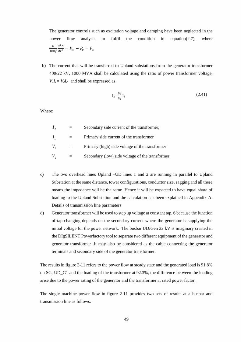
49

The generator controls such as excitation voltage and damping have been neglected in the

power flow analysis to fulfil the condition in equation(2.7), where

𝐻

180𝑓

𝑑2𝛿

𝑑𝑡2 = 𝑃𝑚 − 𝑃𝑒 = 𝑃𝑎

b) The current that will be transferred to Upland substations from the generator transformer

400/22 kV, 1000 MVA shall be calculated using the ratio of power transformer voltage,

V1I1= V2I2 and shall be expressed as

I2=𝑉1

𝑉2I1 (2.41)

Where:

2I = Secondary side current of the transformer;

1I = Primary side current of the transformer

1V = Primary (high) side voltage of the transformer

2V = Secondary (low) side voltage of the transformer

c) The two overhead lines Upland –UD lines 1 and 2 are running in parallel to Upland

Substation at the same distance, tower configurations, conductor size, sagging and all these

means the impedance will be the same. Hence it will be expected to have equal share of

loading to the Upland Substation and the calculation has been explained in Appendix A:

Details of transmission line parameters

d) Generator transformer will be used to step up voltage at constant tap, 6 because the function

of tap changing depends on the secondary current where the generator is supplying the

initial voltage for the power network. The busbar UD/Gen 22 kV is imaginary created in

the DIgSILENT Powerfactory tool to separate two different equipment of the generator and

generator transformer .It may also be considered as the cable connecting the generator

terminals and secondary side of the generator transformer.

The results in figure 2-11 refers to the power flow at steady state and the generated load is 91.8%

on SG, UD_G1 and the loading of the transformer at 92.3%, the difference between the loading

arise due to the power rating of the generator and the transformer at rated power factor.

The single machine power flow in figure 2-11 provides two sets of results at a busbar and

transmission line as follows:

50

i. The output data appearing between UD_G1 and busbar UD/Gen 22 kV from left to right

denotes active power, MW, reactive power MVAR, and current flow, kA. The same is

applicable to power values on the external grid;

ii. The results that appearing between UD 400 kV/UD and Upland ss/400 kV represents the

loading on transmission line and from left to right are voltage, kV, angle in electrical

degrees and current in kA

The receiving end power has been reduced due I2R power loss of the transmission line has been

reduced from 855 MW to 845 MW.

Transient power analysis of power network

From figure 2-11, it has been noted that the equipment associated with power evacuation at fully

capacity of the generator rating at 950 MVA is adequate for loading each transmission overhead

line to external grid. When the power network is operating at steady state the equipment capacity

will sufficient for power delivery to the load. The system is simulated with faults to analyse the

effects of disturbances in the network at three different positions.

Busbar fault at UD 400 kV/UD

A fault was initiated on the 400 kV busbar to last for 0.1 s and open breakers after 5 s.

A disturbance was initiated at busbar as shown in figure 2-12 to isolate all associated breakers

within the 100ms but the power parameters were oscillating beyond the set time of the event. A

Figure 2-11: Results of simulated load flow for single machine

51

very low time was considered in order to analyse the behaviour and characteristics of the

equipment when subject to a disturbance when it is known that protection relays pick fault within

3 or 4 cycles.

The position of the fault has interrupted the generator transformer but virtually looks overloaded

due to the fault current values and all the circuit breakers in the single line diagram have isolated

the fault at the 400 kV busbar. The high loading percent is caused by the high reactive power due

to very high impedance caused by the infinity load on the external grid.

The disturbance on the busbar has affected the generator as it represents about 26% of loading for

the first swing and consequential swings. The system absorbed the reactive power during the

interruption due reactance that was induced by the fault current.

Figure 2-12: Simulation fault results of three phase fault on 400kV busbar

52

Figure 2-13: Indicating oscillation of active and reactive power after disturbance

Figure 2-14: Rotor angle and speed behaviour after disturbance on busbar

53

Figure 2-13 indicates that system parameters are oscillating after the disturbance has occurred but

the rotor angle and speed were too affected refer to figure 2-14. It can be noted that the rotor

angle and speed are also damping oscillating

The change of speed for 1.5% from the figure has affected the parameters and deviated the rotor

angle to increase to about 40% hence causing the machine to oscillate after a disturbance has been

cleared within 100ms.

Faults on Transmission line

The power system can be subjected to a disturbance at any point in the network. However, a

disturbance on the transmission line is considered and analyse the effects of power to the network.

It is common practice on the take-off transmission line surge arresters are installed to divert excess

voltage into the ground .The surge arrester will erupt and conduct to the ground through the

earthing bond of the substation . A fault was initiated on UD_Upland #2 at the position indicated

in figure 2-15 at the same time of 0.1s and delayed the isolation time on the circuit breakers.

Basing on the results in figure 2-15 the disturbance of transmission line has affected the

synchronous generator and caused overloading due to overcurrent on the generator that has

increased its value to 29kA instead of the nominal current of 24kA, the delay to isolate faults may

slowly cause damage to the stator windings. The UD_Upland #1 has been loaded to 54.5% due

to reactive power and visibly there was fault reactance that has been transferred to un-faulted line

hence the overload between the generator and its transformer.

Figure 2-15: Single phase fault on Transmission line near the busbar

54

Figure 2-16 refers , it indicates the overshoot of a rotor angle and speed of the synchronous

machine UD_G1 due to delay initiated to isolate the fault by opening the circuit breakers hence

the overshoot started at almost 24 s on the rotor speed that also caused instability of active power

from figure 2-17. At the same time of 24s, the reactive power started to increase due to fault

reactance.

Figure 2-16: Rotor angle and speed after fault at transmission line

Figure 2-17: Simulation results of single phase fault close to close busbar

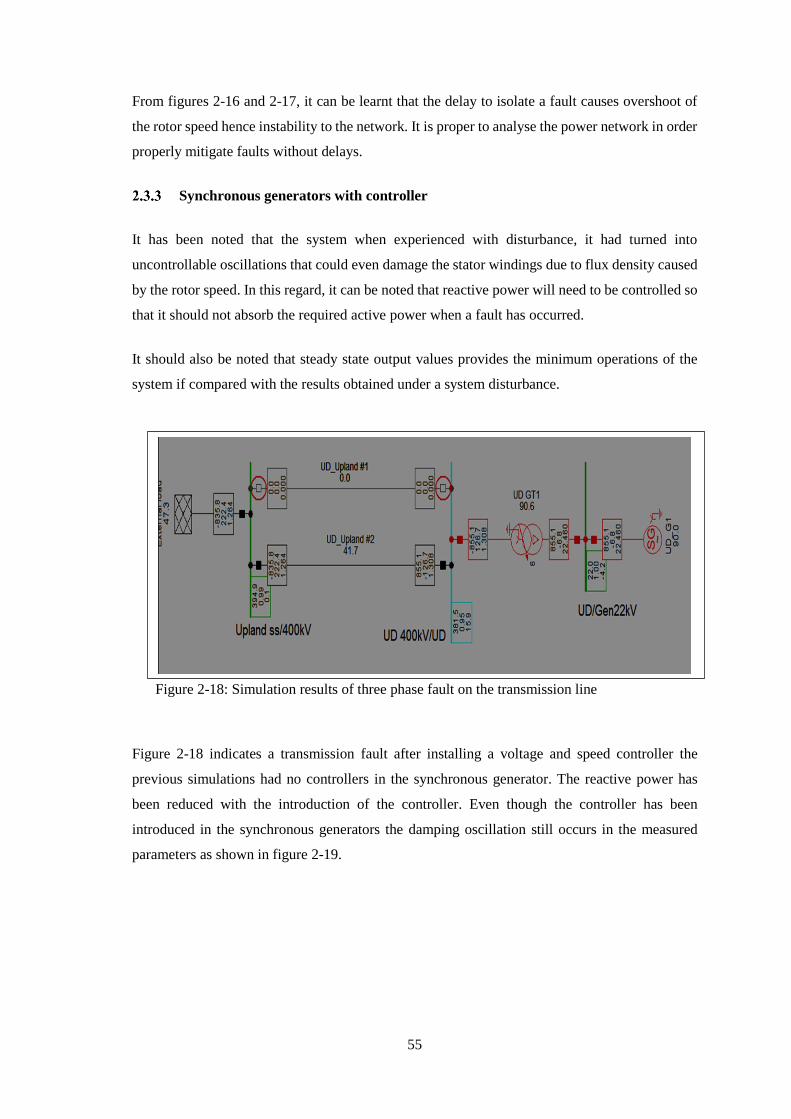
55

From figures 2-16 and 2-17, it can be learnt that the delay to isolate a fault causes overshoot of

the rotor speed hence instability to the network. It is proper to analyse the power network in order

properly mitigate faults without delays.

Synchronous generators with controller

It has been noted that the system when experienced with disturbance, it had turned into

uncontrollable oscillations that could even damage the stator windings due to flux density caused

by the rotor speed. In this regard, it can be noted that reactive power will need to be controlled so

that it should not absorb the required active power when a fault has occurred.

It should also be noted that steady state output values provides the minimum operations of the

system if compared with the results obtained under a system disturbance.

Figure 2-18 indicates a transmission fault after installing a voltage and speed controller the

previous simulations had no controllers in the synchronous generator. The reactive power has

been reduced with the introduction of the controller. Even though the controller has been

introduced in the synchronous generators the damping oscillation still occurs in the measured

parameters as shown in figure 2-19.

Figure 2-18: Simulation results of three phase fault on the transmission line

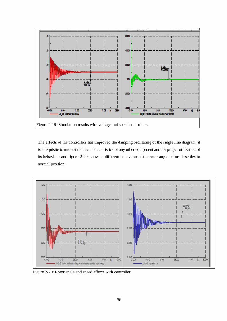
56

The effects of the controllers has improved the damping oscillating of the single line diagram. it

is a requisite to understand the characteristics of any other equipment and for proper utilisation of

its behaviour and figure 2-20, shows a different behaviour of the rotor angle before it settles to

normal position.

Figure 2-19: Simulation results with voltage and speed controllers

Figure 2-20: Rotor angle and speed effects with controller

57

From the results obtained in the simulation, it can be concluded that when the system is disturbed

damping oscillations due occur and cannot be neglected as stated in equation (2.6), where

2

2

dt

dMPPP ema

and this equation considers only the first swing whilst the other decaying

oscillation are not considered.

The transmission guidelines provided by the South African grid code states that the HV breaker

tripping and fault operation of the unit clearing times shall include breaker operating times,

depend on system conditions [55] and shall be as follows:

a. 80ms where the point of connection is 400 kV or above

b. 100ms where the point of connection is 220 kV or 275 kV

c. 120ms where the point of connection is 132 kV and below.

Basing on the guided breaker clearing time plus the protection graded times, then the actual

clearing will be higher than 0.12 ms. The breaker time can apply on the instantaneous tripping

and during the fault time the system will be oscillating waiting for the isolation.

Fault analysis on single line diagram

The results of the simulated single line diagram on faults at different positions indicate a decaying

damping oscillations occurring on the generator rotor speed and angle in return affects the power

parameters such as voltage and current.

When the fault occurred, the parameters immediately changed its amplitude to a first swing and

subsequent damping oscillations of the power parameter. The first (highest ) amplitude is derived

from power dissipation by the resistance of the generator, and then subsequent oscillations are

due to system frequency imposed on the oscillatory torque of the generator rotor due to unilateral

direction components to the machine [56].

When a disturbance occurs on the system, the generator will require to balance up the kinetic

energy that causes the mechanical torque and the potential energy derived from the kinetic energy.

The balance of energy decay causes the magnetic energy in the generator circuit to increase due

to fault that has occurred in the system and the rotor speed will oscillate in the first cycle with

highest amplitude and the rest cycles in the decayed oscillations[10].

58

2.4 Damping oscillations in the overhead line

In electric circuit theory, the nature of the waveforms is called damped sinusoid due to excitation

and forced functions as shown in figure 2-20, the following formula is derived

𝑣 = 𝑉𝑚𝑒𝜎𝑡 cos(𝜔𝑡 + 𝜃) (2.42)

Where

𝑣 = instantaneous voltage

𝑉𝑚 = maximum voltage

σ = neper per second

𝜔 = radians per second

From the principles of RLC circuits of a second order linear system[7, 57] it can be emulated to

the transmission line with RLC parameters at any substation to be represented as a node of the

circuit and voltage drop is calculated as follows:

𝑑2𝑣0

𝑑𝑡2+ (2𝜁𝜔𝑛)

𝑑𝑣𝑜

𝑑𝑡+ 𝜔𝑛

2𝑣𝑜 = 𝜔𝑛2𝑣𝑖

(2.43)

Similarly the equation is presented as follows

Where:

n = LC

1

= the undamped natural frequency

= )/(

2/

CL

R

= damping ratio

𝑣𝑜 = initial voltage

𝜆2 + 2𝜁𝜔𝑛𝜆 + 𝜔𝑛2=0 (2.44)

59

𝑣𝑖 = instantaneous voltage

The undamped natural frequency shall oscillate with constant amplitude because it depends on

the inductance and capacitance of the transmission line .The undamped natural frequency is also

called a resonant frequency.

Furthermore, the undamped natural frequency depends on the line constants and when disturbed

the electromagnetic of the parameters will cause the disturbance to propagate at almost the speed

of light. If the equations (2.19) and (2.29) are substituted in the undamped natural frequency,

𝜔𝑛 =1

√𝐿𝐶 then the speed of light is achieved where it approximately to

81000.3 rad/ sec

Therefore, the disturbance on the system shall travel at the speed of light throughout the network

of synchronised grid due to an equivalent calculation of the undamped frequency.

Naturally, the system response will rely on the damping ratio, 𝜁 and any variation on the ratio

shall also change the frequency of the system, 𝜔𝑛 and the time scale will be adjusted accordingly.

The equation (2.44) is second order differential with real and different roots to a quadratic

equation hence can be solved by formula, and

𝜆 = −2𝜁𝜔𝑛 ± √𝜁2 − 12

(2.45)

When the damping ratio in the above solution of quadratic becomes, 𝜁 < 1 then the eigenvalues

solution will be a conjugate complex and be equal to

𝜆 = −𝜁𝜔𝑛 ± 𝑗𝜔𝑛 √1 − 𝜁22

Where:

= eigenvalue

= damping ratio

n = undamped frequency

It all means that the conjugate complex pair of eigenvalue is given [7]by

60

𝜆 = 𝜎𝑖 ± 𝑗𝜔 (2.46)

Where:

i = integer number and

= f2 oscillatory mode

i = real part of the complex in neper per sec

When the real part of the complex is negative, –σ𝑖 then the system is stable and the damping

frequency, ζ will be represented by the actual or damped frequency at a ratio of

𝜁 =−𝜎

√𝜎2 + 𝜔2 (2.47)

In general terms, it’s imperative to understand the power system stability behaviour during a time

when the sudden change has occurred in the system in order to analyse the pre and post change

of load and generation even more on the interconnected system. It has been noted in the above

sections, after system disturbance the power network, undergoes into damping oscillations and

settles with a new operating condition.

2.5 Calculations of parameters in synchronous generator

Figure 2-10 refers, a synchronous generator, 950 MVA generating at a voltage of 22 kV and

stepped up by the transformer. Considering the generated voltage to be 𝑉1∠𝛿 and the voltage

generated with a load angle of 𝛿, the voltage at the load side be presented as 𝑉2∠0.

Let 𝛿 be load angle that leads 𝑉2 at the infinity busbar, at the furthest end of the circuit to the right

hand side, so that when 𝛿 changes during the disturbance then the rotor will oscillate as the

voltage, 𝑉′ provides a reference phasor , therefore the current flow is calculated as follows:-

It =

V′∠0° − V2∠ − δ

jXT=

V′ − V2(cos δ − jsin δ)

jXT

(2.48)

Equation (2-1) refers, ema TTT where on steady state the mechanical power was equal to

electrical power, further to the equation it can be included that the electrical torque will be equal

to electrical power because of the air gap that exists between the rotor and stator, the notion will

take to the attention of a fact that when the stator resistances is considered negligible and then:

61

𝑇𝑒 = 𝑃 =

𝑉′𝑉2

𝑋𝑇sin 𝛿

(2.49)

When the operating condition changes under a disturbance the load angle will change from its

operating condition to a new condition hence load angle become 𝛿 = 𝛿0

∆𝑇𝑒 =

𝜕𝑇𝑒

𝜕𝛿∆𝛿 =

𝑉′𝑉2

𝑋𝑇cos 𝛿0 (∆𝛿)

(2.50)

The change of operation will be required to be expressed in state space format where the power

system will be analysed on the dynamic performance. Equation (2.7) refers,

em PPdt

d

f

H

2

2

180

will be required to add the component of damping that should be

proportional to the speed of the rotor.

𝑝∆𝜔𝑟 =

1

2𝐻(𝑇𝑚 − 𝑇𝑒 − 𝐾𝐷∆𝜔𝑟)

(2.51)

𝑝𝛿 = 𝜔0∆𝜔𝑟 (2.52)

Where:

∆𝜔𝑟 = the change of speed in per unit

𝛿 = the rotor angle in electrical radians.

The angle is referenced to the synchronous rotating such a-axis in figure2

𝜔0 = the base rotor electrical speed in radians/s

𝑝 = the differential operator 𝑑 𝑑𝑡⁄ with time in seconds

Equation (2.51) has to be linearized and requires to substitute with ∆𝑇𝑒 in equation (2.50) so that

𝑝∆𝜔𝑟 =

1

2𝐻(∆𝑇𝑚 − 𝐾𝑠∆𝛿 − 𝐾𝐷∆𝜔𝑟)

(2.53)

Where:

𝐾𝑠 = the synchronizing torque coefficient

𝑉′𝑉2

𝑋𝑇𝑐𝑜𝑠 𝛿0

62

Equation (2.52) will be linearized with

𝑝∆𝛿 = 𝜔0∆𝜔𝑟 (2.54)

Expressing the equation (2.53) and equation (2.54) into vector matrix:-

𝑑

𝑑𝑡(

∆𝜔𝑟

∆𝛿) = [

𝐾𝐷

2𝐻−

𝐾𝑠

2𝐻𝜔0 0

] (∆𝜔𝑟

∆𝛿) + (

12𝐻0

) ∆𝑇𝑚

(2.55)

Equation (2.55) refers to have the input state space as provided in equation as follows

�� = 𝐴𝑥 + 𝑏𝑢

𝑦 = 𝑐𝑥 + 𝑑𝑢

However, the solution had a second order differential equation that was solved by quadratic

formula, the solution to the equation (2.55) can be solved by the use of Laplace transformation

and will be able to provide the stability control block diagram that can be used for dynamic

analysis for the synchronous machine.

When the load angle changes, the initial operating in reference to E’ and δ and then by using the

simple method where equation (2.53) shall be used to find the solution by Laplace and after also

substituting in the equation (2.54), ∆𝜔𝑟 and results will be in equation (2.56).

∴ ∆𝜔𝑟 =

∆𝛿

𝜔0

∆𝛿 =

𝜔0

𝑠[

1

2𝐻𝑠(−𝐾𝑆∆𝛿 − 𝐾𝐷∆𝜔𝑟 + ∆𝑇𝑚)]

(2.56)

=

𝜔0

𝑠[

1

2𝐻𝑠(−𝐾𝑆∆𝛿 − 𝐾𝐷𝑠

∆𝛿

𝜔0+ ∆𝑇𝑚)]

𝑠2∆𝛿 = −

𝐾𝑆

2𝐻𝜔0∆𝛿 −

𝐾𝐷

2𝐻𝑠 ∆𝛿 +

𝜔0

2𝐻∆𝑇𝑚)

Therefore the characteristic equation is given by the parameters for the synchronous generator

𝑠2 +

𝐾𝐷

2𝐻𝑠 +

𝐾𝑆

2𝐻𝜔0 = 0

(2.57)

Where:

𝐾𝐷 = damping torque coefficient in torque per speed deviation

63

𝐾𝑆 = Synchronising torque coefficient in per unit torque per radians

𝐻 = Inertia constant, H

𝑠 = Laplace operator

𝜔0 = Rated speed in electrical radians= 2𝜋𝑓0 = 2 × 𝜋 × 50

∆𝛿 = rotor angle deviation in electrical radians

A similar notation of damping oscillation format is obtained which has been derived in equation

(2.57) and introduce the K factors that are used for the designed control for the machines.

Therefore, the undamped natural frequency is presented as

ωn = √Ks

ω0

2H

2

(2.58)

Where:

Damping ratio ζ =

1

2

KD

2Hωn

(2.59)

=

1

2

KD

√2HKsω0

When the synchronising torque coefficient varies the natural frequency will vary correspondingly

but the damping ratio vary in opposite direction because it depends on the speed deviation from

the damping torque coefficient. Therefore a high value on the inertia constant will decrease the

damping ratio and natural frequency and of course it inertia constant is the designed value of the

generator.

Modal analysis for power system network

Modal Analysis uses its calculation to obtain the power oscillation of the network by use of the

eigenvalues and eigenvectors[7] that have been computed after the natural oscillation has

occurred on the steady and transient states .

The modelled SAPP grid have over 500 state variable for calculation in the Powerfactory software

tool. The calculation of eigenvalues and eigenvector are based on the complex frequency

discussed in section 2.5 where the solution of the quadratic equation (2.58) is solved by use of

matrix to determine the stability analysis.

64

There are two methods used for computation of the modal analysis used to determine the dynamic

stability of the power system [49]:-

(a) QR/QZ method is used to compute the eigenvalues of real non-symmetrical matrices and

used for the purpose of analysing the small signal stability hereafter referred to dynamic

analysis. It calculates hundreds of state variable of the power system network the

eigenvectors to find the solution small disturbance in the linear characteristics.

(b) Arnoldi/Lanczos method is generally used to carry out selective method calculations of

the system eigenvalues for the power system. It is easy to identify the critical areas.

Simulated modal analysis of single generator

The QR/QZ method was used to calculate the stability of the power system and the results are

shown in figure 2-21. It can be noted that there are over 10 modes to be analysed for its

characteristics and behaviour on single generator. It means that a power system such as SAPP

with almost 10 generators will be populated with modes. This will give a difficult task to analyse

each and every mode plotted.

Figure 2-21: Illustration of stability plot in modal analysis

65

(a) From figure 2-21, the complex representation is provided in the rectangular form and as

such from equation (2.46), the complex pair of eigenvalue λ=-0.2878642+j6.95602

(b) the polar coordinates of the eigenvalue shall be solved mathematically from the polar

coordinates where it is the square of the real and imaginary parts of the above bullet as

𝝈 = √−0.28786422 + 6.956022

ω = arctan6.95602

−0.2878642 .

Polar coordinates have been representing as 6.961973∠180∘ − 87.6302543∘.

(c) damping frequency refers to equation (2.47) and results to

-0.2878642

√√−𝟎.𝟐𝟖𝟕𝟖𝟔𝟒𝟐𝟐+𝟔.𝟗𝟓𝟔𝟎𝟐𝟐2

The period time =2𝜋

𝜔 =

2𝜋

6.95602;

(d) DIgSILENT calculates the ratio amplitude by referencing to the next oscillation and used

the following formula

σ𝑖 =

1

𝑇𝑝. ln ((

𝐴𝑛

𝐴𝑛+1)

(2.60)

Where

𝐴𝑛 and 𝐴𝑛+1are amplitudes of two consecutive swing maxima or minima respectively.

After obtaining the natural modes, the system will exhibit oscillatory stability by the conjugate

complex that has been subjected to complex frequency to provide the damping of the rotor to be

plotted in the complex or s plane The stability of the plotted graph will lie on the negative real

part on the left hand of the complex plane, s shown in figure 2-22 denoting electromechanical

oscillation being stable on the simulated generator[7, 58].

In figure 2-21, the stability of the system lies on the left-hand side due to local oscillation mode,

it lies on the plane of 180°. The generator requires being implemented with stability control so

that it should operate in the second plane of 90 degrees.

66

CHAPTER 3

MODELLING AND OPERATION OF SAPP GRID

Power system modelling is the representation of all system components and elements in a standard

electrical diagram with graphical symbols as provided by the National Regulator of South Africa

incorporation with South Africa Bureau of Standards on NRS 002 [59]and has been used to

represent SAPP network. The graphical single line diagram is used for the power flow studies

which provides information on the voltage magnitude and angle at each bus and real and reactive

power at different nodes.

SAPP grid has been interconnected to different national power systems and covers geographic

surface area of over 1,219,912 square kilometres[60]. When modelling to study different

performance measurement, it is not a prerequisite to detail the entire network[61]. This is due to

the available speed of the operating system of the computers that might slow down due to iterative

methods to calculate the solution for the required assessment. The dynamic analysis will require

to analyse performance of the synchronous generators. Therefore, the interconnected generators,

transmission lines and load were modelled for the SAPP dynamic analysis.

DIgSILENT, a short-form abbreviation of DIgital SImuLation of Electrical NeTworks is one of

the computers aided electrical engineering tool used in power system modelling and analysis. The

Powerfactory tool is a licensed software from DIgSILENT. It is used for parameter calculations

and analysis of transmission, distribution, and industrial electrical power systems with an

integrated graphical single-line interface. The software is designed with integrated and interactive

software package for practical usage of the electrical power system and control

The interactive single-line diagram means that it is possible to model by utilizing the drawing

functions embedded in the software tool, editing capabilities of the required data for any

equipment including calculating from the diagram and entered data the solutions for all relevant

static and dynamic calculation features studies.

The DIgSILENT Powerfactory software tool has been used for the study of the SAPP grid because

it’s the most common software tool used in the Southern Africa, by organizations involved in

planning, consultants, and educational institutions in South Africa.

67

3.1 Parameter for modelling in dynamic studies

When modelling the SAPP grid, it is necessary to have a knowledge of the generators, substations,

transmission lines and load. It is also necessary to know the data for various equipment for the

designed model. For a massive network as the SAPP, it is not feasible to acquire all the data for

the high voltage and secondary control equipment. Thus, a reduced order model of the SAPP

network was analysed and using the dynamic model of the generators. The available data

acquired have been detailed in the appendices A and B for the generator and transmission

lines.

Direct energy transfer functions on generator

In carrying out stability analysis, the mechanical energy in the power network also plays

a vital part on the oscillation of the turbine and rotor shaft in the synchronous generators.

In case of severe disturbance, machine energy functions have been studied to acquire the system

transient energy for direct method by use of Lyapunov functions [62]. The direct energy transfer

method tend to provide the transfer of mechanical energy to oscillate and be absorbed by electric

energy without losing synchronism. The direct energy function is developed based on the

conserving energy on the use of mechanical energy should operate within the limits and any

oscillation should settle on within the limits set on an individual generator [63] This can be likened

to the releasing of a body of mass from a top on a saddle to accelerate and come to rest. Similarly

the energy functions were using the synchronous generator frame as reference in the mathematical

derivations from equation (3.61) the other approach was to identify the centre of inertia where all

the critical fault should be directed to the machine. Therefore analysing this direct method of

energy functions it is required to:-

a) Determine accurately the unstable equilibrium area; and

b) Determine a sound proof that the mechanical energy functions can cause system outage.

Similarly to equation (2.11) refers, the motion of generator is represent as

ie PPdt

dK

dt

dM

2

2

This can be expressed in terms of speed so that

𝑀𝑖

𝑑2𝜔𝑖

𝑑𝑡2+ 𝐾𝑖

𝑑𝛿

𝑑𝑡+ 𝑃𝑒𝑖 = 𝑃1

(3.61)

68

Where:

= angle of voltage behind transient reactance indicative of generator position

i = rotor speed

iM = generator Inertia Constant

iK = damping coefficient

i = 1, 2, 3…..n

The approach to transfer energy functions to electrical circuits from speed is very difficult to be

achieved because requires to identify the centre of inertia of the multi-machine. The

interconnection power network is dynamic and as such critical group of machines that have been

referenced as the centre of inertia can change due to complex variations of the system[62].

However, the use of Lyapunov function to analyse as a direct method is still understudy and the

method will not be used for the dynamic analysis. The transient analysis involves severe faults

that require protection system to isolate and dynamic analysis involves the changes that take place

by the controller to adopt the sudden changes of load and also during the fault to remain in

synchronism. Therefore the direct method is still being studied on transient analysis, the

modelling studies have not justified whether a system remains in synchronism after disturbance.

The method shows mathematically efficient alternative to time domain simulations. Even though,

the developments show that direct method by Lyapunov functions can offer alternative computing

on real-time time-domain simulations, the methods has lurked development to provide analytical

insight into the behaviour of power systems and providing theoretically principled estimates for

power system stability[64].

Rotor equivalent electrical circuit

Powerfactory software tool uses the stator and field winding electrical circuits for modelling the

dynamic stability analysis. The equivalent circuit diagrams of the standard synchronous machine

is referred to the rotor system and presented in the Park coordinates dq – reference frame. There

are two axis modelled, the d-axis for the two rotor loops on the rotor representing the field

excitation winding and one damper winding on the q-axis on salient rotor. The round rotor will

have two damper windings[65]

69

Where:

strr Stator resistance

fdr Resistance field windings

dr1 Resistance damper winding d axis

qr1 Resistance damper winding q axis

lx Stator leakage reactance

adx Reactance of synchronous machine d axis

aqx Reactance of synchronous machine q axis

rldx Mutual reactance between field and damper windings- d axis

rlqx Mutual reactance between field and damper windings-q axis

Figure 3-1: Rotor circuit as represented in DIgSILENT for d-axis

Figure 3-2: Rotor circuit as represented in DIgSILENT for q-axis

70

fdx Mutual reactance between field and d axis

dx1 Reactance of damper windings d axis

qx1 Reactance of damper windings q axis

From figures 3-1 to 3-2, it can be noted that the resistancesfd

r , dr1 , aqr and strr are connected in

series with inductance fdx , dx1 and lx for the field, damping and stator windings. It is based on

the characteristic of the resistance and inductance connected in series that will be fundamental to

the stability analysis. This is contrary to the assumption that was made in the mathematical

deviation that assumed that the voltage behind the stator reactance, lX was fixed at voltage

magnitude. It is the behaviour of current in series of resistance and inductance (RL) circuit

behaviour that will be adopted in the modelling of synchronous generator. The voltage behind

reactance will then be essential applicable on the machines that are interconnected in the power

pool [61, 66].For the interconnected power system to remain coherent, the stator resistance, lX ,

that represents the voltage behind the reactance will be used to describe the dynamic equivalency

technique . The technique will identify the groups of machines and each group will be represented

as the single generator model that will be used to evaluate the coherency analysis of generators

when subjected to a disturbances.

The currents fdi , di1 and di are flowing through the resistance and inductive circuits of the field

winding, damper winding and stator winding. Current flow through the resistance will reduce the

current flow and dissipate heat. The current flow in the inductor will grow its current before

reaching its maximum current. The energy conversion is associated with the change of current

with time such as that dt

diL will be form the magnetic field due to flux generated and flow of

current in the inductor also be used to excite the start of the generator.

The voltage fdV is the voltage that will be used for the change of voltage in the excitation circuit

transformed from the grid and dU will be the generated voltage from the change of flux. d ,

through the stator inductance lX .

71

Figure 3-3 shows the growth of current in the RL circuit that will correspond to the d- axis circuit

provided in figure 3-1. The rate of growth of current at any instant is in such manner that it

continues at an increasing rate and reaches its maximum value of I amperes in R

L seconds.

Hence this period is termed as the time constant of the circuit and is usually represented by the

symbol T [67]. However, time constant are derived when the circuit is closed or open positions.

The generator will use the field winding operation to open and close the regulating voltage circuits

and hence manufacturer will determine and provide the time constant relative to the self and

mutual reactance to the customer.

Due to saturation effects, where current flow will flow from the source of voltage such as the

field winding and stator windings, the resistances provides maximum value whilst the inductor

will be charging to reach its maximum and also provide the discharge path on open circuit.

It can be observed that the generator model will require to determine the equivalent circuit in

order to assess detailed parameters on the effects and merits of the damping, field windings and

excitation control. The dq rotor referenced frame in the generator model for the time domain

simulations will use the rotor fluxes, the synchronous speed and load angle as the state variables.

Figure 3-3: Growth of current in inductive circuits

72

Determination of parameters for model

The equipment that are installed in the network undergo various stages before being

commissioned. The equipment will be designed and specified depending on the studies carried

out for the installation. The equipment will also be tested to verify compliance of the delivered

and or installed equipment. It is normal to keep records relating to design, specifications and

compliance by pre and commissioning tests before energized .The filing and keep safe of such

information will reasonably be required for assessing power system performance (including

actual unit performance during abnormal conditions). Often times the equipment will be tested as

provided by the grid code requirement where a regulatory body established as the technical

requirement.

The conduct of tests and different studies will therefore demonstrate that each high voltage

equipment is regularly checked as a compliance to the technical requirement. In order to have a

common technical approach to the functioning of the network, a regional harmonization code has

to be developed amongst the regulators in the Southern Africa. Such grid code will provide testing

procedures to be carried out on new units, after every outage where the integrity of any grid code

requirement may have been compromised. This will demonstrate the compliance of the unit with

the relevant grid code requirements. The utility shall continuously monitor its compliance in all

required equipment in order to respect the connection conditions of the Grid Code.

Manufacturers parameters

Manufacturers of the power system equipment have different design procedures to run software

packages for the production of the equipment. However the routine calculation of the standard

equivalent circuit parameters are required to be adhered to. The utility and the manufacturers will

reserve the rights to disclose the specifications used for the network. It is then necessary for the

manufacturers to provide a standard reactance and time constants in the direct and quadrature axis

in case of synchronous generators for the utility to use system analysis. If a non-standard method

has been used by the manufacturers, then the manufacturer will require to derive its parameters

for the interest of the utility.

The manufacturers may provide different parameters definitions, symbols and methods of

applications depending to the origin of region of the world. There are instances when for example

sub transient, transient and synchronous reactance are in the format like '"" ,, didvdi XXX and duX

for the direct axis[65] and in the Powerfactory tool have used without subscripts i, v and u. It is

appropriate to understand the notations that have been provided by the manufacturers hence the

quantities means the same as “ i ” the short circuit current equal to rated armature current and

73

designated often as unsaturated parameters. The “ v ” applying to variations associated with faults

due to sudden three phase short circuit from the rated terminal voltage.

The use of the numerical methods are applied for commercial and in house software packages for

the application on its own simulation design to the required specifications. The designed circuits

will be used to predict the required specification and further to the equivalent model. In power

system transient analysis, the utility will normally provide the fault levels at the point of

connection and that will be used for the simulation of the manufacturers but for the dynamic

performance, then the simulated circuit will be used for different operating conditions.

Test result parameters

The testing of equipment in the power system network is challenging because of the high voltages

required to be handled during the tests. However, in case of voltage, it is the low voltage that will

be used and be translated as the ratio of the primary voltage. The secondary voltage from the

testing equipment will be used to be injected on the high voltage equipment for example on 330

kV the maximum secondary voltage 110 volts will be used for injecting supply. The injected

voltage will be proportional to maximum secondary voltage. The dividend is multiplied by the

primary voltage to provide an equivalent of the primary voltage for 330 kV.

The voltage injection can be used to measure reactance in the generator windings if access is made

easily accessible, but a fuse wire should be used to short the other terminals. The fuse wire will

protect the instrument and damage to the windings.

The purpose of testing on equipment does not only imply to obtain the equipment values but also

to checks wiring and operation of the equipment.

Parameters of the synchronous machine used in Powerfactory tool

The parameters used by the Powerfactory tool and are elements shown in the equivalent circuits

in figures 3-1 and 3-2 and detailed in the Appendix B-3. It can be observed that current flow in

the machine circuits are flowing in loop such that there is mutual effects during the operation.

The output current will have the effects of damping and field windings.

From equation (2.16) the per unit stator voltage that provides the generated voltage to the grid

have been expressed as follow:-

74

Further to equation (2.16), rotor voltage equations can be derived from the field winding in figure

2-3, where fdV is determined as source of voltage to the rotor and it has used the normal circuit

calculations[7].

𝑉𝑓𝑑 = 𝑝𝜓𝑓𝑑 + 𝑅𝑓𝑑𝑖𝑓𝑑

0 = 𝑝𝜓1𝑑 + 𝑅1𝑑𝑖1𝑑

0 = 𝑝𝜓1𝑞 + 𝑅1𝑞𝑖1𝑞 (3.62)

Where:

fdV Voltage across the field windings

fdR Field windings resistance

dR1 Resistance damper winding d axis

qR1 Resistance damper winding q axis

lx Stator leakage reactance

fd Flux in the field winding

d1 Flux in the d axis winding

q1 Flux in the q axis winding

p The differential operatordt

d

p Differential difference of flux related to time

𝑒𝑑= p𝜓𝑑– 𝜓𝑞𝑝𝜃 − 𝑅𝑠𝑡𝑟𝑖𝑑

𝑒𝑞= p𝜓𝑞 − 𝜓𝑑𝑝𝜃 − 𝑅𝑠𝑡𝑟𝑖𝑞

𝑒0 = p𝜓0 – 𝑅𝑠𝑡𝑟𝑖0

75

The equations (2.16) and (3.62) have defined the stator and rotor voltage circuits , but it is

required to understand the effect of stator and rotor mutual flux linkages. Powerfactory tool

introduced a variable reactance adX and aqX in the d and q axis equivalent circuits figures 3-1

and 3-2. In other explanations of parameters on mutual reactance adX and aqX are provide at a

fixed value. The variable reactance will be used for parameter conversion of short circuit to

equivalent circuit parameters and for the mutual linkages then

𝑥𝑎𝑑 = 𝑥𝑑 − 𝑥𝑙

𝑥𝑎𝑞 = 𝑥𝑞 − 𝑥𝑙 (3.63)

Where:

adX = mutual leakage reactance on d axis

aqX = mutual leakage reactance on q axis

lx = stator reactance

dx = reactance on d axis

qx = reactance on q axis

The arbitary variables are introduced in the powerfactory tool for the mutual reactance in order

to introduce to new variable after disturbances. The new variable will be used for the dynamic

analyis and other applicable studies.

76

Table 3-1: Typical values of generator parameters

Symbol

definitions

Description Expected Values on

Synchronous[7, 8]

PF STD Thermal

Hydro

strr strr Stator resistance 0.0015-0.005 0.002-0.02

lx lx Stator leakage reactance 0.1-0.2 0.1-0.2

rlx rldx Mutual reactance between field and damper

windings- d axis

rlqx rlqx Mutual reactance between field and damper

windings-q axis

dx dx Synchronous reactance d -axis 1.0-2.3 0.6-1.5

qx qx Synchronous reactance q axis 1.0-2.3 0.4-1.0

dsx '

dx Transient reactance d- axis 0.15-0.4 0.2-0.5

qsx '

qx Transient reactance q- axis 0.3-1.0 -

dssx "

dx Subtransient reactance d- axis 0.12-0.25 0.15-0.35

qssx "

qx Subtransient reactance q- axis 0.12-0.25 0.2-0.45

dst '

dt Short circuit transient time constant d-axis 3.0-10.0s 1.5-9.0s

qst '

qt Short circuit transient time constant q-axis 0.5-2.0s -

dsst "

dt Short circuit subtransient time constant d-axis 0.002-0.05s 0.01-0.05s

qsst "

qt Short circuit subtransient time constant q-axis 0.02-0.05s 0.01-0.09s

From table 3-1, when the short circuit transient time constant is not provided by the

manufacturers, then the short circuit subtransient can be entered. The short circuit time constants

are the most important parameters because will provide saturation at the loading of the generator.

The subtransient is normally called the open loop time constants and will require to be converted

as short circuit parameters as follows:

𝑡𝑑

" = 𝑡𝑑0"

𝑥𝑑"

𝑥𝑑′

77

𝑡𝑞

" = 𝑡𝑞0"

𝑡𝑞"

𝑥𝑞′

𝑡𝑑

′ = 𝑡𝑑0′

𝑥𝑑′

𝑥𝑑

𝑡𝑞

′ = 𝑡𝑞"

𝑥𝑞,

𝑥𝑑

(3.64)

For the salient synchronous machine, the transient reactance '

qx and the transient time constant

'

qt in q–axis are not required due to unequal values and saliency effectiveness not significant

on the generated voltage, stator current, power and excitation over normal operating point.

Therefore subtransient time constant "

qt is then calculated using transient reactance qx on q axis

instead of the subtransient reactance on q axis.

The behaviour of the synchronous machine when subjected to the three phase fault will respond

in the electrical transient characteristics. The existence of resistance and reactance in the

synchronous machine ensure that current will not grow spontaneously but with slow growth due

to flux in the reactance windings. When the synchronous machine is disturbed then the flux will

still be slowly discharging through the resistance. However, the slowly decaying of ac component

is due to the relatively slow decay of the flux linking the transient circuits.

Synchronous machine models have been used in Powerfactory tool with a number of different

investigations undertaken to analyse adequately the parameters with various techniques by both

models on mathematical and experimental on the actual machines. Several assumptions have been

made in the evaluating the synchronous electrical parameters and as such theories have been

derived when determining the parameters [68, 69]. The development of mathematical model has

resulted in the development of the Powerfactory to be able to simulate the machine tests on

different types of analysis required for system design, planning and operation.

It can easily be noted that the common assumptions made during the test corresponds to the study

of dynamic analysis. The machines were tested on sudden 3 phase short circuit on the generator

terminal and stator decrement test with field winding short circuit amongst the assumptions made

during the investigations.

The understanding of measurable time constants will not suffice the determination of direct axis

circuit parameters but will need to carry standard tests to make approximations[69] .It is for this

reason arbitary variables are introduced in the powerfactory tool for the mutual reactance such as

1x , 2x , 3x , 1T , 2T , a and b have been introduced for the determinaton of direct axis[49] . The

78

mathematical calculations derive the damping time constants that is related to equation (2.57),

where a second order equation was achieved through the single line diagram

𝑠2 +𝐾𝐷

2𝐻𝑠 +

𝐾𝑆

2𝐻𝜔0 = 0

It is through the mathematical derivations that has produced the second order polynomial

equation. There are various ways of determining its values

𝑇𝜎𝑓𝑑 =−𝑎

2+ √

𝑎

4

2

− 𝑏

(3.65)

Where:

ldT = Mutual Time constant between stator and damper windings

fdT = Mutual time constant between field and damper windings

ba, = approximated variables.

The equations described for a single machine system but the SAPP power stations are often

comprised of six machines utmost per station. When modelling the generators, the number of

machines at a station will be presented to provide the general picture of once off simulation on

the system operations.

3.2 Power system monitoring instruments

The accurate measurement of the voltage, current, frequency, power, phase angle depends on the

requirement for the power system. The measurements provides power system control ranging

from automatic closed loop control to recording of data for statistical purposes. The measured

parameters provides direct visual reading as well as processed reading for remote from electrical

measuring transducers.

𝑇𝜎𝑙𝑑 =−𝑎

2− √

𝑎

4

2

− 𝑏

79

Transducers are used as interfaces to generate an accurate small direct current analogue output

usually in milliamps which corresponds to the parameter being measured. Unlike, tapping directly

from the secondary output of the current and voltage transformers require isolation points in form

of shorting and links respectively. The transducers provides a galvanic isolation quote the book

of sourcing between the input and output. This provides and advantage to the output requirements

to have light specified insulation requirements.

The outputs of the transducer are used for a simple presentation of measured values for the system

operator in the Control Area and SAPP Control Centres to determine system control strategy.

However the same values are used for the automation scheme in power control system such as

Automatic Generation Control (AGC), Automatic Voltage Regulator (AVR), plotting of

disturbance recorder.

Input source of a transducers

The transducer obtains its input from current and voltage transformers installed either outdoor or

indoor substations. For overall accurate measurements of the transducer, the input originates from

the metering class instrument transformers. There are normal two types of current transformers

metering and protection instrument transformers that differs on accuracy. It is also common to

apply transducers on protection class instrument transformers and this has characterized to

withstand significant short term overload on their current inputs. It can also withstand up to 300

% of full load continuously hence the input circuit will be staggered at low impedance for current

and high impedance for voltage input.

Output signal of a transducer

The output signal of the transducer is usually current and common ranges are 0-10 mA, 0-20 mA

and 4-20 mA. This means that the required parameters have to be programmed to suit the ranges

of values to be monitored. It means also that in case of voltage range of the transducer can be

added to display devices without limits and without any need of adjustments of the transducer.

The value of voltage range determines the maximum loop impedance of the output circuit. Hence,

when the voltage range is high then it facilitates remote location of an indicating instrument.

In case of the output of the transducer being used for control purposes then measurements are

placed to avoid open circuit in the internal circuitry. When the transducer is faulty, a constant

current is continually injected to raise the voltage and provide falsified values in the loop for

monitoring the power system.

80

Accuracy of transducers

Transducer plays an important role in providing the system operator with measured and monitored

parameters. The Supervisory, Control, and Data Acquisitions (SCADA) depend on the output of

the transducer to acquire data for the control of the power system. The accuracy of the transducer

varies in the essence of the condition to be used on the power system and depends on how it’s

closely monitored and operated at all times.

The accuracy of the transducer is affected by factors that can be ignored or not to be relevant but

the user have little or no control of it. This factors include the ambient temperature, external heat,

input quantity distortion and unbalanced input[70]. The accuracy of a transducer is checked under

an agreed set of conditions known as reference conditions. The intrinsic error is determined under

reference conditions. All the transducer with the same intrinsic error are expressed as percentage

such that a transducer with an intrinsic accuracy of 0.1 % of full scale has a class index of 0.1[71].

The transducer provides improved communication facilities where it allows several types of

transducer to be transferred in the same link. The programmable scaling is done remotely without

interference of the plant in the substations.

Under disturbance in the system the transducer will not provide the output signal immediately

and it will take to time to respond to the change of the power system. This is due to the

transformation that is undertaken in the transducer to provide an indication. The transducer will

take a value from its source for example if the current is 0.8A from a full secondary current of 1A

it has to reproduce an output of 8mA dc. Then when immediately a disturbance has occurred it

takes time to readjust what is being processed.

Current transducer

The current transducer is connected to the secondary of instrument current transformer with an

input of 1 and 5 amps. The current transducer provides the loading of the power system in

amperes. The current transducer provides indications to the indicating instruments proportional

to the input.

(a) Primary current = 300A

(b) Secondary current = 1A

(c) Transducer input = range of 0 – 1A secondary of (a)

(d) Transducer output = range of 0 – 10mA

(e) Current input of transducer = 0.84A measured in (b) and (c)

(f) Transducer actual output = (b) x(c)

81

= 0.84 x 10

= 8.4mA

(g) Actual current flow = (a) x (d)

= 0.84 x 300

b) Current flowing in the high voltage = 254 A

The current flow in the power network is unidirectional. It is very difficult to know the direction

of current flow whether it’s being imported or exported in an interconnected power pool.

Voltage transducer

The voltage transducer is connected to the secondary of an instrument voltage transformer with

an input of normally 110 volts and 63.5 volts on high voltage transmission line. The voltage

measurement in the power system is usually at the rated high voltage with ± 10%. For this reason.

The voltage transducer has a suppressed zero type of measurement. It provides the voltage at

specific range. In case of synchronizing voltmeter, the indications are provided in the inverse

linear to assist in synchronizing the generators into the grid.

Measurements of voltage using the transducer becomes different and requires careful

considerations.

(a) Primary voltage = 330 kV

(b) Voltage transformer = 330 kV/110 V phase to phase

(c) Voltage transducer - Input = 0 -10 mA

= 110 V/10 mA

If (c) is considered for the output of transducer, then at 330 kV will be the maximum voltage

indications. The voltage fluctuates on the network and as such measurements for the transducer

require to further extend the output range. Then, this provides the readings on the indicating

instruments compatible to changes of voltage in the system.

However, the voltage range input for the transducer need to be extended reasonably. When it is

considered as the required statutory requirements of ±5%. The design of the transducer will be

different from the standard output for the transducer. The accuracy of the transducer will depend

on the requirements of voltage measurement. Mostly the voltage output is ranged up to 150 V.

(d) Voltage transducer input = 150 V/10 mA

82

(e) Primary voltage can be measured = 450 kV

The statutory requirement for the measurement of the power system is beyond the standard that

had been determined in the SAPP Contingency Analysis[36]. It’s very difficult to carry primary

injection at very high voltage. The only secondary test will be carried to confirm the right

measurement of voltage is indicated on the instruments. It is required to recalibrate the voltage

transducers with the real time frequency response to ascertain the accuracy with the subscribed

input of the transducer[72].

The output for the voltage transducer becomes more complex when the 4-20 mA is used as the

output of the transducer. This is due to upper reading of 4 mA output from the transducer at zero

reading. This type of transducer has a fixed reading that does not consider the over range

adjustment as mentioned in (d) of the voltage transducer. This type of transducer adjusts the

primary voltage to suit the maximum of the transducer output.

If the indications are not scaled properly, it will then provide unrelated monitoring information

for the power system. The general rule for measurement, the full primary value should be directly

proportional to the full indication of the instrument. If the full input to the transducer has drifted

away then the indicated value will not remain the same.

Synchronization

This voltage measurement is very essential in the power system. It is the same voltage that is

required for synchronizing torque coefficient required for the electrical power to absorb the load

as defined in equation (3.66)

sin2

'

T

eX

VVT

(3.66)

Synchronization is performed at a busbar of different supply sources and angle required to be

connected from a common point of breaking point. In the Interconnected power pool such points

are referred tie bus or tier. The two known place requiring synchronizations are:

1) Generator and grid

2) Two grid supplies connecting on transmission lines

The synchronizer is installed to determine that the two voltages are in synchronism. The two grid

supplies will be monitored by the voltmeter and phasor angle instruments. When the two voltages

are approximately equal to each other and also the phasor angle is zero. The synchronizer provides

83

a close contact to for the circuit breaker separating the two grid. In true sense the voltmeter will

be measuring the magnitude of the voltage and the phasor angle determine equal frequency

between the grids.

Frequency transducers

It has been noted that the voltage and current transducers derives their input for instruments

indications from instrument current and voltage transformers. The combination of the voltage and

current does not provide frequency. However frequency monitoring obtains its frequency from

the secondary output of the instrument voltage transformer. The transducer does sample the rate

of cosine waveforms that crosses zero to provide the frequency of the system. It also determines

the sampling number and value that has crossed zero at specified time to inversely proportionate

for frequency.

Accurate measurement of frequency is quite important to the interconnected power system.

However, most manufacturer provides an error percent of 0.1% and 0.01% for the frequency

indication with a centre zero. The centre zero provides an indication from zero to 50 Hz on right

hand side and 50 Hz to zero on the left hand side.

Phase angle transducer

This type of transducer provides a measurement of power system for the power factor. It is upon

the indication of the power factor when the power angle can be calculated for system. It is

achieved by the input from both the current and voltage instrument transformers. The scaling of

the transducer for the indicating instruments will be centre zero as 180..0..180 the output of

the transducer will then be taken the same format for indicating instruments mAmA 10..0..10 .

This notation of range denotes whether the power factor will be leading or lagging. The output of

mA10 on the indicating instruments means lagging measurement and mA10 means that the

measurement has a leading power factor indication. When the load angle changes then the

indication will be according to the input from the transducer.

In SCADA monitoring, the power factor will be programmed to provide for real value of the angle

and it all depends on the point of measurement, similarly the transducer will use the zero crossing

waveform and provide the mean sample as the power factor value.

84

Power transducers

The power transducers such as the active and reactive power measurement require to realise the

nature of load on the network. The connection of power transducers are shown in Appendix C for

the following type of loads.

i. Balanced load

The balanced load has the behaviour of the delta connection. The current flow in the delta

connection is equal in all phases at I3 and voltage will be the same at phase to phase or

when a neutral is introduced to the system. A separate connection of earth wire provides a

neutral to the 3 phase delta connection. The system is defined as 3phase 3wire balanced

system when phase to phase voltage is used for measurement and 3 phase 4wire balanced

system when the phase to ground voltage is utilized for the input of the transducer

For the delta connection, a single current transformer is installed to measure the power flow

and also a single phase to phase voltage transformer is installed for measurement.

ii. Unbalanced load

The unbalanced load is the star connected load where it is assumed that the phases carry

different current value and there are three different configurations

a) 3phase 3wire unbalanced load

The current transformers are connected to two phases and the voltage transformer

connected to three phase A, B, C thus phase to phase voltage. The current transformer

connection to the phases is being termed 3 phase because 3 wire are connected to phase

A, Phase B and Phase C

b) 3 phase 4 wire unbalanced load

The current transformers are connected all three phases and voltage transformer has been

connected on the three phases including neutral.

c) 3 phase 4 wire unbalanced ( 2

12 ) load

The connection of the current transformer is the same as 3 phase 4 wire unbalanced load

and differs on the voltage connection where only two phases and a neutral are used for

measurement.

The power transducer uses secondary output of current and voltage instrument transformers. The

power transducer also use the multiplier that combines the current, voltage and phase angle to

85

provide the power calculation in the transducer. The output is scaled accordingly to provide the

primary values of the power system.

iii. Scaling of power measuring instrument

The power measurement like the active and reactive is indicated from the product of voltage,

current and phase angle. The scaling will be carried as follows whether balanced or

unbalanced loads.

(a) Current Transformer Ratio = 300A/1A

(b) Voltage transformer Ratio = 330kV/110V

(c) Power factor = 0.8660

= 120° symmetrical components

(d) Primary Power calculation = 3 x current primary x voltage

primary

= 3 x300Ax330kVx0.8660

= 148.5 MW

(e) Secondary power calculation = 3 x1Ax110Vx0.866

= 165 W

(f) Active Power scaling = 150 MW

(g) Reactive power scaling = Power triangle formula

= 22

5.1483303003 MWkVxx

= 225.1484.171 MWMVA

= 85 MVAR

In normal cases, experience has shown that the reactive power is scaled half of the active power.

It becomes contrary to the power triangle calculation. If the transducer is specified as secondary

input of the instruments transformers as in (e) then the transducer will not indicate the 148.5 MW

on the system. The active and reactive power need to be specified as per installed specifications

of the instrument transformers to be applicable and accurate for monitoring on the import and

export of the energy consumption.

86

Energy Metering

Unlike all the above stated instruments, energy meter register and store its consumption and

demand. The others provide only instantaneous measurements

Meters and instrument transformers for energy metering is applicable on metering specifications

as outlined by a Technical committee in International Electromechanical Commission. It is so

specialized form of measurement on electrical power, reactive and for the purpose of trading

within the operating members of SAPP and also consumers

The energy metering read and record active and reactive energy. It presents the energy delivered

to or received at each connection point, with an appropriate degree of accuracy specified in

applicable IEC 60687 to be not less than +/- 0.2%.

The energy metering records power over a number period, so the energy is measured in units of

kWh. The energy meter uses power waveform to register the energy. It picks the peaks and zero

crossing average at an hourly period. The zero crossing are indicated by pulses flashing on the

meter. The energy meter, therefore, specifies the number of pulse rate in one hour. If the pulses

are flashing at fast rate then it means the high usage. The energy meters are programmed to

continue and average the power even if the consumption did not complete the hourly period. This

will enable to register energy consumption.

The maximum load demand is another measurement that is carried out as a power capacity in

energy meter. The meter keeps access memory of all highest peaks in the waveform and sort

accordingly. The maximum load will indicate the highest the meter registered during the billing

period.

The energy metering equipment shall have the following characteristics[73]:

(a) Three phase four-wire system as explained in the power transducer;

(b) Record in the required billing period for power, energy and maximum demand available in

data registry. The recorded parameters should be displayed for reading with its

instantaneous and accumulated data. The meter should be a programmable and reset after

the billing period for the cycle of billing period;

(c) The meter should be able to measure all the four quadrants on reactive power , import and

export on active power to show the direction of power flow;

(d) When a backup register is used, the data register should store separately the information

from different metering points. It should be properly labelled whether main or backup

meter;

87

(e) The data memory in the meter should be able to store at least one year with intervals

programmable from 5 minutes to 30 minutes in non-volatile memories;

(f) The meters should be capable to be interrogated by local ports or telemetering or the

available serial communication for data collection from the meter;

(g) The meter should have the capabilities to provide alarm when tampered , indicate status

when faulty,

(h) Meter shall be at a secure and well protected, visible and accessible, conforms to tropical

environmental conditions. The meter kiosk should be sealed to prevent unauthorised

access.

The metering system provides measurement for the consumed energy and capacity energy on

each installed point. The energy meter provides both import and export metering at all

interconnections of power system. It will provide the main and check meter in case of the failure

of the main meter, the check meter should be referred to take the readings for the billing period..

The main and backup meters should be installed as close as practicable at the installed point and

where the location is placed at different position, SAPP connection agreement should determine

and agree on the adjustment of loss that may incur between the two meters. The adjustments of

the loss should include transformer and line loss compensation.

Disturbance recorders

Power system suffers from different types of disturbance and often times just like indicating

instruments, protection operates without any record for the system operators. The detailed record

of disturbance will enable the post fault analysis determine the nature of the fault. The analysis

will also provide subsequent operations on pre and post faults on the affected plant. A detailed

recording of the fault distinguishes between cause and effect in its plotting. If the effects are

spread over wide area of SAPP grid, records of the disturbance from a number of locations from

utilities can assist to determine the location of the disturbance.

Characteristics of the disturbance recorder

(a) It is characterised with multi-channel analogue input waveform for recording required data.

The analogue channels are provided to record current and voltages on the faults to be

recorded at a substation or generation plant. The waveform that it produces has to be

captured with analogue conversion to digital. This type of recorder have surpassed its

existence in technology.

88

(b) The digital multi-channels are embedded in main protection relays such as distance relay

on the transmission line. They have an advantage to store several records that can be

downloaded for analysis. The digital inputs are provided to capture signals such as circuit

breaker opening, protection relay operation, inter trip, magnitude of current and voltage

during the disturbance;

(c) The triggering effects are made available for both analogue and digital input channel to

record and quantify the occurrence of the disturbance in the power system. It is operational

norms of the disturbance recorder to have relevant threshold to initiate the trigger facility;

(d) The recording time can be programmed to register for disturbance that can last several

minutes. The recorder captures events over a wide range of timescales by programmable

sampling rates. It ranges from the short term transients while also ensuring sufficient data

to be collected on the long term transients; and

(e) Time synchronization is also vital on interconnected network so that faults time are aligned

from one recorder to the other of the same event.

3.3 Technical operations of SAPP Grid

The objective of SAPP guidelines ensure that operating members participate and benefit from

the pool in an environmental that will be in sustainable manner .It also equally operate the electric

power network of Interconnected power pool such as Southern African Power Pool (SAPP)

safely, efficiently and effectively.

Therefore, interconnected utilities in SAPP must comply with the requirements agreed and be

able to formulate more detailed requirements for system operations of each member country. It

further enables all the Operating Members to be able to participate in securing the smooth

operations of SAPP grid and a benchmark the performance the signed interconnection agreement.

The SAPP guidelines are meant to harmonize the operations amongst national utilities in the

Southern Africa Power Pool. Then, achieve high levels of system reliability and control at busbar

tie of the interconnection. It specifies the basic operating policy of how an Interconnected Power

pool such as SAPP implements and establishes technical and operating experience on various

system operations.

Generation control

A secure and interconnected power system requires controlling its generators accurately and

adequately in order to reduce time error, frequency deviations, and inadvertent energy

interchanges. The generation power station operates with automatic generation control (AGC) to

89

generate sufficient capacity for the network. The automatic generation control balances

continuously the generation and interchange schedules of its available load. This eventually

regulates the interconnection frequency. The power pool being a market oriented amongst the

operating members ensures the fair system operations and energy trading. The operating members

will declare the available generators and the capacity to participate in the power trading. In this

regard, the economic dispatch is installed so that the obligation to supply is achieved by use of

AGC. The AGC schemes enhance the balance of power with the required load to be dispatched

as an economic operations to the operating members and customers[74].

Area Control Error of the Interconnected Power Pool

The instantaneous difference that arises due to net actual power and scheduled interchange as

used hourly. The error includes the effects of frequency bias including correction for meter error.

A Control Area means the national electrical power system. It controls up to the points of

Interconnection of another country. The area that maintains continuous balance between the

generation and load, the consumption of electricity and the scheduled interchanges under its

control with other Control Areas.

The Area Control Error (ACE) is determined by specifying limits prescribed by the relevant

control performance standards and the Automatic Generation Control (AGC) shall continuously

compare:

i. The actual frequency and scheduled frequency and;

ii. The total net actual interchange and total net scheduled interchange

ACE [75]has been defined mathematically as:

IMEFFNINIACE SASA )(10)(

(3.67)

Where:

ANI = Actual Net Interchange

Algebraic sum of tie line flows between the Control Area and the Interconnection

SNI = Scheduled Net Interchange

The sum of all scheduled transactions with other Control Areas

= Control Area Frequency Bias

90

Frequency bias setting HzMW 1.0

AF = Actual Frequency

sF = Scheduled Frequency

IME = Interchange Meter Error, mostly negligible

For equation (3.67), if the ACE is negative, then the area power system have insufficient

generated power for the interconnected power system at the agreed schedule net power. The

frequency bias setting, )(10 SA FF assists the Control Area to support the frequency. If the

scheduled power, SNI is subtracted form, ANI and when the actual frequency, AF is less than

scheduled frequency, sF the value of ACE decreases. The area would produce sufficient

generation to supply its own load and the agreed schedule will not manage for any additional

output to assist the SAPP pool.

The key control to the whole operation is the difference of error between scheduled and generated

power for own consumption should be negative and equal to the required value. The SAPP does

not have continuous measurement of the system response and normally use estimates on the

frequency bias setting. The closer the frequency bias matches the actual system frequency

response, the better AGC will be able to distinguish between internal and external imbalances and

reduce the number of unnecessary control actions. Therefore, the basic requirement of tie-line

frequency bias is that it matches the actual system response as closely as practicable.

All Generating 5 MVA or greater units have to be equipped with governors operational with a

droop between 2% and 10% with an initial setting of 4% for Frequency Response to ensure that

the Control Area continuously adjusts its generation to its load plus its net scheduled interchange

unless restricted by regulatory mandates. The maximum ACE dead band setting in the AGC shall

be a MW value equivalent to frequency deviation of ±0.05 Hz. SAPP frequency bias setting is

equal to )(67.6 SA FF because frequency dead band for the governors on generators is set to

less than ±0.15 Hz.

Time and frequency control

The most continuous role of the system operator to work around the clock is partly to closely

monitor and provide remedial actions on the system frequency. The SAPP grid produces

electricity from synchronous generator that is directly proportional to torque multiplied by angular

91

speed. The change of ultimate power being generated will mean that angular speed has changed

hence requires to adjust the rotor of the synchronous generator.

Frequency deviation is defined as the difference of frequency at 50 Hz between load and

generation. The change of frequency requires to correct the time because at every cycle the power

will shift from the standard time. Frequency being maintained at nominal is not sustainable due

the integral frequency that the clock displays. The effects of integral will slowly retard or advance

the true time. This is due to the average creeping of the cycle that would not be exactly on nominal

frequency and then regulating only the frequency in the system is not a simple task. The

satisfactory operation of the interconnected power systems will depend on largely the accuracy

of frequency transducers, disturbance recorders and time error associated with AGC equipment

[76].

SAPP grid and any other power network in Southern Africa require to maintain frequency at

scheduled 50.00 Hz. The frequency bandwidth has to be agreed upon the SAPP operating

members for operating limits on frequency deviation and time error .At the time when the

frequency is being corrected then thus the only time when frequency can become higher than the

normal rate. The frequency can be operate high value to establish the required Interconnection

reliability. Time error is monitored and corrected at Control Area.

The reference point of time is taken as UTC (Universal Time Co-ordinated) plus two (2) hours

through the satellite. The synchronous generator has synchronized frequency to operate

continuously. When the load is slowly increasing then the angular speed tend to slow down and

the frequency decreases. When the time is not corrected then the generator will start to convert

the store the kinetic energy into the decelerating rotor. Therefore, frequency of the Interconnection

is maintained between 49.85 Hz and 50.15 Hz for at least ninety-five percent (95%) of the time

within ±30 seconds under normal conditions.

Systems using time error devices that are not capable of automatically adjusting for leap-seconds

should arrange to receive advance notice of the leap-second and make the necessary manual

adjustment in a manner that will not introduce a disturbance into their control system. The

available record that can be analyzed on frequency can be visualized on the disturbance recorder

otherwise frequency at SCADA and indicating instruments are for instantaneous monitoring only

Active (Real) Power (MW) Supply

Every System Operator controls its active power demand in order to ensure a sufficient level of

operating reserve for the each country. The system operator will consider:

92

(a) Availability of generation or transmission equipment;

(b) Errors in forecasting,

(c) Loss of generating units;

(d) Forced outage rates, maintenance schedules;

(e) Regulating requirements ;and

(f) Load diversity between Control Areas.

In case of forced outage each country utility takes appropriate steps to reduce its Area Control

Error to zero within agreed time and to protect against total shut down of the system.

It is imperative that each operating members to adequately understand the system operation by

undertaking different extensive study of its system. This will enable for countries to declare the

real annual peak demand with reference to the largest generator in its power system. The annual

peak demand should reflect the power which was consumed within the boundary of the power

system of each Operating Member, whether the power came from imports (or purchases). The

annual peak demand should however exclude exports and any load that was reduced. The need

for the country to tackle effectively the non-technical losses that may occur namely by the

customers.

The declaration of the annual peak demand assists member countries to determine minimum

System Operating Reserve Requirements (SORR) and is expressed as follows and has been

indicated in Table 3-2 for the year 2013.

𝑆𝑂𝑅𝑅 = 𝑃𝑂𝑅𝑅 × (

2𝐷𝑠

𝐷𝑡+

𝑈𝑠

𝑈𝑡)

(3-68)

Where:

SORR = Minimum System Operating Reserve Requirement

PORR = Total Pool Operating Reserve Requirement

sD = Individual System’s Annual Peak Demand

tD = Total Sum of Individual System’s Annual Peak Demand

sU = Individual System’s Largest Unit

tU = Sum of Individual System’s Largest Units (sum of ( sU )

93

Table 3-2: Operating Reserve for SAPP members in 2016

Table 3-2 provides the sharing of spinning reserve between Operating Members. This operating

reserve is sufficient to reduce the Area Control Error within agreed minutes after the loss of

generating capacity. Therefore the Operating reserve need to be shared sufficiently throughout

the system and inclusive of the generation capacity at standstill, transmission bottlenecks and the

national requirements.

Voltage control

The loading of power system captivates the grid to operate with capacitive and inductive loads.

Then the voltage in the system differs due to characteristics of capacitive and inductive where the

voltage increases and decreases respectively. Voltage control operated within adequate

capacitive and inductive reactive resources maintains the specified limits of the voltage levels

inside the systems and at the points of interconnection.

Protection coordination

Protection relays operates under detected faults condition and greatly influences the operation of

interconnected system. Protection schemes are designed to protect the power system from any

other possible equipment in the interconnected system from different types of faults.

The requirement of electrical power system to any consumer relies on the reliability, secure and

economy. It is for the sake of security that the power system should be designed and managed to

deliver acceptable power to the customer. Therefore, due to severe faults that do occur in the

Source: www.sapp.co.zw Source: www.sapp.co.zw Source: www.sapp.co.zw Source: www.sapp.co.zw Source: www.sapp.co.zw Source: www.sapp.co.zw Source: www.sapp.co.zw Source: www.sapp.co.zw

94

power system that can cause extensive damage to the power system equipment inclusive the

customers. It is for this reason the economy plays another important that require huge capital to

replace due to damage caused by the faults and reducing reliability of the supply the customers.

Therefore, the power system require designed network to detect and isolate the faulty part

automatically.

However to achieve the elimination of the faulted, it is required to have high speed relays such as

the line differential, distance relays that will act immediately on faults .The high speed relay

require the adequate channels and fast communication network for the quick action. Periodically

assessment of protection relays on functionality test for the relays associated with the

interconnected lines is requisite. This is required to monitor performance of automated channel

and failure alarms that provide indication for the fault in the network.

Load shedding

The load shedding is oftentimes experienced when there is no available support from the

interconnected system due insufficient generation capacity and growing load. Load shedding shall

be carried automatically by the relays or by switching the lines to avoid further compromise of

system security.

When a severe under-frequency occurs, automatic load shedding shall operate as coordinated

throughout the Interconnection together with other operations that occur during abnormal

frequency or voltage conditions. Automatic load shedding shall be in steps and initiated by one

or more of the following parameters: frequency, rate of frequency decay, voltage level, rate of

voltage decay or power flow.

The operation of the power pool has dwelt much on manual calculations mostly on the area control

error and determination of the control performance. It is very difficult to operate the power pool

with exact and continuously balance between generation and load to maintain frequency. The set

control performance standards at CPS1 and CPS2 [77] require proper real on time measurements.

If such are not being used for the SAPP pool, SAPP Coordination Centre verification will be an

uphill to be audited and appraise the Control Areas.

95

CHAPTER 4

SAPP GRID

SAPP grid has been developed as a circuit representing a three-phase power system and modelled

with the synchronous generators, generator transformers, transmission lines, and loads. The SAPP

grid has been also developed with the dynamic controller that will perform voltage, frequency

and speed control for the operations of the synchronous generators. The SAPP grid has been

further presented to resemble a power system network in the physical layout of an electrical circuit

for the synchronous generation, transmission lines and associated substations. The modelling of

SAPP grid in single line has an inclusion performance of the three-phase network. This can be

evidenced when providing the components specifications such as the presentation of generator

and transformer in figure 4-1. The star grounding in the transformer and generator provides a

proof of three phase supply connection and also the delta-star connection symbol of the

transformer indicates that the connection is based on a three phase calculation and performance.

The components data are presented in absolute, real and per unit equivalent values. The

DIgSILENT Powerfactory denotes a substation with a thick line in its circuit drawing. In the thick

line the whole composition of a substation has been incorporated with circuit breakers, isolators

and earth switches as per different types of busbar systems. The parameters in any network are

identified with the equipment label for identification and denoting nomenclature for the power

equipment. The symbols are drawn as per NRS 002 standard of a South African standard of a

single line diagram for the representation of the transmission lines and associated apparatus of an

electrical power system[59].

The presentation of the SAPP grid in one line diagram further shows the graphical path for the

power flow from generation through the transmission line and distribution for the use of

customers. However, the elements in single line diagram do not represent the physical size and

location of the electrical plant in any station. It is a common understanding in the electrical

engineering to organize the schematic drawing in such manner to acquire the needful information

about the system.

SAPP single line diagram in DIgSILENT Powerfactory, therefore, has four purposes for:-

(a) Interpreting the intended purpose of the installation of the power system:

It is useful to understand the nature of study intended to be executed in the power system

network. For example load flow is intended for analyzing the steady state of power system

network hence there is no need for the isolation and protection system during the load flow

96

calculation. The isolation of the power system become necessary when analyzing the

transient condition which requires the speed and time taken to execute the elimination of

the event.

However, the dynamic analysis requires both the load flow and transient conditions with

much emphasis on the response of the controllers modelled in the synchronous generators.

The circuit breakers will be required when identifying the switchgear parameter for

simulation and verifying whether it has taken the required instructions.

(b) Serving as a basis to produce project diagrams:

The implementation of projects in electrical engineering requires the single line to

represent in simple presentation of the required equipment. The single line serves as the

outline of acquiring electrical equipment from the particular functions at any point of the

project plan and will assist to identify the specifications for manufacturers. These will

provide the requirement for an input from the civil and mechanical engineers to provide

specifications to support the heavy plants in the substation and generating plants.

(c) Analysing power system problem:

The information used for single line diagram varies per the principle of the studies to be

undertaken for analysis. It is an easy way of undertaking simulations on the high voltage

without causing outages to carry tests and obtain results. This also accounts to analyze

the system behavior when subjected to different problems. In dynamic analysis, the

dynamic controller has been added in the generator model and performs in the same

manner when controlling the voltage and frequency on the synchronous generator.

(d) Determining the isolation points of the network:

When simulating the dynamic analysis, the simulation will require to show the isolation

points, the circuit breakers are used to isolate the fault both on simulations and real

operations. The single line shows the points of earthed equipment as shown for the

transformer and synchronous generator in figure 4-1 and again the earthing path are

normally isolated to prevent back energising through a negative sequence components.

The earthed parts are shown to represent the star connected with the generator and

transformer equipment.

The physical presentation can be seen in figure 4-1 where the power powers station are shown

by the actual appearance, for example, the cooling towers at the power station , the transmission

towers, and substations.

97

In the same figure 4-1 to the upper right-hand side, the synchronous generator is electrically

represented by a circle and inscribed SG in vertical position has completed circuit to load as per

representation in the DIgSILENT.

4.1 Modified SAPP Grid

The network in the DIgSILENT has been further modified for easy reference as shown in figure

4-2. The transmission network for the SAPP grid provided in figure 4-2 has two major

transmission voltage levels for the power evacuation and as such 330 kV and 400 kV voltages are

mostly used in the network. Figure 4-2 shows the four crossborder blocks for east, north, central

and west. This is representing the some of the four participating utilities in SAPP interconnected

power system. Most of the hydro generators are based in the western and central blocks. The

voltage levels on transmission lines are running at 330 kV and with less distance running on 220

kV. The central block has two combined types of generator, the hydro generation plants close to

the crossborder of the western block and also thermal generation plant close to the northern and

eastern blocks. The largest production of electricity was in the eastern block and based on thermal

generation power plants. The voltage standards in the eastern block are run at 400 kV and above

as the transmission lines totally different with voltage levels at west and central blocks. It was for

this reason that the common point of connection with central and eastern has an inter-bus

transformer of 330 kV/400 kV to transfer power between the grids.

Figure 4-1: Typical power system diagram

98

The SAPP grid from figure 4-2, indicates that most of the generated power from the countries is

consumed for own use. In the eastern block, the power is generated from four hydropower stations

(H1_6 –H4_6) and its transmission line stretches up the northern part of the block to supply for

its own use. The central block receives power from eastern block between H2_6 and H5_6 with

two 330kV transmission lines. It can be noted that the three transmission lines to Sub 11, only

one line runs straight to sub 17 from Sub 11, that can be suspected to be the dedicated line for

SAPP together with a transmission line from T1_6 to Sub 22.The other two lines from Sub 11

flow through various substations before being connected to sub 17. It can further be noted from

T1_6 that the two lines are connected to Sub 17 to perform as voltage control and increase power

capacity for Sub 18 through to Sub 21. The other reason noted from the two lines from T1_6 to

Sub 17 will be to provide an alternative transmission link to Sub 22. The latter reason for the two

lines from T1_6 to Sub 17 will cause a major voltage drop between Sub 17 through Sub T1_6 to

Sub 22 due to the distance being covered to be slightly over 500km.

The northern block is a consumer country that can be supplied from the central or the eastern

block and also from eastern if need to do so. The SAPP grid presented in figure 4-2 shows that

the national utilities will deliver the generated electricity to the country’s needs before supplying

excess supply to Southern Power Pool for the regional power trading. However, SAPP electricity

trading has been designed and agreed upon on the sale of excess power. This then means that it

trades on a must not fail delivery of electricity for the power trading and hence the automatic

generation control will dispatch the agreed power as committed by participating countries. The

condition to deliver electricity at all cost has led utilities to adopt the load shedding on physical

switching off customers due to inadequate generation capacity.

In figure 4-2, the hydro generators are represented with small squares to denote the storage of

water in a dam or run of river and as such H1_6 and H2_6 generates on average 150 MW per

synchronous machine. H4_6 generates 10 MW per machine and considered to be the smallest

generating plant in the modified SAPP grid. The modified SAPP grid has considered an

Independent Power Producer, H3_6 with a generation capacity at an average of 60MW per

synchronous generator. H3_6 belongs to the national utility in the central block and generate at

an average of 110 MW per synchronous generator and provides a receiving power station from

the western block.

The central has a thermal generating plant at T1_6 which generates an average of 100 MW per

synchronous generator. The largest machine is located at T3_1 that generates about 720 MW. The

largest generating plant in the network is T2_1 and also receives power from the other blocks.

99

The major substations are represented with a dots inside two parallel line and the high voltage

transmission lines are connecting power from generating power plants to the substation and also

from one substation to the other. The major substations further connect to the loading centres for

the distribution networks. The detailed data has been provided in Appendix A for transmission

lines and Appendix B for the synchronous generators.

The single line diagram in figure 4-2 represents the model developed in DIgSILENT Power

factory for the study of the dynamic analysis. In the simulation, figure 4-2 has been used to express

the points for the occurrence of events for performance analysis of grid.

Conditions for SAPP grid simulations

The dynamic analysis for the SAPP grid has been considered on assumptions that interconnected

power network under study has:-

Figure 4-2: SAPP diagram for dynamic analysis

100

a) The committed power considered as the committed generators. The hydropower generations

in the west and central blocks are located on the same river and a site across its banks where

the river forms an international boundary. The example for such scenario can be taken

between H2_6 and H5_6. This set up has made the power evacuation easy to the region for

the trading of electricity. It can be considered as the lossless electricity supply between the

countries of the said generating stations.

b) The major consumer of the electricity from the hydro generation power has been considered

to be east and north blocks. Therefore west block electricity power will be wheeled through

the central transmission network to the intended customer of the said blocks of east and north

c) Adequate power transfer through the contingencies on the transmission lines. The N-2 and

N-1 contingencies for eastern and central transmission networks. The N-2 contingency

means when a line is switched off the other two lines are available to dispatch power without

literally causing voltage drops. The N-1 means that when a transmission line is switched off

there is another line to be used as the alternative route for the supply electricity to the next

substation. The contingencies also assist the customers to receive continuous supply without

transmission network causing the interruption of power. The eastern block has few

contingencies used on its power evacuation. The west and central blocks have also designed

for the wheeling of power to transfer power to the intended customer.

d) The simulations will be conducted on the transmission at various points on the transmission

line and analyse the effects caused by switching.

4.2 The dynamic controllers for SAPP grid

The dynamic analysis depends on the power equation solutions by the differential equation and

modal analysis. The single line presented only performs the load flow solutions and provided

performance analysis of the synchronous generators.

It has been said that the generating plants in the SAPP generate from coal and water that initiates

the kinetic energy to produce electricity as a source of energy. Hence the equation (2.7), stated

that the total power generated depends on the mechanical power, electrical power and also the

change of load angle.

Pa = Pm − Pe = Md2θ

dt2

101

The generators from the equation require to generate a constant voltage in order to produce the

required power due to changes of load and also the turbine speed is influenced by the field voltage.

Therefore, the generators are installed with an automatic voltage regulator (AVR) to regulate the

generated voltage and the governor to control the speed of the turbine forming the dynamic

controllers.

The dynamic controllers form part of the SAPP grid because each generator has been modelled

with a frame with system frequency droop or no droop. In the frame, it has the slots for the settings

of the automatic voltage regulator, the governor and also power system stabilizer. The inclusion

of frame in DIgSILENT dignifies the generator to simulate voltage regulation and control speed

of the rotor .In order to model the dynamic controller for a synchronous generator, it is necessary

to know the characteristics of the controller, type, calculation of the parameters, and requirements

in grid code and tests in simulations.

4.3 General governor requirements for Southern Africa

Network Grid code produced by National Regulation of South Africa (NERSA) contains

connection conditions for generators, distributors and end-use customers, and the standards used

to plan and develop the Transmission System. In Grid Code Requirement (GCR) 6, in the Network

Code defines the required governing design requirement for all generating unit above 50 MVA to

have an operational governor capable of responding according to the minimum requirements set

out by the South African Grid Code and further details the frequency deviation requirements[11].

The nominal frequency for the SAPP grid is 50 Hz and is normally controlled within the limits as

defined by Southern Power Pool operational requirements. The system frequency could rise or

fall in exceptional circumstances and synchronous generators must be capable of continuous

normal operation for the minimum operating range as per connection agreement. The design of

synchronous generating units must enable continuous operation, at up to 100% active power

output. The tripping times for the generating units should be with the agreed range of frequency

and as outlined in the SAPP Operational guidelines.

Synchronized generating units respond by automatically reducing active power if the frequency

is above 50.5 Hz. Governing shall be set to give a 4% droop characteristic. The response requires

being fully achieved within 10 seconds and be sustained for the duration of the frequency

excursion. The unit needs to respond to the full designed minimum operational capability of the

unit at the time of the occurrence and at least 15% of minimum continuous rating (MCR). Those

units that are contracted for Instantaneous Reserve low frequencies shall provide the capacity for

Instantaneous Reserve for high frequencies between the applicable dead-band and 50.5 Hz. These

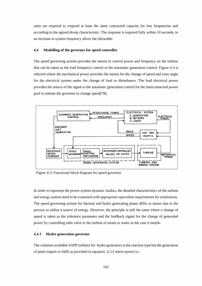
102

units are required to respond at least the same contracted capacity for low frequencies and

according to the agreed droop characteristic. The response is required fully within 10 seconds, to

an increase in system frequency above the allowable.

4.4 Modelling of the governor for speed controller

The speed governing system provides the means to control power and frequency on the turbine

that can be taken as the load frequency control or the automatic generation control. Figure 4-3 is

referred where the mechanical power provides the inertia for the change of speed and rotor angle

for the electrical system under the change of load or disturbance. The load electrical power

provides the source of the signal to the automatic generation control for the interconnected power

pool to initiate the governor to change speed[78].

In order to represent the power system dynamic studies, the detailed characteristics of the turbine

and energy system need to be examined with appropriate equivalent requirements for simulations.

The speed governing system for thermal and hydro generating plants differ in nature due to the

process to utilize a source of energy. However, the principle is still the same where a change of

speed is taken as the reference parameter and the feedback signal for the change of generated

power by controlling inlet valve to the turbine of steam or water as the case it maybe.

Hydro generation governor

The common available SAPP turbines for hydro generators is the reaction type but the generation

of plant require to fulfil as provided in equation (2.1) where power is:-

Figure 4-3: Functional block diagram for speed governor

103

P=9.81 η ρ Q H

In all hydro generation, governor requires water to flow in a column to impact the movement of

the shaft. It originates from the effects of water inertia diverted from a head with compressibility

to build for pressure in the penstock. The water hammering is due to water inertia on the guide

vanes to start to provide speed for the shaft. Figure 4-3 refers to the general arrangement of the

hydropower generation as in given in equation (2.1).

When carrying out dynamic studies, the hydraulic turbine transfer function includes the flow of

water in the water column for the generating plant. However, the following assumption is

considered:

a) The hydraulic resistance is negligible due to changes of load in the grid and governor

b) The penstock is inelastic and water is incompressible. The movement of water in the

column should be free to move without any diversions and leakage. The water should also

strictly move to provide the speed of the shaft with an unrestricted head and tail race.

c) The turbine output power is proportional to the product head as then provided in equation

(2.1)

d) The velocity of water varies directly with the gate opening and with the square root of the

net head

Therefore, the characteristics of turbine and penstock are determined by relating equations from

the above assumptions, However the assumption provide the rigid water column and

incompressible fluid as per basic hydrodynamic equations.

Figure 4-4: Typical water parts for hydro plant

104

Calculation of hydro-governor parameters

a) Velocity of water

The quantity of water depends on the water velocity, head, and the nozzle coefficient. It is also

restricted by natural flow of the stream, hence water velocity is determined by:

Where

V = Flow of water in meters3 per sec

G = Gate position

H = Hydraulic head

uK = a constant of proportionality- close to 0.98.

From the equation (4.69) it can be noted that the change of displacement will occur at operating

points when the gate position and the hydraulic head at the intake affects the operation of the flow

of water.

b) Turbine Power

The equation (2.1) provided in the literature review for hydropower generation where P=

9.81ηρQH is meant to maximize in the design. The turbine output flow relates and considers to

the built pressure and flow of water. It is represented as follows:

HVKP pm (4.70)

Where

mP = Turbine power output

pK = efficiency of the turbine usually 0.8 to 0.9 pu

H = Hydraulic head at the surge chamber

V = flow of water in meters per sec2

HGKV u (4.69)

105

From the equation (4.70), the basic variables for maximum generated power require effective

variations of the gate and flow of water.

c) Acceleration of water

The acceleration of water column due to change in head at the turbine is represented by newton

second law of motion, may be expressed as

HaA

dt

VdAL g

(4.71)

Where

= mass of density

L = Length of penstock

A = cross section area of the penstock

ga = acceleration of due to gravity (9.81m/s)

LA = mass of water in the conduit

Hag = incremental change in pressure at turbine gate

t = time in seconds

The acceleration of water column is calculated based on the characteristics of physics, the design

of the tunnel and pressure at the turbine. It is very difficult to determine the acceleration of water

and input for the development of its control system.

d) Water time constant

The water starting time is commonly referred to the acceleration time taken for water in the

penstock flow from intake to the turbine and in the case of available surge tank between the intake

and turbine. This then means also depends on the physical dimensions of the intake, penstock

and turbine inlet as can be noted in figure 4-4. The basic equation is

106

0

0

Ha

LVT

g

w (4.72)

Where

wT = Water time constant

L = Length of the penstock

0V = Initial velocity of water

ga = acceleration of gravity (9.81m/s2)

0H = Initial column of water at the intake

The water time constant wT varies with a load of the generator. The more water flow means the

more power output.

e) Turbine Gain

The amount of water flowing in the penstock depends on the gate position of the turbine. The gate

position normally is indicated as the percentage and also is varied through a potential resistance

to provide an indication to the system operator. Therefore the opening of the gates from no load

to full load can also be represented as equal to 1 per unit.

The turbine gain is calculated as follows

nlfl

tgg

A

1

(4.73)

Where

tA = Turbine gain

107

f lg = full load gate

nlg = No load gate

Hydro governor system model parameters

DIgSILENT provides the default hydro governor control parameters that require being calculated

for simulation studies. The detailed calculation methods for various parameters provided in the

section 4.2.3 can be termed as the essential data for a hydro plant station. It is believed that similar

values are used for the same type of governors on similar synchronous generators. In other ways,

the calculation of the hydro governors can be termed as steady state calculation parameters for

the input of the speed governor system. However, it is paramount to have knowledge of the type

of waterways that has been used for water flow in the penstock to run the turbines.

The requirement of the governor to be installed on the synchronous generators is to control speed

through water flow and load through the power transducer connected in the substation. It also

necessary to understand the requirements of governing hydraulic turbine through its physical

arrangement and dimensions. This will then provide a near behaviour of the interconnected

system during modelling simulation.

The operation of speed/load control function on the governor requires a feedback speed error to

control the gate position. In order to ensure satisfactory and stable operation of multiple power

generation from different generators in the interconnected system, the speed governor requires

having a droop characteristics. The purpose of the speed droop is to provide equal sharing between

the generating units. According to South Africa Grid Network Grid Code, it is set at about 4%

and it means the allowable speed deviation of 4% causes a 100% change in gate position and this

represent a turbine gain of 25%.

Table 4-1 presents the detailed parameters required for the speed governor. In the required

variables for the modelling of the governor, data is available at design study and inbuilt diagrams

for the generating plants. It can be observed that most rivers vary its water flow due to drought

and environmental degradation. It is essential for continuous monitoring of the water flow in order

to develop hydrological data and forecast the power generation capacity efficiency.

The required data for the hydro governor required as per table 4-1, need to have knowledge of the

physical design of the water tunnel for every power station. However, such data may not be shared

utility companies in SAPP and the data is considered as non-disclosure of information (NDI).

Equations (4.69- 4.73), provides the calculation of the required data for the hydro governor. It

108

requires knowing the head and flow of water. For the sake of analysis of power system

oscillations, the data has been sourced from different model designs provided in Powerfactory

software.

Table 4-1: Required parameters for the speed governor

Variable Units Description

rateP MW Rated Turbine Power

rateQ cc Rated Turbine Flow

rateH m Rated Turbine Head

rateG pu Gate Position at Rated Conditions

NLQ pu of Qrate No Load Flow

R pu Permanent Droop

r pu Temporary Droop

fT s Filter Time Constant

gT s Servo Time Constant

dbGov Hz Governor deadband

lakeH m Lake Head

tailH m Tail Head

lpen m Summation of penstock, scroll case and draft

tube lengths

aPen m2 Penstock cross section area

lTun m Summation of tunnel lengths to surge tank

aTun 1/m Tunnel cross section area

areSch m2 Surge Chamber Effective Cross Section

maxSch m Maximum Water Level in Surge Chamber

minSch m Minimum Water Level in Surge Chamber

109

4.5 Modelling of automatic voltage regulator

The automatic voltage regulator is also known as the excitation system is determined by

understanding the performance of the synchronous generator during the delivery of voltage to the

grid [79]. It is mainly installed to provide the direct current voltage source to field winding to

excite flux for the generator to initiate its generation. The dc voltage is the separate supply from

the battery for the operation and control of substation and associated equipment. It is required to

have the dc voltage in order to have a continuous supply and steady fast in operation of equipment.

Basically, most of the generators are the separately excited type that requires a dc supply to

provide a temporary magnetism to start running machines. The rotor is commonly a point where

most of the excitation voltage is connected to the generator. The excitation system will

automatically change over at the start of operation through the unit transformer of own machines.

After machines are synchronized into the grid the excitation will turn its function as the voltage

regulator for the generator.

The excitation system also responds to the grid disturbance so that the field winding provide

consistent voltage limits. It provides specified range of voltage so that the thermal limits should

be controlled in the generator to protect the rotor insulation due to high excitation voltage and

current from the field winding. The control of the temperature in the stator windings protects

excessive heating of the windings that cause damage to the insulation for the stator.

In power system, the excitation should effectively control voltage and respond rapidly to system

disturbance to enhance transient stability and effects small signal due to change of operational

level of the voltage and load in the system.

Types of excitation system [7, 8, 79]

The development of excitation control system on generators has been influenced by the

developments in solid state electronics. The development has changed the analog integrated

circuits with generators into digital technology where thyristors are used to provide power for the

excitation system. The control, protection and logic functions implement the analogue circuitry

by use of essential the digital components.

The change of technology in every aspect provides an advantage of being reliable, easy solutions

to the complex strategies analysis, friendly connection with other controls on the generator and

protection system for the generator.

110

The performance of the excitation control system depends on the characteristic of the excitation

system, generator, and power system. It is convenient to classify its dynamic performance and

achieve the required effectiveness responses.

From figure 4-5, the controller is the type of excitation used to perform the regulation of the

voltage. The controller processes the voltage difference from the grid as a feedback control and

sets the voltage of the excitation system. The power amplifier obtains source power from the grid

and at the start of the machine provides voltage field windings for the generator. The voltage will

be compared with the generated terminal voltage.

Based on the key characteristics of excitation system in figure 4-5, it is proper to identify and

define the required measurements in order to determine, evaluate and specify the performance of

the excitation control system.

The DIgSILENT library has provided the following types of excitation and it depends on

knowledge of the status of the generators in the SAPP grid. The status of each generator requires

knowing the history of normal rehabilitation and at a particular moment it will be able to predict

the type of excitation system. The type of the excitation system used in the simulation has an

effect on the fast response of voltage control. Therefore the effects of excitation on stability both

in transient and dynamic modes of operation. In a literature review, it was learned that the change

of terminal voltage to acceptable values will provide the ability to transfer the synchronizing

coefficient power within the shortest time.

DC Excitation System

These type of excitation is becoming extinct and were used in the early invention of the

synchronous generators. The principle of voltage regulation was to use the magnetic and rotating

amplifiers for the ac excitation system [80]

Figure 4-5: Functional block for automatic voltage regulator

111

It used the dc generators as a source of excitation power and provide current to the rotor of the

synchronous machine through slip rings. The exciter was driven by a shaft of the generator or

motor. The amplidyne was used as separately excited, the exciter field consisted of a permanent

magnet as a pilot exciter. The amplidyne is a special type of the general class of rotating

amplifier[80].

The controller achieved the voltage measurement through the slip rings of the generator, tE which

is used to regulate the required voltage in reference to the grid. However, the excitation was

controlled through the use of amplidyne a form of the rotating amplifier for automatic supply of

voltage to the generator terminal. The adjustment of field rheostat was to operate as a manual

control of the exciter field in case of fault amplidyne or out of service.

AC Excitation System 6

These type of excitation system replaced the DC excitation due to technology change for

performance improvement.

The alternators use the same ac of the synchronous machines and the exciter is connected to shaft

of the same the turbine generator. The output of the ac in the exciter figure 4-5 is rectified by

either automatically or manually to produce the required dc voltage for the generator field

winding. The dc field requirement is produced by use of the ac alternator and by either rotating

or stationary rectifiers.

On stationary rectifier, the characteristics of the thyristor are normally used to regulate the

voltage. The conducting of the thyristors by firing a voltage provides self-excitation from the

exciter alternator and uses an independent static voltage regulator to maintain its output voltage.

In normal circumstances, there are two main operating modes to compliment the functions of the

excitation system. The ac regulator automatically maintains the generated voltage from set limits

of ac voltage on the regulator. The dc regulator acts as the backup, station dc supplies are available

for operation and control of the generator. The dc supply will be inverted to provide the ac supply

for the field armature.

Unlike the DC rotating rectifier, the AC rotating rectifier obtains and controls the voltage source

whilst in motion. The rotating rectifiers supply the dc voltage directly to the generator field

windings. However, the rotating structure comprises of the armature windings, permanent

magnet rotor, and a rectifier connected in series in order to maintain the voltage at the generator

terminal. The rotating structure moves with field windings and is supplied from a stationary field.

The voltage regulator controls the voltage from the stationary field that supplies the ac exciter and

112

when it is rotating maintains the armature voltage at the terminal of the generator. This type of

rectifier does not require the manual operations, it is self-excitation.

Static Excitation System

An improved design of the AC excitation system has similar functions of the stationary rectifier

but this type has a static rectifier different from the rotating rectifier. It provides virtually the same

excitation character performance. The other difference worth noting is the source of power supply

to the rectifiers. The AC excitation uses the line drop compensator to measure the voltage drop

from the current and voltage transformers on the generated voltage. The AC excitation measures

and validates the impedance of the system to regulate the on the reference voltage and acts as the

feedback control as shown in figure 4-5.

The static excitation, therefore, uses supply from the unit transformer on the three phase, 400V

from the LV side of the voltage at the generator transformer, the generator voltage at the generated

rate and stationary dc supply.

The operation of the synchronous generator requires the excitation system to initiate the start of

the machine. The generator requires the field winding to have a field current so that the magnetic

excites the machine to start rotating and generate a voltage. The station dc supply momentarily

provides the voltage supply to the field windings in order the generator to start generating voltage

and the process to build up field flux in the generator is called the field flashing.

Voltage –Source Controlled rectifier

It is connected to the same generated voltage of the synchronous machine and also depends on

the own generated voltage.

When the system experiences a fault condition, it stresses the generator terminal voltage due to

the very small inherited time constant. The only drawback on the voltage source controlled

rectifier is mainly the offsetting by its virtually instantaneous response and high post-fault field

forcing capability and recommended for interconnected power systems such as SAPP grid [81,

82]. Despite the voltage source controlled rectifier takes time to respond when regulating already

high voltage.

Compound-source rectifier system

This type of static excitation can be taken as the self-excitation of the synchronous generator. The

generator terminal provides the source of voltage to the exciter contrary to the rest of the

113

excitation system that takes supply from the slip rings of the shaft. The basic feedback provision

is controlled by saturable reactors that control both ac output and exciter values. This type of

excitation system was originally designed for the smaller units of the generator[83] .

In cases where this type of self-excitation system is generating low ac output voltage and

concurrently the exciter needs to correct the low voltage. The line drop compensation then

regulates the voltage. The line drop compensation simulates the voltage drop through the current

and voltage transformers in the grid. The current transformer is installed on neutral earth of the

common stator windings of the synchronous generator.

This neutral current transformer provides also a continuous path to ground of the generator. If it

is open then the main protection of the generator fails operation due to broken conduction to the

ground. However in the case of faults then the current transformer will saturate such that any

increase of voltage, current remains unchanged. This means that the line drop compensation

provides the control of voltage for the generator. The current transformer is connected to the star

points of the stator windings to the ground and outside the zones for differential protection.

Compound –controlled rectifier excitation system

This system functions with controlled rectifiers in the output of the exciter circuit. The voltage

and the current derived sources from the excitation transformer are installed together with the

generator stator to provide the source of supply to the excitation control system. This then results

in a fast response on faults on the excitation to prevent causing damage to the stator.

The three phase supply from the generator stator windings provides a voltage supply to the

excitation. The primary side of the excitation transformer also supplies the voltage transformer in

the stator windings which is connected in the series linear reactor. The voltage supply through the

slip rings supplies the excitation control composed of the rectifier and thyristors.

The voltage and current sources provide power to the rectifier and thyristors that regulate the

voltage for the generator. Moreover, the linear reactor acts as in such manner as a compound the

normal behaviour of the excitation system and also reduce fault current into the generator.

114

CHAPTER 5

SIMULATION OF RESULTS

5.1 Methodology and Simulation results of SAPP grid

The simulation of the SAPP grid was carried out to determine the power oscillation of the region

from the synchronous generators hence the rotor speed has been used to obtain the frequency

deviation of the network[84] . DIgSILENT Powerfactory uses the rotor equivalent circuits

diagram on synchronous generator using electromagnetic transients and modal analysis to obtain

the behaviour of the power oscillation and the frequency stability The required data and circuit

are shown in Appendix B -1 and B-3.

Rotor angle and frequency behaviour on synchronous generators

In order to determine the rotor behaviour on change of sudden drop of load, load flow analysis

was carried out on the transmission line to be switched off in order to transfer that particular load

to alternative transmission line. The transfer of load helps customers to have supply at all times

during the maintenance [84] . However the rotor behaviour under fault condition will be initiated

with a fault without carrying out load transfers.

(a) Initiated a sudden load drop to switch of the transmission line between T1_6 and sub 22:

This point was selected because the transmission line is a radial feeder and has no alternative

transmission line to supply the north and east blocks. First of all, determined the normal load

flow from the thermal plant to sub 22 .Then at sub 22, determined the branch load flow, a

small load was supplying sub 21 and the rest was the inter power exchange to East block

through sub 23.

The equivalent load that was supplying to the east block from sub 23 was transferred to

increase the generation at T3-1 and T2-6 .Then switched off the 400kV line between sub 23

and T2_6 and thereafter switched the line between T1_6 and sub 22. It means that the only

sub23 was affected with this simulation.

Figure 5-1 indicates that the load switching caused the change of frequency to oscillate

between acceptable frequencies of 50.5 Hz and 49.957 Hz within 6.066 s on the first swing of

frequency. The second swing of the frequency settled at 50.320 Hz before settling above 50.1

Hz. The first swing was the action being conducted in the speed governor temporary droop

115

that was set at 0.5 s. The second swing is caused by the turbine control to increase mechanical

power due to lack sufficient electrical power that was switched off on Sub 23 then the

frequency settles above 50.01 Hz. Figure 5-1 was obtained on frequency vs time for

synchronous generators in the modified SAPP grid.

Figure 5-2: Rotor effects due to change of load in SAPP grid

Figure 5-1: Frequency deviations after change of load in SAPP grid

116

Figure 5-2 represents rotor angle versus time. The two generators T1_6 and T1_3 had 152 degrees

higher than the rest of the synchronous generator plotted in the figure. It can been seen from the

figure that T1_6 had another swing at about 8s. It is at the same time the frequency had the second

swing before settling at 77 degrees. The decrease of rotor angle has influenced the frequency of

the system to increase due to turbine controls and when the rotor angle stabilized the frequency

too becomes constant.

It is clear from the Figure 5-1 and Figure 5-2 that rotor angle influences the change of frequency

and also the cause the system to operate within a band of frequency. It has been also observed

that the change of load can influence the rotor behaviour to change too. The load change has

caused unstable condition of synchronous generators to oscillate but remain in synchronism.

(b) Initiated a sudden switching on a hydro generation plant at H1_6

An equivalent load of 150 MW was switched off in west block of the modelled SAPP grid.

Figure 5-3: Frequency deviations of a general fault on generator H1_6

117

Figure 5-3 indicates that the frequency dropped in the synchronous generators modelled in SAPP

grid due to switching off generator but remained in synchronism despite large machine oscillating

within the frequency band. Even though the frequency in figure 5-3 dropped but remained within

the acceptable band of 50.011 Hz and 49.191 Hz. The network also fails to settle back to 50 Hz

but swings around 49.836 Hz. Unlike the results on the switching of the transmission line, the

generating stations have uniformed dropped the frequency. The effect of 150 MW machine has

caused 665 MW more damping than the rest of the generators.

Similarly to Figure 5-2, the rotor angle drops as shown in Figure 5-4 when one machine was

switched off the circuit, the rotor angle drops tremendously, Figure 5-4 indicates rotor angle for

the generators decreasing due to fault on H1_6 and the change has considerably changed the

turbine power and also sudden drop of load for the system.

From the same figure 5-4, T2_6 has not been affected by the fault because the rotor angle is

relatively at normal operation and this the reason why it was oscillating with the frequency of the

rest of the generators in figure 5-3

Figure 5-4: Rotor angle effects of a general fault on H1_6 generator

118

(c) Initiated fault between T2_6 and sub 31 in the eastern block

The substation is fed with the longest transmission from the generating station and also furthest

point from the grid.

Figure 5-5, indicates three bands of frequency deviations caused by the fault between T2_6 and

sub 31 transmission line. T2_6 is oscillating between 50.680 Hz and 49.626 Hz from 36 s. T1_6

oscillates between 50.404 Hz and 49.859 Hz and also hydro generators within the 50 Hz. The

overall frequency deviation for the grid due to fault on the transmission line has caused the

increase of system frequency due to loss of load in the network. T2_6 oscillates highest frequency

because it is directly affected with the fault.

Figure 5-6, depicts the rotor angle having three distinct operating angles affected by the fault due

to fault on the transmission line between T2-6 and sub 31.

Figure 5-5: Frequency deviations of 3phase fault between T2_6 and Sub 31

119

The oscillation of the rotor angle has caused from the small generators to respond to unknown

oscillations that have not affected their system. Form the various simulations T1_6 generators

exceeds the rest of the generators in damping oscillations.

From Figure 5-1 to figure 5-6, they have depicted that the change of load angle affects the rotor

movement and also responds to the turbine control to produce the required mechanical power.

However, speed is the most essential component that the mechanical power should respond

effectively due to changes on the electrical power. The change of electrical power vary due to

load variation in the power system grid but at the same time the grid require to maintain the

frequency. Primarily, the control of frequency is achieved by controlling the mechanical power

through the speed – governor system and require precise measurement to achieve the required

control of the generator.

Simulations of faults using electromagnetic transients of the turbine

(a) A three phase fault was initiated between T1_6 and Sub 22 on transmission line and without

any load transfers:

Figure 5-6: Rotor effects due to 3phase fault between T2_6 and Sub 31

120

This point was selected for initiation of a fault because most of the simulation results

indicated high rotor angle and speed. The fault was initiated in the electromagnet transient

analysis in the Powerfactory tool to check the turbine output.

Figure 5-7 depicts two frequency bands, the higher frequency is over 53 Hz within 1.2 seconds

from the small rated generators in the west and central blocks .and the large generators at T2_6

generating station controlled the frequency within the same time. The west block experiences a

disturbance from external grid and the system operator will not realise the sudden over frequency

that occurred in their network. The sudden change of frequency in the west and east will have no

protection relay operations to indicate the nature of fault

The point of fault is the interconnecting point between the other blocks with the eastern block

which has the largest machines for the network. From figure 5-7 it depicts that the whole of the

generation plants in the west and central had tripped due to over frequency because the fault was

operating beyond 51 Hz the statutory requirements.

The output power has been affected by the fault as shown in figure 5-8 and as a result of over

frequency that has separated the grid into two isolated islands as shown in figure 5-7. This can be

noted in figure 5-8 where only a single plot is flowing close to 1.00 pu when all the machines

have collapsed in the system

Figure 5-7: Frequency deviations of a 3phase fault between T1_6 and Sub 22

121

The turbine power of each generating station differs due to design of the plant and also the share

of power dispatch distributed amongst the generators. Therefore the large machine will be shared

with the larger amount of power to generate than the machines with small capacity.

(b) Initiated a fault on the transmission line between Sub 29 and 31

A simulation was initiated on the transmission line between Sub 29 and Sub 31 to determine

the effects of fault at the furthest point of the SAPP grid can supply load and to represent the

longest overhead line to Sub 31 in east block.

Figure 5-9 shows that the all synchronous generators are swinging above the normal

frequency at about 50.1 Hz except TH 2_4 which is oscillating at high frequency and the

damping is ever increasing as from 11 s. This fault has a direct effect on generation of T2_6

and the loss of 354 MW brings a high frequency deviation for the plant. Hence, the oscillation

of the large machine has caused the other generators to oscillate due to the impact caused by

the fault on the line. If the oscillations continues, the frequency control will start loading

shedding other loads. The system operators from the central and west will not know the cause

of the load shedding in their system

Figure 5-8: Turbine power fluctuations due to a 3phase fault between T1_6 and Sub22

122

.

The generator HPP3-1 at H3-6 generating station in figure 5-9 and also in figure 5-10 started

to separate from the system but then become synchronised in frequency with the other

generator in central and west blocks. The generator HPSP4-3 is operating at considerably

low power output as compared with the other generators and this is due to its contribution in

power output in the grid.

Figure 5-9: Frequency deviations of a 3phase fault between Sub 29 and sub 31

Figure 5-10: Turbine power fluctuations due to a 3phase fault between Sub 29 and Sub 31

123

The voltage output from generator T1-6 is showing higher values than the rest in the network

from figure 5-11. The results has been caused by the high load angle emanating from the

generation plant and was due to synchronizing coefficient power to sustain the electrical

power

(c) Initiated a fault on the transmission line from the west block network:

The west block main transmission lines have been provided with adequate alternative

transfer of power and hence have sufficient capacity of the transmission line. The fault was

initiated from transmission line between sub 7 and sub 8.

Figure 5-11: Voltage variations due to a 3 phase fault between Sub 29 and Sub 31

124

Figure 5-12 indicates that the frequency deviations on synchronous generators caused by a fault

between Sub 7 and Sub 8 in the west block. The fault has caused the frequency to rise and the

speed governor also controlled within 2 s but the oscillation for different generating station kept

oscillating within the frequency band. The large machine has the high order of oscillation than

the rest of the synchronous generator when affected by fault.

Figure 5-12: Frequency deviations due to a fault between Sub 7 and Sub 8

Figure 5-13: Rotor angle effects due to a 3 phase fault between Sub 7 and Sub 8

125

From figure 5-13, the rotor angle of THPP1_6 has dominated oscillating higher than the rest of

the synchronous generators. The hydro generators seem to oscillate together when affected by a

three phase fault between Sub 7 and Sub 8.

When a rotor has been operating at very low angle in the synchronised power system, it will cause

high frequency oscillation and this has been observed with generators having large capacity in the

network. This has been noted throughout the simulations on the rotor angle for the interconnected

power system.

Figure 5-14 shows that the voltage are operating at high values at the generating plant at T1-6

whilst the rest busbar are operating with the acceptable limits.

Figure 5-14: Voltage variations due to a fault between Sub 7 and Sub 8

126

Modal Analysis for SAPP grid

Modal analysis in the Powerfactory tool uses the eigenvalue and eigenvectors to determine the

frequency oscillations.

In the figures 5-1 to 5-14, the plots have shown that the frequency and rotor angle for the

synchronous generator oscillate when a fault and switching has occurred in the power system.

The synchronous generators and the controllers such as automatic voltage regulator and governor

have been used to determine the complex frequency of the system

(a) Initiated a calculation of eigenvalue using the Arnoldi/Lanczos method[7, 49]

The method has determined the natural critical system oscillation for the frequency at 1 Hz

an equivalent of 6.28 radians per second.

Figure 5-14 has been tabulated with its details in Table 5-1. The coordinates in the complex

plane denotes the stability of the grid because they are all in the left hand side and the real

parts are all negative.

Table 5-1 shows the mode values and details obtained from the eigenvalue plot in figure 5-15

and it can be observed that the damping time constant on mode 00001 and mode 0002 have higher

time constant than the rest of the modes. It is the obliged to work on the time constant in order to

improve the stability of the grid. However it is required to analyse the two modes that can be

termed as the interplant mode oscillations occurring in the SAPP grid. The two modes have been

tagged as 0001 and 0002 in figure 5-15.

Name Real part Imaginary partMagnitude Angle

Damped

Frequency Period Damping

Damping

Ratio

Damping

Time Const.

Ratio

A1/A2

1/s rad/s 1/s deg Hz s 1/s s

Mode 00001 -0.1136 5.8830 5.8841 91.1065 0.9363 1.0680 0.1136 0.0193 8.8004 1.1290

Mode 00002 -0.0353 6.8197 6.8198 90.2964 1.0854 0.9213 0.0353 0.0052 28.3470 1.0330

Mode 00003 -0.5708 7.0253 7.0484 94.6451 1.1181 0.8944 0.5708 0.0810 1.7519 1.6661

Mode 00004 -0.7842 7.4507 7.4919 96.0087 1.1858 0.8433 0.7842 0.1047 1.2751 1.9374

Mode 00005 -0.5487 8.0274 8.0462 93.9105 1.2776 0.7827 0.5487 0.0682 1.8224 1.5365

Mode 00006 -1.4560 8.6346 8.7565 99.5715 1.3742 0.7277 1.4560 0.1663 0.6868 2.8850

Mode 00007 -0.8590 8.9280 8.9692 95.4956 1.4209 0.7038 0.8590 0.0958 1.1642 1.8304

Mode 00008 -0.8590 8.9280 8.9692 95.4956 1.4209 0.7038 0.8590 0.0958 1.1642 1.8304

Table 5-1: Values for critical frequencies in the eigenvalue plot

127

Each and every critical coordinates plotted in the eigenvalue have the controllability and

observability of the modelled controllers in the synchronous generators. The controllers that are

shown in figure 5-16 on the right hand side are termed as the controllability that will impact on

the oscillations for SAPP grid. These are the synchronous speed controllers that are causing the

instability during the simulations on the electromagnetic transients and require to be controlled

for effective operation of the grid. It can be observed that the generator THPP 1_6 has a speed

problem and showing a high value.

From figure 5-16, it indicates that the rotor speed is causing the instability of the system and it’s

the thermal plant station problem

0002

0002

0002

0002

0002

0002

0002

0002

0002

0002

0002

0002

0002

0002

0002

0002

0002

0002

0002

0002

0002

0002

0002

0002

0002

0002

0001

0001

0001

0001

0001

0001

0001

0001

0001

0001

0001

0001

0001

0001

0001

0001

0001

0001

0001

0001

0001

0001

0001

Figure 5-15: Critical frequencies obtained for the modelled SAPP grid

Mode 0002

Mode 0001

128

From figure 5-17 shows that the voltage control requires further settings on gain and time

constants for the automatic voltage controller in the excitation system than the available settings

in the synchronous generator. The indication to plot the requirement of the settings in the

eigenvalue plot is termed as the observability of the system. The settings on the gain of the

automatic voltage regulator does not suffice the eigenvectors to control the voltage and this is the

reason the generator was experiencing rapid changes of voltage in figure 5-14. In order to change

the gain, it was required to under the behaviour of the type of excitation and the circuit

components whether can withstand high amplification of the voltage. The observability acts the

elements that have been noted during the control of the system to correct the instability

experienced in the system

Figure 5-16: Controllability determined from mode 0001

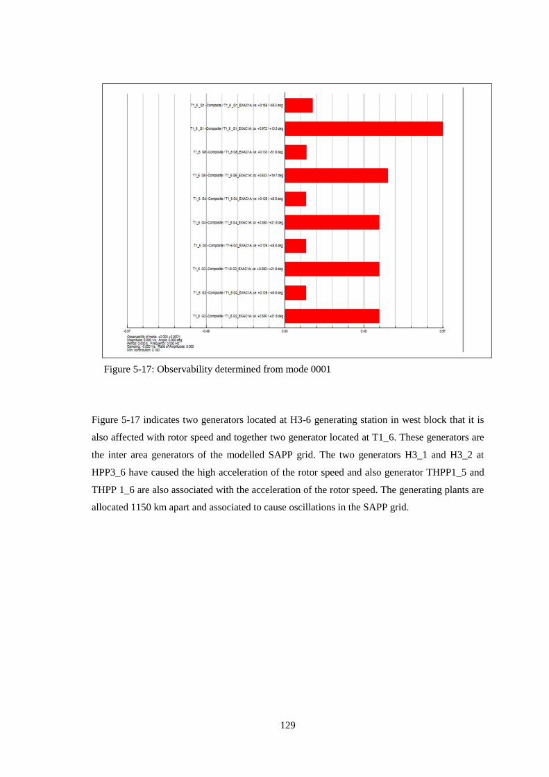
129

Figure 5-17 indicates two generators located at H3-6 generating station in west block that it is

also affected with rotor speed and together two generator located at T1_6. These generators are

the inter area generators of the modelled SAPP grid. The two generators H3_1 and H3_2 at

HPP3_6 have caused the high acceleration of the rotor speed and also generator THPP1_5 and

THPP 1_6 are also associated with the acceleration of the rotor speed. The generating plants are

allocated 1150 km apart and associated to cause oscillations in the SAPP grid.

Figure 5-17: Observability determined from mode 0001

130

Figure 5-18: Controllability determined from mode 002

Figure 5-19: Observability determined from mode 0002

131

From the figures 5-15 to 5-19, it can be concluded that most of the generator will operate under

steady state in SAPP grid but it is required to further improve on the gain of excitation system.

This also means in practice that under fault conditions the oscillation will affect the Zambian and

Zimbabwean power networks due the inter area oscillations between T1_6 in Zimbabwe and

H3_6 an IPP in Zambia

Methods to improve rotor speed in synchronous generators

There are three ways to improve the speed of the machines at TH1_6 apart from the site location

of the generating plant. It should be borne in mind that the plant is located at a site 355km away

from the load centres and the transmission line should require voltage compensators at both ends.

The two sides are from T1-6 to sub 22 and also from T1_6 to sub 17.The effects of speed has

occurred due to the following:-

a) The speed in the model is derived from the flux of the generator on d and q axis of the

synchronous machines and by changing the parameters of the inductance and resistance

rotor speed will improve in simulation. The change of parameters would best suit when

designing a newly generation plants and not on the already existing generation system.

b) Additional torque being applied to the generator to increase the moment of inertia and it

will be appropriate on the simulation for the new design of the generator and on the existing

generator requires increase of weight to the rotating parts of the generator. The additional

torque can be applied to a large generators by installing a sub resonance on the busbar

before transfer of loads to different substations so that the effects of the high damping

oscillations caused by the large machine is eliminated in the oscillations

c) The change of gain and time constant in the excitation has changed the speed of the rotor

on the existing generators like SAPP grid and it all depends on the circuitry technology and

type of excitation system applied to the generator. Hence, the observability that have been

noted in figures 5-17 and 5-19 have indicated the need to adequately tune the excitation

system. There are different methods to tune the excitation in order to increase the gain such

as the installation of power system stabiliser in the synchronous generator and static Var

compensators that are determined in the contingency analysis study.

132

CHAPTER 6

DISCUSSIONS ON THE DYNAMIC PERFORMANCE OF SAPP GRID

The steady state analysis for the synchronous generators, transmission overhead lines, load

behaviour and mathematical fundamentals are relative to the study of dynamic performance of

the modelled SAPP grid. The exigencies explained in the steady state has led to various studies

of power network to analyse performance and behaviour of the power system so that the reliability

and quality of supply was continuously prevailing at all times. The simulation of any power

networks are derived from the mathematical analysis and developed into a DIgSILENT

Powerfactory software. It was for this reason the load flow of the SAPP was modelled to obtain

the grid adequacy of power transfer and to be used for the evaluation of generated power to run

for dynamic studies.

The dynamic analysis involves on the electromagnet transient analysis in the nodal equation and

eigenvalue in the modal analysis to determine time based and frequency oscillations as the

required character for the study. The study analyses the effects of synchronous generator and its

associated speed governor and automatic voltage regulator on the system stability and

performance on the interconnected power system. The synchronous generator plays an important

role in the interconnected power system to provide supply unlike any other components in the

power system network. It is for this reason that the undertaken study would want to understand

the behaviour of the excitation and speed control in SAPP grid. The results of the electromagnet

transient provide the behaviour of the network in a waveform and the modal analysis will provide

details in the complex frequency mode. The eigenvalue plot provides the character of the

frequency and how the mode was achieved by checking the elements of the speed controller and

automatic voltage regulator. Presently, the details provided by the modal analysis are not

monitored in the power system and such interactive indication can improve the performance of

the power system.

In the simulated results, the figures 4-6 to 4-19 have been plotted to indicate the behaviour of the

rotor angle, speed relative to frequency and voltage in damping oscillations. In the time based

plots, it is very difficult to determine the actual frequency amplitude or actual measured frequency

and only provides the kind of behaviour being experienced during the fault. The figure 4-20

provide the critical frequencies associated in the system performance and each stable cross will

show the character and the corresponding equipment as shown in figures 4-21 to 4-24.

133

6.1 Discussions on simulated results

The plots obtained during simulations have shown that the faults and switchings in the

interconnected power system respond to the effects of the fault and have returned after controls

to remains in synchronism hence creating another operating value. When the synchronous

generators have been affected by a disturbance, the frequency of the system was oscillating due

to changes of the operating rotor angle in the synchronous machines. The SAPP grid simulated is

affected by the rotor angle speed at TH1_6 and H3_6 and every simulation the rotor speeds were

higher than expected operations.

The SAPP grid in figures 4-12 and 4-13 after initiating a fault between T1_6 and sub 22 ,the

simulation showed two distinct separations of the system due to interaction of large generators

located at T2_6 and the rest of the generators located in the central and west blocks. The effects

of the separated system has likely been caused the generators in the west and central block to

initiate frequency change and cause load shedding due to frequency increase or decrease beyond

the acceptable regulatory requirements. The large generators in SAPP has a higher control area

frequency bias at a rated MW/0.1 Hz than the rest of the generators. This frequency bias causes

also the damping oscillation between the large and small generators where the former would

possibly control to match with the rest of the generators to remain separated.

The simulation of eigenvalue plot, the Arnoldi/Lanczos method was selected in the Powerfactory

tool to identify the most critical modes of interarea oscillations in the SAPP grid[49]. The critical

frequencies are normally located in the range of 0.2 to 1.0 Hz because the low frequency is rated

at such rate. It has been shown that there is an inter area oscillations between T1_6 and H3_6 as

shown in the observability of mode 0001 and mode 002 in respect to speed and voltage control.

The generating stations are located in different countries and over thousand kilometres away.

It should also be known that in a large network such as the modelled SAPP grid more especially

when run on the electromagnetic transient analysis, there shall be two separate interarea

oscillations [7] that may occur such as

(a) A very low frequency (0.1 to 0.2 Hz) that has occured on all generators in the power system.

It has been identified in the plots that the large generators from South Africa have been

swinging against the rest of the generators connected in the system.

(b) A high frequency in the range (0.4 to 0.7 Hz) the generators also swinging amongst each

other within the same frequency just like figure 4-14

134

The nature of separation into two area oscillations just like that has occurred in figures 4-12 and

4-14, the system operators on the west block will experience a sudden frequency rise and the

effects of automatic load shedding will be initiated to cause trip without realising that the fault is

beyond their own control area and east block will too realise abrupt rise of frequency and

stabilising without actually knowing the cause of such incidents.

The power monitoring instruments do not provide an immediate indication to show oscillation of

frequency due to slow sampling rate of SCADA by use of transducer. The values shown in Table

4-2 for the critical frequencies in the modelled SAPP may not be obtained from SCADA because

it has a slow response to data acquisition at 1 sample per 4-10 seconds. From the NERSA grid

code requirements, the allowable time for the full operation of the governor is 10 seconds and due

to slowness of data acquired from the monitoring device the effects of change of speed could not

be noticed by the system operators.

There is a disparity of error on measurement that occurs between the input supply of the excitation

system and speed governor on the generator. The difference can affect the rotor angle in practice,

the excitation obtains the input source of voltage direct from the secondary output of voltage

transformer and the speed governor obtains the load input from the output of power transducer

both from the grid. This means that the requirement to change the voltage has depended on the

instantaneous value of the grid and the same voltage becomes one of the input to the power

transducer. The change of voltage to the power transducer has not effectively changed its output

for the speed governor signal because of the due process to convert the inputs to dc current and

caused a delay to control the speed. Therefore, the excitation require to improve its control of

voltage to improve stability of the power system.

The SAPP grid was intended for the supply of own use by the participating members and it can

be visibly seen from the modelled network that the synchronous generators supply the electricity

in an adequately designed transmission lines. The west block is meant to be the network of Zambia

and the generation plants are located in the south of the country to supply the load centres the

mining centres in the north of the country. The central block is the network for Zimbabwe. The

thermal generating plant T1_6 is located in Zimbabwe and the site runs very long transmission

line to load centres over 355km. The behaviour of the rotor speed noted during simulation befits

on the character to suffice the synchronising coefficient power due to the line capacitance and

reactance required for the load.

135

CHAPTER 6

CONCLUSIONS AND RECOMMENDATIONS

The dynamic analysis of SAPP grid has produced the power oscillation that has been characterised

with low frequency caused by synchronous generator in an interconnected power system. The

behaviour of the generator depends on the nature of disturbance and magnitude of the disturbance

to remain in synchronism. The character of the excitation system to regulate voltage limits and

the speed governor to control the rotor shaft speed initiated the power oscillation in the

interconnected power system. When the voltage was being controlled, changed the rotor speed to

match the grid frequency.

The SAPP grid was modelled in the DIgSILENT Powerfactory to simulate different types of

power system analysis amongst the load power flow and the modal analysis The SAPP grid

modelled consists of the transmission line from Zambia, Zimbabwe, Botswana and part of South

Africa and the associated synchronous generators that has been used to demonstrate the low

frequency oscillation in the Dynamic Analysis of SAPP network. The modal together with

electromagnetic transients (EMT) analysis were used to simulate in the software to generate the

frequency oscillation and time based plots to determine the required dynamic behaviour of the

SAPP grid. The modal analysis produced the bar graph and the modes to be evaluated for the

power oscillations .The left eigenvectors in the bar graph demonstrated the parameters that have

provided stable variables during simulation on load flow and the right eigenvectors provided the

parameters that were unstable during operation. It was from the electromagnet transient analysis

that provided the damping oscillations of the rotor and frequency relative to rotor speed. However,

the behaviour of the modelled synchronous generators have shown the interarea damping

oscillation from different area of operations. The Arnoldi/Lanczos method was used to identify

the critical oscillations in SAPP grid in the complex frequency of the eigenvalue plot. The inter

area oscillation was identified based on the results that indicated very high time constant of the

eigenvalue plot from the calculation of Arnoldi/Lanczos method in Powerfactory tool.

In the electromagnetic transient analysis, it has been observed the frequency of the synchronous

generators decouples between large and small generators in the SAPP grid under the fault

conditions. If the fault was located in the area of large machines the small machines would over

accelerate and cause over frequency then an eminent to load shedding of the part of the system to

remain in synchronism. If the fault occurs in the area of the small machines, the large machine

has been oscillating conspicuous within the same frequency band.

136

It was therefore to noteworthy to understand that the critical oscillation that was demonstrated in

simulation can be re-tuned to increase the excitation gain incorporated with a separate controlling

unit of power system stabilise to the synchronous generator. The power system stabiliser has

reduced the damping oscillation considerably and improve reliability of the power network. The

originality of power stability is based at the generating plant and during the study of the dynamic

analysis the line compensators are neglected.

Further to the power system stabiliser, the modern power system monitoring measurements is

based on the synchro phasors measuring unit to be installed at strategic substations in order to

(a) Improve system monitoring due to sampling rate of data to be analysed by the instrument

(b) Provide valid system parameters on-line for the system operators to be aware of the

dynamic changes of the system

(c) Provide technical audit data required for regulatory performance indices on transmission

and generation plant.

(d) Provide event record due to disturbance and switching

(e) Provide the effective planning actual data from the network

Presently the synchro phasors are not available in SAPP network, but if they are available are not

being fully utilised for the effectiveness and usefulness in providing the necessary requirements

of power system. The availability of such instruments would be used to verify the simulation

results with the actual results of the system under study in SAPP grid.

The dynamic performance in the modelled SAPP grid has been affected by the

performance of the synchronous generators when under any disturbance due to:-

(a) The behaviour of large generators towards the small generating plants:

It has been observed that under any disturbance the large generator has a high

oscillations within the system synchronism. However, depending on the severity of

the oscillations and location of the system may collapse.

(b) The existence of the natural transmission line link:

SAPP network has a natural transmission weak link that connects between Zimbabwe

and South Africa. There is no alternative route of transmission line to transfer power

from Zambia and Zimbabwe to supply South Africa or vice versa. Therefore the

bottleneck situation impedes the power trading between the mentioned countries. It

137

has observed in the simulations to be the epic of inter area oscillation around the

generating station connect the link.

(c) Hydro speed governor effects on the impact of environmental impact:

In case of hydro generators where its speed governor depends on the restricted water

canal movement, any natural changes in the flow of water to run the machine would

affect the performance of the generators. It is imperative for such countries to

constantly study the behaviour of its source of energy.

It has been then required for the SAPP members to undertake the study of power

oscillations in their perspective countries and also the whole network. This will depend

on acquiring performance data at points of common connection and also invest in

acquiring the wide area monitoring system. The instruments provide adequate real time

data for planning and system operations to likely monitor the dynamic performances of

the power system network. The mitigation factors for power oscillations require adequate

data on power parameters at the point of connection that has been monitored

continuously.

The electricity regulatory body require to encourage the power utilities company to

provide own telecommunication link to strengthen the acquiring of power system data

and quick response on operations of equipment in SAPP network. The high speed data

transfer will effectively provide smart grid operation and includes monitoring systems.

The electricity regulatory body need also to enforce the harmonisation of standards and

operations of SAPP with emerging technology for optimal technical and economic

performances.

7.1 Recommendations

After identifying that the focal points of power oscillations in SAPP, it would be required to verify

with real time measurements of the load flow and behaviour of the voltages under normal

operations of the power network. Hence, the need for phase measurement unit to ably measure

the voltage angles at the strategic substation. Then the measured data will assist to re-tune the

control system of the automatic voltage regulator of synchronous generators to provide high gain

and adequately control damping oscillations in SAPP grid.

138

REFERENCES

[1] S. J. T. Mwale and I. E. Davidson, "A Steady-State Contingency Analysis of the SADC Regional Grid Using the N-1 Criterion," Journal of Energy and Power Engineering 9, pp. 479-485, 2015.

[2] G. Thornton, "2015 SAPP Annual Report," Harare , Zimbabwe2015. [3] L. Musaba, "The development of the SAPP competitive electricity market," in 2005 IEEE

Power Engineering Society Inaugural Conference and Exposition in Africa, 2005, pp. 188-194.

[4] S. J. T. Mwale and I. E. Davidson, "Security Analysis of the SADC Regional Regional Electric Power Grid Using DIgSILENT Powerfactory Software Tool," Eskom Power Plant Engineering Institute Student Conference, 5 & 6 May 2014 2014.

[5] P. Naidoo, L. Musaba, W. Balet, and A. Chikova, "Towards developing a competitive market for regional electricity cross border trading: the case of the Southern African power pool," in Power Engineering Society General Meeting, 2004. IEEE, 2004, pp. 1377-1384 Vol.2.

[6] K. R. Padiyar, Power System Dynamics Stability and Control, Second ed.: BS Publications, 2008.

[7] P. Kundur, Power System Stability and Control. NewYork: Mc Graw- Hill, 1994. [8] P. M. Anderson and A. A. Fouad, Power System Control and Stability, Second Edition ed.

IEEE Press: John Wiley & Sons, 2003. [9] P. Kundur, J. Paserba, and V. Ajjarapu, "Definition and classification of power system

stability IEEE/CIGRE joint task force on stability terms and definitions," … on Power Systems, 2004.

[10] G. Shackshaft, "Effect of oscillatory torques on the movement of generator rotors," Electrical Engineers, Proceedings of the Institution of, vol. 117, pp. 1969-1974, 1970.

[11] R. G. C. Secretariat. (2014). http://www.nersa.org.za/Admin/Document/Editor/file/Electricity/IndustryStandards/SAGC%20Preamble%20Version%209%20July%202014.pdf.

[12] D. P. P. Zhou;, "The SADC Regional Infrastructure Master Plan _ Energy Sector Plan," SADCAugust 2012.

[13] J. Hauer, D. Trudnowski, G. Rogers, B. Mittelstadt, W. Litzenberger, and J. Johnson, "Keeping an eye on power system dynamics," IEEE Computer Applications in Power, vol. 10, pp. 50-54, 1997.

[14] J. A. d. Kock, "Status of international interconnections and electricity deregulation in Africa - an overview of the current status in Southern Africa," in Power Engineering Society General Meeting, 2004. IEEE, 2004, pp. 1415-1416.

[15] M. Klein, G. J. Rogers, and P. Kundur, "A Fundamental Study of Inter-area Oscillations in Power Systems," Transactions on Power Systems, vol. 6, pp. 914-921, August 1991 1991.

[16] A. R. Bergen and D. J. Hill, "A Structure Preserving Model for Power System Stability Analysis," IEEE Transactions on Power Apparatus and Systems, vol. PAS-100, pp. 25-35, 1981.

[17] D. N. Kosterev, C. W. Taylor, and W. A. Mittelstadt, "Model validation for the August 10, 1996 WSCC system outage," IEEE Transactions on Power Systems, vol. 14, pp. 967-979, 1999.

[18] L. L. Grigsby, Electric Power Generation,Transmission, And Distribution, 2nd Edition ed.: CRC Press, 2007.

[19] H.-J. Wagner and J. Mathur, Introduction to Hydro Energy Systems-Basics, Technology and Operation. Germany: Springer, 2011.

139

[20] ESKOM. (2016). http://www.eskom.co.za/AboutElectricity/ElectricityTechnologies/Pages/Coal_Power.aspx.

[21] M. E. El-Hawary, Electrical power systems: Design and Analysis. New York: A JOHN WILEY & SONS, INc, 1995.

[22] J. Vedrana, M. Kresimir, and S. Zeljko, "Excitation system models of synchronous generator," in Excitation system models of synchronous generator, 2010.

[23] D. B. P. Ltd, "Power System Stability Seminar," ed. Johannesburg, 2014. [24] J. D. Glover, M. S. Sarma, and T. J. Overbye, Power System Analysis and Design, Fifth ed.

United State of america: Global Engineering, 2012. [25] R. H. Park, "Two-reaction theory of synchronous machines &#x2014; Part II," Electrical

Engineering, vol. 52, pp. 44-45, 1933. [26] C. Concordia, "Two-reaction theory of synchronous machines with any balanced

terminal impedance," Electrical Engineering, vol. 56, pp. 1124-1127, 1937. [27] I. R. M. Committee, "Recommended Phasor Diagram for Synchronous Machines," IEEE

Committee Report1969. [28] S. B. Crary, "Two-reaction theory of synchronous machines," Electrical Engineering, vol.

56, pp. 27-31, 1937. [29] D. C. Aliprantis, S. D. Sudhoff, and B. T. Kuhn, "A synchronous machine model with

saturation and arbitrary rotor network representation," IEEE transactions on energy conversion, vol. 20, pp. 584-594, 2005.

[30] C. Concordia, S. B. Crary, and J. M. Lyons, "Stability characteristics of turbine generators," Electrical Engineering, vol. 57, pp. 459-459, 1938.

[31] W. A. Hunter and M. Temoshok, "Amplidyne voltage regulator for turbine generators," Electrical Engineering, vol. 72, pp. 289-289, 1953.

[32] D. C. R. Bayliss and B. J. Hardy, Transmission and Distribution Electrical Engineering: Elsevier Ltd, 2008.

[33] EPRI, Transmission Line Reference Book (345kV and above), 1987 ed.: Project UHV, 1982. [34] D. Dama, D. Muftic, and R. Vajeth, "Conductor Optimiisation for Overhead Transmission

Lines," AFRICON, 2004. 7th AFRICON Conference in Africa, vol. Vol.1, 17 Sept 2004 2004. [35] Eskom, The Planning , Design & Construction of Overhead Power Lines 132kV and Above

vol. 1, February 2005. [36] S. J. T. Mwale and D. I. Davidson, "The Southern African Power Pool (SAPP) steady state

security assessment using contingency analysis," Master of Science in Electrical Engineering, School of Engineering and Science, University of KwaZulu Natal, 2015.

[37] M. K. Kumari, O. R. Kumar, P. V. V. Nambudiri, and K. N. Srinivasan, "Computation of electrical environmental effects of transmission lines," in High Voltage Engineering, 1999. Eleventh International Symposium on (Conf. Publ. No. 467), 1999, pp. 160-163 vol.2.

[38] S. J. T. Mwale, "The Southern African Power Pool (SAPP) steady state security assessment using contingency analysis," Master of Science in Electrical Engineering Power System Analysis, University of KwaZulu natal, 2015.

[39] A. Semlyen, "Ground Return Parameters of Transmission Lines an Asymptotic Analysis for Very High Frequencies," IEEE Transactions on Power Apparatus and Systems, vol. PAS-100, pp. 1031-1038, 1981.

[40] J. R. Carson, "Wave propagation in overhead wires with ground return," The Bell System Technical Journal, vol. 5, pp. 539-554, 1926.

[41] H. S. Clair, "Practical Concepts in Capability and performance of Transmission Lines," AIEEE Transmission and Distribution Committee.

[42] R. D. Dunlop, R. Gutman, and P. P. Marchenko, "Analytical Development of Loadability Characteristics for EHV and UHV Transmission Lines," IEEE Transactions on Power Apparatus and Systems, vol. PAS-98, 1978 1978.

140

[43] H. W. Dommel, EMTP Theory Book: Microtran Power System Analysis Corporation, 1996. [44] "A Survey of Methods for Calculating Transmission Line Conductor Surface Voltage

Gradients," IEEE Transactions on Power Apparatus and Systems, vol. PAS-98, pp. 1996-2014, 1979.

[45] M. J. Heathcole, J&P Transformer Book, Thirteeth ed. Great Britain: Elsevier, 2007. [46] S. B. Crary, "Steady state stability of composite systems," Electrical Engineering, vol. 52,

pp. 787-792, 1933. [47] M. H. Kent, W. R. Schmus, F. A. McCrackin, and L. M. Wheeler, "Dynamic Modeling of

Loads in Stability Studies," IEEE Transactions on Power Apparatus and Systems, vol. PAS-88, pp. 756-763, 1969.

[48] I. T. F. Report, "Load Representation for Dynamic Performance Analysis," 920WM 126-3, vol. 8, 26-30 jan 1992 1992.

[49] DIgSILENT. DIgSILENT PowerFactory, Version 15, User Manual [Online]. Available: www.digsilent.de

[50] E. R. 849-7, "Load Modelling for Power Flow and Transient Stability Computer Studies," General Electrci Company, Nework1987.

[51] F. J. Meyer and K. Y. Lee, "Improved Dynamic Load Model for Power System Stability Studies," IEEE Power Engineering Review, vol. PER-2, pp. 49-50, 1982.

[52] N. 048-2:, "Part 2: Voltage Characteristics, compatibility levels, limits and assessment methods," in Electricity Supply- Quality of Supply, ed. Pretoria: Standards South Africa, 2003.

[53] R. G. Koch, P. Balgobind, and E. Tshwele, "New developments in the management of power quality performance in a regulated environment," in Africon Conference in Africa, 2002. IEEE AFRICON. 6th, 2002, pp. 835-840 vol.2.

[54] A. Cables, "file:///C:/Users/user/Documents/brochures_651.pdf," ed. Johannesburg: Purple Peach Design CC, 2015.

[55] S. G. Code, "The Network Code," NERSA, GautengJuly 2014. [56] D. B. Mehta and B. Adkins, "Transient torque and load angle of a synchronous generator

following several types of system disturbance," Proceedings of the IEE - Part A: Power Engineering, vol. 107, pp. 61-74, 1960.

[57] J. Edminister and M. Nahvi, Schaum's Outline of Electrical Circuits, 6th edition (ebook): McGraw-Hill Education, 2013.

[58] J. J. Grainger and W. D. S. Jr, Power System Analysis. Newyork: McGraw- Hill 1994. [59] SABS, "Graphical Symbols for Electrical Diagrams," in Preferred requirements for

applications in the Electrical Supply Industry, ed. Pretoria: SABS, 2000. [60] C. I. Agency, "https://www.cia.gov/library/publications/resources/the-world-

factbook/," ed, 2016. [61] L. Wang, M. Klein, S. Yirga, and P. Kundur, "Dynamic reduction of large power systems

for stability studies," IEEE Transactions on Power Systems, vol. 12, pp. 889-895, 1997. [62] A. Michel, A. Fouad, and V. Vittal, "Power system transient stability using individual

machine energy functions," IEEE Transactions on Circuits and Systems, vol. 30, pp. 266-276, 1983.

[63] T. Athay, R. Podmore, and S. Virmani, "A Practical Method for the Direct Analysis of Transient Stability," IEEE Transactions on Power Apparatus and Systems, vol. PAS-98, pp. 573-584, 1979.

[64] K. Dvijotham and M. Chertkov, "Convexity of structure preserving energy functions in power transmission: Novel results and applications," in 2015 American Control Conference (ACC), 2015, pp. 5035-5042.

[65] "IEEE Guide for Synchronous Generator Modeling Practices and Applications in Power System Stability Analyses," IEEE Std 1110-2002 (Revision of IEEE Std 1110-1991), pp. 0_1-72, 2003.

141

[66] R. Podmore, "Identification of Coherent Generators for Dynamic Equivalents," IEEE Transactions on Power Apparatus and Systems, vol. PAS-97, pp. 1344-1354, 1978.

[67] E. Hughes, J. Hiley, K. Brown, and I. M. K. Smith, Hughes Electrical and Electronic Technology: Pearson/Prentice Hall, 2008.

[68] I. M. Canay, "Determination of model parameters of synchronous machines," IEE Proceedings B - Electric Power Applications, vol. 130, pp. 86-94, 1983.

[69] L. Salvatore and M. Savino, "Experimental determination of synchronous machine parameters," IEE Proceedings B - Electric Power Applications, vol. 128, pp. 212-218, 1981.

[70] I. 60688, "Electrical measuring transducers for converting A.C. and D.C. electrical quantities to analogue or digital signals," ed: IEC, 2012.

[71] G. A. Howell, "Application of accurate transducers," in Instrumentation in the Electrical Supply Industry, IEE Colloquium on, 1993, pp. 4/1-4/3.

[72] A. D. Femine, D. Gallo, C. Landi, and M. Luiso, "A technique for real-time correction of measurement instrument transducers frequency responses," in Instrumentation and Measurement Technology Conference Proceedings, 2008. IMTC 2008. IEEE, 2008, pp. 2032-2037.

[73] M. Grid, "Metering Code," Malawi Energy Regulatory Authority, Lilongwe2016. [74] D. Jay and K. S. Swarup, "Demand Response based Automatic Generation Control in

smart-grid deregulated market," in 2016 IEEE 6th International Conference on Power Systems (ICPS), 2016, pp. 1-8.

[75] A. R. Oneal, "A simple method for improving control area performance: area control error (ACE) diversity interchange ADI," IEEE Transactions on Power Systems, vol. 10, pp. 1071-1076, 1995.

[76] P. B. Robinson, "The power of networking-pooling resources to keep our electricity on requires control," IEEE Potentials, vol. 15, pp. 38-42, 1996.

[77] EPRI, "Control Performance Standards and Procedures for Interconnected Operations," 1997.

[78] I. C. Report, "Dynamic Models for Steam and Hydro Turbines in Power System Studies," IEEE Transactions on Power Apparatus and Systems, vol. PAS-92, pp. 1904-1915, 1973.

[79] "IEEE Guide for the Preparation of Excitation System Specifications," IEEE Std 421.4-2014 (Revision of IEEE Std 421.4-2004), pp. 1-57, 2014.

[80] C. Westinghouse Electric, "Electrical transmission and distribution reference book," 1964.

[81] P. L. Dandeno and K. R. McClymont, "Excitation System Response: A Utility Viewpoint [includes discussion]," Transactions of the American Institute of Electrical Engineers. Part III: Power Apparatus and Systems, vol. 75, p. 1, 1956.

[82] M. Temoshok and F. S. Rothe, "Excitation Voltage Response Definitions and Significance in Power Systems [includes discussion]," Transactions of the American Institute of Electrical Engineers. Part III: Power Apparatus and Systems, vol. 75, p. 1, 1956.

[83] T. L. Dillman, J. W. Skooglund, F. W. Keay, W. H. South, and C. Raczkowski, "A High Initial Response Brushless Excitation System," IEEE Transactions on Power Apparatus and Systems, vol. PAS-90, pp. 2089-2094, 1971.

[84] S. Mludi and I. Davidson, "Dynamic Analysis of Southern Africa Power Pool (SAPP) Grid," Southern Africa University Power Engineering Conference, 2016.

142

APPENDIX A DETAILS OF TRANSMISSION LINE PARAMETERS

143

144

Table A- 1: Transmission line Data obtained in the network of SAPP

145

146

APPENDIX B DATA FOR SYNCHRONOUS GENERATORS

B- 1: Required data for dynamic parameters and synchronous generators equivalent

circuits d and q axis

147

B- 33: Synchronous data used for SAPP grid

Name

Act.Pow

.(act.) React.Pow.(act.) App.Pow.(act.) Pow.Fact.(act.)

Max.Active

Power Limit

MW Mvar MVA MW

HPP1 145.488 32.59176 149.0936 0.9758147 150

HPP2 145.488 32.59176 149.0936 0.9758147 150

HPP2_1 145.488 32.59176 149.0936 0.9758147 150

HPP2_2 145.488 32.59176 149.0936 0.9758147 180

HPP2_3 145.488 32.59176 149.0936 0.9758147 180

HPP2_4 145.488 32.59176 149.0936 0.9758147 180

HPP2_5 150 32.59176 153.4999 0.9771993 180

HPP2_6 150 32.59176 153.4999 0.9771993 180

HPP3 145.488 32.59176 149.0936 0.9758147 150

HPP3_1 58.1951 9.770236 59.00954 0.9861979 60.3

HPP3_2 58.1951 9.770236 59.00954 0.9861979 60

HPP4 145.488 32.59176 149.0936 0.9758147 150

HPP5 145.488 32.59176 149.0936 0.9758147 150

HPP5_1 107.966 24.91842 110.8044 0.9743849 111

HPP5_2 107.966 24.91842 110.8044 0.9743849 111

HPP5_3 107.966 24.91842 110.8044 0.9743849 110

HPP5_4 107.966 24.91842 110.8044 0.9743849 110

HPP5_5 107.966 24.91842 110.8044 0.9743849 110

HPP5_6 107.966 24.91842 110.8044 0.974385 110

HPP6 145.488 32.59176 149.0936 0.9758147 150

HPSP4_1 9 1.775684 9.173497 0.9810871 10.5

HPSP4_2 9 1.775684 9.173497 0.9810871 10.5

HPSP4_3 9 1.775684 9.173497 0.9810871 10.5

HPSP4_4 9 1.775684 9.173497 0.9810871 10.5

THPP1_1 105.048 16.15253 106.2827 0.988384 120

THPP1_2 105.048 16.15253 106.2827 0.988384 108

THPP1_3 105.048 16.15253 106.2827 0.988384 108

THPP1_4 105.048 16.15253 106.2827 0.988384 108

THPP1_5 195.217 34.19847 198.1896 0.985 219

THPP1_6 195.217 29.613 197.4501 0.9886895 198

THPP2_1 585 112.2312 595.6684 0.9820901 665

THPP2_2 585 112.4693 595.7133 0.982016 665

THPP2_3 585 102.4816 593.9086 0.985 665

THPP2_4 585 112.241 595.6702 0.982087 665

THPP2_5 585 112.241 595.6702 0.982087 665

THPP2_6 585 116.0899 596.4075 0.980873 665

THPP3_1 700 128.0824 711.6215 0.983669 700

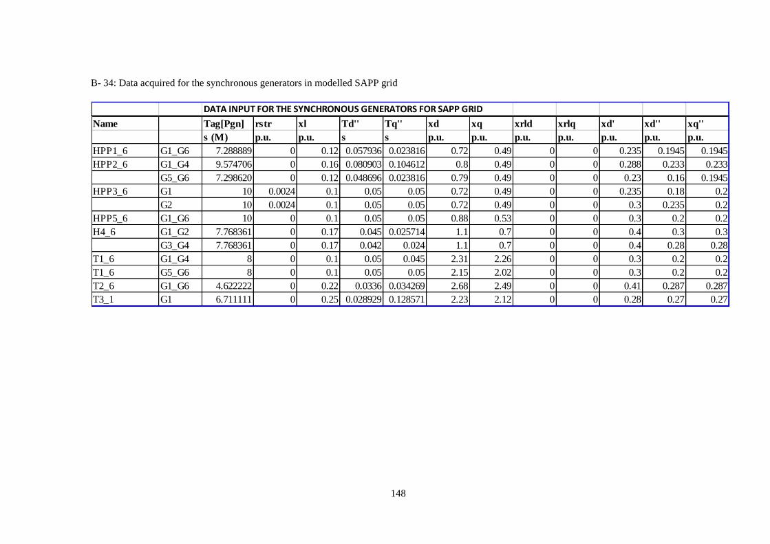
148

B- 34: Data acquired for the synchronous generators in modelled SAPP grid

DATA INPUT FOR THE SYNCHRONOUS GENERATORS FOR SAPP GRID

Name Tag[Pgn] rstr xl Td'' Tq'' xd xq xrld xrlq xd' xd'' xq''

s (M) p.u. p.u. s s p.u. p.u. p.u. p.u. p.u. p.u. p.u.

HPP1_6 G1_G6 7.288889 0 0.12 0.057936 0.023816 0.72 0.49 0 0 0.235 0.1945 0.1945

HPP2_6 G1_G4 9.574706 0 0.16 0.080903 0.104612 0.8 0.49 0 0 0.288 0.233 0.233

G5_G6 7.298620 0 0.12 0.048696 0.023816 0.79 0.49 0 0 0.23 0.16 0.1945

HPP3_6 G1 10 0.0024 0.1 0.05 0.05 0.72 0.49 0 0 0.235 0.18 0.2

G2 10 0.0024 0.1 0.05 0.05 0.72 0.49 0 0 0.3 0.235 0.2

HPP5_6 G1_G6 10 0 0.1 0.05 0.05 0.88 0.53 0 0 0.3 0.2 0.2

H4_6 G1_G2 7.768361 0 0.17 0.045 0.025714 1.1 0.7 0 0 0.4 0.3 0.3

G3_G4 7.768361 0 0.17 0.042 0.024 1.1 0.7 0 0 0.4 0.28 0.28

T1_6 G1_G4 8 0 0.1 0.05 0.045 2.31 2.26 0 0 0.3 0.2 0.2

T1_6 G5_G6 8 0 0.1 0.05 0.05 2.15 2.02 0 0 0.3 0.2 0.2

T2_6 G1_G6 4.622222 0 0.22 0.0336 0.034269 2.68 2.49 0 0 0.41 0.287 0.287

T3_1 G1 6.711111 0 0.25 0.028929 0.128571 2.23 2.12 0 0 0.28 0.27 0.27

149

APPENDIX C TYPES OF POWER TRANSDUCERS CONNECTION IN

POWER SYSTEM

C- 1: Types of transducer connection for power measurement