Embed Size (px)
Citation preview

Noname manuscript No.(will be inserted by the editor)
In-Network Outlier Detection in Wireless Sensor Networks
Joel W. Branch · Chris Giannella · Boleslaw
Szymanski · Ran Wolff · Hillol Kargupta
the date of receipt and acceptance should be inserted later
Abstract To address the problem of unsupervised outlier detection in wireless sensor
networks, we develop an approach that (1) is flexible with respect to the outlier defi-
nition, (2) computes the result in-network to reduce both bandwidth and energy con-
sumption, (3) uses only single-hop communication, thus permitting very simple node
failure detection and message reliability assurance mechanisms (e.g., carrier-sense), and
(4) seamlessly accommodates dynamic updates to data. We examine performance by
simulation, using real sensor data streams. Our results demonstrate that our approach
is accurate and imposes reasonable communication and power consumption demands.
Keywords Outlier detection · Wireless sensor networks
1 Introduction
Outlier detection, an essential step preceding most any data analysis routine, is used
either to suppress or amplify outliers. Suppressing outliers (also known as data cleans-
ing) improves the robustness of data analysis, for instance, in clustering [31], time series
J. W. BranchNetwork Management Research Department, IBM T.J. Watson Research Center, Hawthorne,NY 10532, USA, E-mail: [email protected]
C. GiannellaThe MITRE Corporation, 300 Sentinel Dr Ste 600, Annapolis Junction, MD 20701 USA, E-mail: [email protected]
B. K. SzymanskiNetwork Science and Technology Center and Department of Computer Science, RensselaerPolytechnic Institute, Troy, NY 12180, USA, E-mail: [email protected]
R. WolffDepartment of Information Systems, University of Haifa, Haifa, Israel, E-mail:[email protected]
H. KarguptaDepartment of Computer Science and Electrical Engineering, University of Maryland, Balti-more County, Baltimore, MD 21250, USA, E-mail: [email protected] affiliated with AGNIK, LLC, USA

2
analysis [9] or text categorization [60]. Amplifying outliers helps find rare patterns in
domains such as fraud analysis [47], intrusion detection, and Web purchase analysis.
Several factors make wireless sensor networks (WSNs) especially prone to outliers.
First, they collect their data from the real world using imperfect sensing devices. Sec-
ond, they are battery powered and thus their performance tends to deteriorate as power
dwindles. Third, since these networks may include a large number of sensors, the chance
of error accumulates. Finally, when used for security and military purposes, sensors are
especially prone to manipulation by adversaries. Hence, it is clear that outlier detection
should be an inseparable part of any data processing routine in WSNs.
Simply put, outliers are observations whose probability of occurrence is extremely
small. Since the actual distribution of the data is usually unknown, direct computation
of probabilities is difficult. Because the problem is fundamental, a huge variety of out-
lier detection methods have been developed. In this paper we focus on non-parametric,
unsupervised methods. A simplistic implementation of these methods would require
collecting all data at one central node and executing the outlier detection algorithm
there. Such a centralized solution has several disadvantages in WSNs [34]. The two
most important are (i) the energy overhead incurred by sending the data across the
WSN and (ii) the time delays incurred between data collection and processing. Both
disadvantages increase proportionally to the average distance a data item needs to
travel. They are also exacerbated by the dense flows arising in the areas close to the
central node into which data from the entire WSN, by necessity of a centralized algo-
rithm, converge. The delays increase in such areas because of likely packet collisions,
so either the colliding packets need to be retransmitted, or bandwidth sharing needs to
be imposed. Additionally, the nodes in such areas transmit far more than the average
number of messages, and therefore expend their energy faster than other nodes.
We developed a technique for the computation of outliers in WSNs. This technique
(1) is flexible with respect to the outlier definition, (2) computes the result in-network
to reduce both bandwidth and energy consumption (see, e.g., [30]), (3) uses only single-
hop communication, thus permitting very simple node failure detection and message
reliability assurance mechanisms (e.g., carrier-sense), and (4) seamlessly accommodates
dynamic updates to data. In addition to these essential features, the algorithm pre-
sented here has two highly desirable properties: it is generic – suitable for many outlier
detection heuristics, and its communication load is proportional to the outcome (i.e.,
the number of outliers reported).
We exemplify the benefits of our algorithm by means of two different outlier de-
tection heuristics and 53 sensors, which we simulate using the SENSE network simu-
lator [20] on real data streams. Our results show that the algorithms both converge
to an accurate result with reasonable communication load and power consumption. In
most tested cases, our algorithms outperform the equivalent centralized algorithm.
The rest of the paper is organized as follows. In the next section, we provide a
motivating example, in which a network of acoustic sensors attempts to locate the
possible source of a sound. In Section 3, we discuss related work, including prior publi-
cations on outlier detection, wireless sensor networks, and distributed data mining. We
introduce preliminaries in Section 4 and use them in Section 5 and 6 to describe the
global and semi-global distributed outlier detection algorithms. A the detailed proof of
the correctness of the former is given in the Appendix A. In Section 7 we present the
performance evaluation of our algorithms and our conclusions in Section 8.

3
Fig. 1 The expansion of a sound over time and the possible source location as computed bytwo different pairs of sensors according to the time difference of arrival. The origin of the soundlies in the intersection of the two hyperbolas.
2 Motivating Application
The importance of efficient outlier detection in wireless sensor networks is best under-
stood in the context of popular applications of those systems. Consider, for instance,
the acoustic source localization problem. In this problem, a set of synchronized sensors
all register the arrival of a certain sound at a certain time. Given the distance of two
sensors from one another and the time difference of arrival (TDOA) of the sound, the
possible locations of the source vis-a-vis the two sensors can be deduced. Theoreti-
cally, given data from several sensors, the possible relative locations (each a hyperbola
in the plane) can be intersected and the location of the source pinpointed (see, for
example [3,61] and Fig. 1).
In practice, the problem is much more complex. First, the real terrain in which the
problem occurs is rarely flat, or an unobstructed three-dimensional space. Secondly,
echoes and multiple concurrent sounds may add many possible hyperbolas from which
the relevant ones have to be selected. Last, and perhaps most importantly, the method
is sensitive to errors in sensor synchronization and positioning which may result from
unsuccessful initialization, degradation with time, or power depletion. All these factors
amount to a multiplicity of possible hyperbolas, only a few of which intersect at the
correct location of the source.
A similar principle of localization applies in a broader setting, known as binary
sensing object location [65], in which a single sensor detects an object’s whereabouts
to some accuracy and the neighboring nodes then cooperate to decrease measurement
inaccuracy. Note that the modality of the signal and of the sensor (e.g., acoustic,
seismic, visual, electromagnetic) is irrelevant. Also notice any detection, be it true
or false, of object presence within a sensor’s range will trigger a tracking algorithm or
even the entire tracking service [21]. Such algorithm or service is usually associated with
significant costs, which WSN applications often try to reduce or avoid by using, e.g.,
Maximum Likelihood [59]. Unfortunately, such error reduction methods often require

4
centralization of the raw data which, in itself, can be a costly process; especially when
the sensor outputs a stream of measurements.
It is therefore crucial to be able to perform data cleaning in the network prior to
any decision protocol. With the method suggested in this paper, sensors can constantly
and efficiently prune away data suspected of being false. Only then, and only if the
remaining data seems to require further analysis, would the more complex and costly
procedure for source localization be executed. In this way, much energy can be saved
and system lifetime extended. In the rest of this paper we avoid the discussion of any
specific WSN application, which deserve thorough discussion in their own right (see,
e.g., [12] for source localization and tracking). Instead, we focus on the detection and
elimination of outliers.
3 Related work
3.1 Outlier detection
Outlier detection is a long studied problem in data analysis, and its treatment has
been thoroughly described in several studies [8,33]. An outlier is an observation which
appears to deviate markedly from other members of the sample in which it occurs.
Outlier detection methods can be divided into two kinds: model based, and density
based. Model based methods assume that the data follows a model which, excluding
the specifics of its parameters, is known, so they focus on evaluating the model’s pa-
rameters and singling out the outliers which obstruct their true value. Some methods
assume a statistical model. For instance, the Tietjen-Moore test [64] assumes the data
follows the normal distribution, with unknown mean and variance. However, many
popular methods assume far more abstract models: e.g., that the non-outlier data can
be modeled using a neural network [32,45] or a decision tree [37].
Density based outlier detection methods evaluate the probability of an observation
using the density of data near it. The advantage of this second approach is that no
assumption of a global model for the data source is required but only a metric on
the data domain1. Examples of such metrics include: distance to kth nearest neighbor
[11], [55]; average distance to the k nearest neighbors [6], [11]; inverse of the number of
neighbors within a fixed distance α [42]. A more complicated approach is to utilize both
the local properties of the data (as do the metrics above ) and its global properties, e.g.,
by denoting outliers the n most sparse data points [29]. Alternatively, methods such as
LOF [18] use the ratio of the distance from an observation to its nearest neighbors to
the average of their own distances to their nearest neighbors. The algorithms described
in this work are suitable, as is, to all density based methods except LOF. Generalization
to LOF, while apparently possible, is left for further research.
3.2 Outlier detection in wireless sensor networks
WSNs combine the ability to sense, compute, and coordinate their activities with the
ability to communicate results to the outside world. They have revolutionized data col-
lection in all kinds of environments. Yet, the design and deployment of these networks
1 Often, methods which fall short of even the triangle inequality are sufficient.

5
creates unique research and engineering challenges due to their intended large size (up
to thousands of sensor nodes), their often random and hazardous deployment, obsta-
cles to their communication, their limited power supply, and their high failure rate.
These limitations must be taken into account when developing WSN software. In [28],
Estrin et al. introduce scalable coordination as an important software component. A
survey on the state-of-the-art for WSNs is given in [5], and another survey [4] focuses
on challenges arising from military, health care, ecology, and security applications.
Energy-efficiency is a cardinal WSN requirement and much research has focused
on meeting it [7], [22]. One common strategy for achieving energy-efficiency is by mini-
mizing communication using topology-control algorithms that dictate the active/sleep
cycles of sensor nodes. Examples include ESCORT [16], ASCENT [19], STEM [56],
and GAF [70]. While the focus of this paper is on WSN outlier detection, the chal-
lenge is the same. Hence, while we do not propose a topology-control algorithm, we do
aim to design an energy-efficient algorithm by minimizing the required communication
overhead.
Other research efforts have also focused on developing a framework for distributed
outlier detection in WSNs. Zhuang et al. [72] use a weighted moving average approach
to smooth noise from the data stream arriving at each sensor. Sensors also use data
from neighboring sensors (spatial smoothing) to reduce data propagation to the sink by
not sending observed data whose value remains within the established spatio-temporal
trend. Unlike our approach, theirs does not seek to detect outliers.
Sheng et al. [58] developed a framework for the discovery of k-nearest-neighbor
based outliers: points whose distance to their k-nn exceeds a fixed threshold or the top
n points with respect to the distance to their k-nns. Each sensor maintains a histogram-
type summary of pertinent information over a sliding window of its data points. The
sink node collects these summaries and queries the network for any additional infor-
mation needed to correctly determine the outliers over the whole network. The use
of summaries allows less communication than a naive, centralized approach. Their
approach differs from ours in several ways. First, they only detect outliers over one-
dimensional data and difficulty of of building compact, multi-dimensional histograms
will hinder any extension beyond that. Second, they only consider the two k-nn based
outlier definitions described above, while our approach encompasses these and more.
Thirdly, their approach only applies in settings where spatial proximity is unimportant
while our approach can, if needed, to accommodate spatial proximity (”semi-local”
outlier detection).
Subramaniam et al. [63] require the sensors to maintain a tree communication topol-
ogy and compute outliers using an estimate of the underlying probability distribution
from which the data arises. Such an estimate is computed by each sensor maintaining
a random sample of its data observations. Our approach differs in at least four ways.
First, ours does not make any assumptions about the communication topology (e.g.,
that it is a tree), save that it is connected. Second, ours computes outliers with respect
to all of the data observations at each sensor, not a sample. Third, ours can smoothly
take into account spatial proximity among the sensors (“semi-local” outliers) while
Subramaniam et. al do not focus on this task. Fourth, our approach is designed to
smoothly adjust to changes in the underlying network topology while theirs requires
that the underlying communication tree be reestablished by other means before the
algorithm can resume operation.
Janakiram et al. [36] developed a framework based on a Bayesian Belief Network
(BBN) that has been constructed over the WSN (and distributed to each sensor).

6
Using this, each sensor can estimate the likelihood of an observed tuple and, therefore,
detect outliers, yet it is not clear to what extent the BBN construction phase can be
carried out in-network. Moreover, the authors do not discuss the problem of updating
the BBN given network/data change. In contrast, our processing is entirely in-network
and smoothly adjusts to changes in data/network.
Zhuang and Chen [71] use a wavelet based technique for correcting large isolated
spikes from single sensor data streams. A dynamic time warping (DTW) distance-
based technique is also used to identify more steady intervals of erroneous sensor data
by comparing the data streams of spatially close sensors assumed to produce similar
streams. To reduce energy consumption, anomalous data streams are not transmitted
to the base station. Our method is similar in that it is in-network. However, Zhuang and
Chen’s use of DTW is tightly integrated with a minimum hop count routing algorithm,
which makes the approach more restrictive than ours.
Rajasegarar et al. [54] describe an approach that is based on distributed non-
parametric anomaly detection and requires sensors to maintain a tree communication
network topology. Here each sensor clusters its sampled measurements using a fixed-
width clustering algorithm, then extracts statistics of the clusters (i.e., the centroid
and number of contained data vectors) and then sends them its parent node. The
parent uses its children’s cluster statistics to form a merged cluster. The parent then
transmits that cluster to its own parent. This process continues recursively until the
base station receives all clusters, after which it will perform anomaly detection to
identify all outliers. While this approach supports energy-efficiency by distributing the
clustering operation throughout the network, anomaly detection is only performed at
the base station. Our approach differs in that it distributes the anomaly detection
process itself throughout the network, quickly enabling nodes to identify outliers and
autonomously make further data processing decisions. Nor does our approach rely on
the use and maintenance of a routing tree; hence it smoothly adjusts to changes in the
underlying network topology.
Adam et al. [1] address the issue of accounting for spatially neighboring peers
when detecting outliers in sensor networks. However, they assume the sensor datasets
are centralized and the outlier processing is carried out at the central processing node.
They do not consider the problem of carrying out the outlier detection in-network as
we do.
Palpanas et al. [51] propose a technique for distributed deviation detection using a
network hierarchy of low and high capacity sensors that are differentiated with respect
to processing power and communication range. Here, low capacity sensors aim to detect
local outliers while high capacity sensors detect more spatially dispersed outliers using
an aggregation of low capacity sensors’ data. Kernel density estimators are used to
model the distribution of data values reported by sensors and distance-based detection
techniques are used for identifying outliers. The authors present no formal evaluation
of the proposed technique. Our approach differs in that it does not rely on a hierarchy
of device capabilities.
Radivojac et al. [53] address the process of sensors learning data distributions from
class-imbalanced data. Here, sensors send data points to a central base station which
generates a classification model from class-imbalanced data (i.e., having abundant neg-
ative samples and few positives). the total cost of detection and classification (e.g., costs
of transmitting false positives and false negatives). In contrast, our framework operates
in-network.

7
This paper is an extension of our preliminary work appearing in conference pro-
ceedings [17]. In the extended version we provide complete correctness proofs for the
global outlier detection algorithm along with improved experimental analysis. We have
also added a localized outlier detection algorithm and experimental analysis of it.
3.3 Distributed data mining
Distributed Data Mining (DDM) has recently emerged as an important area of re-
search. DDM is concerned with analysis of data in distributed environments, while pay-
ing careful attention to computation, communication, storage, and human-computer
interaction. Detailed surveys of Distributed Data Mining algorithms and techniques
have been presented in [38], [39], [40]. Some of the common data-analysis tasks include
association rule mining, clustering, classification, kernel density estimation, and so on.
Recently, researchers have started to consider data analysis and data mining in
large-scale dynamic networks with the goal of developing techniques that are highly
asynchronous, scalable, and robust to network changes. Efficient data analysis algo-
rithms often rely on efficient primitives, so researchers have developed several differ-
ent approaches to computing basic operations (e.g., average, sum, max, or random
sampling) on dynamic networks. Mehyar et al. [48] have developed an asynchronous,
deterministic technique for computing an average over a large, dynamic network. Boyd
et al. [15] and Kempe et al. [41] have investigated gossip based randomized algorithms.
Jelasity and Eiben [43] develop the “newscast model.” Bawa et al. [10] have developed
an approach in which similar primitives are evaluated to within an error margin. Wolff
et al. [67] develop a local algorithm for majority voting. Datta and Kargupta [26] have
developed a technique for uniformly sampling data distributed over a large-scale peer-
to-peer network. Bhaduri et al. [13], Sharfman et al. [57], and Wolff et al. [69] have
developed techniques for threshold monitoring over a large, distributed set of data
streams.
Finally, some work has gone into more complex data mining tasks: association rule
mining [67], facility location [44], decision tree induction [14], classification through
meta-learning [46] (all four based on local majority voting), genetic algorithms [23],
k-means clustering [27] [68], Web user community formation [25], hidden variable distri-
bution estimation in a wireless sensor network [49], and outlier detection in distributed
data streams [50] [62].
In the last two papers, Otey et al. [50] and Su et al. [62] address outlier detection
over multiple data streams and wireless sensor networks in particular. Otey et al.
agree with our analysis of two of the main challenges in computing outliers in a sensor
network: The impracticality of collecting all the data to one site and the dynamic nature
of the data. But their work differs from ours in that it ignores the problems associated
with partial message loss and possible sensor failure during the computation. Therefore,
the algorithms they describe use complete passes over all the (distributed) data. Such
passes require that the sensors remain active during every execution of an algorithm
and are sensitive to the dropping of even a few messages. Furthermore, the algorithms
require some form of synchronization between all sensors (in order to move from one
pass to the next) whereas ours only require the minimal level of synchronization –
between the transmitter of a message and its nearby receivers. Achieving global near-
synchronization in a wireless sensor network is not a trivial task. Finally, Otey et al.
focus on their own definition of an outlier, links-based. While this semantic may be

8
suitable for some applications, we choose to focus on implementing more standard
definitions of an outlier.
Su et al. take a very different approach. They employ a more standard definition
of an outlier, kernel based density estimation, which is an approximation for distance
based density. Their work differs from ours and that of Otey at el. mainly in its as-
sumption of a hierarchical sensor network architecture in which leaders collect data
from their subject nodes. While a hierarchical architecture greatly simplifies many al-
gorithms, it is often unsuitable for real deployments of wireless sensor networks. The
leaders, almost by definition, require many more resources than their subjects and
therefore quickly deplete their power or suffer from communication congestion. When
that happens, new leaders have to be selected; much system time is thus invested in
maintaining the computational architecture. Therefore, the work of Su et al. might
be better than ours for hybrid scenarios in which some sensors (e.g., those with fixed
power connections) are naturally the leaders. Our work, in comparison, might be more
suitable for the classic scenario in which identical sensors are randomly deployed and
must self-organize to form a network.
4 Preliminaries
4.1 Outlier detection defined
Let D be a data space. Following a common approach, our outlier detection method
relies on a ranking function, R. This function maps x ∈ D and finite D ⊆ D to a
non-negative real number R(x,D), indicating the degree to which x can be regarded
as an outlier with respect to a dataset D. Some common examples of R include the
density metrics mentioned in the previous section. We assume that a fixed total linear
order, ≺, on D is used as a tie-breaking mechanism to ensure that R(., Q) creates a
total linear ordering on D for any finite Q ⊆ D.
R is assumed to satisfy the following two axioms. Given x ∈ D, for all finite
Q1 ⊆ Q2 ⊆ D: anti-monotonicity, R(x,Q1) ≥ R(x,Q2); smoothness, if R(x,Q1) >
R(x,Q2), then there exists z ∈ Q2\Q1, such that R(x,Q1) > R(x,Q1∪{z}). The anti-
monotonicity axiom is similar to the a-priori rule in frequent itemset mining [2]. The
smoothness axiom expresses the intuition that R changes gradually. As more points
are added to Q1, the rating function changes gradually to R(x,Q2). Of the examples
in the previous paragraph, all but LOF satisfy these assumptions, assuming, as we do,
the use of a tie-breaking mechanism as described in the previous paragraph.
Given n, a user-defined parameter, and a finite dataset D ⊆ D, the outliers of D
are denoted On(D) and are defined to be the top n points in D with respect to R(., D)
(if |D| < n, then On(D) is defined to be D).
4.2 Distributed system set-up
The distributed system architecture we assume consists of a collection of sensors, pi,
each producing a finite dataset Di ⊆ D. Di only contains points that originated at
sensor pi, for example, a data point associated with a measurement made by pi. Sensors
communicate by exchanging messages with their immediate neighbors as defined by
an undirected graph. We assume that messages are reliable, i.e., the sender will be

9
informed if a message is not received, and each sensor pi can accurately maintain the
list of its immediate neighbors, Γi, in the graph. Our algorithms work as long as there
exists a path, possibly unknown, from each sensor to every other sensor. Note that
message reliability is difficult to fully maintain in a WSN – some message dropping is
expected. While our algorithm assumes no message dropping, the WSN simulator we
used in our experiments realistically includes message dropping. We used an end-to-
end acknowledgement mechanism to largely mitigate the effect of message dropping.
A small number of messages are still lost, but the algorithm achieves 99% accuracy.
4.3 Notation Summary
Table 1 is provided as an aid to understanding the notation we use throughout the
paper. A summarized definition is provided with each symbol listed, as well as, the
subsection where a complete definition can be found. Note that some of the symbols
listed in the table, e.g., Dii,j , are only fully defined later in this paper.
D Space from which all data points are drawn.R(., .) Outlier ranking function for a data point (first Section 4.1.
argument) with respect to a set of points (second).On(.) Top n outliers in a set of data points
with respect to R(., .).
pi The ith sensor.Γi The immediate neighbors of pi in the Section 4.2.
communication graph.Di The data points produced by pi.D All data points in the network.Di
i,j The data points pi is holding that
pi sent to pj .Di
j,i The data points pi is holding that Section 5
pj sent to pi. before 5.1.P i All the data points pi is holding.N(., .) The nearest neighbor of a data point (first Section 5.1.
argument) among a set of points (second).[.|.] The support set of a data point or set of Section 5.2.
points (second argument) with respect to anotherset of points (first).
⋃
j Dj [hops to i ≤ d] The union of all Dj
where the hop distance between pj and pi ≤ d.x.hop An addition field on data point x to account
for hop distance.x.rest The remaining fields on data point x. Section 6
before 6.1.Q≤h The subset of data points in Q with
hop field ≤ h.[Q]min The result of replacing all points in Q
that differ only in their hop field bythe point with the smallest hop field.
Table 1 Notation table: symbol, summarized definition, and section where complete definitionappears.

10
5 Global distributed outlier detection algorithm
In this section, we describe a distributed algorithm by which sensors, each assumed
to know R and n, compute On(D) where D =⋃
i Di (global outlier detection). In a
wireless sensor network, it can be desirable for sensors to find outliers only with respect
to the data contained in nearby sensors, rather than in the entire network (semi-global
outlier detection). In section 6, we describe how to modify the global outlier detection
algorithm to act in a semi-global manner.
At any point in time, pi keeps track of the data points it has sent to or received
from its neighbor pj at some past time. Let Dii,j denote the set of points sent from pi
to pj , and, Dij,i denote the set of points sent from pj to pi. Importantly, (Di
i,j ∪ Dij,i)
denotes the data points that pi can be sure are commonly held with pj (there may
be more). Let Pi denote Di
⋃
j∈ΓiDi
j,i, the set of points pi is holding at the current
time.2 pi uses Pi to compute an estimate of the overall correct answer, On(D). The
estimate of pi is On(Pi), the set of outliers based on all the information available to pi
at the current time.
The algorithm does not assume any special sensors. Each sensor, pi, asynchronously
waits for an event to occur: (i) the algorithm is initialized, (ii) Di changes, (iii) a
message is received from a neighbor, or (iv) a link goes up/down, causing the immediate
neighborhood of pi to change (however, algorithm correctness requires that we assume
the network remain connected). Note that events for pi are entirely local and can be
detected without the aid of any other sensors beyond the immediate neighborhood.
Once pi detects an event, it will decide which of the points it is currently holding (Pi),
if sent, could cause its neighbor, pj , to change its estimate. pi then sends these points
and adds them to Dii,j (pi carries out this process separately for all of its neighbors).
Gradually, the set of points held by each sensor becomes large enough to obtain
overlap so that each sensor’s estimate is the correct answer, On(D). This will be guar-
anteed to occur once each sensor, individually, decides that none of the points it is
currently holding need be sent to its neighbors. At this point, the algorithm is termi-
nated. To see how all of this works, consider an example.
5.1 Example
Let R be the distance to the nearest neighbor and, given x ∈ D and finite P ⊆ D,
let N(x, P ) denote the nearest neighbor of x among points in P . Given finite Q ⊆ D,
let N(Q, P ) denote⋃
x∈Q N(x, P ). Let n = 1 and consider a network of two sensors,
pi and pj , each initially holding the following one-dimensional datasets. The correct
answer the algorithm will compute is On(D) = {0.5}.
– Di = {0.5, 3, 6, 10, 11, . . . , a}.
– Dj = {4, 5, 7, 8, 9, a + 1, a + 2, . . . , a + b}.– D = Di ∪ Dj = {0.5, 3, 4, 5, 6, 7, 8, 9, 10, 11, . . . , a, a + 1, . . . , a + b}.
Initially, Pi = Di, Pj = Dj , and Dii,j = Di
j,i = Dji,j = D
jj,i = ∅. For simplicity, we will
describe the algorithm in synchronous fashion starting with pi. But the ideas extend
nicely to asynchronous operation.
2 Note the distinction between Di and Pi. Di is the set of points that originated at sensorpi, while Pi is the set of all points that pi is holding including Di and those originating atother sensors but propagated to sensor pi through message passing.

11
1. pi computes its estimate as On(Pi) = {6} and then must compute the set of its
data points that might cause pj to change its estimate if sent. We call these the
sufficient points from Pi for sensor pj . Formally, we define a set Zj ⊆ Pi to be
sufficient for pj if
[On(Pi) ∪ N(On(Pi), Pi)] ∪[
N(On(Dii,j ∪ D
ij,i ∪ Zj), Pi)
]
⊆ Zj . (1)
The rationale for the first part is simple. On(Pi) is necessary for pj , because if pi is
right in its estimate, then pj ought to know about it. Moreover, pi must also send
N(On(Pi), Pi), because this allows pj to determine if any of its points can cause
the ranking of the points in On(Pi) to change.
The rationale for the second part is somewhat more complex. In brief, if pi were
to send Z ⊆ Pi to pj , then pi would also need to send N(On(Dii,j ∪ Di
j,i ∪Z), Pi).
To avoid re-sending, pi requires that N(On(Dii,j ∪ Di
j,i ∪ Z), Pi) be contained in
Z. To understand the reasoning for all of this, consider that (Dii,j ∪ Di
j,i ∪ Z) is
the total set of points pi knows pj would have if Z had been sent to pj . Thus,
On(Dii,j ∪ Di
j,i ∪Z) is the best approximation pi would have to the estimate of pj
if Z were sent to pj . Hence, pi computes its nearest neighbors to these, because, if
pi is right in its approximation, it must ensure that pj have these neighbors since
they could cause pj to change its estimate.
Getting back to our example, observe that On(Pi) ∪ N(On(Pi), Pi) = {3, 6}. More-
over, N(On(Dii,j ∪ Di
j,i ∪ {3, 6}), Pi) = N(On({3, 6}), Pi) = {3} ⊆ {3, 6}. Hence,
Zj = {3, 6}, as this satisfies (1) above. So, pi sends {3, 6} \ (Dii,j ∪ Di
j,i) = {3, 6}
and updates Dii,j to {3, 6}.
2. pj will receive these points and update Dji,j to {3, 6} (currently D
jj,i = ∅). It is thus
implicit that Pj now denotes Dj ∪Dji,j = {3, 4, 5, 6, 7, 8, 9, a+1, a+2, . . . , a+b}. pj
computes On(Pj) ∪ N(On(Pj), Pj) = {3, 4} (assuming appropriate tie-breaking).
Moreover, it can be seen that this satisfies (1). So, pj sends {3, 4} \ (Dji,j ∪ D
jj,i)
= {3, 4} \ {3, 6} = {4} and updates Djj,i to {4}.
3. pi receives these points and updates Dij,i to {4} (currently Di
i,j = {3, 6}). It is thus
implicit that Pi now denotes Di ∪ Dij,i = {0.5, 3, 4, 6, 10, 11, . . . , a}. pi computes
On(Pi) ∪ N(On(Pi), Pi) = {0.5, 3}. Moreover, it can be seen that this satisfies (1).
So, pi sends {0.5, 3} \ (Dii,j ∪Di
j,i) = {0.5, 3} \ {3, 4, 6} = {0.5} and updates Dii,j
to {0.5, 3, 6}.4. pj will receive these points and update D
ji,j to {0.5, 3, 6} (currently D
jj,i = {4}).
It is now implicit that Pj now denotes Dj ∪ Djj,i = {0.5, 3, 4, 5, 6, 7, 8, 9, a + 1, a +
2, . . . , a + b}. pj computes On(Pj) ∪ N(On(Pj), Pj) = {0.5, 3}. Moreover, it can
be seen that this satisfies (1). So, pj sends {0.5, 3} \ (Dji,j ∪ D
jj,i) = {0.5, 3} \
{0.5, 3, 4, 6} = ∅. In other words, nothing is sent.
At this point the algorithm has terminated, both sensors are waiting for an event to
occur, and there are no messages in flight. Pi and Pj denote {0.5, 3, 4, 6, 10, 11, . . . , a}and {0.5, 3, 4, 5, 6, 7, 8, 9, a + 1, a + 2, . . . , a + b}, respectively. Therefore On(Pi) =
{0.5} = On(Pj), which in turn, equals the correct answer On(D). Observe that the
total amount of communication (data points sent) was 4. The naive approach, which
centralized all the data on either pi or pj , requires min{a−6, b+5} communication.
For large min{a, b}, the distributed algorithm requires much less communication.

12
5.2 The algorithm
To translate the previous example into a formal algorithm for general R (satisfying the
anti-monotonicity and smoothness axioms), we must provide some definitions general-
izing the role of N(., .). Given x ∈ D and finite P ⊆ D, Q1 ⊆ P is called a support set
of x ∈ D over P if R(x, P ) = R(x,Q1). Intuitively, we can see that all other points
from P can be discarded without affecting the rank of x. Using cardinality and the
tie-breaking mechanism discussed earlier (≺ a total linear order on D), we can define a
unique, smallest support set of x with respect to P , denoted [P |x].3 Given Q ⊆ P , let
[P |Q] denote⋃
x∈Q[P |x]. In the previous example, R was the distance to the nearest
neighbor, so, [P |x] equaled N(x, P ) using ≺ to break ties.
With these more general definitions, we define a set Zj ⊆ Pi to be sufficient for pj
if
(On(Pi) ∪ [Pi|On(Pi)]) ∪(
[Pi|On(Dii,j ∪ D
ij,i ∪ Zj)]
)
⊆ Zj . (2)
Due to the broadcast nature of wireless sensor network communication, pi cannot send
points to one immediate neighbor without the other neighbors receiving them as well.
In light of this, the algorithm accumulates all points (tagged with recipient IDs) to be
sent to all immediate neighbors in a single packet, M . When an immediate neighbor,
pj , receives M , the neighbor extracts those points that are tagged with ID j. If no
points are tagged as such, pj does not regard receipt of M as an event.
pi detects an event if one of the following occurs: (i) the algorithm is initialized,
(ii) Di changes, (iii) M is received and contains points tagged with i (i.e., points
are received from a neighbor), or (iv) a link goes up/down, causing pi’s immediate
neighborhood to change (however, algorithm correctness requires that we assume the
network remain connected). In response, pi carries out the following algorithm whose
pseudo-code is given in the “Global Outlier Detection” Figure. First, Pi is updated to
account for all pj from which points were received in M . Only points not already in
Pi are added to Dij,i. The first two steps in the main for-loop (“For each j ∈ Γi, do”)
compute a Zj satisfying Equation (2), although the result is not guaranteed to be the
smallest set to do so. The “If....then” in the main for-loop tests whether there are any
points found sufficient for pj that pi cannot already be sure pj has, i.e., points in Zj
but not in Dij,i ∪ Di
i,j . If any such points are found, they are added to M along with
their recipient ID j.
5.3 Streaming data and peer addition/deletion
We now extend the algorithm to one supporting a sliding window over a stream of
data sampled at each sensor. To support this, we assume each point is time-stamped
when it is sampled. We further assume that sensor clocks are synchronized to the extent
required by the application for whom outlier detection is a preceding step. Thus, sensor
pi can delete all points in Pi (regardless of where they were originally sampled) once
their time-stamp indicates they have expired.
The algorithm still needs to be modified to accommodate the addition of sensors
during operation. All that is required is to treat the arrival of a new sensor as an event
3 Formally, given Q1, Q2 ⊆ P support sets of x with respect to P , Q1 is smaller than Q2 if|Q1| < |Q2| or (|Q1| = |Q2| and Q1 is lexicographically smaller than Q2 with respect to ≺).

13
Fig. 2 Global Outlier DetectionAlgorithm 1
– Set M = ∅, and, update Pi accounting for all neighbors pj from which points werereceived. For each point x received from pj , do the following. If x is not already Pi, thenadd x to Di
i,j .
– For each j ∈ Γi, do– – Set Zj = On(Pi) ∪ [Pi|On(Pi)].– – Repeat until no change: Zj = Zj ∪ [Pi|On(Di
i,j ∪ Dij,i ∪ Zj)].
– – If Zj \ (Dii,j ∪ Di
j,i) is non-empty, then
– – – Append 〈j, Zj \ (Dii,j ∪ Di
j,i)〉 to M .
– – – Add points in Zj \ (Dii,j ∪ Di
j,i) to Dii,j .
– – End If.– End For.– If M is non-empty, broadcast it to all sensors in Γi.
end
for the new sensor and for all its immediate neighbors. The algorithm can also be
modified to accommodate the removal of sensors (e.g., when their battery is depleted),
assuming that the network remains connected. In the sliding window model, a simple
strategy is to merely allow points that originated with the removed sensor to age out
of the window. The consequence of that would be that the result would not be the
same as would be computed from the data of all active sensors. This usually poses no
practical problem. A more general and complex solution is to propagate messages into
the network, causing sensors to explicitly delete those points that originated with the
removed sensor. We leave the details of this approach to future work.
5.4 Algorithm correctness
The correctness of the algorithm can be proved in the following sense: if the data and
network links remain static (and the network is connected), then communication will
eventually stop, at which point all the sensors’ outlier estimates will equal On(D). This
does not mean that the algorithm cannot handle dynamic changes or network links; it
merely means that the algorithm will respond to such changes or links by converging
to the correct answer. Since convergence takes time, and since during that time further
changes are possible convergence to a globally correct value is only assured on the
condition that the data and network remain unchanged long enough.
It is easy to see that, barring changes in the data or network, the algorithm will
always terminate. So, the proof proceeds in two steps. First, upon termination, all sen-
sors have the same outlier estimates and support (Theorem 1). Second, the consistent
estimates shared by all sensors are indeed the correct ones (Theorem 2). Proofs of
Theorems 1 and 2 are provided in Appendix A.
Theorem 1 Assuming a connected network, if for all sensors pi, Di and Γi do not
change, then upon termination of the algorithm, all sensors’ outlier estimates and sup-
ports agree. I.e., for all pi, pj , On(Pi) = On(Pj) and [Pi|On(Pi)] = [Pj |On(Pj)].
Theorem 2 Assuming a connected network, if for all sensors pi, Di and Γi do not
change, then upon termination of the algorithm, all sensors’ outlier estimate will be
correct. I.e., for all pi, On(Pi) = On(D).

14
Comments: 1) Theorem 1 holds without the smoothness axiom; hence, for any anti-
monotonic R, upon convergence, all sensors will agree on their outlier estimate and
support. However, without the smoothness axiom, Theorem 2 does not hold, i.e., the
consistent outlier estimates might not be the correct ones. Counter-examples exist
showing how an anti-monotonic but not smooth R causes the algorithm to terminate
without all sensors agreeing upon the correct set of outliers.
2) For an arbitrary R, it is not clear how to efficiently compute [P |x] and we do
not address the issue. However, efficient computation is straightforward for the R we
consider in our experiments: average distance to the kth nearest neighbor.
3) The correctness proof requires reliable communication, e.g., no message drop-
ping. The WSN simulator we used in our experiments includes message dropping. We
used an end-to-end acknowledgement mechanism to largely mitigate the effect of mes-
sage dropping, and the algorithm achieved 99% accuracy.
6 Semi-Global Distributed Outlier Detection Algorithm
For many applications, computation only takes into account samples which were taken
close to one another. In such applications outliers should also be computed respective
to the data sampled by nearby sensors, rather than by the entire network. In this
section, we describe how to modify the global outlier detection algorithm to act in
a semi-global manner. Under this approach, each sensor computes outliers only from
within those points sampled in its spatial proximity.
To account for spatial locality, we use hop distance: the number of hops between
two sensors along their shortest path in the underlying communication network. Given
integer d and sensor pi, let⋃
j Dj [hops to i ≤ d] denote the union of all Dj such that pj
and pi have hop distance no greater than d. The semi-global outlier detection problem
requires each pi to compute On(⋃
j Dj [hops to i ≤ d]). Setting d to infinity yields the
global outlier detection problem discussed earlier.
To account for hop distance, each data point x has an additional field x.hop (at
birth x.hop is set to zero). Let x.rest denote all the remaining fields – these are the
ones used by the rating function R. Given a set of points Q, for 0 ≤ h ≤ d, let Q≤h
be the set of points x ∈ Q with x.hop ≤ h. Let [Q]min be the result of replacing all
points that differ only in their hop field by the point with the smallest hop field. For
example, consider Q = {w, v, x, y, z} where w.rest = v.rest, x.rest = y.rest = z.rest,
and v.rest 6= x.rest. If w.hop < v.hop and x.hop < y.hop, z.hop, then [Q]min = {w, x}.
6.1 Semi-global outlier detection algorithm
The basic idea of the semi-global outlier detection algorithm is that each sensor pi
will run the global outlier detection algorithm over only those points arising on sensors
within d hops. At first glance, the following simple modification of the global algorithm
seems adequate. Before pi sends a copy of a point, x, to its neighbors, it first increments
x.hop and sends only if x.hop ≤ d. Unfortunately, such a simple modification will
not work. It does not take into account the fact that x must not have any effect on
the outlier determination process of sensors pj whose distance from pi is more than
d − x.hop. Examples can be demonstrated wherein this omission causes an incorrect
overall result.

15
Fig. 3 Semi-Global Outlier DetectionAlgorithm 2
– Set M = ∅, and, update Pi accounting for all neighbors pj from which points werereceived. For each point x received from pj , do the following. If there does not exist y inPi with x.rest = y.rest, then add x to Pi (and update Di
i,j), otherwise if x.hop < y.hop,
then replace y with x in Pi (updating as needed Di and Dif,i
for each f ∈ Γi).
– For each j ∈ Γi, do– – For h = 0 to d − 1– – – Set Zh
j = On(P≤hi ) ∪ [P≤h
i |On(P≤hi )].
– – – Repeat until no change: Zhj = Zh
j ∪ [P≤hi |On(Di,≤h
i,j ∪ Di,≤hj,i ∪ Zh
j )].
– – – Increment the hop field for each point in Zhj .
– – End For.
– – Set Zj =[
⋃d−1
h=0Zh
j
]min.
– – Remove points x from Zj such that there exists y ∈ (Dii,j ∪Di
j,i) with x.rest = y.rest
and y.hop ≤ x.hop.– – If Zj is non-empty, then– – – Append 〈j, Zj〉 to M .– – – Update Di
i,j by adding the points in Zj .
– – End If.– End For.– If M is non-empty, broadcast it to all sensors in Γi.
end
To avoid this problem, pi must partition Pi into d parts: P≤hi for 0 ≤ h ≤ d − 1.
For each of these parts, the global outlier detection algorithm is applied independently.
Upon detecting an event (defined as before), pi executes the algorithm whose pseudo-
code is given in Figure 2.
First, Pi is updated to account for all pj from which points were received in M .
Because of the hop fields, the update step is somewhat more complicated than that
of the global outlier detection algorithm. A point x from pj is added to Dij,i if there
does not exist y ∈ Pi with x.rest = y.rest (x does not already appear in Pi). Or, if
there does exist y ∈ Pi with x.rest = y.rest, but x.hop < y.hop, then x replaces y in
Pi (updating as needed Di and Dif,i for each f ∈ Γi). Note that there cannot be more
than one y with the same rest fields as x since all but the point with the smallest hop
would have been removed earlier.
Next, for each neighbor pj and each 0 ≤ h ≤ d − 1, a set Zhj is computed which
satisfies (2) with Zj , Pi, Dii,j , and Di
j,i replaced by Zhj , P
≤hi , D
i,≤hi,j , and D
i,≤hj,i ,
respectively. This computation is done by the first steps inside the nested for loops.
Then, the hop field for each point in Zhj is incremented in preparation for sending to
pj .
Once all 0 ≤ h ≤ d − 1 have been processed for pj (the inner for loop completes),
Z1
j · · ·Zd−1
j are unioned and redundancies are eliminated. For any pair of points x, y
in⋃d−1
h=0Zh
j , if x.rest = y.rest and x.hop < y.hop, then y is dropped (this action
is signified by the ‘min’ superscript in the step immediately after the inner for loop).
Then, all points x are removed from Zj if there exists a point y in (Dii,j ∪Di
j,i) with the
same rest fields but y.hop ≤ x.hop. If the resulting Zj is non-empty, then these points
are added to M (along with ID j) for broadcast to neighbors, and Dii,j is updated by
adding the points in Zj .

16
7 Performance Evaluation
7.1 Experimental setup
We used the SENSE wireless sensor network simulator [20] to evaluate the performance
of the global and semi-global outlier detection algorithms. Specifically, we analyzed
the following metrics: (1) the accuracy of the algorithms in detecting outliers; (2) the
average energy consumption per node per sampling period, as well as its breakdown
to transmission related, and reception related consumption; and (3) the minimum and
maximum energy consumption in the network. We observed both the global and semi-
global outlier detection algorithms to be highly accurate; nodes converged upon the
correct results approximately 99% of the time. We attribute any detection error to
dropped packets (despite the ”end-to-end” acknowledgement mechanism being used).
Since average detection accuracy was consistent across all simulation parameters, we
did not include any accuracy-related plots.
Various scenarios were used to analyze the performance of our algorithms. First,
we compared our algorithms’ energy consumption to that of a purely centralized out-
lier detection algorithm. Here, all nodes periodically sent their sliding window contents
to a central node, which detected outliers using the unioned data sets and returned
the outliers back to the nodes. For simplicity, we configured the centralized algorithm
to calculate only global outliers because for this algorithm, energy consumption is in-
dependent of whether global or semi-global outliers are detected. Also, all algorithms
(including the centralized solution) were evaluated using the following two outlier rank-
ing functions (R, in our terminology): distance to nearest neighbor (NN) and average
distance to k nearest neighbors (KNN).
We chose a centralized algorithm for our comparison because, to the best of our
knowledge, there exist no comparable distributed solutions for WSN outlier detection.
We find such a comparison to still be valid as many WSN deployments continue to
employ centralized configurations, citing ease of administration as well as maintenance
of a single (and ”standard”) point of interface with the growing number of applications
and systems in the sense-and-respond computing domain. Such reasons, however, do
not preclude the utility of a distributed algorithm such as ours, since it remains very
useful as a general data processing solution for a wide range of applications, centralized
are not.
For our data sets, we used real-world recorded sensor data streams from [35], in
which distributed data samples are both spatially and temporally correlated. The data
set is composed of a series of data samples describing environmental phenomena such as
heat, light, and temperature from 53 sensors which periodically transmitted individual
data samples to a central base station. The data set has some missing data points, which
to the best of our knowledge is largely due to packet loss. Following accepted practices,
we replaced missing data points with the average values of the data points within the
sliding windows that preceded the missing points. This helped retain the temporal
trends of the data streams. The data points contained the following features: (1) ID of
the sensor that produced the data point; (2) epoch (sequential number denoting the
data point’s position in the sensor’s entire stream); (3) data value (we specifically used
temperature); and (4) x,y location coordinates. We used the data points’ temperature
value and location coordinates as inputs into the outlier rating functions. The location
coordinates can represent the place where the measurements were taken or an estimate
of a target’s position or some other spatial information. It is important to note that

17
Fig. 4 53 node network topology (from [35]) used in all simulations reported.
these coordinates are attributes of the data on which our algorithm works in the exam-
ple. They might become erroneous or anomalous just like any other data attribute, due
to inaccurate initialization, power degradation, or a transmission error. The algorithm
itself, however, would work the same regardless of whether such coordinates are given.
We originally simulated two networks, one containing all of the 53 nodes, with each
node placed according to the coordinates in the data (thus matching the real topology
from [35]), and the other containing 32 randomly selected nodes. By comparing the two
networks we intended to study the scale-up properties of the algorithms. However, since
the simulations revealed no real performance difference between the two networks, we
eventually chose to only include results from the simulation of the full, 53 node network.
The topology of the network is shown in Figure 4.
The terrain dimensions in our network simulation are 50m×50m. Most hardware
specifications claim that a sensor node’s transmission range typically reaches up to ap-
proximately 250m, when properly elevated. However, when placed on the ground the
reported ranges are much smaller [73] and, for reliable indoor communication using
Crossbow motes, the effective range drops to a few meters [66]. Therefore, we con-
figured all nodes to have a uniform transmission range of approximately 6.77m. We
also used the hardware energy model based on the Crossbow mote specifications [24],
with a transmit/receive/idle power setting of 0.0159W/0.021W/3e-6W (assuming a 3V
power source). We simulated the wireless transport medium using the free-space signal
propagation model.
Two protocols were used for routing. For the distributed algorithms, we used simple
broadcast (as opposed to unicast) transmission with promiscuous listening that allowed
all nodes to send data points to all their adjacent neighbors using one transmission.
For the centralized algorithm, we used the well-accepted AODV [52] wireless routing
protocol for multi-hop communication. We note that a simple end-to-end acknowledg-
ment mechanism was also used to reinforce reliable communication. While alternative
protocols do exist for more data-centric and energy-efficient communication, our main
goal was straightforward comparison of the algorithms without having to balance the
various advantages of each.

18
All simulations were run for 1000 seconds of simulated time and were repeated up
to 12 times using different random number generator seed values to obtain averaged
results (most results are based on 12 simulation runs, some were based on 6). Error bars
are included with each point in each plot showing 95%, Student’s T, confidence intervals
(some bars are very small and appear not to be present). As shown in the following plots
(and the tables in Appendix B), we collected results for different values of the following
algorithm parameters: (1) the length of the node’s sliding window, w ; and (2) the
number of outliers to be reported, n. Additionally, for the distributed localized outlier
detection algorithm, the hop diameter was varied from one to three. Plot data are
labeled as follows: (1) Centralized for results obtained with the centralized algorithm;
(2) Global−NN and Global−KNN for results obtained using distributed global outlier
detection with NN and KNN outlier detection ranking functions (R), respectively; and
(3) Semi−global, epsilon = x for all results obtained using distributed localized outlier
detection with hop diameter x. For brevity, we will often refer to the different algorithms
by these labels.
7.2 Experimental results
The numbers (averages, confidence intervals) from all of the following plots are dis-
played in tables in Appendix B.
7.2.1 Effect of sliding window size
Figure 5 compares network energy consumption per sampling interval with increasing
w but n and k fixed at 4. Here, we show separate plots for transmission (TX) and
reception (RX) energy for the reader who is interested in the disparity between the
energy consumption due to different radio operations. We note that data points are
missing for Global-KNN at w=40, due to a computational limitation of our simulator.
However, preliminary results based on similar simulations and statistics are shown
in [17]. Since the trends between both sets of results are nearly identical for the non-
missing data points, it is reasonable to extrapolate the values of the missing points
here.
Both figures show that as w increases, Global-NN is the only algorithm that reduces
its energy consumption. Figure 5 shows that Global-NN eventually becomes the most
energy-efficient solution given the domain of w. We attribute Global-NN’s reduction
in energy consumption to an increase in incoming data redundancy as the size of the
sliding window increases. Since Global-NN only uses one supporting point to determine
an outlier, the probability of finding new outliers or supports with this scheme in each
new time interval as the sliding window increases is low.
Global-KNN and Centralized consume, as can be seen in Figure 5, more energy as
w increases. However, given comparable results in [17], we can extrapolate that Global-
KNN’s energy consumption is a concave increasing function of w, whereas Centralized’s
is a convex increasing function, which makes the latter comparatively less energy-
efficient in that it approaches a point of network failure at a higher rate. By contrast,
the energy trend for Global-KNN for this data set indicates that when global outliers
are defined by multiple supporting points (in this case 4), the increasing time interval
from which the points are chosen has a less drastic effect on the number of messages
required for the algorithm to converge. Overall, in cases where a user prefers to use a

19
0.0001
0.001
0.01
0.1
5 10 15 20 25 30 35 40 45
Avg
. TX
ene
rgy
per
node
per
sam
ple
inte
rval
(J)
Sliding window size
CentralizedGlobal-NN
Global-KNN
0.0001
0.001
0.01
0.1
5 10 15 20 25 30 35 40 45
Avg
. RX
ene
rgy
per
node
per
sam
ple
inte
rval
(J)
Sliding window size
CentralizedGlobal-NN
Global-KNN
Fig. 5 Average transmission and reception energy consumption per node per sample intervalvs. w (n=4, k=4) for global outlier detection.
higher number of supporting points and a larger sliding window to define outliers, the
energy consumption of Global-KNN will be higher, but it is still more energy efficient
than Centralized.
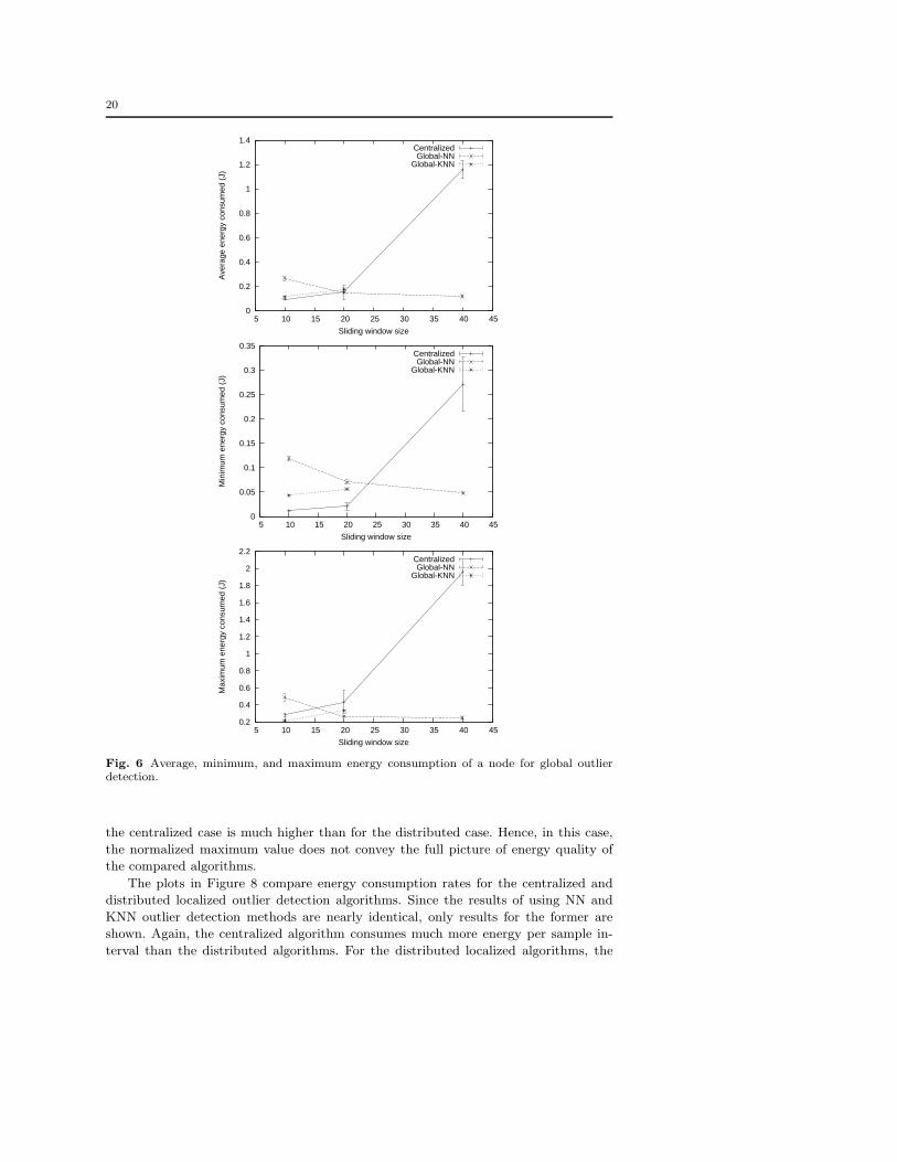
Balanced energy consumption is important for the longevity of a sensor network
as an operating system. Figure 6 compares the minimum, average, and maximum
energy consumption for a sensor node as w increases. This view further accentuates
the advantage of using the Global-NN outlier detection solution over Centralized for
large window sizes. In Centralized, some motes consume by far more energy than others.
This would lead, in a real application to the quick depletion of their energy. Since those
motes usually consume that much energy because they are critical to the algorithm, this
would endanger the livelihood of the system. Another observation is that the range of
energy consumption for different motes running the same detection algorithm is larger
for the centralized solution than for the distributed solution. Figure 7 illustrates this
clearly by showing the values from Figure 6, normalized with respect to the average
energy consumption. For w=10, the most energy consuming node consumed nearly
three times more energy than the average node in a centralized algorithm and less
than twice the energy of the average node in both distributed algorithms.
For the partial information for w=40, the normalized range of energy consumption
is actually lower for the centralized algorithm than for the distributed one. However,
referring back to Figure 6, we see that the average energy consumption for a node in
20
0
0.2
0.4
0.6
0.8
1
1.2
1.4
5 10 15 20 25 30 35 40 45
Ave
rage
ene
rgy
cons
umed
(J)
Sliding window size
CentralizedGlobal-NN
Global-KNN
0
0.05
0.1
0.15
0.2
0.25
0.3
0.35
5 10 15 20 25 30 35 40 45
Min
imum
ene
rgy
cons
umed
(J)
Sliding window size
CentralizedGlobal-NN
Global-KNN
0.2
0.4
0.6
0.8
1
1.2
1.4
1.6
1.8
2
2.2
5 10 15 20 25 30 35 40 45
Max
imum
ene
rgy
cons
umed
(J)
Sliding window size
CentralizedGlobal-NN
Global-KNN
Fig. 6 Average, minimum, and maximum energy consumption of a node for global outlierdetection.
the centralized case is much higher than for the distributed case. Hence, in this case,
the normalized maximum value does not convey the full picture of energy quality of
the compared algorithms.
The plots in Figure 8 compare energy consumption rates for the centralized and
distributed localized outlier detection algorithms. Since the results of using NN and
KNN outlier detection methods are nearly identical, only results for the former are
shown. Again, the centralized algorithm consumes much more energy per sample in-
terval than the distributed algorithms. For the distributed localized algorithms, the

21
Fig. 7 Normalized average, minimum, and maximum amount of energy consumed by a nodefor global outlier detection.
rate of energy consumption increases along with the values of epsilon (the hop range).
This is expected because, as epsilon increases, so does the message passing overhead
as data points travel farther from their place of origin. The behavior of the distributed
algorithm in the localized case for nearest neighbor outlier detection is similar to that
of global case for the same detection method. Energy consumption generally decreases
as w increases. As before, we attribute this behavior to the increased data redundancy
as the size of the sliding window increases. In general, the extent of the spatial area

22
1e-005
0.0001
0.001
0.01
0.1
5 10 15 20 25 30 35 40 45
Avg
. TX
ene
rgy
per
node
per
sam
ple
inte
rval
(J)
Sliding window size
CentralizedSemi-global, epsilon=1Semi-global, epsilon=2
1e-005
0.0001
0.001
0.01
0.1
5 10 15 20 25 30 35 40 45
Avg
. RX
ene
rgy
per
node
per
sam
ple
inte
rval
(J)
Sliding window size
CentralizedSemi-global, epsilon=1Semi-global, epsilon=2
Fig. 8 Average transmission and reception energy consumed per node per sample interval vs.w (n=4) for localized outlier detection using nearest neighbor outlier detection.
over which outliers are defined affects the energy consumption trends of the algorithm,
but not notably.
7.2.2 Effect of the number of reported outliers
We now investigate how the number of outliers produced affects energy consumption.
Figure 9 illustrates the performance of the localized outlier detection algorithms under
increasing values for n for KNN outlier detection. Similar plots for NN detection are
omitted due to space restrictions and similarity of results; NN detection is negligibly less
energy efficient most likely due to a lower rate of convergence. The energy consumption
trends for these algorithms are straightforward and expected. Energy consumption
increases along with both n and epsilon, which both cause more message passing
overhead with increasing value. We also noticed that the rate of increase was related
to epsilon. This is expected since the effects of larger epsilon and n values on energy
consumption compound one another.

23
1e-005
0.0001
0.001
0.01
0.1
0 1 2 3 4 5 6 7 8 9
Avg
. TX
ene
rgy
per
node
per
sam
ple
inte
rval
(J)
Number of reported outliers
CentralizedSemi-global, epsilon=1Semi-global, epsilon=2
1e-005
0.0001
0.001
0.01
0.1
0 1 2 3 4 5 6 7 8 9
Avg
. RX
ene
rgy
per
node
per
sam
ple
inte
rval
(J)
Number of reported outliers
CentralizedSemi-global, epsilon=1Semi-global, epsilon=2
Fig. 9 Average transmission and reception energy consumption per node per sample intervalvs. n (w=20, k=4) for localized outlier detection using k nearest neighbor outlier detection.
8 Conclusions
We addressed the problem of unsupervised outlier detection in WSNs. Our solution
offers flexibility in the heuristic used to define outliers and computes the results in-
network to reduce bandwidth and energy consumption. Its use of single-hop commu-
nication permits very simple node failure detection and message reliability assurance
mechanisms. Dynamic data updates are also seamlessly accommodated by our method.
We evaluated the outlier detection algorithm’s behavior on real-world sensor data
using a simulated wireless sensor network. These initial results show promise for our
algorithm in that it outperforms a strictly centralized approach under some very im-
portant circumstances. When the unabridged data from the entire sensor network are
sent to a single location, the node collecting this data as well as its nearest neighbors
become a bottleneck of the entire system. Indeed, the density of traffic in this region
is proportional to the area of coverage of the entire network while the average node
has traffic density proportional to the area covered by its communication range. In
the example simulated in the paper, the traffic in the area of the collecting node was
about 50 times more dense than in the other parts of the network. The immediate
consequence can be shorter system lifetime, as the battery operated nodes closest to
the collection point will die of energy exhaustion while the nodes farthest from the
collection point will still have a lot of energy left. This is simply the result of uneven

24
spatial distribution of paths through which data are collected. If all nodes, except the
central node, are battery operated, the least used nodes will have only 2% of energy
used when the most used nodes will start dying. The second consequence of the im-
balance is traffic congestion, which leads to interferences and message-collision. Fewer
messages are accepted the first time they are transmitted and the algorithm will either
degrade the quality of the outcome or would be forced to expand greater effort, costlier
protocols, and more energy, to make sure messages are eventually delivered. In short,
using the centralized algorithm with its inordinately imbalanced traffic density will
put even the best routing protocols under severe stress. Our distributed and localized
outlier detection algorithms avoid these difficulties.
Our approach is well suited for applications in which the confidence of an outlier
rating may be calculated by either an adjustment of sliding window size or by the
number of neighbors used in a distance-based outlier detection technique. These ap-
plications are critical for resource-constrained sensor networks for two reasons. First,
communication is a costly activity: only the most accurate data should be transmitted
to a client application. Second, emerging safety-critical applications that utilize wire-
less sensor networks will require the most accurate data, including outliers. This work
represents our contribution toward enabling efficient data cleaning solutions for these
types of applications.
Acknowledgements The authors thank the U.S. National Science Foundation for support ofWolff, Giannella, and Kargupta through award IIS-0329143 and CAREER award IIS-0093353and of Szymanski through award OISE-0334667. Branch and Szymanski’s research continuedthrough participation in the International Technology Alliance sponsored by the U.S. ArmyResearch Laboratory and the U.K. Ministry of Defense. The authors thank Chris Morrell andYousaf Shah at Rensselaer Polytechnic Institute as well as Wesley Griffin at UMBC for theirhelp in running simulations. The authors also thank Samuel Madden at the MassachusettsInstitute of Technology and the team at the Intel Berkeley Research Lab for generating thesensor data used in this paper and assisting in its use. The content of this paper does notnecessarily reflect the position or policy of the U.S. Government or the MITRE Corporation—no official endorsement should be inferred or implied. C. Giannella completed this workprimarily while in the Department of Computer Science at New Mexico State University.
References
1. Adam N., Janeja V., and Atluri V.: Neighborhood Based Detection of Anomalies in HighDimensional Spatio-Temporal Sensor Datasets. In: Proceedings of ACM Symposium onApplied Computing (SAC04), pp. 576–583 (2004)
2. Agrawal R., Mannila H., Srikant R., Toivonen H., and Verkamo A.: Fast Discovery ofAssociation Rules. In: Advances in Knowledge Discovery and Data Mining, pp. 307–328(1996)
3. Ajdler T., Kozintsev I., Lienhart R., and Vetterli M.: Acoustic Source Localization inDistributed Sensor Networks. In: Proceedings of the Asilomar Conference on Signals,Systems and Computers, pp. 1328 – 1332 (2004)
4. Akyildiz I.F., Su W., Sankarasubramaniam Y., and Cayirci E.: A Survey on Sensor Net-works. IEEE Communication Magazine pp. 102–114 (2002)
5. Akyildiz I.F., Su W., Sankarasubramaniam Y., and Cayirci E.: Wireless Sensor Networks:a Survey. IEEE Transactions on Systems, Man and Cybernetics, Part B 38, 393–422(2002)
6. Angiulli F. and Pizzuti C.: Fast Outlier Detection in High Dimensional Spaces. In: Pro-ceedings of the European Conference on the Principales and Practice of Data Mining andKnowledge Discovery (PKDD02) (2002)
7. Apiletti D., Baralis E., and Cerquitelli T.: Energy-Saving Models for Wireless SensorNetworks. Knowledge and Information Systems (DOI: 10.1007/s10115-010-0328-6) (2010)
25
8. Barnett V. and Lewis T.: Outliers in Statistical Data. John Wiley & Sons (1994)9. Basu S. and Meckesheimer M.: Automatic Outlier Detection for Time Series: an Applica-
tion to Sensor Data. Knowledge and Information Systems 11 (2007)10. Bawa M., Gionis A., Garcia-Molina H., and Motwani R.: The Price of Validity in Dynamic
Networks. Journal of Computer and System Sciences 73(3), 245–264 (2007)11. Bay S. and Schwabacher, M.: Mining Distance-Based Outliers in Near Linear Time with
Randomization and a Simple Pruning Rule. In: Proceedings of The Ninth ACM SIGKDDInternational Conference on Knowledge Discovery and Data Mining (2003)
12. Beck A., Stoica P., and Li J.: Exact and Approximate Solutions of Source LocalizationProblems. IEEE Transactions on Signal Processing 56(5) (2008)
13. Bhaduri K. and Kargupta H.: A Scalable Local Algorithm for Distributed MultivariateRegression. In: Proceedings of the SIAM Conference on Data Mining (SDM)) (2008)
14. Bhaduri K., Wolff R., Giannella C., and Kargupta H.: Distributed Decision Tree Inductionin Peer-to-Peer Systems. Statistical Analysis and Data Mining 1(2) (2008)
15. Boyd S., Ghosh A., Prabhakar B., and Shah D.: Gossip Algorithms: Design, Analysis, andApplications. In: Proceedings of IEEE International Conference on Computer Communi-cation (Infocom05), vol. 3, pp. 1653–1664 (2005)
16. Branch J., Chen G., and Szymanski B.: ESCORT: Energy-Efficient Sensor Network Com-munal Routing Topology Using Signal Quality Metrics. In: Proceedings of the InternationalConference on Networking (ICN05), pp. 438–448 (2005)
17. Branch J., Szymanski B., Wolff R., Giannella C., and Kargupta H.: In-Network OutlierDetection in Wireless Sensor Networks. In: Proceedings of the International Conferenceon Distributed Computing Systems (ICDCS) (2006)
18. Breunig M., Kriegel H.-P., Ng R., and Sander J.: LOF: Identifying Density-Based LocalOutliers. In: Proceedings of ACM SIGMOD International Conference on the Managementof Data (SIGMOD00), pp. 93–104 (2000)
19. Cerpa A. and Estrin D.: ASCENT: adaptive self-configuring sensor networks topologies.IEEE Transactions on Mobile Computing 3(3), 272–285 (2004)
20. Chen G., Branch J., Pflug M., Zhu L., and Szymanski B.: SENSE: A Wireless SensorNetwork Simulator. In: Advances in Pervasive Computing and Networking, pp. 249–267.Springer (2004)
21. Chen L., Wang Z., Szymanski B., Branch J., Verma D., Damarla R., and Ibbotson J.:Dynamic Service Execution in Sensor Networks. The Computer Journal 53(5) (2010)
22. Chong S., Gaber M., Krishnaswamy S., and Loke L.: Energy Conservation in WirelessSensor Networks: a Rule-Based Approach. Knowledge and Information Systems (DOI:10.1007/s10115-011-0380-x) (2011)
23. Clemente J., Defago X., and Satou K.: Asynchronous Peer-to-Peer Communication forFailure Resilient Distributed Genetic Algorithms. In: Proceedings of the IASTED Inter-national Conference on Parallel and Distributed Computing and Systems (PDCS03), pp.769–773 (2003)
24. Crossbow Technology: MPR, MIB User’s Manual. http://www.xbow.com25. Das K., Bhaduri K., Liu K., and Kargupta H.: Distributed Identification of Top-l Inner
Product Elements and its Application in a Peer-to-Peer Network. IEEE Transactions onKnowledge and Data Engineering 20(4), 475–488 (2008)
26. Datta S. and Kargupta H.: Uniform Data Sampling from a Peer-to-Peer Network. In:Proceedings of the International Conference on Distributed Computing Systems (ICDCS),p. 50 (2007)
27. Datta S., Giannella C., and Kargupta H.: K-Means Clustering over a Large, DynamicNetwork. In: Proceedings of the SIAM International Conference on Data Mining (SDM06),pp. 153–164 (2006)
28. Estrin D., Govindan R., Heidemann J., and Kumar S.: Next Century Challenges: ScalableCoordination in Sensor Networks. In: Proceedings of the ACM International Conferenceon Mobile Computing and Networking (MobiCom99), pp. 263–270 (1999)
29. Fan H., Zaiane O., Foss A., and Wu J.: Resolution-Based Outlier Factor: Detecting the Top-n Most Outlying Data Points in Engineering Data. Knowledge and Information Systems19 (2009)
30. Gupta P. and Kumar P.: The Capacity of Wireless Networks. IEEE Transactions onInformation Theory 46(2), 388 – 404 (2000)
31. Hautamaki V., Cherednichenko S., Karkkainen I., Kinnunen T., and Franti P.: ImprovingK-Means by Outlier Removal. In: Image Analysis, Lecture Notes in Computer Science,vol. 3540, pp. 978–987. Springer Berlin / Heidelberg (2005)

26
32. Hawkins S., He H., Williams G., and Baxter R.: Outlier Detection Using Replicator NeuralNetworks. In: Data Warehousing and Knowledge Discovery, Lecture Notes in Computer
Science, vol. 2454, pp. 113–123. Springer Berlin / Heidelberg (2002)33. Hodge V. and Austin J.: A Survey of Outlier Detection Methodologies. Artificial Intelli-
gence Review 22, 85–126 (2004)34. Holger K. and Willig A.: Protocols and Architectures for Wireless Sensor Networks. John
Wiley & Sons (2007)35. Intel Berkeley Research Lab: Wireless Sensor Data.
http://db.lcs.mit.edu/labdata/labdata.html36. Janakiram D., Reddy V.A., and Kumar A.V.U.P.: Outlier Detection in Wireless Sensor
Networks using Bayesian Belief Networks. In: Proceedings of IEEE Conference on Com-munication System Software and Middleware (Comsware06), pp. 1–6 (2006)
37. John, G.H.: Robust decision trees: Removing outliers from databases. In: First Interna-tional Conference on Knowledge Discovery and Data Mining, pp. 174–179. AAAI Press(1995)
38. Kargupta H. and Sivakumar K.: Existential Pleasures of Distributed Data Mining. In: DataMining: Next Generation Challenges and Future Directions, MIT/AAAI Press (2004)
39. Kargupta H., Hamzaoglu I., and Stafford B.: Scalable, Distributed Data Mining Using anAgent-Based Architecture. In: Proceedings of Knowledge Discovery and Data Mining, pp.211–214 (1997)
40. Kargupta H., Park P., Hershberger D., and Johnson E.: Collective Data Mining: A NewPerspective Toward Distributed Data Mining. In: Advances in Distributed and ParallelKnowledge Discovery, MIT/AAAI Press (1999)
41. Kempe D., Dobra A., and Gehrke J.: Computing Aggregate Information using Gossip. In:Proceedings of the IEEE Symposium on Foundations of Computer Science (FoCS03), pp.482–491 (2003)
42. Knorr E. and Ng R.: Algorithms for Mining Distance-Based Outliers in Large Datasets. In:Proceedings of the International Conference on Very Large Data Bases (VLDB98) (1998)
43. Kowalczyk W., Jelasity M., and Eiben A.: Towards Data Mining in Large and Fully Dis-tributed Peer-To-Peer Overlay Networks. In: Proceedings of Belgian-Dutch Conference onArtificial Intelligence (BNAIC03), pp. 203–210 (2003)
44. Krivitski D., Schuster A., and Wolff R.: A Local Facility Location Algorithm for Large-Scale Distributed Systems. Journal of Grid Computing 5(4), 361–378 (2007)
45. Kurita, T., Takahashi, T., Ikeda, Y.: A neural network classifier for occluded images. In:International Conference on Pattern Recognition, vol. 3, pp. 30,045–30,049 (2002)
46. Luo P., Xiong H., Lu K., and Shi Z.: Distributed Classification in Peer-to-Peer Networks.In: Proceedings of SIGKDD’07, pp. 968–976 (2007)
47. Mebane W.: Fraud in the 2009 presidential election in Iran? CHANCE 23, 6–15 (2010)48. Mehyar M., Spanos D., Pongsajapan J., Low S., and Murray R.: Asynchronous Distributed
Averaging on Communication Networks. IEEE Transactions on Networking 15(3), 512–529 (2007)
49. Mukherjee S. and Kargupta H.: Distributed Probabilistic Inferencing in Sensor Networksusing Variational Approximation. Journal of Parallel and Distributed Computing 68(1),78–92 (2008)
50. Otey M., Ghoting A., and Parthasarathy S.: Fast Distributed Outlier Detection in Mixed-Attribute Data Sets. Data Mining and Knowledge Discovery 12, 203–228 (2006)
51. Palpanas T., Papadopoulos D., Kalogeraki V., and Gunopulos D.: Distributed DeviationDetection in Sensor Networks. In: ACM SIGMOD Record, pp. 77–82 (2003)
52. Perkins C. and Royer E.: Ad-Hoc On Demand Distance Vector Routing. In: Proceedingsof the 2nd IEEE Workshop on Mobile Computing Systems and Applications, pp. 90–100(1999)
53. Radivojac P., Korad U., Sivalingam K.M., and Obradovic Z.: Learning from Class-Imbalanced Data in Wireless Sensor Networks. In: Proceedings of the IEEE 58th VehicularTechnology Conference, vol. 5, pp. 3030–3034 (2003)
54. Rajasegarar S., Leckie C., Palaniswami M., and Bezdek J.: Distributed Anomaly Detec-tion in Wireless Sensor Networks. In: Proceedings of the IEEE Singapore InternationalConference on Communication Systems, pp. 1–5 (2006)
55. Ramaswamy S., Rastogi R., and Shim K.: Efficient Algorithms for Mining Outliers fromLarge Datasets. In: Proceedings of the ACM SIGMOD Conference on the Management ofData (SIGMOD00) (2000)

27
56. Schurgers C., Tsiatsis V., and Srivastava M.: STEM: Topology management for energyefficient sensor networks. In: Proceedings of the IEEE Aerospace Conference, vol. 3, pp.1099–1108 (2002)
57. Sharfman I., Schuster A., and Keren D.: A Geometric Approach to Monitoring ThresholdFunctions Over Distributed Data Streams. ACM Transactions on Database Systems 32(4)(2007)
58. Sheng B., Li Q., Mao W., and Jin W.: Outlier Detection in Sensor Networks. In: Proceed-ings of the 8th ACM International Symposium on Mobile and Ad Hoc Networking andComputing (MobiHoc), pp. 219–228 (2007)
59. Sheng X. and Hu Y.-H.: Maximum Likelihood Multiple-Source Localization Using Acous-tic Energy Measurements with Wireless Sensor Networks. IEEE Transactions on SignalProcessing 53(1), 44 – 53 (2005)
60. Shin K., Abraham A. and Han.: Improving kNN Text Categorization by Removing Outliersfrom Training Set. In: Computational Linguistics and Intelligent Text Processing, Lecture
Notes in Computer Science, vol. 3878, pp. 563–566. Springer Berlin / Heidelberg (2006)61. Simon G., Maroti M., Ledeczi A., Balogh G., Kusy B., Nadas A., Pap G., Sallai J., Framp-
ton K.: Sensor Network-Based Countersniper System. In: Proceedings of the InternationalConference on Embedded Networked Sensor Systems (SenSys04), pp. 1–12 (2004)
62. Su L., Han W., Yang S., Zou P., and Jia Y.: Continuous Adaptive Outlier Detection onDistributed Data Streams. In: Lecture Notes in Computer Science 4782 – Proceedings ofthe High Performance Computation Conference (HPCC), pp. 74–85 (2007)
63. Subramaniam S., Palpanas T., Papadopoulos D., Kalogeraki V., Gunopulos D.: OnlineOutlier Detection in Sensor Data Using Non-Parametric Models. In: Proceedings of ACMConference on Very Large Databases (VLDB06), pp. 187–198 (2006)
64. Tietjen G. and Moore R.: Some Grubbs-Type Statistics for the Detection of Outliers.Technometrics 14(3) (1972)
65. Wang Z., Bulut E., and Szymanski B.K.: Distributed energy-efficient target tracking withbinary sensor networks. ACM Transactions on Sensor Networks (TOSN) 6(4) (2010)
66. Wasilewski K., Branch J., Lisee M., and Szymanski B.K.: Self-Healing Routing: a Study inEfficiency and Resiliency of Data Delivery in Wireless Sensor Networks. In: Proceedings ofthe Conference on Unattended Ground, Sea, and Air Sensor Technologies and Applications,SPIE Symposium on Defense and Security (2007)
67. Wolff R. and Schuster A.: Association Rule Mining in Peer-to-Peer Systems. IEEE Trans-actions on Systems, Man and Cybernetics, Part B 34(6), 2426–2438 (2004)
68. Wolff R., Bhaduri K., and Kargupta H.: Local L2 Thresholding Based Data Mining inPeer-to-Peer Systems. In: Proceedings of the SIAM International Conference on DataMining (SDM06), pp. 430–441 (2006)
69. Wolff R., Bhaduri K., and Kargupta H.: A Generic Local Algorithm for Mining DataStreams in Large Distributed Systems. IEEE Transactions on Knowledge and Data Engi-neering 21(4) (2009)
70. Xu Y., Heidemann J., and Estrin D.: Geography-informed Energy Conservation for AdHoc Routing. In: Proceedings of the ACM International Conference on Mobile Computingand Networking (MobiCom01), pp. 70–84 (2001)
71. Zhuang Y. and Chen L.: In-network Outlier Cleaning for Data Collection in Sensor Net-works. In: Proceedings of the First International VLDB Workshop on Clean Databases(CleanDB06) (2006)
72. Zhuang Y., Chen L., Wang X., and Lian J.: A Weighted Average-Based Approach forCleaning Sensor Data. In: Proceedings of the 27th International Conference on DistributedComputing Systems (ICDCS) (2007)
73. Zuniga M. and Krishnamachari B.: Analyzing the Transitional Region in Low Power Wire-less Links. In: Proceedings of the IEEE Conference on Sensor and Ad Hoc Communicationsand Networks (SECON04), pp. 517–526 (2004)
A Appendix: Correctness Proofs for the Global Outlier Detection
Algorithm
In this section, we provide detailed proofs of Theorems 1 and 2. Before doing so, a few technicallemmas are needed. The first two isolate a couple of useful properties following from the axiomsof R.

28
Lemma 1 For any P ⊆ Q ⊆ D where |P | ≥ n, if On(P ) 6= On(Q), then there exists x ∈On(P ) such that R(x, P ) > R(x, Q).
Proof Assume On(P ) 6= On(Q). Since |On(P )| = |On(Q)| = n, then there exists x ∈ (On(P )\On(Q)) and y ∈ (On(Q) \On(P )). Recall that we assume a tie-breaking mechanism is used toensure R(.P ) and R(., Q) are one-to-one. Thus, by definition of On(.) it follows that R(x, P )> R(y, P ) and R(y, Q) > R(x, Q). The anti-monotonicity axiom implies R(y, P ) ≥ R(y, Q),yielding the desired result. ut
Lemma 2 For any P ⊆ D, x ∈ On(P ), and z ∈ P , we have R(x, P ) = R(x, [P |On(P )]) =R(x, [P |On(P )] ∪ {z}).
Proof Since, by definition, [P |x] ⊆ [P |On(P )] ⊆ ([P |On(P )] ∪ {z}) ⊆ P , then by the anti-monotonicity axiom it follows that
R(x, P ) = R(x, [P |x])
≥ R(x, [P |On(P )])
≥ R(x, [P |On(P )] ∪ {z})
≥ R(x, P ).
ut
The last technical lemma shows that once a sensor pi completes its local computation, then(Di
i,j ∪ Dij,i) contains a particular crucial set of points (among others) needed for consistency
among sensors’ outlier estimates.
Lemma 3 For any pi, once the main for-loop in the algorithm completes, [Pi|On(Dii,j∪Di
j,i)]
⊆ (Dii,j ∪ Di
j,i).
Proof Let Dii,j(before) denote the set of points held by pi and sent from pi to pj immediately
before the execution of the “Repeat until no change: ...” step in the main for loop for j ∈ Γi.For ` ≥ 1, let Zj(`) denote Zj immediately before the `th iteration in the execution of the“Repeat until no change ...” step in the main for loop for j ∈ Γi, e.g., Zj(1) = On(Pi) ∪[Pi|On(Pi)].
By definition, Zj(`) ⊆ Zj(` + 1) ⊆ Pi and Pi is finite. Thus, let `∗ denote the smallestinteger such that Zj(`∗ −1) = Zj(`∗). Hence, the “Repeat until no change ...” step terminatesat the end of iteration `∗ and Zj = Zj(`∗) in the remainder of the main for loop. Therefore,
Zj(`∗) = Zj(`
∗) ∪ [Pi|On(Dii,j(before) ∪ Di
j,i ∪ Zj(`∗))]
and
Dii,j ∪ Di
j,i = Dii,j(before) ∪ Di
j,i ∪ Zj(`∗).
It follows that [Pi|On(Dii,j ∪ Di
j,i)] ⊆ Zj(`∗) ⊆ (Dii,j ∪ Di
j,i). ut
Now we prove that upon termination of the algorithm, the sensors’ estimates are consistent.Theorem1 Assuming a connected network, if for all sensors pi, Di and Γi do not change,
then upon termination of the algorithm all sensors’ outlier estimates and supports agree. I.e.,for all pi, pj , (i) On(Pi) = On(Pj) and (ii) [Pi|On(Pi)] = [Pj |On(Pj)].
Proof Since the network is connected, we may assume, without loss of generality, that pi and pj
are neighbors. To prove part (i), we will show that On(Pi) = On(Dii,j ∪Di
j,i) = On(Dji,j ∪D
jj,i)
= On(Pj). The middle equality follows from the fact that (Dii,j ∪ Di
j,i) = (Dji,j ∪ D
jj,i). By
symmetry, it suffices to show the first equality.Suppose On(Pi) 6= On(Di
i,j ∪ Dij,i). The following contradiction is reached. There exists
x ∈ On(Dii,j ∪ Di
j,i) such that

29
R(x, Dii,j ∪ Di
j,i) > R(x, Pi)
= R(x, [Pi|x])
≥ R(x, [Pi|On(Dii,j ∪ Di
j,i)])
≥ R(x, Dii,j ∪ Di
j,i).
The first inequality follows from Lemma 1 (with P = (Dii,j ∪Di
j,i) and Q = Pi). The equality
follows from the definition of support [.|.]. The last two inequalities follow from the anti-monotonicity of R and Lemma 3.
To prove part (ii) [Pi|On(Pi)] = [Pj |On(Pj)], it suffices to show that for any x ∈ On(Dii,j ∪
Dij,i), it is the case that [Pi|x] = [Pj |x]. This is because On(Pi) = On(Di
i,j ∪Dij,i) = On(Pj).
We will prove that [Pi|x] = [Pi ∩ Pj |x] = [Pj |x]. By symmetry it is enough to show the firstequality.
From Lemma 3 it follows that
[Pi|x] ⊆ [Pi|On(Dii,j ∪ Di
j,i)]
⊆ (Dii,j ∪ Di
j,i)
⊆ (Pi ∩ Pj).
Thus, anti-monotonicity implies R(x, Pi) ≥ R(x, [Pi|x]) ≥ R(x, Pi ∩ Pj) ≥ R(x, Pi), and so,
R(x, Pi) = R(x, [Pi|x]) = R(x, Pi ∩ Pj).
Therefore, [Pi|x], [Pi ∩ Pj |x] are support sets of x with respect to Pi ∩ Pj and Pi. Since[Pi|x] ([Pi ∩ Pj |x]) is the unique smallest support set for x with respect to Pi (Pi ∩ Pj), thenit follows that [Pi|x] = [Pi ∩ Pj |x]. ut
Finally, we prove that upon termination the sensors’ estimates are equal to the correct answer.Theorem2 Assuming a connected network, if for all sensors pi, Di and Γi do not change,
then upon termination of the algorithm, all sensors’ outlier estimate will be correct. I.e., forall pi, On(Pi) = On(D).
Proof Suppose there exists a sensor pi such that On(Pi) 6= On(D). By Lemma 1 (with P =Pi and Q = D), there exists x ∈ On(Pi) such that R(x, Pi) > R(x, D). Moreover, the firstequality in Lemma 2 (with P = Pi) implies that R(x, [Pi|On(Pi)]) = R(Pi, x).
Since R(x, [Pi|On(Pi)]) > R(x, D), then the smoothness axiom (with Q1 = [Pi|On(Pi)]and Q2 = D), implies there exists z ∈ (D \ [Pi|On(Pi)]) such that
R(x, [Pi|On(Pi)]) > R(x, [Pi|On(Pi)]) ∪ {z}).
This point z must be contained in Pj for some sensor pj . Hence, the following inequalityis reached.
R(x, [Pi|On(Pi)]) > R(x, [Pi|On(Pi)] ∪ {z})
= R(x, [Pi|On(Pj)] ∪ {z})
= R(x, [Pj |On(Pj)])
= R(x, [Pi|On(Pi)]).
The inequality above leads to a contradiction: The first equality follows from Theorem 1 part(i). The middle equality follows from the second equality of Lemma 2 (with P = Pj and notingthat On(Pj) = On(Pi) by Theorem 1 part (i)). The last equality follows from Theorem 1 part(ii). ut

30
B Appendix: Experimenatal Results Tables
.The numbers (averages, confidence intervals) that were used to generate the experimental
results plots shown earlier are contained in the following tables.

31