Embed Size (px)
Citation preview

Journal of Computational and Applied Mechanics, Vol. 9., No. 2., (2014), pp. 171–199
IN-PLANE BUCKLING OF ROTATIONALLY RESTRAINEDHETEROGENEOUS SHALLOW ARCHES SUBJECTED TO A
CONCENTRATED FORCE AT THE CROWN POINT
Laszlo KissInstitute of Applied Mechanics, University of Miskolc
H-3515 Miskolc-Egyetemvaros
[Received: March 26, 2014]
Abstract. The nonlinear in-plane stability of shallow arches with cross-sectional inhomo-geneity is investigated. It is assumed that a central concentrated load is exerted at the crownof the arch and the supports are uniform rotationally restrained pins at the endpoints withconstant stiffness. The effects of the springs on the stability is investigated. It is found thatsuch arches may buckle in an antisymmetric bifurcation mode with no strain increment atthe moment of the stability loss, and in a symmetric snap-through mode with an increasedstrain. The effects of the springs are notable on the bucking ranges and also on the critical(buckling) loads. If the spring stiffness is zero we get back the results valid for pinned-pinnedarches and as the stiffness of the rotational restraints tends to infinity the results becomeconsistent with those for fixed-fixed arches. The results computed are compared with finiteelement calculations.
Mathematical Subject Classification: 74G60, 74B15Keywords: Heterogeneous arch, stability, snap-through, bifurcation, rotational restraint
1. Introduction
Arches are widely used in many engineering applications. Let us mention, for in-stance, their role in arch bridges and roof structures. It is naturally important to beaware of the behavior of such structural members. An early scientific work on the me-chanical behavior of such arches was published in the 19th century by Bresse [1], whoderived the connection between the displacements and the inner forces. Regarding thestability, Hurlbrink [2] was the first to work out a model for the determination of thebuckling load assuming the inextensibility of the centerline. The model of Chwallaand Kollbrunner [3] accounts for the extensibility of the centerline. Results by Timo-shenko and Gere [4] are also of importance. Since the 1960s, work on stability issuesbecame more intensive. Schreyer and Masur provided an analytical solution to archeswith rectangular cross-section in [5]. DaDeppo [6] showed first in 1969 that quadraticterms in the stability analysis should be taken into account. Dym in [7] and [8] derivesresults for shallow arches under dead pressure. The thesis by Szeidl [9] determinesthe Green’s function matrices of the extensible pinned-pinned and fixed-fixed circular
c©2014 Miskolc University Press
172 L. Kiss
beams and determines not only the natural frequencies but also the critical loadsgiven that the beam is subjected to a radial dead load. Finite element solutions areprovided by e.g., Noor [10], Calboun [11], Elias [12] and Wen [13] with the assump-tion that the membrane strain is a quadratic function of the rotation field. A moreaccurate model is established by Pi [14]. Analytical solutions for pinned-pinned andfixed-fixed shallow circular arches under a central load are provided by Bradford etal. in [15], [16].
In the open literature there can hardly be found account for elastic supports wheninvestigating the buckling behavior of arches. However, as structural members areoften connected to each other, they can provide elastic rotational restraints. Thiscan, in one way, be modeled by applying pinned supports with torsional springs,which impede the end rotations of the arch. Such a hypothesis is used by Bradfordet al. in [17] for symmetric supports and a central load and in [18], where the springstiffnesses are different at the ends. The authors have come to the conclusion that thesprings have a significant effect on the in-plane elastic buckling behavior of shallowarches. Stiffening elastic supports for sinusoidal shallow arches are modeled in [19]by Plaut.
Within the frames of the present article a new geometrically nonlinear model isintroduced for the in-plane elastic buckling of shallow circular arches with cross-sectional inhomogeneity. Nonlinearities are taken into account through the rotationfield. The loading is a concentrated force, normal in direction and exerted at thecrown point. The principle of virtual work is used to get the equilibrium equations.Uniform, rotationally restrained pinned supports are considered at the ends by usingtorsional springs with constant stiffness. The effects of the elastic restraints on thebuckling types and buckling loads are studied. Special cases when the spring stiffnessis zero and when it tends to infinity coincide with the earlier results in [20], [21] validfor pinned-pinned and for fixed-fixed supports. The solution algorithm is based onthe one presented in [17]. However, the current model uses less neglects and is alsovalid for nonhomogeneous materials. In addition, more accurate predictions for notstrictly shallow arches are also a benefit.
The paper is organized in seven Sections. Section 2 presents the fundamentalhypotheses and relations for the pre- and post-buckling states. The differential equa-tions, which govern the problem are derived in Section 3. Solutions to these areprovided in Sections 4 and 5. Numerical evaluation of the results is presented inSection 6. The article concludes with a short summary, which is followed by theAppendix and the list of references.
2. Fundamental relations
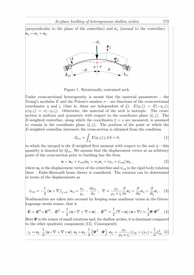
2.1. Pre-buckling state. Figure 1 shows the rotationally restrained arch and theapplied curvilinear coordinate system, which is attached to the E-weighted centerline(or centerline for short). The former has a constant initial radius ρo. The right-handed local base is formed by the unit vectors eξ (tangent to the centerline), eη
In-plane buckling of heterogeneous shallow arches 173
(perpendicular to the plane of the centerline) and eζ (normal to the centerline) –eη = eζ × eξ.
e
e
0
P
f
k kr
Figure 1. Rotationally restrained arch.
Under cross-sectional heterogeneity is meant that the material parameters – theYoung’s modulus E and the Poison’s number ν – are functions of the cross-sectionalcoordinates η and ζ (that is, these are independent of ξ): E(η, ζ) = E(−η, ζ),ν(η, ζ) = ν(−η, ζ). Otherwise, the material of the arch is isotropic. The cross-section is uniform and symmetric with respect to the coordinate plane (ξ, ζ). TheE-weighted centerline, along which the coordinates ξ = s are measured, is assumedto remain in the coordinate plane (ξ, ζ). The position of the point at which theE-weighted centerline intersects the cross-section is obtained from the condition
Qeη =
∫A
E(η, ζ) ζ dA = 0, (1)
in which the integral is the E-weighted first moment with respect to the axis η – thisquantity is denoted by Qeη. We assume that the displacement vector at an arbitrarypoint of the cross-section prior to buckling has the form
u = uo + ψoηζeξ = woeζ + (uo + ψoηζ)eξ , (2)
where uo is the displacement vector of the centerline and ψoη is the rigid body rotationthere – Euler-Bernoulli beam theory is considered. The rotation can be determinedin terms of the displacements as
ψoη = −1
2(u×∇)|ζ=0 · eη =
uoρo− dwo
ds, ∇ =
ρoρo + ζ
∂
∂seξ +
∂
∂ηeη +
∂
∂ζeζ . (3)
Nonlinearities are taken into account by keeping some nonlinear terms in the Green-Lagrange strain tensor, that is
E = EL+EN , EL =1
2(u ◦ ∇+∇ ◦ u) , EN =
1
2(∇ ◦ u)·(u ◦ ∇) ' 1
2Ψ ·ΨT . (4)
Here Ψ is the tensor of small rotations and, for shallow arches, it is dominant comparedto the other quadratic components [15]. Consequently
εξ = eξ ·1
2(u ◦ ∇+∇ ◦ u) ·eξ +eξ ·
1
2
(ΨT · Ψ
)·eξ =
ρoρo + ζ
(εoξ + ζκo)+1
2ψ2oη (5)

174 L. Kiss
is the axial strain at an arbitrary point, where
εoξ =duods
+woρo
, κo =dψoηds
=1
ρo
duods− d2wo
ds2and εm = εoξ +
1
2ψ2oη . (6)
Here εoξ and εm are the linear and the nonlinear axial strain on the centerline, furtherκo is the curvature there.
It is assumed that σξ is much greater than any other element of the second Piola-Kirchhoff stress tensor. Under this condition σξ = Eεξ is the constitutive equation.The E-weighted reduced area AeR, the E-weighted reduced moment of inertia IeRand the E-weighted reduced first moment QeR are defined as
AeR =
∫A
ρoρo + ζ
E(η, ζ) dA '∫A
E(η, ζ) dA = Ae , (7a)
IeR =
∫A
ρoρo + ζ
E(η, ζ)ζ2 dA '∫A
ζ2E(η, ζ)dA = Ieη , (7b)
QeR =
∫A
ρoρo + ζ
E(η, ζ)ζ dA ' 1
ρo
∫A
ζ2E(η, ζ) dA = −Ieηρo. (7c)
With the aid of these quantities and by recalling the kinematic relations (5)-(6), weget the axial force and the bending moment:
N =
∫A
Eεξ dA = AeRεoξ +QeRκo +Ae1
2ψ2oη ≈ Aeεm −
Ieηρoκo , (8)
M =
∫A
Eεξζ dA =
∫A
Eζ
1 + ζρo
dA︸ ︷︷ ︸QeR'−
Ieηρo
εoξ +
∫A
Eζ2
1 + ζρo
dA︸ ︷︷ ︸IeR'Ieη
κo +
∫A
Eζ dA︸ ︷︷ ︸Qeη=0
1
2ψ2oη =
= −Ieη(
d2wods2
+woρ2o
). (9)
With the knowledge of the bending moment we can check – by utilizing (8) and (6)2,3– that
N =Ieηρ2o
(Aeρ
2o
Ieη− 1
)εm −
M
ρo≈ Aeεm −
M
ρo. (10)
2.2. Post-buckling state. Quantities denoted by an asterisk belong to the post-buckling equilibrium state, while the change (increment) between the pre- and post-buckling equilibrium is denoted by a subscript b. (The change from the initial con-figuration to the pre-buckling state is not denoted specifically.) Making use of thisconvention, similarly as before, we can derive the rotation field and the change ofcurvature as
ψ∗oη = ψoη + ψoη b , ψoη b =uobρo− dwob
ds, κ∗o = κo + κo b , κo b =
1
ρo
duobds− d2wob
ds2.
(11)

In-plane buckling of heterogeneous shallow arches 175
As regards the strain increment (assuming∣∣∣ 12ψ2
oη b
∣∣∣ � |ψoηψoη b|, which is generally
accepted in the literature) we have
ε∗ξ =ρo
ρo + ζ
(ε∗oξ + ζκ∗o
)+
1
2
(ψ∗oη)2
= εξ+εξ b, εξ b 'ρo
ρo + ζ(εoξ b + ζκo b)+ψoη bψo η ;
(12a)
εoξ b =duobds
+wobρo
, εmb ' εoξ b + ψoη bψo η . (12b)
Recalling (7), (8), (10) and (12) we can write
N∗ =
∫A
Eε∗ξ dA = N +Nb , Nb = Aeεmb −Ieηρoκob . (13)
In the same way we obtain the increment in the bending moment as
M∗ =
∫A
Eε∗ξζ dA = M +Mb , Mb = −Ieη(
d2wobds2
+wobρ2o
). (14)
Let us assume that
Aeρ2o/Ieη − 1 ≈ Aeρ2o/Ieη = (ρo/ie)
2 = m , ie =√Ieη/Ae . (15)
Here ie is the E-weighted radius of gyration and m is the slenderness ratio of the arch.The latter (heterogeneity) parameter is of particular importance as the computationalresults will significantly depend on it.
With the knowledge of the increment in the bending moment we can check, in thesame way as we did for equation (10), that
Nb =Ieηρ2o
(Aeρ
2o
Ieη− 1
)εmb −
Mb
ρo≈ Aeεmb −
Mb
ρo. (16)
It should be pointed out that Bradford et al. have assumed ρo/(ρo + ζ) = 1 whenexpressing the axial strain and the strain increment at an arbitrary point. Theyhave also neglected the terms M/ρo and Mb/ρo in their corresponding article whenexpressing the axial force and its increment – compare (10) and (16) with (15) and(47) in [17]
We shall change derivatives with respect to s to derivatives with respect to ϕ byusing the following equation:
dn(. . .)
dsn=
1
ρno
dn(. . .)
dϕn= (. . .)
(n), n ∈ Z. (17)
This transformation is carried out, where necessary without a remark.
3. Governing equations
3.1. Equations of the pre-buckling equilibrium. Assuming symmetric loadingand support conditions Figure 1 shows the centerline in the initial configuration (con-tinuous line) and in the pre-buckling equilibrium (dashed line). We shall assume ina more general approach that the arch with a central angle of 2ϑ is subjected to theconcentrated force Pζ at the crown as well as to the arbitrary distributed line load
176 L. Kiss
f = fteξ + fneζ . Moreover, the [left] (right) end of the arch is rotationally restrainedby torsional springs with spring stiffness [kγ`] (kγ r). The principle of virtual work isgiven by∫
V
σξδεξ dV = −Pζ δwo|s=0 − kγ`ψoηδψoη|s(−ϑ) − kγrψoηδψoη|s(ϑ) +
+
∫L
(fnδwo + ftδuo) ds, (18)
where the virtual quantities are preceded by the symbol δ. After substituting thekinematic equations (5) and (6) in terms of the virtual quantities and applying thenformulae (8) and (9) established for the inner forces, the integration by parts theo-rem leads to a form of the principle of virtual work from which, with regard to thearbitrariness of the virtual quantities, we get the equilibrium equations
dN
ds+
1
ρo
[dM
ds−(N +
M
ρo
)ψoη
]+ ft = 0 ,
d
ds
[dM
ds−(N +
M
ρo
)ψoη
]− N
ρo+ fn = 0 .
(19)
It also follows from the principle of virtual work that boundary conditions can beimposed on
N |s(±ϑ) or uo|s(±ϑ) , (20a)[dM
ds−(N +
M
ρo
)ψoη
]∣∣∣∣s(±ϑ)
or wo|s(±ϑ) , (20b)
(M ± kγψoη)|s(±ϑ) or ψoη|s(±ϑ) , (20c)
where it is assumed that kγ` = kγ r = kγ . In addition, the discontinuity condition[dM
ds−(N +
M
ρo
)ψoη
]∣∣∣∣s=+0
−[
dM
ds−(N +
M
ρo
)ψoη
]∣∣∣∣s=−0
− Pζ = 0 (21)
for the shear force at the crown point should also be fulfilled.
In the sequel we assume ft = fn = 0. Upon substitution of equation (6) intoequation (19)1 we get
d
ds(Aeεm)− 1
ρo(Aeεmψoη) = 0 . (22)
Let us now neglect the quadratic term εmψoη. Consequently, we arrive at
dεmds' dεoξ
ds= 0 → εm ' εoξ = constant, (23)
which shows, depending on which theory is applied, that the nonlinear/linear strainon the centerline is constant.
If we introduce (3) and (6)1,3 into the expression ρoεm
(1 + ψ
(1)oη
)we arrive at the
following result (the quadratic term is neglected when that is compared to the others):
In-plane buckling of heterogeneous shallow arches 177
ρoεm
(1 + ψ(1)
oη
)= ρoεm
[1 +
1
ρo
(u(1)o − w(2)
o
)]=
= ρoεm
[1 +
1
ρo
(ρoεm − wo −
1
2ψ2oηρo − w(2)
o
)]≈
≈ ρoεm(1 + εm)︸ ︷︷ ︸≈1
− εm(wo + w(2)
o
)≈ ρoεm − εm
(w(2)o + wo
). (24)
Substitute now formulae (9) and (10) into (19)2 and take equations (23) and (24) intoaccount. After some manipulations we have
W (4)o +
(χ2 + 1
)W (2)o + χ2Wo = χ2 − 1 , χ2 = 1−mεm . (25)
Here and in the sequel Wo = wo/ρo and Uo = uo/ρo are dimensionless displacements.Equation (25) can be compared with the equation Bradford et al. have used in theirseries of articles published recently on stability problems of shallow arches. Thisequation is of the form
W (4)o + (χ2 − 1)W (2)
o = χ2 − 1. (26)
Equation (25) includes less neglects than that derived by Bradford et al. – see, e.g.,[15], [17].
3.2. Equations of the post-buckling equilibrium. The principle of virtual workfor the buckled equilibrium configuration assumes the form∫
V
σ∗ξδε∗ξ dV = −P ∗ζ δw∗o |s=0 − kγ`ψ
∗oηδψ
∗oη
∣∣s(−ϑ) − kγrψ
∗oηδψ
∗oη
∣∣s(ϑ)
+
+
∫L
(f∗nδw∗o + f∗t δu
∗o) ds . (27)
By repeating the line of thought leading to (19),(20) and taking into account that (a)the principle of virtual work should be fulfilled in the pre-buckling state; (b) Pζb = 0and kγ` = kγ r = kγ the principle of virtual work yields
dNbds
+1
ρo
dMb
ds− 1
ρo
(N +
M
ρo
)ψoη b −
1
ρo
(Nb +
Mb
ρo
)ψoη b + ftb = 0 , (28a)
d2Mb
ds2− Nbρo− d
ds
[(N +Nb +
M +Mb
ρo
)ψoη b +
(Nb +
Mb
ρo
)ψoη
]+ fnb = 0,
(28b)
which govern the post-buckling equilibrium. For the buckled configuration, boundaryconditions can be prescribed on the following quantities:
Nb|s(±ϑ) or uob|s(±ϑ) ,
(29a)[dMb
ds−(N +Nb +
M +Mb
ρo
)ψoη b −
(Nb +
Mb
ρo
)ψoη
]∣∣∣∣s(±ϑ)
or wob|s(±ϑ) ,
(29b)

178 L. Kiss
(Mb ± kγψoη)|s(±ϑ) or ψoη b|s(±ϑ) .(29c)
In the forthcoming it is assumed that ftb = fnb = 0. Observe that, apart fromthe last but one term, (28a) formally coincides with (19)1. However, since the termmentioned is quadratic in the increment, it can be neglected with a good accuracy.Therefore repeating now a similar line of thought leading to (23), we obtain that thestrain increment is constant:
d
ds(Aeεmb)−
1
ρo(Aeεmψoηb)︸ ︷︷ ︸
it can also be neglected
= 0 ⇒ εmb ' εoξ b = constant . (30)
If we (a) take into account that ε(1)m = ε
(1)mb = 0; (b) substitute Mb from (14) and
(c) utilize that
mρoεmb
(1 + ψ(1)
oη
)' mρoεmb
[1− 1
ρo
(w(2)o + wo
)]= mρoεmb −mεmb
(w(2)o + wo
)(this relation can be set up in the same way as (24)) then, after some manipulations,(28b) results in
W(4)ob + (χ2 + 1)W
(2)ob + χ2Wob = mεmb
[1−
(W (2)o +Wo
)]. (31)
This equation is again comparable with the outcome derived by Bradford et al. –e.g., [15], [17] – that is
W(4)ob + (χ2 − 1)W
(2)ob = mεmb
[1−W (2)
o
]. (32)
4. Solution for the pre-buckling state
The general solution satisfying (25) for the dimensionless normal displacement is ofthe form
Wo(ϕ) =χ2 − 1
χ2+A1 cosϕ+A2 sinϕ− A3
χ2cosχϕ− A4
χ2sinχϕ, (33)
in which Ai (i = 1, . . . , 4) are integration constants. Since all the geometry, the loa-
Table 1. Boundary conditions for the rotationally restrained arch.
Boundary conditions
Crown point Right end
ψoη |ϕ=+0 = 0→ W(1)o
∣∣∣ϕ=+0
= 0 Wo|ϕ=ϑ = 0[−dM
ds+Pζ2
]ϕ=+0
= 0→ W(3)o
∣∣∣ϕ=+0
= Pϑ
[M + kγψo η ]|ϕ=ϑ= 0→[W
(2)o + SW (1)
o
]∣∣∣ϕ=ϑ
= 0
ding and the supports are symmetric, it is sufficient to consider a half of the arch as thepre-buckling shape is also symmetric. To determine the integration constants, we shalluse the boundary conditions (BCs) presented in Table 1 – P = −Pζρ2oϑ/2Ieη is thedimensionless load and S = ρokγ/Ieη is the dimensionless stiffness of the restraints.

In-plane buckling of heterogeneous shallow arches 179
For the sake of brevity let us introduce the constant
a =(χ2 − 1
)cosϑ cosχϑ− S (sinϑ cosχϑ− χ cosϑ sinχϑ) . (34)
Solution (33) satisfies the boundary conditions if
A1 = A11 +PϑA12 =
(1− χ2
)(χ cosχϑ+ S sinχϑ)
χa+
+
(1− χ2
)sinϑ cosχϑ− S (cosϑ cosχϑ+ χ sinϑ sinχϑ− 1)
(χ2 − 1) a
Pϑ, (35a)
A2 =1
(χ2 − 1)
Pϑ
= A22Pϑ
; (35b)
A3 = A31 +PϑA32 =
cosϑ+ S sinϑ
−a+
+χ[(χ2 − 1
)cosϑ sinχϑ− S (sinϑ sinχϑ+ χ cosϑ cosχϑ− χ)
]− (χ2 − 1) a
Pϑ, (35c)
A4 =χ
(χ2 − 1)
Pϑ
= A42Pϑ. (35d)
If [S = 0] (S → ∞) we get back the results valid for [pinned-pinned] (fixed-fixed)arches – see [20], [21]. The radial displacement for the whole arch is given by
Wo =χ2 − 1
χ2+A11 cosϕ− A31
χ2cosχϕ+
+
(A12 cosϕ+A22H sinϕ− A32
χ2cosχϕ− A42
χ2H sinχϕ
)Pϑ
; (36)
in which H = H(ϕ) = 1 if ϕ > 0 and H = H(ϕ) = −1 if ϕ < 0. The rotation field(by neglecting the effects of the tangential displacement due to the shallowness) is
ψoη ' −W (1)o = B11 sinϕ+B31 sinχϕ+
+ (B12 sinϕ+B22H cosϕ+B32 sinχϕ+B42H cosχϕ)Pϑ
; (37)
where the new constants are
B11 = A11 , B12 = A12 , B22 = −A22 , B31 = −A31
χ, B32 = −A32
χ, B42 =
A42
χ.
Because the strain on the centerline is constant, based on (23), the mathematicalaverage of the strain, i.e., the strain itself, is given by
εm =1
ϑ
∫ ϑ
0
εmdϕ =1
ϑ
∫ ϑ
0
(εoξ +
1
2ψ2oη
)dϕ =
1
ϑ
∫ ϑ
0
(U (1)o +Wo +
1
2ψ2oη
)dϕ;
(38)where
1
ϑ
∫ ϑ
0
U (1)o dϕ = Uo|ϑ0 = 0. (39)
180 L. Kiss
Equation (38) results in the
I2P2 + I1P + I0 − εm = 0 , Ij(m,ϑ, χ,S) ∈ R, j = 0, 1, 2 (40)
quadratic formula for the dimensionless force, in which the coefficients Ij can beobtained in a closed form – see Appendix A.1 for details.
5. Solutions for the post-buckling state
5.1. Differential equations, which govern the problem. Substitution of thesolution (36) into the post-buckling equilibrium equation (31) yields
W(4)ob + (1 + χ2)W
(2)ob + χ2Wob = −mεmb
1− χ2
χ2
(1
1− χ2+A3 cosχϕ+A4 sinχϕ
).
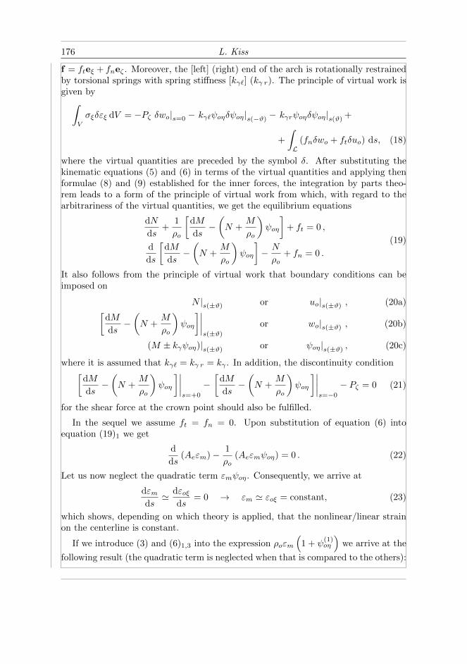
(41)In general, there are two possibilities regarding the buckled equilibrium of the arch[15]. When the strain increment εmb is constant but not equal to zero, the problemis governed by the above relation and the buckled shape is symmetric. However,it is also possible that the arch buckles antisymmetrically with no strain increment(εmb = 0). Then the phenomenon is described by the
W(4)ob + (1 + χ2)W
(2)ob + χ2Wob = 0 (42)
homogeneous differential equation. The mathematical average of the strain incre-ment, that is, the strain increment itself can be determined by using the kinematicalequations (3), (10) and (12b) under the assumption that the effect of the normaldisplacement is again negligible when calculating the rotation increment:
εmb '1
2ϑ
∫ ϑ
−ϑ(εoξ b+ψoη bψoη) dϕ=
1
2ϑ
∫ ϑ
−ϑ
[U
(1)ob +Wob+
(Uob−W (1)
ob
)(Uo−W (1)
o
)]dϕ ≈
≈ 1
2ϑ
∫ ϑ
−ϑ
(Wob +W
(1)ob W
(1)o
)dϕ. (43)
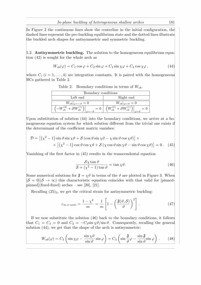
It will later be shown that antisymmetric shape belongs to bifurcation buckling, whilein the case of a snap-through (or limit point) buckling the shape of the arch is alwayssymmetric.
Figure 2. Antisymmetric and symmetric buckling shapes.
In-plane buckling of heterogeneous shallow arches 181
In Figure 2 the continuous lines show the centerline in the initial configuration, thedashed lines represent the pre-buckling equilibrium state and the dotted lines illustratethe buckled arch shapes for antisymmetric and symmetric buckling.
5.2. Antisymmetric buckling. The solution to the homogeneous equilibrium equa-tion (42) is sought for the whole arch as
Wob(ϕ) = C1 cosϕ+ C2 sinϕ+ C3 sinχϕ+ C4 cosχϕ , (44)
where Ci (i = 1, . . . , 4) are integration constants. It is paired with the homogeneousBCs gathered in Table 2.
Table 2. Boundary conditions in terms of Wob.
Boundary conditions
Left end Right end
Wob|ϕ=−ϑ = 0 Wob|ϕ=ϑ = 0(−W (2)
ob + SW (1)ob
)∣∣∣ϕ=−ϑ
= 0(W
(2)ob + SW (1)
ob
)∣∣∣ϕ=ϑ
= 0
Upon substitution of solution (44) into the boundary conditions, we arrive at a ho-mogeneous equation system for which solution different from the trivial one exists ifthe determinant of the coefficient matrix vanishes:
D =[(χ2 − 1
)sinϑ sinχϑ+ S (cosϑ sinχϑ− χ sinϑ cosχϑ)
]×
×[(χ2 − 1
)cosϑ cosχϑ+ S (χ cosϑ sinχϑ− sinϑ cosχϑ)
]= 0 . (45)
Vanishing of the first factor in (45) results in the transcendental equation
Sχ tanϑ
S + (χ2 − 1) tanϑ= tanχϑ. (46)
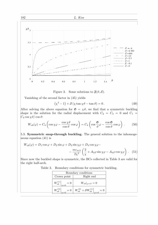
Some numerical solutions for F = χϑ in terms of the ϑ are plotted in Figure 3. When[S = 0](S → ∞) this characteristic equation coincides with that valid for [pinned-pinned](fixed-fixed) arches – see [20], [21].
Recalling (25)2, we get the critical strain for antisymmetric buckling:
εmcr anti =1− χ2
m=
1
m
[1−
(F(ϑ,S)
ϑ
)2]. (47)
If we now substitute the solution (46) back to the boundary conditions, it followsthat C1 = C4 = 0 and C2 = −C3sinχϑ/sinϑ. Consequently, recalling the generalsolution (44), we get that the shape of the arch is antisymmetric:
Wob(ϕ) = C3
(sinχϕ− sinχϑ
sinϑsinϕ
)= C3
(sin
F
ϑϕ− sinF
sinϑsinϕ
). (48)
182 L. Kiss
Figure 3. Some solutions to F(ϑ,S).
Vanishing of the second factor in (45) yields(χ2 − 1
)+ S (χ tanχϑ− tanϑ) = 0 . (49)
After solving the above equation for G = χϑ, we find that a symmetric bucklingshape is the solution for the radial displacement with C2 = C3 = 0 and C1 =C4 cosχϑ/ cosϑ:
Wob(ϕ) = C4
(cosχϕ− cosχϑ
cosϑcosϕ
)= C4
(cos
G
ϑϕ− cosG
cosϑcosϕ
). (50)
5.3. Symmetric snap-through buckling. The general solution to the inhomoge-neous equation (41) is
Wob(ϕ) = D1 cosϕ+D2 sinϕ+D3 sinχϕ+D4 cosχϕ−
− mεmb
2χ3
(2
χ+A3ϕ sinχϕ−A4ϕ cosχϕ
). (51)
Since now the buckled shape is symmetric, the BCs collected in Table 3 are valid forthe right half-arch.
Table 3. Boundary conditions for symmetric buckling.
Boundary conditions
Crown point Right end
W(1)ob
∣∣∣ϕ=0
= 0 Wob|ϕ=ϑ = 0
W(3)ob
∣∣∣ϕ=0
= 0 W(2)ob + SW (1)
ob
∣∣∣ϕ=ϑ
= 0
In-plane buckling of heterogeneous shallow arches 183
Upon substitution of solution (51) into the boundary conditions, we get a system oflinear equations from which
D1 = εmb
(D11 + D12
Pϑ
)=
= εmbm
χ3a
{A31
[χ cos2 χϑ+ 0.5S (ϑχ+ cosχϑ sinχϑ)
]+ (χ cosχϑ+ S sinχϑ)
}+
+ εmbm
2χ3 (1− χ2) a
{A32
(1− χ2
) [2χ cos2 χϑ+ S (ϑχ+ cosχϑ sinχϑ)
]+
+A42
[2χ(1− χ2
)(sinχϑ− χ sinϑ) cosχϑ+
+S(2χ2 cosϑ cosχϑ+ 2χ3 sinϑ sinχϑ− 3χ2 + 1 +
(χ2 − 1
)cos2 χϑ
)]}Pϑ, (52a)
D2 = εmbD22Pϑ
= εmbmA42
(χ2 − 1)χ
Pϑ, D3 = εmbD32
Pϑ
= εmbA42m
(3χ2 − 1
)2χ4 (1− χ2)
Pϑ,
(52b)
D4 = εmb
(D41 + D42
Pϑ
)=
= εmbm cosϑ
−2χ4a
{2 (1 + S tanϑ) +A31χ
[2χ− ϑ
(χ2 − 1
)tanχϑ +
+ S (ϑ tanϑ tanχϑ+ tanχϑ+ χϑ)] cosχϑ
}+
+ εmbm
2χ4 (χ2 − 1) a
{A32χ
(1− χ2
) [(2χ− ϑ
(χ2 − 1
)tanχϑ
)+
+S (ϑ tanϑ tanχϑ+ tanχϑ+ χϑ)] cosϑ cosχϑ+
+A42
[(1− χ2
)2(tanχϑ− χϑ) cosϑ cosχϑ+ S
[2χ3 (1− cosϑ cosχϑ) +
+(1− χ2
)ϑχ (χ tanχϑ− tanϑ) cosϑ cosχϑ+
(1− 3χ2
)sinϑ sinχϑ
] ]}Pϑ
(52c)
are the integration constants Di (i = 1, . . . , 4). We remark that the constants D11,
D12, D22, D32, D41 and D42 can be read off equations (52).
For the sake of brevity, we manipulate the particular solution to (51) into thefollowing form:
Wob part = −εmbm
2χ3
[2
χ+
(A31 +A32
Pϑ
)ϕ sinχϕ−A42ϕ cosχϕ
Pϑ
]=
= εmb
[−mχ4− A31m
2χ3ϕ sinχϕ+
(−A32m
2χ3ϕ sinχϕ+
A42m
2χ3ϕ cosχϕ
)Pϑ
]=
= εmb
[D01 + D51ϕ sinχϕ+
(D52ϕ sinχϕ+ D62ϕ cosχϕ
) Pϑ
], (53a)
184 L. Kiss
where
D01 = −mχ4
, D51 = −A31m
2χ3, D52 = −A32m
2χ3, D62 =
A42m
2χ3. (53b)
With the knowledge of the integration constants
Wob(ϕ) = εmb
[D01 + D11 cosϕ+ D41 cosχϕ+ D51ϕ sinχϕ+
+(D12 cosϕ+ D22H sinϕ+ D32H sinχϕ+ D42 cosχϕ+
+D52ϕ sinχϕ+ D62Hϕ cosχϕ) Pϑ
](54)
is the solution for the complete arch. The increment in the rotation field for shallowarches is given by
− ψoη b 'W (1)ob = εmb
[E11 sinϕ+ E41 sinχϕ+ E51ϕ cosχϕ+
+ (E12 sinϕ+ E22 cosϕ+ E32 cosχϕ+ E42 sinχϕ+
E52ϕ cosχϕ+ E62ϕ sinχϕ)Pϑ
], (55)
where
E11 = −D11 , E41 = D51 − D41χ , E51 = D51χ , E12 = −D12 , E22 = D22H ,
E32 = D32Hχ+ D62H , E42 = D52 − D42χ , E52 = D52 , E62 = −D62H .
(56)We can now calculate the mathematical average of the strain increment for the righthalf arch on the basis of (43). We get
1 =1
ϑεmb
∫ ϑ
0
(U
(1)ob +Wob +W (1)
o W(1)ob
)dϕ = J2P2 + J1P + J0, (57)
where the right side is also independent of εmb. Formulae for the coefficients (integrals)J0, J1 and J2 are presented in Appendix A.1. Though the corresponding integralscan be given in a closed form, these are very long and are therefore omitted.
6. Computational results
6.1. What to compute? In this section results are presented for four different mag-nitudes of the parameter m. At first, we investigate how the spring stiffness affectsthe endpoints of the typical buckling intervals. Then the critical loads are calculated.The results are comparable with those obtained by Bradford et al. in [15] and [17]using more neglects but, due to this fact, arriving at analytical solutions. WhenS = 0 and S → ∞ our results – since they are based on a similar mechanical model –coincide with those valid both for pinned-pinned [20] and for fixed-fixed [21] arches.

In-plane buckling of heterogeneous shallow arches 185
6.2. Limits for the characteristic buckling intervals. There are four intervals ofinterest regarding the buckling behavior of symmetrically supported shallow arches.For a given ϑ, the endpoints of these intervals are functions of m, χ(εm) and S.The lower limit of antisymmetric buckling can be obtained from the condition thatthe discriminant of (40) should be real when the antisymmetric critical strain (46) issubstituted, consequently inequality[
I21 − 4I2(I0 − εmcr anti)]∣∣χϑ=F
≥ 0 (58)
should be fulfilled. We remark that when the spring stiffness is zero – i.e. the arch ispinned-pinned – instead of using the exact solution we assumed that F = π−10−4. Itis also possible in certain cases that a real antisymmetric solution vanishes, so there isan upper limit also in the investigated ϑ = 0 . . . 1.5 range. The upper limit is obtainedby using an algorithm which monitors at what value of S there exists no real solutionany longer if χϑ = F.
When evaluating the critical antisymmetric and symmetric buckling loads againstthe geometry of the arch, we find that these two curves sometimes intersect each other.This intersection point varies with S. There is a switch between the symmetric andantisymmetric buckling modes at the intersection point as it is shown in Section 6.4.Prior to the intersection, the symmetric buckling shape governs. However, after thisintersection, the bifurcation point is located before the limit point of the correspondingprimary equilibrium path, which means that antisymmetric buckling occurs first. (Tobetter understand the meaning of limit point see Figure 12). This switch can be foundwhen (40) and (57) are equal at χϑ = F with all the other parameters being the same:[
I2P2 + I1P + I0 − εm]∣∣
F,m,S,P =[J2P2 + J1P + J0
]∣∣F,m,S,P . (59)
Finally, the lower endpoint for symmetric buckling, below which there is no buck-ling at all, is obtained by substituting the lowest symmetric solution (49) into thepre-buckling averaged strain (40) when the discriminant is set to zero:[
I21 − 4I2(I0 − εmcr sym)]∣∣χϑ=G
= 0. (60)
Now we turn the attention to the evaluation. Choosing m = 1 000, Figure 4 showsthe effects of the dimensionless spring stiffness in terms of the semi-vertex angle.When S = 0, we get back the results valid for a pinned-pinned arch. Thus, whenϑ ≤ 0.347 there is no buckling – see the range denoted by (I). Then, up until ϑ = 0.5,only symmetric limit point buckling can occur at the right loading level (II). Eventhough a bifurcation point (and therefore the possibility of antisymmetric buckling)appears when further increasing ϑ (III), still the symmetric shape is the dominantup until the intersection point of the symmetric and antisymmetric buckling curvesat ϑ = 0.553. At this point the buckling loads and strains are the same for symmetricand antisymmetric buckling and it holds a switch between the buckling types sinceabove it (IV ) the bifurcation point is located on the stabile branch of the primary

186 L. Kiss
Figure 4. Typical buckling ranges when m = 1 000.
equilibrium path as it will be shown later. Apart from the range limits, there are noany other differences as long as S ≤4.2. Passing this value results in the disappearanceof the intersection point of the buckling curves, therefore antisymmetric buckling isonly possible after symmetric buckling. Another limit of importance is S = 7.6, sinceabove that, the bifurcation point vanishes. It can also be seen that as S approaches toinfinity from below – i.e. the arch becomes fixed – the switch between no buckling andsymmetric buckling can be found at ϑ = 0.606. The results when [S = 0] (S → ∞)are in a complete accord with what have been achieved in [20], [21]. This statementis valid for all the forthcoming results as well.
Figure 5. Typical buckling ranges when m = 10 000.
The behavior of arches with m = 10 000 is very similar to the former description– see Figure 5. This time an intersection point can be found up until S = 6.6 andan upper limit for antisymmetric buckling until S ≤ 33.3. So these points show an
In-plane buckling of heterogeneous shallow arches 187
increase in S as m is increased. It is also noticeable that increasing m yields a decreasein all the typical buckling endpoints in ϑ.
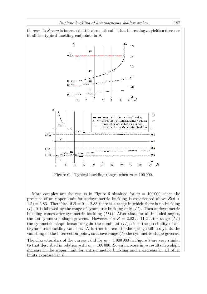
Figure 6. Typical buckling ranges when m = 100 000.
More complex are the results in Figure 6 obtained for m = 100 000, since thepresence of an upper limit for antisymmetric buckling is experienced above S(ϑ <1.5) = 2.83. Therefore, if S = 0 . . . 2.83 there is a range in which there is no buckling(I). It is followed by the range of symmetric buckling only (II). Then antisymmetricbuckling comes after symmetric buckling (III). After that, for all included angles,the antisymmetric shape governs. However, for S = 2.83 . . . 11.2 after range (IV )the symmetric shape becomes again the dominant (II), since the possibility of an-tisymmetric buckling vanishes. A further increase in the spring stiffness yields thevanishing of the intersection point, so above range (I) the symmetric shape governs.
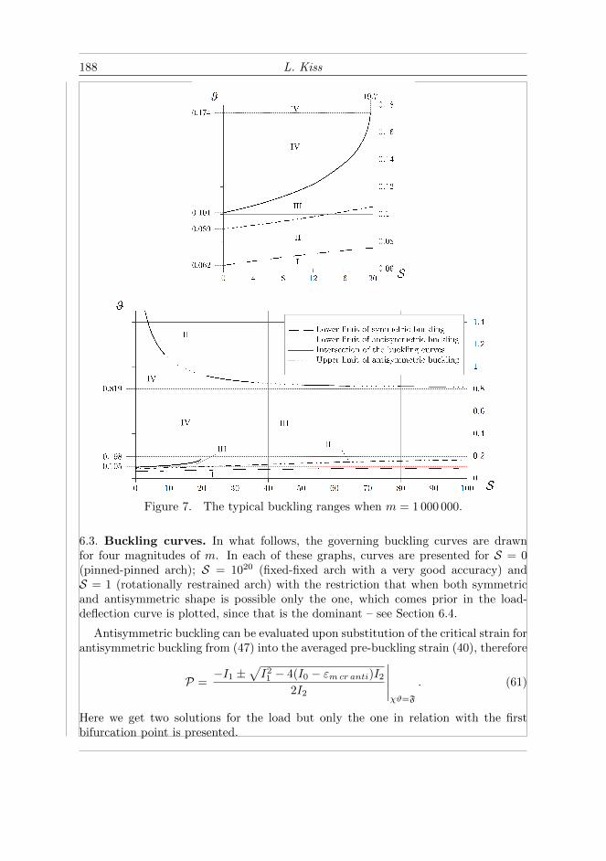
The characteristics of the curves valid for m = 1 000 000 in Figure 7 are very similarto that described in relation with m = 100 000. So an increase in m results in a slightincrease in the upper limit for antisymmetric buckling and a decrease in all otherlimits expressed in ϑ.
188 L. Kiss
Figure 7. The typical buckling ranges when m = 1 000 000.
6.3. Buckling curves. In what follows, the governing buckling curves are drawnfor four magnitudes of m. In each of these graphs, curves are presented for S = 0(pinned-pinned arch); S = 1020 (fixed-fixed arch with a very good accuracy) andS = 1 (rotationally restrained arch) with the restriction that when both symmetricand antisymmetric shape is possible only the one, which comes prior in the load-deflection curve is plotted, since that is the dominant – see Section 6.4.
Antisymmetric buckling can be evaluated upon substitution of the critical strain forantisymmetric buckling from (47) into the averaged pre-buckling strain (40), therefore
P =−I1 ±
√I21 − 4(I0 − εmcr anti)I2
2I2
∣∣∣∣∣χϑ=F
. (61)
Here we get two solutions for the load but only the one in relation with the firstbifurcation point is presented.
In-plane buckling of heterogeneous shallow arches 189
As for symmetric buckling we have two unknowns – the force and the critical strain.We also have two equations – one obtained from the averaged pre- (40) and one fromthe averaged post-buckling strain (57). Solving these simultaneously[
I2P2 + I1P + I0 − εm]∣∣χ,ϑ,S,m =
[J2P2 + J1P + J0
]∣∣χ,ϑ,S,m (62)
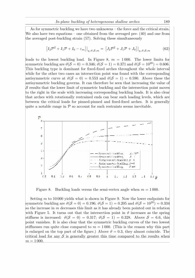
leads to the lowest buckling load. In Figure 8, m = 1 000. The lower limits forsymmetric buckling are ϑ(S = 0) = 0.346; ϑ(S = 1) = 0.371 and ϑ(S = 1020) = 0.606.This buckling type is dominant for fixed-fixed arches throughout the whole intervalwhile for the other two cases an intersection point was found with the correspondingantisymmetric curve at ϑ(S = 0) = 0.553 and ϑ(S = 1) = 0.590. Above these theantisymmetric buckling governs. It can therefore be seen that increasing the value ofS results that the lower limit of symmetric buckling and the intersection point movesto the right in the scale with increasing corresponding buckling loads. It is also clearthat arches with rotationally restrained ends can bear such loading levels, which arebetween the critical loads for pinned-pinned and fixed-fixed arches. It is generallyquite a notable range in P so account for such restraints seems inevitable.
Figure 8. Buckling loads versus the semi-vertex angle when m = 1 000.
Setting m to 10 000 yields what is shown in Figure 9. Now the lower endpoints forsymmetric buckling are ϑ(S = 0) = 0.196; ϑ(S = 1) = 0.205 and ϑ(S = 1020) = 0.334so the increase in m decreases this limit as it has already been pointed out in relationwith Figure 5. It turns out that the intersection point in ϑ increases as the springstiffness is increased: ϑ(S = 0) = 0.317; ϑ(S = 1) = 0.328. Above S = 6.6, thispoint vanishes. It is also clear that the symmetric buckling curves of the two loweststiffnesses run quite close compared to m = 1 000. (This is the reason why this partis enlarged on the top part of the figure.) Above ϑ = 0.3, they almost coincide. Thecritical load for any S is generally greater this time compared to the results whenm = 1 000.

190 L. Kiss
0.2 0.25 0.3 0.35 0.4
1.5
2
2.5
3
3.5
4
4.5
5
5.5
P
Figure 9. Buckling loads versus the semi-vertex angle when m = 10 000.
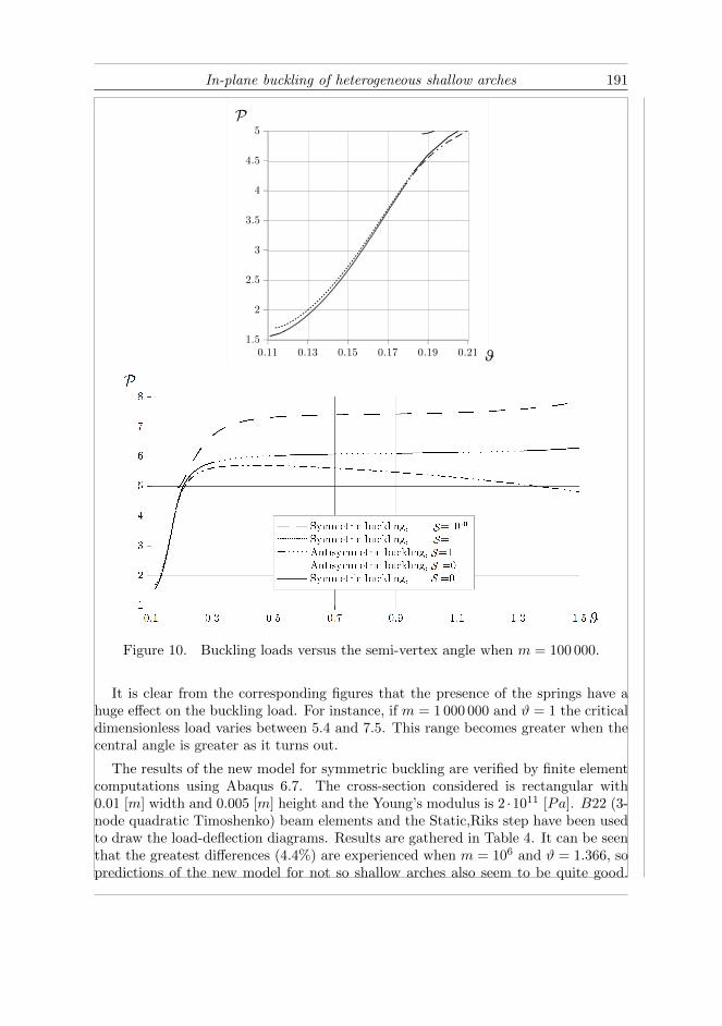
In Figure 10, m is 100 000. The lower limit of symmetric buckling happens todecrease further but slowly: ϑ(S = 0) = 0.111; ϑ(S = 1) = 0.113 and ϑ(S = 1020) =0.187, while the intersection points occur at ϑ(S = 0) = 0.179; ϑ(S = 1) = 0.182.This time the symmetric curves are again closer to each other and the starting pointsof all the curves are closer to the origin.
With m = 1 000 000, we find that ϑ(S = 0) = 0.062; ϑ(S = 1) = 0.063 andϑ(S = 1020) = 0.105 are the lower limits for symmetric buckling and ϑ(S = 0) =0.101; ϑ(S = 1) = 0.102 for the intersection point. This intersection point exists untilS = 19.7. The symmetric buckling curves for the two lowest stiffnesses coincide witha very good accuracy in their quite narrow interval in ϑ. Generally, the differencescompared to m = 100 000 are not that relevant when moving from m = 1 000 tom = 10 000.
In-plane buckling of heterogeneous shallow arches 191
0.11 0.13 0.15 0.17 0.19 0.21
1.5
2
2.5
3
3.5
4
4.5
5
P
Figure 10. Buckling loads versus the semi-vertex angle when m = 100 000.
It is clear from the corresponding figures that the presence of the springs have ahuge effect on the buckling load. For instance, if m = 1 000 000 and ϑ = 1 the criticaldimensionless load varies between 5.4 and 7.5. This range becomes greater when thecentral angle is greater as it turns out.
The results of the new model for symmetric buckling are verified by finite elementcomputations using Abaqus 6.7. The cross-section considered is rectangular with0.01 [m] width and 0.005 [m] height and the Young’s modulus is 2 ·1011 [Pa]. B22 (3-node quadratic Timoshenko) beam elements and the Static,Riks step have been usedto draw the load-deflection diagrams. Results are gathered in Table 4. It can be seenthat the greatest differences (4.4%) are experienced when m = 106 and ϑ = 1.366, sopredictions of the new model for not so shallow arches also seem to be quite good.
192 L. Kiss
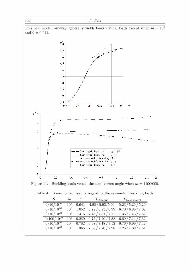
This new model, anyway, generally yields lower critical loads except when m = 103
and ϑ = 0.641.
Figure 11. Buckling loads versus the semi-vertex angle when m = 1 000 000.
Table 4. Some control results regarding the symmetric buckling loads.
S m ϑ PAbaqus PNew model
0/10/1020 103 0.641 4.98 / 5.03/5.09 5.23 / 5.26 / 5.290/10/1020 103 1.052 6.78 / 6.83 / 6.99 6.70 / 6.86 / 7.090/10/1020 103 1.416 7.48 / 7.51 / 7.71 7.36 / 7.43 / 7.620/100/1020 106 0.289 6.75 / 7.20 / 7.38 6.69 / 7.14 / 7.320/10/1020 106 0.782 6.98 / 7.18 / 7.52 6.76 / 6.99 / 7.420/10/1020 106 1.366 7.58 / 7.70 / 7.98 7.26 / 7.39 / 7.64
In-plane buckling of heterogeneous shallow arches 193
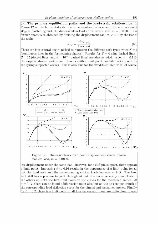
6.4. The primary equilibrium paths and the load-strain relationships. InFigure 12 on the horizontal axis, the dimensionless displacement of the crown pointWoC is plotted against the dimensionless load P for arches with m = 100 000. Theformer quantity is obtained by dividing the displacement (36) at ϕ = 0 by the rise ofthe arch:
WoC =−Wo|ϕ=0
1− cosϑ. (63)
There are four central angles picked to represent the different path types when S = 1(continuous lines in the forthcoming figures). Results for S = 0 (fine dashed lines),S = 15 (dotted lines) and S = 1020 (dashed lines) are also included. When ϑ = 0.113,the slope is always positive and there is neither limit point nor bifurcation point forthe spring supported arches. This is also true for the fixed-fixed arch with, of course,
Figure 12. Dimensionless crown point displacement versus dimen-sionless load, m = 100 000.
less displacement under the same load. However, for a stiff pin support, there appearsa limit point. Increasing ϑ to 0.16 results in the appearance of a limit point for allbut the fixed arch and the corresponding critical loads increase with S. The fixedarch still has a positive tangent throughout but this curve generally runs closer tothe others up until the first limit point on the curves for the restrained arches. Atϑ = 0.17, there can be found a bifurcation point also but on the descending branch ofthe corresponding load-deflection curve for the pinned and restrained arches. Finally,for ϑ = 0.2, there is a limit point in all four curves and these are quite close to each
194 L. Kiss
other as well as all the first stabile branches. This time, and above this central angle,the two picked rotationally restrained and the pinned arches buckle antisymmetricallyfirst, as the bifurcation point is located on the stabile branch, while fixed arches mightstill buckle symmetrically only.
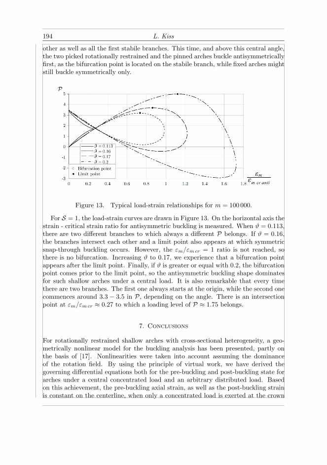
Figure 13. Typical load-strain relationships for m = 100 000.
For S = 1, the load-strain curves are drawn in Figure 13. On the horizontal axis thestrain - critical strain ratio for antisymmetric buckling is measured. When ϑ = 0.113,there are two different branches to which always a different P belongs. If ϑ = 0.16,the branches intersect each other and a limit point also appears at which symmetricsnap-through buckling occurs. However, the εm/εmcr = 1 ratio is not reached, sothere is no bifurcation. Increasing ϑ to 0.17, we experience that a bifurcation pointappears after the limit point. Finally, if ϑ is greater or equal with 0.2, the bifurcationpoint comes prior to the limit point, so the antisymmetric buckling shape dominatesfor such shallow arches under a central load. It is also remarkable that every timethere are two branches. The first one always starts at the origin, while the second onecommences around 3.3 − 3.5 in P, depending on the angle. There is an intersectionpoint at εm/εmcr ≈ 0.27 to which a loading level of P ≈ 1.75 belongs.
7. Conclusions
For rotationally restrained shallow arches with cross-sectional heterogeneity, a geo-metrically nonlinear model for the buckling analysis has been presented, partly onthe basis of [17]. Nonlinearities were taken into account assuming the dominanceof the rotation field. By using the principle of virtual work, we have derived thegoverning differential equations both for the pre-buckling and post-buckling state forarches under a central concentrated load and an arbitrary distributed load. Basedon this achievement, the pre-buckling axial strain, as well as the post-buckling strainis constant on the centerline, when only a concentrated load is exerted at the crown
In-plane buckling of heterogeneous shallow arches 195
point. Heterogeneity appears in the formulation through the parameter χ(m). Theequations of static equilibrium posses less neglects than the model derived and solvedby Bradford et al. – see e.g., [15]; [17]. For this reason, the results computed by usingthe current model are more accurate even for greater central angles as well when theyare compared to the previously cited articles. It should also be mentioned that for therotation field the effect of the tangential displacement is neglected, which can causeerroneous predictions for deeper arches.
The evaluation process of the results are based on what Bradford et al. have usedin their series of articles. We have presented how the different buckling limits andranges are affected by the spring stiffness. It turns out that symmetrically supportedshallow arches under a central load can buckle in an antisymmetric bifurcation modewith no strain increment at the moment of the stability loss, and in a symmetricsnap-through mode, when there is a buckling strain. We have found, in an agreementwith the earlier results, that an increase in S results in an increase of the typicalbuckling limits for any fixed m. However, as m increases, those limits show a decrease.Evaluation of the critical loads for three different spring stiffness is carried out. IfS = 0 and S → ∞, we retrieved the results valid for pinned-pinned and fixed-fixedarches – see [20], [21]. The rotational restraints can have a considerable effect on thecritical load a shallow arch can bear. For the same arches, but with different springstiffnesses, the maximum difference between the critical loads can reach up to 25%when ϑ ≤ 0.8 and up to 57% for greater central angles. The load-deflection curvesare also affected by the rotational restraints as it has been presented.
Acknowledgements. This research was supported by the European Union and theState of Hungary, co-financed by the European Social Fund in the framework of
TAMOP 4.2.4.A/2-11-1-2012-0001 ’National Excellence Program’.
The author would also like to express his gratitude to the unknown reviewers for theirvaluable and constructive comments.
Appendix A.1. Detailed manipulations
Calculation of the pre-buckling averaged strain. Integral (38) is divided into two parts. Thefirst part is
1
ϑ
∫ ϑ
0
Wo dϕ = Ia + IbP,
where
Ia =1
ϑ
∫ ϑ
0
(χ2 − 1
χ2+A11 cosϕ− A31
χ2cosχϕ
)dϕ =
χ2 − 1
χ2+A11
sinϑ
ϑ− A31
χ3
sinχϑ
ϑ,
(A.1)
Ib =1
ϑ2
∫ ϑ
0
(A12 cosϕ+A22 sinϕ− A32
χ2cosχϕ− A42
χ2sinχϕ
)dϕ =
196 L. Kiss
=1
ϑ2
(A12 sinϑ−A22 cosϑ−A32
sinχϑ
χ3+A42
cosχϑ
χ3+A22 −
A42
χ3
). (A.2)
The other part is of the form
1
ϑ
∫ ϑ
0
1
2ψ2oηdϕ = Ic + IdP + IeP2 . (A.3)
Here
Ic =1
2ϑ
∫ ϑ
0
(B11 sinϕ+B31 sinχϕ)2 dϕ =−1
8ϑχ (1− χ2)×
×[B2
11χ (sin 2ϑ−2ϑ)+8B11B31χ (sinχϑ cosϑ−χ sinϑ cosχϑ)
(1−χ2)+B2
31 (sin 2χϑ− 2ϑχ)
].
(A.4)
To simplify the calculation it is advisable to decompose Id:
Id =1
ϑ2
∫ ϑ
0
B11 sinϕ (B12 sinϕ+B22 cosϕ+B32 sinχϕ+B42 cosχϕ) dϕ+
+1
ϑ2
∫ ϑ
0
B31 sinχϕ (B12 sinϕ+B22 cosϕ+B32 sinχϕ+B42 cosχϕ) dϕ = Id1 + Id2 ,
(A.5)
where
Id1 =−B11
4ϑ2 (1− χ2)
{B12
(1− χ2) (sin 2ϑ− 2ϑ) +B22
(1− χ2) (cos 2ϑ− 1) +
+ 4B32 [sinχϑ cosϑ− χ cosχϑ sinϑ] + 4B42 [cosϑ cosχϑ+ χ sinϑ sinχϑ− 1]} (A.6a)
and
Id2 =B31
4χϑ2 (1− χ2){4χB12 [χ sinϑ cosχϑ− sinχϑ cosϑ] +
+ 4χB22 [sinϑ sinχϑ+ χ cosϑ cosχϑ− χ] +B32
(1− χ2) [2ϑχ− sin 2χϑ] +
+B42
(1− χ2) [1− cos 2χϑ]
}. (A.6b)
Moving on now to the calculation of Ie in (A.3), it is again worth decomposing the factor inquestion as
Ie =1
ϑ3
∫ ϑ
0
(B12 sinϕ+B22 cosϕ+B32 sinχϕ+B42 cosχϕ) B12 sinϕdϕ+
+1
2ϑ3
∫ ϑ
0
(B12 sinϕ+B22 cosϕ+B32 sinχϕ+B42 cosχϕ)B22 (cosϕ) dϕ+
+1
2ϑ3
∫ ϑ
0
(B12 sinϕ+B22 cosϕ+B32 sinχϕ+B42 cosχϕ)B32 (sinχϕ) dϕ+
+1
2ϑ3
∫ ϑ
0
(B12 sinϕ+B22 cosϕ+B32 sinχϕ+B42 cosχϕ)B42 (cosχϕ) dϕ =
= Ie1 + Ie2 + Ie3 + Ie4 .
(A.7)
The four terms in this sum are
Ie1 =B12
8ϑ3 (1− χ2)
{B12
(1− χ2) [2ϑ− sin 2ϑ] +B22
(1− χ2) [1− cos 2ϑ] +
+ 4B32 (χ sinϑ cosχϑ− cosϑ sinχϑ) +4B42 [1− cosϑ cosχϑ− χ sinϑ sinχϑ]} , (A.8a)
In-plane buckling of heterogeneous shallow arches 197
Ie2 =−B22
8ϑ3 (χ2 − 1)
{B12
(χ2 − 1
)(cos 2ϑ− 1)−B22
(χ2 − 1
)(sin 2ϑ+ 2ϑ) +
+ 4B32 [χ cosϑ cosχϑ+ sinϑ sinχϑ− χ] + 4B42 [sinϑ cosχϑ− χ cosϑ sinχϑ]} , (A.8b)
Ie3 =B32
8χϑ3 (1− χ2){4B12χ [χ sinϑ cosχϑ− cosϑ sinχϑ] +
+ 4B22χ [sinϑ sinχϑ+ χ cosϑ cosχϑ− χ] +
+B32
(1− χ2) [2ϑχ− sin 2χϑ] +B42
(1− χ2) [1− cos 2χϑ]
}(A.8c)
and
Ie4 =B42
8ϑ3χ (χ2 − 1){4B12χ [cosϑ cosχϑ+ χ sinϑ sinχϑ− 1] +
+ 4B22χ [χ cosϑ sinχϑ− sinϑ cosχϑ] + 2B32
(χ2 − 1
)sin2 χϑ+
+ 2B42
(χ2 − 1
)[χϑ+ sinχϑ cosχϑ]
}. (A.8d)
With the knowledge of the previous integrals
I0 = Ia + Ic , I1 = Ib + Id and I2 = Ie (A.9)
are the coefficients in (40).
Calculation of the averaged strain increment. Integrals Ja and Jb in
1
εmbϑ
∫ ϑ
0
Wobdϕ = Ja + JbP (A.10)
are given below in closed forms:
Ja =1
ϑ
∫ ϑ
0
(D01 + D11 cosϕ+ D41 cosχϕ+ D51ϕ sinχϕ
)dϕ =
=1
χ2ϑ
[χ2(D01ϑ+ D11 sinϑ
)+ D41χ sinχϑ+ D51 (sinχϑ− χϑ cosχϑ)
], (A.11a)
Jb =1
ϑ2
∫ ϑ
0
(D12 cosϕ+ D22 sinϕ+ D32 sinχϕ+ D42 cosχϕ+ D52ϕ sinχϕ+
+D62ϕ cosχϕ)
dϕ =1
χ2ϑ2
[χ2(D12 sinϑ+ (1− cosϑ) D22
)+ D52 sinχϑ+
+ (cosχϑ− 1) D62+ +χ(
(1− cosχϑ) D32 + D42 sinχϑ− D52ϑ cosχϑ+ D62ϑ sinχϑ)]
.
(A.11b)
As for the third integral in (57), let us recall formulae (37) and (55). Consequently, we get
1
ϑεmb
∫ ϑ
0
W (1)o W
(1)ob dϕ = J2P2 + JdP + Jc, (A.12)
in which
Jc = − 1
ϑ
∫ ϑ
0
(E11 sinϕ+ E41 sinχϕ+ E51 ϕ cosχϕ) (B11 sinϕ+B31 sinχϕ) dϕ , (A.13a)
Jd = − 1
ϑ2
∫ ϑ
0
(B11 sinϕ+B31 sinχϕ)×
× (E12 sinϕ+ E22 cosϕ+ E32 cosχϕ+ E42 sinχϕ+ E52ϕ cosχϕ+ E62ϕ sinχϕ) dϕ−
198 L. Kiss
− 1
ϑ2
∫ ϑ
0
(E11 sinϕ+ E41 sinχϕ+ E51 ϕ cosχϕ) (B12 sinϕ+B22 cosϕ+
+B32 sinχϕ+B42 cosχϕ) dϕ , (A.13b)
J2 = − 1
ϑ3
∫ ϑ
0
(B12 sinϕ+B22 cosϕ+B32 sinχϕ+B42 cosχϕ)×
× (E12 sinϕ+ E22 cosϕ+ E32 cosχϕ+ E42 sinχϕ+ E52ϕ cosχϕ+ E62ϕ sinχϕ) dϕ .(A.13c)
Observe that
J0 = Ja + Jc; J1 = Jb + Jd.
We would like to emphasize that the above integrals can all be given in closed forms. Weomit them from being presented here as these are very complex. Any mathematical software,like Maple 16 or Scientific Work Place 5.5 can calculate these constants.
References
1. Bresse, J. A. C.: Recherches analytiques sur la flexion et la resistance des piecescourbes. Mallet-Bachelier and Carilian-Goeury at Vr Dalmont, Paris, 1854.
2. Hurlbrink, E.: Festigkeitsberechnung von rohrenartigen Korpen, die unter ausseremDruck stehen. Schiffbau, 9(14), (1907-1908), 517–523.
3. Chwalla, E. and Kollbrunner, C. F.: Beitrage zum Knickproblem des Bogentragersund des Rahmens. Stahlbau, 11(10), (1938), 73–78.
4. Timoshenko, S. P. and Gere, J. M.: Theory of Elastic Stability. Engineering SociatiesMonograps, McGraw-Hill, 2nd edn., 1961.
5. Schreyer, H. L. and Masur, E. F.: Buckling of shallow arches. Journal of EngineeringMechanics Divison, ASCE, 92(EM4), (1965), 1–19.
6. Dadeppo, D. A. and Schmidt, R.: Sidesway buckling of deep crcular arches under aconcentrated load. Journal of Applied Mechanics,ASME, 36(6), (1969), 325–327.
7. Dym, C. L.: Bifurcation analyses for shallow arches. Journal of the Engineering Me-chanics Division, ASCE, 99(EM2), (1973), 287.
8. Dym, C. L.: Buckling and postbuckling behaviour of steep compressible arches. Inter-national Journal of Solids and Structures, 9(1), (1973), 129.
9. Szeidl, G.: Effect of Change in Length on the Natural Frequencies and Stability ofCircular Beams. Ph.D Thesis, Department of Mechanics, University of Miskolc, Hungary,1975. (in Hungarian).
10. Noor, A. K. and Peters, J. M.: Mixed model and reduced/selective integration dis-placment modells for nonlinear analysis of curved beams. International Journal of Nu-merical Methods in Engineering, 17(4), (1981), 615–631.
11. Calboun, P. R. and DaDeppo, D. A.: Nonlinear finite element analysis of clampedarches. Journal of Structural Engineering, ASCE, 109(3), (1983), 599–612.
12. Elias, Z. M. and Chen, K. L.: Nonlinear shallow curved beam finite element. Journalof Engineering Mechanics, ASCE, 114(6), (1988), 1076–1087.
13. Wen, R. K. and Suhendro, B.: Nonlinear curved beam element for arch structures.Journal of Structural Engineering, ASCE, 117(11), (1991), 3496–3515.
In-plane buckling of heterogeneous shallow arches 199
14. Pi, Y. L. and Trahair, N. S.: Non-linear buckling and postbuckling of elastic arches.Engineering Structures, 20(7), (1998), 571–579.
15. Bradford, M. A., Uy, B., and Pi, Y. L.: In-plane elastic stability of arches under acentral concentrated load. Journal of Engineering Mechanics, 128(7), (2002), 710–719.
16. Pi, Y. L. and Bradford, M. A.: Dynamic buckling of shallow pin-ended arches under asudden central concentrated load. Journal of Sound and Vibration, 317, (2008), 898–917.
17. Pi, Y. L., Bradford, M. A., and Tin-Loi, F.: Non-linear in-plane buckling of rotation-ally restrained shallow arches under a central concentrated load. International Journalof Non-Linear Mechanics, 43, (2008), 1–17.
18. Pi, Y. L. and Bradford, M. A.: Nonlinear analysis and buckling of shallow archeswith unequal rotational end restraints. Engineering Structures, 46, (2013), 615–630.
19. Plaut, R.: Buckling of shallow arches with supports that stiffen when compressed.ASCE Journal of Engineering Mechanics, 116, (1990), 973–976.
20. Kiss, L. and Szeidl, G.: In-plane stability of pinned-pinned heterogeneous curvedbeams under a concentrated radial load at the crown point. Technische Mechanik, Ac-cepted for publication.
21. Kiss, L. and Szeidl, G.: In-plane stability of fixed-fixed heterogeneous curved beamsunder a concentrated radial load at the crown point. Technische Mechanik, under review.