In-process control in thermal rapid prototyping

In-Process Control hermal Rapid Prototyping

Charalabos C. Doumanidis

his article addresses thermal feedback control of T distributed-parameter, dynamic nonlinear heat transfer phenomena involved in rapid prototyping processes. These mechanisms are captured in a numerical simulation of the thermal field generated during such operations. For the design of a multivariable controller, a linearized state-space model of lumped temperatures and heat inputs on a grid is established, and its parameters are identified in-process. The controller gains are adapted in real time through optimization of the closed-loop pole placement by a simplex method, minimizing the distance of the actual from the desired system eigenvalues. This control strategy is validated both by simulation and in the laboratory, where temperature feedback from an infrared camera is used to modulate the power and motion of a plasma-arc torch in laminated object manufacturing.

Introduction Automated control in thermal fabrication of complex-shaped

products has transformed the manual forging skills and empirical art of traditional smiths into a variety of innovative, computer- controlled thermal rapid prototyping processes. In these desktop manufacturing methods, such as fused wire deposition and laminated object fabrication, the computational representation of the 3-D part morphology is sectioned into a stack of 2-D planar or cylindrical layers. These slice patterns are implemented physi- cally by driving a heat and/or mass source so as to deposit molten material layers of the proper geometry on top of each other, or to cut respective laminations out of a continuous sheet or plate, by material removal and thermal joining of their edges into a solid object [ 11. Thus, thermal rapid prototyping techniques can offer a cost-efficient alternative to manual sculpting of dedicated dies and subsequent molding or casting, in production of small batches of a functional prototype. However, the quality and pro- ductivity of such free-form shaping methods relies on precise geometric control of the dimensional tolerances of the product, as well as on thermal regulation of the resulting material structure and mechanical properties of the part.

This latter thermal control problem in rapid prototyping calls for a closed-loop modulation of the power and motion of the heat source, through feedback of temperature measurements from the part. In these processes, a thermal controller is particularly necessary to track the changing operating conditions in the variety of processed patterns, and to reject disturbances in the boundary

The author is with Tufts University, Department of Mechanical En- gineering, Medford, MA 02155, U.S.A. A version of the article was presented at the 5th IEEE International Conference on Control Ap- plications, Dearborn, Ml, Sept. 15-18, 1996.

conditions stemming from the variable geometry and heat flow as material is deposited or removed from the part. It is also needed to handle parameter alterations of the material and heat source due to thermal drift, and to ensure a desirable dynamic performance during the constantly transient process conditions. Lack of such thermal regulation in industrial practice often yields unacceptable part defects compromising its functionality, such as craters, pores, incomplete fusion, cracks, brittle material microstructure, and excessive residual stresses and distortions [2]. The main difficulty in the design of a control scheme lies in the distributed-parameter nature of the internal temperature field generated by a continuous heat distribution on the part surface. Despite the emerging availability of non-intrusive thermo- graphic sensors, such as infrared cameras [3], as well as distributed actuation arrangements by a scanned laser or electron beam

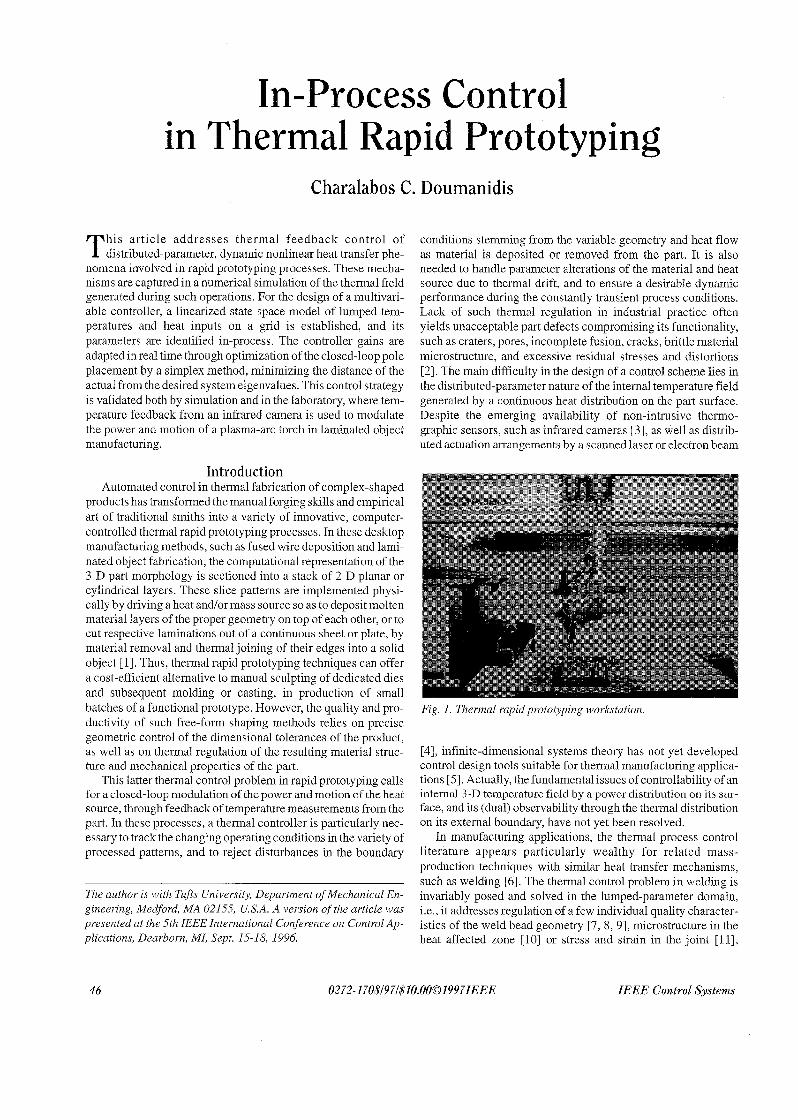
Fig. I . Thermal rapid prototyping workstation.

[4], infinite-dimensional systems theory has not yet developed control design tools suitable for thermal manufacturing applications [ 5 ] . Actually, the fundamental issues of controllability of an internal 3-D temperature field by a power distribution on its surface, and its (dual) observability through the thermal distribution on its external boundary, have not yet been resolved.

In manufacturing applications, the thermal process control literature appears particularly wealthy for related mass- production techniques with similar heat transfer mechanisms, such as welding [6]. The thermal control problem in welding is invariably posed and solved in the lumped-parameter domain, i.e., it addresses regulation of a few individual quality character- istics of the weld bead geometry [7, 8, 91, microstructure in the heat affected zone [lo] or stress and strain in the joint [11],

46 0272- 1708/97/$10.00O19971E E E IEEE Control Systems

through commensurate distinct welding conditions, such as torch power, speed, and wire feed. Several successful lumped controllers have been designed for a variety of welding methods, using artificial intelligence [ 121, neural network [ 131, expert system [14], or intelligent control algorithms [15]. A distributed- parameter approach to regulation of temperature fields has also been introduced for the new scan welding technique [ 161, as well as classical heat treatment [ 171. However, this formulation led to control tools of limited applicability, as the computational load of the controller [ 161 or the bandwidth requirements of the distributed sensor [ 171 would render the infinite-dimensional algorithms appropriate for off-line process scheduling only, and definitely prohibitive for real-time implementation on complex geometric patterns typical in rapid prototyping.

The objective of this article is to circumvent these limitations and develop a practical thermal control methodology for rapid prototyping techniques. Thus, a numerical distributed-parameter process description is reformulated as a finite-dimensional, MIMO relation of temperatures to heat inputs at the nodes of a grid spanning the part geometry, and a state space model linearized at the nominal process conditions is developed. This provides the basis for design of a multivariable control strategy, obtaining the desired closed-loop performance specifications by pole placement, which is optimized in-process by a simplex technique. The resulting adaptation of the controller is also based on real-time identification of the thermal process parameters by infrared temperature data. The computational efficiency of this algorithm allows for its laboratory implementation and testing on a plasma-arc thermal processing setup. Although experimental validation is provided for laminated object manufacturing operations, the methodology is intended for generic thermal rapid prototyping as well as conventional methods such as cutting, joining, and so on.

Molten Puddle

Coarse Mesh

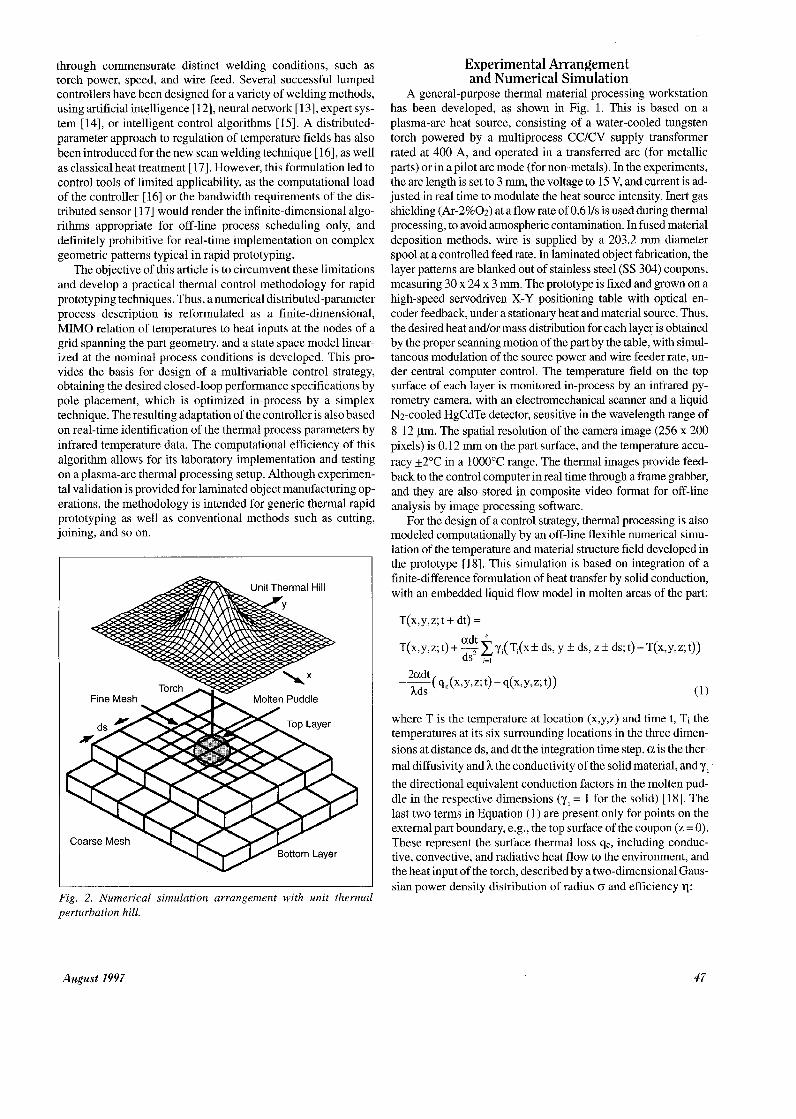
Fig. 2. Numerical simulation arrangement with unit thermal perturbation hill.

Experimental Arrangement and Numerical Simulation

A general-purpose thermal material processing workstation has been developed, as shown in Fig. 1. This is based on a plasma-arc heat source, consisting of a water-cooled tungsten torch powered by a multiprocess CC/CV supply transformer rated at 400 A, and operated in a transferred arc (for metallic parts) or in a pilot arc mode (for non-metals). In the experiments, the arc length is set to 3 mm, the voltage to 15 V, and current is ad- justed in real time to modulate the heat source intensity. Inert gas shielding (Ar-2%02) at a flow rate of 0.6 Vs is used during thermal processing, to avoid atmospheric contamination. In fused material deposition methods, wire is supplied by a 203.2 mm diameter spool at a controlled feed rate. In laminated object fabrication, the layer patterns are blanked out of stainless steel (SS 304) coupons, measuring 30 x 24 x 3 mm. The prototype is fixed and grown on a high-speed servodriven X-Y positioning table with optical en- coder feedback, under a stationary heat and material source. Thus, the desired heat and/or mass distribution for each layer is obtained by the proper scanning motion of the part by the table, with simultaneous modulation of the source power and wire feeder rate, under central computer control. The temperature field on the top surface of each layer is monitored in-process by an infrared py- rometry camera, with an electromechanical scanner and a liquid N2-cooled HgCdTe detector, sensitive in the wavelength range of 8-12 pm. The spatial resolution of the camera image (256 x 200 pixels) is 0.12 mm on the part surface, and the temperature accu- racy *2"C in a 1000°C range. The thermal images provide feedback to the control computer in real time through a frame grabber, and they are also stored in composite video format for off-line analysis by image processing software.

For the design of a control strategy, thermal processing is also modeled computationally by an off-line flexible numerical simulation of the temperature and material structure field developed in the prototype [18]. This simulation is based on integration of a finite-difference formulation of heat transfer by solid conduction, with an embedded liquid flow model in molten areas of the part:

T(x,y,z; t + dt) =

T(x,Y,z; t) + -E adt y,( T,(x+ ds, y f ds, z k ds; t) - T(x,~,z; t)) ds2 ,=,

where T is the temperature at location (x,y,z) and time t, Ti the temperatures at its six surrounding locations in the three dimensions at distance ds, and dt the integration time step. a is the thermal diffusivity and h the conductivity of the solid material, and y, the directional equivalent conduction factors in the molten puddle in the respective dimensions (y, = 1 for the solid) [ 181. The last two terms in Equation (1) are present only for points on the external part boundary, e.g., the top surface of the coupon (z = 0). These represent the surface thermal loss qe, including conduc- tive, convective, and radiative heat flow to the environment, and the heat input of the torch, described by a two-dimensional Gaus- sian power density distribution of radius 0 and efficiency q:

August 1997 47

'emDerature &

la

Ib

mm

2a.

I 2b.

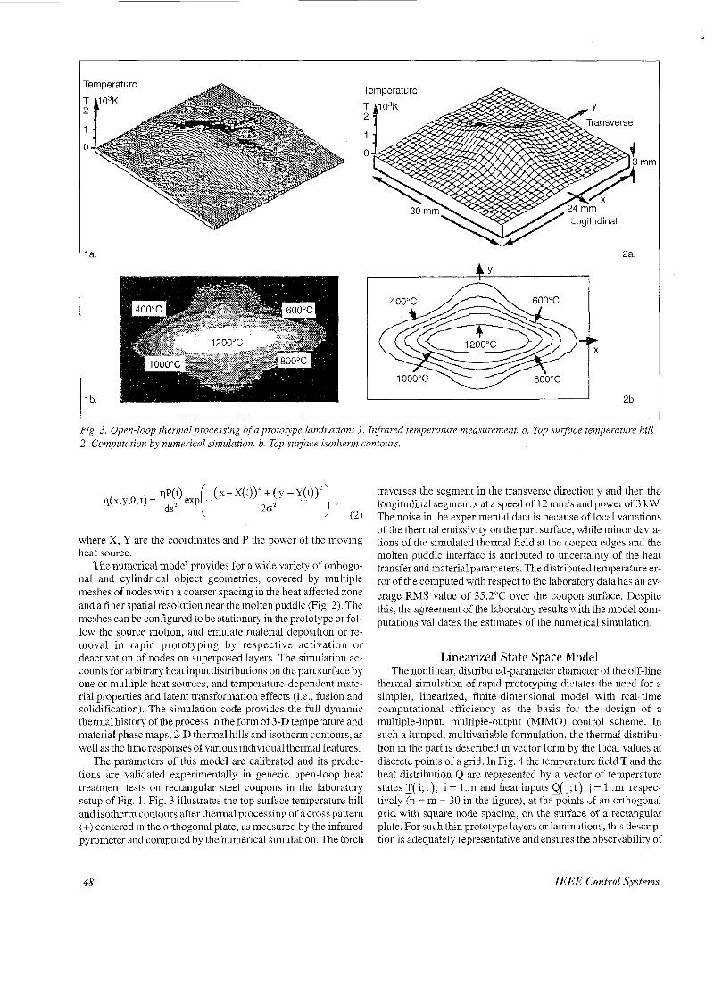
Fig. 3. Open-loop thermal processing of a prototype lamination: I . Infrared temperature measurement. a. Top su$ace temperature hill 2. Computation by numerical simulation. b. Top surface isotherm contours.

where X, Y are the coordinates and P the power of the moving heat source.

The numerical model provides for a wide variety of orthogonal and cylindrical object geometries, covered by multiple meshes of nodes with a coarser spacing in the heat affected zone and a finer spatial resolution near the molten puddle (Fig. 2). The meshes can be configured to be stationary in the prototype or fol- low the source motion. and emulate material deposition or removal in rapid prototyping by respective activation or deactivation of nodes on superposed layers. The simulation ac- counts for arbitrary heat input distributions on the part surface by one or multiple heat sources, and temperature-dependent material properties and latent transformation effects (i.e., fusion and solidification). The simulation code provides the full dynamic thermal history of the process in the form of 3-D temperature and material phase maps, 2-D thermal hills and isotherm contours, as well as the time responses of various individual thermal features.

The parameters of this model are calibrated and its predic- tions are validated experimentally in generic open-loop heat treatment tests on rectangular steel coupons in the laboratory setup of Fig. 1. Fig. 3 illustrates the top surface temperature hill and isotherm contours after thermal processing of a cross pattern (+) centered in the orthogonal plate, as measured by the infrared pyrometer and computed by the numerical simulation. The torch

traverses the segment in the transverse direction y and then the longitudinal segment x at a speed of 12 m d s and power of 3 kW. The noise in the experimental data is because of local variations of the thermal emissivity on the part surface, while minor deviations of the simulated thermal field at the coupon edges and the molten puddle interface is attributed to uncertainty of the heat transfer and material parameters. The distributed temperature er- ror of the computed with respect to the laboratory data has an average RMS value of 35.2"C over the coupon surface. Despite this, the agreement of the laboratory results with the model computations validates the estimates of the numerical simulation.

Linearized State Space Model The nonlinear, distributed-parameter character of the off-line

thermal simulation of rapid prototyping dictates the need for a simpler, linearized, finite-dimensional model with real-time computational efficiency as the basis for the design of a multiple-input, multiple-output (MIMO) control scheme. In such a lumped, multivariable formulation, the thermal distribution in the part is described in vector form by the local values at discrete points of a grid. In Fig. 4 the temperature field T and the heat distribution Q are represented by a vector of temperature statesT(i;t), i = l..n andheatinputsQ(j;t),i=l..m respectively (n = m = 30 in the figure), at thepoints uf an orthogonal grid with square node spacing, on the surface of a rectangular plate. For such thin prototype layers or laminations, this description is adequately representative and ensures the observability of

48 IEEE Control Systems

the internal thermal state in the part by surface output measurements through non-contact infrared thermometry. The grid ele- ment size Ds = 6mm is selected by compromise between spatial resolution and computational efficiency of the thermal formulation. Thus, this process model can be expressed in linearized, state space form in the neighborhood of some nominal thermal equilibrium as:

(3) - T(i;t) = A(i,h)'T(h;t)+ B(i,j)Q(j;t) -

where the temperature state vector T E R" and the heat input vector Q E Rm are measured relative to the nominal temperature set To generated at the standard operating conditions Qo, of thermal processing, typically defined by numerical simulation. The n x n state matrix A(i,h) and the nxm input matrix B(ij) describe the thermal process dynamics, and their elements express the thermal rate of change at point i because of a unit temperature T(h) at node h or a unit heat input QQ) at node j, respectively. These can

L tmm

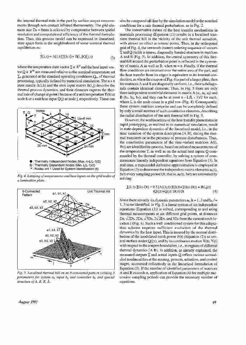
0 :Thermally Independent Nodes (Max. n-L(L-1)/2) @ :Thermally Dependent Nodes (Min. L(L-1)/2) * : Nodes wrt 1 Used for System Identification (6)

Fig. 4. Lumping of temperatures and heat inputs on the grid nodes of a lamination plate.

8-Connected Unit Thermal Hill Pattern

a i , b l , z h

Fig. 5. Localized thermal hill on an 8-connected pattern yielding 3 parameters for system ai, input bi, and controller ki, and special structure of A, B, K, b.

also be computed off-line by the simulation model at the nominal conditions for a unit thermal perturbation, as in Fig. 2.

The conservative nature of the heat transfer mechanisms in materials processing (Equation (1)) results in a localized transient thermal hill in the vicinity of the unit thermal actuation, with almost no effect at remote points. Thus, in the orthogonal grid of Fig. 4, the sawtooth (raster) ordering sequence of vectors T and Q yields a sparse, diagonally banded structure in matrices A and B (Fig. 5 ) . In addition, the central symmetry of this thermal hill around the perturbation point is reflected in the symmetry of matrix A as well as B, when m = n. Finally, if the thermal flow conditions are invariant over the entire area of the part, and the heat transfer from its edges is equivalent to its internal conduction, as when the coupon of Fig. 4 is part of a larger plate, then the matrices A and B are diagonally uniform, i.e., their subdiago- nals contain identical elements. Thus, in Fig. 5 there are only three independent nontrivial elements in matrix A (al, q, a3) and B (bi, b2, b3), and they can be at most n - L(L - 1)/2 for each, where L is the node count in a grid row (Fig. 4). Consequently, these system matrices comprise and can be completely defined by only a small number of such constitutive elements, describing the radial distribution of the unit thermal hill in Fig. 5.

However, the nonlinearities of the heat transfer phenomena in rapid prototyping, as realized in its numerical simulation, result in state-dependent dynamics of the linearized model, i.e., in the time variation of the system description [A B], during the thermal transients or in the presence of process disturbances. Thus, the constitutive parameters of the time-variant matrices A(t), B(t) are identified in-process, based on infrared measurements of the temperatures 1, as well as on the actual heat inputs Q com- manded by the thermal controller, by solving a system of commensurate linearly independent equations from Equation (3). In real time, a trapezoidal derivative approximation is employed in Equation (3) to determine the independent matrix elements ak(t), bi(t) every sampling period Dt, that is, ak(t), bl(t) are estimated by solving:

- T(i; t)-T(i;t-Dt) = 0.5 [A(i,h;t) (T(h;t)+T(h;t-Dt)) + B(ij;t) (Qci ;t)+Q(i;t-Dt))l Dt (4)

Since there are only six dynamic parameters ak, k = 1 ..3 and bl, 1 = 1 ..3 to be identified in Fig. 5, a linear system of six independent equations (Equation (3)) is solved, corresponding to and using thermal measurements at six different grid points, at distances Ds, A D S , 2Ds, ~ D s , 2&Ds, and 3Ds from the current torchlo- cation J (Fig. 4). Such a well-conditioned system for this adaptation scheme requires sufficient excitation of the thermal dynamics by the heat input. This is insured by the normal distribution of the modulated torch power P(t) (Equation ( 2 ) ) to several surface nodes QQ;t), and by its continuous motion X(t), Y(t) with respect to the coupon boundaries, i.e., to regions of different thermal dynamics [A B]. In addition, as already explained, the measured outputs and actual inputs Q reflect various unmod- eled nonlinearities at the sensing, process, actuation, and control stages, accounted collectively in the linearized formulation of Equation (3). If the number of identified parameters of matrices A and B exceeds n, application of Equation (4) for multiple successive sampling periods can provide the necessary number of equations.

August 1997 49

Pole Placement of MIMO Controller The state space model of Equation (3) is suitable for the de-

sign of a multivariable thermal control strategy, where the desired dynamics of the closed-loop system are stipulated by proper placement of its poles. Thus, the MIMO control law em- ploys in-process sensing and feedback of the thermal states 1: to determine the heat inputs Q as follows:

Qci;t) = K(i,h)T(h;t), (5)

and by substituting in Equation (3):

- T(i; t) = [A(i,h) + B(i, j)K(j, h)]T(h; t) = i ( i , h)T(h; t) , (6)

where K is the mxn matrix of control gains and A = A + BK the n x n state matrix of the closed-loop system. If the open-loop thermal system is completely controllable, i.e., the controllability matrix is of full rank n, then the gains in matrix K can be determined to place the eigenvalues pl, i = 1 ..n of matrix A (the poles of the feedback system) exactly to the specified values pl* [ 191. These desired poles, which decide the dynamic performance of the regulated process, should be selected so as to ensure metal- lurgically favorable thermal cycles in the part, yielding a desirable material structure and the resulting mechanical properties of the prototype.

However, since controllability of the finite-dimensional model of thermal processing is not guaranteed by distributed- parameter systems theory, pole placement cannot be obtained by standard algorithms [20]. In addition, these methods require that all elements in matrix K be variable and subject to unconstrained determination. In practice, though, it is desirable to simplify the controller implementation by eliminating (setting to 0) certain gains of K corresponding to inefficient input-output connec- tions. Such constrained feedback control is also advantageous in the thermal operation of Fig. 5. Here the localized temperature hill generated by a concentrated heat input Q(i;t) at point j sug- gests that this should be determined only by the temperatures T(h;t) at a few surrounding points h, for example on an 8- connected pattern around the center j, with no effect from remote temperatures. The central symmetry of this thermal field also dictates that the value Q(i;t) be contributed by the temperatures T(h;t), weighted by gains k corresponding to the radial distance of each point h from the center j. Thus only three independent gains kl, k2, and k3 are needed for all points of this symmetric pattern, lying at three different radii from j. The control law of Equation (5) is therefore simplified to:

+k3 [T(i-L- 1 ;t)+lCCj -L+ 1 ;t)+TCj +L- 1 ;t)+TQ+L+ 1 ;t)]. (7) For points j on the external grid boundary, the temperatures of points h falling outside the grid are replaced by those of the antid- iametric internal points with respect to the centerj. This selection of gains yields also a sparse, uniform diagonally banded strnc- ture in matrix K, similar to that of the open-loop system matrices (Fig. 5). As a consequence, the control law of Equation (7) pre- serves the symmetry of the closed-loop state matrix A, which also has a structure similar to that of Fig. 5.

Since for this constrained feedback scheme an exact placement of the eigenvalues of matrix A may not be possible, an alter-

50

Complex Plane Im 4

I I D= R M S (d i)

I

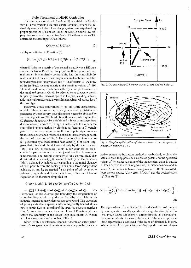
Fig. 6. Distance index D between actual pi and desired poles p*.

I Y

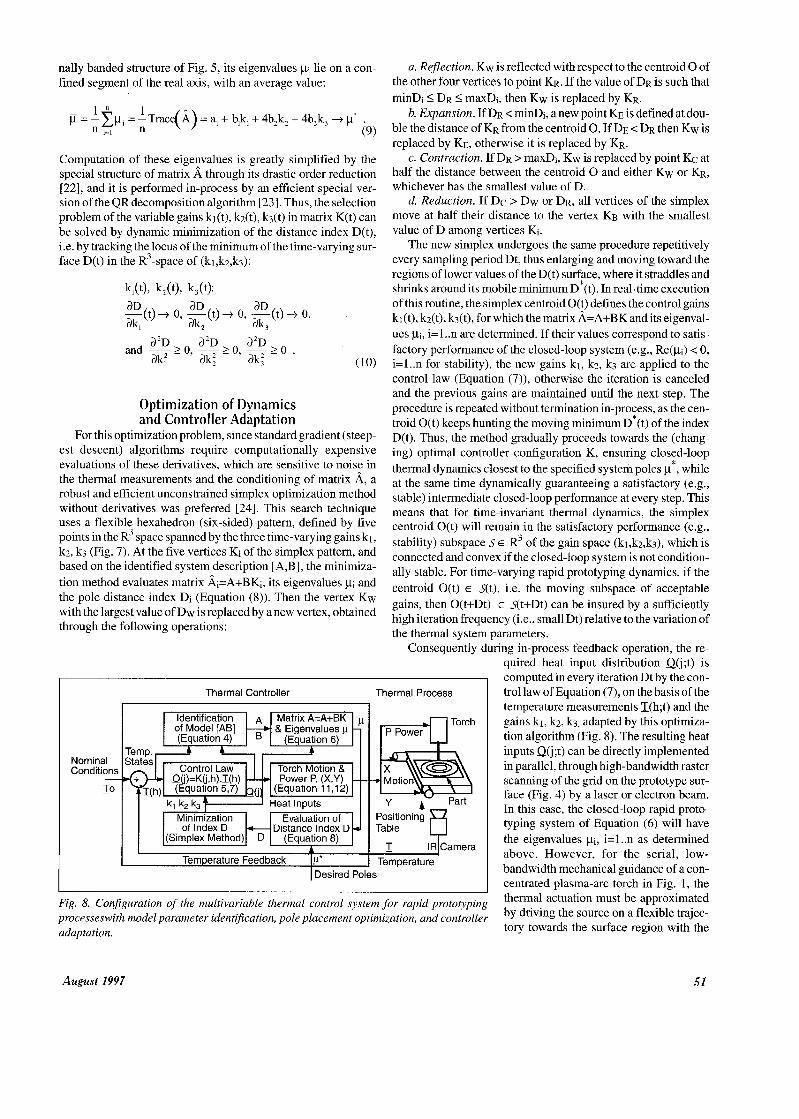
Fig. 7. Simplex optimization of distance index D in the space of controller gains kl , k2, k3.

native general optimization method is established, to place the actual closed-loop poles mi as close as possible to the specified values pi* by proper selection of the independent gains in matrix K. For a current selection of gains K(t), a Euclidean norm of distance D(t) is defined between the eigenvalues /Li(t) of the closed- loop system matrix A(t) = A(t)+B(t) K(t) and the desired poles pi* (Fig. 6) [21]:

(8)

The eigenvalues pi* are dictated by the desired thermal process dynamics, and are usually specified at a single location pi = p = -3/ts, i=l..n where ts is the 95% settling time of the desired temperature transients. An exact placement of the system poles to these eigenvalues is achieved if the value of distance D is zero. When matrix A is symmetric and displays the uniform, diago-

* *

IEEE Control Systems

nally banded structure of Fig. 5 , its eigenvalues k 1' ie on a con- fined segment of the real axis, with an average value:

1 " 1 = - z p , = -Trace(i) = a, + b,k, + 4b,k, + 4b,k, -+ p* .

(9) n ,=I n

Computation of these eigenvalues is greatly simplified by the special structure of matrix A through its drastic order reduction [22], and it is performed in-process by an efficient special version of the QR decomposition algorithm [23]. Thus, the selection problem of the variable gains kl(t), kz(t), k3(t) in matrix K(t) can be solved by dynamic minimization of the distance index D(t), i.e. by tracking the locus of the minimum of the time-varying surface D(t) in the R3-space of (ki,kz,k3):

k,(t), k*(t), kdt):

Optimization of Dynamics and Controller Adaptation

For this optimization problem, since standard gradient (steep- est descent) algorithms require computationally expensive evaluations of these derivatives, which are sensitive to noise in the thermal measurements and the conditioning of matrix A, a robust and efficient unconstrained simplex optimization method without derivatives was preferred [24]. This search technique uses a flexible hexahedron (six-sided) pattern, defined by five points in the R3 space spanned by the three time-varying gains kl, kz, k3 (Fig. 7). At the five vertices Ki of the simplex pattern, and based on the identified system description [A,B], the minimization method evaluates matrix Ai=A+BKi, its eigenvalues pi and the pole distance index Di (Equation (8)). Then the vertex Kw with the largest value of Dw is replaced by a new vertex, obtained through the following operations:

a. Reflection. Kw is reflected with respect to the centroid 0 of the other four vertices to point KR. If the value of DR is such that minDl 5 DR 5 maxD,, then KW is replaced by KR.

b. Expansion. If DR < minDi, a new point KE is defined at dou- ble the distance of KR from the centroid 0. If DE < DR then Kw is replaced by KE, otherwise it is replaced by KR.

c. Contraction. If DR > maxD,, KW is replaced by point Kc at half the distance between the centroid 0 and either Kw or KR, whichever has the smallest value of D.

d. Reduction. If Dc > Dw or DR, all vertices of the simplex move at half their distance to the vertex KB with the smallest value of D among vertices Kl.

The new simplex undergoes the same procedure repetitively every sampling period Dt, thus enlarging and moving toward the regions of lower values of the D(t) surtace, where it straddles and shrinks around its mobile minimum D (t). In real-time execution of this routine, the simplex centroid O(t) defines the control gains ki(t), k2(t), k3(t), for which the matrix A=A+BK and its eigenvalues pl, i=l..n are determined. If their values correspond to satisfactory performance of the closed-loop system (e.g., Re(pi) < 0, i=l..n for stability), the new gains kl, k2, k3 are applied to the control law (Equation (7)), otherwise the iteration is canceled and the previous gains are maintained until the next step. The procedure is repeated without termination in-process, as the centroid O(t) keeps hunting the moving minimum D*(t) of the index D(t). Thus, the method gradually proceeds towards the (changing) optimal controller configuration K, ensuring closed-loop thermal dynamics closest to the specified system poles p*, while at the same time dynamically guaranteeing a satisfactory (e.g., stable) intermediate closed-loop performance at every step. This means that for time-invariant thermal dynamics, the simplex centroid O(t) will remain in the satisfactory performance (e.g., stability) subspace SE R3 of the gain space (kl,kz,k3), which is connected and convex if the closed-loop system is not condition- ally stable. For time-varying rapid prototyping dynamics, if the centroid O(t) E S(t), i.e. the moving subspace of acceptable gains, then O(t+Dt) E S(t+Dt) can be insured by a sufficiently high iteration frequency (i.e., small Dt) relative to the variation of the thermal system parameters.

Consequently during in-process feedback operation, the re-

Thermal Controller Thermal Process I I

Identification A Matrix A=A+BK of Model [AB] - & Eigenvalues p - (Equation 4) (Equation 6)

Torch Motion &

Minimization Evaluation of of Index D

(Simplex Method) D (Equation 8)

Temperature Feedback lP*

+- Distance Index D +

A

I Desired Poles

Torch

I

Table

Temperature

Fig. 8. Conjiguration of the multivariable thermal control system for rapid prototyping processeswith model parameter identijication, pole placement optimization, and controller adaptation.

quired heat input distribution Q(j;t) is computed in every iteration Dt by the control law of Equation (7), on the basis of the temperature measurements T(h;t) and the gains kl, k2, k3, adapted by this optimization algorithm (Fig. 8). The resulting heat inputs Q(j;t) can be directly implemented in parallel, through high-bandwidth raster scanning of the grid on the prototype surface (Fig. 4) by a laser or electron beam. In this case, the closed-loop rapid prototyping system of Equation (6) will have the eigenvalues pi, i=l..n as determined above. However, for the serial, low- bandwidth mechanical guidance of a concentrated plasma-arc torch in Fig. 1, the thermal actuation must be approximated by driving the source on a flexible trajectory towards the surface region with the

August 1997 51

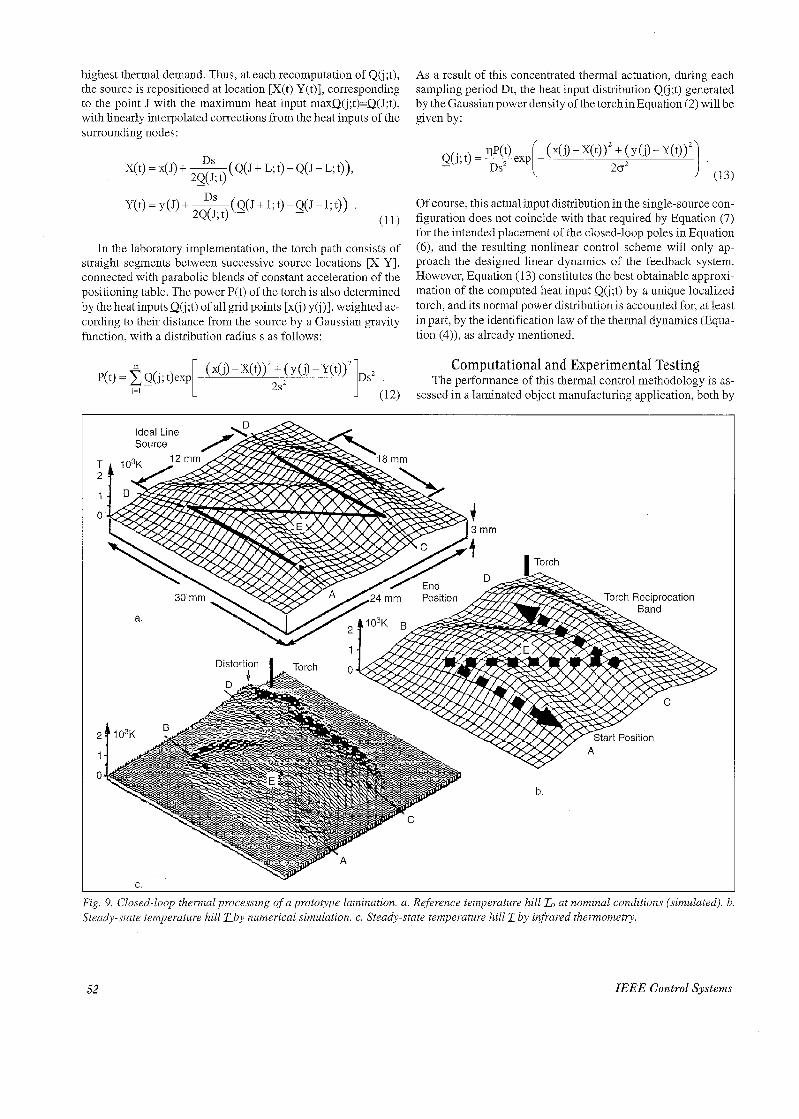
highest thermal demand. Thus, at each recomputation of Q(j;t), the source is repositioned at location [X(t) Y(t)], corresponding to the point J with the maximum heat input maxQ(j;t)=Q(J;t), with linearly interpolated corrections from the heat inputs of the surrounding nodes:

Ds X(t) = x( J) + ~ (Q(J + L; t) - Q(J - L; t)), - 2QJ; t)

In the laboratory implementation, the torch path consists of straight segments between successive source locations [X Y], connected with parabolic blends of constant acceleration of the positioning table. The power P(t) of the torch is also determined by the heat inputs Q(j;t) of all grid points [xu) y(j)], weighted ac- cording to their distance from the source by a Gaussian gravity function, with a distribution radius s as follows:

As a result of this concentrated thermal actuation, during each sampling period Dt, the heat input distribution Q(j;t) generated by the Gaussian power density of the torch in Equation (2) will be given by:

Of course, this actual input distribution in the single-source configuration does not coincide with that required by Equation (7) for the intended placement of the closed-loop poles in Equation (6), and the resulting nonlinear control scheme will only approach the designed linear dynamics of the feedback system. However, Equation (13) constitutes the best obtainable approximation of the computed heat input Q(j;t) by a unique localized torch, and its normal power distribution is accounted for, at least in part, by the identification law of the thermal dynamics (Equa- tion (4)), as already mentioned.

Computational and Experimental Testing The performance of this thermal control methodology is as-

sessed in a laminated object manufacturing application, both by

c.

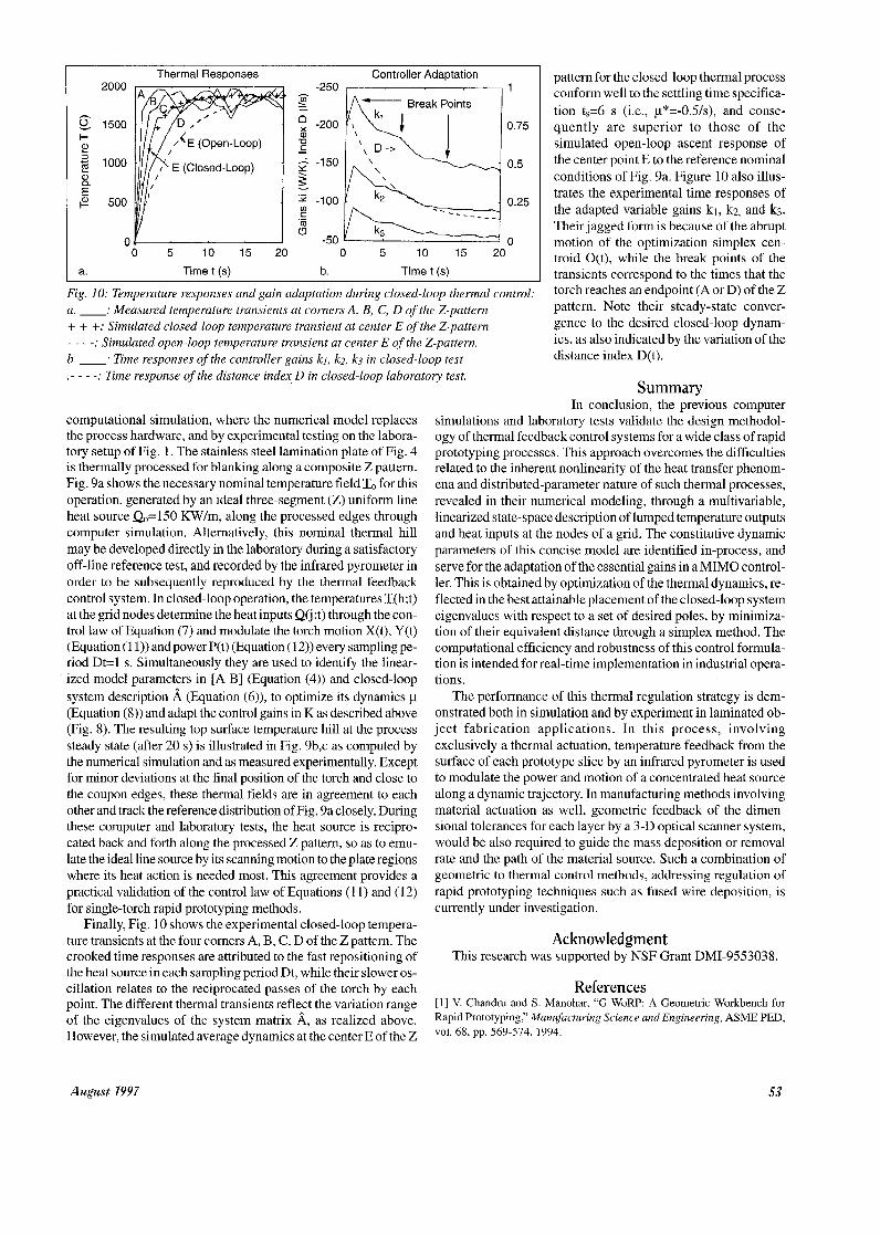
Fig. 9. Closed-loop thermal processing of a prototype lamination. a. Reference temperature hill To at nominal conditions (simulated). b. Steady-state temperature hill T b y numerical simulation. c. Steady-state temperature hill 1 by infrared thermometry.


2000

1500 I- 2 9

E $?? 500

2 1000

d

n

I n- Break Points

Thermal Responses

L “0 5 10 15 20

a. Timet (s)

-200

-1 50

-100

-50

0.75

0.5 ‘ 0.25

n

- - - - _ _

0 5 10 15 20-

b. Timet (s)

Fig. 10: Temperature responses and gain adaptation during closed-loop thermal control: a. -: Measured temperature transients at corners A, B, C, D of the Z-pattern + + +: Simulated closed-loop temperature transient at center E of the Z-pattern - - - -: Simulated open-loop temperature transient at center E of the Z-pattern. b. -: Time responses of the controller gains k l , k2, k3 in closed-loop test .- - - -: Time response of the distance index D in closed-loop laboratory test.

computational simulation, where the numerical model replaces the process hardware, and by experimental testing on the laboratory setup of Fig. 1. The stainless steel lamination plate of Fig. 4 is thermally processed for blanking along a composite Z pattern. Fig. 9a shows the necessary nominal temperature field To for this operation, generated by an ideal three-segment (Z) uniform line heat source Q,=l50 KW/m, along the processed edges through computer simulation. Alternatively, this nominal thermal hill may be developed directly in the laboratory during a satisfactory off-line reference test, and recorded by the infrared pyrometer in order to be subsequently reproduced by the thermal feedback control system. In closed-loop operation, the temperatures T(h;t) at the grid nodes determine the heat inputs Q(j;t) through the control law of Equation (7) and modulate the torch motion X(t), Y(t) (Equation (1 1)) and power P(t) (Equation (1 2) ) every sampling period Dt=l s. Simultaneously they are used to identify the linearized model parameters in [A B] (Equation (4)) and closed-loop system description (Equation (6)), to optimize its dynamics p (Equation (8)) and adapt the control gains in K as described above (Fig. 8). The resulting top surface temperature hill at the process steady state (after 20 s) is illustrated in Fig. 9b,c as computed by the numerical simulation and as measured experimentally. Except for minor deviations at the final position of the torch and close to the coupon edges, these thermal fields are in agreement to each other and track the reference distribution of Fig. 9a closely. During these computer and laboratory tests, the heat source is reciprocated back and forth along the processed Z pattern, so as to emulate the ideal line source by its scanning motion to the plate regions where its heat action is needed most. This agreement provides a practical validation of the control law of Equations (1 1) and (1 2) for single-torch rapid prototyping methods.

Finally, Fig. 10 shows the experimental closed-loop temperature transients at the four corners A, E, C, D of the Z pattern. The crooked time responses are attributed to the fast repositioning of the heat source in each sampling period Dt, while their slower os- cillation relates to the reciprocated passes of the torch by each point. The different thermal transients reflect the variation range of the eigenvalues of the system matrix A, as realized above. However, the simulated average dynamics at the center E of the Z

pattern for the closed-loop thermal process conform well to the settling time specifica- tion ts=6 s (i.e., p*=-OS/s), and consequently are superior to those of the simulated open-loop ascent response of the center point E to the reference nominal conditions of Fig. 9a. Figure 10 also illustrates the experimental time responses of the adapted variable gains kl, kz, and k3. Their jagged form is because of the abrupt motion of the optimization simplex centroid O(t), while the break points of the transients correspond to the times that the torch reaches an endpoint (A or D) of the Z pattern. Note their steady-state conver- gence to the desired closed-loop dynamics, as also indicated by the variation of the distance index D(t).

Summary In conclusion, the previous computer

simulations and laboratory tests validate the design methodology of thermal feedback control systems for a wide class of rapid prototyping processes. This approach overcomes the difficulties related to the inherent nonlinearity of the heat transfer phenomena and distributed-parameter nature of such thermal processes, revealed in their numerical modeling, through a multivariable, linearized state-space description of lumped temperature outputs and heat inputs at the nodes of a grid. The constitutive dynamic parameters of this concise model are identified in-process, and serve for the adaptation of the essential gains in a MIMO controller. This is obtained by optimization of the thermal dynamics, reflected in the best attainable placement of the closed-loop system eigenvalues with respect to a set of desired poles, by minimization of their equivalent distance through a simplex method. The computational efficiency and robustness of this control formulation is intended for real-time implementation in industrial operations.

The performance of this thermal regulation strategy is dem- onstrated both in simulation and by experiment in laminated object fabrication applications. In this process, involving exclusively a thermal actuation, temperature feedback from the surface of each prototype slice by an infrared pyrometer is used to modulate the power and motion of a concentrated heat source along a dynamic trajectory. In manufacturing methods involving material actuation as well, geometric feedback of the dimensional tolerances for each layer by a 3-D optical scanner system, would be also required to guide the mass deposition or removal rate and the path of the material source. Such a combination of geometric to thermal control methods, addressing regulation of rapid prototyping techniques such as fused wire deposition, is currently under investigation.

Acknowledgment This research was supported by NSF Grant DMI-9553038.

References [l] V. Chandru and S . Manohar, “G-WoRP: A Geometric Workbench for Rapid Prototyping,” Manufacturing Science and Engineering, ASME PED, vol. 68, pp. 569-574, 1994.

August 1997 53

121 EA. McClintock and A.S. Argon, “Mechanical Behavior of Materials,” Addison-Wesley, Reading, MA, 1966.

[3] W.E. Lukens and R.A. Morris, “Infrared Temperature Sensing of Cooling Rates for Arc Welding Control,” Welding Journal, pp. 27-39, June 1982.

[4] W.M. Steen, “Laser Material Processing,” Springer-Verlag, London, U.K., 1991.

[SI S.G. Tzafestas, “Distributed Parameter Control Systems,” Pergamon Press, Oxford, 1982.

[6] D.A. Dornfeld, M. Tomizuka, and G. Langari, “Modelling and Adaptive Control of Arc Welding,” Measurement & Control for Batch Manufacturing, pp. 53-64, November 1982.

[7] M. Hale, “Multivariable Geometry Control of GMA Welding,” Ph.D Thesis, Dept. of Mechanical Engineering, MIT, Cambridge MA, 1988.

[8] A. Suzuki, D.E. Hardt and L. Valavani, “Application of Adaptive Control Theory to On-Line GTA Weld Geometry Regulation,” ASME Journal of Dynamic Systems, Measurement and Control, vol. 113, no. 1, pp. 93.103, 1989.

[9] R.A. Masmoudi and D.E. Hardt, “Multivariable Control of Geometric and Thermal Properties in GMAW,” Trends in Welding Research, ASM Intl, Gatlinburg, TN, 1992.

[lo] C.C. Doumanidis and D.E. Hardt, “Simultaneous In-Process Control of Heta Affected Zone and Cooling Rate,” Welding Journal, vol. 69/5, pp. 186s-l96s, 1990.

[I 11 H. Miyachi, “In-Process Control of Root-Gap Changes During Butt Welding,” Ph.D. Thesis, Dept. of Mechanical Engineering, MIT, Cambridge MA, 1989.

[12] H.S. Cho, “Application of AI to Welding Process Automation,” ASME Ja- padUSA Symposium on Flexible Automation, Kobe, Japan, pp. 303-308,1992.

[13] K. Andersen, G.E. Cook and R.J. Barnett, “Gas Tungsten Arc Welding Process Control Using Artificial Neural Networks,” Trends in Welding Re- search, ASM, pp. 877-881, 1992.

[ 141 E Misra, “Expert System for GMA Welding of Aluminum,” International Trends in Welding Science and Technology, ASM Intl., pp. 949-956, 1993.

[15] H.B. S m m , “Intelligent Sensing and Control of Arc Weldmg,” Interruz- tionalTrends in WeldingScienceand Technology, ASMIntl.,pp. 843-851,1993.

[16] C.C. Doumanidis, “Modeling and Control of Timeshared and Scanned Torch Welding,” ASME J. ofDyn. Systems Measurement & Control, Vol. 116 No. 3, pp. 387-395, 1994.

[ 171 C.C. Doumanidis, “Heat Treatment Control by Polytope Methods,” Proc. ofthe 1995 American Control Conference, v. 2, Seattle, WA, pp. 1275- 1279, June 1995.

[18] B.P. Marquis and C.C. Doumanidis, “Distributed-Parameter Simulation of the Scan Welding Process,” ZASTED Con$ on Model. & Simulation, Pitts- burgh, PA, pp. 146-149, 1993.

[ 191 T. Kailath, Linear Systems, Prentice-Hall, Englewood Cliffs, NJ, 1980.

[20] R.W. Bass and 1. Gura, “High Order Design via State-Space Considera- tions,” Proceedings of the 1965 Joint Automatic Control Conference, Troy, NY, pp. 311-318, 1965.

[21] C.C. Doumanidis, “Numerical Techniques for Designing Output Feed- back and Robust Controllers,” M.S. Thesis, Dept. of Mech. Eng., Northwest- ern Univ., Evanston, IL, 1985.

[22] J.R. Bunch and D.J. Rose, Sparse Matrix Computations, Academic Press, NY, 1976.

[23] J.G.F. Francis, “The QR Transformation I, 11,” Computer Journal 4, pp. 69-79, 1961.

[24] J.A. Nelder and R. Mead, “A Simplex Method for Function Minimiza- tion,” Computer Journal 7, pp. 24-31, 1964.

Charalabos Doumanidis, associate professor of Mechanical Engineering at Tufts University, holds his Ph.D. from MIT (1988), his M.S. fromNorthwest- em University (1985) and his Diploma from the Aristotelian University of Thessaloniki (1983). His research focuses on manufacturing processes including thermal rapid prototyping and welding, systems modeling and adaptive control, robotics and automation, and biomedical engineering. He has authored over 90 papers in joumals and conferences, serves as Associate Edi- tor for the International Journal of Modelling and Simulation, and has been the recipient of several awards, including the Presidential Faculty Fellow award from the White House in 1995.


Documents

In-process control in thermal rapid prototyping