Journal of Methods and Measurement in the Social Sciences, Vol. 8, No. 2, 72-99, 2017

72

In Social Network Analysis, Which Centrality Index Should I Use?: Theoretical Differences and Empirical

Similarities among Top Centralities

Dawn Iacobucci Vanderbilt University

Rebecca McBride Deloitte

Deidre L. Popovich

Texas Tech University Maria Rouziou

Wilfrid Laurier University Ontario, CA, This research examines four frequently used centrality indices—degree, closeness, betweenness, and eigenvectors—to understand the extent to which their clear theoretical distinctions are reflected in differences in empirical performance. Even for stylized networks in which one centrality index may seem more relevant than the others, the four indices are frequently highly correlated. This result can be interpreted as good news: it does not diminish the conceptual distinctions, yet it suggests the indices are rather robust, yielding similar information about actors’ positions in networks, which can be reassuring given their widespread use by applied network analysts who may not appreciate the theoretically distinct origins and definitions. This research also compares computational speed across the centrality indices as another practical element that may help determine the choice of centrality index. Keywords: centrality; degree; closeness; betweenness; eigenvector centrality; social networks

Social networks and an interest in understanding social connections seem pervasive. In many social network studies, the starting point of the analysis is the identification of actors with disproportionately high or low social capital. Locating actors who are important in some manner is usually achieved via centrality indices. Numerous actor-level indices of centrality are available to characterize actors’ positions and structural ties in social networks. Freeman’s (1978) seminal paper introduced the distinct theoretical underpinnings for degree, closeness, and betweenness centralities. Degree reflects overall volumes of ties, closeness captures the extent to which the relational ties traverse few “degrees of separation,” and betweenness highlights those actors through whom much of the rest of the network is interconnected. In addition to these centrality measures, scholars have developed many more indices, each with its own character and strengths.

These centrality indices have been used in a wide variety of social network applications. Consider the following:

IACOBUCCI

73

Degree centralities are perhaps the easiest to understand—they reflect sheer numbers of links and/or the strengths of those ties. For example, certain social status is conveyed upon people who have many followers on Twitter (Zhang et al., 2015), or many friends or likes on Facebook (Sabate, Berbegal-Mirabent, Canabate, & Lebherz, 2014).

Actors with high closeness centralities are those who are directly interconnected to many other players in the network. The numerous direct ties can lend an efficiency in coordinating work efforts in alliances between organizations (e.g., Koschmann & Wanberg, 2016). Similarly, closeness can enhance the ability of animal groups who live together and are aided in achieving their group goals by their close interactions (Wey, Blumstein, Shen, & Jordan, 2008). As another example, people tend to pre-program phone numbers of their closest ties into their mobile phones; a simple observation being adopted by law enforcement agencies to locate criminals (Ferrara, De Meo, Catanese, & Fiumara, 2014). Closeness is also examined in brain connectivity data where local pathways affect overall circuitry (Rubinov & Sporns, 2010).

Betweenness has long been recognized as a quality that can enhance the social capital of employees in organizations who bridge departments because such boundary spanners influence the flow of communication and information between work groups (Brass, 1984). The importance of an actor with a high betweenness centrality can also be seen in the hub-and-spoke design of today’s airline industry. For example, when bad weather disrupts an airport that is a hub between other cities, customers are affected in the origin and destination cities (O’Kelly, 2016).

Experienced network scholars might appreciate the distinct relative advantages of different centrality indices in different network applications. Yet the vastness of the options of these (and other) centrality indices can make the choice overwhelming for scholars and practitioners with less network experience—an occurrence more frequent than ever given the increased popularity and study of social network phenomena. Thus, in this investigation, we examine four of the more frequently implemented centrality indices to ascertain whether their purported theoretical distinctions hold empirically. If not, could the selection of a theoretically suboptimal index disguise apparent structure or otherwise yield misleading results? If the indices perform differently on different structures of social networks, we would need to understand how to diagnose the identifying characteristics of a network to suggest the optimal selection of a centrality index. If instead, the indices are fairly similar in their empirical performance (even granting their conceptual differences),

CENTRALITY INDICES

74

then the selection of a centrality index is less critical and the values obtained are therefore more robust conceptually.

This research is intended to be useful in helping social network analysts select among the myriad of centrality indices. While network scholars emphasize theoretical distinctions, in practice it is not unusual for social network researchers to observe that their centralities are at least moderately correlated. To the best of our knowledge, these patterns have not been systematically examined, thus we seek to do so in this research. In addition, we conduct a complementary investigation into the relative computing times for the four centrality indices. The reasoning here is that if the empirical performances of the centrality indices are comparable, then the efficiencies with which the centralities may be estimated may become an important choice criterion, at least when analyzing large networks.

In the section that follows, we first draw on the literature and review the centrality indices that serve as the focus of this research. In Study 1, we examine the performance of the centrality indices on small, stylized network structures to observe the extent to which the different indices begin to capture unique network patterns. In Study 2, we extend the size of the exemplar networks, and Study 3 turns to the practical matter of the comparative computing times for the centralities as an indicator of the efficiencies of the algorithms. Literature and Definitions of Four Focal Centrality Indices

Novice social network analysts often find it difficult to discern which centrality index is most appropriate to use given their research data. The social network researcher has gone through what can often be substantial efforts to obtain a sociomatrix. Next, the researcher is eager to analyze the data to learn what patterns and structures are exhibited in the network. With data in hand, the network analyst opens any of a number of popular network analysis computing packages and finds vast numbers of choices of a centrality index to describe the network. We have empathy particularly for novice social network researchers for whom the numerous options can seem overwhelming. Their confusions leads to the inevitable question, “Which centrality index should I use?” The purpose of this research is to help assist in answering that question. Table 1 lists several popular social network analysis packages, beginning with UCINet (given both its prevalence and its importance in the legacy of social network analysis). These software providers offer users a substantial number of options. Yet there are only four centrality indices that appear across most of the software packages: degree, closeness, betweenness, and eigenvectors. Various research articles have certainly also considered alternative centrality indices, such as information

IACOBUCCI

75

centrality (Rothenberg et al., 1995; Stephenson & Zelen, 1989), or generalizations of indices for directed graphs (e.g., Freeman, Borgatti, Table 1 Centrality Indices Offered in Popular Social Network Analysis Packages and Procedures

Centralities

Package: d

egre

e

clo

sen

ess

bet

wee

nn

ess ei

gen

vec

tor

Other centrality indices:

UCINet attribute weighted, beta reach, Bonacich power, edge betweenness, flow betweenness, Hubbel, influence, information, inverse weighted degree, Katz

Mathematica eccentricity, edge betweenness, geoprojection, hub authority or HITS (hyperlink-induced topic search), Katz, link rank, PageRank, radiality, status

NetMiner community, coreness, decay, effects, HITS, information, flow betweenness, load, PageRank, power, status

NetworkX and LibSNA

current flow, communicability, dispersion, edge betweenness, Katz, load

NodeXL and SNAP

PageRank

Pajek Hubs-authorities, proximity prestige, Laplacian

StatNet Bonacich power, prestige, stress

& White, 1991; White & Borgatti 1994), weighted ties (e.g., Opsahl, Agneessens, & Skvoretz, 2002), graphs with inherent subgroup structures (e.g., Everett & Borgatti 1999), a focus on a micro (“local”) or macro (“global”) structure, or analyzing a particular actor through an egocentric network lens versus examining a collection of actors in a sociocentric approach to the network (cf., Scott, 2012). Yet for all the variety, the four indices we have selected—degree, closeness, betweenness, and eigenvectors—seem most transferable in their general use across network textbooks, research articles, and available software packages. Thus we focus on these four indices.

CENTRALITY INDICES

76

As Freeman (1978, p.219) stated, “…each [centrality] measure is associated with some sort of intuitive basis or rationale for its own particular structural property.” Here we consider those rationales and the computational formulae for each of the indices.

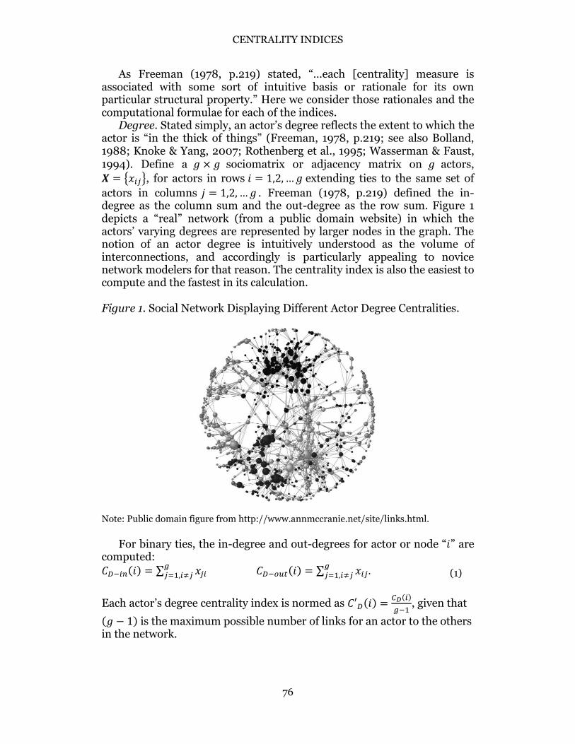
Degree. Stated simply, an actor’s degree reflects the extent to which the actor is “in the thick of things” (Freeman, 1978, p.219; see also Bolland, 1988; Knoke & Yang, 2007; Rothenberg et al., 1995; Wasserman & Faust, 1994). Define a 𝑔 × 𝑔 sociomatrix or adjacency matrix on 𝑔 actors,

𝑿 = {𝑥𝑖𝑗}, for actors in rows 𝑖 = 1,2, …𝑔 extending ties to the same set of

actors in columns 𝑗 = 1,2, …𝑔 . Freeman (1978, p.219) defined the in-degree as the column sum and the out-degree as the row sum. Figure 1 depicts a “real” network (from a public domain website) in which the actors’ varying degrees are represented by larger nodes in the graph. The notion of an actor degree is intuitively understood as the volume of interconnections, and accordingly is particularly appealing to novice network modelers for that reason. The centrality index is also the easiest to compute and the fastest in its calculation. Figure 1. Social Network Displaying Different Actor Degree Centralities.

Note: Public domain figure from http://www.annmccranie.net/site/links.html.

For binary ties, the in-degree and out-degrees for actor or node “𝑖” are

computed:

𝐶𝐷−𝑖𝑛(𝑖) = ∑ 𝑥𝑗𝑖𝑔𝑗=1,𝑖≠𝑗 𝐶𝐷−𝑜𝑢𝑡(𝑖) = ∑ 𝑥𝑖𝑗

𝑔𝑗=1,𝑖≠𝑗 .

Each actor’s degree centrality index is normed as 𝐶′𝐷(𝑖) =𝐶𝐷(𝑖)

𝑔−1, given that

(𝑔 − 1) is the maximum possible number of links for an actor to the others in the network.

(1)

IACOBUCCI

77

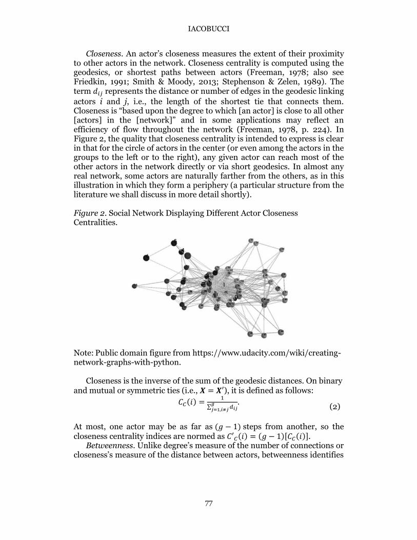
Closeness. An actor’s closeness measures the extent of their proximity to other actors in the network. Closeness centrality is computed using the geodesics, or shortest paths between actors (Freeman, 1978; also see Friedkin, 1991; Smith & Moody, 2013; Stephenson & Zelen, 1989). The term 𝑑𝑖𝑗 represents the distance or number of edges in the geodesic linking

actors i and j, i.e., the length of the shortest tie that connects them. Closeness is “based upon the degree to which [an actor] is close to all other [actors] in the [network]” and in some applications may reflect an efficiency of flow throughout the network (Freeman, 1978, p. 224). In Figure 2, the quality that closeness centrality is intended to express is clear in that for the circle of actors in the center (or even among the actors in the groups to the left or to the right), any given actor can reach most of the other actors in the network directly or via short geodesics. In almost any real network, some actors are naturally farther from the others, as in this illustration in which they form a periphery (a particular structure from the literature we shall discuss in more detail shortly). Figure 2. Social Network Displaying Different Actor Closeness Centralities.

Note: Public domain figure from https://www.udacity.com/wiki/creating-network-graphs-with-python.

Closeness is the inverse of the sum of the geodesic distances. On binary and mutual or symmetric ties (i.e., 𝑿 = 𝑿′), it is defined as follows:

𝐶𝐶(𝑖) =1

∑ 𝑑𝑖𝑗𝑔𝑗=1,𝑖≠𝑗

.

At most, one actor may be as far as (𝑔 − 1) steps from another, so the closeness centrality indices are normed as 𝐶′𝐶(𝑖) = (𝑔 − 1)[𝐶𝐶(𝑖)].

Betweenness. Unlike degree’s measure of the number of connections or closeness’s measure of the distance between actors, betweenness identifies

(2)

CENTRALITY INDICES

78

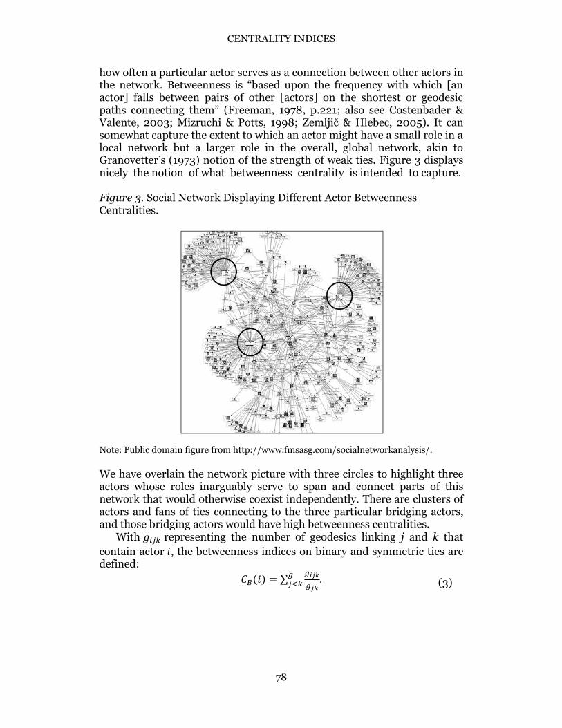
how often a particular actor serves as a connection between other actors in the network. Betweenness is “based upon the frequency with which [an actor] falls between pairs of other [actors] on the shortest or geodesic paths connecting them” (Freeman, 1978, p.221; also see Costenbader & Valente, 2003; Mizruchi & Potts, 1998; Zemljič & Hlebec, 2005). It can somewhat capture the extent to which an actor might have a small role in a local network but a larger role in the overall, global network, akin to Granovetter’s (1973) notion of the strength of weak ties. Figure 3 displays nicely the notion of what betweenness centrality is intended to capture. Figure 3. Social Network Displaying Different Actor Betweenness Centralities.

Note: Public domain figure from http://www.fmsasg.com/socialnetworkanalysis/.

We have overlain the network picture with three circles to highlight three actors whose roles inarguably serve to span and connect parts of this network that would otherwise coexist independently. There are clusters of actors and fans of ties connecting to the three particular bridging actors, and those bridging actors would have high betweenness centralities.

With 𝑔𝑖𝑗𝑘 representing the number of geodesics linking j and k that

contain actor 𝑖, the betweenness indices on binary and symmetric ties are defined:

𝐶𝐵(𝑖) = ∑𝑔𝑖𝑗𝑘

𝑔𝑗𝑘

𝑔𝑗<𝑘 .

(3)

IACOBUCCI

79

The maximum value for the betweenness index is [(𝑔 − 1)(𝑔 − 2)]/2, so

this centrality index is normed as 𝐶′𝐵(𝑖) =2𝐶𝐵(𝑖)

(𝑔−1)(𝑔−2)=

2𝐶𝐵(𝑖)

𝑔2−3𝑔+2.

Eigenvector. The fourth centrality index that is commonly provided in

software packages and therefore worthy of inclusion in this consideration is the set of values contained in the first eigenvector of the adjacency matrix (the vector associated with the largest eigenvalue). Stated simply, actors get more “centrality credit” for being connected to other actors who are themselves well-connected. Bonacich (1972), building on Katz (1953), proposed that the first eigenvector of an adjacency matrix could serve as a centrality measure that would capture patterns of direct and indirect connections (also see Borgatti, Carley, & Krackhardt, 2006). Bonacich’s (1972) idea was that the eigenvectors (of symmetric sociomatrices and singular value decompositions of asymmetric sociomatrices) would capture the differential weighting of ties to partners who themselves are highly vs. less central. Specifically, ties are weighted more heavily when linked to actors who themselves are more central.

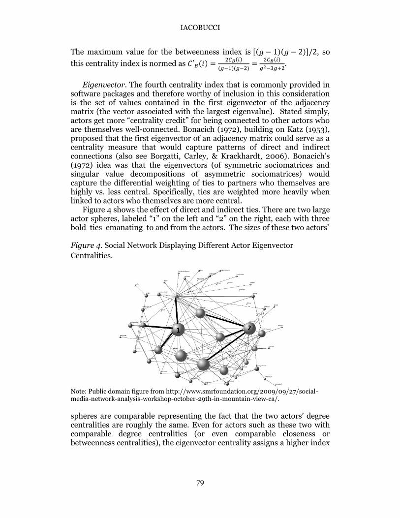
Figure 4 shows the effect of direct and indirect ties. There are two large actor spheres, labeled “1” on the left and “2” on the right, each with three bold ties emanating to and from the actors. The sizes of these two actors’ Figure 4. Social Network Displaying Different Actor Eigenvector

Centralities.

Note: Public domain figure from http://www.smrfoundation.org/2009/09/27/social-media-network-analysis-workshop-october-29th-in-mountain-view-ca/.

spheres are comparable representing the fact that the two actors’ degree centralities are roughly the same. Even for actors such as these two with comparable degree centralities (or even comparable closeness or betweenness centralities), the eigenvector centrality assigns a higher index

CENTRALITY INDICES

80

to an actor like “2” who is connected to many actors who are themselves highly inter-connected and represented by larger nodes. Actor “1” would have a smaller eigenvector centrality index because this actor is connected to other actors in the network who are less inter-connected themselves. (For a brief refresher on eigenvector centralities, please see the Appendix.)

With those illustrations of an eigenvector centrality’s conceptual meaning, let us now define it. For the sociomatrix X, the eigen-decomposition into an eigenvector, v, and eigenvalue, 𝜆, is reflected in the familiar equation:

𝑿𝒗 = 𝜆𝒗.

The eigenvector score for actor 𝑖 is 𝐶𝐸𝑉(𝑖) , a weighted function of the statuses of the other actors to whom actor 𝑖 is connected: 𝐶𝐸𝑉(𝑖) = 𝑥1𝑖𝑣1 +𝑥2𝑖𝑣2 + ⋯+ 𝑥𝑔𝑖𝑣𝑔.

Centrality indices based on eigenvectors have become quite popular and serve as the basis for numerous other indices, such as Bonacich’s power index (1987; 2007) and Google’s Page Rank index (Brin & Page, 1998; Friedkin & Johnsen, 1990). The model has been expanded, such as finessing parameters to weight indirect ties to a greater or lesser extent (Bonacich, 1987). Next, in Study 1, we examine the empirical performance of these four centrality indices on small social networks with exemplar structures, stylized networks drawn from the literature. Given the conceptual foundations of the centrality indices, network scholars might expect certain indices to be more meaningful for reflecting certain distinct structures.

Study 1: Performance of the Centralities on Small, Stylized Networks

To understand the nature of the likely differences among the centrality

indices, it should be useful to begin with small, simple example networks (rather than the real and complex networks captured in Figure 1 through 4). Thus, in Figure 5 we have depicted social networks with prototypical structures that have been used to inform the conceptual development of many social networks analytics, from centrality indices to definitions of cliques and stochastic equivalence. These are stylized networks that we will use to establish whether the theoretically distinct underpinnings of the different centrality indices are manifest in their empirical performance in the descriptive statistics. Figure 5 also shows the relationships among these stylized networks.

(4)

IACOBUCCI

81

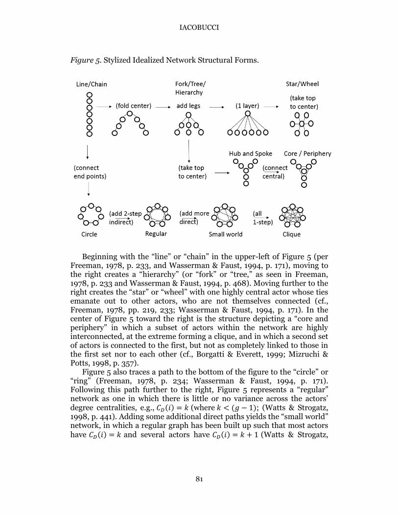
Figure 5. Stylized Idealized Network Structural Forms.

Beginning with the “line” or “chain” in the upper-left of Figure 5 (per Freeman, 1978, p. 233, and Wasserman & Faust, 1994, p. 171), moving to the right creates a “hierarchy” (or “fork” or “tree,” as seen in Freeman, 1978, p. 233 and Wasserman & Faust, 1994, p. 468). Moving further to the right creates the “star” or “wheel” with one highly central actor whose ties emanate out to other actors, who are not themselves connected (cf., Freeman, 1978, pp. 219, 233; Wasserman & Faust, 1994, p. 171). In the center of Figure 5 toward the right is the structure depicting a “core and periphery” in which a subset of actors within the network are highly interconnected, at the extreme forming a clique, and in which a second set of actors is connected to the first, but not as completely linked to those in the first set nor to each other (cf., Borgatti & Everett, 1999; Mizruchi & Potts, 1998, p. 357).

Figure 5 also traces a path to the bottom of the figure to the “circle” or “ring” (Freeman, 1978, p. 234; Wasserman & Faust, 1994, p. 171). Following this path further to the right, Figure 5 represents a “regular” network as one in which there is little or no variance across the actors’ degree centralities, e.g., 𝐶𝐷(𝑖) = 𝑘 (where 𝑘 < (𝑔 − 1); (Watts & Strogatz, 1998, p. 441). Adding some additional direct paths yields the “small world” network, in which a regular graph has been built up such that most actors have 𝐶𝐷(𝑖) = 𝑘 and several actors have 𝐶𝐷(𝑖) = 𝑘 + 1 (Watts & Strogatz,

CENTRALITY INDICES

82

1998, p. 441). Finally in Figure 5, at the lower-right is the “clique,” traditionally defined as a maximally connected subgraph within the network, wherein each actor’s degree centrality is its maximum value, 𝐶𝐷(𝑖) = 𝑔 − 1 (Freeman, 1978, p. 236; Knoke & Yang, 2007, p. 67; Scott 2012, p. 113).

Given these structures, it would not seem unreasonable to anticipate that some centrality indices may be more sensitive to reflecting certain elements of different network structure. For example, one might expect cliques (lower right) to have high degrees, and high closeness, but low betweenness. In contrast, networks in the forms of lines and hierarchies (upper left) might yield greater betweenness indices. To examine whether these relationships hold, we analyzed each network to obtain all four sets of centralities. (For simplicity, we constructed the adjacency matrices to be binary and symmetric.) We then computed the means and standard deviations of these centralities across the actors within a given network. Figures 6 through 9 depict these means and standard deviations for each stylized network, for each centrality index.

Results for Study 1

Means and Standard Deviations

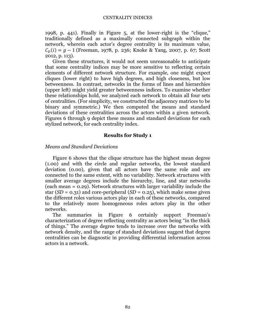
Figure 6 shows that the clique structure has the highest mean degree (1.00) and with the circle and regular networks, the lowest standard deviation (0.00), given that all actors have the same role and are connected to the same extent, with no variability. Network structures with smaller average degrees include the hierarchy, line, and star networks (each mean = 0.29). Network structures with larger variability include the star (SD = 0.31) and core-peripheral (SD = 0.25), which make sense given the different roles various actors play in each of these networks, compared to the relatively more homogeneous roles actors play in the other networks.

The summaries in Figure 6 certainly support Freeman’s characterization of degree reflecting centrality as actors being “in the thick of things.” The average degree tends to increase over the networks with network density, and the range of standard deviations suggest that degree centralities can be diagnostic in providing differential information across actors in a network.

IACOBUCCI

83

Figure 6. Degree Centralities Normalized: Means and Standard Deviations.

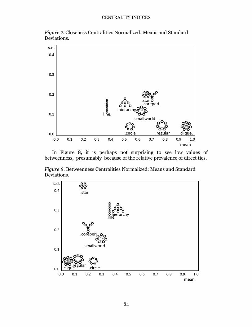
Figure 7 shows some variability among the networks in terms of their

average closeness indices, and relatively compressed variability in terms of the standard deviations of the actor indices within the networks. The two extreme means in Figure 7 depict nicely the characteristic captured by closeness. The clique mean is high (1.00, and SD = 0.00) because every actor is directly connected to all other actors, thus all actors are very close to one another. The line mean is the lowest (0.39) because while adjacent actors are near each other, the actors toward the ends must traverse through 2- or 3-length ties or longer. Thus as a whole, the actors in the line network have lower average closeness centralities.

CENTRALITY INDICES

84

Figure 7. Closeness Centralities Normalized: Means and Standard Deviations.

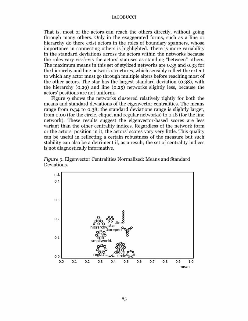
In Figure 8, it is perhaps not surprising to see low values of

betweenness, presumably because of the relative prevalence of direct ties.

Figure 8. Betweenness Centralities Normalized: Means and Standard Deviations.

IACOBUCCI

85

That is, most of the actors can reach the others directly, without going through many others. Only in the exaggerated forms, such as a line or hierarchy do there exist actors in the roles of boundary spanners, whose importance in connecting others is highlighted. There is more variability in the standard deviations across the actors within the networks because the roles vary vis-à-vis the actors’ statuses as standing “between” others. The maximum means in this set of stylized networks are 0.35 and 0.33 for the hierarchy and line network structures, which sensibly reflect the extent to which any actor must go through multiple alters before reaching most of the other actors. The star has the largest standard deviation (0.38), with the hierarchy (0.29) and line (0.25) networks slightly less, because the actors’ positions are not uniform.

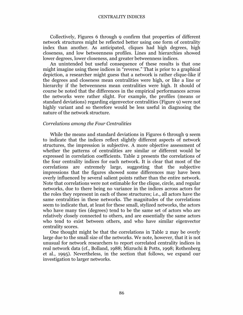
Figure 9 shows the networks clustered relatively tightly for both the means and standard deviations of the eigenvector centralities. The means range from 0.34 to 0.38; the standard deviations range is slightly larger, from 0.00 (for the circle, clique, and regular networks) to 0.18 (for the line network). These results suggest the eigenvector-based scores are less variant than the other centrality indices. Regardless of the network form or the actors’ position in it, the actors’ scores vary very little. This quality can be useful in reflecting a certain robustness of the measure but such stability can also be a detriment if, as a result, the set of centrality indices is not diagnostically informative.

Figure 9. Eigenvector Centralities Normalized: Means and Standard Deviations.

CENTRALITY INDICES

86

Collectively, Figures 6 through 9 confirm that properties of different

network structures might be reflected better using one form of centrality index than another. As anticipated, cliques had high degrees, high closeness, and low betweenness profiles. Lines and hierarchies showed lower degrees, lower closeness, and greater betweenness indices.

An unintended but useful consequence of these results is that one might imagine using these indices in “reverse.” That is prior to a graphical depiction, a researcher might guess that a network is rather clique-like if the degrees and closeness mean centralities were high, or like a line or hierarchy if the betweenness mean centralities were high. It should of course be noted that the differences in the empirical performances across the networks were rather slight. For example, the profiles (means or standard deviations) regarding eigenvector centralities (Figure 9) were not highly variant and so therefore would be less useful in diagnosing the nature of the network structure.

Correlations among the Four Centralities

While the means and standard deviations in Figures 6 through 9 seem to indicate that the indices reflect slightly different aspects of network structures, the impression is subjective. A more objective assessment of whether the patterns of centralities are similar or different would be expressed in correlation coefficients. Table 2 presents the correlations of the four centrality indices for each network. It is clear that most of the correlations are extremely large, suggesting that the subjective impressions that the figures showed some differences may have been overly influenced by several salient points rather than the entire network. Note that correlations were not estimable for the clique, circle, and regular networks, due to there being no variance in the indices across actors for the roles they represent in each of these structures; i.e., all actors have the same centralities in these networks. The magnitudes of the correlations seem to indicate that, at least for these small, stylized networks, the actors who have many ties (degrees) tend to be the same set of actors who are relatively closely connected to others, and are essentially the same actors who tend to exist between others, and who have similar eigenvector centrality scores.

One thought might be that the correlations in Table 2 may be overly large due to the small size of the networks. We note, however, that it is not unusual for network researchers to report correlated centrality indices in real network data (cf., Bolland, 1988; Mizruchi & Potts, 1998; Rothenberg et al., 1995). Nevertheless, in the section that follows, we expand our investigation to larger networks.

IACOBUCCI

87

Table 2 Correlations among Four Centrality Indices for Stylized Networks

Network Line Clique degree close between eigenv degree close between eigenv

Degree 1.000 Closeness 0.844 1.000 all SD = 0, so n/a Betweenness 0.913 0.989 1.000 Eigenvector 0.900 0.993 0.999 1.000 Hierarchy Star degree close between eigenv degree close between eigenv Degree 1.000 1.000 Closeness 0.999 1.000 1.000 1.000 Betweenness 0.993 0.997 1.000 1.000 1.000 1.000 Eigenvector 1.000 0.999 0.993 1.000 1.000 1.000 1.000 1.000

Circle Core-Peripheral degree close between eigenv degree close between eigenv

Degree 1.000 Closeness all SD = 0, so n/a 0.999 1.000 Betweenness 0.884 0.868 1.000 Eigenvector 0.987 0.991 0.795 1.000

Regular Small World degree close between eigenv degree close between eigenv

Degree 1.000 Closeness all SD = 0, so n/a 0.963 1.000 Betweenness 0.969 0.999 1.000 Eigenvector 0.941 0.895 0.902 1.000

Study 2: Extending the Stylized Networks in Size: 3 g and 3 Replications

While the results on the stylized networks from Study 1 provide a basic

level of information that the four centrality indices can seem to have some distinct patterns (in their means and standard deviations), and yet show some commonalities (i.e., high correlations), the analyses may be somewhat limited due to the small size of the networks. Such small networks have certainly been used throughout the literature to demonstrate concepts about network structure (cf., Wasserman & Faust, 1994), but 𝑔 = 7 is not as large as some of the classic networks that scholars have analyzed in the social network literature, such as the 32 actors in Freeman’s EIES (electronic information exchange system) network (Freeman & Freeman, 1979), Krackhardt’s 21 high-tech managers (Krackhardt, 1987), Sampson’s 18 monks (Sampson, 1968), or Newcomb’s 17 freshmen (Newcomb, 1961).

Thus, in this study, we examine the means, standard deviations, and correlations among the four centrality indices, on larger networks, for a subset of the stylized networks. Given the span of the means and standard deviations represented across the hierarchy, star, and core-periphery, we

CENTRALITY INDICES

88

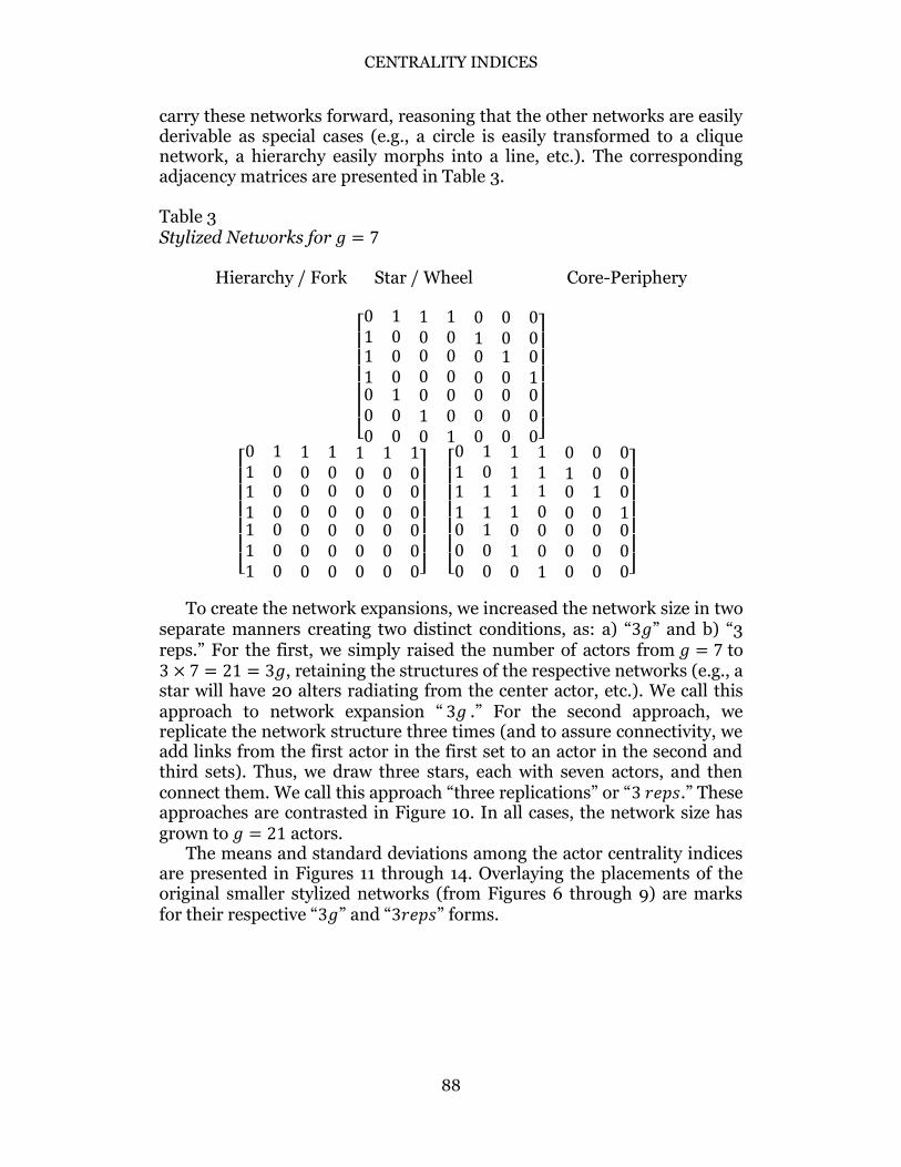
carry these networks forward, reasoning that the other networks are easily derivable as special cases (e.g., a circle is easily transformed to a clique network, a hierarchy easily morphs into a line, etc.). The corresponding adjacency matrices are presented in Table 3.

Table 3 Stylized Networks for 𝑔 = 7

Hierarchy / Fork Star / Wheel Core-Periphery

[ 0 1 1 1 0 0 01 0 0 0 1 0 011000

00100

0 0 0 1 00 0 0 0 1010

001

0 0 00 0 00 0 0]

[ 0 1 1 1 1 1 11 0 0 0 0 0 011111

00000

0 0 0 0 00 0 0 0 0000

000

0 0 00 0 00 0 0]

[ 0 1 1 1 0 0 01 0 1 1 1 0 011000

11100

1 1 0 1 01 0 0 0 1010

001

0 0 00 0 00 0 0]

To create the network expansions, we increased the network size in two

separate manners creating two distinct conditions, as: a) “3𝑔” and b) “3 reps.” For the first, we simply raised the number of actors from 𝑔 = 7 to 3 × 7 = 21 = 3𝑔, retaining the structures of the respective networks (e.g., a star will have 20 alters radiating from the center actor, etc.). We call this approach to network expansion “ 3𝑔 .” For the second approach, we replicate the network structure three times (and to assure connectivity, we add links from the first actor in the first set to an actor in the second and third sets). Thus, we draw three stars, each with seven actors, and then connect them. We call this approach “three replications” or “3 𝑟𝑒𝑝𝑠.” These approaches are contrasted in Figure 10. In all cases, the network size has grown to 𝑔 = 21 actors.

The means and standard deviations among the actor centrality indices are presented in Figures 11 through 14. Overlaying the placements of the original smaller stylized networks (from Figures 6 through 9) are marks for their respective “3𝑔” and “3𝑟𝑒𝑝𝑠” forms.

IACOBUCCI

89

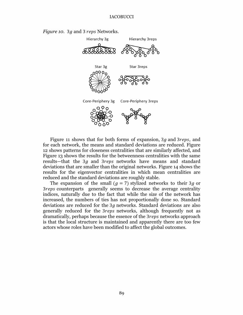
Figure 10. 3𝑔 and 3 𝑟𝑒𝑝𝑠 Networks.

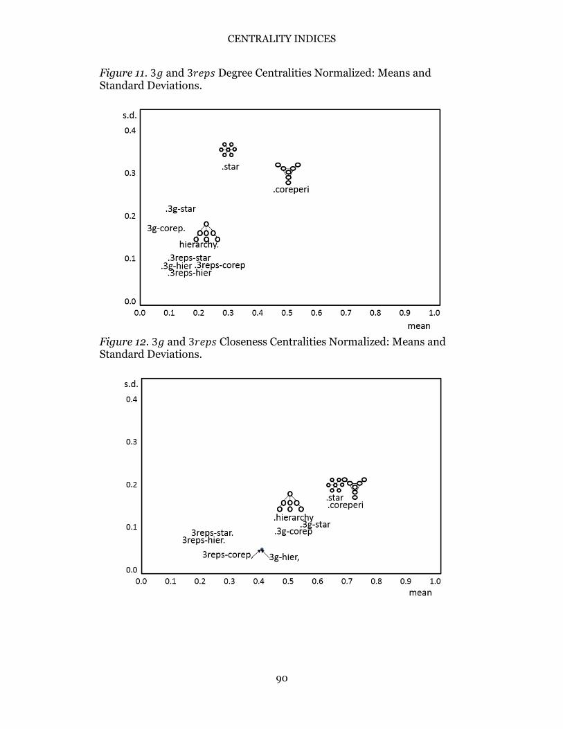
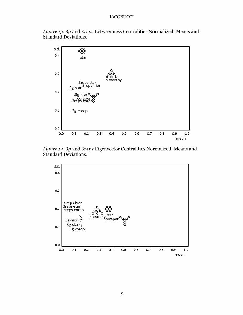
Figure 11 shows that for both forms of expansion, 3𝑔 and 3𝑟𝑒𝑝𝑠, and for each network, the means and standard deviations are reduced. Figure 12 shows patterns for closeness centralities that are similarly affected, and Figure 13 shows the results for the betweenness centralities with the same results—that the 3𝑔 and 3𝑟𝑒𝑝𝑠 networks have means and standard deviations that are smaller than the original networks. Figure 14 shows the results for the eigenvector centralities in which mean centralities are reduced and the standard deviations are roughly stable.

The expansion of the small (𝑔 = 7) stylized networks to their 3𝑔 or 3𝑟𝑒𝑝𝑠 counterparts generally seems to decrease the average centrality indices, naturally due to the fact that while the size of the network has increased, the numbers of ties has not proportionally done so. Standard deviations are reduced for the 3𝑔 networks. Standard deviations are also generally reduced for the 3𝑟𝑒𝑝𝑠 networks, although frequently not as dramatically, perhaps because the essence of the 3𝑟𝑒𝑝𝑠 networks approach is that the local structure is maintained and apparently there are too few actors whose roles have been modified to affect the global outcomes.

CENTRALITY INDICES

90

Figure 11. 3𝑔 and 3𝑟𝑒𝑝𝑠 Degree Centralities Normalized: Means and Standard Deviations.

Figure 12. 3𝑔 and 3𝑟𝑒𝑝𝑠 Closeness Centralities Normalized: Means and Standard Deviations.

IACOBUCCI

91

Figure 13. 3𝑔 and 3𝑟𝑒𝑝𝑠 Betweenness Centralities Normalized: Means and Standard Deviations.

Figure 14. 3𝑔 and 3𝑟𝑒𝑝𝑠 Eigenvector Centralities Normalized: Means and Standard Deviations.

CENTRALITY INDICES

92

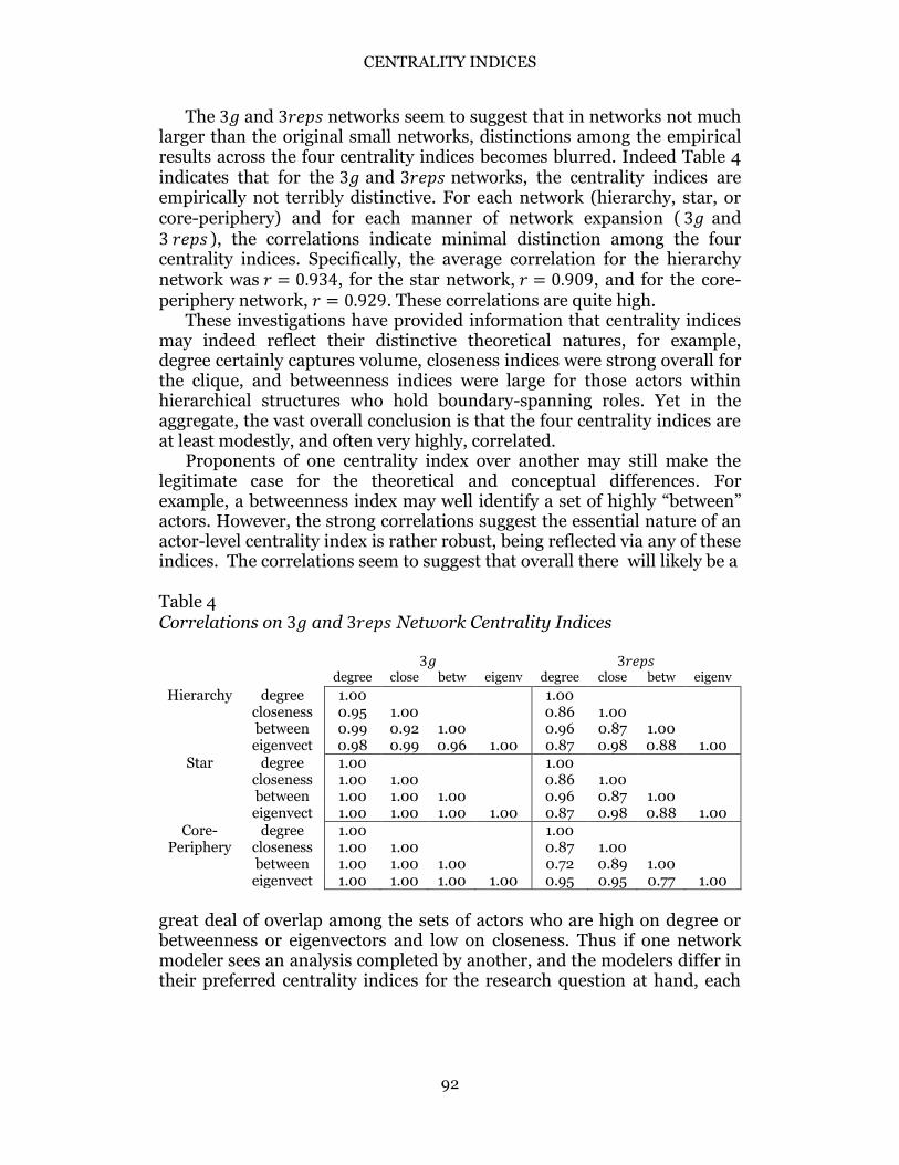
The 3𝑔 and 3𝑟𝑒𝑝𝑠 networks seem to suggest that in networks not much larger than the original small networks, distinctions among the empirical results across the four centrality indices becomes blurred. Indeed Table 4 indicates that for the 3𝑔 and 3𝑟𝑒𝑝𝑠 networks, the centrality indices are empirically not terribly distinctive. For each network (hierarchy, star, or core-periphery) and for each manner of network expansion ( 3𝑔 and 3 𝑟𝑒𝑝𝑠 ), the correlations indicate minimal distinction among the four centrality indices. Specifically, the average correlation for the hierarchy network was 𝑟 = 0.934, for the star network, 𝑟 = 0.909, and for the core-periphery network, 𝑟 = 0.929. These correlations are quite high.

These investigations have provided information that centrality indices may indeed reflect their distinctive theoretical natures, for example, degree certainly captures volume, closeness indices were strong overall for the clique, and betweenness indices were large for those actors within hierarchical structures who hold boundary-spanning roles. Yet in the aggregate, the vast overall conclusion is that the four centrality indices are at least modestly, and often very highly, correlated. Proponents of one centrality index over another may still make the legitimate case for the theoretical and conceptual differences. For example, a betweenness index may well identify a set of highly “between” actors. However, the strong correlations suggest the essential nature of an actor-level centrality index is rather robust, being reflected via any of these indices. The correlations seem to suggest that overall there will likely be a

Table 4 Correlations on 3𝑔 and 3𝑟𝑒𝑝𝑠 Network Centrality Indices

3𝑔 3𝑟𝑒𝑝𝑠 degree close betw eigenv degree close betw eigenv

Hierarchy degree 1.00 1.00 closeness 0.95 1.00 0.86 1.00 between 0.99 0.92 1.00 0.96 0.87 1.00 eigenvect 0.98 0.99 0.96 1.00 0.87 0.98 0.88 1.00

Star degree 1.00 1.00 closeness 1.00 1.00 0.86 1.00 between 1.00 1.00 1.00 0.96 0.87 1.00 eigenvect 1.00 1.00 1.00 1.00 0.87 0.98 0.88 1.00

Core- degree 1.00 1.00 Periphery closeness 1.00 1.00 0.87 1.00

between 1.00 1.00 1.00 0.72 0.89 1.00 eigenvect 1.00 1.00 1.00 1.00 0.95 0.95 0.77 1.00

great deal of overlap among the sets of actors who are high on degree or betweenness or eigenvectors and low on closeness. Thus if one network modeler sees an analysis completed by another, and the modelers differ in their preferred centrality indices for the research question at hand, each

IACOBUCCI

93

could take some solace in knowing that the conclusions that would be drawn would not likely to vary much, from analysis to analysis, across centrality index to centrality index.

Study 3: Computing Time

Next, we consider a practical concern. If a battery of centrality indices are sufficiently correlated that they provide the network analyst with essentially the same information, then a choice among the centrality indices may be motivated by a different criterion. For example, with the enormous size of many of today’s online networks, it may be prudent to select the network indices that are computationally efficient (e.g., fast). While today’s large networks may exacerbate such a search, this concern for computational efficiencies has existed for some time (cf., Bader & Madduri, 2006; Poulin, Boily, & Mâsse, 2000).

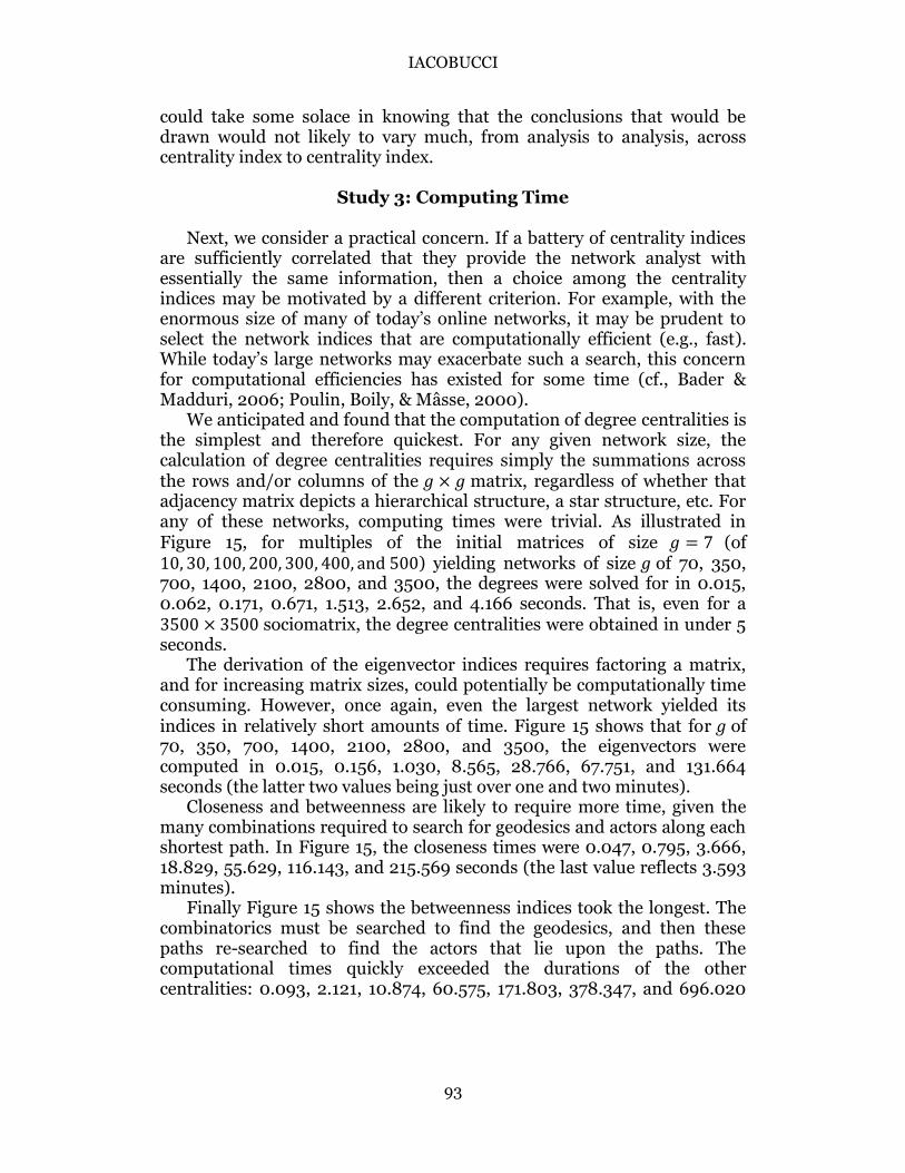
We anticipated and found that the computation of degree centralities is the simplest and therefore quickest. For any given network size, the calculation of degree centralities requires simply the summations across the rows and/or columns of the 𝑔 × 𝑔 matrix, regardless of whether that adjacency matrix depicts a hierarchical structure, a star structure, etc. For any of these networks, computing times were trivial. As illustrated in Figure 15, for multiples of the initial matrices of size 𝑔 = 7 (of 10, 30, 100, 200, 300, 400, and 500) yielding networks of size 𝑔 of 70, 350, 700, 1400, 2100, 2800, and 3500, the degrees were solved for in 0.015, 0.062, 0.171, 0.671, 1.513, 2.652, and 4.166 seconds. That is, even for a 3500 × 3500 sociomatrix, the degree centralities were obtained in under 5 seconds.

The derivation of the eigenvector indices requires factoring a matrix, and for increasing matrix sizes, could potentially be computationally time consuming. However, once again, even the largest network yielded its indices in relatively short amounts of time. Figure 15 shows that for 𝑔 of 70, 350, 700, 1400, 2100, 2800, and 3500, the eigenvectors were computed in 0.015, 0.156, 1.030, 8.565, 28.766, 67.751, and 131.664 seconds (the latter two values being just over one and two minutes).

Closeness and betweenness are likely to require more time, given the many combinations required to search for geodesics and actors along each shortest path. In Figure 15, the closeness times were 0.047, 0.795, 3.666, 18.829, 55.629, 116.143, and 215.569 seconds (the last value reflects 3.593 minutes).

Finally Figure 15 shows the betweenness indices took the longest. The combinatorics must be searched to find the geodesics, and then these paths re-searched to find the actors that lie upon the paths. The computational times quickly exceeded the durations of the other centralities: 0.093, 2.121, 10.874, 60.575, 171.803, 378.347, and 696.020

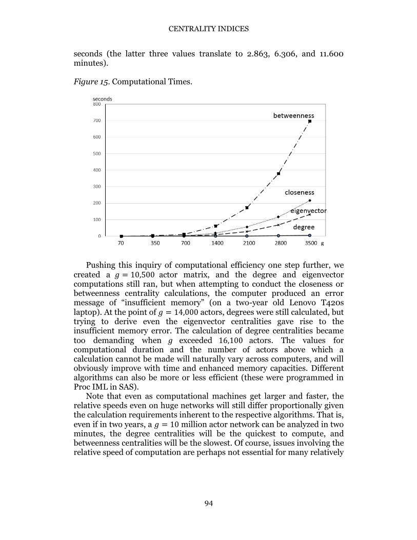
CENTRALITY INDICES

94

seconds (the latter three values translate to 2.863, 6.306, and 11.600 minutes). Figure 15. Computational Times.

Pushing this inquiry of computational efficiency one step further, we

created a 𝑔 = 10,500 actor matrix, and the degree and eigenvector computations still ran, but when attempting to conduct the closeness or betweenness centrality calculations, the computer produced an error message of “insufficient memory” (on a two-year old Lenovo T420s laptop). At the point of 𝑔 = 14,000 actors, degrees were still calculated, but trying to derive even the eigenvector centralities gave rise to the insufficient memory error. The calculation of degree centralities became too demanding when 𝑔 exceeded 16,100 actors. The values for computational duration and the number of actors above which a calculation cannot be made will naturally vary across computers, and will obviously improve with time and enhanced memory capacities. Different algorithms can also be more or less efficient (these were programmed in Proc IML in SAS).

Note that even as computational machines get larger and faster, the relative speeds even on huge networks will still differ proportionally given the calculation requirements inherent to the respective algorithms. That is, even if in two years, a 𝑔 = 10 million actor network can be analyzed in two minutes, the degree centralities will be the quickest to compute, and betweenness centralities will be the slowest. Of course, issues involving the relative speed of computation are perhaps not essential for many relatively

IACOBUCCI

95

small applied network questions, but they do seem relevant for inquiries into structures in today’s massive online networks.

Discussion This research considered several aspects of four key centrality indices: degree, closeness, betweenness, and eigenvectors. Study 1 focused on clean forms of stylized networks expected to exemplify those conditions under which the specific particular sensitivities of the four centralities should be most distinct. Depending on the nature and content of the relational ties, some centrality indices may be more meaningful or applicable than others. For example, if the network connections reflect flows of ties seeking the efficiencies of shortest paths, then closeness and betweenness may seem optimal given that they are based on geodesics (Borgatti 2005). By comparison, degree and eigenvector-based centralities may be better in characterizing volumes of ties (Borgatti & Everett, 2005). The profiles of the four centralities did indeed show some distinctiveness, at least in terms of means and standard deviations. However, the four centralities were, on the whole, rather highly correlated. The high correlations suggest overall commonality, which in turn suggests the choice of a centrality index is not highly critical when characterizing a network. It is not unusual in studies of real social network data for centrality indices to be rather highly correlated. For example, Rothenberg et al. (1995, p.293) found correlations averaging 0.62 to 0.87, and concluded that, “The measures appear equivalent, for the most part, although further analysis in other contexts may sharpen our insight.”

We also tested computing times and found that degree centralities could be calculated extremely quickly, and eigenvector centralities took only a little longer. Given the combinatorics involved in calculating closeness and betweenness, they took longer, with betweenness computational times in particular rising quickly. The fact that the centrality indices are rather highly correlated may be interpreted as good news: it does not abate the conceptual distinctions; rather, it suggests that the indices proffer similar information about actors in networks. This robustness is reassuring given the many network analysts working in application areas who may not appreciate the theoretically distinct origins. While we aimed to be fairly inclusive of exemplar network structures, future research might consider the extent to which these findings are upheld in still more network structures. For example, many real world networks are very large and quite sparse in many local regions of the network. We expect that our findings (descriptives and moderate to high correlations among the four centrality indices) should largely replicate, in part because sparse networks by definition contain numerous isolates or

CENTRALITY INDICES

96

actors with relatively few connections. Hence their impact on summary statistics is not likely to be extensive. With this research, we hope to have contributed to a deeper understanding of four of the most frequently used centrality indices. Network modelers can still of course continue to select among indices based on conceptual fit, such as focusing on betweenness centralities when the purposes of the research is to identify actors within the network who serve as interim conduits. That is, we respect and are not negating the important conceptual differences between the centralities and what they are designed to reflect. Yet the emphasis in our research was on the indices’ empirical performance, and our results showed that they were generally rather highly correlated. These results might seem counter to theoretically-based normative advice about when to use which centrality index, yet we interpret the findings as perhaps paradoxically good news in that network researchers can be confident that if a network structure has a story to tell, in all likelihood, it will be told regardless of the specific centrality index implemented for its detection.

Author notes: Dawn Iacobucci (corresponding author): Vanderbilt University, 401 21st Avenue South, Nashville, TN, 32703, dawn.iacobucci@owen.vanderbilt.edu. Rebecca McBride, Finance and Administration Development Manager at Deloitte, becanya@hotmail.com. Diedre L. Popovich, Texas Tech University, Lubbock, TX, 79409, deidre.popovich@ttu.edu. Maria Rouziou, Wilfrid Laurier University, Ontario, CA, mrouziou@wlu.ca.

References

Bader, D. A. & Madduri, K. (2006). Parallel Algorithms for Evaluating Centrality Indices in Real-world Networks. International Conference on Parallel Processing, 539-550.

Bolland, J. M. (1988). Sorting Out Centrality: An Analysis of the Performance of Four Centrality Models in Real and Simulated Networks. Social Networks, 10, 233-253.

Bonacich, P. (1972). Factoring and Weighting Approaches to Status Scores and Clique Identification. Journal of Mathematical Sociology, 2, 113-120.

Bonacich, P. (1987). Power and Centrality: A Family of Measures. American Journal of Sociology, 92, 1170-1182.

Bonacich, P. (2007). Some Unique Properties of Eigenvector Centrality. Social Networks, 29, 555-564.

Borgatti, S. (2005). Centrality and Network Flow. Social Networks, 27, 55-71. Borgatti, S., Carley, K. M. & Krackhardt, D. (2006). On the Robustness of

Centrality Measures under Conditions of Imperfect Data. Social Networks, 28, 124-136.

IACOBUCCI

97

Borgatti, S. & Everett, M. (1999). Models of Core/Periphery Structures. Social Networks, 21, 375-395.

Borgatti, S. & Everett, M. (2005). A Graph-Theoretic Perspective on Centrality. Social Networks, 28, 466-484.

Brass, D. J. (1984), Being in the Right Place: A Structural Analysis of Individual Influence in an Organization. Administrative Science Quarterly, 29, 518-539.

Brin, S. & Page, L. (1998). The Anatomy of a Large-Scale Hypertextual Web Search Engine. Computer Networks and ISDN Systems, 30, 107-117.

Costenbader, E. & Valente, T. W. (2003). The Stability of Centrality Measures When Networks are Sampled. Social Networks, 25, 283-307.

Everett, M. G. & Borgatti, S. P. (1999). The Centrality of Groups and Classes,” Journal of Mathematical Sociology, 23, 181-202.

Ferrara, E., De Meo, P., Catanese, S. & Fiumara, G. (2014). Detecting Criminal Organizations in Mobile Phone Networks. Expert Systems with Applications, 41, 5733-5750.

Freeman, L. (1978/1979). Centrality in Networks: Conceptual Clarification. Social Networks, 1, 215-239.

Freeman, L. C., Borgatti, S. P. & White, D. R. (1991). Centrality in Valued Graphs: A Measure of Betweenness Based on Network Flow. Social Networks, 13, 141-154.

Freeman, S. C., & Freeman, L. C. (1979). The Networkers Network: A Study of the Impact of a New Communication Medium on Sociometric Structure. Social Science Research Reports No. 46, Irvine, CA, University of California.

Friedkin, N. E. (1991). Theoretical Foundations for Centrality Measures. American Journal of Sociology, 96, 1478-1504.

Friedkin, N. E. & Johnsen, E. C. (1990). Social Influence and Opinions. Journal of Mathematical Sociology, 15, 193-206.

Granovetter, Mark S. (1973). The Strength of Weak Ties. American Journal of Sociology, 78, 1360-1380.

Katz, L. (1953). A New Status Index Derived from Sociometric Analysis. Psychometrika, 18, 39–43.

Knoke, D. & Yang, S. (2007), Social Network Analysis, 2nd ed., Los Angeles, CA: Sage.

Koschmann, M. A. & Wanberg, J. (2016). Assessing the Effectiveness of Collaborative Interorganizational Networks Through Client Communication. Communication Research Reports, 33, 253-258.

Krackhardt, D. (1987). Cognitive Social Structures. Social Networks, 9, 104-134. Mizruchi, M. S. & Potts, B. B. (1998). Centrality and Power Revisited: Actor

Success in Group Decision Making. Social Networks, 20, 353–387. Newcomb, T. (1961). The Acquaintance Process, New York: Holt, Rinehart, and

Winston. O’Kelly, M. (2016). Global Airline Networks: Comparative Nodal Access

Measures. Spatial Economic Analysis, 11, 253-275. Opsahl, T., Agneessens, F., & Skvoretz, J. (2002). Node Centrality in Weighted

Networks: Generalizing Degree and Shortest Paths. Social Networks, 32, 245-251.

Poulin, R., Boily, M.-C., & Mâsse, B. R. (2000). Dynamical Systems to Define Centrality in Social Networks. Social Networks, 22, 187–220.

CENTRALITY INDICES

98

Rothenberg, R. B., Potterat, J. J., Woodhouse, D. E., Darrow, W. W., Muth, S. Q., & Klovdahl, A. S. (1995). Choosing a Centrality Measure: Epidemiologic Correlates in the Colorado Springs Study of Social Networks.. Social Networks, 17, 273-297.

Rubinov, M. & Sporns, O. (2010). Complex Network Measures of Brain Connectivity: Uses and Interpretations. NeuroImage, 52, 1059-1069.

Sabate, F., Berbegal-Mirabent, J., Canabate, A., & Lebherz, P. R. (2014). Factors Influencing Popularity of Branded Content in Facebook Fan Pages. European Management Journal, 32, 1001-1011.

Sampson, S. F. (1968). A Novitiate in a Period of Change: An Experimental and Case Study of Social Relationships. Dissertation, Cornell University.

Scott, J. (2012), Social Network Analysis, 3rd ed., Los Angeles: Sage. Smith, J. A. & Moody, J. (2013). Structural Effects of Network Sampling Coverage

I: Nodes Missing at Random. Social Networks, 35, 652-668. Stephenson, K. & Zelen, M. (1989). Rethinking Centrality: Methods and

Examples. Social Networks, 11, 1-37. Wasserman, S., & Faust, K. (1994), Social Network Analysis: Methods and

Applications, New York: Cambridge University Press. Watts, D. J. & Strogatz, S. H. (1998). Collective Dynamics of ‘Small-World’

Networks. Letters to Nature, 393, 440-442. Wey, T., Blumstein, D. T., Shen, W., & Jordan, F. (2008). Social Network

Analysis of Animal Behaviour: A Promising Tool for the Study of Sociality. Animal Behaviour, 75, 333-344.

White, D. R. & Borgatti, S. P. (1994). Betweenness Centrality Measures for Directed Graphs. Social Networks, 16, 335-346.

Zemljič, B. & Hlebec, V. (2005). Reliability of Measures of Centrality and Prominence.. Social Networks, 27, 73-88.

Zhang, X., Chen, X., Chen, Y., Wang, S., Li, Z., & Xia, J. (2015). Event Detection and Popularity Prediction in Microblogging.. Neurocomputing, 149, 1469-1480.

IACOBUCCI

99

Appendix: Brief Refresher of Eigenvector Centrality

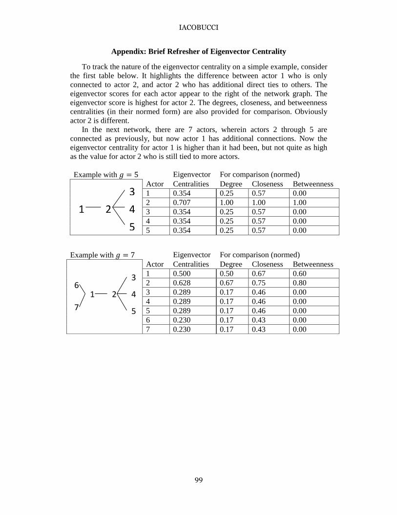
To track the nature of the eigenvector centrality on a simple example, consider

the first table below. It highlights the difference between actor 1 who is only

connected to actor 2, and actor 2 who has additional direct ties to others. The

eigenvector scores for each actor appear to the right of the network graph. The

eigenvector score is highest for actor 2. The degrees, closeness, and betweenness

centralities (in their normed form) are also provided for comparison. Obviously

actor 2 is different.

In the next network, there are 7 actors, wherein actors 2 through 5 are

connected as previously, but now actor 1 has additional connections. Now the

eigenvector centrality for actor 1 is higher than it had been, but not quite as high

as the value for actor 2 who is still tied to more actors.

Example with 𝑔 = 5 Eigenvector For comparison (normed)

Actor Centralities Degree Closeness Betweenness

1 0.354 0.25 0.57 0.00

2 0.707 1.00 1.00 1.00

3 0.354 0.25 0.57 0.00

4 0.354 0.25 0.57 0.00

5 0.354 0.25 0.57 0.00

Example with 𝑔 = 7 Eigenvector For comparison (normed)

Actor Centralities Degree Closeness Betweenness

1 0.500 0.50 0.67 0.60

2 0.628 0.67 0.75 0.80

3 0.289 0.17 0.46 0.00

4 0.289 0.17 0.46 0.00

5 0.289 0.17 0.46 0.00

6 0.230 0.17 0.43 0.00

7 0.230 0.17 0.43 0.00

1 2

5

3

4

7

6 1 2

5

3

4