In-Store Experiments to Determine the Impact of Price on Sales

Vishal Gaur†, Marshall L. Fisher‡

† Stern School of Business, New York University

Suite 700, 40 West Fourth St. New York, NY 10012 vgaur@stern.nyu.edu

‡ The Wharton School, University of Pennsylvania

Suite 1300, 3620 Locust Walk Philadelphia, PA 19104-6366 fisher@wharton.upenn.edu

May 2000 (last revised 09/03/2003 12:58 PM)

Abstract This paper describes an experimentation methodology to understand how demand varies with price and the results of its application at a toy retailing chain. The same product is assigned different price-points in different store panels and the resulting sales are used to estimate a demand curve. We use a variant of the k -median problem to form store panels that control for differences between stores and produce results that are representative of the entire chain. We use the estimated demand curve to find a price that maximizes profit. Our experiment yielded the unexpected result that demand increases with price in some cases. We present hypothesized reasons for this finding from our discussions with retail managers. Our methodology can be used to analyze the effect of several marketing and promotional levers employed in a retail store besides pricing.

1

1. Introduction

An in-store experiment is a useful scientific tool for a retailing firm to learn about

consumer response to the use of marketing levers, promotional policies, and assortment

decisions. This paper describes a controlled pricing experiment conducted at a toy

retailing chain to measure how their demand varies with price and to determine the price

at which profit is maximized. The key methodological questions addressed in this paper

are what stores to select for the experiment, and what price-points to apply to each of

these stores.

We first consider the problem of selecting a subset of stores for the experiment. A

small subset of stores must be selected because of the higher cost and execution

complexity of conducting the experiment in the entire chain. Moreover, the products to

be tested are seasonal short lifecycle products, so that it is not possible to change prices in

the same subject store over time and observe the change in sales1. Instead, different prices

must be used in different stores simultaneously to estimate the effect on demand.

Therefore, stores must be selected such that the differences across stores are controlled

for, and moreover, the results are representative of the entire chain. Given that there are

n stores in the chain and each product in the experiment is required to be tested at m

price-points in p stores each ( )mp n£ , we need m panels of p stores each. We create

these by forming p clusters of at least m stores each such that the stores in each cluster

have as similar sales characteristics to each other as possible and the clusters are as

distinct from each other as possible. Then we design a randomized block layout for the

experiment wherein the m stores in a cluster are assigned one-to-one to the panels.

1 It is also not prudent to change prices in the same subject store unless the goal is to study the effect of price promotions. This is so because customers who revisit the store may discover the changes in price.

2

The results of our experiment show that the relationship between price and

demand is not straightforward. While two of the three products that were used in the

experiment had downward-sloping demand curves, the third product had demand

increasing significantly with price in a part of the tested price range. We present possible

explanations for this finding from our discussions with merchandising managers at

several retailing firms. For the products with downward-sloping demand curves, we fit a

constant elasticity demand model and find the price at which profit is maximized.

This paper is organized as follows. We describe the relevant literature in section

2. Section 3 presents our methodology for the design of the experiment. Section 4

presents the results of the experiment, and section 5 summarizes the findings of the paper.

2. Literature Review

The price elasticity of demand is defined as the percentage change in the demand for a

good per percentage change in the price of the good, and is computed as

(? demand/demand)/(? price/price). We derive the price elasticity of demand using a

constant elasticity demand curve,

demand = constant ? price? .

Here, ? denotes the price elasticity of demand and is negative for a downward sloping

demand curve, demand is measured as the number of units sold at a given price or as the

market share of a brand in its product category, and price is measured as the absolute

dollar amount charged per unit or as a ratio of the absolute price to the average price in

the product category. The constant elasticity demand curve is also called the

multiplicative demand model and is generalized in the marketing literature to include

other marketing mix variables such as advertising expenditure and the prices of

3

competing products. Other demand models studied in the literature include the linear

demand model, which expresses demand as a linear function of marketing mix variables,

and the attraction-based market-share model. See Rao (1993) for a review of pricing

models in marketing, and Cooper (1993) for a review of market share models.

The estimation of demand models is a fundamental activity in marketing and is

used for various purposes including pricing decisions and predicting the effects of

changes in the levels of marketing mix variables. There is, thus, a large body of literature

on estimating the price elasticity of demand for various products and comparing the

predictive accuracy of different demand models. For example, Naert and Weverbergh

(1981), Brodie and Kluyver (1984), and Ghosh, Neslin and Shoemaker (1984) compare

the price elasticity of demand and the predictive power of multiplicative, linear and

attraction-based demand models for different products using several estimation methods.

Naert and Weverbergh use quarterly data on aggregate market share for seven brands of

gasoline and three brands of electric shavers, Brodie and Kluyver (1984) use aggregate

market-share data for 15 brands of chocolate biscuits, liquid detergents and toothpaste,

and Ghosh, Neslin and Shoemaker (1984) use a panel of over 300,000 observations

across 3003 households for 29 brands of ready-to-eat cereal. Tellis (1988) summarizes

the findings of price elasticity from these and several other research papers published

during the period 1960-85. He reports 367 estimates of elasticity for 220 different

brands/markets obtained from 42 studies yielding 424 sales models. These models differ

by product category, brand, lifecycle, estimation method, functional form, region and

demographic groups.

4

The main findings of the above articles are: (1) the mean price elasticity of

demand is significantly negative; (2) the price elasticity of demand differs significantly

across product categories and even across brands in the same product category; (3) the

differences between the predictive powers of linear, multiplicative and attraction-based

demand models are not statistically significant. Tellis also reports that less than 1% of the

instances have positive estimates of price elasticity. For example, Brodie and Kluyver

find that one of the brands of chocolate biscuits had positive price elasticity in four of six

models, and Naert and Weverbergh find that nine of the 13 models had positive and

statistically significant price elasticity for electric razor. These estimates are not

considered meaningful by the authors.

The literature on the effect of price on consumers’ quality perceptions is also

relevant for the estimation of demand and for pricing. Perceived quality is considered

distinct from the objective quality of a product, which is defined as an unbiased

measurement of quality based on characteristics such as design, durability, performance

and safety, and is often obtained from independent consumer reports published by the

Consumers Union. Research evidence suggests that price is used as an indicator of

quality, but the correlation between price and objective quality is low and differs across

products (see Etgar and Malhotra 1981, Gerstner 1985, Zeithaml 1988). Further, the

correlation between perceived quality and objective quality is also low and differs across

products. Lichtenstein and Burton (1989) investigate the effect of price on perceived

quality and compare it with an objective measure of quality for 15 product categories

(eight durable products and seven non-durable). The durable products include microwave

oven, food processor, television, etc., and the non-durable products include paper towels,

5

detergent, orange juice, etc. The study finds that consumers uniformly perceive a stronger

association between price and quality for durable products than for non-durable products,

even though the objective quality of products may be unrelated to or negatively

correlated with price. The authors hypothesize that the greater reliance on price as a

measure of quality for durable goods could be due to the following reasons: (i) less

knowledge about durable goods because the consumer makes fewer and more infrequent

purchases in a durable goods category, and (ii) greater difficulty in evaluating the quality

of durable goods as they are more complex products. The authors also find that customers

use different price-quality schemas to make decisions. Thus, the perception of price–

quality relationship varies across individuals, with some individuals strongly believing

that prices are correlated with quality across product categories, and others who believe

that prices are not correlated with quality across product categories.

Due to the differences in the impact of price on demand and quality perceptions

across products, it is valuable for a retailer to use proprietary data to analyze its demand.

Thus, there are several studies that use controlled experiments at retail chains to estimate

the price elasticity of demand. For example, Nevin (1974) estimates the impact of price

change on market-share for three cola brands and three coffee brands using a 12-week

long experiment in two supermarket stores. The prices are kept fixed in one of the stores,

called the control store, and varied in the other store for different items for two-week

intervals. The elasticity estimates are –2.1, -2.5 and –2.8 for the three cola brands, and –

0.1, -1.5 and –4.0 for the three coffee brands. Curhan (1974) tests the effect of price,

advertising, display space and display location on the sales of fresh fruit and vegetables at

four supermarket stores using a fractional factorial design. Neslin and Shoemaker (1983)

6

summarize these and other studies. Across these studies, the main advantages of

controlled experiments are recognized as careful design, controlled price changes, use of

randomization, and use of control stores. The pitfalls are recognized as the difficulty of

gaining compliance by stores, mismatched experimental panels, and high expenditure.

This paper contributes to the research on pricing in several ways. First, it

describes the methodology for a controlled experiment in a retail chain to estimate the

impact of price on demand. Our methodology overcomes some of the drawbacks of

experimentation by carefully choosing a matched panel of stores such that the results can

be generalized to the entire chain. A small subset of stores is used for the experiment

making it cost-effective and easier to execute. Second, this paper focuses on the pricing

questions in a particular retail chain such as how their demand varies with price, and

what price maximizes their profit. We do not use discounting to estimate the elasticity of

demand. Instead, the list prices of products are changed so that consumers do not know

whether a product has been marked up or marked down from its original price. Third, in

most of the existing empirical research on pricing, price changes can be observed in the

same subject store over time because the products have long lifecycles, stable demand,

and no seasonality. This paper pertains to seasonal or short lifecycle products, where the

duration of the season is not sufficiently long to measure the effects of different prices in

the same subject store. Therefore, selecting subject stores that are comparable to each

other and applying different prices to different sets of stores simultaneously is a key

aspect of our methodology.

Experiments are also used in retailing to study the impact of store environmental

variables such as music, lighting, behavior of store employees and store design on

7

consumer behavior. See, for example, the experimental studies of Baker, Levy and

Grewal (1992), Gagnon and Osterhaus (1985), and the references cited therein. The

methodology presented in our paper is useful for such experiments. Moreover, our results

highlight the usefulness of in-store experimentation to learn about consumer behavior.

Our methodology is based on Fisher and Rajaram (2000). They present a method

for testing new merchandise at a subset of stores prior to the product launch. The key

questions they address are which stores to use for the test and how to extrapolate from

test sales to create a forecast for the season for the entire chain. They cluster the stores of

the chain based on the similarity of historically observed sales patterns and choose one

test store from each cluster. We extend their methodology for experiment design by

showing how to cluster stores such that each cluster is larger than a required size, and

then select several stores from each cluster and construct a randomized block design for

the experiment. Our methodology is described in the next section.

3. Design of the experiment

3.1 Model Formulation for the Selection of Stores

Let n be the number of stores in a retailing chain, p the number of price-points

(treatments) to be tested in the experiment, and m the number of stores at which each

price-point is to be repeated. We require mp n£ . In order to design the experiment, we

first partition all the stores into m disjoint blocks such that each block contains at least p

stores that are as ‘alike’ as possible. We then select p stores in each block that are

geographically far from each other and randomly assign them to the p price-points. We,

thus, obtain a layout where each price-point is tested once in each of the m blocks. This

layout is known as a randomized complete block design.

8

Conventionally, the block layout of an experiment is specified using three

matrices: an p m´ incidence matrix, [ ]ikN n= , where ikn is the number of replications

of treatment i in block k ( 1 , 1i p k m= =K K ); an n m´ design matrix for blocks,

[ ]skX x= , where skx is 1 if store s is assigned to block k and 0 otherwise; and an n p´

design matrix for treatments, D , where the ( , )s i element is 1 if store s receives

treatment i and 0 otherwise. In our problem, each price-point is tested in a single store in

each block and therefore every element of N has value 1. Moreover, since we have a

randomized block design, D is constructed using randomization after X has been

determined. The central problem we address in this section is how to determine X , i.e.,

how to partition all the stores in the chain into m disjoint blocks such that each block

contains at least p stores.

A randomized block design must satisfy three principles of experiment design

formulated by R. A. Fisher2: replication, randomization, and local control. The replication

of each treatment m times gives a basis for the estimation of the experiment error.

Randomization within each block controls for unknown differences between stores that

may be sources of error in the experiment. It is a necessary condition for obtaining a valid

estimate of the effects of the treatments on the experiment results. Local control implies

that the stores assigned to each block be chosen as alike as possible for the comparison of

treatment effects within each block. It is a means to increase the accuracy of the

experiment by controlling for known variations between stores. See Montgomery (1991),

and Mason, Gunst, and Hess (1989) for an introduction to experiment design, and Ghosh 2 Fisher, R. A. (1923), Studies on crop variation II: The manorial response of different potato varieties, Journal of Agricultural Science, vol. 13, 311-320. Also, Fisher, R. A. (1926), The arrangement of field trials, Journal of Ministry of Agriculture, vol. 33, 503-513.

9

and Rao (1996) for survey articles on the mathematical properties of experiment design

methods3.

In addition to these principles, we must ensure that the results of our experiment

are usable, i.e., they provide an accurate forecast of the sales in the entire chain at each

treatment. Therefore, we require that the m stores assigned to each price-point should

represent the sales characteristics of the entire chain.

We now present a definition of the degree of (dis)similarity between stores and a

method to assign stores to blocks in order that the conditions of local control and the

usability of results are met. There are a number of ways to measure the degree of

similarity between stores: geographical location, weather conditions, demographic

characteristics, and store size measured in total annual sales. Any of these measures or a

combination thereof provides a method to partition stores into disjoint experimental

blocks. Fisher and Rajaram (2000) reason that ultimately all these attributes are reflected

in the distribution of sales across the various product categories sold in the stores. They

define the ‘distance’ or the degree of dissimilarity between two stores as the difference

between their sales distributions across product categories. They provide numerical

results showing that this measure gives a partition of stores which provides a more

accurate forecast of total chain sales than a distance measure defined solely on store size

or geographical location.

Let l q= 1,..., be the product categories sold by the retailing firm, and slf be the

fraction of sales of store s realized from product category l . The ‘distance’ or degree of

3 When the number of experimental units per block is smaller than the number of treatments, then an incomplete block design is used. The method of store selection we present may be used in conjunction with an incomplete block design as well.

10

similarity between the sales distributions of stores s and t , denoted std , is computed

using the Euclidean norm as follows:

( )st sl tll

d f f= -å 2 .

The smaller the value of std , the greater is the degree of similarity between two stores.

We now determine X by solving a variant of the k-median problem (also called

the k-facility location problem, see Nemhauser and Wolsey 1988). We partition the set of

all stores into m clusters such that each cluster contains at least p stores (henceforth,

‘cluster’ is used synonymous with block). Each cluster is represented by its median store.

The degree of dissimilarity within each cluster is defined as the sum of the distances of

all stores in that cluster from the median store. The clusters are formed with the objective

of minimizing the total sum of dissimilarities within each cluster so that the stores in each

cluster are as similar in their sales characteristics as possible. This implies that the

clusters will be dissimilar from each other in their sales characteristics.

The decision variables for the k-median problem formulation are:

ky : 1 if store k is chosen as the median of a cluster and 0 otherwise ( 1... )?k n .

skx : 1 if store s is assigned to the cluster with store k as its median and 0 otherwise.

skx corresponds to the elements of matrix X .

The problem formulation is as follows:

11

Minimize

subject to,

(1)

1 1,..., (2)

1,..., , 1,..., (3)

(4)

1,..., (5)

, 0,1. (6)

sk sks k

skk

sk k

kk

sk ks

sk k

d x

x s n

x y k n s n

y m

x py k n

x y

= =

£ = =

=

³ =

=

å

å

å

å

The objective function (1) is the sum of the distance of each store from the median of its

cluster. Equation (2) enforces the condition that each store is assigned to exactly one

cluster. Equation (3) ensures that stores are assigned only to the median stores of their

respective clusters. Equation (4) restricts the number of clusters to m . Equations (2) to

(4) define the constraints of a k-median problem, and equation (5) defines the additional

constraint that there are at least p stores in each cluster. We solve this problem on our

dataset using the standard branch-and-bound algorithm for integer programming using

the CPLEX solver in GAMS.

3.2 Application of the Store Selection Model

We apply the above method to a toy retailing chain with 53 stores. The managers at the

chain were interested in conducting a pricing experiment for three products, each tested at

three price-points in six stores each. In our notation, we have 53, 6 and 3n m p? ? ? .

Ideally, we would like to conduct the experiment in as many stores as possible to

obtain a large dataset for the subsequent analysis. However, the following factors limited

the choice of the number of stores:

12

(i) The cost of conducting the experiment and the opportunity cost of lost sales in the

stores under experimentation. These costs increase with the number of stores.

(ii) The complexity of managing the controlled experiment and ensuring that there are

no execution errors. This complexity also increases with the number of stores.

(iii) Interference between stores that are located close to each other. If a large number

of stores are used in the experiment, there is a possibility that a customer may

visit two or more stores in a region and discover the differences in their prices.

Because of these factors, the management of the chain decided to limit the number of

stores in the experiment to 18, i.e., 6 stores at each price point, since they could carefully

execute the experiment in this many stores without undue cost.

We apply the problem formulation (1-6) to this chain with 3p = and 6m = to

select stores for the experiment. To measure the distances between stores, we classify the

dollar sales for each store into eleven product categories and compute the fraction of sales

of each store in each category. We test the robustness of the classification by using sales

for three periods to measure the distances between stores: the previous year sales, the

current year sales-to-date, and the previous month sales.

The average distance between stores computed using current year sales-to-date is

found to be 0.5347. After solving the k-median problem, the average distance of a store

from the median of its cluster is reduced to 0.2228, a 58% reduction. From each cluster,

three stores are selected for the experiment using the following criteria to further control

the dissimilarities within clusters:

(i) their ijd values to the median should be small;

(ii) their ages should be similar;

13

(iii) they should be similar in size as measured by total dollar sales; and

(iv) their geographical location should be relatively isolated from other stores

belonging to the chain to reduce the risk that a customer will visit two stores

with different prices.

Table 1 lists the stores selected for the experiment, their opening years, their total

year-to-date sales and the percentage of sales coming from the five largest product

categories.

3.3 Description of Products Used

Table 2 lists the three products used in the experiment, their price-points used, and their

purchase costs. The middle price-point in each case is the existing list price and the high

and low price-points are five dollars above and below the list price. This difference is

considered to be sufficiently large to cause an observable change in demand. The

products belong to different product categories. Their price-points encompass a large

fraction of the price range of toys at this chain. The managers hypothesized that the

elasticity of price might be different for products at different price-points. The products

are not carried by the competition, so that the chances of comparison-shopping are

reduced. Moreover, each item is unique to avoid comparison with other brands in the

same category.

3.4 Experiment Layout

Table 3 shows the layout of the experiment. In each cluster, one store is designated the

control store and assigned each product at the middle price-point. The remaining two

stores are randomly assigned the high and low price-points for each product. For

example, store 103 is the control store in cluster 1, store 102 has the Family Game Center

14

at its highest price-point, and the Phonics Traveler and the Headset Walkie Talkie at their

lowest price-points, and store 204 is assigned the remaining price-points.

3.5 Data collection

The experiment was conducted for a period of six weeks. This period was judged to be

long enough to provide a sufficient sample of data without creating any seasonal

variations. The following data were collected at each store for each week:

1. Beginning of week inventory: monitored to ensure that there was no possibility of

a lost sale due to stock-out.

2. Unit sales of the three products under experiment.

3. Total number of sales transactions in the store across all products: used to

measure store size. Store size is expected to affect demand because a larger store

receives more customers and sells more items than a smaller store. Thus, ignoring

differences in store size can result in erroneous conclusions. For example, a large

store may register higher sales than a small store even if its price is higher.

Therefore, we control for differences in store size when estimating the effect of

price on demand as explained in the next section.

Some precautions were observed during the experiment for correctness: (1) The

price labels in each case were changed to reflect the new prices. The labels did not show

the original list price, so that customers would not perceive that a product was marked up

or marked down. (2) Sufficient inventory was kept in the experimental stores to avoid

stock-outs. (3) The store managers were not informed about the experiment to avoid any

execution differences that may arise because of managers treating the experimental

products more carefully, or trying to promote a product at a lower price-point more than a

15

product at a higher price-point. (4) Returns were subtracted from the sales of the week

they pertained to.

4. Analysis and Results

Table 4 summarizes the output of the experiment by store. There are two columns for

each product showing the list price in each experiment store (same as in table 3) and the

total number of units sold over six weeks. There was sufficient inventory in every store

during the experiment so that no sales could have been lost due to stock-out. The last

column gives the average number of sales transactions per week recorded in each store.

Figure 1 shows a plot of the total sales of each product at each price-point. We

observe that the total sales of the family game center and the phonics traveler are

downward sloping in price. The family game center recorded total sales of 7 units, 5 units

and 3 units at prices of $19.99, $24.99 and $29.99, respectively. The phonics traveler

recorded total sales of 33 units, 26 units and 15 units at prices of $24.99, $29.99 and

$34.99, respectively. However, the headset walkie-talkie shows a different pattern. Its

sales of 74 units at the middle price-point are much higher than the sales of 47 units at the

lowest price-point and the sales of 36 units at the highest price-point. This finding was

unexpected to us as well as to the merchandise managers at the retail chain as it showed

that the demand curve of a product may not necessarily be downward sloping. To

ascertain whether this finding is statistically significant, we fit a demand model to the

experimental data expressing demand as a function of categorical variables for the three

price-points. We then computed the confidence level at which average demand at the

middle price-point is higher than that at lower and higher price-points. This method is

also applied to the other two products to test if demand is downward sloping with price.

16

We derive the demand model as follows. We assume that mean weekly demand

follows a multiplicative model as commonly used in the literature and is given by a

product of cluster-specific, price-specific, and store size specific variables. We also

assume that demand in each week has a Poisson distribution because it is too small to be

approximated by a normal distribution. Let kity denote random demand in the store in

cluster k at price-point i, in week t and kitl denote the mean of kity . Note that k=1..m

and i=1..p since there are p price-points tested at m stores each. We write kitl as

cikit k kita b xl = . (7)

Here ak is a cluster specific variable to control for any differences between clusters, bi is a

price-specific constant, xkit is the number of transactions in the store in cluster k at price-

point i in week t, and c represents the increase in sales with store size. We test whether

demand is downward sloping with price for the first two products using the following

hypothesis:

H1: bi(low price) ? bi(middle price) ? bi(high price).

For the headset walkie-talkie, we test whether demand at the middle price-point is higher

than that at lower and higher price-points using the following hypothesis:

H2: bi(low price) ? bi(middle price) and bi(middle price) ? bi(high price).

We estimate the coefficients in (7) by maximum likelihood estimation using a

Poisson regression model (Greene 1997: chapter 19). The likelihood function is set up as

follows. The probability that unit sales of kity are observed in the store in cluster k at

price-point i in week t is given by the Poisson distribution as

kitkit

ykit

kit kitkit

eY y

y

- l lé ù= =ê úë ûPr!

.

17

The joint likelihood of the observations in the dataset is given by

kitkit

ykit

kit kitk i t k i t kit

eL Y y

y

- l lé ù= = =ê úë ûÕ Õ, , , ,

Pr!

.

Substituting the expression for kitl from (7) and taking logarithms, we get the log

likelihood function as

( ) ( )ikit kit k kit kitk i t

L y a b c x yé ù= - l + + + -ê úë ûå, ,

log log log log log ! . (8)

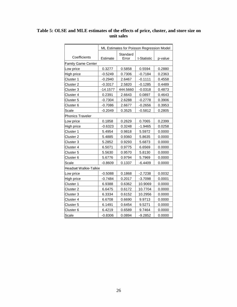
We maximize this function with respect to the parameters ak, bi and c, and obtain the

estimates given in table 5. For each product, the ‘low price’ and the ‘high price’

coefficients are the estimates of log(bi) at the lower and the higher price-points

respectively setting a value of 0 for the middle price-point. The next six coefficient

estimates give the values of log(ak) for the six clusters. The last estimate gives the value

of c, the exponent of xkit.

We find that bi decreases with price for the family game center and the phonics

traveler. The amount of decrease is statistically significant at 95% confidence level for

the phonics traveler, but not for the family game center. Thus, hypothesis H1 is validated

for the phonics traveler but not for the family game center. The lack of significance may

be because the quantity of sales registered at each price-point for this product is too small

for statistical analysis.

For the headset walkie-talkie, we find that hypothesis H2 is validated with a 99%

confidence level. To understand the reasons for this behavior, we discussed the results

with the managers of the subject firm and several other retailing firms. The following

explanations emerged from our discussions:

18

1. Price as an indicator of quality: The headset walkie-talkie is a complex electronic

item. The consumers find it difficult to judge its quality, and therefore, use price as an

indicator of quality. The managers used wine as another example where consumers might

be expected to use price as an indicator of quality. This argument did not apply to the

family game center because it is a board game, and easily understood by the customer, so

that price need not be used as an indicator of quality. It also did not apply to the phonics

traveler because it is a branded item.

This explanation is similar to those given by Gerstner (1985), Lichtenstein and

Burton (1989), Tellis and Wernerfelt (1987) and Zeithaml (1988) for consumers using

price as an indicator of quality. However, our finding is distinct from these articles

because these articles compare price and quality across products in a category while we

document the increase in sales with price for the same product due to a likely increase in

quality perception.

2. Sweet spot of pricing: The price-point $19.99 is more popular for gift purchases

than $14.99. Consumers may like the headset walkie-talkie as a gift item, so that the unit

sales at $19.99 exceed those at $14.99.

We now fit demand curves to the two products with downward sloping demand,

the family game center and the phonics traveler, to estimate the price elasticity of demand

and find the price that maximizes profit. We assume that the mean demand depends on

price according to a constant elasticity demand curve. We then modify the Poisson

regression model presented above to estimate this demand curve. The mean demand for

the store in cluster k at the price-point i in week t is given by

ckit k ki kita P xhl = ,

19

where kpP is the i-th price-point in cluster k, h is the price elasticity of demand, and the

other variables have the same definition as before. The log likelihood function is given by

( ) ( )kit kit k kit kit kitk i t

L y a P c x yé ù= - l + + h + -ê úë ûå, ,

log log log log log ! .

We maximize this function with respect to ak, h and c. The price elasticity of demand for

the phonics traveler is found to be –2.02 with a standard error of 0.90 and a p-value of

0.01. For the family game center, it is found to be –1.95 with a standard error of 1.64 and

a p-value of 0.12. Again, the lower significance level for the family game center may be

because it is a very slow-moving item with a few units sold at each price.

The optimal price is found by maximizing the expected profit function,

( )constant ,ki kit kit ki kiE P C P CP+ h hp = l - l = ´ -1[ ]

where C denotes unit cost. The optimal price is found to be kiP C= h + h/ (1 ) . It is

equal to $35.65 for the phonics traveler for a cost of $18 and a profit margin of $17.65.

For the family game center, it is equal to $22.58 for a cost of $11 and a profit margin of

$11.58. Thus, the price for the phonics traveler is found to be higher than the existing

price of $29.99 and the price for the family game center is found to be lower than the

existing price of $24.99 at this retail chain. The increase in expected gross profit from

moving to the optimal price is 3.8% for the phonics traveler and 0.9% for the family

game center.

5. Conclusions

We have presented a methodology for conducting experiments in a retail store that can

help retailing managers learn more about their consumers. This methodology is useful not

just for finding consumer reactions to different price-points, but also to test the effects of

20

different types of assortments, and store-push levers such as ‘item of the week

promotion’, large shelf-space display, and salesperson push. The critical aspect of the

methodology is the selection of stores for the experiment. We have shown how the

differences between stores may be defined using their sales characteristics and used to

partition stores into a randomized block design. This technique is advantageous because

an experiment with a small number of experimental stores may yield accurate results

applicable to the entire chain.

Our results show that the relationship between price and demand need not be

downward sloping and depends on the characteristics of a product. This result brings out

the importance of experimentation in a store. It also has implications for further research

to explain how consumers react to prices and how prices are set in a store.

References

Baker, J., M. Levy and D. Grewal (1992), An experimental approach to making retail

store environmental decisions, Journal of Retailing, 68(4), 445-460.

Brodie, R. and C. Kluyver (1984), Attraction Versus Linear and Multiplicative Market

Share Models: An Empirical Evaluation, Journal of Marketing Research, 21, 194-

201.

Cooper, L. G. (1993), Market Share Models, Chapter 6 in Handbooks in OR & MS. Vol.

5. Marketing, J. Eliashberg and G. L. Lilien, eds., 259-314.

Curhan R. (1974), The Effects of Merchandising and Temporary Promotional Activities

on the Sales of Fresh Fruits and Vegetables in Supermarkets, Journal of

Marketing Research, 11(3), 286-294.

21

Etgar, M. and N. Malhotra (1981), Determinants of Price Dependency: Personal and

Perceptual Factors, Journal of Consumer Research, 8(2), 217-222.

Fisher, M. L. and K. Rajaram (2000) Accurate Retail Testing of Fashion Merchandise:

Methodology and Application, Marketing Science, 19(3), 266-278.

Gagnon, J. P. and J. T. Osterhaus (1985), Effectiveness of Floor Displays on the Sales of

Retail Products, Journal of Retailing, 61(1), 104-116.

Gerstner, E. (1985), Do Higher Prices Signal Higher Quality? Journal of Marketing

Research, 22, 209-15.

Ghosh, A., S. Neslin and R. Shoemaker (1984), A Comparison of Market Share Models

and Estimation Procedures, Journal of Marketing Research, 21, 202-210.

Ghosh, S. and C. R. Rao (eds.) (1996), Design and Analysis of Experiments, Handbook of

Statistics, Vol 13, Elsevier Science, Amsterdam.

Green, W. H. (1997), Econometric Analysis, 3rd ed., Prentice Hall, New Jersey.

Lichtenstein, D. R. and S. Burton (1989), The Relationship Between Perceived Quality

and Objective Price-Quality, Journal of Marketing Research, 26, 429-443.

Mason, R., R. Gunst, and J. Hess (1989), Statistical Design and Analysis of Experiments,

John Wiley & Sons, New York.

Montgomery, D. (1991), Design and Analysis of Experiments, 3rd ed., John Wiley &

Sons, New York.

Narasimhan, C., S. A. Neslin, and S. K. Sen (1996), Promotional elasticities and category

characteristics, Journal of Marketing, 60(2), 17-30.

Naert, Ph. and M. Weverbergh (1981), On the Prediction Power of Market Share

Attraction Models, Journal of Marketing Research, 21, 202-210.

22

Nemhauser, G. and L. Wolsey (1988), Integer and Combinatorial Optimization, John

Wiley & Sons, New York.

Neslin, S. and R. Shoemaker (1983), Using a Natural Experiment to Estimate Price

Elasticity: The 1974 Sugar Shortage and the Ready-to-Eat Cereal Market, Journal

of Marketing, 47(1), 44-57.

Nevin, J. (1974), Laboratory Experiments for Estimating Consumer Demand: A

Validation Study, Journal of Marketing Research, 9, 261-268.

Rao, V. R. (1993), Pricing Models in Marketing, Chapter 11 in Handbooks in OR & MS.

Vol. 5. Marketing, J. Eliashberg and G. L. Lilien, eds., p.517-552.

Tellis, G. J. (1988), The Price Elasticity of Selective Demand: A Meta-Analysis of

Econometric Models of Sales, Journal of Marketing Research, 25, 331-341.

Tellis, G. J. and B. Wernerfelt (1987), “Competitive Price and Quality Under Assymetric

Information,” Marketing Science, 6(3), 240-253.

Zeithaml V. (1988), Consumer Perceptions of Price, Quality and Value: A Means-End

Model and Synthesis of Evidence, Journal of Marketing, 52, 2-22.

23

Table 1: Summary of the stores used in the experiment classified into cluster

% Sales from each category Cluster Store Opening Year

Year To Date Sales ($ '000) 1 2 3 4 5

102 92 680.8 12.1 5.7 8.4 8.0 8.3 204 94 514.1 12.4 4.6 7.8 9.4 8.9

1

103 93 610.5 11.2 5.2 8.8 8.5 8.2 108 96 481.7 9.7 12.0 7.3 9.9 10.6 402 94 477.9 8.7 15.2 6.7 9.6 9.8

2

105 94 492.2 8.1 12.3 6.1 9.9 9.6 302 94 432.6 9.6 6.0 8.4 10.2 8.6 303 95 434.1 10.7 6.3 7.8 11.4 8.2

3

205 95 466.2 10.6 5.7 7.7 10.3 9.7 325 96 561.8 10.7 6.0 7.7 8.6 9.2 526 96 556.1 10.9 6.5 8.3 8.6 9.9

4

401 94 644.1 11.1 6.7 7.3 7.6 8.6 107 94 523.5 10.2 4.3 6.1 11.2 12.0 527 96 441.8 11.1 5.8 6.1 11.1 13.2

5

326 96 438.1 10.3 5.3 7.3 10.5 12.6 110 95 595.8 11.5 9.0 7.5 8.2 7.3 504 96 553.3 12.3 9.4 8.3 8.9 6.3

6

503 96 547 12.9 9.9 7.8 8.6 6.3

Table 2: Summary of products and price-points used in the experiment

Prices ($)

Low Medium (Existing list price)

High Purchase Cost

($)

A: Family Game Center 19.99 24.99 29.99 11 B: Phonics Traveler 24.99 29.99 34.99 18 C: Headset Walkie-Talkie 14.99 19.99 24.99 11

24

Table 3: Experiment layout showing the random assignment of stores in each cluster to price-points for each product

(a) Family Game Center

Prices ($) Clusters 19.99 24.99 29.99

1 204 103 102 2 108 105 402 3 302 205 303 4 325 401 526 5 107 326 527 6 504 503 110

(b) Phonics Traveler

Prices ($) Clusters 24.99 29.99 34.99

1 102 103 204 2 108 105 402 3 303 205 302 4 526 401 325 5 107 326 527 6 504 503 110

(c) Headset Walkie-Talkie

Prices ($) Clusters 14.99 19.99 24.99

1 102 103 204 2 108 105 402 3 303 205 302 4 325 401 526 5 527 326 107 6 504 503 110

25

Table 4: Total sales recorded for each product in each store

Family Game Center Phonics Traveler Headset Walkie Talkie

Cluster Store Price Total Unit

Sales Price Total Unit

Sales Price Total Unit

Sales

Average number of transactions

per week102 29.99 0 24.99 6 14.99 15 1954.83204 19.99 2 34.99 0 24.99 5 1780.67

1

103 24.99 1 29.99 3 19.99 16 1741.50108 19.99 2 24.99 3 14.99 8 1485.33402 29.99 0 34.99 6 24.99 6 1355.50

2

105 24.99 1 29.99 2 19.99 18 1714.00302 19.99 0 34.99 2 24.99 12 1294.17303 29.99 0 24.99 6 14.99 4 1263.33

3

205 24.99 0 29.99 2 19.99 10 1343.00325 19.99 2 34.99 0 14.99 9 1911.33526 29.99 0 24.99 12 24.99 6 1872.17

4

401 24.99 3 29.99 10 19.99 9 1916.67107 19.99 1 24.99 5 24.99 5 1795.00527 29.99 1 34.99 1 14.99 6 1266.17

5

326 24.99 0 29.99 5 19.99 8 1328.33110 29.99 2 34.99 6 24.99 2 1694.33504 19.99 0 24.99 1 14.99 5 1424.67

6

503 24.99 0 29.99 4 19.99 13 2019.17 19.99 7 24.99 33 14.99 47 24.99 5 29.99 26 19.99 74

Total Sales

29.99 3 34.99 15 24.99 36

26

Table 5: OLSE and MLE estimates of the effects of price, cluster, and store size on unit sales

ML Estimates for Poisson Regression Model

Coefficients Estimate Standard

Error t-Statistic p-value Family Game Center Low price 0.3277 0.5858 0.5594 0.2880 High price -0.5249 0.7306 -0.7184 0.2363 Cluster 1 -0.2940 2.6467 -0.1111 0.4558 Cluster 2 -0.3317 2.5820 -0.1285 0.4489 Cluster 3 -14.1577 444.5660 -0.0318 0.4873 Cluster 4 0.2391 2.6643 0.0897 0.4643 Cluster 5 -0.7304 2.6288 -0.2778 0.3906 Cluster 6 -0.7086 2.6677 -0.2656 0.3953 Scale -0.2049 0.3525 -0.5812 0.2805 Phonics Traveler Low price 0.1858 0.2629 0.7065 0.2399 High price -0.6323 0.3248 -1.9465 0.0258 Cluster 1 5.4954 0.9818 5.5972 0.0000 Cluster 2 5.4885 0.9360 5.8635 0.0000 Cluster 3 5.2852 0.9293 5.6873 0.0000 Cluster 4 6.5071 0.9775 6.6569 0.0000 Cluster 5 5.5630 0.9570 5.8130 0.0000 Cluster 6 5.6776 0.9794 5.7969 0.0000 Scale -0.8609 0.1337 -6.4409 0.0000 Headset Walkie-Talkie Low price -0.5088 0.1868 -2.7238 0.0032 High price -0.7484 0.2017 -3.7098 0.0001 Cluster 1 6.9388 0.6362 10.9069 0.0000 Cluster 2 6.6475 0.6172 10.7704 0.0000 Cluster 3 6.3334 0.6152 10.2956 0.0000 Cluster 4 6.6708 0.6690 9.9713 0.0000 Cluster 5 6.1491 0.6454 9.5271 0.0000 Cluster 6 6.4219 0.6589 9.7464 0.0000 Scale -0.8306 0.0894 -9.2852 0.0000

27

Figure 1: Plot of total sales of each product at each price-point showing how demand varies with price

0

10

20

30

40

50

60

70

80

Low Medium High

Price

Unit Sales

Family Game CenterPhonics TravelerHeadset Walkie Talkie