In te format provided b te autors and unedited. Distance ... · still be a key variable in the fitting procedure. The distance between the electrons of Gd and the bound The distance

In the format provided by the authors and unedited.

1

Distance-dependent Magnetic Resonance Tuning as a

Versatile MRI Sensing Platform for Biological Targets

Jin-sil Choi1,2,3†, Soojin Kim1,2,3†, Dongwon Yoo1,2, Tae-Hyun Shin1,2,3, Hoyoung Kim1,2,3, Muller D. Gomes4,5, Sun Hee Kim6, Alexander Pines4,5, and Jinwoo Cheon1,2,3*

1Center for Nanomedicine, Institute for Basic Science (IBS), Seoul 03722, Republic of Korea 2Yonsei-IBS Institute, Yonsei University, Seoul 03722, Republic of Korea

3Department of Chemistry, Yonsei University, Seoul 03722, Republic of Korea 4Department of Chemistry, University of California, Berkeley, California 94720

5Materials Sciences Division, Lawrence Berkeley National Laboratory, Berkeley, California 94720 6Western Seoul Center, Korea Basic Science Institute, Seoul 03760, Republic of Korea

†These authors contributed equally to this work.

*e-mail: [email protected]

Distance-dependent magnetic resonance tuning as a versatile MRI sensing platform for

biological targets

© 2017 Macmillan Publishers Limited, part of Springer Nature. All rights reserved.

SUPPLEMENTARY INFORMATIONDOI: 10.1038/NMAT4846

NATURE MATERIALS | www.nature.com/naturematerials 1

http://dx.doi.org/10.1038/nmat4846

2

Supplementary Figures and Table

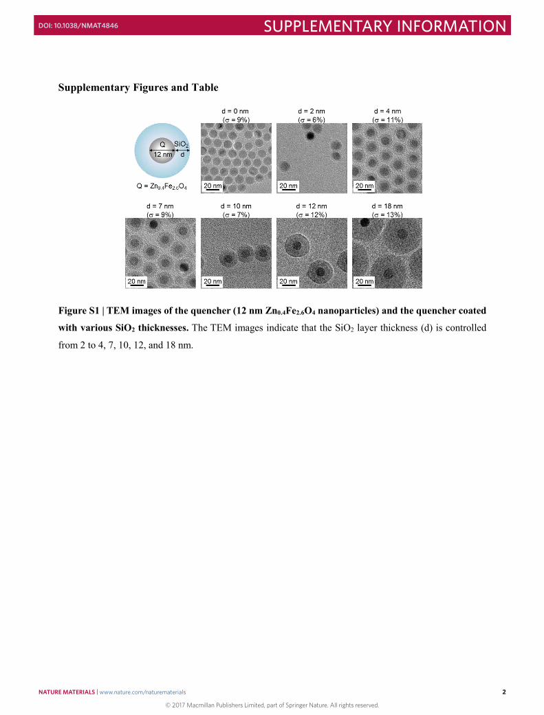
Figure S1 | TEM images of the quencher (12 nm Zn0.4Fe2.6O4 nanoparticles) and the quencher coated

with various SiO2 thicknesses. The TEM images indicate that the SiO2 layer thickness (d) is controlled

from 2 to 4, 7, 10, 12, and 18 nm.





3

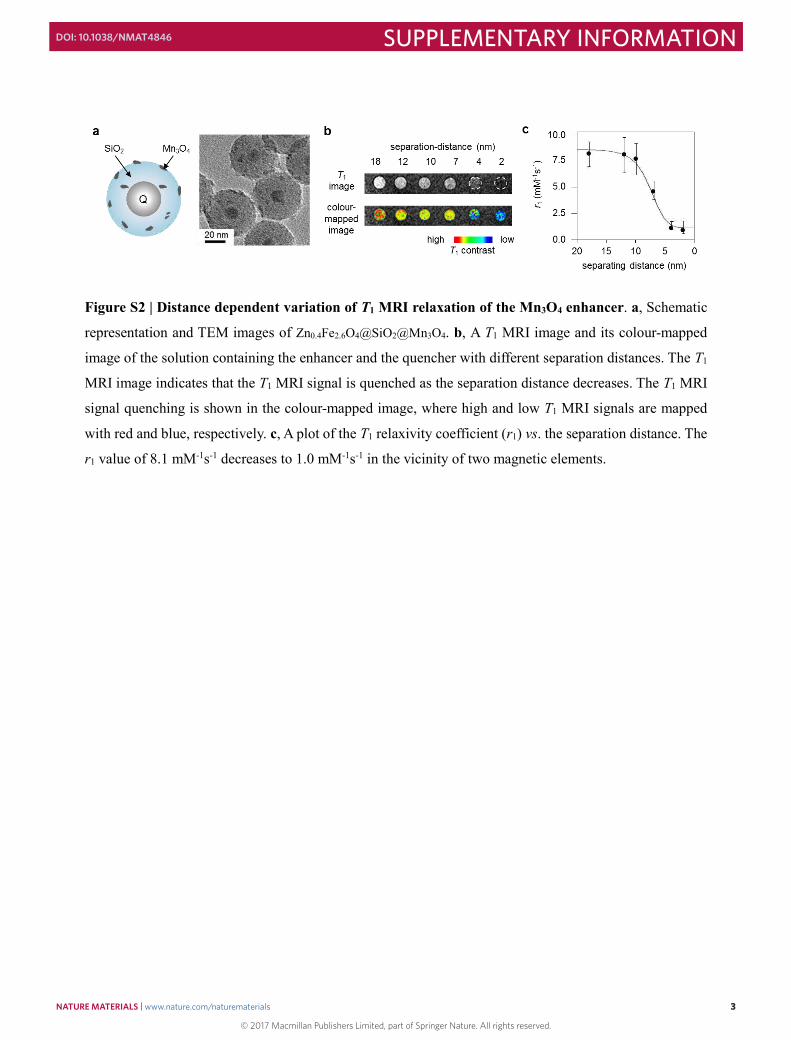
Figure S2 | Distance dependent variation of T1 MRI relaxation of the Mn3O4 enhancer. a, Schematic

representation and TEM images of Zn0.4Fe2.6O4@SiO2@Mn3O4. b, A T1 MRI image and its colour-mapped

image of the solution containing the enhancer and the quencher with different separation distances. The T1

MRI image indicates that the T1 MRI signal is quenched as the separation distance decreases. The T1 MRI

signal quenching is shown in the colour-mapped image, where high and low T1 MRI signals are mapped

with red and blue, respectively. c, A plot of the T1 relaxivity coefficient (r1) vs. the separation distance. The

r1 value of 8.1 mM-1s-1 decreases to 1.0 mM-1s-1 in the vicinity of two magnetic elements.





4

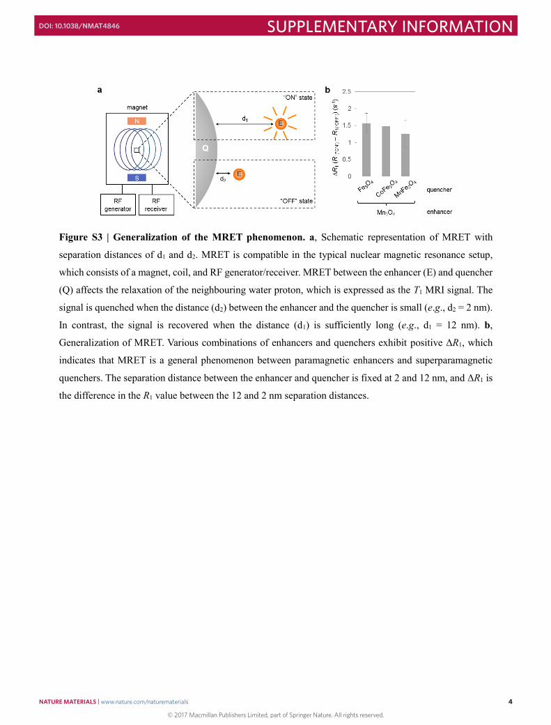
Figure S3 | Generalization of the MRET phenomenon. a, Schematic representation of MRET with

separation distances of d1 and d2. MRET is compatible in the typical nuclear magnetic resonance setup,

which consists of a magnet, coil, and RF generator/receiver. MRET between the enhancer (E) and quencher

(Q) affects the relaxation of the neighbouring water proton, which is expressed as the T1 MRI signal. The

signal is quenched when the distance (d2) between the enhancer and the quencher is small (e.g., d2 = 2 nm).

In contrast, the signal is recovered when the distance (d1) is sufficiently long (e.g., d1 = 12 nm). b,

Generalization of MRET. Various combinations of enhancers and quenchers exhibit positive ΔR1, which

indicates that MRET is a general phenomenon between paramagnetic enhancers and superparamagnetic

quenchers. The separation distance between the enhancer and quencher is fixed at 2 and 12 nm, and ΔR1 is

the difference in the R1 value between the 12 and 2 nm separation distances.





5

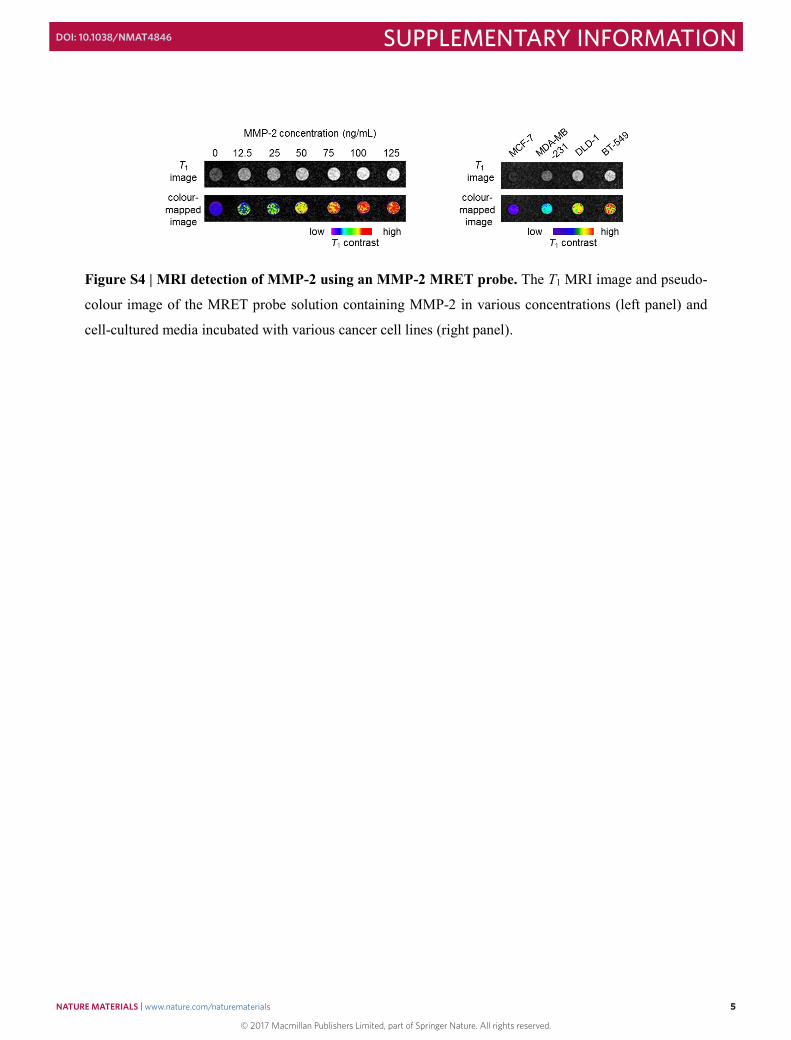
Figure S4 | MRI detection of MMP-2 using an MMP-2 MRET probe. The T1 MRI image and pseudo-

colour image of the MRET probe solution containing MMP-2 in various concentrations (left panel) and

cell-cultured media incubated with various cancer cell lines (right panel).





6

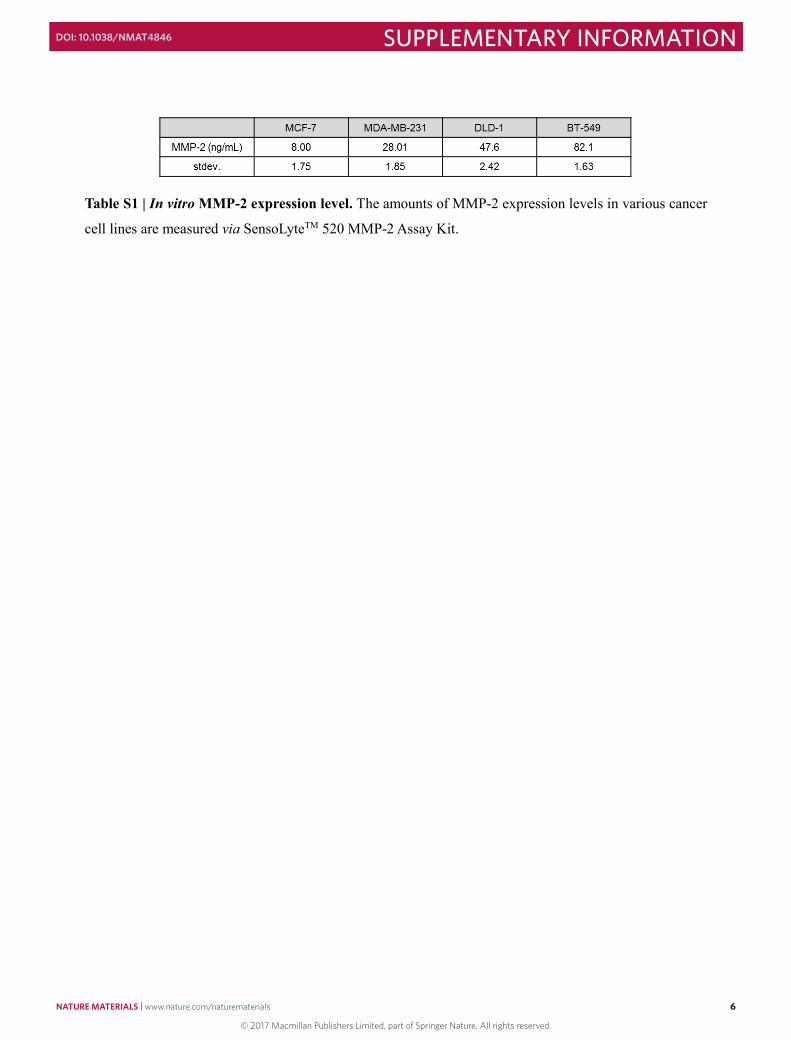
Table S1 | In vitro MMP-2 expression level. The amounts of MMP-2 expression levels in various cancer

cell lines are measured via SensoLyteTM 520 MMP-2 Assay Kit.





7

Supplementary Note 1. Calculation of the room temperature T1e.

The r1 values for the 2, 7, and 12 nm separation distances were measured at the following fields: 3, 9.4, and

15.2 T (Fig. 2d). Two changes in the dynamics are needed to explain the change in the T1 MRI signal as a

function of the separation distance: an increase in the electron relaxation time (T1e) and the water exchange

time (τm) as the separation distance decreases.

The r1 at various frequencies was fitted to the following model with three correlation times. The most

important is T1e because it is the shortest. The T1e of the Gd-DOTA tends to be in the nanoseconds regime

at room temperature1. The next shortest correlation time is the rotational correlation time (τr) of the Gd-

DOTA. Although τr of Gd-DOTA is typically hundreds of picoseconds, τr for the MRET phenomenon

becomes slow because Gd-DOTA is attached to a nanoparticle. By using the Stokes equation τr is estimated

to be approximately within the microsecond regime, which is too slow to contribute to relaxation2,3. It is

important to note that τr could vary up to the nanosecond range depending on the flexibility of the linkers

and/or type of nanoparticles4,5. The last correlation time is τm. Although τm is likely to be the slowest, it can

still contribute to the T1 MRI signal by affecting how the bound water exchanges with bulk water. Therefore,

even if τm has no impact on the shape of the spectral density function that governs the T1 MRI signal, it can

still be a key variable in the fitting procedure. The distance between the electrons of Gd and the bound

water protons is fixed at 3.05 Angstroms which is an estimate based on other Lanthanide water complexes6.

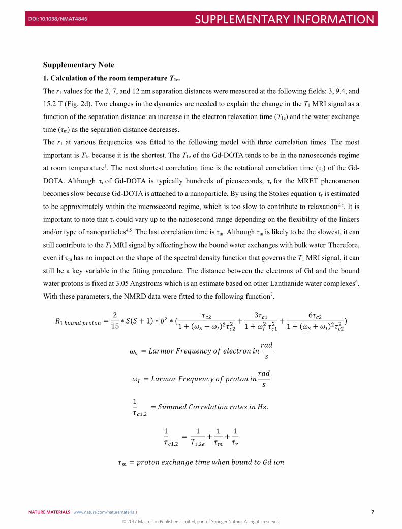
With these parameters, the NMRD data were fitted to the following function7.

𝑅𝑅1 𝑏𝑏𝑏𝑏𝑏𝑏𝑏𝑏𝑏𝑏 𝑝𝑝𝑝𝑝𝑏𝑏𝑝𝑝𝑏𝑏𝑏𝑏 = 215 ∗ 𝑆𝑆(𝑆𝑆 + 1) ∗ 𝑏𝑏2 ∗ ( 𝜏𝜏𝑐𝑐2

1 + (𝜔𝜔𝑆𝑆 − 𝜔𝜔𝐼𝐼)2𝜏𝜏𝑐𝑐22 + 3𝜏𝜏𝑐𝑐1

1 + 𝜔𝜔𝐼𝐼2 𝜏𝜏𝑐𝑐1

2 + 6𝜏𝜏𝑐𝑐21 + (𝜔𝜔𝑆𝑆 + 𝜔𝜔𝐼𝐼)2𝜏𝜏𝑐𝑐2

2 )

𝜔𝜔𝑠𝑠 = 𝐿𝐿𝐿𝐿𝐿𝐿𝐿𝐿𝐿𝐿𝐿𝐿 𝐹𝐹𝐿𝐿𝐹𝐹𝐹𝐹𝐹𝐹𝐹𝐹𝐹𝐹𝐹𝐹𝐹𝐹 𝐿𝐿𝑜𝑜 𝐹𝐹𝑒𝑒𝐹𝐹𝐹𝐹𝑒𝑒𝐿𝐿𝐿𝐿𝐹𝐹 𝑖𝑖𝐹𝐹 𝐿𝐿𝐿𝐿𝑟𝑟𝑠𝑠

𝜔𝜔𝐼𝐼 = 𝐿𝐿𝐿𝐿𝐿𝐿𝐿𝐿𝐿𝐿𝐿𝐿 𝐹𝐹𝐿𝐿𝐹𝐹𝐹𝐹𝐹𝐹𝐹𝐹𝐹𝐹𝐹𝐹𝐹𝐹 𝐿𝐿𝑜𝑜 𝑝𝑝𝐿𝐿𝐿𝐿𝑒𝑒𝐿𝐿𝐹𝐹 𝑖𝑖𝐹𝐹 𝐿𝐿𝐿𝐿𝑟𝑟𝑠𝑠

1𝜏𝜏𝑐𝑐1,2

= 𝑆𝑆𝐹𝐹𝐿𝐿𝐿𝐿𝐹𝐹𝑟𝑟 𝐶𝐶𝐿𝐿𝐿𝐿𝐿𝐿𝐹𝐹𝑒𝑒𝐿𝐿𝑒𝑒𝑖𝑖𝐿𝐿𝐹𝐹 𝐿𝐿𝐿𝐿𝑒𝑒𝐹𝐹𝑠𝑠 𝑖𝑖𝐹𝐹 𝐻𝐻𝐻𝐻.

1𝜏𝜏𝑐𝑐1,2

= 1𝑇𝑇1,2𝑒𝑒

+ 1𝜏𝜏𝑚𝑚

+ 1𝜏𝜏𝑝𝑝

𝜏𝜏𝑚𝑚 = 𝑝𝑝𝐿𝐿𝐿𝐿𝑒𝑒𝐿𝐿𝐹𝐹 𝐹𝐹𝑒𝑒𝐹𝐹ℎ𝐿𝐿𝐹𝐹𝑎𝑎𝐹𝐹 𝑒𝑒𝑖𝑖𝐿𝐿𝐹𝐹 𝑤𝑤ℎ𝐹𝐹𝐹𝐹 𝑏𝑏𝐿𝐿𝐹𝐹𝐹𝐹𝑟𝑟 𝑒𝑒𝐿𝐿 𝐺𝐺𝑟𝑟 𝑖𝑖𝐿𝐿𝐹𝐹





8

𝜏𝜏𝑟𝑟 = 𝑝𝑝𝑝𝑝𝑝𝑝𝑝𝑝𝑝𝑝𝑝𝑝 𝑝𝑝𝑝𝑝𝑝𝑝𝑟𝑟𝑝𝑝𝑟𝑟𝑝𝑝𝑝𝑝𝑟𝑟𝑟𝑟 𝑐𝑐𝑝𝑝𝑝𝑝𝑝𝑝𝑐𝑐𝑟𝑟𝑟𝑟𝑝𝑝𝑟𝑟𝑝𝑝𝑝𝑝 𝑝𝑝𝑟𝑟𝑡𝑡𝑐𝑐 𝑤𝑤ℎ𝑐𝑐𝑝𝑝 𝑏𝑏𝑝𝑝𝑏𝑏𝑝𝑝𝑏𝑏 𝑝𝑝𝑝𝑝 𝐺𝐺𝑏𝑏 𝑟𝑟𝑝𝑝𝑝𝑝

1𝑇𝑇1,𝑏𝑏𝑏𝑏𝑏𝑏𝑏𝑏 𝑝𝑝𝑟𝑟𝑝𝑝𝑝𝑝𝑝𝑝𝑝𝑝

= 𝑝𝑝𝑚𝑚𝜏𝜏𝑚𝑚 + 𝑇𝑇1,𝑏𝑏𝑝𝑝𝑏𝑏𝑝𝑝𝑏𝑏 𝑝𝑝𝑟𝑟𝑝𝑝𝑝𝑝𝑝𝑝𝑝𝑝

All fitting was performed with the nonlinear least square fitting software provided by MATLAB (code

below). Multiple initial guesses were used for the least squares fitting, preventing the least squares

algorithm from getting stuck in a local minimum. The answer with the smallest residual was selected.

The following results were obtained from this fitting procedure. Both T1e and τm decreases as the separation

distance increases. T1e changes dramatically from 135.1 to 15.5 ns, and τm changes from 95.5 to 9.7 s.

Thickness (nm) τm (µs) T1e (ns) Residuals

2 95.5 135.1 1.51 x 10-4

7 19.5 29.7 6.18 x 10-6

12 9.7 15.5 1.03 x 10-2

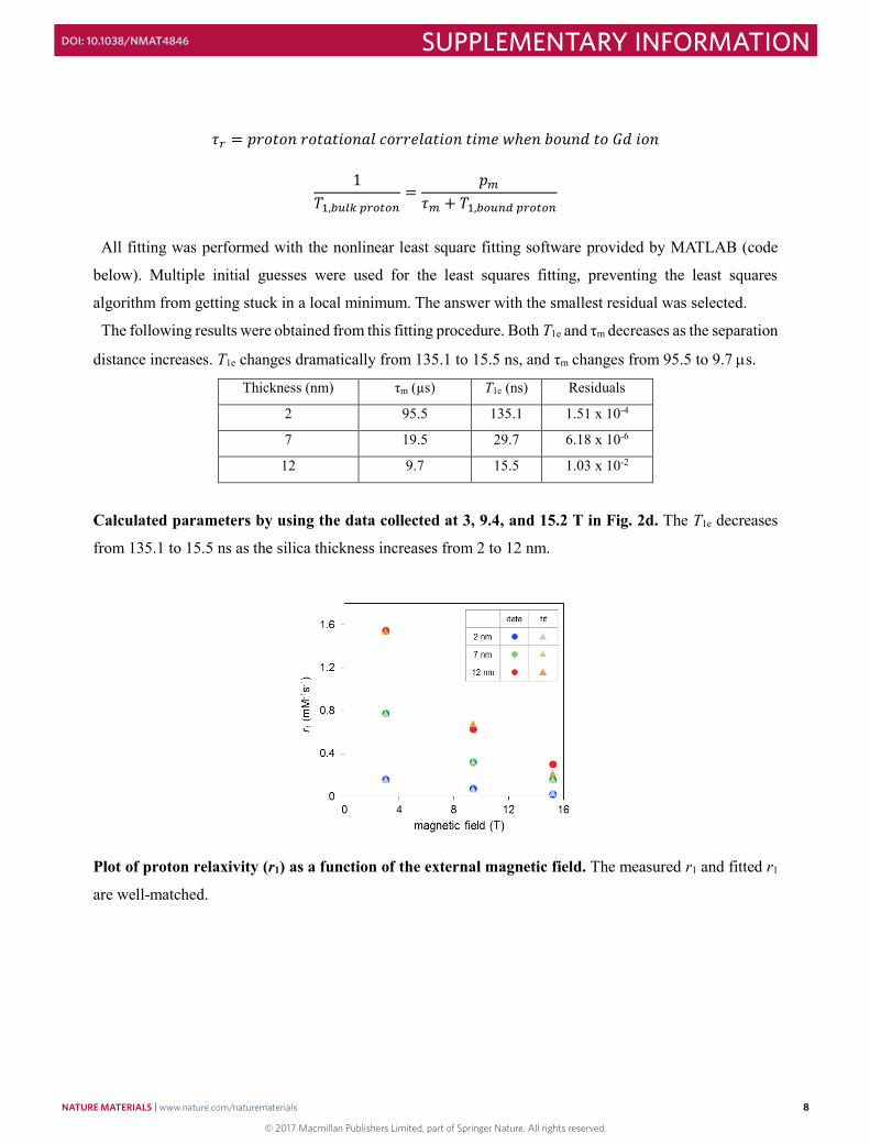
Calculated parameters by using the data collected at 3, 9.4, and 15.2 T in Fig. 2d. The T1e decreases

from 135.1 to 15.5 ns as the silica thickness increases from 2 to 12 nm.

Plot of proton relaxivity (r1) as a function of the external magnetic field. The measured r1 and fitted r1

are well-matched.





9

2. Spectral density of the enhancer

To better understand how T1e affects the T1 MRI signal, one can examine the spectral density function of

the interaction between Gd-DOTA and bound water. From the NMRD profiles, T1e is known and is used to

calculate the spectral density at each field.

Spectral density of the Gd-DOTA enhancer. a,b, The spectral density significantly shifts from broad to

narrow (a), and the intensity of the enhancer spectral density decreases at the proton Larmor frequency of

128 MHz (b) as the separation distance decreases.

The increase in T1e significantly shifts the spectral density of the enhancer from broad to narrow when the

separation distance decreases from 12 to 2 nm (Fig. a). It is necessary to zoom into the studied field range

to understand how T1e affects the T1 MRI signal. The magnified figure indicates that the intensity of the

enhancer spectral density at 128 MHz is largely reduced, which can result in a decrease in the T1 MRI signal

(Fig. b).





10

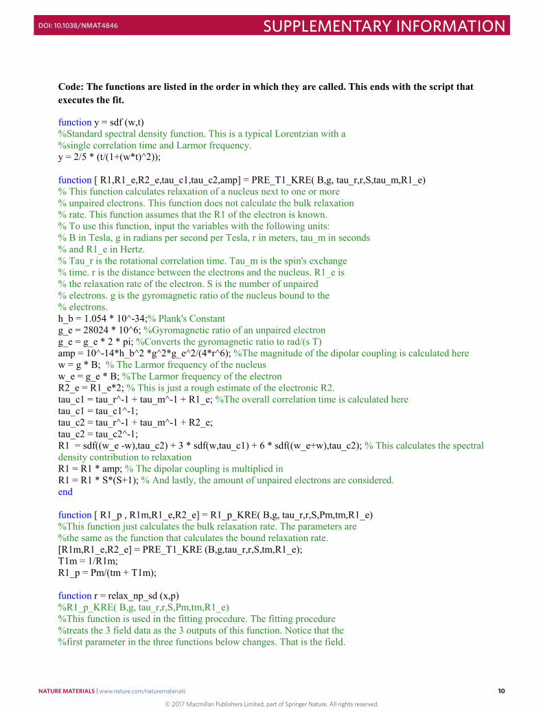
Code: The functions are listed in the order in which they are called. This ends with the script that executes the fit.

function y = sdf (w,t) %Standard spectral density function. This is a typical Lorentzian with a %single correlation time and Larmor frequency. y = 2/5 * (t/(1+(w*t)^2)); function [ R1,R1_e,R2_e,tau_c1,tau_c2,amp] = PRE_T1_KRE( B,g, tau_r,r,S,tau_m,R1_e) % This function calculates relaxation of a nucleus next to one or more % unpaired electrons. This function does not calculate the bulk relaxation % rate. This function assumes that the R1 of the electron is known. % To use this function, input the variables with the following units: % B in Tesla, g in radians per second per Tesla, r in meters, tau_m in seconds % and R1_e in Hertz. % Tau_r is the rotational correlation time. Tau_m is the spin's exchange % time. r is the distance between the electrons and the nucleus. R1_e is % the relaxation rate of the electron. S is the number of unpaired % electrons. g is the gyromagnetic ratio of the nucleus bound to the % electrons. h_b = 1.054 * 10^-34;% Plank's Constant g_e = 28024 * 10^6; %Gyromagnetic ratio of an unpaired electron g_e = g_e * 2 * pi; %Converts the gyromagnetic ratio to rad/(s T) amp = 10^-14*h_b^2 *g^2*g_e^2/(4*r^6); %The magnitude of the dipolar coupling is calculated here w = g * B; % The Larmor frequency of the nucleus w_e = g_e * B; %The Larmor frequency of the electron R2_e = R1_e*2; % This is just a rough estimate of the electronic R2. tau_c1 = tau_r^-1 + tau_m^-1 + R1_e; %The overall correlation time is calculated here tau_c1 = tau_c1^-1; tau_c2 = tau_r^-1 + tau_m^-1 + R2_e; tau_c2 = tau_c2^-1; R1 = sdf((w_e -w),tau_c2) + 3 * sdf(w,tau_c1) + 6 * sdf((w_e+w),tau_c2); % This calculates the spectral density contribution to relaxation R1 = R1 * amp; % The dipolar coupling is multiplied in R1 = R1 * S*(S+1); % And lastly, the amount of unpaired electrons are considered. end function [ R1_p , R1m,R1_e,R2_e] = R1_p_KRE( B,g, tau_r,r,S,Pm,tm,R1_e) %This function just calculates the bulk relaxation rate. The parameters are %the same as the function that calculates the bound relaxation rate. [R1m,R1_e,R2_e] = PRE_T1_KRE (B,g,tau_r,r,S,tm,R1_e); T1m = 1/R1m; R1_p = Pm/(tm + T1m); function r = relax_np_sd (x,p) %R1_p_KRE( B,g, tau_r,r,S,Pm,tm,R1_e) %This function is used in the fitting procedure. The fitting procedure %treats the 3 field data as the 3 outputs of this function. Notice that the %first parameter in the three functions below changes. That is the field.





11

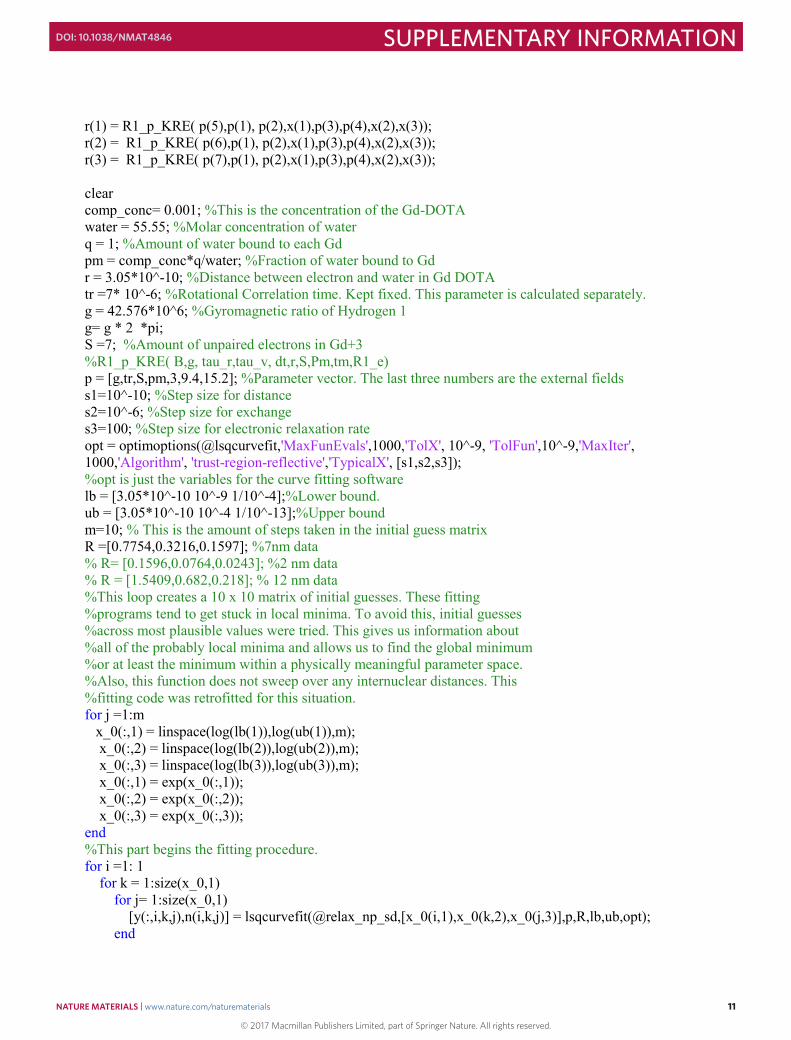
r(1) = R1_p_KRE( p(5),p(1), p(2),x(1),p(3),p(4),x(2),x(3)); r(2) = R1_p_KRE( p(6),p(1), p(2),x(1),p(3),p(4),x(2),x(3)); r(3) = R1_p_KRE( p(7),p(1), p(2),x(1),p(3),p(4),x(2),x(3)); clear comp_conc= 0.001; %This is the concentration of the Gd-DOTA water = 55.55; %Molar concentration of water q = 1; %Amount of water bound to each Gd pm = comp_conc*q/water; %Fraction of water bound to Gd r = 3.05*10^-10; %Distance between electron and water in Gd DOTA tr =7* 10^-6; %Rotational Correlation time. Kept fixed. This parameter is calculated separately. g = 42.576*10^6; %Gyromagnetic ratio of Hydrogen 1 g= g * 2 *pi; S =7; %Amount of unpaired electrons in Gd+3 %R1_p_KRE( B,g, tau_r,tau_v, dt,r,S,Pm,tm,R1_e) p = [g,tr,S,pm,3,9.4,15.2]; %Parameter vector. The last three numbers are the external fields s1=10^-10; %Step size for distance s2=10^-6; %Step size for exchange s3=100; %Step size for electronic relaxation rate opt = optimoptions(@lsqcurvefit,'MaxFunEvals',1000,'TolX', 10^-9, 'TolFun',10^-9,'MaxIter', 1000,'Algorithm', 'trust-region-reflective','TypicalX', [s1,s2,s3]); %opt is just the variables for the curve fitting software lb = [3.05*10^-10 10^-9 1/10^-4];%Lower bound. ub = [3.05*10^-10 10^-4 1/10^-13];%Upper bound m=10; % This is the amount of steps taken in the initial guess matrix R =[0.7754,0.3216,0.1597]; %7nm data % R= [0.1596,0.0764,0.0243]; %2 nm data % R = [1.5409,0.682,0.218]; % 12 nm data %This loop creates a 10 x 10 matrix of initial guesses. These fitting %programs tend to get stuck in local minima. To avoid this, initial guesses %across most plausible values were tried. This gives us information about %all of the probably local minima and allows us to find the global minimum %or at least the minimum within a physically meaningful parameter space. %Also, this function does not sweep over any internuclear distances. This %fitting code was retrofitted for this situation. for j =1:m x_0(:,1) = linspace(log(lb(1)),log(ub(1)),m); x_0(:,2) = linspace(log(lb(2)),log(ub(2)),m); x_0(:,3) = linspace(log(lb(3)),log(ub(3)),m); x_0(:,1) = exp(x_0(:,1)); x_0(:,2) = exp(x_0(:,2)); x_0(:,3) = exp(x_0(:,3)); end %This part begins the fitting procedure. for i =1: 1 for k = 1:size(x_0,1) for j= 1:size(x_0,1) [y(:,i,k,j),n(i,k,j)] = lsqcurvefit(@relax_np_sd,[x_0(i,1),x_0(k,2),x_0(j,3)],p,R,lb,ub,opt); end





12

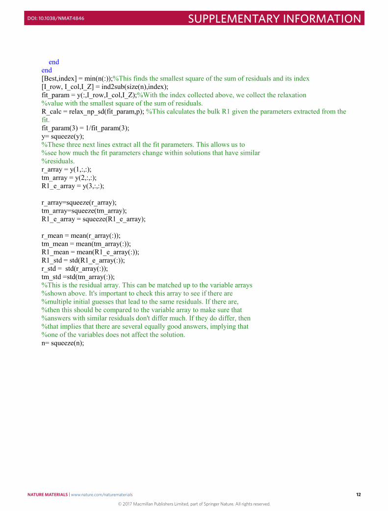
end end [Best,index] = min(n(:));%This finds the smallest square of the sum of residuals and its index [I_row, I_col,I_Z] = ind2sub(size(n),index); fit_param = y(:,I_row,I_col,I_Z);%With the index collected above, we collect the relaxation %value with the smallest square of the sum of residuals. R_calc = relax_np_sd(fit_param,p); %This calculates the bulk R1 given the parameters extracted from the fit. fit_param(3) = 1/fit_param(3); y= squeeze(y); %These three next lines extract all the fit parameters. This allows us to %see how much the fit parameters change within solutions that have similar %residuals. r_array = y(1,:,:); tm_array = y(2,:,:); R1_e_array = y(3,:,:); r_array=squeeze(r_array); tm_array=squeeze(tm_array); R1_e_array = squeeze(R1_e_array); r_mean = mean(r_array(:)); tm_mean = mean(tm_array(:)); R1_mean = mean(R1_e_array(:)); R1_std = std(R1_e_array(:)); r_std = std(r_array(:)); tm_std =std(tm_array(:)); %This is the residual array. This can be matched up to the variable arrays %shown above. It's important to check this array to see if there are %multiple initial guesses that lead to the same residuals. If there are, %then this should be compared to the variable array to make sure that %answers with similar residuals don't differ much. If they do differ, then %that implies that there are several equally good answers, implying that %one of the variables does not affect the solution. n= squeeze(n);





13

References 1. Atsarkin et al. Direct measurement of fast electron spin-lattice relaxation: Method and application to

nitroxide radical solutions and Gd3+ contrast agents. J. Phys. Chem. A 105, 9323-9327 (2001).

2. Ceccon, A., Tugarinov, V., Bax, A. & Clore, G. M. Global dynamics and exchange kinetics of a protein

on the surface of nanoparticles revealed by relaxation-based solution NMR spectroscopy. J. Am. Chem. Soc.

138, 5789-5792 (2016).

3. Zhang, B., Xie, M., Bruscheweiler-Li, L., Bingol, K. & Brüschweiler, R. Use of charged nanoparticles

in NMR-based metabolomics for spectral simplification and improved metabolite identification. Anal.

Chem. 87, 7211-7217 (2015).

4. Caravan, P. Strategies for increasing the sensitivity of gadolinium based MRI contrast agents. Chem. Soc.

Rev. 35, 512-523 (2006).

5. Floyd, W. C. et al. Conjugation effects of various linkers on Gd (III) MRI contrast agents with dendrimers:

optimizing the hydroxypyridinonate (HOPO) ligands with nontoxid, degradable esteramide (EA)

dendrimers for high relaxivity. J. Am. Chem. Soc. 133, 2390-2393 (2011).

6. Chemistry, B. Molecular Dynamics of Gd (III) Complexes in aqueous solution by HF EPR Alain Borel ,

Lothar Helm and Andre E . Merbach. 207-247 (2004).

7. Micskei, K., Helm, L., Brucher, E. & Merbach, A. E. Oxygen-17 NMR study of water exchange on

gadolinium polyaminopolyacetates [Gd(DTPA)(H2O)]2- and [Gd(DOTA)(H2O)]- related to NMR imaging.

Inorg. Chem. 32, 3844-3850 (1993).





Documents

In te format provided b te autors and unedited. Distance ... · still be a key variable in the fitting procedure. The distance between the electrons of Gd and the bound The distance