Quantifying the tension between the Higgs mass and ðg� 2Þ� in the constrained MSSM

Maria Eugenia Cabrera,1,* J. Alberto Casas,1,† Roberto Ruiz de Austri,2,‡ and Roberto Trotta3,x1Instituto de Fısica Teorica, IFT-UAM/CSIC, U.A.M., Cantoblanco, 28049 Madrid, Spain

2Instituto de Fısica Corpuscular, IFIC-UV/CSIC, Valencia, Spain3Astrophysics Group, Imperial College London, Blackett Laboratory, Prince Consort Rd, London SW7 2AZ, United Kingdom

(Received 19 January 2011; published 8 July 2011)

Supersymmetry has often been invoked as the new physics that might reconcile the experimental muon

magnetic anomaly, a�, with the theoretical prediction (basing the computation of the hadronic contri-

bution on eþe� data). However, in the context of the constrained minimal supersymmetric standard model

(CMSSM), the required supersymmetric contributions (which grow with decreasing supersymmetric

masses) are in potential tension with a possibly large Higgs mass (which requires large stop masses). In

the limit of very large mh supersymmetry gets decoupled, and the CMSSM must show the same

discrepancy as the standard model with a�. But it is much less clear for which size of mh does the

tension start to be unbearable. In this paper, we quantify this tension with the help of Bayesian techniques.

We find that for mh � 125 GeV the maximum level of discrepancy given the current data (� 3:2�) is

already achieved. Requiring less than 3� discrepancy, implies mh & 120 GeV. For a larger Higgs mass

we should give up either the CMSSM model or the computation of a� based on eþe�; or accept livingwith such an inconsistency.

DOI: 10.1103/PhysRevD.84.015006 PACS numbers: 13.40.Em, 12.60.Jv, 14.60.Ef, 14.80.Da

I. INTRODUCTION

The magnetic anomaly of the muon a� ¼ 12 ðg� 2Þ� has

been a classical and powerful test for new physics. As it isknown, the present experimental value and some of thetheoretical determinations of a� show a remarkable dis-

crepancy, suggesting physics beyond the standard model(SM) to account for it. However, the situation is stilluncertain, due essentially to inconsistencies between alter-native determinations of the contribution coming from thehadronic vacuum-polarization diagram, say �SM

hada�.

This contribution can be expressed in terms of the totalhadronic cross section eþe� ! had. Using direct experi-mental data for the latter, one obtains a final result for a�,

which is at more than 3� from the current experimentaldetermination [1], namely

�a� ¼ aexp� � aSM� ¼ 25:5� 8:0� 10�10 (1)

(the quoted error bars are 1�). This discrepancy has oftenbeen claimed as a signal of new physics. Obviously, if oneaccepts this point of view, the discrepancy should be curedby contributions from physics beyond the SM.

Admittedly, such claims are too strong. We are quiteaware of past experimental observables in apparent dis-agreement with the SM prediction, which have eventuallyconverged with it. This has occurred due to both experi-mental and theoretical subtleties that sometimes had notbeen fully understood or taken into account. As a matter of

fact, the experimental eþe� ! had cross section exhibitssome inconsistencies between different groups of experi-mental data. Using only BABAR data the discrepancyreduces to 2:4�, while without it the discrepancy becomes3:7�, [1]. The inconsistency is especially notorious if oneconsiders hadronic � decay data, which are theoreticallyrelated to the eþe� ! had cross section. Using just � datathe disagreement becomes 1:9�, [1], [2]. Although themore direct eþe� data are usually preferred to evaluateaSM� , these inconsistencies are warning us to be cautious

about the actual uncertainties involved in the determinationof aSM� .

If one takes the discrepancy between theory and experi-ment shown in Eq. (1) as a working hypothesis, one has toconsider possible candidates of new physics able to pro-vide the missing contribution to reproduce a

exp� . The mini-

mal supersymmetric standard model (MSSM) is then anatural option. We will consider here the simplest andmost extensively analyzed version of the MSSM, namely,the so-called constrained MSSM (CMSSM), in which thesoft parameters are assumed universal at a high scale (MX),where the supersymmetry (SUSY) breaking is transmittedto the observable sector, as happens e.g. in the gravity-mediated SUSY breaking scenario. Hence, our parameterspace is defined by the following parameters:

f�g ¼ fm;M; A; B;�; sg: (2)

Here m, M, and A are the universal scalar mass, gauginomass and trilinear scalar coupling; B is the bilinear scalarcoupling; � is the usual Higgs mass term in the super-potential; and s stands for the SM-like parameters of theMSSM, i.e. essentially gauge and Yukawa couplings. Allthese initial parameters are understood to be defined atMX.

*maria.cabrera@uam.es†alberto.casas@uam.es‡rruiz@ific.uv.esxr.trotta@imperial.ac.uk

PHYSICAL REVIEW D 84, 015006 (2011)

1550-7998=2011=84(1)=015006(7) 015006-1 � 2011 American Physical Society

The main supersymmetric (CMSSM) contributions toa� come from 1-loop diagrams with chargino-sneutrino

and neutralino-smuon exchange [3]. In general, these con-tributions, say �MSSMa�, are larger for smaller supersym-

metric masses and can be just of the right magnitude toreconcile theory and experiment (thus constraining theCMSSM parameter space).

In Sec. II we show the potential tension between therequirement of suitable SUSY contributions to the muonanomaly and a possibly large Higgs mass. In Sec. III wequantify such tension as a function of mh, with the help ofBayesian techniques. In Sec. IV we show how the proba-bility distributions of the most relevant parameters(universal scalar and gaugino masses, and tan�) changewith increasing mh. Finally, in Sec. V we present ourconclusions.

II. HIGGS MASS VS. G-2

It is well known that in the MSSM the tree-level Higgsmass is bounded from above by MZ, so radiative correc-tions (which grow logarithmically with the stop masses)are needed to reconcile the theoretical predictions with thepresent experimental lower bound, mh > 114:4 GeV(SM-like Higgs). Roughly speaking, a Higgs mass above130 GeV requires supersymmetric masses above 1 TeV. Inthis regime one can expect SUSY to be decoupled, so thatthe prediction for a� becomes close to aSM� . Hence, a large

Higgs mass in the MSSM would necessarily amounts to a>3� discrepancy between the experimental and the theo-retical values of a� (evaluated via eþe� ! had).

The main goal of this paper is to quantify the tensionbetween mh and a� in the context of the CMSSM. This is

useful since it allows to put an educated upper bound on theHiggs mass, which will depend on the discrepancy one isready to tolerate. Conversely, it tells us from which mini-mum value of m

exph we will have to give up either the

CMSSM assumption or the theoretical evaluation of a�via eþe� ! had (with the quoted uncertainties).

For the sake of the discussion, we will give now someapproximate analytical expressions for mh and �aMSSM

� .

In the MSSM the tree-level squared Higgs mass plus theone-loop leading logarithmic contribution is given by

m2h ’ M2

Zcos22�þ 3m4

t

2�2v2

�log

m2~t

m2t

þ X2t

M2S

�1� X2

t

12M2S

��

þ � � � (3)

Here tan� is the ratio of the expectation values of the twoMSSM Higss fields, tan� � hHui=hHdi; mt is the (run-ning) top mass and m~t is the geometrical average of thestop masses. Besides,

Xt � At þ� cot�; (4)

where At is the top trilinear scalar coupling, and M2S is the

arithmetical average of the squared stop masses. All the

quantities in Eqs. (3) and (4) are understood at low energy(for more details see e.g. Refs. [4–10]). Subdominant termsnot written in Eq. (3) can be important for a precisedetermination of mh, and we have included them in thenumerical analysis. The previous equations tell us how mh

grows with increasing supersymmetric masses and alsowith increasing tan�. Besides, the contribution associatedto the stop mixing [second term within the square brackets

in Eq. (3)] is maximal at Xt ¼ffiffiffi6

pMS.

On the other hand, as mentioned above, the supersym-metric contribution to the muon anomaly, �SUSYa�, arises

mainly from 1-loop diagrams with chargino-sneutrino andneutralino-smuon exchange. This contribution increaseswith increasing tan� and decreasing supersymmetricmasses. See Refs. [11–15].Although the analytical expressions are complicated, one

can get an intuitive idea of the parametric dependence byconsidering the extreme case where the masses of all super-symmetric particles are degenerate at low energy1: M1 ¼M2 ¼ � ¼ m ~�L ¼ m ~�R ¼ m~� � MSUSY. Then [16],

�SUSYa� ’ 1

32�2

m2�

M2SUSY

g22 tan�signðM2�Þ: (5)

Examining the approximate expressions (3) and (5), it isclear that a large mh and a large �SUSYa� will be more

easily obtainable (and thus compatible) for larger tan�.On the contrary, the larger the supersymmetric masses thelarger mh but the smaller �SUSYa�, and this is the origin of

the potential tension.However, it is difficult from the previous expressions (or

the more sophisticated ones) to conclude for which sizeof mh does the tension start to be unbearable. The reasonis that a particular value of the Higgs mass, say mh ¼120 GeV, can be achieved through Eq. (3) with differentcombinations of tan�, stop masses and Xt. Besides, thereare many ways, i.e. very different regions in the MSSMparameter space, in which these quantities can have similarlow-energy values. Still, the corresponding contribution�SUSYa� can change significantly from one region to an-

other. Unless one performs a complete scan of the parame-ter space one cannot conclude that the required value of�SUSYa� is unattainable for mh ¼ 120 GeV. On the other

hand, if it is attainable, but only in an extremely tinyportion of the parameter space, this implies a tensionbetween the two observables since the consistency betweenmh and a� requires a severe fine-tuning. And it is possible,

in principle, to quantify such tension.In the analysis we have included two-loop leading cor-

rections for the Higgs sector [17–21]. �SUSYhad a� was com-

puted at full one-loop level adding the logarithmic piece ofthe quantum electrodynamics two-loop calculation plus

1This limit is often used because of the simplification of theformulae it implies. However, it is unachievable in the CMSSM.

CABRERA et al. PHYSICAL REVIEW D 84, 015006 (2011)

015006-2

two-loop contributions from both stop-Higgs andchargino-stop/sbottom [13]. The effective two-loop effectdue to a shift in the muon Yukawa coupling proportional totan2� has been added as well [14].

Next we expound how a systematic analysis of this kindcan be done with the help of Bayesian techniques. This willallow us to quantify the tension between mh and a� as a

function of mh.

III. QUANTIFYING THETENSION BETWEEN mh AND a�

Let us start by recalling some basic notions of Bayesianinference. We refer the reader to [22,23] for further details.For a model defined by a set of parameters �, the posteriorprobability density function (pdf) of a point in parameterspace, f�g, given a certain set of data, is denoted bypð�jdataÞ and it is obtained via Bayes theorem as

pð�jdataÞ ¼ pðdataj�Þpð�ÞpðdataÞ : (6)

Here pðdataj�Þ is the likelihood function (when consideredas a function of � for the observed data).2 pð�Þ is the prior,i.e. the probability density that we assign the points in theparameter space before seeing the data (in the context ofBayesian inference, the prior for a new cycle of observa-tions can be taken to be the posterior from previousexperiments). Finally, pðdataÞ is a normalization factor,sometimes called the evidence. It is given by

pðdataÞ ¼Z

d�pðdataj�Þpð�Þ; (7)

i.e. the evidence is the average of the likelihood under theprior, and thus it gives the global probability of measuringthe data in the model.

When two different models (or hypotheses) are used tofit the data, the ratio of their evidences gives the relativeprobability of the two models in the light of the data(assuming equal prior probability for both). For anapplication to model selection in the context of theCMSSM, see [25].

In order to quantify the tension between mh and a�,

following Ref. [26] we separate the complete set of data intwo subsets:

fdatag ¼ fD; Dg: (8)

HereD represents the subset of observations, whose com-patibity with the rest of the observations, D, (which areassumed to be correct) wewant to test. In our case,D is theexperimental value of a�, whereas D is given by all

the standard electroweak observables, B- and D-physics

observables, limits on supersymmetric masses, etc. (for thecomplete list of experimental data used in this paper, withreferences, see Table 2 of [27]). D includes also the valueof mh that we are probing, and thus provisionally assumedto be the actual one. Hence, we will not consider anyexperimental error in the value of mh, just the uncertaintyassociated to the theoretical calculation (estimated as�2 GeV). Now we construct the quantity pðDjDÞ, i.e.the probability of measuring a certain value for D, giventhe known values of the remaining observables, D,

pðDjDÞ ¼ pðD; DÞpðDÞ : (9)

Here pðD; DÞ ¼ pðdataÞ is the joint evidence, as given byEq. (7), i.e., the global probability of measuring both setsof data at the same time, and pðDÞ is its equivalent but justfor the D subset. The latter is a normalization factor whichwill soon cancel out.Now, the consistency of Dobs (the measured muon

anomaly) with the rest of data, D, in the context of themodel (CMSSM), can be tested by comparing pðDobsjDÞwith the value obtained using different values of D, inparticular, the one that maximizes such probability, sayDmax (assuming the same reported error at the new centralvalue). This gives a measure of the likelihood of the actualdata,Dobs, under the assumption that the model is correct:

pðDobsjDÞpðDmaxjDÞ ¼ pðDobs;DÞ

pðDmax;DÞ � LðDobsjDÞ: (10)

LðDobsjDÞ is analogous to a likelihood ratio in data space,but integrated over all possible values of the parameters ofthe model. Therefore, it can be used as a test statistics forthe likelihood of the data being tested,Dobs, in the contextof the model used (the CMSSM). Such test was called Ltest in Ref. [26]. Note that, as mentioned above, the pðDÞfactor cancels out in the expression ofLðDobsjDÞ, which issimply given by the ratio of the joint evidences.In our case, the value of Dmax depends on the value of

mh probed. For very large mh, say mh � 135 GeV, SUSYmust decouple, so Dmax should approach the SM predic-tion. Hence, in this limit one expectsLðDobsjDÞ to show a3:2� discrepancy; in other words, �2 lnLðDobsjDÞ !3:22. However, the expression (10) allows us to evaluatethis likelihood for any intermediate value of mh, and so wecan evaluate how quickly this limit is reached as a functionof the assumed value for mh.For the numerical calculation we have used the

MULTINEST [28–30] algorithm as implemented in the

SUPERBAYES code [31–33]. It is based on the framework

of nested sampling, recently invented by Skilling [34,35].MULTINEST has been developed in such a way as to be an

extremely efficient sampler even for likelihood functionsdefined over a parameter space of large dimensionalitywith a very complex structure as it is the case of theCMSSM. The main purpose of the MULTINEST is the

2Frequentist approaches, which are an alternative to theBayesian framework, are based on the analysis of the likelihoodfunction in the parameter space; see Ref. [24] for a recentfrequentist analysis of the MSSM.

QUANTIFYING THE TENSION BETWEEN THE HIGGS . . . PHYSICAL REVIEW D 84, 015006 (2011)

015006-3

computation of the Bayesian evidence and its uncertaintybut it produces posterior inferences as a by-product at noextra computational cost.

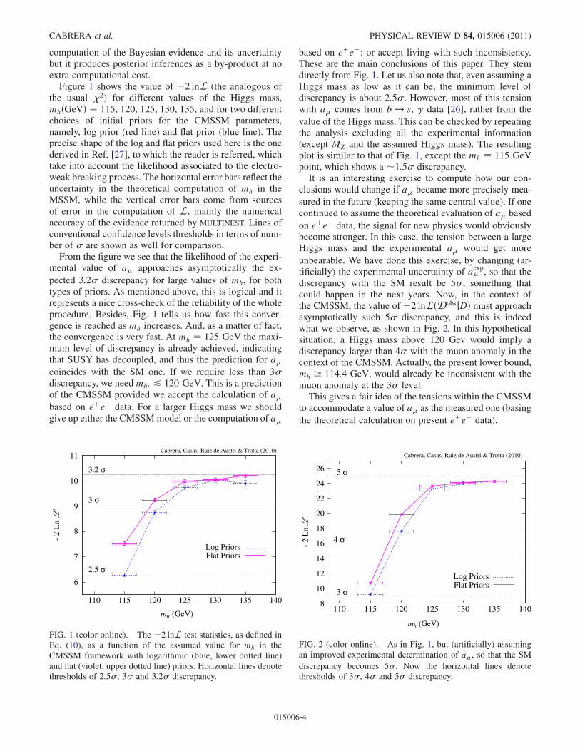
Figure 1 shows the value of �2 lnL (the analogous ofthe usual 2) for different values of the Higgs mass,mhðGeVÞ ¼ 115, 120, 125, 130, 135, and for two differentchoices of initial priors for the CMSSM parameters,namely, log prior (red line) and flat prior (blue line). Theprecise shape of the log and flat priors used here is the onederived in Ref. [27], to which the reader is referred, whichtake into account the likelihood associated to the electro-weak breaking process. The horizontal error bars reflect theuncertainty in the theoretical computation of mh in theMSSM, while the vertical error bars come from sourcesof error in the computation of L, mainly the numericalaccuracy of the evidence returned by MULTINEST. Lines ofconventional confidence levels thresholds in terms of num-ber of � are shown as well for comparison.

From the figure we see that the likelihood of the experi-mental value of a� approaches asymptotically the ex-

pected 3:2� discrepancy for large values of mh, for bothtypes of priors. As mentioned above, this is logical and itrepresents a nice cross-check of the reliability of the wholeprocedure. Besides, Fig. 1 tells us how fast this conver-gence is reached as mh increases. And, as a matter of fact,the convergence is very fast. At mh ¼ 125 GeV the maxi-mum level of discrepancy is already achieved, indicatingthat SUSY has decoupled, and thus the prediction for a�coincides with the SM one. If we require less than 3�discrepancy, we needmh: & 120 GeV. This is a predictionof the CMSSM provided we accept the calculation of a�based on eþe� data. For a larger Higgs mass we shouldgive up either the CMSSMmodel or the computation of a�

based on eþe�; or accept living with such inconsistency.These are the main conclusions of this paper. They stemdirectly from Fig. 1. Let us also note that, even assuming aHiggs mass as low as it can be, the minimum level ofdiscrepancy is about 2:5�. However, most of this tensionwith a� comes from b ! s, data [26], rather from the

value of the Higgs mass. This can be checked by repeatingthe analysis excluding all the experimental information(except MZ and the assumed Higgs mass). The resultingplot is similar to that of Fig. 1, except the mh ¼ 115 GeVpoint, which shows a �1:5� discrepancy.It is an interesting exercise to compute how our con-

clusions would change if a� became more precisely mea-

sured in the future (keeping the same central value). If onecontinued to assume the theoretical evaluation of a� based

on eþe� data, the signal for new physics would obviouslybecome stronger. In this case, the tension between a largeHiggs mass and the experimental a� would get more

unbearable. We have done this exercise, by changing (ar-tificially) the experimental uncertainty of aexp� , so that thediscrepancy with the SM result be 5�, something thatcould happen in the next years. Now, in the context ofthe CMSSM, the value of �2 lnLðDobsjDÞ must approachasymptotically such 5� discrepancy, and this is indeedwhat we observe, as shown in Fig. 2. In this hypotheticalsituation, a Higgs mass above 120 Gev would imply adiscrepancy larger than 4� with the muon anomaly in thecontext of the CMSSM. Actually, the present lower bound,mh � 114:4 GeV, would already be inconsistent with themuon anomaly at the 3� level.This gives a fair idea of the tensions within the CMSSM

to accommodate a value of a� as the measured one (basing

the theoretical calculation on present eþe� data).

6

7

8

9

10

11

110 115 120 125 130 135 140

-2

Ln

mh (GeV)

2.5 σ

3 σ

3.2 σ

Cabrera, Casas, Ruiz de Austri & Trotta (2010)

Log PriorsFlat Priors

FIG. 1 (color online). The �2 lnL test statistics, as defined inEq. (10), as a function of the assumed value for mh in theCMSSM framework with logarithmic (blue, lower dotted line)and flat (violet, upper dotted line) priors. Horizontal lines denotethresholds of 2:5�, 3� and 3:2� discrepancy.

8

10

12

14

16

18

20

22

24

26

110 115 120 125 130 135 140

-2

Ln

mh (GeV)

3 σ

4 σ

5 σ

Cabrera, Casas, Ruiz de Austri & Trotta (2010)

Log PriorsFlat Priors

FIG. 2 (color online). As in Fig. 1, but (artificially) assumingan improved experimental determination of a�, so that the SM

discrepancy becomes 5�. Now the horizontal lines denotethresholds of 3�, 4� and 5� discrepancy.

CABRERA et al. PHYSICAL REVIEW D 84, 015006 (2011)

015006-4

IV. PROBABILITY DISTRIBUTIONS FORSUPERSYMMETRIC PARAMETERS

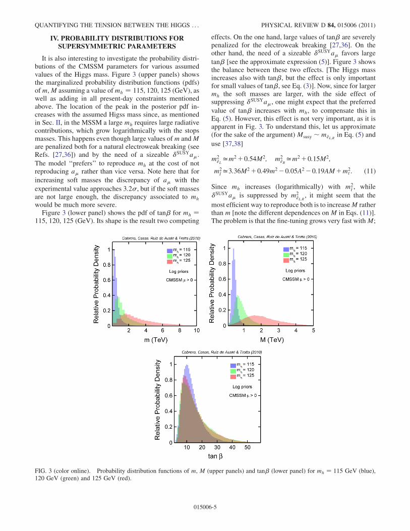
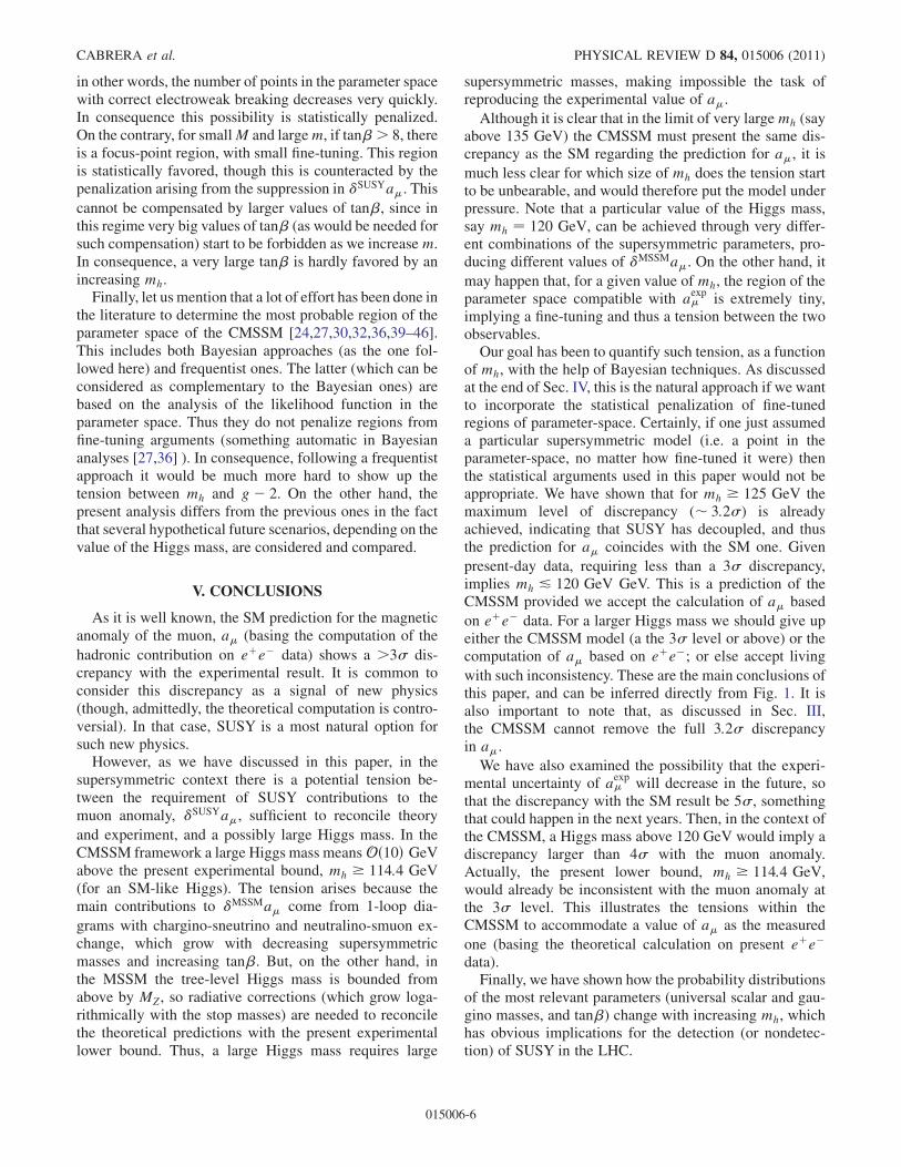
It is also interesting to investigate the probability distri-butions of the CMSSM parameters for various assumedvalues of the Higgs mass. Figure 3 (upper panels) showsthe marginalized probability distribution functions (pdfs)ofm,M assuming a value ofmh ¼ 115, 120, 125 (GeV), aswell as adding in all present-day constraints mentionedabove. The location of the peak in the posterior pdf in-creases with the assumed Higss mass since, as mentionedin Sec. II, in the MSSM a large mh requires large radiativecontributions, which grow logarithmically with the stopsmasses. This happens even though large values ofm andMare penalized both for a natural electroweak breaking (seeRefs. [27,36]) and by the need of a sizeable �SUSYa�.

The model ‘‘prefers’’ to reproduce mh at the cost of notreproducing a� rather than vice versa. Note here that for

increasing soft masses the discrepancy of a� with the

experimental value approaches 3:2�, but if the soft massesare not large enough, the discrepancy associated to mh

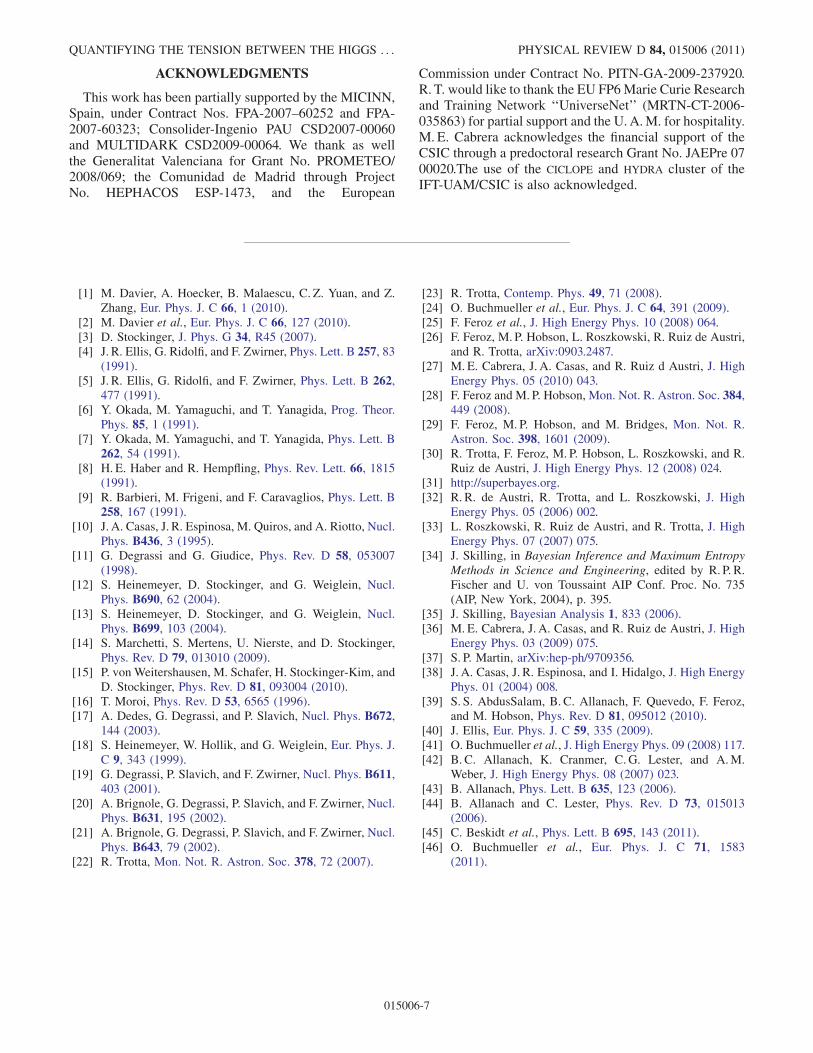
would be much more severe.Figure 3 (lower panel) shows the pdf of tan� for mh ¼

115, 120, 125 (GeV). Its shape is the result two competing

effects. On the one hand, large values of tan� are severelypenalized for the electroweak breaking [27,36]. On theother hand, the need of a sizeable �SUSYa� favors large

tan� [see the approximate expression (5)]. Figure 3 showsthe balance between these two effects. [The Higgs massincreases also with tan�, but the effect is only importantfor small values of tan�, see Eq. (3)]. Now, since for largermh the soft masses are larger, with the side effect ofsuppressing �SUSYa�, one might expect that the preferred

value of tan� increases with mh, to compensate this inEq. (5). However, this effect is not very important, as it isapparent in Fig. 3. To understand this, let us approximate(for the sake of the argument) Msusy �m~eL;R in Eq. (5) and

use [37,38]

m2~eL’m2þ0:54M2; m2

~eR’m2þ0:15M2;

m2~t ’3:36M2þ0:49m2�0:05A2�0:19AMþm2

t : (11)

Since mh increases (logarithmically) with m2~t , while

�SUSYa� is suppressed by m2~eL;R

, it might seem that the

most efficient way to reproduce both is to increaseM ratherthan m [note the different dependences onM in Eqs. (11)].The problem is that the fine-tuning grows very fast withM;

FIG. 3 (color online). Probability distribution functions of m, M (upper panels) and tan� (lower panel) for mh ¼ 115 GeV (blue),120 GeV (green) and 125 GeV (red).

QUANTIFYING THE TENSION BETWEEN THE HIGGS . . . PHYSICAL REVIEW D 84, 015006 (2011)

015006-5

in other words, the number of points in the parameter spacewith correct electroweak breaking decreases very quickly.In consequence this possibility is statistically penalized.On the contrary, for smallM and largem, if tan�> 8, thereis a focus-point region, with small fine-tuning. This regionis statistically favored, though this is counteracted by thepenalization arising from the suppression in �SUSYa�. This

cannot be compensated by larger values of tan�, since inthis regime very big values of tan� (as would be needed forsuch compensation) start to be forbidden as we increasem.In consequence, a very large tan� is hardly favored by anincreasing mh.

Finally, let us mention that a lot of effort has been done inthe literature to determine the most probable region of theparameter space of the CMSSM [24,27,30,32,36,39–46].This includes both Bayesian approaches (as the one fol-lowed here) and frequentist ones. The latter (which can beconsidered as complementary to the Bayesian ones) arebased on the analysis of the likelihood function in theparameter space. Thus they do not penalize regions fromfine-tuning arguments (something automatic in Bayesiananalyses [27,36] ). In consequence, following a frequentistapproach it would be much more hard to show up thetension between mh and g� 2. On the other hand, thepresent analysis differs from the previous ones in the factthat several hypothetical future scenarios, depending on thevalue of the Higgs mass, are considered and compared.

V. CONCLUSIONS

As it is well known, the SM prediction for the magneticanomaly of the muon, a� (basing the computation of the

hadronic contribution on eþe� data) shows a >3� dis-crepancy with the experimental result. It is common toconsider this discrepancy as a signal of new physics(though, admittedly, the theoretical computation is contro-versial). In that case, SUSY is a most natural option forsuch new physics.

However, as we have discussed in this paper, in thesupersymmetric context there is a potential tension be-tween the requirement of SUSY contributions to themuon anomaly, �SUSYa�, sufficient to reconcile theory

and experiment, and a possibly large Higgs mass. In theCMSSM framework a large Higgs mass meansOð10Þ GeVabove the present experimental bound, mh � 114:4 GeV(for an SM-like Higgs). The tension arises because themain contributions to �MSSMa� come from 1-loop dia-

grams with chargino-sneutrino and neutralino-smuon ex-change, which grow with decreasing supersymmetricmasses and increasing tan�. But, on the other hand, inthe MSSM the tree-level Higgs mass is bounded fromabove by MZ, so radiative corrections (which grow loga-rithmically with the stop masses) are needed to reconcilethe theoretical predictions with the present experimentallower bound. Thus, a large Higgs mass requires large

supersymmetric masses, making impossible the task ofreproducing the experimental value of a�.

Although it is clear that in the limit of very largemh (sayabove 135 GeV) the CMSSM must present the same dis-crepancy as the SM regarding the prediction for a�, it is

much less clear for which size of mh does the tension startto be unbearable, and would therefore put the model underpressure. Note that a particular value of the Higgs mass,say mh ¼ 120 GeV, can be achieved through very differ-ent combinations of the supersymmetric parameters, pro-ducing different values of �MSSMa�. On the other hand, it

may happen that, for a given value of mh, the region of theparameter space compatible with aexp� is extremely tiny,implying a fine-tuning and thus a tension between the twoobservables.Our goal has been to quantify such tension, as a function

of mh, with the help of Bayesian techniques. As discussedat the end of Sec. IV, this is the natural approach if we wantto incorporate the statistical penalization of fine-tunedregions of parameter-space. Certainly, if one just assumeda particular supersymmetric model (i.e. a point in theparameter-space, no matter how fine-tuned it were) thenthe statistical arguments used in this paper would not beappropriate. We have shown that for mh � 125 GeV themaximum level of discrepancy (� 3:2�) is alreadyachieved, indicating that SUSY has decoupled, and thusthe prediction for a� coincides with the SM one. Given

present-day data, requiring less than a 3� discrepancy,implies mh & 120 GeV GeV. This is a prediction of theCMSSM provided we accept the calculation of a� based

on eþe� data. For a larger Higgs mass we should give upeither the CMSSM model (a the 3� level or above) or thecomputation of a� based on eþe�; or else accept living

with such inconsistency. These are the main conclusions ofthis paper, and can be inferred directly from Fig. 1. It isalso important to note that, as discussed in Sec. III,the CMSSM cannot remove the full 3:2� discrepancyin a�.

We have also examined the possibility that the experi-mental uncertainty of a

exp� will decrease in the future, so

that the discrepancy with the SM result be 5�, somethingthat could happen in the next years. Then, in the context ofthe CMSSM, a Higgs mass above 120 GeV would imply adiscrepancy larger than 4� with the muon anomaly.Actually, the present lower bound, mh � 114:4 GeV,would already be inconsistent with the muon anomaly atthe 3� level. This illustrates the tensions within theCMSSM to accommodate a value of a� as the measured

one (basing the theoretical calculation on present eþe�data).Finally, we have shown how the probability distributions

of the most relevant parameters (universal scalar and gau-gino masses, and tan�) change with increasing mh, whichhas obvious implications for the detection (or nondetec-tion) of SUSY in the LHC.

CABRERA et al. PHYSICAL REVIEW D 84, 015006 (2011)

015006-6

ACKNOWLEDGMENTS

This work has been partially supported by the MICINN,Spain, under Contract Nos. FPA-2007–60252 and FPA-2007-60323; Consolider-Ingenio PAU CSD2007-00060and MULTIDARK CSD2009-00064. We thank as wellthe Generalitat Valenciana for Grant No. PROMETEO/2008/069; the Comunidad de Madrid through ProjectNo. HEPHACOS ESP-1473, and the European

Commission under Contract No. PITN-GA-2009-237920.R. T. would like to thank the EU FP6Marie Curie Researchand Training Network ‘‘UniverseNet’’ (MRTN-CT-2006-035863) for partial support and the U.A.M. for hospitality.M. E. Cabrera acknowledges the financial support of theCSIC through a predoctoral research Grant No. JAEPre 0700020.The use of the CICLOPE and HYDRA cluster of theIFT-UAM/CSIC is also acknowledged.

[1] M. Davier, A. Hoecker, B. Malaescu, C. Z. Yuan, and Z.Zhang, Eur. Phys. J. C 66, 1 (2010).

[2] M. Davier et al., Eur. Phys. J. C 66, 127 (2010).[3] D. Stockinger, J. Phys. G 34, R45 (2007).[4] J. R. Ellis, G. Ridolfi, and F. Zwirner, Phys. Lett. B 257, 83

(1991).[5] J. R. Ellis, G. Ridolfi, and F. Zwirner, Phys. Lett. B 262,

477 (1991).[6] Y. Okada, M. Yamaguchi, and T. Yanagida, Prog. Theor.

Phys. 85, 1 (1991).[7] Y. Okada, M. Yamaguchi, and T. Yanagida, Phys. Lett. B

262, 54 (1991).[8] H. E. Haber and R. Hempfling, Phys. Rev. Lett. 66, 1815

(1991).[9] R. Barbieri, M. Frigeni, and F. Caravaglios, Phys. Lett. B

258, 167 (1991).[10] J. A. Casas, J. R. Espinosa, M. Quiros, and A. Riotto, Nucl.

Phys. B436, 3 (1995).[11] G. Degrassi and G. Giudice, Phys. Rev. D 58, 053007

(1998).[12] S. Heinemeyer, D. Stockinger, and G. Weiglein, Nucl.

Phys. B690, 62 (2004).[13] S. Heinemeyer, D. Stockinger, and G. Weiglein, Nucl.

Phys. B699, 103 (2004).[14] S. Marchetti, S. Mertens, U. Nierste, and D. Stockinger,

Phys. Rev. D 79, 013010 (2009).[15] P. vonWeitershausen, M. Schafer, H. Stockinger-Kim, and

D. Stockinger, Phys. Rev. D 81, 093004 (2010).[16] T. Moroi, Phys. Rev. D 53, 6565 (1996).[17] A. Dedes, G. Degrassi, and P. Slavich, Nucl. Phys. B672,

144 (2003).[18] S. Heinemeyer, W. Hollik, and G. Weiglein, Eur. Phys. J.

C 9, 343 (1999).[19] G. Degrassi, P. Slavich, and F. Zwirner, Nucl. Phys. B611,

403 (2001).[20] A. Brignole, G. Degrassi, P. Slavich, and F. Zwirner, Nucl.

Phys. B631, 195 (2002).[21] A. Brignole, G. Degrassi, P. Slavich, and F. Zwirner, Nucl.

Phys. B643, 79 (2002).[22] R. Trotta, Mon. Not. R. Astron. Soc. 378, 72 (2007).

[23] R. Trotta, Contemp. Phys. 49, 71 (2008).[24] O. Buchmueller et al., Eur. Phys. J. C 64, 391 (2009).[25] F. Feroz et al., J. High Energy Phys. 10 (2008) 064.[26] F. Feroz, M. P. Hobson, L. Roszkowski, R. Ruiz de Austri,

and R. Trotta, arXiv:0903.2487.[27] M. E. Cabrera, J. A. Casas, and R. Ruiz d Austri, J. High

Energy Phys. 05 (2010) 043.[28] F. Feroz and M. P. Hobson, Mon. Not. R. Astron. Soc. 384,

449 (2008).[29] F. Feroz, M. P. Hobson, and M. Bridges, Mon. Not. R.

Astron. Soc. 398, 1601 (2009).[30] R. Trotta, F. Feroz, M. P. Hobson, L. Roszkowski, and R.

Ruiz de Austri, J. High Energy Phys. 12 (2008) 024.[31] http://superbayes.org.[32] R. R. de Austri, R. Trotta, and L. Roszkowski, J. High

Energy Phys. 05 (2006) 002.[33] L. Roszkowski, R. Ruiz de Austri, and R. Trotta, J. High

Energy Phys. 07 (2007) 075.[34] J. Skilling, in Bayesian Inference and Maximum Entropy

Methods in Science and Engineering, edited by R. P. R.Fischer and U. von Toussaint AIP Conf. Proc. No. 735(AIP, New York, 2004), p. 395.

[35] J. Skilling, Bayesian Analysis 1, 833 (2006).[36] M. E. Cabrera, J. A. Casas, and R. Ruiz de Austri, J. High

Energy Phys. 03 (2009) 075.[37] S. P. Martin, arXiv:hep-ph/9709356.[38] J. A. Casas, J. R. Espinosa, and I. Hidalgo, J. High Energy

Phys. 01 (2004) 008.[39] S. S. AbdusSalam, B. C. Allanach, F. Quevedo, F. Feroz,

and M. Hobson, Phys. Rev. D 81, 095012 (2010).[40] J. Ellis, Eur. Phys. J. C 59, 335 (2009).[41] O. Buchmueller et al., J. High Energy Phys. 09 (2008) 117.[42] B. C. Allanach, K. Cranmer, C. G. Lester, and A.M.

Weber, J. High Energy Phys. 08 (2007) 023.[43] B. Allanach, Phys. Lett. B 635, 123 (2006).[44] B. Allanach and C. Lester, Phys. Rev. D 73, 015013

(2006).[45] C. Beskidt et al., Phys. Lett. B 695, 143 (2011).[46] O. Buchmueller et al., Eur. Phys. J. C 71, 1583

(2011).

QUANTIFYING THE TENSION BETWEEN THE HIGGS . . . PHYSICAL REVIEW D 84, 015006 (2011)

015006-7