In the Name of Allah,

the Beneficent, the Merciful

Model Predictive Impedance Control: A Model for Joint Movement Control

A thesis Submitted to the College of Graduate Studies and Research

in Partial Fulfillment of the Requirements For the Degree of

DOCTOR OF PHILOSOPHY

in the Division of Biomedical Engineering

University of Saskatchewan

by

Farzad Towhidkhah

Saskatoon, Saskatchewan, Canada

August 1996

© The author claims copyright. Use shall not be made of the material contained herein without proper acknowledgment as indicated on the copyright page.

ii

COPYRIGHT

The author has agreed that the library, University of Saskatchewan, may make this thesis freely available for inspections. Moreover, the author has agreed that permission for extensive copying of this thesis of scholarly purpose may be granted by the professor or professors who supervised the thesis work recorded herein or, in their absence, by the head of the Department or the Dean of the College in which the thesis work was done. It is understood that due recognition will be given to the author of this thesis and to the University of Saskatchewan in any use of the material in this thesis. Copying or publication or any other use of the thesis for financial gain without approval by the University of Saskatchewan and the author’s written permission is prohibited. Request for permission to copy or to make other use of material in this thesis in whole or in part should be addressed to :

Chair of the Division of Biomedical Engineering, University of Saskatchewan, 57 Campus Dr., Saskatoon, Saskatchewan, Canada, S7N 5A9.

iii

University of Saskatchewan

Division of Biomedical Engineering

Model Predictive Impedance Control: A Model for Joint Movement Control

Student: Farzad Towhidkhah Supervisors: Dr. R. E. Gander Dr. H. C. Wood

Ph.D. Thesis Submitted to the College of Graduate Studies and Research

August 1996

ABSTRACT

A human is capable of making various movements under different environmental

conditions including highly accurate movements, low accurate movements, ballistic

movements, or learning new skills. This flexibility results from highly integrated neural

centers in the brain and the spinal cord acting as higher and lower level controllers and

information processors, a large number of muscles and bones constructing the actuators

required to generate movements, and numerous sensory receptors informing the neural

centers about the results of movement and the environment. For a comprehensive

understanding of the motor control system, it is necessary to have a global model. This

iv

model can also be used to test the function of motor components under natural or

pathological conditions.

This thesis is an effort toward developing such a global model based on the most

currently accepted theories and hypotheses in biological motor control and control

engineering. The proposed model, called model predictive impedance control,

specifically combines the equilibrium point hypothesis (α and λ models), the impedance

control strategy (including stiffness and viscosity), servomechanism control theory, and

the optimization-based model predictive control algorithm as a unified model applicable

in the study of different types of movements. The model is adaptive with learning ability

and operates in open-loop or closed-loop manners. The focus is on the overall function of

motor centers instead of individual realization structurally or functionally. Acting as a

supervisory and higher level controller, the model predictive controller presents a new

approach to determine the joint impedance and the equilibrium point based on use of a

priori knowledge of the neuromusculoskeletal system and environment.

To evaluate the performance of the model, it was applied to three different types

of joint movements: a tracking movement with an unpredicted disturbance, a rhythmic

movement, and an unstable biped model of human walking. Computer simulation results

showed excellent performance of the model in all three cases for optimal values of active

joint impedances and a perfect match between the musculoskeletal system and the model

internal to the model predictive controller. The controller was also able to maintain

acceptable performance in the presence of a 25% mismatch between the musculoskeletal

system and its internal model.

v

ACKNOWLEDGMENTS

All praise is due to Allah who guided us to this, and we would not have found the way had it not been that Allah guided us.( Holy Qur’an, Ch. 7, Ver. 43)

Thanks God, the first and last biomedical engineer, for creation of this fascinating nature. Thanks God for creation of human who He willed to be His deputy on the earth. Thanks God for giving human thinking and learning abilities to study the beauties of the nature and learn from it. Thanks God for giving me a chance to have a little contribution on the study of the wonderful field of human motor system which compared to it, man-made systems are only simple toys. Whoever is ungrateful to the people, he is ungrateful to the creator, (Prophet Mohammad). I sincerely wish to thank my supervisors, Professors R. E. Gander and H. C. Wood, not only for their valuable advice, encouragement, and guidance, but also for their personal friendship that has made my graduate program so productive. Without their help and patience, this dissertation would have been impossible. Special thanks go to Drs. B. R. Brandell and G. R. Colborne at the Department of Anatomy for their feedback and comments on biological aspects of preliminary versions of the thesis. I am also very grateful to Professors P. N. Nikiforuk and C. M. Sargent for their effort and time in reading the dissertation and serving on the advisory committee. Many thanks go to my colleague Dr. M. Ashobi for his invaluable discussion on control systems as well as his particular help on the neural network simulation. It is a pleasure to show my gratitude to K. Tischler, International Student Advisor, for his help and support, and to Jonathan Moor, Ian McPhedran, and Keith Jeffrey for their technical assistance in computer services. I would like to express my sincere appreciation to my wife, Mojdeh Radjabi, for her patience, encouragement, and moral support. Financial support provided by the Ministry of Culture and Higher Education of Islamic Republic of Iran, the University of Saskatchewan, and NSERC operating grant are gratefully acknowledged.

vi

This dissertation is dedicated

to

my parents

and to

my wife

vii

TABLE OF CONTENTS Contents Page Copyright ......................................................................................... iii Abstract ........................................................................................... iv Acknowledgments ............................................................................ vi Dedication ....................................................................................... vii Table of Contents ............................................................................. viii List of Figures .................................................................................. x List of Tables .................................................................................... xv List of Abbreviations and Symbols ..................................................... xvi Chapter 1- Biological Motor System Modeling .............................. 1 1.1 Biological Motor Control ................................................. 2 1.1.1. Motor Control Centers ...................................... 2 - The Motor Cortex ......................................... 4 - The Cerebellum ............................................. 5 -The Spinal Cord ............................................. 5 1.1.2 Sensory Feedback ............................................... 7 1.1.3 Motor Control Modes ......................................... 7 - Closed-Loop and Open-Loop Modes ............. 8 - Motor Program .............................................. 9 - Equilibrium Point Hypothesis ......................... 10 - Hierarchical Structure .................................... 10 1.2 Scope of This Thesis ......................................................... 11 1.3 Objectives of the Thesis ..................................................... 13 Chapter 2- Basis for Model Predictive Impedance Control ............ 16 2.1 Impedance Control Strategy ............................................... 16 2.1.1 Stiffness Control Strategy and Equilibrium Point Hypothesis ............................ 17 2.1.2 Impedance Control Strategy and Generalization of EPH ...................................... 22 2.2 Optimization-Based Strategies ............................................ 25 2.3 Model-Based Strategies ...................................................... 27 2.4 Model Predictive Control Algorithm ................................... 30 2.5 Summary ............................................................................ 33

viii

Chapter 3- Identification of the Neuromusculoskeletal System Using Neural Networks ................................................... 36

3.1 Neural Network Background .............................................. 37 3.2 Neural Network Modeling .................................................. 41 3.3 Modeling the Neuromusculoskeletal System ........................ 43 3.4 Computer Simulation and Results ....................................... 47 3.5 Discussion .......................................................................... 52

Chapter 4- Model Predictive Impedance Control Scheme ............... 54 4.1 A Scheme for Joint Movement Control Using Stiffness Regulation ............................................. 54 4.1.1 Computer Simulation and Results ......................... 57 4.1.2 Discussion ............................................................ 60 4.2 A Comparison Between MPC and the Smith Predictor ........ 63 4.3 Model Predictive Impedance Control Scheme ...................... 71 4.4 Discussion ........................................................................... 77 4.5 Summary ............................................................................. 80 Chapter 5- Application of the Model Predictive Impedance Control Scheme ......................................................................... 81 5.1 Rhythmic Movement ........................................................... 82 5.2 Tracking Movement ............................................................ 86 5.3 Biped Model for Walking .................................................... 89 5.4 System and Model Mismatch ............................................... 93 5.4.1 System Parameters Mismatch ................................ 93 5.4.2 External Disturbance Mismatch ............................. 95 5.4.3- Applying Neural Network Model ......................... 96 5.5 Effects of Changing the Horizon Factors ............................. 97 5.6 Discussion ........................................................................... 102 Chapter 6- Summary and Future Directions ..................................... 106 6.1 Summary ............................................................................. 106 6.2 Fulfilling the Objectives ....................................................... 111 6.3 Future Directions ................................................................. 113 6.4 Conclusion ........................................................................... 114 References ............................................................................................ 115 Appendix: Calculation of the Sensitivity Function ............................ 124

ix

LIST OF FIGURES

Figure Page Chapter 1

Fig. 1-1 A simplified biological structure of the human motor system. .. 3 Fig. 1-2 A simplified block diagram of hierarchical control system. .... 12

Chapter 2

Fig. 2-1 Principle of the stiffness control strategy. ............................ 20 Fig. 2-2 The basis of equilibrium point hypothesis.σ is the

incremental joint stiffness and β is the slack angle. .................... 20

Fig. 2-3 A new equilibrium position as a shift in net characteristic. Point 1 is the initial position and point 2 is the final position. ...... 21

Fig 2-4 The effect of disturbance on change of equilibrium position.βv is the virtual equilibrium point. σ is the joint stiffness.θi is initial and θf is the desired positions. Td represents the external disturbance. .............................................................................. 21

Fig 2-5 3-D active muscles characteristic. ........................................ 23 Fig. 2-6 Principle of the 3-D equilibrium point hypothesis. The

three dimensional surface is the new net characteristic of antagonist muscles. P represents the current output state, and Q represents the desired output state or equilibrium point. The solid line represents the load-disturbance characteristic which intersects the net muscle characteristic at point Q. The vector for P to Q represents the error which generates the torque required to establish the new equilibrium point. β is the slack angle, and β

. is

the slack angular velocity. .......................................................... 24

x

Fig. 2-7 The principle of model predictive control. The three dimensional surface is the new net characteristic of antagonist muscles. P represents the current output state, and Q represents the desired output state or equilibrium point. The solid line represents the load-disturbance characteristic which intersects the net muscle characteristic at point Q. The vector for P to Q represents the error which generates the torque required to establish the new equilibrium point. β is the slack angle, and β

.

is the slack angular velocity. ........................................................... 32

Chapter 3

Fig. 3-1 a) A biological neuron. b) An engineering neuron. ............... 38 Fig. 3-2 Learning methods: a) supervised method,

b) unsupervised method. ............................................................. 39

Fig. 3-3 Tapped delay lines dynamic neural network. ........................ 42 Fig. 3-4 Fully recurrent Hopfield neural network model (network a). ... 44 Fig 3-5 Modified Hopfield neural networks. b is state the feedback

network, c is the state-output feedback network, d is the output feedback network, e is the Jordan network. ................................ 45

Fig. 3-6 Training errors for different neural networks ( models a-e). .. 49 Fig. 3-7 Training errors for the state feedback network for different

starting points. ........................................................................... 49 Fig. 3-8a Dynamic responses (test results) for different neural

networks. ................................................................................... 50 Fig. 3-8b Dynamic response (test result) for the state feedback

network (model b). .................................................................... 51

Chapter 4

Fig. 4-1 The schematic diagram for adjusting the joint stiffnessand slack angle. θd is desired joint angle trajectory; θ, actual joint angle trajectory; σ, active joint stiffness; β, slack angle trajectory and Td, the external disturbance. ................................................ 55

xi

Fig. 4-2 The mathematical model of the stiffness control strategy. G(s) is the dynamics of joint-load; Gf(s), the transfer function of the feedforward pathway for external disturbance; and βv, the virtual equilibrium point. ............................................................ 55

Fig. 4-3 a) The slack angle (β), b) the desired position (θd) and

actual position (θ) for case 1 (σ=67 Nm/rad and Td=0). ............. 58 Fig. 4-4 The effect of disturbance in case 2 (no receptor dynamics

and no delay pathways). a) Td=10 Nm. b) Td=30 Nm. ................ 59 Fig. 4-5 The effect of change of disturbance and stiffness on the

error. The solid curve is θd, the dashed curve is θ and the dash-point curve is the error. σ=10, 25, 40, 55, 70 Nm/rad. The arrows show the direction of increasing of σ. a) Td=0 Nm. b) Td=-15 Nm. c) Td=15 Nm. d) Td=30 Nm. e) Td=-30 Nm. ....... 60

Fig. 4-6 Two systems with time delay. a) delay in feedback,

b) delay in feedforward. ............................................................. 62 Fig. 4-7 The Smith predictor control scheme. Gm(s) is the plant

model, G*(s) is plant model with no time delay, θd is desired output, θ is actual output, and β is the control signal. ................ 63

Fig. 4-8 The model predictive control scheme. θd is desired output,

θ is actual output, θm is the model output, Td is the external disturbance, and β is the control signal. ..................................... 64

Fig. 4-9 Comparison between the Smith predictor and model predictive control outputs for a) perfect models, ..................................................................... 66 b) time delay mismatch, ............................................................ 67 c) filter mismatch, ..................................................................... 68 d) time delay and filter mismatch, .............................................. 69 e) non-minimum phase system. .................................................. 70 Fig. 4-10 The model predictive impedance control scheme. θd and

θ.

d are desired joint angle and angular velocity. θ and θ.

are actual joint angle and angular velocity. θm is measured joint angle. Td is the external disturbance. G1(s) and G2(s) are dynamics relating to the generation of EMG signal and muscles’ torque; and G3(s) is joint-load dynamics. .................................... 73

xii

Chapter 5

Fig. 5-1 Error function with respect to joint stiffness (Nm/rad) and viscosity (Nms/rad) for the rhythmic movement. ........................ 84

Fig. 5-2 Desired joint angle trajectory (solid curve) and model’s

output trajectory (dotted curve) for optimal values of joint impedance for the rhythmic movement. I shows the swing phase and II shows the standing phase. a) for M=3 and P=20. b) for M=20 and P=50. ........................................................................ 85

Fig. 5-3 Error function with respect to joint stiffness (Nm/rad) and

viscosity (Nms/rad) for the tracking movement. .......................... 87 Fig. 5-4 A comparison of the desired trajectory (solid curve) and

output trajectory (dotted curve). a) for nonoptimal values of joint impedance, σ = 70 Nm/rad, and b = 0. Total root square error is 1.18 rad. b) for optimal values of joint impedance, σ = 60 Nm/rad, and b = 35 Nms/rad. Total root square error is 0.2 rad. ...................................................................................... 88

Fig. 5-5 The biped model for human walking. γ is the angle of the

swinging leg, θ is the angle of standing leg, m is the mass of body and m1 is the mass of the swinging leg. HAT represents head, arms, and trunk. ................................................................ 90

Fig. 5-6 The simulation procedure for the study of biped model. X0

is the initial condition. The switch condition 1 is for identification of the system and the switch condition 2 is for control of the system. ....................................................................................... 91

Fig. 5-7 a) Desired joint angle trajectory (solid curve) and model’s

output trajectory (dotted curve) for optimal values of joint impedance for walking study. b) Variations of the system impulse response in walking cycle intervals. ................................ 92

Fig. 5-8 (a) Different disturbances applied to the model. Dist (solid

curve) is the disturbance model used, Dist-p (dashed curve) is the disturbance applied to the system with positive mismatch, and Dist-n (dotted curve) is the disturbance applied to the system with negative mismatch. (b) The results of disturbance mismatch test. Output (solid curve), Output-p (dashed curve), and Output-n (dotted curve) are outputs regarding to the application of Dist, Dist-p, and Dist-n to the system respectively. ............................................................................... 95

xiii

Fig. 5-9 Step responses of the neuromusculoskeletal system and its

neural network model. ................................................................ 96 Fig. 5-10 The results of application of neural network model in

control of the neuromusculoskeletal system for the tracking movement. ................................................................................. 97

Fig. 5-11 The results of changes in minimum errors due to changes

in horizons and degree of mismatch for the rhythmic movement. For horizontal axis: 1 means M=3 and P=10, 2, M=3 and P=20, 3, M=3 and P=30, 4, M=3 and P=40, 5, M=3 and P=50, 6, M=10 and P=25, 7, M=10 and P=50, and 8, M=25 and P=50. ... 99

Fig. 5-12 The variations of the optimal points with respect to

horizons and degree of mismatch for the rhythmic movement. .... 100 Fig. 5-13 The results of changes in minimum errors due to changes

in horizons and degree of mismatch for the tracking movement. For horizontal axis: 1 means M=3 and P=10, 2, M=3 and P=20, 3, M=3 and P=30, 4, M=3 and P=40, 5, M=3 and P=50, 6, M=10 and P=25, 7, M=10 and P=50, and 8, M=25 and P=50. ... 101

Fig. 5-14 The variations of the optimal points with respect to

horizons and degree of mismatch for the tracking movement. ...... 102

xiv

LIST OF TABLES Table Page Chapter 3

Table 3-1 A summary of relative training error, test error, and computational time for different models. ........................... 52

Chapter 4

Table 4-1 A summary of the plant and the models applied in test of the Smith predictor and the model predictive control. .......... 65 Table 4-2 A summary of the errors for Smith Predictor and model predictive controllers. ................................................... 65

Chapter 5

Table 5-1 The root square errors for parameter mismatch in the rhythmic movement study. ............................................ 93 Table 5-2 The root square errors for parameter mismatch in the tracking movement study. ............................................. 94 Table 5-3 The optimal root square errors for parameter mismatch in the tracking movement study. ............................................ 94

xv

LIST OF ABBREVIATIONS AND SYMBOLS Abbreviations MPIC: Model Predictive Impedance Control MPC: Model Predictive Control SP: Smith Predictor SPC: Smith Predictor Controller EMG: Electromyogram EP: Equilibrium Point EPH: Equilibrium Point Hypothesis CNS: Central Nervous System GA: Genetic Algorithm ARMA: Auto-Regressive Moving Average PD: Proportional and Derivitive CPG: Central Pattern Generators FNS: Functional Neuromuscular Stimulation Symbols b1: active joint viscosity, Nms/rad B: joint passive viscosity, Nms/rad d: unmeasurable disturbance, Nm Dist: Disturbance Dist-p: Positive Disturbance Dist-n: Negative Disturbance dh(k): teaching signal for output h f: neuron nonlinear output function G*: plant model with no time delay g: gravitational acceleration, m/s2

G1: dynamics relating to the generation of the myoelectric signal G2: dynamics relating to the generation of muscle forces G3: joint-load dynamics Gc: controller gain Gf: feedfoward gain Gm: plant model I: joint inertia, kgm2

J: cost function 1 In this thesis, bold style is used to distinguish the variables from the simple characters.

xvi

K: passive joint stiffness l: length of standing leg, m l1: distance between the hip joint and the swinging leg mass center, m M: control (input) horizon m: weight of the body and trunk, Kg m1: weight of the swinging leg, kg Nin: number of neural network inputs Nou: number of the outputs Npat: length of the data set P: model (prediction) horizon qk: error weighting factor rk: control signal weighting factor sh(k): sensitivity of the output with respect to w T: muscles’ torque T1: time constant of generating the neural drive, ms T2: time constant of generating the muscles’ torque, ms Td: External Disturbance, N td: time delay, ms uh: the hth neuron input. w: synaptic weight, wc: plant bandwidth, rad/s wh: the hth synaptic weight wm: model bandwidth, rad/s X0: initial conditions y: neuron output Greek Symbols β: slack angle (equilibrium angle), rad

v: vertual slack angle, rad β

θ

θ

β.

: slack angular velocity (equilibrium angular velocity), rad/s γ: angle of the swinging leg, degree σ: active joint stiffness, Nm/rad

: actual joint angle θ.

: actual joint angular velocity, rad/s θf: final joint angle, rad

d: desired joint angle, rad

θ.

d: desired joint angular velocity, rad/s θp: predicted joint angle, rad θm: model output, rad µ: learning gain (factor)

xvii

CHAPTER 1- BIOLOGICAL MOTOR SYSTEM MODELING

Although human movement appears to be a relatively simple attribute, it is a very

complex and challenging phenomenon to understand. Over the last century, many

researchers in different disciplines have made an extensive effort to discover how the

central nervous system (CNS) controls an action and how it learns a new movement.

Neuroanatomists try to find structural mappings from known neural circuits and brain

pathways. Neurophysiologists are interested in the roles of the different neural centers in

processing of the information from sensory receptors and previous experience. Using

their own methods, neuropsychologists and biomedical engineers follow the same

objectives. The non-engineering efforts have been focused on developing new hypotheses

and qualitative models for the system based on experimental results; while the

engineering efforts have been aimed towards providing quantitative models (that is,

mathematical or analytical models) based on experimental findings and using engineering

tools such as system analysis and control theory. These models are useful for testing the

hypotheses, posing critical questions and improving our understanding about the motor

system, designing new experiments, and/or predicting motor behavior under a variety of

specified or imposed conditions. The mathematical modeling of the system has been

found to involve high order time-variant nonlinear differential equations which cannot be

analytically solved with the available mathematics.

Some of the mathematical limitations could be overcome by computer simulation

which has been increasingly recognized as a very powerful tool for the evaluation of the

models as well as a complementary (not substitutionary) approach for biological

experiments. In comparison to the traditional neurophysiological approach, computer

simulation and modeling are non-invasive, more flexible, relatively faster to perform,

easier for measurement of results, less expensive, and not sensitive to subjects and test

conditions.

1.1 BIOLOGICAL MOTOR CONTROL

Motor control is the study of humans’ and animals’ movements and postures. It

deals with how the central nervous system processes sensory information to select a

suitable movement trajectory and how it organizes the individual muscles to perform the

selected trajectory. The movements may be either genetically-defined such as reflexes, or

voluntary-learned (skill) such as playing a piano. The former refer to the movements that

result from biological development and the latter refer to the movements that are learned

during the learning process.

1.1.1 Motor Control Centers

A simplified biological structure of the human motor system is shown in Fig. 1-1.

The neural control centers comprise the spinal cord and the higher motor centers in the

brain such as the associative cortex, the motor cortex, the cerebellum, the basal ganglia,

2

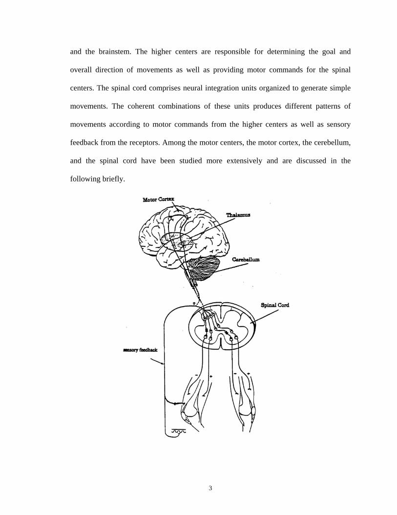
and the brainstem. The higher centers are responsible for determining the goal and

overall direction of movements as well as providing motor commands for the spinal

centers. The spinal cord comprises neural integration units organized to generate simple

movements. The coherent combinations of these units produces different patterns of

movements according to motor commands from the higher centers as well as sensory

feedback from the receptors. Among the motor centers, the motor cortex, the cerebellum,

and the spinal cord have been studied more extensively and are discussed in the

following briefly.

3

Fig. 1-1 A simplified biological structure of the human motor system. [Adapted from Schmidt (1978) page 176, and Kandel et al. (1991) page 280]

- The Motor Cortex:

Electrical stimulation of the precentral of the cerebral cortex, called the motor

cortex, generates movements. This suggests direct involvement of the motor cortex in the

control of movements. The experimental results show that the motor cortex is activated

50 ms prior to EMG (muscle) activity. This short period of time implies that the motor

cortex is one of the last sites in the brain activated before the movement begins. Thus, it

is involved in the execution of the movement rather than in its planning (Rosenbaum,

1991). Penfield and Rasmuseen (Kandel et al., 1991) found a motor map which relates

the neighboring points of the motor cortex to the neighboring parts of the musculature.

That is, specific areas of the motor cortex control specific parts of body. Some parts of

the human body, such as fingers and lips, correspond to relatively larger control sites in

the motor cortex indicating that these segments have a better capability for fine control

than the other segments.

Recent evidence by Georgopoulos and colleagues (Georgopoulos et al., 1986;

Georgopoulos et al., 1989; Georgopoulos, 1990) shows that the motor cortex activity is

probably related to two important control parameters of motion, that is, force and

direction. This finding suggests that while the muscle force is related to the discharge

frequency of “single neurons”, the direction and magnitude of the movement is

determined by a “population of neurons”.

4

- The Cerebellum:

The anatomy of the cerebellum is simpler and more regular than the other cortical

motor centers; thus, it has been studied more extensively. The cerebellum is believed to

be among the centers that have motor learning abilities, primarily due to the plasticity of

the Purkinje cells' (the main output cells of the cerebellum) synaptic junctions with the

granule cell parallel fibers. The strengths of these junctions are adjusted by the climbing

fibers carrying the movement errors (Ito, 1984). Although the cerebellum is not involved

in motor activities directly, it has a very important role for movement co-ordination as

well as for "long-term" and "short-term" predictions (Stein, 1986; Houk et al., 1996). It

receives rich sensory feedback information as well as a copy of the motor command

(called the efference1 copy) sent to the spinal cord; therefore, it is aware of what the

lower levels have to do and what is being done. Based on this, different models have

been suggested for the cerebellum: a comparator for detection of the movement error

(Stein, 1986), an internal model of the neuromusculoskeletal system (Miall et al., 1993),

and an adaptive filter (Fujita, 1982). More recently, Smith (1996) proposed the

cerebellum as a regulator for joint stiffness. The stiffness is adjusted through the

reciprocal inhibition or co-contraction of agonist-antagonist muscles.

-The Spinal Cord:

The spinal cord is not just a simple pathway for transmitting motor commands

and sensory information; it contains basic neural units for generating simple movements.

Although the synaptic connections between neurons in the spinal cord are genetically

5

fixed (that is, no synaptic plasticity), the spinal circuits can be adaptive. The neuron gain,

for example, may be adjusted by tonic or phasic command from a higher level, and is

assumed to be done by the Renshaw cells (Hemami and Stokes, 1983).

Examples of the basic spinal units are: reflexes, central pattern generators, and

servomechanisms. A reflex is a relatively stereotyped response to a specific sensory

stimulus. It may be simple such as the mono-synaptic stretch reflex or complex such as

scratching in animals. Spinal reflexes are important for protection of muscles, limbs, and

the body against sudden external disturbance, and for co-ordination of the relevant

muscles in different voluntary movements.

The central pattern generators (CPG) generate the required motor patterns for

rhythmic movements such as locomotion (Kandel et al., 1995). Grillner (1985) proposed

a CPG network for locomotion. The network has been constructed from individual and

coupled CPG units controlling limbs. An activation of the whole network by the higher

motor centers such as the brainstem generates locomotion and an activation of an

individual unit controls the movement of a joint (for example the knee) or a group of

muscles. By changing the arrangement of the units, the central nervous system can

generate different rhythmic movements. For example, the same units but with different

arrangement may be used in locomotion as well as scratching (Guyton, 1991).

1 Efferent information is referred to those being conveyed away from the CNS toward periphery. Afferent information is referred to those directed from periphery toward the CNS.

6

1.1.2 Sensory Feedback

The central nervous system is informed about body posture, results of movement,

and the environment through cutaneous receptors, proprioceptors (sometimes referred to

as kinesthesis), and the visual and vestibular systems. Cutaneous receptors are important

in connecting the body with the environment and objects, for example, foot contact in

walking. The proprioceptors are responsible for collecting information about the position

and movement of the limbs and reporting this information to the CNS. They include

muscle spindles (sensitive to muscle length and changes of length), the Golgi tendon

organs (sensitive to muscle tension) and joint receptors (sensitive to joint position). The

visual system provides information not only about the location and movement of other

objects in the environment but also about the position and movement of our own body

segments. The visual feedback is therefore very helpful for transformation between the

external and internal frames of reference (Hemami, 1985). The vestibular system

provides information about head movement, and it is important for the maintenance of

postural stability.

1.1.3 Motor Control Modes

One important attribute of the human motor control system is the ability to

perform a variety of movements under different environmental conditions. This implies

that the whole system is a complex system with multiple aspects. Most of the available

theories and hypotheses proposed in motor control have been based on the study of a

7

specific (usually simple) movement under constrained conditions. Thus, they address a

specific aspect of the system rather than its general aspect. The role of sensory

information in the control of movements has been a controversial subject for a century.

Schmidt (1988) pointed out two groups of scientists he referred as the “peripheralists”

and the “centralists”. The first group believed that the movements are controlled through

feedback mechanisms and emphasized the closed-loop behavior of the motor system. The

second group believed that the movements were controlled by the central motor

commands and emphasized the open-loop behavior of the motor system.

- Closed-Loop and Open-Loop Modes:

The closed-loop mode is based on finding and correcting the error between the

desired movement (reference) and the actual movement reported by sensory feedback.

The feedback information is also essential for learning new skills. Adams (1971)

proposed a closed-loop model for skill acquisition. In Adams’ model the reference of

correctness, the so-called “perceptual trace”, was formed by the sensory feedback over a

period of practice. The closed-loop control mode is necessary for accurate and slow

movements such as tracking a trajectory, moving at a constant velocity, or postural

control, but it is insufficient to explain fast movements. One reason is that the time

required for detecting and processing feedback information is about 150-200 ms

(Schmidt, 1988), while many rapid movements such as piano playing are carried out in

less than 50 ms. For the study of rapid and well-learned movements many researchers

have proposed open-loop models. Among these models, “motor program” and

“equilibrium point” models are of great importance and are discussed briefly.

8

- Motor Program:

Keele (1968, page 387) defined the motor program as “a set of muscle (motor)

commands that are structured before a movement sequence begins, and that allows the

sequence to be carried out uninfluenced by peripheral feedback”. Keele’s definition

emphasizes two points: the program is built up in advance and the movement is

performed with no feedback. These two features are the main differences between open-

loop and closed-loop models. Brooks (1986, page 7) stressed the hierarchical structure of

the motor program: “ Motor plans are made up of several programs that, in turn, consist

of coordinated, smaller learned subroutines called subprograms. These subprograms not

only encode actual muscle activity but also act as commands for the initiation of other

subprograms”. In 1975, a few years after Adams’ closed-loop theory, Schmidt (1988)

proposed the schema theory in which he emphasized the open-loop movements and

generalized motor program. The generalized motor programs are formed parametrically

for a class of movements. To perform a specific movement, the Central Nervous System

(CNS) only needs to set the values of the parameters in the motor program. The motor

programs at higher motor centers, therefore, can store an abstraction of the movements.

This decreases the mental effort required to determine the motor commands for

individual muscles. He also pointed out the role of the motor program in muscle synergy

and argued that the motor subprograms constrain groups of muscles to work together and

act functionally as a unit.

9

- Equilibrium Point Hypothesis:

The equilibrium point hypothesis is an essential theory in motor control

(Feldman, 1966, 1974, 1986; Bizzi et al., 1982, 1992; Hasan and Enoka, 1985; Flash,

1987; Latash, 1993). This theory suggests that the position of a joint is determined by the

mechanical balance between the muscles and the external load acting on the joint.

Movements are generated by a shift in the equilibrium point. Although the theory points

to an implicit feedback mechanism to keep the joint position at the equilibrium point,

there is no global feedback to the higher centers. A limitation of this theory is that the

mechanism by which the central nervous system changes the equilibrium point has not

been clearly described. That is, the roles of the higher motor centers in the brain in tuning

the equilibrium point and generating movement have not been specified. Furthermore, it

is not clear how a priori knowledge of the neuromusculoskeletal system and

environmental factors affect the control of the equilibrium point. These are addressed in

the model proposed in this thesis by use of a model predictive controller.

- Hierarchical Structure:

Hierarchical control structures have been suggested for human voluntary

movement by many researchers (Schmidt, 1978; Brooks, 1986; Schmidt, 1988;

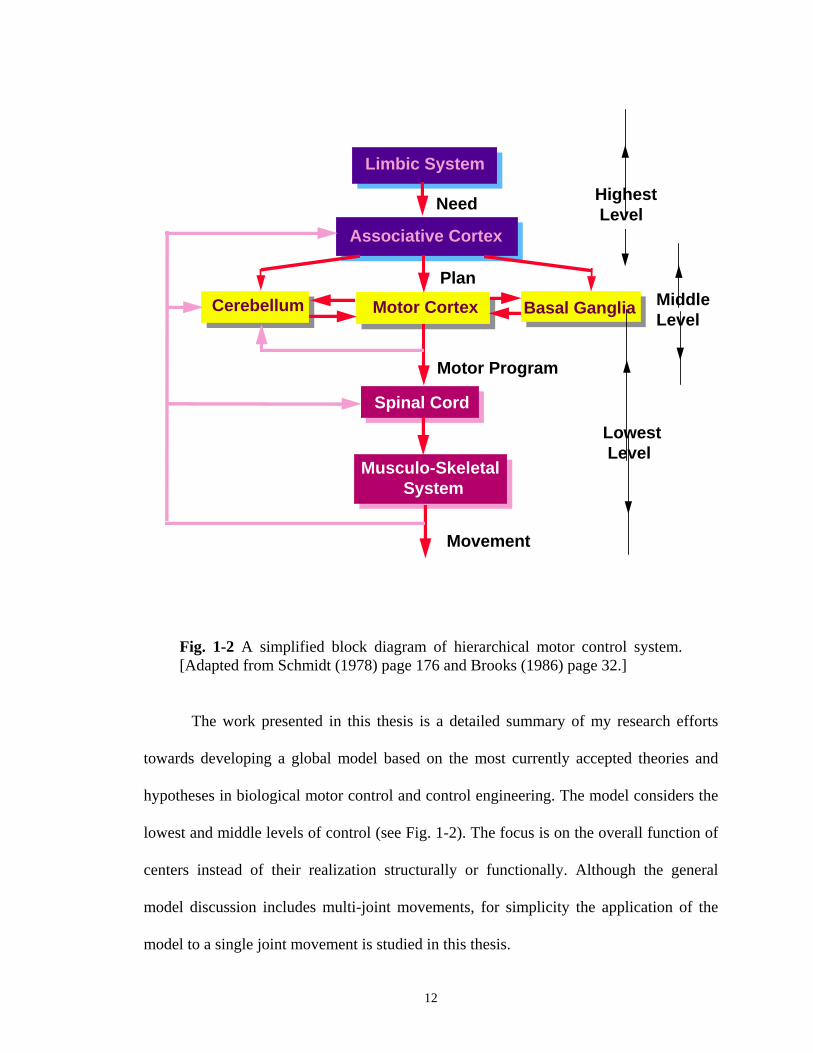
Carpenter, 1991; Latash, 1993; Kawato et al., 1987). A simplified functional three-level

control scheme is shown in Fig. 1-2. The "needs" and "demands" are felt by the limbic

system and are given to the associative cortex at the highest level. Based on previous

experience and feedback information received from lower levels and the external world,

the associative cortex selects the overall "plans" and "strategies". Then, it triggers the

10

motor cortex at the middle level to generate motor programs or motor instructions. The

cerebellum and basal ganglia, at the middle level, co-operate with the motor cortex and

the associative cortex to improve motor behavior. These programs are translated to the

muscles' “language” by the spinal cord at the lowest level of the control hierarchy. As

mentioned before, the spinal neural units such as reflexes perform simple movements and

co-operate in muscle synergies.

1.2 SCOPE OF THIS THESIS

For a comprehensive understanding of the motor control system, it is necessary to

have a global model. This model can be used also to test the function of motor

components under natural or pathological conditions. However, achieving such a global

model is a very difficult task. Most of the previous models deal with the modeling of the

musculoskeletal system and the spinal level of control. The main reason for this is that

there is much less data about the higher center function available than for the

musculoskeletal system due to the high degree of integration of these centers and the

many feedback pathways. The inputs and outputs of neural motor centers are also very

hard if not impossible to measure. This makes the identification task very difficult.

Moreover, the human motor system is an adaptive system and at present there is no

systematic approach to identify an adaptive system. The other reason is, to control a plant

(musculoskeletal system in this case), it is necessary to have adequate information about

it a priori. The more information that is available about the plant, the better the controller

can be designed.

11

Limbic System

Associative Cortex

Cerebellum Motor Cortex Basal Ganglia

Spinal Cord

Musculo-Skeletal System

Movement

Motor Program

Need

Plan

Highest Level

Lowest Level

MiddleLevel

Fig. 1-2 A simplified block diagram of hierarchical motor control system. [Adapted from Schmidt (1978) page 176 and Brooks (1986) page 32.]

The work presented in this thesis is a detailed summary of my research efforts

towards developing a global model based on the most currently accepted theories and

hypotheses in biological motor control and control engineering. The model considers the

lowest and middle levels of control (see Fig. 1-2). The focus is on the overall function of

centers instead of their realization structurally or functionally. Although the general

model discussion includes multi-joint movements, for simplicity the application of the

model to a single joint movement is studied in this thesis.

12

To develop a powerful motor control model, the model has to be able to deal with

the problematic control issues including transmitting and processing time delays, a

multivariable plant, an unstable plant, a non-minimum phase plant, operating constraints,

and external disturbances. The model also must be adaptive, robust, and able to operate

in open-loop (for ballistic movement) and closed-loop (for accurate movement or

learning a new movement) modes. No earlier control model has considered these factors

collectively. The model proposed in this thesis is based on three key factors: impedance

control as the control strategy, model predictive control as a model for higher motor

centers, and an external disturbance input for adding the environmental effects. The

model is called "Model Predictive Impedance Control (MPIC)". It is the first time that a

model predictive controller is suggested as a higher level controller for biological motor

control; however, the use of other types of model-based controllers with less generality in

motor control has been reported (see Chapter 2 for details).

1.3 OBJECTIVES OF THE THESIS

The main objective of this research was to combine and to unify the most

accepted theories available in the area of biological motor control and control

engineering to develop a model for a joint position and movement control. This model

could be a step toward achieving a global model. The model, called model predictive

impedance control, presents a unification of the following theories and strategies:

position/velocity control and impedance control strategies, equilibrium point hypothesis,

servomechanism theory, and optimization-based model predictive control algorithm.

13

The second objective was to provide a bridge for the gap between the equilibrium

point hypothesis and the higher motor centers which generate central commands. That is,

the roles of the higher motor centers in the brain in tuning the equilibrium point and

generating movement have not been specified. Furthermore, it is not clear how a priori

knowledge of the neuromusculoskeletal system and the environment affects the control of

the equilibrium point. These are addressed in the model proposed in this thesis by use of

a model predictive controller.

The specific objectives can be summarized as follows:

1- to develop the control system model,

2- to apply the model to different types of movements including a tracking

movement, a rhythmic movement, and an inverted pendulum model for walking,

3- to test the model’s sensitivity to plant model mismatching (robustness),

4- to identify the plant with a neural network.

As mentioned before, the results of this study can be used to better understand

human motor control and to design future experiments. They may also be useful in

control of artificial limbs (prostheses) for amputees or in functional neuromuscular

stimulation (FNS) to control paralyzed natural limbs with an artificial controller. A

limitation of the model for the latter applications is that the controller processing time is

too long for on-line control. It is expected, however, that with the on-going progress in

VLSI technology, manufacturing new and more powerful neural network chips, and

improving the available optimization algorithms, this limitation will be resolved in the

near future.

14

The model was simulated on a 486-PC computer. All the programs for model

simulation were written in MATLAB language (MathWorks, 1992). The identification

and neural network programs were written in FORTRAN language and performed on a

VAX machine so as to achieve higher speed.

Chapter 2 of this thesis discusses the impedance control strategy and the model

predictive control algorithm as the principles of the proposed model. The neural

identification of the neuromusculoskeletal system (the plant) is the subject of Chapter 3.

In the next chapter, the model predictive impedance control is described. Chapter 5 is

about the application of the model to three different types of movements and test of

model mismatching (robustness). Finally the summary and future directions are discussed

in Chapter 6.

15

CHAPTER 2- BASIS FOR MODEL PREDICTIVE IMPEDANCE CONTROL

Two key questions are to be answered in analysis or design of any control system:

what plant variables are controlled, and how these variables are controlled. Regarding the

biological motor control system, there are no definite answers for these questions due to

the system complexity and inadequate understanding of the system mechanism. In this

chapter the researchers' answers to these questions are briefly reviewed and the bases of

the MPIC are discussed. The first section deals with the first question and the second and

third sections deal with the second question.

2.1 IMPEDANCE CONTROL STRATEGY

Based on experimental results, and inspired from robotics and control engineering

studies, researchers have suggested the following muscle/joint parameters as the control

variables that may be used by the CNS to generate joint movements (Stein, 1982): force,

length, velocity, stiffness, viscosity, or a combination of the above variables. Stein

showed that the largest single group of researchers in motor control, 42 percent, believed

that more than one variable are controlled. He also predicted that all of the above

apparently different strategies could be different aspects of a single strategy in which

only one variable is controlled. In his commentary on Stein's prediction, Hoffer (1982)

suggested the mechanical impedance as the variable for a unified motor control scheme.

From this perspective, the other strategies are specific cases of the impedance control

strategy. Winters et al. (1988, page 1011) defined the impedance as: “the automatic

16

capability of the system to resist an applied load before voluntary intervention takes

place”. Joint impedance modulation is essential for postural stability as well as for

stabilizing an unstable load (Hogan, 1990).

Stiffness, static impedance, is defined as the ratio of change in force or torque to

change in length or angle. Muscle stiffness is a nonlinear function of muscle length,

muscle velocity, and input from higher neural centers. It consists of two parts: the active

part depending upon the output of motoneurons at the spinal cord, and the passive part

depending upon muscle elasticity. Joint stiffness is the sum of the individual stiffnesses

of the muscles acting on the joint. Thus tuning the joint stiffness is carried out by two

mechanisms: changing individual muscle stiffness through position receptors and a

closed loop circuit at the spinal level, and coordinating the opposing muscles by means of

co-contraction or reciprocal contraction of agonist and antagonist muscles coordinated by

the higher neural centers (Winters et al., 1988).

The discussion is continued by a review on the control of stiffness (static

impedance) which has been studied extensively.

2.1.1 Stiffness Control Strategy and Equilibrium Point Hypothesis

Stiffness control is the primary version of impedance control for control of

posture and movement in both biological motor control (Feldman, 1966, 1974, 1986;

Bizzi et al., 1982, 1992; Hogan, 1984a; Houk, 1979; Flash, 1987; Hasan, 1986,

Towhidkhah et al., 1993) and robotics ( Hogan, 1984b, 1985a, and 1985b; Lee et al.,

1994). Most of the biological studies have dealt with the theoretical development of the

strategy, the spinal neural circuits and the reflexes involved, and the experimental

evidence. Less attention has been given to the role of the motor centers in the brain (such

as the motor cortex and the cerebellum) to realize this strategy. Most recently, Smith

17

(1996) discussed the role of the cerebellum in tuning joint stiffness by modulating the co-

contraction of agonist and antagonist muscles.

Joint stiffness plays an important role not only in increasing the joint resistance to

an external disturbance but also in initiating movements without disturbance (Hasan,

1986). The joint impedance is suggested for fast compensation of external disturbance

effects where the reaction is too fast to have been carried out through the cortical loop.

Hogan (1984b, 1985a) showed the advantage of stiffness control in contact of the limb

with environment and tool usage. Abul Haj and Hogan (1987) applied the stiffness

control to improve the poor performance of cybernetic prostheses.

In the biological motor control literature, the idea of stiffness control has a very

close relationship with the equilibrium point hypothesis (EPH) which was first proposed

by Feldman (1966) for control of posture, and was then extended to control of voluntary

movements (Feldman, 1986; Bizzi et al., 1982, 1992; Flash, 1987, Flanagon et al., 1993).

According to this hypothesis, a voluntary movement is accomplished as a sequence of

shifts in the joint equilibrium point. The equilibrium point concept is a classical approach

in nonlinear control systems including autonomic control systems of the human body

such as regulation of body temperature and blood glucose (Milhorn, 1966). In these

systems, in contrast to classical linear control systems, the set point is usually hidden,

that is, there is no explicit desired output(s) (for example temperature of 37°C) defined

by other centers in the body. The desired output is determined by the stable crossing

point of the characteristics of the elements and subsystems constructing the system as

well as the characteristic of the environment. This crossing point is referred to as the

"equilibrium point". Any change in environmental or system parameters changes the

equilibrium point which is compensated by adjusting other parameters or characteristics.

Thus it points to an adaptive mechanism.

Fig. 2-1 indicates the idea of stiffness control in which a muscle is assumed to be

an active adjustable spring whose stiffness (Bizzi's α model (Feldman, 1986)), or

18

equilibrium position (Feldman's λ model (Feldman, 1986)), is tuned by the CNS. A

combination of λ and α models has also been proposed (Hasan, 1986; McIntyre and

Bizzi, 1993). Although the forces generated by the agonist muscles are in opposite

directions, the stiffnesses of these muscles are additive. The spring-like behavior of

muscles and joint can also be explained based on the force-length or torque-angle

characteristic of an agonist-antagonist pair and their net characteristic (see Fig. 2-2). The

crossover of the net characteristic with the horizontal axis (β) is called the slack angle,

and it shows the equilibrium position (or desired position) of the joint when there is no

external disturbance. The value of β is adjusted by reciprocal contraction of opposing

muscles. The slope of the net characteristic (σ) shows the joint stiffness, and it is adjusted

by co-contraction of opposing muscles. In order to change the joint position from the

initial position, β1 in Fig. 2-3, to a new position, β2, it is sufficient that the CNS adjusts

the characteristics (stiffnesses) of agonist and antagonist muscle such that the net

characteristic (assumed here to be a line for simplicity) shifts from β1 to β2. In this case,

β2 would be the new equilibrium position. The torque generated by the muscles is

proportional to the difference between the equilibrium (desired position) and the current

position.

19

Fig. 2-1 Principle of the stiffness control strategy. [Adapted from Kandel et al. (1991) page 561].

Fig. 2-2 The basis of equilibrium point hypothesis. σ is the incremental joint stiffness and β is the slack angle.

20

Torque

Angle1 2

θi=β1 θf=β2

Fig. 2-3 A new equilibrium position as a shift in net characteristic. Point 1 is the initial position and point 2 is the final position.

Torque

Angle1

2

θi=β1 θf=β2

βv

Td

σ

Fig 2-4 The effect of disturbance on change of equilibrium position. βv is the virtual equilibrium point. σ is the joint stiffness. θi is initial and θf is the desired positions. Td represents the external disturbance.

21

If the external disturbance is not zero, the equilibrium position will not be

specified by β any more, but it will be determined by the values of the final desired

position, θf, and the external disturbance, Td, that is, point 2 in Fig. 2-4. The line with a

slope of σ passing through point 2 crosses over the angle axis at a point called the virtual

equilibrium point, βv. Thus, the system with disturbance Td and desired angle θf,

statically can be equivalent to the same system when Td equals zero and the desired

angle is βv. It is easy to show that:

βv = θf - Td/σ. (2.1)

2.1.2 Impedance Control Strategy and Generalization of EPH

Although the stiffness may be sufficient to analyze slow and quasi-static

movements, it is not sufficient for the analysis of faster movements. To generalize the

model for slow and fast movement analysis, viscosity (dynamic impedance) was added to

later versions of the impedance control and EPH (Feldman, 1986; Flash, 1987; McIntyre

and Bizzi 1993). In this case, the concept of EPH is generalized by applying a 3-

dimensional torque-angle-angular velocity characteristic of the joint rather than the 2-

dimensional torque-angle characteristic (Fig. 2-5) (Brooks, 1986). The net joint

characteristic, in this instance, would be a 3-dimensional surface, Fig. 2-6, whose

intersection with the load-disturbance characteristic specifies the equilibrium point Q.

The position of Q is adjusted by changing muscle and joint characteristics. The

geometrical projections of the equilibrium point on angle and angular velocity axes are

shown by β and β.

respectively, and its height represents the required torque to

compensate the external disturbance effect. The incremental slope of the net

characteristic with respect to joint angle is shown by σ, and the slope of net characteristic

with respect to joint angular velocity is shown by b, that is:

22

σ =δ(Τorque)

Angle)δ( (2.2)

b Torque=

δδ

( )(Angular Velocity)

(2.3)

Assuming P as the current operating point relating to the actual joint position and joint

velocity, the torque generated by the muscles is proportional to the PQ (error) vector.

This mechanism, that is, correction of the difference between the desired point (Q) and

the actual point (P), implicitly indicates a feedback mechanism which is the basis for the

well-known advantage of EPH for fast load compensation. For a constant desired joint

position, β.

is zero, and the equilibrium point is called the "static equilibrium point". But

for a desired joint movement, β and β.

are time variables, and there is a trajectory for Q.

Thus, the equilibrium point in this case is referred to as the "dynamic equilibrium point".

Fig. 2-5 3-D active muscles characteristic (Adapted from Brooks, 1986).

23

Fig. 2-6 Principle of the 3-D equilibrium point hypothesis. The three dimensional surface is the new net characteristic of antagonist muscles. P represents the current output state, and Q represents the desired output state or equilibrium point. The solid line represents the load-disturbance characteristic which intersects the net muscle characteristic at point Q. The vector P to Q represents the error which generates the torque required to establish the new equilibrium point. β is the slack angle, and β

. is the slack angular velocity.

As mentioned before, the joint (muscle) impedance control strategy includes

angle (length), angular velocity (velocity), and torque (force) control strategies. The slack

angle and angular velocity, β and β.

, in fact, represent the control of angle and angular

velocity. In postural control (isometric condition) the stiffness is proportional to the

force. Thus, stiffness control represents force control. Highly accurate movements, such

as these needed in microsurgery, can be performed by increasing co-contraction (high

stiffness mode), and low accurate movements such as throwing a ball can be performed

by decreasing co-contraction (low stiffness mode).

The second question is the problem of controller design and is addressed in the

next two sections.

24

2.2 OPTIMIZATION-BASED STRATEGIES

A widely-used theoretical approach for finding the control variables is an

optimization technique. The goal of movement is modeled as a mathematical scalar

function referred to as a “performance index”, “performance criterion”, “cost function”,

“objective function”, or “penalty function”. The aim is to determine the control variables

to minimize or maximize this function. In addition to the cost function, the movement

pattern depends on the system dynamics, internal and external constraints, and the

optimization procedure being used. Examples of internal constraints are limitations on

ranges of joint movement (due to cartilages and ligaments) (Hemami, 1985), of

maximum muscular force, and of rate of change of force (Stein et al., 1986). Some of the

movement objectives such as time or distance of movement may also be assumed as

constraints (Nelson, 1983). Constraints can be useful for decreasing the degrees of

freedom and increasing muscle synergy which allow application of a simpler controller.

For a simple linear system, optimization results in a closed form analytical

relationship between system parameters and the control variables, but for high-order

linear systems or nonlinear systems, numerical techniques are usually necessary. The

numerical techniques may be divided into two major groups: gradient-based and random

search methods. The problem with the gradient methods is that there is no guarantee of

convergence or of finding the global minimum. The problem with random search

methods is that they require extensive computational efforts.

Recently, the Genetic Algorithms (GAs) have been suggested (Holland, 1975;

Goldberg, 1989; Vose, 1991; Osyczka and Kundu, 1995) for finding the global minimum

with less effort. It is a "directed" random search method inspired from natural evolution.

The GA is based on variation, selection, and inheritance (Forrest, 1993). The information

is represented in the form of chromosomes or strings (typically binary strings). The

strings are constructed from elementary particles referred to as genes (0 and 1 in binary

25

strings). A population of strings are applied for fitness evaluation. The strings with high

fitness values (good individuals) are selected to produce a new generation (offspring)

using mutation and/or crossover approaches. The average fitness of the population is

improved over many generations. The efficiency of the GA depends on the selection of a

proper form for information representation, the fitness function, and the interdependency

among the genes called epistasis. For low epistasis (almost linear) systems, gradient

methods; for mild epistasis (mild nonlinear) systems, the GAs; and for high epistasis

(high nonlinear) systems, random search methods were suggested by Davidor (1991).

As mentioned before, defining the cost function plays a key role in optimization.

The criteria functions applied in biological motor control have been functions of kinetic

(torque) and kinematic (angle, velocity, acceleration, and jerk) parameters. Nelson (1983)

applied different movement criteria to model rhythmic movements. The criteria included

time, maximum force, peak velocity, energy (squared force), and jerk (the change of

acceleration). For minimum-time movement the controller was found to be bang-bang,

that is, biphasic muscular activation. Each muscle must be innervated maximally over the

entire movement. A bang-bang type controller has been also reported by Oguztoreli and

Stein (1983), Zangemeister et al. (1981), Stein et al. (1986), and Seif-Naraghi and

Winters (1990). The bang-bang switching frequency, that is, the number of phases in the

control signal, is a function of the musculoskeletal system complexity. For a linear

model, this frequency is proportional to the number of negative real poles of the system

(Seif-Naraghi and Winters, 1990).

Human movements, however, have often been characterized to be graceful and

smooth. An arm movement path between two points is close to a straight line with a bell

shape velocity profile. To achieve maximum smoothness, Hogan (1984c) proposed a

"minimum-jerk model" for single joint movement. This model was extended to multi-

joint movements by Flash and Hogan (1985). The form of output trajectory for the

minimum-jerk model is a sigmoid type with a bell-shape velocity profile which is

26

smoother than that of a bang-bang controller. Hasan (1986) found similar results by using

subject "effort" as the criterion function. In Hasan's model, effort was mathematically

defined as a time integral of squared sum of velocity and jerk product by joint stiffness

(see the equation 4.3). To consider dynamic terms, Uno et al. (1989) suggested a

"minimum torque-change model". This model is identical to the minimum jerk model for

linear systems. Stein et al. (1986) showed that the limitations of force output and time

constants blur the distinction between different criteria strategies. The smoothness of

movement, thus, may arise from neuromuscular nonlinearities and muscle low pass

filtering effects rather than jerk necessarily being minimized. Seif-Naraghi and Winters

(1990) mentioned that minimizing jerk tends to a "pull-pull" strategy which requires a

higher degree of muscle co-contraction which in turn is not efficient. They proposed that

adding a neuromuscular penalty (that is, neural effort, muscle stress, and muscle

dissipation) to the criterion function often shortens the convergence time and moderates

the movements.

2.3 MODEL-BASED STRATEGIES

In parallel with control theory development, model-based control schemes have

been applied in biological motor control modeling. These control schemes generally

contain a form of dynamic model, either an inverse model or a forward model (internal

model) representing dynamic information of the neuromusculoskeletal system. A

reference model also has been proposed to visualize the desired or acceptable system

response. The human motor system has been hypothesized to include such a dynamic

model (Kawato et al., 1987; Neilson et al., 1988; Miall et al., 1993; Hirayama et al.

1993; and Shadmehr and Mussa-Ivaldi, 1994). This model is achieved through a learning

process. The experimental bases for this theory are: first, many fast movements such as

playing a piano and typing are too fast to be performed through the delayed feedback

27

mechanism. An internal model in this case could replace the delayed feedback

mechanism, and the output of the plant model used for control instead of the plant output

(afferent information). Second, prediction is a well-known feature of the human motor

system. Acting as a predictor, the dynamic model can predict where the movement is

going and help the controller to provide a corrective control signal in advance. This is a

key point in the model predictive control algorithm discussed in the next section.

The cerebellum has been recognized as one of the important motor centers

involved in motor learning (Ito, 1970, and 1984; Houk et al., 1996) and in providing

predictive information (Stein, 1986). It also receives large amounts of information about

the result of movements and the environment from sensory receptors as well as an

efferent copy of the motor command descending to the spinal cord. Some researchers (for

example Ito, 1970; Kawato et al., 1987; Miall et al. 1993), therefore, have suggested the

cerebellum may include a form of internal model.

Direct inverse dynamic modeling is attractive for its direct implication as a

controller (the ideal controller is inverse dynamic of the plant). However, it is not goal-

directed (Jordan and Rumelhart, 1992), and, for a non-one-to-one nonlinear system such

as the biological motor system, the desired inverse dynamics of the system may not be

achieved. In contrast, a forward model is goal-directed and biologically more feasible,

but it is not directly applicable for control. Jordan and Rumelhart (1992) suggested a

combination of forward and inverse models to resolve these problems. The forward

model first identifies the system, then, the inverse dynamic model, that is, the controller,

is trained by using the forward model information. They showed that an acceptable

inverse model can be achieved even with an approximate forward model. Kawato et al.

(1987) proposed an alternative method, feedback-error-learning, to find the inverse

model. Their model is based on simultaneous control and learning, and employs a

feedback controller and a feedforward (inverse dynamic) neural controller. The inverse

model is trained through feedback torque instead of the desired output. In the early stages

28

of learning, the error correction and system stability are provided by the feedback

controller. Once the feedforward controller learns the system inverse dynamics, the

feedback signal tends to zero, and the control mechanism is switched from closed-loop to

open-loop which allows performing the action faster. A problem with this model is that a

zero feedback signal does not necessarily mean that the feedforward controller has

learned the system inverse dynamics, but it may have learned the steady state inverse of

the system. In addition, as mentioned by Kawato (1990), convergence is only achieved if

the feedback gains are sufficiently small that the system responds very slowly.

These models have not taken into consideration the system time delays resulting

from neural processing and signal transmission. Time delays are problematic factors in

feedback control systems causing system instability and leading to low gain and slow

system response. The delay reported for proprioceptive feedback is 100-150 ms and for

visual feedback about 200 ms (Hogan, 1985b, Miall et al. 1993). Most recently, Miall

et al. (1993) suggested a modified version of the Smith predictor as a likely model for the

cerebellum. The Smith predictor effectively shifts the time delay from inside the

feedback loop to outside the feedback and allows a higher loop gain and thus a faster

response.

Similarly, the MPC algorithm uses a form of forward model to cope with the

system time delays. However, the MPC algorithm is also a good candidate for non-

minimum phase or unstable systems (Clarke et al., 1987a; Demircioglu and Gawthrop,

1991), where most of the above models fail. The inverse dynamic controllers have

serious difficulty1 when dealing with these types of systems. In the impedance control

strategy, for example, if the joint stiffness (σ) is negative, the system will be non-

minimum phase, and its inverse results in an unstable controller. Moreover, many joint

movements may be modeled as unstable systems. For example, an inverted pendulum 1 The plant or inverse dynamic (feedforward) controller is unstable for an unstable or a non-minimum phase system, respectively. Because no controller is perfect, the net system (that is, the plant plus controller), therefore, would be unstable.

29

model is used to model human walking, head movement, or trunk movement. Thus a

motor control model is required to be applicable to such complex systems as well. In

contrast to conventional internal models and the Smith predictor approaches, the MPC

algorithm determines the control variables using optimization techniques. This leads the

controller to check the movement trajectory in advance and to satisfy operating

constraints. The MPC algorithm is discussed in the next section in more detail.

2.4 MODEL PREDICTIVE CONTROL ALGORITHM

Model predictive control was first proposed by engineers in industry in the late

1970s (Garcia et al., 1989), and it has been developed subsequently by academic

investigators (Clarke et al., 1987a and 1987b) for difficult-to-control systems such as

those including time delays, nonlinearities, operating constraints, multiple variables, non-

minimum phase zeros, and/or unstable poles. MPC generates control actions based on the

output prediction of the system to be controlled and optimization techniques. For linear

systems, convolution models, that is, the step response or the impulse response, are used.

These models may be obtained experimentally. The advantage of applying the step or

impulse response model is that it can be utilized for those systems that cannot be modeled

in the form of a simple parametric transfer function such as for first order or second order

systems; however, the cost is an increased number of parameters and computational

effort.

The basic idea of MPC is shown in Fig. 2-7. The predicted error is computed for

the future as the difference between the desired trajectory θd and the predicted trajectory

θp. The criterion function J is usually reestablished as a quadratic function of this error

and the control effort. For a single input single output system, the criterion function may

be written as:

30

. (2.4) J q t k t k r t kk

M

k

P

( ) { [ ( ) ( )] } { [ ( )] }∆ ∆β θ θ β= + − + + + −==∑∑ k kd p

2 2

11

1

∆β represents the control signal (or simply called control) deviations, and qk and rk are

weighting factors showing the importance of variables. P is called the prediction horizon,

and it refers to the time duration in which the output of the model is studied and used in

optimization. M is called the control horizon, and it refers to the number of future control

signal changes which are applied to the model to produce the predicted trajectory. θp is

determined by the dynamical models of the system and disturbance based on past,

present, and future control signal values as well as the estimation of the unmeasurable

disturbance, d. A simple estimation for d is obtained by computing the difference

between the system measured output, θm, and the model (predicted) output at the present

time and assuming that it is constant during the prediction horizon. The results of the

optimization are the optimized control signal values. Although the control values are

computed for the whole control horizon, only the first sample of the control values is

given to the system, and the optimization procedure is then repeated in the next sampling

period to find the next control values. The reasons for this are the system uncertainties

and the model imperfection.

31

Fig. 2-7 The principle of model predictive control. The three dimensional surface is the new net characteristic of antagonist muscles. P represents the current output state, and Q represents the desired output state or equilibrium point. The solid line represents the load-disturbance characteristic which intersects the net muscle characteristic at point Q. The vector for P to Q represents the error which generates the torque required to establish the new equilibrium point. β is the slack angle, and β

. is the slack angular velocity.

For the unconstrained linear system the optimization problem is easily solved by

using standard linear least squares error minimization which results in a linear time-

invariant controller. In the presence of linear constraints, a linear programming or a

quadratic programming technique is applied for a linear or a quadratic criterion function,

respectively. In comparison to linear programming, the controller suggested by the

quadratic programming strategy is easier to tune due to weighting factors in the quadratic

function, and usually provides a smoother response. However, its computational effort is

about four or five times longer than that for the linear programming controller (Seborg et

al., 1989). The optimization procedure for nonlinear systems is typically referred to as

the nonlinear programming problem for which there is no general solution. However,

32

some case-oriented solutions have been applied based on local linearization of the system

and/or approximation of the criteria functions with quadratic functions.

In the MPC algorithm, the prediction and control horizons are tuning factors. The

prediction horizon should be large enough to accommodate the system transient

dynamics. Increasing the value of P increases the system stability and moderates the

control signals; however, it also increases computing time (Seborg et al., 1989). M is also

an important design parameter. For a simple system M=1 has been found to be

acceptable, but for an unstable or poorly stable system it has been suggested that the

value of M should be greater than the number of unstable or highly-oscillatory poles

(Clarke et al., 1987a).

An important advantage of MPC is that it presents a multi-step prediction which

anticipates where the system is headed if the controls are applied, and in the case of

observing undesirable behavior of the plant or violating the operating constraints, the

recursive optimization algorithm improves the control signals.

2.5 SUMMARY

The principles of model predictive impedance control were discussed and the

related motor control models were briefly reviewed in this chapter. Model predictive

impedance control is based on three factors: impedance control strategy (or EPH),

optimization, and the MPC. The advantages of tuning joint impedance are as follows.

First, impedance control is a generalized strategy and other control strategies such as

position, velocity, torque, stiffness, and viscosity control strategies may be considered as

special cases of impedance control. Low stiffness (low degree of co-contraction), for

example, represents force control and high stiffness (high degree of co-contraction)

represents position control (Hoffer, 1982; Hogan, 1984b). Impedance control is also a

unique treatment for control of both posture and movements (Hogan, 1984b, and 1985c).

33

Second, impedance tuning is an effective method in interaction between a limb and other

limb or environment including stable contact task (Hogan, 1990) and tool usage (Abul-

Haj and Hogan, 1990). Third, impedance control can explain the fast compensation for

abrupt external disturbance which is too fast to be performed through the cortical loop

(Hogan, 1985c). Joint impedance modulation is also essential for postural stability as

well as for stabilizing an unstable load (Hogan, 1990). Fourth, there is increasingly

experimental support for stiffness and impedance control in biology and robotics.

The human motor control system is characterized as a complex learning and

predictive control system. Skilled movements are achieved in a learning process. The

more one practices, the better is the performance and the closer is the movement to the

optimal movement. The optimization technique, thus, points to the learning ability of the

motor system. A problem with optimization techniques is that different criteria may result

in similar responses. This makes it difficult to specify the criteria that may be used by the

CNS in natural movements. However, optimization has been recognized as a very

powerful technique to determine the control variables in biological motor control

research (Hogan and Winters 1990; Zajac and Winters, 1990). The CNS probably applies

different criteria to perform different movements and under different environmental

conditions (Oguztoreli and Stein, 1983). For fast movements, for example, minimizing

movement time seems reasonable, and for accurate movements, minimizing the output

error seems to be essential. Generalized forms of criteria have been suggested by some

investigators in motor control. A generalized criterion may contain a weighted

summation of subcriteria such as time movement, energy, output (or states) error(s), jerk

or neuromuscular effort. (Seif-Naraghi and Winters, 1990). Depending on the nature of

the movement the weighting factors are adjusted by the CNS. For instance, the speed-

accuracy trade-off (Schmidt, 1988) can be explained by adjusting the weighting factors of

time of movement and output error. Finding a suitable cost function and weighting

factors for a specific movement is not a trivial task and is out of the scope of this thesis.

34

The higher level controller proposed for the motor control scheme has to be able

to deal with systems with the following characteristics: multiple variables, time delay,

non-minimum phase zeros, unstable poles, operating constraints, and nonlinearities. It is

also necessary that the controller considers the external disturbance and can operate in

open-loop (ballistic movements) and closed loop modes. Being based on optimization,

MPC provides more generality regarding the above factors than the previous model-

based schemes suggested in motor control. Although the discussion about the motor

control scheme (Chapter 4) is easily extendable to multi joint movements, the application

of the model to a single joint movement with no constraint is investigated in this thesis.

MPC has shown its excellent performance in the control of a multi variables nonlinear

process (Ashobi, 1995).

35

CHAPTER 3- IDENTIFICATION OF THE NEUROMUSCLOSKELETAL SYSTEM USING NEURAL NETWORKS

As discussed in Chapter 2, model-based control strategies, including MPC, apply

the representation of the neuromusculoskeletal information in the form of a dynamic

model, for example, an internal model. This model is achieved through a learning process

and is used to predict the movement in advance and to design the controller. The

objective of this chapter is to propose a few recurrent neural network structures as

possible candidates for learning the dynamics of the knee joint and external disturbance,

rather than to present a complete investigation on different neural network models or

learning algorithms. Neural networks learn from examples, generalize the results, and

process the input information in parallel. It has been proven that any nonlinear function

can be estimated by multi-layer feedforward neural networks (Hornik et al., 1989; Hunt

and Sbarbaro, 1992). Neural networks have shown excellent performance in the modeling

of dynamic systems (Narendra and Parthasarathy, 1990). The features of neural networks

make them attractive for many information processing applications including pattern

recognition and nonlinear system identification. In this chapter, five recurrent neural

networks are investigated for their ability to model the neuromusculoskeletal system.

36

3.1 NEURAL NETWORK BACKGROUND

A neural network is an integration of highly interconnected cells called

“neurons”. A biological neuron (Fig. 3-1a) contains many dendrites, a soma, a nucleus,

and an axon with several branches. The neural activations generated by either sensory

receptors or other neurons are input to the neuron through synaptic junctions. These

activations may have excitatory (positive) or inhibitory (negative) effects on the neuron.

The importance of input activations are specified by synaptic weights which are

adjustable in some types of neurons. This synaptic plasticity has been proposed to be the

basis for biological long term memory and learning ability. Once the net input activation

of the neuron meets a threshold the neuron will fire at a rate that is proportional to the net

input activation. Similarly, an artificial neuron (Fig. 3-1b) contains synaptic weights, a

summer, a threshold, a nonlinear (activation) function, and an output. The output is a

nonlinear function of the weighted inputs summation, that is:

(3.1) y wf h hh 1

Nin

==∑[ ( u )]

where y is the neuron output, f is the nonlinear function (typically sigmoid), Nin the

number of inputs, wh the hth synaptic weight, and uh the hth input.

37

Axon

Dendrite

Synaptic Junctions

Nucleus

Soma

(a)

ΣΣNeuron

Nonlinearity

Inputs

Output

Synaptic Weights

(b)

Fig. 3-1 a) A biological neuron. b) An engineering model of a neuron.

38

Inputs Neuron

Desired Output

Adjustment Mechanism

Error

(a)

Inputs Neuron

Output

Adjustment Mechanism

(b)

Fig. 3-2 Learning methods: a) supervised method, b) unsupervised method.

The synaptic weights are adjusted during training of the neural network. Two

methods of learning are widely used: supervised and unsupervised methods (see Fig. 3-

2). In the supervised method, the desired output is determined by a “teacher”. The error

39

between the neuron output and the desired output is computed and is used to adjust the

weights. In the unsupervised method, there is no teacher, and the weights are adjusted

based on some sense of relationship between the inputs, or between inputs and output.

The biological evidence suggests that both supervised and unsupervised learning

mechanisms are likely employed by the central nervous system in order to adjust the

biological neural synaptic junctions. One method for the unsupervised learning

mechanism was suggested by Hebb (1949). In Hebbian learning, the correlation

(coincidency) between the excitation of the neuron output and a neuron input increases

the synaptic weight related to that input. A second unsupervised method is based on the

well-known Pavlovian experiment and is called "conditional learning". In this method the

correlation (coincidency) of two inputs determines the changes of the synaptic weights

related to those inputs. In conditional learning, the repeated coincidency of two events

(two inputs), called unconditional and conditional stimuli, causes the same response of

the unconditional event (input) to be generated by the conditional event (input).

Biological evidence for supervised learning was proposed by Ito (1970 and 1984).

He showed that the synaptic junctions of the Purkinje cells with the parallel fibers, in the

cerebellum, can be modified according to the error signals being propagated by the

climbing fibers. This plasticity is a possible basis for the cerebellar motor learning and

program storing. Ito suggested this mechanism for control of eye movement through the

flocculo-vestibulo-occular reflex loop. Once the position of eye does not match the

desired position, the climbing fibers (teaching lines) report the error to the flocculus to

modify synaptic coefficients. When the learning is complete, the error becomes zero.

40

3.2 NEURAL NETWORK MODELING

The static neural network (neural network with no input or output histories) has

been successful in pattern recognition (static identification) applications, but they are

unable to emulate dynamic systems. For dynamic system identification, a dynamic neural

network has to be applied. Dynamic networks may be realized by adding tapped delay

lines to multi-layer neural networks (Fig. 3-3). The histories of the inputs and outputs of

the system are introduced to the network through the tapped delay lines. Inspired from

traditional ARMA (Auto-Regressive Moving Average) filters, this structure has been

widely applied in modeling nonlinear systems. A limitation of this structure is that it is

useful primarily for those systems whose states can be extracted simply from the histories

of the inputs and the outputs of the system. A more suitable structure for dynamic neural

networks which obviates this limitation is a recurrent neural network such as the fully

recurrent Hopfield network. This dynamic network is very powerful and can be applied

in types of problems which cannot be handled by more standard control formulations.

Therefore, it is a suitable candidate for modeling of complex systems such as the

neuromuscloskeletal system. Recurrent neural networks can identify a nonlinear system

using fewer number of neurons compared to their feedforward counterparts; they provide

better generalization as well. The costs for these advantages are a more complex learning

algorithm, an extensive computational effort, and slower convergence. Modified versions

of fully recurrent neural networks may produce simpler structure, less computing time,

and faster convergence (Ashobi et al., 1995).

41

D

D

D

D

D

D

D

Inputx(n)

x(n-1)

x(n-2)

x(n-3)

y(n)

y(n-1)

y(n-2)

y(n-3)

Output

Time delay

Fig. 3-3 Tapped delay lines dynamic neural network.

In addition to the network structure, the learning algorithm plays a significant role

in dynamic behavior of a neural network. Recurrent networks with the same structure can

generate different dynamic behavior due to the use of different learning algorithms. The

simplest gradient-based method for training a recurrent neural network is the "back-

propagation-through-time" algorithm. This method unfolds the network through time,

that is, it replaces a one-layer recurrent network with a multi-layer feedforward neural

network that can be trained by the ordinary back propagation algorithm. The

disadvantages of this algorithm are: 1) it needs a model of the external environment, or it

should be used in a noise free system; and 2) for continual operation, it needs a lot of

42

memory; therefore, it is not useful for on-line identification. For on-line applications a

"real-time recurrent learning" algorithm can be applied. This algorithm is also based on

gradient method learning. One problem with the above algorithms is converging to local

minima. As mentioned in Chapter 2, using random search-based learning algorithms such

as the genetic algorithm may be useful in finding the global minimum. For noise-free

systems it is possible to use the states and the output of the system (if they are accessible)

instead of the states and the output of the neural model in the computation of the

gradient. This substitution removes the recurrent feedback virtually and allows the use of

less complex learning algorithms. This model was called the "series-parallel" model by

Narendra (Narendra and Parthasarathy, 1990). Another advantage of the series-parallel

model is that it is globally stable (Narendra, 1990).

3.3 MODELING THE NEUROMUSCULOSKELETAL SYSTEM

Figs. 3-4 and 3-5 show the Hopfield network and four other architectures of

recurrent networks chosen as candidates for identification of the neuromusculoskeletal

system (see Ashobi, 1995 and Towhidkhah et al., 1994a for more details). In the fully

recurrent Hopfield network (Hopfield, 1982), network a, each neuron (unit) receives a

delayed output from every neuron. All neurons receive the input signal(s) including a

constant bias input. Only the output neuron(s) receive the teaching signal(s). Each neural

unit performs a summation plus a nonlinear activation function. Networks b, c, d, and e

can be considered as modified versions of the Hopfield network, as follows. In the state

feedback network, network b, there are no feedback paths from the output neurons and

43

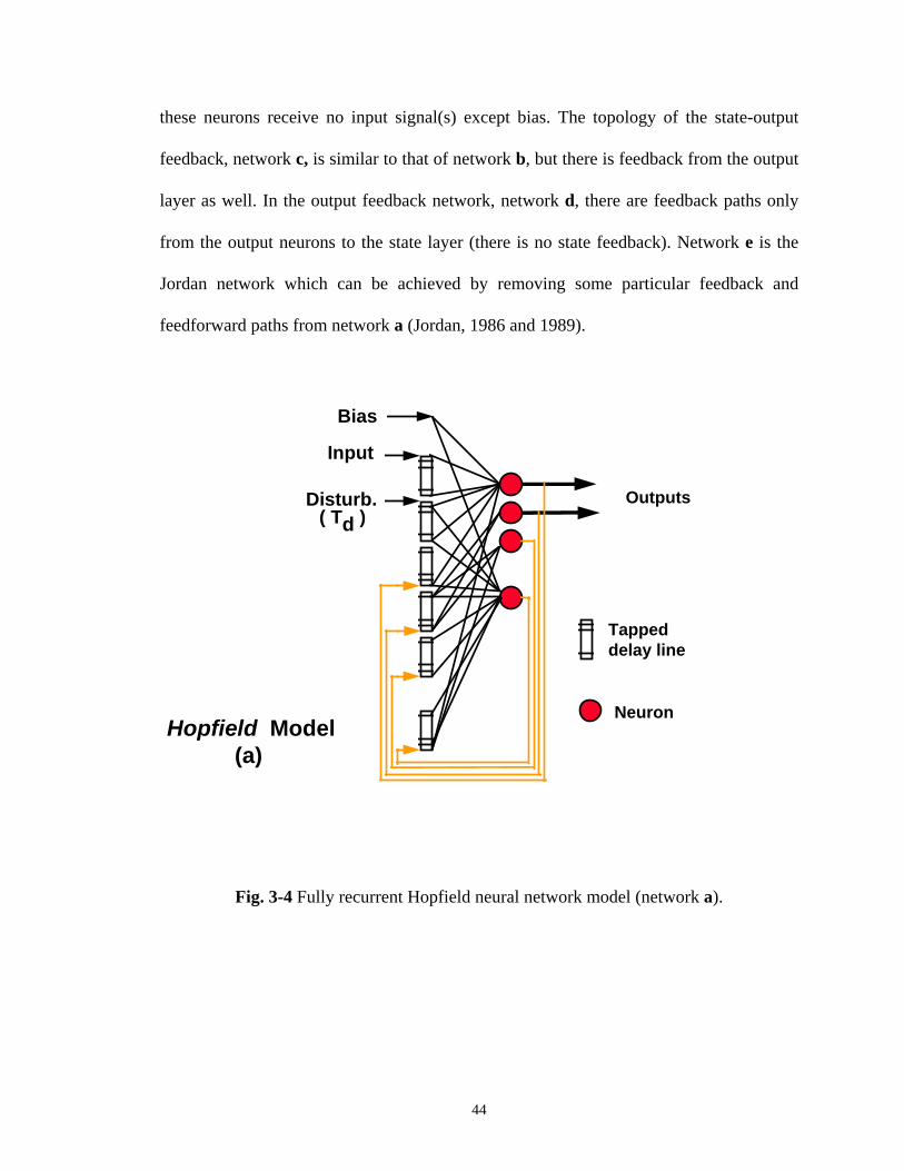
these neurons receive no input signal(s) except bias. The topology of the state-output

feedback, network c, is similar to that of network b, but there is feedback from the output

layer as well. In the output feedback network, network d, there are feedback paths only

from the output neurons to the state layer (there is no state feedback). Network e is the

Jordan network which can be achieved by removing some particular feedback and

feedforward paths from network a (Jordan, 1986 and 1989).

Hopfield Model(a)

Bias

Outputs

Tapped delay line

Input

Disturb.( Td )

Neuron

Fig. 3-4 Fully recurrent Hopfield neural network model (network a).

44

D D

DD

InputsOutputs

State Layer Output Layer

D

(b) (d)

(e)(c)

Fig 3-5 Modified Hopfield neural networks. b is the state feedback network, c is the state-output feedback network, d is the output feedback network, e is the Jordan network.

The number of output neurons in all the modified networks is dictated by the

number of outputs of the system. To make meaningful comparisons among the

architectures, the total number of neurons in each network is assumed to be the same.

45

- Learning Algorithm:

A real-time, recurrent learning algorithm was applied to train the neural networks.

This learning algorithm was derived using a gradient search to minimize a sum of

squared error criterion (Williams and Ziper, 1990). The criterion function is:

J( ) 12

(d (k) u (k))h h2

h 1

Nou

k 1

Npat

w = −==∑∑ (3.2)

In this equation, w is the connection weight, Npat is the length of the data set, Nou is the

number of the output signal(s), and dh(k) is the teaching signal for output h. Applying the

gradient operator to Equation 4.2 and substituting into the weight update formula,

∆w = − ∇ wµ J( ) , (3.3)

yields

w w w

w

(m 1) (m) J( )

(m) (d (k) u (k))s (k)h h hh 1

Nou

k 1

Npat

+ = − ∇

= + −==∑∑

µ

µ. (3.4)

sh(k) in Equation 4.4 is the sensitivity of the output with respect to w and is determined

from equations which relate the output(s) of the network to the connection weights. The

connection weight w, is updated after the calculation of sh(k) over the whole data set is

completed. Therefore m represents the training iteration or epoch number. µ is the

learning gain which controls the rate of change of connection weights. sh(k) is the

solution of a first order difference equation (see the Appendix for details).

46

3.4 COMPUTER SIMULATION AND RESULTS

The dynamics of knee joint movement for active joint stiffness, σ, of 10 Nm/rad

and active joint viscosity, b, of 2 Nms/rad was obtained from (Towhidkhah et al., 1994b)

as follows:

y T(s)

(10 2s) (s) (1 0.085s)(1 0.035s) (s)(0.4s 5.2 s 17)(1 0.085s)(1 0.035s) 2s 10

d2=+ + + ++ + + + + +

β (3.5)

where s is the Laplace operator, y(s) is the joint angle, β(s) is the motor command from

the brain to the spinal cord, and Td(s) is the external disturbance and/or net torque

resulting from other sources. In simulations, a sigmoid function with gain of 1 was used

as the nonlinear function and the learning gain, µ, was set to 0.1. The magnitude of µ was

decreased by a factor of 0.7 during the training whenever J(w) increased. This reduction

in µ resulted in a monotonic decrease in J(w). All training and test data sets were

normalized over the range [0,1] wherever it was required. Mean square errors were

averaged over 40 successive training iterations in order to save space. In each simulation,

the training procedure was started from different initial points in weight space.

Training was stopped when one of the following conditions was satisfied:

- the mean square error became less than 10-6,

- µ was less than 10-7, or

- the number of training iterations reached to 100,000 epochs.

47

The number of required neurons was found by trial and error starting from low numbers.

For the candidate models and the linear system, networks with four neural units were

found suitable. In networks b, c, and d, three neurons were in the first (state) layer and

another neuron was in the output layer. In the Jordan network two neurons were assigned

as hidden units; two other neurons were the state and output units. A training data set

with 1000 random inputs (Npat=1000) whose amplitudes were uniformly distributed over

the interval [0,1] was used. Training procedures were started from 14 randomly selected

points in connection weight space. The first 9 starting points were similar for all the

neural networks and the rest were selected for each network differently.

Fig. 3-6 shows the best training errors for the different networks. The highest

error (the worst case) is for the Jordan network and the lowest error (the best case) is for

the network b, the state feedback network. Different training error trajectories resulting

from different initial points for network b are indicated in Fig. 3-7. The error trajectories

decrease monotonically by further training and are terminated to different local minima.

48

Training Iteration Numbers

0.00001

0.0001

0.001

0.01

0.10 20000 40000 60000 80000 100000

Tra

inin

g E

rror

Hopfield S F.B. S-O F.B. O F.B. Jordan

Fig. 3-6 Training errors for different neural networks ( models a-e).

Training Iteration Numbers

0.00001

0.0001

0.001

0.01

0.10 20000 40000 60000 80000 100000

Tra

inin

g E

rror

Fig. 3-7 Training errors for the state feedback network for different

starting points.

49

The trained models were tested by applying random test inputs different from the

training inputs. The responses of the models and the system to a typical test input is

shown in Fig. 3-8. The response of the Jordan network has been omitted due to its high

error. Table 3-1 presents a summary of the results of the training and test errors as well as

the computational time ratio of the networks relative to the Hopfied network. The

Hopfield network required more calculation time to process the same number of training

iterations.

0.00

0.01

0.02

0.03

0 5 10 15 20 25 30 35

Time (s)

Syst

em a

nd M

odel

s Out

puts

System Hopfield S F.B. S-O F.B. O F.B.

Fig. 3-8a Dynamic responses (test results) for different neural networks.

50

0.00

0.01

0.02

0.03

0 5 10 15 20 25 30 35

Time (s)

Syst

em a

nd M

odel

Out

puts

SystemModel

Fig. 3-8b Dynamic response (test result) for the state feedback network (model b).

51

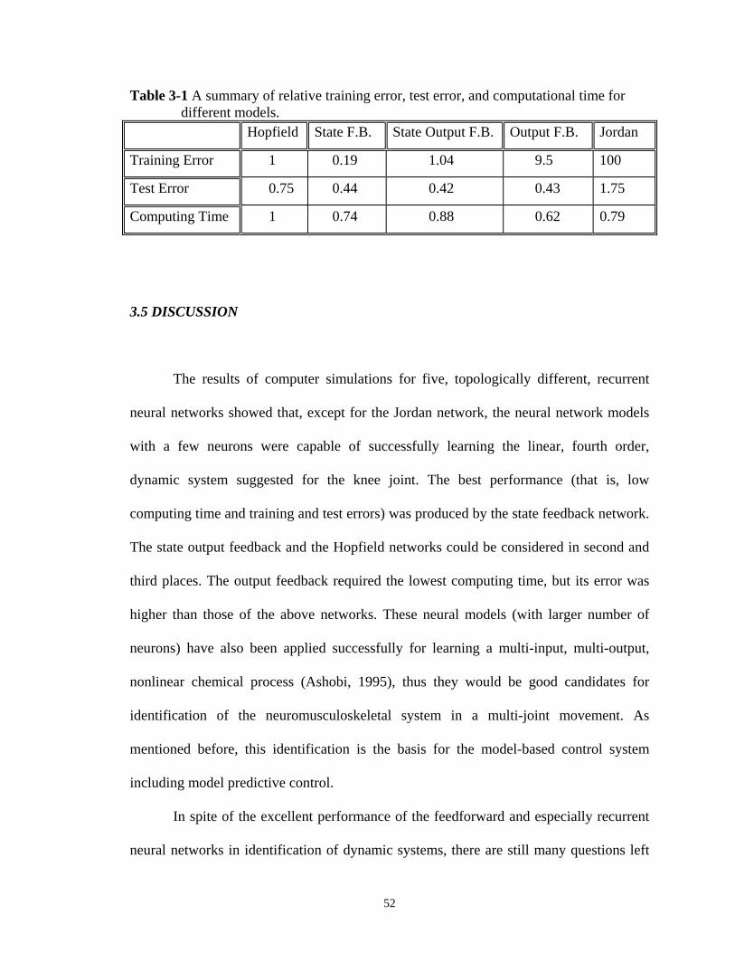
Table 3-1 A summary of relative training error, test error, and computational time for different models.

Hopfield State F.B. State Output F.B. Output F.B. Jordan

Training Error 1 0.19 1.04 9.5 100

Test Error 0.75 0.44 0.42 0.43 1.75

Computing Time 1 0.74 0.88 0.62 0.79

3.5 DISCUSSION

The results of computer simulations for five, topologically different, recurrent

neural networks showed that, except for the Jordan network, the neural network models

with a few neurons were capable of successfully learning the linear, fourth order,

dynamic system suggested for the knee joint. The best performance (that is, low

computing time and training and test errors) was produced by the state feedback network.

The state output feedback and the Hopfield networks could be considered in second and

third places. The output feedback required the lowest computing time, but its error was

higher than those of the above networks. These neural models (with larger number of

neurons) have also been applied successfully for learning a multi-input, multi-output,

nonlinear chemical process (Ashobi, 1995), thus they would be good candidates for

identification of the neuromusculoskeletal system in a multi-joint movement. As

mentioned before, this identification is the basis for the model-based control system

including model predictive control.

In spite of the excellent performance of the feedforward and especially recurrent

neural networks in identification of dynamic systems, there are still many questions left

52

unanswered. For example, how many neurons should the network have, what are the

suitable inputs for training the network, what is the proper sampling time, what is the

stability of the network. Unfortunately there is no formalized technique to answer these

questions currently, and they will remain for future investigation. The second question is

related to so-called "persisting excitation” in conventional system identification. Unlike

the traditional ARMA model, one of the limitations of neural networks is that there is no

relationship between the parameters of the network and the parameters of the physical

system being modeled. The information in the neural network model is distributed across

the parameters. This limitation prevents the use of a priori information to simplify the

model structure or the training process.

53

CHAPTER 4- MODEL PREDICTIVE IMPEDANCE CONTROL SCHEME

As discussed in Chapter 2, the model predictive impedance control is based on

using an impedance control strategy and a model predictive control algorithm. As the

widely studied version of impedance control, stiffness tuning strategy was suggested by

many researchers for increasing the resistance of joints against external disturbance as

well as for control of posture and movement. Hasan (1986) proposed a model for optimal

control of joint movements based on regulation of joint stiffness. His model considered

unperturbed (with no disturbance) movement and a load with no stiffness or viscosity.

For fast movements, the damping coefficient may not be ignorable. This model was thus

extended to include joint-load damping and passive stiffness and the external disturbance

(Towhidkhah et al., 1993). As a primary stage of general model evolution, the modified

model is discussed in the first section. Then, a comparison between MPC and the Smith

predictor model, suggested by Miall et al. (1993), is presented. Finally, the generalized

model is explained.

4.1 A SCHEME FOR JOINT MOVEMENT CONTROL USING STIFFNESS

REGULATION

The schematic diagram for control of joint movements based on stiffness

regulation is shown in Fig. 4-1. The trajectory selector receives information about the

duration of motion, the initial position, the final position, the dynamics of the joint-load

and spinal circuits, and the disturbance. Then it determines the optimal desired trajectory,

θd, and the proper active joint stiffness, σ. The desired trajectory is translated by the

54

feedforward controller into the proper slack angle trajectory, β. This controller is

basically the inverse dynamics of the spinal circuits and joint-load model. Having

received the information from the brain and sensory receptors, the spinal circuits and

muscles generate the required torque.

Trajectory

Selector

FeedforwardController

SpinalCircuits

andMuscles

Joint-LoadDynamics

Torque

DisturbanceReceptorsDelay

Brain ModelJoint Movement

Td

θσ

βθd

Fig. 4-1 The schematic diagram for adjusting the joint stiffness and slack angle. θd is desired joint angle trajectory; θ, actual joint angle trajectory; σ, active joint stiffness; β, slack angle trajectory; and Td, the external disturbance.

Optimizer

Program

Inverse Dynamic

Controller

DisturbanceGf(s)Delay

Td

θ

σ

βθdG(s)σDelay

βv

Fig. 4-2 The mathematical model of the stiffness control strategy. G(s) is the dynamics of joint-load; Gf(s), the transfer function of the feedforward pathway for external disturbance; and βv, the virtual equilibrium point.

55

Fig. 4-2 shows a mathematical model of the above scheme. G(s) is the dynamics

of the joint-load1; Gf(s) is a general block representing the dynamics of the feedforward

pathway for external disturbance; and βv is the virtual equilibrium point (see Fig. 2-4).

The time delays are due to spinal neurons and transmission pathways. The optimization

procedure and the criterion function are analogous to those applied by Hasan. He defined

the criterion function, a psychophysical sense of the subject’s effort, as:

(4.1) JT

= ∫ σ β.2

0

dt

where J is the criterion function, and β is the time derivative of the slack angle. For an

inertially loaded movement β.

can be described as:

.

β θσ

θ. .. ...

= + ( )I , (4.2)

and

JT

= +⎡⎣⎢

⎤⎦⎥∫ σ θ

σθ

.. ...( )I

0

2

dt

. (4.3)

I and θ are the inertia and angle of the joint, respectively.

1 The inertial-visco-stiffness load which is a linear function of joint angle is referred to as load and the other type of nonlinear load is referred to as an additive disturbance.

56

4.1.1 Computer Simulation and Results

In order to evaluate the performance of the model and the effect of the load and

disturbance on the control system, three cases were simulated on a microcomputer. In the

first and the second cases, the load and disturbance were added sequentially. The

dynamics of the receptor was assumed to be much faster than the dynamics of the closed

loop system and the variation of input signal, and the time delays were ignored. In the

third case, the above condition was removed. The criterion function can be written in

terms of the joint angle by using the dynamics of the neuromusculoskeletal system.

Assuming σ is constant as the first step, analytically minimizing the criterion function

equation then will yield the optimal θd (Hamiltonian method).

A model of the human knee joint found by Winters and Stark (1987) was used as

the model of the joint-load as follows:

G sIs Bs K

( ) =+ +

12 (4.4)

where I is the inertia of the knee (0.4 kgm2), B is the viscous damping of the knee

(3.2 Nms/rad), and K is the passive stiffness of the knee (6.4 Nm/rad). These parameter

values were obtained by Winters and Stark (1987) at 10% of maximal neural activity.

The feedforward controller was simulated using numerical differentiators.

Case 1- No Disturbance and No Time Delay:

A value for σ of 67 Nm/rad was found by trial and error to minimize the criterion

function. The initial position, final position, and duration of movement were set to 0, 0.4

rad, and 0.4 second, respectively. Fig. 4-3 shows the desired, actual, and slack angle

trajectories for this case.

57

Fig. 4-3 a) The slack angle (β), b) the desired position (θd) and actual

position (θ) for case 1 (σ=67 Nm/rad and Td=0). (From Towhidkhah et al., 1993).

Case 2- With Disturbance but with No Time Delay:

If the disturbance is not zero, the equilibrium position will not be specified by β

any more, but it will be determined by the virtual equilibrium, βv. Using Equation 2.1, Gf

is easily found to be equal to 1/σ if the dynamics of the feedforward pathway and the

delay time are ignored. It can be shown that by choosing Gf = 1/σ the “dynamic” effect

of the disturbance will be removed from the joint position. Thus the optimal desired

position found in Case 1 is still valid and can be applied in this case as well. The model

and parameter values used in the simulation were the same as before, and the disturbance

was changed from 0 to 30 Nm. The results of this simulation (Fig. 4-4) show that the

effect of disturbances have been completely removed from joint position.

58

Fig. 4-4 The effect of disturbance in case 2 (no receptor dynamics and no

delay pathways). a) Td=10 Nm. b) Td=30 Nm. (From Towhidkhah et al., 1993).

Case 3- With Disturbance and Time Delay:

In this experiment, Gf was assumed as a first order low pass filter with time

constant of 20 ms and the delay time of the feedforward and feedback pathways were

added to the model. The time delays were set at 10 ms. The desired and slack angle

trajectories that were used in this experiment were the same as those in the previous

cases. The results showed that increasing the amplitude of disturbance from 0 to +30 or -

30 Nm increases the error (see Fig. 4-5). It was also observed that increasing the joint

stiffness from 10 to 70 Nm/rad can reduce the error.

59

Fig. 4-5 The effect of change of

disturbance and stiffness on the error. The solid curve is θd, the dashed curve is θ and the dash-point curve is the error. σ=10, 25, 40, 55, 70 Nm/rad. The arrows show the direction of increasing of σ. a) Td=0 Nm. b) Td=-15 Nm. c) Td=15 Nm. d) Td=30 Nm. e) Td=-30 Nm. (From Towhidkhah et al., 1993).

4.1.2 Discussion

It was shown that the dynamic effect of the external disturbance can be removed

completely from joint position if the dynamics of receptors as well as the time delays of

pathways are ignored. For the high values of disturbance this assumption is unrealistic,

and the error is noticeable. The results showed that increasing the joint stiffness could

60

partially reduce the error, but, increasing joint stiffness too much could destabilize the

joint and cause oscillatory behavior. In the presence of load or disturbance, the subject’s

effort as the only factor in the criterion function is not sufficient. A function of output

error and disturbance should be added to find the optimal value of joint stiffness.

The above model is based on a feedforward inverse controller. Some of the

limitations of an inverse controller were discussed in Chapter 2. For linear physical

systems (causal systems) the inverse dynamics is noncausal and not physically realizable.

An approximation of the inverse dynamics is usually achieved in this case (such as the

above experiments). For non-minimum phase systems, the inverse dynamics results in an

unstable controller. For systems with time delays or non-one-to-one nonlinear systems

the inverse dynamics cannot be achieved.

One difficulty with a non-minimum phase system is that its initial response to a

step input is in the opposite direction of the steady state value; therefore, this system is

referred to as an “inverse response” system (Ogunnaike and Ray, 1994). This wrong

direction deceives an uninformed controller and causes a wrong command and usually

system instability. An inverse response may occur in a physical system which contains

opposing dynamic subsystems with different time constants (see Ogunnaike and Ray,

1994, for more details).

Time delays are also problematic factors in feedback control systems causing

system instability and leading to low gain and slow system response. A simple reason for

the system instability is that the system receives the wrong control signal either due to

comparing of the desired output (reference) with the “delayed” output (Fig. 4-6a) or due

to the “delayed” control signal (Fig. 4-6b). In contrast to closed loop systems, there is no

risk of instability due to time delay for open loop (feedforward) systems, and the

responses are only temporally shifted. The delay reported for proprioceptive feedback is

100-150 ms and for visual feedback about 200 ms (Hogan, 1985b, Miall et al. 1993).

61

PlantController

Delay

Control Signal OutputReference

(a)

PlantController Delay

Control SignalOutputReference

(b)

Fig. 4-6 Two systems with time delay. a) delay in feedback, b) delay in

feedforward.

Recently, Miall et al. (1993) suggested the Smith predictor as a likely model for

the cerebellum motor function. The Smith predictor was proposed in the 1950s (Smith,

1959) for control of engineering processes suffering from time delays. This technique

effectively shifts the time delay from inside the feedback loop to outside the feedback

and allows a higher loop gain and thus a faster response. A comparison of the Smith

predictor and MPC is presented in the next section.

62

Plant G(s)

Controller Gc(s)

Gm(s) - G*(s)

θβθd

Fig. 4-7 The Smith predictor control scheme. Gm(s) is the plant model, G*(s) is plant model with no time delay, θd is desired output, θ is actual output, and β is the control signal.

4.2 A COMPARISON BETWEEN MPC AND THE SMITH PREDICTOR

The Smith predictor control (SPC) scheme is shown in Fig. 4-7. G(s) represents

the plant transfer function and time delay; Gm(s), the plant model with time delay; G*(s),

the plant model with no time delay; θd, the desired output; θ, the actual output; and β,

control signal. A copy of the control signal is input to a block including the difference

between Gm(s) and G*(s), and the resulting output is subtracted from actual output and is

compared to the desired output.

Fig. 4-8 indicates a schematic block diagram for MPC. It is an adaptive control

system including two feedback mechanisms: a conventional feedback for correcting the

unpredicted disturbance, and an adaptation feedback through a model of the plant and

disturbance and an optimizer for minimizing the prediction error by tuning the gain of the

controller.

63

PlantController

Plant & Disturbance Model

Optimizer Td

θβ

θm

θd

Fig. 4-8 The model predictive control scheme. θd is desired output, θ is actual output, θm is the model output, Td is the external disturbance, and β is the control signal.

To compare the SPC and the MPC, a computer simulation experiment was carried

out. The experiment was divided into five different cases: perfect model, time delay

mismatch, filter mismatch, time delay and filter mismatch, and non-minimum phase. The

plant was the model of arm movement used by Miall et al. (1993). This model included a

first-order low-pass filter with a cut-off frequency of 0.9 Hz, an integrator, and a 150 ms

time delay. Table 4-1 summarizes the plant and the plant models applied in each case.

64

Table 4-1 A summary of the plant and the models applied in test of the Smith predictor and the model predictive control.

Plant Plant Model. Plant Time Delay Model Time Delay

Case I 1/[s(s+wc)] 1/[s(s+wc)] 150 ms 150 ms

Case II 1/[s(s+wc)] 1/[s(s+wc)] 150 ms 250 ms

Case III 1/[s(s+wc)] 1/[s(s+wm)] 150 ms 150 ms

Case IV 1/[s(s+wc)] 1/[s(s+wm)] 150 ms 250 ms

Case V (s-0.5)/[s(s+wc)] (s-0.5)/[s(s+wc)] 150 ms 150 ms

wc = 2*π*(0.9), wm = 2*π*(0.54), and Gc=20.

The results of computer simulation are shown in Fig. 4-9 and are summarized in

Table 4-2. For the perfect model, Case I, Fig. 4-9a shows that the SPC response follows

the reference with a delay (as expected), but the MPC response achieves the reference

after a short period of time. For the model mismatch cases, Cases II-IV, both control

systems produce higher errors compared with the first case; the MPC errors, however, are

less than those of the SPC (see also Table 4-2). For the non-minimum phase case, Case

V, the MPC error is very low, and the SPC error is high and is increasing due to the

instability resulting from numerical error of model realization.

Table 4-2 A summary of the SPC and MPC root mean square errors.

Case I Case II Case III Case IV Case V

SPC Error 0.2664 0.3096 0.3271 0.3830 0.2485

MPC Error 0.0519 0.1363 0.1428 0.2525 0.0303

65

-1.2

-0.6

0

0.6

1.2

0 1 2 3 4 5 6 7Time (s)

Am

plitu

de

Ref. S. P. MPC

-0.4

0

0.4

0 1 2 3 4 5 6 7Time (s)

Err

or

S.P. MPC

Fig. 4-9a Comparison between the Smith predictor and model predictive control outputs for perfect models.

66

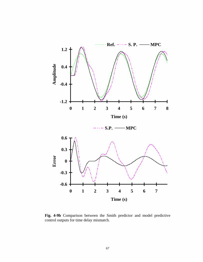
-1.2

-0.4

0.4

1.2

0 1 2 3 4 5 6 7 8

Time (s)

Am

plitu

de

Ref. S. P. MPC

-0.6

-0.3

0

0.3

0.6

0 1 2 3 4 5 6 7

Time (s)

Err

or

S.P. MPC

Fig. 4-9b Comparison between the Smith predictor and model predictive control outputs for time delay mismatch.

67

-1.2

-0.8

-0.4

0

0.4

0.8

1.2

0 1 2 3 4 5 6 7

Am

plitu

deRef. S. P. MPC

-0.5

-0.25

0

0.25

0.5

0 1 2 3 4 5 6 7

Erro

r

S.P. MPC

Fig. 4-9c Comparison between the Smith predictor and model predictive control outputs for filter mismatch.

68

-1.5

-0.5

0.5

1.5

0 1 2 3 4 5 6 7

Am

plitu

deRef. S. P. MPC

-0.8

-0.4

0

0.4

0.8

0 1 2 3 4 5 6 7

Erro

r

S.P. MPC

Fig. 4-9d Comparison between the Smith predictor and model predictive control outputs for filter mismatch.

69

-1.4

-0.7

0

0.7

1.4

0 1 2 3 4 5 6 7

Am

plitu

deRef. S. P. MPC

-0.4

0

0.4

0.8

0 1 2 3 4 5 6 7

Erro

r

S.P. MPC

Fig. 4-9e Comparison between the Smith Predictor and model predictive control outputs for filter mismatch.

70

- Discussion

Computer simulations for all cases showed a better performance of the model

predictive control to the Smith predictor suggested by Miall et al. For a perfect model of

the non-minimum phase plant, the SPC showed an unstable response. An increase in the

instability is expected for a non-perfect model.

One reason for higher errors of the SPC is that its gain is fixed, in contrast to the

MPC which enjoys an adaptive gain. Indeed, the focus of Miall et al.’s paper is on the

cerebellum motor function and the model of the plant. No attention was given to the

controller and other motor centers, such as the motor cortex, involved directly in the

control of movement. This issue is considered in the MPC.

Another advantage of the MPC is that it uses a temporal (step/impulse) response

model rather than a transfer function model. This makes the MPC attractive for nonlinear

and multi-input multi-output systems which are difficult to model in terms of transfer

functions. Moreover, the optimization basis of MPC allows the controller to explicitly

deal with the operating constraints.

4.3 MODEL PREDICTIVE IMPEDANCE CONTROL SCHEME

Based on the principles mentioned in Chapter 2 and in Fig. 2-6, the model

predictive impedance control scheme is shown in Fig. 4-10. There are two levels of

control: the spinal level and the cortical level. Both levels receive information about joint

position and velocity (θ and θ.

respectively) and the environment (disturbance). The

spinal loop compensates for small perturbations, and the long loop through the brain

corrects large perturbations by adjusting the muscle/joint impedance. The desired

position trajectory and velocity profile, θd and θ are defined by the trajectory selector. .

d

71

β and β are determined by the feedforward controller which acts based on the model

predictive control (MPC) algorithm discussed in Chapter 2. The position and the velocity

errors are multiplied by joint active impedance σ and b respectively. G1(s) and G2(s) are

dynamics relating to the generation of the myoelectric signal and of the muscle forces

which can be assumed as first order systems (Winters and Stark, 1987). Passive

mechanical joint impedance due to connective tissue, bones, and load are modeled as

joint-load dynamics G3(s). The internal loop that includes G1, G2, and G3 is the model of

the musculoskeletal system, which will be referred to as the system hereafter. The net

torque due to other joints and sources is added to the muscles' torque as the external

disturbance input. This increases the capability of the model to study a single joint

movement in more complex multi-joint motion. The sensory information about actual

joint movement (θ and θ ) and the disturbance as well as a copy of the control variables

are received by an identifier in the brain model which provides models of the

musculoskeletal system, the disturbance dynamics, and processing and transmission time

delays. These models are used by the feedforward controller to find optimal control

signals (β and β ).

.

.

.

72

Feedforward Controller

Identifier

Brain Model

Delay

β

b

β.

M P C and

Algorithm Adaptation

σ

EMG

Torque

Joint-Load

+ +

+ +--

Selector Trajectory

+

.θθ

+

System-Disturbance

Models

Receptors

dθ.dθ

Delay

Receptors

Td

G3(S)

G2(S)

G1(S)

Fig. 4-10 The model predictive impedance control scheme. θd and θ.

d are desired joint angle and angular velocity. θ and θ

. are actual joint angle and

angular velocity. θm is measured joint angle. Td is the external disturbance. G1(s) and G2(s) are dynamics relating to the generation of EMG signal and muscles’ torque; and G3(s) is joint-load dynamics.

73

In fact, the model includes two controllers. The active joint impedance has the

effect of being a low level PD (proportional and derivative) controller in the internal loop

doing fast and minor compensation and short term prediction. The model predictive

controller is the high level controller doing the major compensation and long term

prediction.

A possible biological interpretation for the trajectory selector, the feedforward

controller, and the identifier could be the association cortex, the motor cortex, and the

cerebellum respectively. Based on previous experience and sensory information, the

associative cortex and the lateral part of the cerebellum select the desired trajectory and

send it to the motor cortex which acts as an executive motor center and provides motor

commands dictating the required impedance and equilibrium points through α and γ

motoneurons. The intermediate and the lateral parts of the cerebellum have been

suggested as the most important motor centers involved in short term and long term

predictions (Ito, 1984; Stein, 1986). The cerebellum is theorized to receive afferent

information from the results of movements as well as an efferent copy of motor

commands. This information allows the cerebellum to create a system/disturbance model

and to update it (see Miall et al., 1993 for review).

-Disturbance Model

The external disturbance may be categorized into two groups from an input point

of view: a measurable disturbance and an unmeasurable disturbance. The first group can

be measured directly or indirectly through receptors and can be modeled the same way

74

which the plant is modeled. In lifting a load, for example, the load torque may be

measurable through the Golgi tendon organs and pressure receptors. This group also

includes the known but uncontrolled sources which affect the movement such as body

weight or ground reaction during walking.

The second group may in turn be divided into two types from the output point of

view: predictable and unpredictable. An unmeasurable-predictable disturbance may be

modeled indirectly through its effect on the output response. A typical method is to

assume a random white noise as a disturbance input added to the system through a black

box disturbance model. This model represents the history of the disturbance being

extracted from output measurements (for more detailed techniques see Ljung, 1987;

Ljung and Soderstrom, 1983). Periodic disturbance may be considered as this type of

disturbance. There is no model for the unmeasurable-unpredictable disturbance, and the

errors resulting from this type of disturbance must be corrected through a feedback

mechanism. The mismatch between the musculoskeletal system and its model internal to

the MPC is an example of this category.

The disturbance Td in Fig. 4-10 represents the total disturbance of which the

measurable portion is measured by the receptors. The identifier embodies a model of the

measurable disturbance and an estimation (model) of any unmeasurable disturbance.

In learning a new movement, the control system is switched gradually from

closed loop mode to open loop mode. In the primary stage of learning, when the model of

the system and the external disturbance is poor, the error correction is carried out by the

cortical feedback and internal loops. The joint impedance is set at a high value to increase

the joint resistance against unknown external disturbances and the system dynamics. In a

75

multi-joint movement, increasing the stiffness of joints is also helpful to decrease the

degree of freedom (joints’ flexibility) which makes the control task simpler. The model is

improved by more practice. This reduces the prediction error and allows applying lower

impedance and increasing the joint’s flexibility. At the end of the learning process, when

the model is accurate enough, the cortical feedback may be removed (feedforward mode).

An example is helpful to clarify the above process. Consider a driver who is

driving a car on a road for the first time. The road is unknown to him and high attention

is required. The road signs help the driver to predict and be prepared for curves and

dangerous areas (short term prediction). After several times over the road, the driver

becomes familiar with the road and learns a perspective about it and its dangerous areas

(long term prediction). In this case he needs less attention than before. He may also be

able to drive simply on the road with no signs. The road traffic could be assumed as a

disturbance- unpredictable usually.

4.4 DISCUSSION

The equilibrium point hypothesis (EPH) is an essential theory in motor control.

The key point in the equilibrium point hypothesis is that the movement trajectory may

result from a natural interaction between the musculoskeletal system dynamics, the

external load, and spinal reflexes, rather than a complicated control mechanism such as

the inverse dynamic approach. It is the author’s belief that although the dynamics of the

musculoskeletal system and the environment play a significant role in the generation of

76

some movements, the role of the motor centers in the brain generally has been

oversimplified or has not been sufficiently discussed in the current equilibrium point

models. For example, the unstable (inverted pendulum) characteristic of the standing leg

and the oscillatory behavior of the swinging leg and arms in normal walking are

important factors in generation of the walking rhythms, but this is not extendible to the

movements or skills which need a great mental effort. Furthermore, the evidence for the

EPH is mainly based on simple positioning movements, but for dealing with more

complex movements, the equilibrium point models should be modified with more

emphasis on the higher control levels. The model predictive controller proposed in this

thesis is a possible modification for EP models and a bridge for the gap mentioned above.

The controller also presents a method to use a priori knowledge of the

neuromusculoskeletal system and environment to adjust the equilibrium point.

One problem with model-based control systems (for example, the Smith

predictor) is that model mismatching (inaccuracy) may worsen system behavior rather

than improve it. To solve this problem two methods can be followed: an adaptive

mechanism which updates the model at time intervals and a nonadaptive robust controller

which is not sensitive to system uncertainties and system parameter variation. The

method employed in MPIC is based on the combination of these two methods; that is, on

the one hand the identifier updates the system/disturbance model, and on the other hand,

any model mismatching can be compensated by the robust optimal controller and joint

impedance adjustment.

An MPIC model is consistent with the servo control model suggested by

McIntyre and Bizzi (1993). They concluded that for fast movements, adding a viscosity

77

input to the position servo control model decreases the required stiffness values to the

range observed experimentally.

A natural realization of the identifier and the controller is a neural network. It was

indicated in Chapter 3 that artificial neural networks were capable of learning the

dynamics of the system and the external dynamics. Thus, it is similarly possible that the

biological neural networks also use information about the dynamics of movements and

environment and apply this knowledge in adjusting the control variables (joint

impedances for example).

As with any optimization-based technique, the MPC algorithm needs extensive

computational effort to find control signals, particularly for multi-joint movements. This

limitation may be obviated by use of neural networks. With some modification, the

cascade neural network in the Hirayama et al. (1993) model may be one possible neural

realization for the model predictive controller. The network includes neural units

connected to each other in cascade. Each unit represents a one-step-ahead predictor. In

the context of MPC, the prediction horizon determines the total number of neural units,

and the control horizon determines the numbers of the neural units which generate the

output torques.

It is reasonable to assume that the CNS applies different horizons and

performance indexes in different learning stages. Unfortunately, there is no analytical

technique currently available for finding the best values of the horizons, so the

relationship between the proper horizons and learning stages or different movements

remains for further research. However, a longer prediction horizon allows the controller

to apply more system information thereby producing more efficient control signals.

78

Ideally, if the model is perfect and there is no unpredicted disturbance, the control signals

can be computed once for the entire trajectory. No feedback nor extra computation for

control signals are required in this case. It seems that in the early stage of learning, when

the model is poor, the model error is high, thus, choosing shorter horizons may reduce the

prediction error. The feedback mechanism is essential at this stage for error correction

and high impedance increases the system tolerance to the external disturbance or model

error. At the final stage of learning, when the model is sufficiently accurate, the

prediction error is low and longer horizons can be chosen. The feedback mechanism is

less important and joint impedance may decrease to allow more flexibility and fine

control.

4.5 SUMMARY

Model predictive impedance control is a unification of the equilibrium point

hypothesis (both α and λ models), the impedance control strategy, servomechanism

theory, and optimization-based model predictive control. It is the first time that model

predictive control has been applied in modeling the human motor control system. This

controller suggests a possible bridge between the EPH and the neural motor centers in the

brain and provides a practical technique to adjust the equilibrium point and the joint

impedance using the information of the neuromusculoskeletal system and the

environment. MPIC is an adaptive model with learning ability. It can operate in open-

loop or closed-loop manners. The optimization basis of the model increases its flexibility

by tuning the cost function and weighting factors for different tasks.

79

CHAPTER 5- APPLICATION OF THE MODEL PREDICTIVE IMPEDANCE CONTROL SCHEME

Model predictive impedance control was discussed in Chapter 4. This chapter

deals with the application of MPIC to the study of three quite different movements

including a regular rhythmic movement, a tracking movement in the presence of an

unknown disturbance, and a biped model of human walking. The objectives of this study

were first to compare the model output for the optimal values of the joint impedance with

the experimental observations and second to investigate the control model sensitivity

(that is, robustness) to model mismatching.

For simplicity, β was assumed as the derivative of β and the dynamics of the

receptors were ignored. The computer programs were written in the MATLAB language

(MathWorks Inc., 1992), and quadratic programming was employed by the MPC

algorithm (Morari and Ricker, 1994) for the first stage of optimization with the

performance index introduced in Equation 4.3. For the rhythmic and the tracking

movements the horizon factors were set to M=3 and P=20 based on experience for

engineering systems (Morari et al., 1992; Ashobi, 1995), and weighting factors were

changed from 0 to 10 and finally were set to qk=10, and rk=5 to generate relatively lower

error and smoother control signals. The second stage of optimization was based on a grid

search in which the joint stiffness and viscosity were changed from 1 to 200 Nm/rad by

step size of 10 Nm/rad and 0 to 50 Nms/rad by step size of 5 Nms/rad, respectively. For

.

81

each impedance value, the total root square error between the model response and the

desired response was obtained from the experimental data. The minimum error specified

the optimal value of the joint impedance.

5.1 RHYTHMIC MOVEMENT

In the study of rhythmic movement (Towhidkhah et al., 1994c), the knee angle

trajectory and the external torque disturbance were taken from Winter's data during

human walking (Winter, 1991). The external disturbance in this case represents the net

torque resulting from weight loading, ground reaction, and the forces acting on the other

joints. The movement was assumed to be well learned, that is, models of the

neuromusculoskeletal system and the disturbance were introduced to the controller with

no mismatch. The musculoskeletal model of a joint comprising three blocks, G1, G2, and

G3, were defined using Winters and Stark (1987) results as follows. The dynamics

related to generating the neural drive was

G (s) 1T s 11

1=

+ (5.1)

where T1=85 ms. The dynamics of generating the muscles’ torque was

G (s) 1T s 12

2=

+ (5.2)

where T2=35 ms. The passive joint-load dynamics was represented by

G (s) 1Js Bs K

3 2=+ +

. (5.3)

82

The values used for passive impedance were J = 0.4 kgm2, B = 5.2 Nms/rad, and K = 17

Nm/rad. These parameter values were the average of those found by Winters and Stark

(1987) for the human knee joint at 10% and 50% of maximal neural activity. The

feedback time delay was ignored in this simulation because the movement was close to

an open loop movement. Fig. 5-1 shows the error function with respect to joint stiffness

and viscosity. The optimal values for σ and b were found to be 1 Nms/rad and 5 Nm/rad

respectively showing the relative importance of the viscosity factor with respect to the

stiffness factor. The high error values at the corners of the error function are due to

system instability resulting from high stiffness which can be reduced by proper tuning of

viscosity as seen. Fig. 5-2a shows a comparison of the experimental (desired) and the

model response trajectories for optimal values of joint impedance. Although the model

response follows the experimental trajectory well for the swinging period (area I), the

error is relatively high for the standing period (area II). A better result was achieved by

increasing the horizon factors to M = 20 and P = 50 (see Fig. 5-2b).

83

Fig. 5-1 Error function with respect to joint stiffness (Nm/rad) and viscosity (Nms/rad) for the rhythmic movement.

84

0 0.5 1 1.5 2 2.5 3-0.2

0

0.2

0.4

0.6

0.8

1

1.2

Join

t Ang

le (r

ad)

Time (s)Standing PhaseSwinging Phase

( I ) ( II )

(a)

0 0.5 1 1.5 2 2.5 30

0.2

0.4

0.6

0.8

1

1.2

Join

t Ang

le (r

ad)

Time (s)Standing PhaseSwinging Phase

( I ) ( II )

(b)

Fig. 5-2 Desired joint angle trajectory (solid curve) and model’s output trajectory (dotted curve) for optimal values of joint impedance for the rhythmic movement. I shows the swing phase and II shows the standing phase. a) for M=3 and P=20. b) for M=20 and P=50.

5.2 TRACKING MOVEMENT

In the study of tracking movement (Towhidkhah et al., 1994b), a sigmoidal

trajectory was selected as a desired knee angle trajectory, and an unpredicted 10 Nm step

85

disturbance was added to the model after 1.1 seconds. The dynamics of G1, G2, and G3

were the same as in the rhythmic movement, and the feedback time delay was assumed to

be 100 ms. In contrast to the rhythmic movement, in this case the controller had no pre-

information about the disturbance dynamics. The error function and the output

trajectories for this case are indicated in Figs. 5-3 and 5-4 respectively. The optimal

impedance values were σ = 60 Nm/rad and b = 35 Nms/rad showing a relatively higher

importance required for the unpredicted external disturbance. The system instability

referred to in the results shown in Fig. 5-1 is seen more clearly in Fig. 5-3. In Fig. 5-4a,

stiffness control (viscosity set to zero) is compared with impedance control (Fig. 5-4b).

As expected, high stiffness required for load compensation results in oscillatory behavior

(see Fig 5-4a). This behavior is improved by using a proper value of viscosity.

When the model of the disturbance dynamics was introduced to the controller, the

error function was very close to the case in which there was no disturbance. In other

words, once the model of the system and the disturbance are known perfectly by the

identifier, the effect of the disturbance can be removed precisely. Results for this

simulation are not presented as there was no observable difference between the actual

and desired trajectories.

86

Fig. 5-3 Error function with respect to joint stiffness (Nm/rad) and viscosity (Nms/rad) for the tracking movement.

87

Fig. 5-4 A comparison of the desired trajectory (solid curve) and output trajectory (dotted curve). a) for nonoptimal values of joint impedance, σ = 70 Nm/rad, and b = 0. Total root square error is 1.18 rad. b) for optimal values of joint impedance, σ = 60 Nm/rad, and b = 35 Nms/rad. Total root square error is 0.2 rad.

88

5.3 BIPED MODEL FOR WALKING

In the third study a more complex system model was selected. It was a simplified

kneeless biped model (Towhidkhah et al., 1995) shown in Fig. 5-5. The regular

pendulum represents the swinging leg, and the inverted pendulum represents the standing

leg. The standing leg angle is to be controlled by the muscles' torque. The dynamic

equations may be found by the Lagrangian method (see Wells, 1967) as follows:

( ) ( ) ( ) ( ) ( )

( ) ( ) ( )

.. ..

.. ..m m l m l l Cos m l l Sin gl m m Sin T

m l m l l Cos m l l Sin gm l Sin

+ − − − − − − − + =

− + − − + − − − − =

12

1 1 1 1 1

1 1 1 1 1 1 1 1 0

θ γ π γ θ γ π γ θ θ

γ θ π γ θ θ π γ θ π γ

(5.4)

where m is the mass of the body and trunk, m1 is the mass of the swinging leg, l is the

length of standing leg, l1 is the distance between the hip joint and the swinging leg mass

center, θ is the angle of the ankle joint, γ is the angle of the swinging leg, T is the

muscles’ torque for the ankle joint, and g is gravitational acceleration. The muscles’

torque for the hip joint and the mass of the standing leg have been ignored for simplicity.

G3 is determined by linearization of the equations for small angle deviations:

(5.5) ( ) ( )

.. ..

.. ..m m l m l l gl m m T

m l m l l gm l

+ − − + =

− − − =

12

1 1 1

1 1 1 1 1 1 0

θ γ θ

γ θ γ

For m=50 kg, m1=10 kg, and l=1 m, G3 is :

G (s) s 9.8s 104.77

32

4=+

−. (5.6)

89

θ mg

mlγ

HAT

Swinging Leg

Standing Leg

Fig. 5-5 The biped model for human walking. γ is the angle of the swinging leg, θ is the angle of standing leg, m is the mass of body and m1 is the mass of the swinging leg. HAT represents head, arms, and trunk.

At the end of each cycle, the swinging leg becomes the standing leg for the next cycle

and vice versa. To model this, the final conditions of the swinging leg (γ and γ ) from one

cycle were used as the initial conditions for the standing leg (θ and θ ) of the subsequent

cycle. Thus, in contrast to the two previous cases, the system dynamics in this case was

time varying and unstable. The desired trajectory for the ankle joint was calculated from

Winter's experimental results for a footless ankle joint (Winter, 1991).

..

90

X =AX+BUY =CX+DU

.

bS + σ

M P C

x0

1 2

_____________(T1S+1)(T2S+1)

1

Step Function

Pendulum Dynamics

Dynamic Impedance PD Controller)

Angle of Ankle Joint

Identification Control

Desired Trajectory

Fig. 5-6 The simulation procedure for the study of biped model. X0 is the initial condition. The switch condition 1 is for identification of the system and the switch condition 2 is for control of the system.

The simulation procedure contained two phases: identification phase and control

phase (see Fig. 5-6). The joint stiffness and viscosity were set to fixed values in each

simulation. The dynamics of the biped model was presented in the form of state space to

allow changes in initial conditions, X0. In the identification phase, phase 1, the step

91

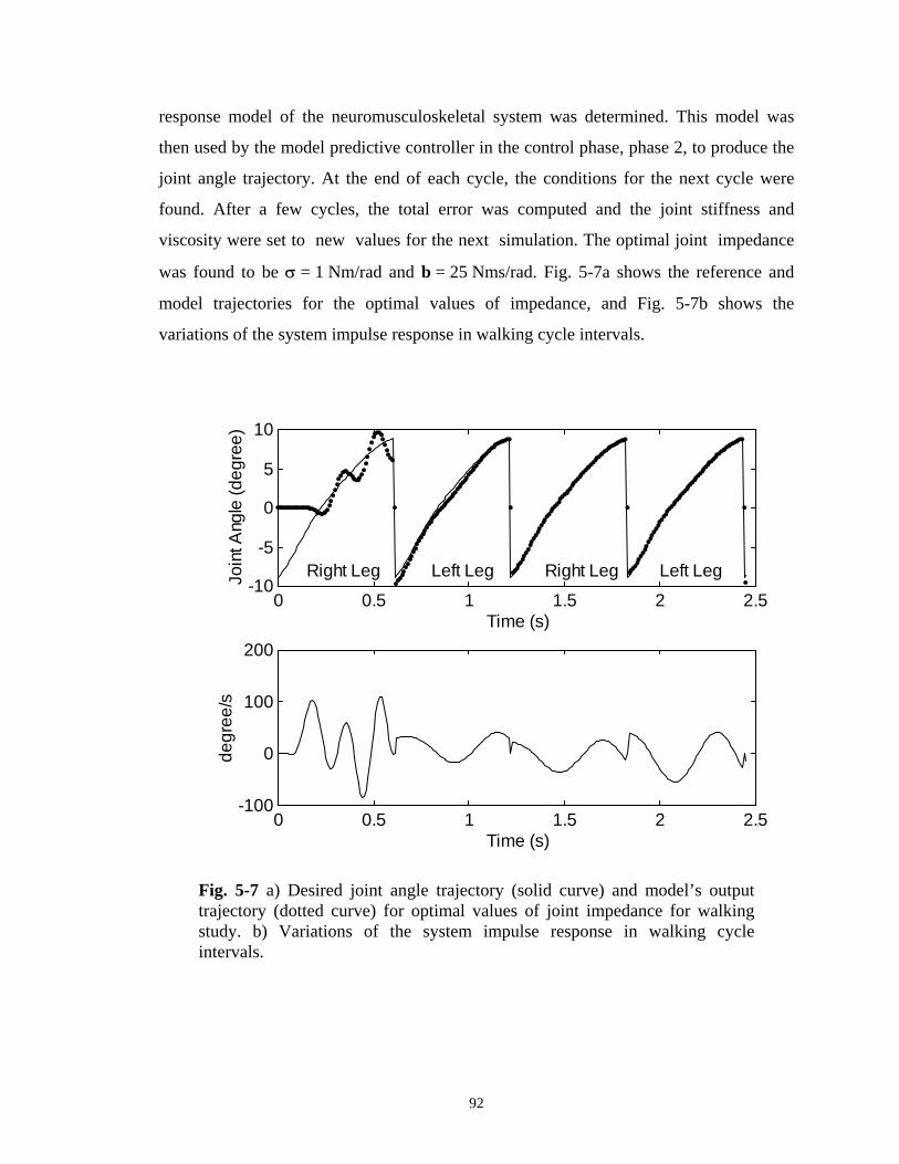
response model of the neuromusculoskeletal system was determined. This model was

then used by the model predictive controller in the control phase, phase 2, to produce the

joint angle trajectory. At the end of each cycle, the conditions for the next cycle were

found. After a few cycles, the total error was computed and the joint stiffness and

viscosity were set to new values for the next simulation. The optimal joint impedance

was found to be σ = 1 Nm/rad and b = 25 Nms/rad. Fig. 5-7a shows the reference and

model trajectories for the optimal values of impedance, and Fig. 5-7b shows the

variations of the system impulse response in walking cycle intervals.

0 0.5 1 1.5 2 2.5-10

-5

0

5

10

Time (s)

Join

t Ang

le (d

egre

e)

Right Leg Left Leg Right Leg Left Leg

0 0.5 1 1.5 2 2.5-100

0

100

200

Time (s)

degr

ee/s

Fig. 5-7 a) Desired joint angle trajectory (solid curve) and model’s output trajectory (dotted curve) for optimal values of joint impedance for walking study. b) Variations of the system impulse response in walking cycle intervals.

92

5.4 SYSTEM AND MODEL MISMATCH

No model is perfect and no two individuals have identical dynamics

characteristics. Thus, the evaluation of the control system robustness is necessary, and

the sensitivity to model mismatch should be tested. The tests were divided into three

categories: system parameters mismatch, external disturbance mismatch, and applying a

neural network model as the system identifier.

5.4.1 System Parameters Mismatch

In this experiment, three levels of mismatching, that is, 15%, 30%, and 45% were

defined for each passive impedance parameter (J, B, K, and T2), their combination (J-B-

K), and the loop gain (g) in the rhythmic and tracking movements. For the tracking

movement, the effect of time delay mismatch (td) was also investigated. The horizon

factors were set to be M = 3 and P = 20 for all cases. For more efficient comparison, the

values of the joint impedance for the mismatch cases and non-mismatch case were set to

the same values. The total root square error results are shown in Tables 5-1 and 5-2.

Table 5-1 The root square errors (rad) for parameter mismatch in the rhythmic movement study.

0% Mismatch 15% Mismatch 30% Mismatch 45% Mismatch J 1.43 1.61 2.30 3.27 B 1.43 1.94 2.51 3.04 K 1.43 1.48 1.59 1.73 T 1.43 2.32 2.50 2.75 g 1.43 1.61 2.28 3.02 J-B-K 1.43 1.53 3.14 6.59 J, B, K, T represent individual passive impedance mismatch, g represents gain mismatch, and J-B-K represents a combined mismatch. σ=1 Nm/rad, b=5 Nms/rad, M=3, and P=20.

93

Table 5-2 The root square errors (rad) for parameter mismatch in the tracking movement study.

0% Mismatch 15% Mismatch 30% Mismatch 45% Mismatch J 0.41 0.42 0.44 0.46 B 0.41 0.43 0.45 0.47 K 0.41 0.43 0.46 0.48 T 0.41 0.42 0.43 0.44 g 0.41 0.40 0.48 0.86 td 0.41 0.45 0.50 0.57 J-B-K 0.41 0.44 0.51 0.70 J, B, K, T represent individual passive impedance mismatch, g represents gain mismatch, td, time delay mismatch, and J-B-K, a combined mismatch. σ = 60 Nm/rad, b = 15 Nms/rad, M = 3 and P = 20.

Better error results were found when the joint impedance in each case was adjusted to the

optimal values corresponding to that case (see Table 5-3 for the tracking movement).

Table 5-3 The optimal root square errors (rad) for parameter mismatch in the tracking movement study.

0% Mismatch 15% Mismatch 30% Mismatch 45% Mismatch J 0.2010 0.2354 0.2612 0.2762 B 0.2010 0.2154 0.2379 0.2569 K 0.2010 0.2263 0.2445 0.2700 T 0.2010 0.2300 0.2608 0.2804 g 0.2010 0.2814 0.3709 0.4764 td 0.2010 0.1606* 0.1575* 0.2112 J-B-K 0.2010 0.2915 0.3739 0.4456 J, B, K, T represent individual passive impedance mismatch, g represents gain mismatch, td, time delay mismatch, and J-B-K, a combined mismatch. M = 3 and P = 20.

In addition to tuning the joint impedance in each mismatch case, further improvement

may be attainable by varying the control and prediction horizons (see Figs. 5-11 and 5-

13).

94

5.4.2 External Disturbance Mismatch

For disturbance model mismatch, in rhythmic movement, the approximate

disturbance models (see Fig. 5-8a) were generated by the variance of Winter's data

(Winter, 1991). The disturbance models include Dist, Dist-p, and Dist-n. Dist-p

represents a positive disturbance compared to Dist, and Dist-n represents a negative

disturbance compared to Dist. The model Dist was introduced to the controller as the

model of the disturbance for all three cases. The horizons were set to M = 20 and P = 50

for a better result. Fig. 5.8b indicates acceptable output trajectories for these three cases.

Fig. 5-8 (a) Different disturbances applied to the model. Dist (solid curve) is the disturbance model used, Dist-p (dashed curve) is the disturbance applied to the system with positive mismatch, and Dist-n (dotted curve) is the disturbance applied to the system with negative mismatch. (b) The results of disturbance mismatch test. Output (solid curve), Output-p (dashed curve), and Output-n (dotted curve) are outputs regarding to the application of Dist, Dist-p, and Dist-n to the system respectively.

* The errors for 15% and 30% mismatch are less than that of 0%. The reason is that the impedance values applied in computer simulation were quantized values. The errors, therefore, are quasi-optimal.

95

5.4.3 Applying Neural Network Model

In Chapter 3, it was shown that dynamic recurrent neural networks with different

topologies were able to learn the dynamics of the neuromusculoskeletal system and the

external disturbance. In the next experiment, a recurrent neural network model with state

feedback (see Fig. 3-5) was applied as the identifier in the control system scheme. The

network was trained based on the procedure mentioned in Chapter 3. Fig. 5-9 shows a

comparison between the step responses resulting from the mathematical and the neural

models. These responses applied to the controller in the tracking movement and the

results are shown in Fig. 5-10. The total root square errors for the mathematical model

and the neural model are 0.3069 rad and 0.3221 rad, respectively.

96

0.00

0.10

0.20

0.30

0.40

0.00 0.30 0.60 0.90

Time (s)

Rad

.

System NN

Fig. 5-9 Step responses of the neuromusculoskeletal system and its neural network model.

0.00

0.25

0.50

0.75

1.00

0.00 0.60 1.20 1.80 2.40 3.00

Time (s)

Rad

.

Ref. Math. NN

Fig. 5-10 The results of application of neural network model in control of the neuromusculoskeletal system for the tracking movement.

97

5.5 EFFECTS OF CHANGING THE HORIZON FACTORS

In addition to the neuromusculoskeletal system and the external disturbance

dynamics, the error function and the optimal values of joint impedance depend on the

control and prediction horizons as well as the degree of the models’ mismatch (degree of

training for example). It is possible that for different degrees of mismatch, the predictive

controller selects different values for the horizons and joint impedance. What the best

values are for the horizons for an specific movement or environment, and how they may

change during a learning process remain for further research. However, preliminary

results showed that, for the rhythmic movement (a well learned movement), longer

horizons were preferable, and for the tracking movement with an unexpected disturbance,

shorter horizons were preferable due to high prediction error. Moreover, for a rhythmic

movement, the time period of a cycle would be a good candidate for the prediction

horizon. The computer simulation carried out is as follows.

Both the rhythmic and the tracking movements were studied in this experiment.

The J-B-K case with four degrees of mismatch, that is, 0%, 15%, 30%, and 45% were

selected. Eight combinations for the horizons were applied: 1) M = 3 and P = 10,

2) M = 3 and P = 20, 3) M = 3 and P = 30, 4) M = 3 and P = 40, 5) M = 3 and P = 50,

6) M = 10 and P = 25, 7) M = 10 and P = 50, and 8) M = 25 and P = 50. For each case

the minimum error and the optimal values of joint impedance were determined.

The minimum errors and the corresponding optimal values of impedances for

each case are shown in Figs. 5-11 and 5-12 for the rhythmic movement and in Figs. 5-13

and 5.14 for the tracking movement. Figs. 5-11 and 5-13 show that, first, the average

98

error increases by increasing the degree of mismatch. For rhythmic movement, the errors

for 0% mismatch and 15% mismatch are very close. Second, the results show that the

change of horizons for 0%, 15%, and 30% mismatch has no important effect on errors.

Third, the cases with close relative horizons (M/P), that is, cases 1, 6, 7, and 8, produce

close error values. This suggests that in addition to the horizons’ absolute values, their

relative values may be an important factor in control of movements. Figs. 5-12 and 5-14

show the changes in the optimal values of the joint impedances when horizons and

degree of mismatch change. As seen, when the degree of mismatch increases, the optimal

values tend toward lower values, and the scatter of the optimal values decreases. When

the degree of mismatch is high, low values of impedance decrease the gain and sensitivity

of the neuromusculoskeletal system resulting in a lower error.

99

Fig. 5-11 The results of changes in minimum errors due to changes in horizons and degree of mismatch for the rhythmic movement. For horizontal axis: 1 means M=3 and P=10, 2, M=3 and P=20, 3, M=3 and P=30, 4, M=3 and P=40, 5, M=3 and P=50, 6, M=10 and P=25, 7, M=10 and P=50, and 8, M=25 and P=50.

100

Fig. 5-12 The variations of the optimal points with respect to horizons and degree of mismatch for the rhythmic movement.

101

Fig. 5-13 The results of changes in minimum errors due to changes in horizons and degree of mismatch for the tracking movement. For horizontal axis: 1 means M=3 and P=10, 2, M=3 and P=20, 3, M=3 and P=30, 4, M=3 and P=40, 5, M=3 and P=50, 6, M=10 and P=25, 7, M=10 and P=50, and 8, M=25 and P=50.

102

Fig. 5-14 The variations of the optimal points with respect to horizons and degree of mismatch for the tracking movement.

5.6 DISCUSSION

The simulation results show an acceptable performance of the model predictive

impedance control scheme in different types of movements. The model responses for the

103

optimal impedance values are close to the natural human responses and in agreement

with reported investigations.

The results of the biped model study indicate that the control model is able to

control the unstable and oscillatory biped system. This is due to two factors: the MPC

algorithm and joint impedance tuning. In fact, the model includes two controllers. The

active joint impedance has the effect of being a low level PD (proportional and

derivative) controller in the internal loop doing fast and minor compensation and short

term prediction. This controller is very helpful in stabilizing the biped dynamics, that is,

keeping balance in posture mode. The model predictive controller is the high level

controller doing the major compensation and long term prediction.

For a tracking movement with an unpredictable disturbance, higher impedance is

preferable. For example, in the early stages of learning a new skill when the external

disturbance model is poor, increasing joint impedance may be used by the CNS to

increase the tolerance of the system to external disturbance (Grillner, 1972; and Houk,

1979). This also decreases the degrees of freedom, in a multi-joint movement, by making

one or more points relatively fixed thus making the control task easier. Once the skill is

learned and the model is improved, the joint impedance can be decreased to provide more

flexibility. Although the simulation results suggest applying higher impedance for an

unmeasured disturbance (compare the optimal impedance values of the rhythmic

movement and the biped walking to those of the tracking movement), they do not

recommend high impedance for high degree mismatch. In contrast, for the latter case

lower impedance may be preferable (see Figs. 5-12 and 5-14). One reason for this

difference may be that in the first case there is no pre-information regarding the

104

disturbance, thus the commands of the higher level controller are proper but not perfect.

Increasing the sensitivity of the lower level controller (active impedance) in this case

may decrease the effect of the disturbance. In the second case, a high degree of mismatch

misleads the higher level controller resulting in improper commands. In this case, lower

sensitivity of the PD controller may be useful to decrease the output error.

The test results of model mismatch (Tables 5-1 and 5-2) show that a 25%

mismatch of parameter values did not change the errors significantly. In the tracking

movement, the maximum sensitivity was to gain mismatch. The sensitivity for J-B-K

mismatch was second highest. The sensitivities for other parameters were low, and their

corresponding errors were approximately linearly dependent on degree of mismatch. For

the rhythmic movement, the highest sensitivity was due to J-B-K mismatching. The error

was almost insensitive to K. The acceptable range of mismatch may be increased when

the joint impedance in each case is adjusted to the optimal values corresponding to that

case (see Table 5-3).

Hirayama et al. (1993) proposed a two-phase control model for an aimed arm

movement. Their model includes an open loop ballistic phase followed by a feedback-

based postural phase. The ballistic part of the movement is directed by a feedforward

controller (cascade neural network), and the postural part is controlled by a postural

controller based on the equilibrium-point mechanism. This model may handle reaching

arm movements, but, due to its open loop characteristic, such a controller may be

insufficient for movements with high accuracy such as tracking movements. In addition,

the model is sensitive to the external disturbance and model uncertainties. Moreover, an

unstable system such as an inverted pendulum cannot be stabilized without a feedback

105

mechanism. The MPIC model is more general. In the case of tracking movements,

external disturbance, or model uncertainties, the model employs the feedback information

and the impedance tuning to reduce the output error. In the case of ballistic movements,

when the forward models of the system and external disturbance are sufficiently accurate,

the model acts in an open loop manner (the internal feedback loop is still effective).

106

CHAPTER 6- SUMMARY AND FUTURE DIRECTIONS

6.1 SUMMARY

The human motor control system employs a general control strategy to perform

different tasks, unlike robotic systems in which a task-oriented control strategy is usually

wanted. A human is capable of doing various movements under different environmental

conditions including highly accurate movements such as microsurgery, low accurate

movements such as throwing a ball, and learning new skills such as playing a piano or

walking on a rope. This flexibility results from very integrated neural centers in the brain

and the spinal cord acting as the higher and lower level controllers and information

processors, a large number of muscles and bones constructing the actuators required to

generate movements, and numerous sensory receptors informing the neural centers about

the results of movement and the environment. For a comprehensive understanding of the

motor control system, it is necessary to have a global model. This model can be used also

to test the function of motor components under natural or pathological conditions.

Achieving such a global model is a very difficult task. Most of the previous

models deal with the modeling of the musculoskeletal system and the spinal level of

control. The main reason for this is that there is much less data about the higher center

function available than for the musculoskeletal system due to the high degree of

106

complexity of these centers and their pathways. However, technological advances in

measuring and experimental systems, and theoretical progress in systems analysis

provide a better horizon for the research.

This thesis is an effort toward developing such a global model based on the most

currently accepted theories and hypotheses in biological motor control and control

engineering. The proposed model, specifically, combines the equilibrium point

hypothesis (α and λ models), the impedance control strategy (including stiffness and

viscosity), servomechanism control theory, and the optimization-based model predictive

control algorithm as a unified model applicable in the study of different types of

movements. The focus is on the overall function of motor centers instead of individual

realization structurally or functionally. Acting as a supervisory and higher level

controller, the model predictive controller presents a new approach to determine the joint

impedance and the equilibrium point.

-Equilibrium point hypothesis

The equilibrium point concept is a classical approach in physics and system

theory. It was first introduced to motor control by well-known Russian biomechanist,

Nicholas Bernstein, then developed by Anatol Feldman, another Russian scientist, and

Emilio Bizzi and his team at MIT. This theory suggests that the position of a joint (that

is, its equilibrium point) is determined by the crossing of the net characteristic of muscles

acting on the joint and the characteristic of external load or disturbance. Any perturbation

from the equilibrium point is compensated by a feedback mechanism. Movements are

generated by a shift in the equilibrium point.

107

A limitation of this theory is that the mechanism by which the central nervous

system changes the equilibrium point has not been clearly described. That is, the roles of

the higher motor centers in the brain in tuning the equilibrium point and generating

movement has not been specified. Furthermore, it is not clear how a priori knowledge of

the neuromusculoskeletal system and the environment affects the control of the

equilibrium point. These are addressed in the model proposed in this thesis by use of a

model predictive controller.

-Impedance control strategy

Impedance of a joint refers to the dynamic relationship between the angle of the

joint and its torque. Impedance may be considered as passive or active. Passive

impedance represents the resistance of the joint against any external torques and active

impedance represents a generation of torque (muscles’ torque for example). According to

impedance control theory, the CNS controls the muscle/joint impedance (that is, stiffness

and viscosity) in order to do a task. Control of force, position, and/or velocity may be

assumed as a special case of impedance control.

In the biological motor control literature, the impedance control strategy and the

EPH have a very close relationship. The reason is that the muscle/joint characteristic

which determines the equilibrium point represents the impedance of muscle/joint as well.

The equilibrium point specifies muscle/joint impedances and by changing impedance

values new equilibrium points are achieved.

108

In the Model Predictive Impedance Control proposed here, a predictive control

algorithm is suggested to tune the joint impedance based on information it receives about

the system and the environment.

-Model predictive control algorithm

Using the system information in the form of a dynamic model has been suggested

in both biological motor control and robotics. The model learns the dynamics of the

system and updates the information through a learning process. The information provided

by the model is used by the controller to predict the movement and to prepare the motor

commands in advance. This predictive control is essential for movements which are too

fast to be done by a feedback mechanism due to processing and transmission time delays.

To develop a powerful model for the human motor control system, the model has

to be able to deal with systems with time delays, multiple variables, unstable or poorly

stable poles, non-minimum phase zeros (inverse response), physical constraints, and

external disturbances. The model also must be adaptive, robust, and able to operate in

open-loop (for ballistic movements) and closed-loop (for accurate movements or learning

a new movement) modes. Earlier control models have not considered these factors

collectively.

Model predictive control (MPC) has been proposed and successfully applied to

engineering systems with the above problems. It was first suggested by engineers in

industry in the late 1970s, and it has been developed subsequently by academic

investigators for difficult-to-control systems. It is one of the most widely used control

techniques in industry (Lee and Yu, 1994) today. The MPC algorithm determines control

109

actions, for a finite horizon (control horizon), using the output prediction of the system to

be controlled and optimization techniques. The output is predicted in advance by use of a

prior information (model) about the plant and the predictable part of the external

disturbance dynamics usually achieved through a learning process. The unpredicted part

of the disturbance is compensated by a feedback mechanism. Thus the control system can

operate in both feedforward (open loop) mode and feedback (closed loop) mode. The first

mode is for ballistic or well-learned movements in which either high accuracy is

unnecessary or the prediction precision is sufficiently high. The MPC algorithm applies a

time domain response (step or impulse response) rather than a transfer function model

used by most other model-based controllers such as the Smith predictor. The advantage

of applying the step/impulse response model is that it can be utilized for those systems

that cannot be modeled in the form of parametric transfer functions, such as time-variant,

nonlinear, and multi-input-multi output systems. Applying a time response model is also

closer to the response of biological neural networks which store the information probably

differently from the engineering format of a transfer function.

The optimization basis of the model predictive controller lends the model to

handle physical constraints such as limitations on ranges of joint movement (due to

cartilages and ligaments), maximum muscular force and its rate, or environmental

limitations.

6.2 FULFILLING THE OBJECTIVES

As mentioned in Chapter 1, the objectives of this thesis were:

110

1- to develop the control system model,

2- to identify the plant with a neural network.

3- to apply the model to different types of movements including a tracking

movement, a rhythmic movement, and an inverted pendulum model for walking,

4- to test the model sensitivity to plant model mismatch (robustness).

The proposed control model, called Model Predictive Impedance Control, was

discussed in Chapter 4 and the control block diagram was presented in Fig. 4-14. MPIC

is a unification of the equilibrium point hypothesis, impedance control strategy,

servomechanism theory, and optimization-based model predictive control. It is the first

time that model predictive control has been applied in modeling the human motor control

system. This controller suggests a possible bridge between the EPH and the neural motor

centers in the brain and provides a practical technique to adjust the equilibrium point and

the joint impedance using the information of the neuromusculoskeletal system and the

environment. MPIC is an adaptive model with learning ability. It can operate in open-

loop or closed-loop manners. The optimization basis of the model increases its flexibility

by tuning the cost function and weighting factors for different tasks.

The identification of the neuromusculoskeletal system and a few typical networks

were discussed in Chapter 3. It was indicated that the fully recurrent neural network and

its modified versions, except the Jordan network, were capable of learning the dynamics

of the system and the external dynamics. Among these networks, the network with state

feedback showed relatively better performance. Thus, it is similarly possible that the

biological neural networks achieve information about the dynamics of movements and

111

the environment and apply this knowledge in adjusting the control variables (joint

impedances for example).

The results of applying MPIC to the three movements were reported in Chapter 5.

It was shown that: 1) in all cases, for the optimal values of joint impedances the output

trajectories of the model were close to experimental trajectories. 2) the effect of external

disturbance may be compensated by either increasing the joint impedance, for

unpredicted disturbance, or introducing a disturbance model to the predictive controller,

for predictable disturbance. 3) for faster movements (that is, the rhythmic movement and

walking) the viscosity factor is relatively more important than stiffness.

The sensitivity of the model to the system model error including error in

parameter estimation, disturbance model, or neural network model, was explained in

Chapter 5. The results for the rhythmic and tracking movements suggested that at least

25% error in the system parameters was tolerable by the model. The application of a

neural model instead of the mathematical model was also successful.

6.3 FUTURE DIRECTIONS

This research may be continued in the following directions.

1- The model may be applied to analysis of a multi-joint movement as most human

movements are multi-joint movements. Adding nonlinearity and operating constraints

such as limitations on muscle force, length, and velocity, makes the musculoskeletal

system model closer to reality.

112

2- On-line tuning the joint impedance in a subdivided movement or in learning a new

task can be considered as another direction. This requires an on-line identification of the

system and the disturbance as well as an on-line optimization algorithm to find the

optimal impedance in each sub-movement.

3- The horizon and weighting factors are also not necessarily fixed during a movement or

in the learning process. They may also change to achieve a better result. For example, the

horizons may be adjusted to low values for a poor model of the system to decrease the

prediction error effect. Their values may then increase after enough practice when the

model is sufficiently accurate. A reaching movement is another example; in this case the

transient error is not important, instead the final error is very important. The weighting

factors thus may be time dependent with the most penalty on the final point error.

4- Because of the optimization basis of the model predictive controller, any advance in

optimization techniques benefits MPIC. For example, applying the Genetic Algorithm

may be helpful for solving the local minimum problem, and applying a neural network

may speed up the computations for on-line application. A possible neural network for

realization of model predictive controller is the network suggested by Hirayama et al.

(1993).

113

6.4 CONCLUSION

A new model for joint movement control was proposed in this thesis. The model,

called Model Predictive Impedance Control, is a unification of the equilibrium point

hypothesis, servomechanism control theory, impedance control strategy, and

optimization-based model predictive control. The model is general and it is a basis

toward development of a global model for human motor control system. The model

suggests a model predictive control algorithm to functionally bridge the gap between the

equilibrium point hypothesis and the neural motor control at the brain.

114

REFERENCES

Adamovich, S. V., (1992). How Does the Nervous System Control the Equilibrium

Trajectory? Behavioral and Brain Sciences, 15, 704-705. Adams, J. A., (1971). A Closed-Loop Theory of Motor Learning. J. of Motor Behavior,

3, 111-150. Ashobi, M., (1995). Modeling and Control of a Continuous Crystallization Process

Using Neural Networks and Model Predictive Control. Ph.D. Dissertation, University of Saskatchewan, Saskatoon.

Ashobi, M., Rohani, S., and Wood, H. C., (1995). Recurrent Neural Networks for System

Identification: Selection of an Appropriate Architecture. Submitted to Computers in Chemical Engineering.

Bizzi E., Accornero N., Chapple W., and Hogan N., (1982). Arm Trajectory Formation in

Monkeys, Experimental Brain Research, 46, 139-143. Bizzi, E., Hogan, N., Mussa-Ivaldi, F. A., and Giszter, S., (1992). Does the Nervous

System Use Equilibrium-Point Control to Guide Single and Multiple Joint Movements?, Behavioral and Brain Sciences, 15, 603-613.

Brooks, V. B., (1986). The Neural Basis of Motor Control, Oxford Univ. Press. Carpenter, R. H. S., (1991). Neurophysiology. 2nd Ed., Edward Arnold, London. Clarke, D. W., Mohtadi, C., and Tuffs, P. S., (1987a). Generalized Predictive Control-

Part I. The Basic Algorithm", Automatica, 23, 137-148. Clarke, D. W., Mohtadi, C., and Tuffs, P. S., (1987b). Generalized Predictive Control-

Part II. Extensions and Interpretations, Automatica, 23, 149-160. Davidor, Y., (1991). Genetic Algorithms and Robotics: A Heuristic Strategy for

optimization. World Scientific, NJ. Demircioglu, H., and Gawthrop, P. J., (1991). Continuous-time Generalized Predictive

Control (CGPC), Automatica, 27, 55-74. Edgar, T. F., and Himmelbau, D. M., (1988), Optimization of Chemical Process,

McGraw-Hill, Inc.

115

Feldman, A. G., (1966). Functional Tuning of the Nervous System with Control of

Movement of Maintenance of a Steady Posture of Movement or Maintenance of a Steady Posture-II. Controllable Parameters of the Muscles, Biofizika, 11, 498-508.

Feldman, A. G., (1974). Change of Muscle Length as a Consequence of a Shift in an

Equilibrium of Muscle Load System, Biophysics, 19, 544-548. Feldman, A. G. (1986), Once More on the Equilibrium-Point Hypothesis (λ-Model) for

Motor Control, Journal of Motor Behavior, 18, 17-54. Flanagon, J. R., Ostry, D. J., and Feldman, A. G., (1993), Control of Trajectory

Modifications in Target-Directed Reaching, Journal of Motor Behavior, 25, 140-152. Flash, T., (1987). The Control of Hand Equilibrium Trajectories in Multi-Joint Arm

Movements, Biological Cybernetics, 57, 257-274. Flash, T. and Hogan, N., (1985). The Coordination of Arm Movements: An

Experimentaly Confirmed Mathematical Model. J. of Neuroscience, 5, 1688-1703. Forrest, S., (1993). Genetic Algorithm: Principles of Natural Selection Applied to

Computation. Science, 261, 872-878. Fujita, M., (1982). Adaptive Filter Model of the Cerebellum. Biological Cybernetics, 45,

195-206. Garcia, C. E., Preit, D. M., and Morari, M., (1989). Model Predictive Control: Theory

and Practice- a Survey, Automatica, 25, 335-348. Goldberg, D. E., (1989). Genetic Algorithms in Search, Optimization, and Machine

Learning. Addison Wesly, Massachusetts. Georgeopoulos, A. P., Schwartz, A. B., and Kettner, R. E., (1986). Neuronal Population

Coding of Movement Direction. Science, 233, 1416-1419. Georgeopoulos, A. P., Lurito, J. T., Petrides, M, Schwartz, A. B., and Massey, J. T.,

(1989). Mental Rotation of the Neuronal Population Vector. Science, 243, 234-236. Georgeopoulos, A. P., (1990). Neurophysiology of Reaching. In M. Jeannerod (Ed.),

Attention and Performance XIII, Hillsdale, NJ: Erlbaum. Grillner, S., (1972). The role of Muscle Stiffness in Meeting the Changing Postural and

Locomotor Requirements for Force Development by the Ankle Extensor, Acta Physiol. Acand., 86, 92-108.

116

Grillner, S., (1985). Neurobiological Bases of Rhythmic Motor Acts in Vertebrates. Science, 228, 143.

Guyton, A. (1991). Textbook of Medical Physiology. 8th Ed., W. B. Saunders Co. Hasan, Z., (1986), Optimized Movement Trajectories and Joint Stiffness in Unperturbed,

Inertially Loaded Movements, Biological Cybernetics, 53, 373-382. Hasan, Z., (1992), Is Stiffness the Mainspring of Posture and Movement?, Behavioral

and Brain Sciences, 15, 756-758. Hasan, Z. and Enoka, R. M., (1985). Isometric Torque-Angle Relationship and

Movement-Related Activity of Human elbow Flexors: Implications for the Equilibrium-Point Hypothesis. Experimental Brain Resreach, 59, 441-450.

Hebb, D. O., (1949). The Organization of Behavior : A Neuropsychological

Theory.Wiley, New York. Hemami, H., (1985). Modeling, Control, and Simulation of Human Movement, CRC

Critical Reviews in Biomedical Engineering, 13 (1), 1-34. Hemami, H., and Golliday, C. L., (1977). The Inverted Pendulum and Biped Stability,

Mathematical Biosciences, 34, 95-110. Hemami, H. and Stokes, B. T., (1983). A Qualitative Discussion of Mechanisms of

Feedback and Feedforward in the Control of Locomotion", IEEE Trans. on Biomedical Engineering, 11, pp. 681-689.

Hemami, H., Weimer, F. C., and Koozekanani, S. H., (1973). Some Aspects of the

Inverted Pendulum Problem for Modeling of Locomotion Systems, IEEE Trans. on Automatic Control, 18, 658-661.

Hemami H., Hines M. J., Goddard R., and Friedman B., (1982). Biped Sway in the

Frontal Plane with Locked Knees, IEEE SMC-12, 577-582. Hirayama, M., Kawato, M., and Jordan, M. I., (1993), The Cascade Neural Network

Model and a Speed-Accuracy Trade-off of Arm Movement, Journal of Motor Behavior, 25, 162-174.

Hoffer (1982). Central Control and Reflex Regulation of Mechanical Impedance: The

Basis for a Unified Motor-Control Scheme. Behavioral and Brain Sciences, 5, 548-551.

Hogan, N., (1984a). Adaptive Control of Mechanical Impedance by Coactivation of

Antagonist Muscles. IEEE Trans. on Automatic Control, 29, 681-690.

117

Hogan, N., (1984b). Impedance Control of Industrial Robots. Robotics & Computer-Integrated Manufacturing, 1, 97-113.

Hogan, N., (1984c). An Organization Principle for a Class of Voluntary Movements.

Journal of Neuroscince, 4, 2745-2754. Hogan, N., (1985a). Impedance Control: An Approach to Manipulation: Part I-Theory.

Journal of Dynamic Systems, Measurement, and Control, 107, 1-7. Hogan, N., (1985b). Impedance Control: An Approach to Manipulation: Part II-

Implementation, Journal of Dynamic Systems, Measurement, and Control, 107, 8-16. Hogan, N., (1985c). The Mechanics of Multi-Joint Posture and Movement Control.

Biological Cybernetic, 52, 315-331. Hogan, N., (1990). Mechanical Impedance of Single- and Multi-Articular Systems. In

Multiple Muscle Systems: Biomechanics and Movement Organization, J. M. Winters and S. L-Y. Woo (ed.), Springer-Verlag, New York, Ch. 9.

Hogan, N. and Flash, T., (1987). Moving Gracefully: Quantitative Theories of Motor

Coordination. Trends of Neuroscience, 10, 170-174. Hogan, N. and Winters, J. M., (1990). Principles Underlying Movement Organization:

Upper Limb. In Multiple Muscle Systems: Biomechanics and Movement Organization, J. M. Winters and S. L-Y. Woo (ed.), Springer-Verlag, New York, Ch. 11.

Holland, J. H., (1975). Adaptation in Natural and Artifical Systems. Univ. of Michigan

Press, Ann Arbor. Hopfield, J. J., (1982). Neural networks and Physical Systems with Emergent Collective

Computational Abilities. Proceeding of the National Academy of Science USA, 79, 2554-2558.

Hornik, K., Stinchcombe, M., and White, H., (1989). Multilayer Feedforward Networks

are Universal Approximators. Neural Networks, 2, 359-366. Houk, J. C., (1979). Regulation of Stiffness by Skeletomotor Reflexes, Annual Review of

Physiology, 41, 99-114. Houk, J. C., Buckingham, T., Barto, A. G., (1996). Models of the Cerebellum and Motor

Learning. Behavioral and Brain Sciences, 19, in press. Hunt, K. J. and Sbarbaro, D., (1992). Studies in Neural Network Based Control, in

Neural Networks for Control and Systems, K. Warwick, G. W. Irwin, and K. J. Hunt (Ed.), Published by P. Peregrinus on behalf of the IEE, London, Ch. 6.

118

Ito, M., (1984). The Cerebellum and Neural Control, New York, Raven Press. Ito, M., (1970). Neurophysiological Aspects of the Cerebellar Motor Control System. Int.

J. of Neurology, 7, 162-175. Jordan, M. I., (1986). Attractor Dynamics and Parallelism in a Connectionist Sequential

Machine. Proceedings of Eighth Conf. of the Cognitive Science, 531-546. Jordan, M. I., (1989). Serial Order: a Parallel Distributed Processing Approach, in J. L.

Elman and D. E. Rumelhart, (Ed.), Advances in Connectionist Theory: Speech. Hillsdale, NJ, Erlbaum.

Jordan, M. I. and Rumelhart, D. E., (1992). Forward Models: Supervised Learning with a

Distal Teacher, Cognitive Science, 16, 307-354. Kandel, E. R., Schwartz, J. H., Jessel T. M. (1995). Essentials of Neural Science and

Behavior. Appleton and Lange, Connecticut. Kandel, E. R., Schwartz, J. H., Jessel T. M. (1991). Principles of Neural Science. Third

ed. Elsevier Science Pub., New York. Karakasoglu., A., and Sudharsanan, S. I., (1993). Identification and Decentralized

Adaptive Control Using Dynamical Neural Networks with Application to Robotic Manipulators, IEEE Trans. on Neural Networks, 4, 919-930.

Kawato, M., (1990). Computational Schemes and Neural Network Models for Formation

and Control of Multijoint Arm Trajectory, In Miller, W. T., Sutton, R. S., and Werbos, P. J., (Eds.), Neural Networks for Control, Cambridge, MA, MIT Press.

Kawato, M., Furukawa, K., and Suzuki, R., (1987). A Hierarchical Neural Network

Model for Control and Learning of Voluntary Movement, Biological Cybernetics, 57, 169-185.

Keele, S. W., (1968). Movement Control in Skilled Motor Performance. Psychological

Bulletin, 70, pp. 387-403. Latash, M., (1993). Control of Human Movement. Human Kinetics Pub. Lee, Y. T. et al., (1994). Stiffness Control of a Coupled Tendon-Driven Robot Hand,

IEEE Control Systems, Oct., 10-19. Ljung, L., (1987). System Identification : Theory for the User, NJ, Prentice-Hall Press. Ljung, L., and Soderstrom, T., (1983). Theory and Practice of Recursive Identification,

Mass., MIT Press.

119

MathWorks Inc., (1992), MATLAB 4.0 Reference Guide. McIntyre, J., and Bizzi, E., (1993). Servo Hypotheses for the Biological Control of

Movement, Journal of Motor Behavior, 25, 193-202. Miall, R. C., Weir, D. J., Wolpert, D. M., and Stein, J. F., (1993), "Is the Cerebellum a

Smith Predictor ?", Journal of Motor Behavior, 25, 203-216. Milhorn, H. T., (1966). The Application of Control Theory to Physiological Systems.

Press of W. B. Sauders Co. Morari, M., and Ricker, N. L., (1994). Model Predictive Control Toolbox User’s Guide,

The MathWorks Inc., Ver. 1. Narendra, K. S., (1990). Adaptive Control Using Neural Networks, in Neural Networks

for Control, W. T. Miller, R. S. Sutton, and P. J. Werbos (Ed.), MIT Press, Cambridge, Mass., Ch. 5.

Narendra, K. S. and Parthasarathy, K., (1990). Identification and Control of Dynamical

Systems Using Neural Networks. IEEE Trans. on Neural Networks, 1, 4-27. Nelson W. L., (1983). Physical Principles for Economics of Skilled Movements,

Biological Cybernetics, 46, 135-147. Neilson, P. D., Neilson, M. D., and O’Dwyer, N. J. (1988). Internal Models and

Intermittency: A Theoretical Account of Human Tracking Behavior. Biological Cybernetics, 58, 101-112.

Ogunnaike B. A. and Ray W. H., (1994). Process Dynamics, Modeling, and Control,

Oxford Univ. Press, New York. Oguztoreli, M. N. and Stein, R. B., (1983). Optimal Control of Antagonistic Muscles.

Biological Cybernetics, 48, 91-99. Osyczka, A. and Kundu, S., (1995). A New Method to Solve Generalized Multicriteria

Optimization Problems Using the Simple Genetic Algorithm. Structural Optimization, 10, 94-99.

Richalet J., (1992). Observations on Model-Based Predictive Control, Control

Engineering, Aug., 39-41. Rosenbaum, D. A., (1991). Human Motor Control. Academic Press. San Diego. Seborg, D. E., Edgar, T. E., and Mellichamp, D. A., (1989). Predictive Control

Techniques, in Process Dynamics and Control, John Wiley & Sons, Ch. 27.

120

Schmidt, R. F., (ed.) (1978). Fundamentals of Neurophysiology. 2nd ed., Springer-Verlang, New York.

Schmidt, R. A., (1988). Motor Control and Learning: A Behavioral Ephasis. 2nd Ed.,

Human Kinetics Pub., Illinois. Seif-Naraghi, and Winters, (1990). Optimized Strategies for Scaling Goal-Directed

Dynamic Limb Movements. In Multiple Muscle Systems: Biomechanics and Movement Organization, J. M. Winters and S. L-Y. Woo (ed.), Springer-Verlag, New York, Ch. 19.

Shadmehr, R. and Mussa-Ivaldi, F. A., (1994). Adaptive Representation of Dynamics

During Learning of a Motor Task. J. of Neuroscience, 14, 3208-3224. Shumway-Cook, A. and Woollacott, M. H., (1995). Motor control: theory and practical

applications. Williams & Wilkins, Baltimore. Smith, A. M., (1996). Does the Cerebellum Learn Strategies for the Optimal Time-Varing

Control of Joint Stiffness? Behavioral and Brain Sciences, 19, in press. Smith, O. J. M., (1959). A Controller to Overcome Dead Time. ISA Journal, 6, 28-33. Stein, J. F., (1986). Role of the Cerebellum in the Visual Guidance of Movement, Nature,

323, 217-221. Stein, R. C., (1982). What Muscle Variable(s) Does the Nervous System Control in Limb

Movements? Behavioral and Brain Sciences, 5, 535-577. Stein, R. C., Oguztoreli, M. N., Capaday, C., (1986). What Is Optimized in Muscular

Movements?. In Human Muscle Power, N. L. Jones, N. McCartney, and A. J. McComas, Eds., Human Kinetics Pub., Illinois, Ch. 9.

Towhidkhah, F., Gander, R. E., and Wood, H. C., (1993). A Stiffness Control Schema for

Perturbed and Unperturbed Joint Movement. IEEE WESCANEX 93, Conf. Proceedings, p. 392.

Towhidkhah, F., Gander, R. E., and Wood, H. C., (1994a). Modeling of the Cerebellum

Motor Function Using Recurrent Neural Network, 7th Iranian Conf. on Biomed. Eng., Dec. 18-21, Tehran, pp. 30-39.

Towhidkhah, F., Gander, R. E., and Wood, H. C., (1994b). Model of Joint Movement

Control Based on Model Predictive Impedance Control. 8th Biennial Conf. of Canadian Society for Biomechanics, Calgary.

121

Towhidkhah, F., Gander, R. E., and Wood, H. C., (1994c). An Impedance Control Model for Knee Joint Movement During Walking. The Canadian Medical and Biological Eng. Society Conf., May 1-5, Vancouver, BC, 40-41.

Towhidkhah, F., Gander, R. E., and Wood, H. C., (1995). Model Predictive Impedance

Control: Application to Human Walking Model. IEEE EMBS Conf., Sept., Montreal. Uno, Y, Kawato, M, and Suzuki, R., (1989). Formation and Control of Optimal

Trajectory in Human Multijoint Arm Movement. Biological Cybernetics, 61, 89-101. Vose, M. D., (1991). Generalizing the Notion of Schema in Genetic Algorithms.

Artificial Intelligence, 50, 385-396. Wells D. A., (1967). Schaum's Ouline of Theory and Problems of Lagrangian Dynamics,

McGraw-Hill, New York. Williams, R. J. and Ziper, D., (1990). Gradient-Based Learning Algorithm for

Continually Running Fully Recurrent Neural Networks. Technical Report UN-CCS-90-9, College of Computer Science, Northeastern Univ.

Winter, D. A., (1991). The Biomechanics and Motor Control of Human Gait: Normal,

Elderly and Pathological , University of Waterloo Press, Waterloo, Sec. ed., p. 28. Winter, D. A., (1994). Personal Communication at Canadian Society of Biomechanics

Conference, Calgary. Winters, J. M., and Stark, L., (1987) Muscle Models: What Is Gained and What Is Lost

by Varying Model Complexity, Biological Cybernetics, 55, 403-420. Winters, J. M., Stark L., and Seif-Naraghi A. H., (1988). An Analysis of the Sources of

Musculosleletal System Impedance. J. of Biomechanics, 21, 1011-1025. Zajac, and Winters, J. M., (1990). Modeling Musculoskeletal Movement Systems: Joint

and Body-Segment Dynamics, Musculotendinous Actuation, and Neuromuscular Control. In Multiple Muscle Systems: Biomechanics and Movement Organization, J. M. Winters and S. L-Y. Woo (ed.), Springer-Verlag, New York, Ch. 8.

Zangemeister, W. H., Lehman, S., and Stark, L., (1981). Sensitivity Analysis and

Optimization for a Head Movement Model. Biological Cybernetics, 41, 33-45.

122

APPENDIX- CALCULATION OF THE SENSITIVITY FUNCTION

The following formulation shows how to determine the sensitivity function, sh(k), for a fully recurrent neural network, network a (see Ashobi et al., 1995, for more details). To obtain sh(k) for other networks, a similar calculation is required. Output uh(k) in the network a is:

(A.1) u k w u kh hl ll

Nneu Nin

( ) ( )=⎧⎨⎩

⎫⎬⎭=

+

∑f0

−1

where

u ll Noul Nneu Nneu Nin

l ==== + +

⎧

⎨⎪

⎩⎪

bias input output(s) , input(s) ,

01

1 whl is the connection weight from neuron h to neuron l, and f is the sigmoid function with gain α;

f xe x( ) =

+ −

11 α (A.2)

Nneu is the number of neurons in the network and Nin represents the number of input(s). By definition, sh(k) for particular connection weight wij, is:

s (k) u (k)whijh

ij

=∂∂

, (A.3)

or

124

s (k) f 'w

w u (k 1)

f ' u (k 1) wu (k 1)

w

hijij

hl ll 0

Nneu Nin

hi j hll

ijl 1

Nneu

= −⎧⎨⎩

⎫⎬⎭

= − +−⎧

⎨⎪

⎩⎪

⎫⎬⎪

⎭⎪

=

+

=

∑

∑

∂∂

δ∂

∂ (A.4)

where f' is the derivative of the sigmoid function with respect to its argument, i.e., f ' a u (k)(1 u (k))h h= − , (A.5) and δhi is the Dirac function defined as:

. (A.6) δ hi

h ih i

=≠=

⎧⎨⎩

01

Therefore sh(k) is the solution of the following first order recursive difference equation.

s ( , (A.7) k) f ' u (k 1) w s (k 1)hij hi j hl lijl 1

Nneu

= − +⎧⎨⎩

⎫⎬⎭=

∑δ −

125