In the Pipe or End of Pipe?

In the Pipe or End of Pipe?

Transport and Dispersion of Water-borne

Pollutants and Feasibility of Abatement Measures

Christoffer Carstens

April 2012

TRITA-LWR.LIC. 2064ISSN 1650-8629ISRN KTH/LWR/LIC 2064-SEISBN 978-91-7501-344-2

Christoffer Carstens TRITA-LWR.LIC. 2064

c© Christoffer Carstens 2012

Licenciate Thesis

Division of Water Resources Engineering

Department of Land and Water Resources Engineering

Royal Institute of Technology (KTH)

SE-100 44 STOCKHOLM, Sweden

Reference to this thesis should be as follows: Carstens, C (2012) In the Pipe

or End of Pipe? Transport and Dispersion of Water-borne Pollutants and

Feasibility of Abatement Measures TRITA-LWR.LIC. 2064

ii


Summary in swedish

Overgodning, eutrofiering, av vattendrag och recipienter ar ett av da-gens viktigaste miljoproblem, bade i fraga om komplexitet och storlek.For Ostersjon ar overgodningen ett akut problem, som har lett tillsyrefria forhallanden i djupvatten och vid bottnar, en situation somuppratthalls och forstarks nar fosfor frigors fran hypoxiska sediment.Minskad belastning av narsalter (P och N) har lange haft hog poli-tisk prioritet, men den nuvarande svara situationen antas aven kravaaktiva atgarder inom avrinningsomraden och recipienter for att mins-ka bade belastning och negativa konsekvenser. Ett genomforande avframgangsrika och kostnadseffektiva metoder for att minska utslappoch negativa konsekvenser kraver kunskap om naturliga processer iavrinningsomraden, vattendrag och recipienter, samt teknisk expertisfor att kunna jamfora effekterna av olika slags typer av atgarder ochderas lokalisering.

Denna studie forsoker kombinera processforstaelse av transportme-kanismer inom avrinningsomraden, med sarskilt fokus pa kustomraden,och genomforbarhet av viss teknik for att minska narsaltsbelastningenoch negativa effekter av eutrofiering pa plats. Det overgripande tematar odet for en individuell fororening, fran dess att den introduceras iavrinningsomradet till dess forsvinnande fran recipienten. Studien hardelats in i tva delar dar den ena behandlar forstaelse och modelleringav dispersion (spridning) av fororeningar som trasnporteras av vattengenom avrinningsomraden, grundvatten och vattendrag. Den andrastudien utreder potential att nyttja vagkraft for att genomfora enstorskalig syresattning av Ostersjons syrefria vattenmassor och bott-nar.

Transport och spridning i avrinningsomraden utreds genom enkombinerad metodologi dar fysiskalsikt baserade, tredimensionella, nu-meriska grundvattenmodeller kopplas till Lagrangiansk Stokastisk Ad-vektiv Reaktiv (LaSAR) transportmodellering. Tillvagagangssattet arkraftfullt i den meningen att det tar hansyn till upptagningsomradetsstrukturella och geomorfologiska dispersion i den numeriska model-len och hydrodynamisk spridning pa midere skalor, samt osakerheter iLaSAR-metoden. Studien ger exempel pa de komplicerade transport-tidsfordelningar som uppstar nar man i avrinningsomraden varierarhydrogeologiska forhallanden med olika kallors storlek och placering.Vidare belyses betydelsen av dispersion och retention pa grund av mo-lekylar diffusion. Studien visar att geomorfologisk kontroll av sprid-ningen ar stark aven for relativt heterogena system (i form av hogdispersion) och att varken den genomsnittliga uppehallstiden eller envanligt anvanda statistiska fordelningar for att beskriva uppehallstideri avrinningsomraden ger korrekta atergivningar av hydrologiska sy-stem.

For att bekampa intern belastning av P fran sediment in situ,har storskalig luftning av djupvatten sa kallad haloklin ventilering,foreslagits. Den grundlaggande tanken ar att omblanding av de dju-

iii


pare, syrefria vattnen med syrerika, ytligare vattenmassor, genrerar ensyresattande effekt av djupvattnen. Denna syresattning skulle ha tvastora positiva effekter, dels genom direkt syresattning genom ombland-ningen och minskad belastning av P fran sediment genom att dessanar de syresatts, borjar fastlagga fosfor. Pa sa satt skulle den sa kal-lade onda cirkeln, dar overgodningen forstarker sig sjalv, brytas. Denmangd energi som kravs for detta andamal ar mycket stor och kraveren billig och enkel energikalla for att vara genomforbar. Denna studieundersoker mojligheten att mota en liknande operations energibehovmed vagkraft. Ostersjons vagklimat utreds och relateras till tva olikatyper av tekniker for att oka den vertikala omblandningen av vatten;en dar flytande vagbrytare far transportera ner ytvatten till onskatdjup och en annan dar stora kluster av bojar anvands for att blan-da om vatten mellan tva onskade djup. Det visas att den erforderligamangden syre som behovs for att halla sedimenten vid oxiska tillstandkan tillhandahallas, billigt och effektivt, med hjalp av vagkraft.Nyckelord: Fororeningstransportmodellering; Grundvatten;Dispersion; Vagkraft; Overgodning

iv


Acknowlegdements

First of all I would like to thank Vladimir for your supervision andendless optimism and encouragement. Gia and Anders for your super-vision. Urban, Patrik and Sven for answering questions and helpingme solving all the different problems I’ve encountered with Darcy-Tools. Christian for discussions and your efforts with the WEBAPproject.

I would also give a special thanks to the organisations and persons,responsible for making this research happen, the financiers. Nova Re-search and Development and the Swedish Nuclear Waste Company(SKB) made the research on groundwater transport possible and per-sonally I would like to thank Marcus, Bengt, Jan-Olof and Peter formaking this possible and for support. For the WEBAP project, theEU Life+ grant LIFE08 ENV/S/000271 supported the research.

For the finalisation of the Licentiate I am grateful to Anders W fora nice and thorough review. Joanne, thanks for most formal thingsaround the PhD studies. Aira and Britt deserves a large thank youfor all your administrative help. Bosse, thank you for encouragementand leading me into research as well as for your endless storytelling.

My fellow PhD students in the group: Staffan, Lea, Andrew, thankyou. Emma, Anna and Joakim; thanks for help and long discussions.All other colleagues.

Finally I would like to express my gratitude to my family for sup-port in general and encouraging my decision to go into research. Made-lene, thanks for sharing your life with me and for being a strong sup-port during good and bad times.

v


vi


Table of Contents

Summary in swedish iii

Table of Contents vii

List of Figures ix

List of Tables xi

Abbreviations and nomenclature xiii

List of Papers xv

Abstract 1

Introduction 1Hydrological transport and transport times . . . . . . . . . . . . . . . 2Eutrophication . . . . . . . . . . . . . . . . . . . . . . . . . . . . . . 4

Options for measures through halocline ventilation . . . . . . . . 5Scope and focus of this study . . . . . . . . . . . . . . . . . . . . . . 7

Material and methods 8Transport times and their distributions . . . . . . . . . . . . . . . . . 8Groundwater flow physics . . . . . . . . . . . . . . . . . . . . . . . . 9Transport of solutes . . . . . . . . . . . . . . . . . . . . . . . . . . . 10

Lagrangian description of reactive transport processes . . . . . . 10Numerical 3D model . . . . . . . . . . . . . . . . . . . . . . . . . . . 13Forsmark catchment . . . . . . . . . . . . . . . . . . . . . . . . . . . 14Wave power and floating breakwaters . . . . . . . . . . . . . . . . . . 18

Calculation of linear wave power for buoy clusters . . . . . . . . 18Calculation of overtopping flow rates . . . . . . . . . . . . . . . 19

Results 19Modelling of fluxes and transport times . . . . . . . . . . . . . . . . . 19

Calibration . . . . . . . . . . . . . . . . . . . . . . . . . . . . . 19Basic configuration . . . . . . . . . . . . . . . . . . . . . . . . . 21Effects of source scale and position . . . . . . . . . . . . . . . . 21Effects of non-Fickian dispersion . . . . . . . . . . . . . . . . . . 26Effects of mass transfer due to molecular diffusion . . . . . . . . 30

Wave-powered aeration in the Baltic Sea . . . . . . . . . . . . . . . . 30Linear wave power and buoy clusters . . . . . . . . . . . . . . . 30Floating breakwaters and overtopping flow rates . . . . . . . . . 31

Discussion 33Transport time modelling . . . . . . . . . . . . . . . . . . . . . . . . 33Wave-powered halocline ventialtion . . . . . . . . . . . . . . . . . . . 35

Costs and feasibility . . . . . . . . . . . . . . . . . . . . . . . . 35Technological advantages . . . . . . . . . . . . . . . . . . . . . . 35

vii


Open issues . . . . . . . . . . . . . . . . . . . . . . . . . . . . . 36

Conclusions 36Transport modelling in near-coastal catchments . . . . . . . . . . . . 36Wave-powered halocline ventilation . . . . . . . . . . . . . . . . . . . 37Linking the two . . . . . . . . . . . . . . . . . . . . . . . . . . . . . . 38

References 39

viii


List of Figures

Wave-energized aeration pumps . . . . . . . . . . . . . . . . . . . . . 7Scope of study . . . . . . . . . . . . . . . . . . . . . . . . . . . . . . 8TOSS distribution . . . . . . . . . . . . . . . . . . . . . . . . . . . . 12Forsmark domain . . . . . . . . . . . . . . . . . . . . . . . . . . . . . 14Hydraulic conductive domain . . . . . . . . . . . . . . . . . . . . . . 15Detail of the grid . . . . . . . . . . . . . . . . . . . . . . . . . . . . . 163D details of grid and permeability . . . . . . . . . . . . . . . . . . . 16Wave stations and hypoxic zones . . . . . . . . . . . . . . . . . . . . 18Modeled groundwater levels in Forsmark . . . . . . . . . . . . . . . . 20Trajectories . . . . . . . . . . . . . . . . . . . . . . . . . . . . . . . . 23CDFs and CCDFs for mean travel times . . . . . . . . . . . . . . . . 24PDFs for basic configuration . . . . . . . . . . . . . . . . . . . . . . . 25PDFs when varying α . . . . . . . . . . . . . . . . . . . . . . . . . . 28CDFs and CCDFs when varying α . . . . . . . . . . . . . . . . . . . 28PDFs when varying ζ . . . . . . . . . . . . . . . . . . . . . . . . . . . 29CDFs and CCDFs when varying ζ . . . . . . . . . . . . . . . . . . . 29PDFs when varying ζ and adding mass transfer process . . . . . . . . 30Available wave power and overtopping flow rates . . . . . . . . . . . 32

ix


x


List of Tables

Grid discretisation scheme. . . . . . . . . . . . . . . . . . . . . . . . . 17Source cases, positions and sizes. . . . . . . . . . . . . . . . . . . . . 17Calibration results for flow . . . . . . . . . . . . . . . . . . . . . . . . 20Calibration results for groundwater levels . . . . . . . . . . . . . . . . 22Statistics of the CDF of mean travel times . . . . . . . . . . . . . . . 24Differences in early and late arrivals due to non-Fickian transport. . 26Statistical parameters for different wave data . . . . . . . . . . . . . . 32Wave energy propagation and overtopping capacities . . . . . . . . . 32

xi


xii


Abbreviations and nomenclature

cg Wave group speed [L T−1]

C Concentration of solute in mobile phase [M L3]

CDF Cumulative Distribution Function

CCDF Complementary Cumulative Distribution Function

Dij Dispersion coefficient [L2 T−1]

E Energy density [M T−2]

f(t) Transport time distribution (TTD) of ideal tracers or water.

g Gravitational acceleration constant, here 9.82 [L T−2]

g(t) Memory function describing exchange kinetics between immobile andmobile zones [T−1]

h(t) Discharge of tracer.

H Wave height [L]

H0 Deep water wave height [L]

Hm0 Significant wave height, obtained from spectral analysis [L]

Hs Significant wave height, obtained from wave height measurement data[L]

Kij Hydraulic conductivity [L T−1]

L Wave length [L]

L0 Deep water wave length [L]

Lp Wave length based on Tp [L]

mn The n’th moment of the wave power spectrum

MRT Mean residence time. In this study identical to ¯τ .

N Concentration of solute in immobile phase. [M L3]

P Linear wave power per meter wave crest. Wave energy flux. [M L T−3]

PDF Probability density function

Rc Crest freeboard [L]

s Laplace variable.

Sop Wave steepness factor defined as H/L

T Wave period [T]

TTD Transport time distribution. The PDF of transport times.

u Water velocity [L T−1]

xiii


δ Dirac delta function

η Surface displacement [L]

γ conditional PDF of single particle residence time including retention[T−1]

κ Permeability of a porous medium [L2]

ρ Density [M L−3]

σ Standard deviation of mean travel time [T]

τ travel time of a single trajectory (stochastic) [T]

τ mean travel time of a single trajectory [T]

¯τ mean travel time of an ensemble of trajectories.[T]

ζ Coefficient of variation of mean travel time, σ/τ [-]

xiv


List of Papers

I. Carstens, C. and Cvetkovic, V (2012): Hydrological dispersion in a coastalcatchment. (manuscript) (Carstens responsible for research outline, mod-elling and analysis)

II. Carstens, C., Destouni, G. and Cvetkovic, V. (2011): Wave-power poten-tial for reducing hypoxia in the Baltic Sea. Submitted to EnvironmentalResearch Letters (Carstens responsible for research outline, modelling andanalysis)

The author has also contributed to the following work (notincluded in thesis):

III. Cvetkovic, V., Carstens, C., Selroos, J-O. and Destouni, G. (2012): Wa-ter and solute transport along hydrological pathways. Water ResourcesResearch (in review)

xv


xvi


Abstract

Eutrophication is one of the key environmental problems of today, bothin terms of complexity and magnitude. For the Baltic Sea (BS), eu-trophication is an acute problem, leading to hypoxic conditions at thebottom; a situation that is sustained and amplified, when phosphorusis released from hypoxic sediments. Reducing nutrient loading is a toppolitical priority but the present situation is believed to require activemeasures within the catchments and recipients to reduce both loadingand adverse effects. Implementation of effective and cost-efficient abate-ment methods requires understanding of natural processes in watersheds,streams and recipients as well as technological expertise in order to com-pare the effects of measures of different kinds and locations. This the-sis tries to combine process understanding of catchment transport be-haviour, especially in coastal zones, and feasibility of certain technolo-gies for reducing nutrient loading and effects of eutrophication in-situ.The over-arching theme is the fate of the individual contaminant, frominjection to removal. Transport and dispersion in catchments are inves-tigated, combining physically-based, distributed, numerical groundwatermodels with Lagrangian stochastic advective reactive solute (LaSAR)transport modelling. The approach is powerful in the sense that it in-corporates catchment structural, geomorphological dispersion in the nu-merical model with hydrodynamic and sub-scale dispersion as well as un-certainty in the LaSAR framework. The study exemplifies the complexnature of transport time distributions in catchments in general and whenvarying source size and location, importance of dispersion parametersand retention due to molecular diffusion. It is shown that geomorpho-logical control on dispersion is present even for relatively heterogeneoussystems and that neither the mean residence time nor a statistical distri-bution may provide accurate representations of hydrological systems. Tocombat internal loading of P from sediments in-situ, large-scale aerationof deep waters, halocline ventilation, has been suggested. This studyfurther investigates the feasibility of wave-powered devices to meet theenergy demands for such an operation. It is shown that the requiredamount of oxygen needed to keep the sediments at oxic conditions couldbe provided, cheaply and efficiently, through the use of wave power.Key words: Contaminant transport modelling; Groundwater;Dispersion; Wave power; Eutrophication

Introduction

Anthropogenic pollution of water bodies is a global and long-time occurring phenomena, where evidence for centennial hu-man impact on water bodies are available. (Renberg et al.,2001; Galloway & Cowling, 2002; Bindler et al., 2009) Metalpollution (mainly airborne) has even been detected in lakesediments, of several thousands years of age (Branvall et al.,2001). Excess nutrient loads to water bodies (eutrophication)has been present at least since medieval times (Renberg et al.,

1


2001), even if large increases in loads have been noticed mainlysince the industrial revolution and specifically after the WorldWar II and the improvements in artificial fertilizer production,intensification of the agricultural sector in general and indus-trial wastewater handling (Galloway & Cowling, 2002; Gal-loway et al., 2004; Howden et al., 2010). Other pollutants in-clude different organic compounds, e.g. PCBs, that have beenreleased during the last 50 years (Breivik et al., 2002). Com-mon for all these pollutants is their water-borne transport,from sources to recipients, thereby dispersing, accumulatingand undergoing physical and biogeochemical transformation,both along transport pathways and within the recipients. De-cisive for efficient pollutant management is a fundamental un-derstanding of the behaviour of these systems; an understand-ing that may form the basis for cost-effective and successfulabatement measures. The possibility to compare measures indifferent systems, in different scales and locations, is desirablefrom management perspectives.

Hydrological transport and transport times

Understanding of water and material transport through catch-ments; aquifers, streams and lakes, is essential for many typesof applications. The time water spends within a particularsystem is the primary factor governing different kinds of trans-port processes, such as retention, attenuation, biogeochemi-cal transformation. For practical purposes (e.g. when dealingwith pollution problems) it is important to appropriately es-timate the water transit time, both for estimates of when apollutant enters a recipient and for evaluating the importanceof different processes along the way.

The time a water particle spends within a hydrologicalsystem, such as a catchment and its different subsystems; un-saturated zone, saturated zone, stream network is importantfor both understanding the functionality of the hydrologicalsystem and the behaviour of contaminants within the system.Water residence times (the time a water particle stays in asystem) and water transport (or travel) times, the time ittakes for a water particle to travel from a to b in a particularsystem, are believed to be fundamental descriptors of internalprocesses, revealing information about flow pathways, storageand sources within the catchment and have long been in thefocus of research. The water residence time is defined as asthe time (since entry) that water molecules have spent insidea flow system, whereas transit time is defined as the elapsedtime when the molecules exits a flow system. (McGuire &McDonnell, 2006). Often the mean residence time (MRT) isthe focus of studies. The heterogeneity of a hydrological sys-tem is however characterised by the full spectrum of travel ortransport times, including all possible pathways through a hy-drological system. The spectrum of possible transport times,

2


from an spatially distributed input to a control plane or point,the transport time distribution (TTD), is believed to providean integrated measure of the large-scale, hydrological disper-sion of a system, representing all possible pathways from thesource area to the location of measurement or interest. TheTTD gives information about how a catchment stores andreleases water, processes that in turn control important re-tention and transformation processes of geochemical and bio-geochemical cycling and contamination persistence. Streamwater is an integrated mixture of water sources with an agethat reflects all precipitation events (and their individual ages)that has contributed to the runoff. It also provides limitsfor exposure and reaction times for different biogeochemicalprocesses. There are strong reasons for considering TTDs in-stead of MRT in studies of catchments and transport issues.(McGuire & McDonnell, 2006; Godsey et al., 2010; McDonnellet al., 2010) The literature provides several other notations,e.g. travel time, weighting function, exit time, etc. (Mal-oszewski & Zuber, 1982; Lindgren et al., 2004; Darracq et al.,2010; Botter et al., 2010), and even though commonly usedfor describing the identical feature, it is worth to note that inmany cases and by strict definitions, they are not the same(e.g. Rinaldo et al., 2011).

Modelling of transport times in complex real-life appli-cations in natural systems poses great challenges. Materialtransport is three-dimensional, time-variant and taking placein complex, mainly unknown geological structures. Severaldifferent approaches have been employed all with their respec-tive advantages and disadvantages. Simply put; distributedphysically based models provide an intuitive and attractiveadvantage by the possibility to represent geological structuresand local velocities but are problematic in their demand for(often) uncertain, unrepresentative, distributed data, mainlyof the underground and the tendency for over-parametrisation.Lumped models of different kinds, on the other hand, can pro-vide simplicity in implementation and require less data (butsome data is still required) but gives little or no information oninternal or spatial processes. Both approaches face problemsof data scarcity and model equifinality, i.e. the possibilitythat several different model set-ups can produce equally good(or bad) results (Beven, 1989, 2001).

Through the aid of tracers, residence times and their sta-tistical distributions can be modelled or fitted to data (Dinceret al., 1970; Maloszewski & Zuber, 1982; McGuire & Mc-Donnell, 2006). Still, the proper choice of statistical TTDfor a particular problem is a difficult but important task.The choice of distribution affects both the result of the meantransport time estimate and, perhaps more importantly, theassumptions on early and late arrivals of tracers, due to theasymmetrical form of most commonly used distributions. The

3


exponential distribution (fully mixed reactor) is commonlyused but studies show that this might be appropriate only inlarge systems with lakes, where mixed conditions should beexpected. The gamma distribution has been proposed to bemore appropriate in many cases. (Kirchner et al., 2000; God-sey et al., 2010) Other models (advection-disperson, pistonetc.) have also been proposed but in the review by McGuire& McDonnell (2006) as many as 66% of the studies usedan exponential description (Godsey et al., 2010). RecentlyCvetkovic (2011) proposed that the TOSS family of distri-butions might be useful as it includes basically all earlierused models and many in between, spanning non-fickian dis-persion from anomalous behaviour to plug flow. However,the commonly used, formal statistical descriptions of TTDsrequires several assumptions and imposes numerous mathe-matical constrains in terms of modality and shape. Whereasthe actual travel times are virtually impossible to measurein real-world cases, modelling studies suggest that many ofthe distributions, commonly used, are to different degrees ofaccuracy reproduced by models. (e.g. McGuire et al., 2007;Fiori & Russo, 2008; Dunn et al., 2010; Darracq et al., 2010)The inherently time-variant nature of TTDs has recently beenhighlighted (e.g. Rinaldo et al., 2011); though important fortime-variant, short-term problems, the implications for long-term transport, as in the present study is still not clear.

The discussion on transport time distributions have com-monly only focussed on catchment transport times, i.e. TTDsof water molecules, uniformly distributed introduced over thewhole catchment and measured in a single point, at the outletof a stream. Influence of source size and position on the TTDhas not very often been studied, even though highlighted asimportant for transport characteristics (for some general in-vestigations, see Ibaraki, 2001; Tonina & Bellin, 2008). Effectsof different control planes, where pollutant discharge is alsoexpected to alter the TTDs. This in turn relates to the impactof diffuse loadings and submarine groundwater discharge fromnear-coastal catchments, which has been highlighted in sev-eral studies (e.g. Moore, 1996; Li et al., 1999; Windom et al.,2006; Moore et al., 2008; Destouni et al., 2008; Moore, 2010).

Eutrophication

Eutrophication of aquatic ecosystems by excess anthropogenicnutrient discharges create problems worldwide (Diaz & Rosen-berg, 2008; Galloway et al., 2008; Conley et al., 2009c; Rock-strom et al., 2009), requiring effective solutions to reduce theproliferation of harmful algal blooms (Huisman et al., 2005)and the formation of “dead zones” in coastal marine ecosys-tems (Diaz & Rosenberg, 2008). The semi-enclosed geogra-phy of the BS, restricting large in- and outflows of oxygen-rich saltwater from the Atlantic ocean, combined with large

4


freshwater inputs produces a stable halocline (stratification)at approximately 60 m depth, inhibiting exchange of the deepwaters. In all, this makes the BS sensitive to excess nutrientinputs and hypoxia has naturally been intermittently presentin deeper parts (Conley et al., 2009a). Anthropogenic eu-trophication has increased the natural oxygen-depleted occur-rences and other effects, that are well described (Elmgren &Larsson, 2001; Diaz & Rosenberg, 2008; Conley et al., 2009a,2011) and have led to the world’s largest dead zone due tohypoxia (Diaz & Rosenberg, 2008). Reducing the specific BSeutrophication has been on the agenda for decades, throughthe Convention on the Protection of the Marine Environmentof the Baltic Sea (Helsinki Commission, HELCOM) in thelate 1980s. Until recently, HELCOM has worked to imple-ment an agreed 50 percent reduction target for anthropogenicnitrogen discharges (Backer & Leppanen, 2008). BS policieshave so far mainly considered measures aimed directly at re-ducing nutrient inputs at their inland sources, including theinternational initiative, the Baltic Sea Action Plan (BSAP),with specific phosphorus and nitrogen reduction allocationsfor each BS country (HELCOM, 2007). Reducing nutrientinputs is a long-term effort and effects of progress might notbe noticed in a long time. In spite of decades-long attemptsto reduce eutrophication in this way, however, much progressstill remains to be achieved.

Options for measures through halocline ventilation

Frustration over the lack of success in reducing the BS eu-trophication so far has also led to increasing calls for addi-tional, rapid and radical in-situ engineering measures to re-duce the BS hypoxia. Consideration of such measures wouldbring BS policies more in line with policies for other large-scale international environmental problems, such as climatechange, for which the necessity of combining different mitiga-tion and adaptation measures has been recognized. A com-bination of load reductions on land and in-situ measures toreduce internal loading would increase the speed of recovery,compared to load reductions only (Stigebrandt & Gustafsson,2007). Due to the long recovery time of BS from eutrophi-cation all means to speed up the process could be consideredfavourable from the public and stakeholder perspective. Con-ley et al. (2009b) recently reviewed the theoretical potentialof different possible engineering measures to reduce the BShypoxia. Based on the results of oceanographic simulations(Gustafsson et al., 2008), they concluded that only increasedoxygenation of the BS bottom waters, through halocline ven-tilation, has the potential to reduce hypoxia and internal load-ing, without important negative impacts. However, the envi-sioned practical challenges posed by the large-scale engineer-ing projects are considered daunting and stressed the impor-

5


tance of reducing loading from land. (Conley et al., 2009b)The main idea of engineered halocline ventilation is to

mimic, enhance and sustain the natural erosion of the halo-cline by circulating oxygen-rich surface water around the halo-cline (Stigebrandt & Gustafsson, 2007). In this way, oxygencould be supplied to the deepwater both by enhanced verti-cal mixing and directly through pumping. By improving theoxygen conditions in the deepwater, the bottom sedimentswould act as a phosphorus sink, with the phosphorus bindingto iron oxides.(Stigebrandt & Gustafsson, 2007; Gustafssonet al., 2008; Conley et al., 2009b) Stigebrandt & Gustafsson(2007) have estimated the total amount of oxygen requiredfor effectively ventilating the entire BS to be in the order of100 kg s−1, which roughly corresponds to a requirement ofpumping 10 000 m3 s−1 of oxygen-saturated water from 50 to120 meters depth. The estimated annual power needed forthis mixing, including extra mixing power and pumping, is 60MW (Stigebrandt & Gustafsson, 2007). It is rather obviousthat this kind of undertaking has to be carried out, using sim-ple technology and renewable, ”free” energy. Stigebrandt &Gustafsson (2007) propose floating wind turbines to facilitatethe pumping. In a recent publication Stigebrandt & Lilje-bladh (2011) describes the on-going prototype project BOX,which aims at investigating some of the crucial biogeochemi-cal, ecological and technological questions and risks, related tosuch large-scale oxygenation projects, by pumping in the bayByfjorden on the Swedish west coast. Similar questions areaddressed on the east coast of Sweden, viz. in the bay Kan-holmsfjarden. The related ongoing project “Wave-EnergizedBaltic Aeration Pump” (WEBAP, www.webap.ivl.se) aims atinvestigating the potential of using wave power to facilitatethe pumping, through overflow column devices.

The reasons for investigating wave power are its relativeabundance, renewable nature and the possibilities to con-struct robust, simple devices for pumping; we consider theseas important prerequisites for successfully implementing alarge-scale off-shore project such as oxygenation of the BalticSea. Even though the BS is a relatively sheltered sea, it hasbeen shown to have potential for wave power production. Ear-lier investigations in the BS indicate an annual mean powerof 5-10 kW m−1 wave crest (Henfridsson et al., 2007; Cruz,2008). Furthermore, wave power as a general means to cre-ate artificial pumping or upwelling has been discussed for acouple of decades (Isaacs et al., 1976; Liu & Jin, 1995; Liuet al., 1999). The wave-power potential in the BS can thenbe exploited for halocline ventilation by use of at least twodifferent types of pumping devices: i) buoy-driven upwellingdevices (Figure 1a) and ii) floating breakwaters (Figure 1b).

6


Figure 1: Principles and conceptual design of thetwo investigated types of aeration pumps. (a) Buoy-driven upwelling devices. The flap valve could beplaced for pumping in both directions. (b) Floatingbreakwaters with overflow columns.

Buoy-driven devices

The buoy-driven pumping device (Figure 1a) uses a construc-tion proposed by Isaacs et al. (1976) and Liu & Jin (1995).The suggestion is to connect a buoy to a pipe, which extendsfrom approximately 60 meters depth down to approximately125 meters depth. The functional mechanism is a flap valve,located either at the bottom or at the top of the pipe, gener-ating water flow in the desired direction. Placed in clusters, itis assumed that the buoys would be able to capture the linearwave power, transported in each wave front.

Breakwaters and wave-driven overflow columns

The second suggested alternative (Figure 1b) is to use wave-driven overflow columns in floating breakwaters, where thehigher hydraulic head within a reservoir in the column willdrive the transport of oxygen-rich surface water to the sub-halocline outlet depth. This method has been used and testedfor power production, using low-head turbines and short pipes,in the project Wave Dragon (Frigaard et al., 2004a,b; Ko-foed, 2002). WEBAP is currently testing the feasibility ofthe method for halocline ventilation by both wave-poweredsystems and electrical devices at local scale.

Scope and focus of this study

The full problems of pollutant transport, recipient processesand different measure options are diverse, complex and far-

7


System understanding Measure efficiency

Lan

d

Catchment transport processes • Advection - dispersion • Retention • Attenuation • Biogeochemistry • Modelling framework

Efficiency of measures in catchments • Load reductions • Wetlands • Drainage systems

Re

cip

ien

t Recipient processes • Eutrophication reasons • Biogeochemistry

Effects of in-situ measures • Aeration • Sequestration

Figure 2: Schematical picture of the scope of thestudy and possible directions for future studies.

reaching and not possible to even briefly cover within thescope of the present work. In general the thesis has focussedon system understanding and possibilities and effects of mea-sures in the two systems; catchments and recipients. Thiscould be illustrated as a matrix, (Figure 2), with differenttopics. This particular licentiate study, focus on i) catchmentsystem understanding (Paper I), through the investigation ofinfluence of deterministic and hydrodynamic hydrological fea-tures on catchment transport behaviour by the use of com-bined modelling methods and on ii) scrutinising the practicalchallenges and possibilities to aerate one specific recipient (theBS), through the means of wave power (Paper II).

Material and methods

Transport times and their distributions

For groundwater systems the simple, steady state, turnovertime, T , can be defined as the ratio of storage capacity, S[L3] of the catchment and the volumetric flow rate, Q [L3T−1]through the system as:

T =S

Q(1)

For a tracer the mean transit time at an outlet is defined as:

τ =

∫∞0tCI(t)dt∫∞

0CI(t)dt

(2)

8


where CI(t) [ML−3] is the tracer concentration, observed atthe outlet, as a result of a instantaneous injection at time,t = 0. The TTD, can be interpreted as the response break-through (h(t)) of a conservative tracer, applied uniformly andinstantaneously to the system (catchment surface, groundwa-ter surface, or any other system boundary) at time t = 0(Maloszewski & Zuber, 1982):

f(t) =CI(t)∫∞

0CI(t)dt

= CI(t)Q/M (3)

where M is the total mass of injected tracer and Q still de-scribes a steady state flow rate.

The mean transit time and the TTD of a tracer is equal tothe mean transit time and the TTD of the system only if theinjected tracer is ideal and it is both injected and measured inthe flux (Kreft & Zuber, 1978; Maloszewski & Zuber, 1982).

The response at the catchment outlet, or the discharge ofan ideal tracer can, for uniform injections, be expressed as theconvolution of an instantaneous concentration input at timet− t′, δin(t− t′) and the TTD of water, f(t′) as:

h(t) =

∫ ∞0

f(t′)δin(t− t′)dt′ = g(t) ∗ δin(t) (4)

A more general expression, allowing for time-variant TTDsbut still spatially uniform inputs can be written (McGuire &McDonnell, 2006):

h(t) =

∫ ∞0

f(t, t′)δin(t− t′)dt′ (5)

Groundwater flow physics

Groundwater flow is controlled by mass balance equations.The Darcy’s law states that groundwater flows from a higherpotential towards a lower

qi = −Kij∂h

∂xj(6)

where qi is the Darcy flux or Darcy velocity, which can be in-terpreted as the volumetric flowrate over a unit cross-sectionalarea. h represents the groundwater head andKij the hydraulicconductivity (in tensor notation), which is a combined rela-tion of both fluid properties, as viscosity, µ and density, ρ,and the permeability, κ, of the porous medium and gravity,g:

Kij =gρκijµ

(7)

9


Conservation of mass leads to the continuity equation:

∂(nρ)

∂t= −∂(ρqi)

∂xi+ qs (8)

where qs is a source/sink term and n represents the poros-ity. Assuming time-invariant porosity (incompressible matrix)and introducing the Darcy law (6) into (8), the continuityequation can be written:

n∂ρ

∂t= − ∂

∂xi

(ρ2g

κijµ

∂h

∂xi

)+ qs (9)

A mass balance over a infinitesimal element in Cartesian co-ordinates yields the groundwater flow equation

Ss∂h

∂t=

∂

∂x

(Kx

∂h

∂x

)+

∂

∂y

(Ky

∂h

∂y

)+

∂

∂z

(Kz

∂h

∂z

)(10)

Equation (10) in some form is usually the governing equationin common groundwater codes. From the solution for thepressure head, the flow pattern and local velocities can besolved through the use of Darcy’s law (6).

Transport of solutes

Transport of a contaminant C in groundwater is usually mod-elled by the Advection-Dispersion Equation (ADE)

∂C

∂t+ ui

∂C

∂xi=

∂

∂xi

(Dij

∂C

∂xj

)(11)

where D is a lumped dispersion coefficient. The equation (11)is coupled to the modelled flow field through equation (10).Often these equations have to be solved simultaneously.

Lagrangian description of reactive transport processes

Transport along an ensemble of individual pathways is de-scribed using the LaSAR framework (e.g. Dagan, 1984; Da-gan et al., 1992; Cvetkovic & Dagan, 1994; Cvetkovic et al.,2012). Considering only advective transport of a solute butwith reactions between mobile (C) and immobile phases (N),the governing system for concentrations is written (in vectornotation)

∂C

∂t+ V · ∇C = −∂N

∂t(12a)

F (∂N/∂t,N,C) = 0 (12b)

By following solute particles along each individual trajectory,replacing the Cartesian coordinate system (x1, x2, x3) by astreamline coordinate system (ξ1, ξ2, ξ3), following an individ-

10


ual streamline, equation (12) reduces to

∂C

∂t+∂C

∂τ= −∂N

∂t(13)

In the Laplace domain we have (from Villermaux, 1974)

dC

dτ= −s

(N + C

); N/C = g(s) (14)

where g, the ”memory function”, represents the exchange ki-netics between the mobile and immobile zones. For an instan-taneous injection of unit mass, the solution in the Laplacedomain is

γ(s|τ) = exp [−sτ (1 + g)] (15)

which describes the PDF of mass, conditional on the meantravel time. To get the unconditional tracer residence time γis ensemble averaged over all possible residence times

h(s) = f [−s (1 + g)] (16)

where f is the Laplace transform of the TTD.In the real domain, the distribution of unit mass input of

a non-reactive, non-interacting solute (i.e. a water molecule)along several individual trajectories (each with the mean traveltime τ) is formulated as

f(τ) =

∫ ∞0

f(τ |τ)p(τ)dτ (17)

where p(τ) is the distribution of mean travel times in thedomain. Unconditional breakthrough of a several trajectoriesof a reactive solute is then represented by

h(t) =

∫ ∞0

∫ ∞0

γ(t|τ)f(τ |τ)p(τ)dτdτ (18)

where∫ ∞0

γ(t|τ)f(τ |τ)dτ = L−1〈γ(s|τ)〉 (19)

i.e. the ensemble average of the conditional PDF (equation(16)). For a distribution of known, deterministic transporttimes (modelled, measured) in the form of a CDF, equation(18) simplifies to

h(t) =N∑i=1

∫ ∞0

γ(t|τ)f(τ |τ)dτ∆P (τi) (20)

The summation of equation (20) is then performed in the

11


10−2

10−1

100

101

102

10−4

10−3

10−2

10−1

100

101

ζ = 0.3

10−2

10−1

100

101

102

10−4

10−3

10−2

10−1

100

101

ζ = 0.75

10−2

10−1

100

101

102

10−4

10−3

10−2

10−1

100

101

ζ = 1

10−2

10−1

100

101

102

10−4

10−3

10−2

10−1

100

101

ζ = 1.5

α = 0.05

α = 0.3

α = 0.5

α = 0.7

α = 0.95

Figure 3: Different TOSS distributions for a single trajectory withτ = 1. Thick lines show the influence of α and ζ only withoutmass transfer processes. α = 0.5 corresponds to the classical ADEequation solution. The thin lines are with mass transfer, A = 0.1and T0 = 1

Laplace domain

h(s) =∑i

f [s (1 + g) ; τj] ∆P (τi) (21)

The choice of both the transport time distribution of thevariations, f and the memory function, g and their implica-tions for tracer discharge are two of the important questionsof this study. f can be represented by an arbitrary proba-bility distribution, describing the nature of transport alongthe individual trajectory. Here we use the tempered one-sided stable distribution (TOSS) as described by Cvetkovic &Haggerty (2002); Cvetkovic (2011). It has also recently beenshown (Cvetkovic, 2011) that TOSS is capable of representingthe majority of commonly used distributions in hydrologicaltransport (and many in between), making it very well suitablefor descriptions of macro-dispersion processes of as well Fick-ian and non-Fickan transport. In the Laplace domain TOSSis defined as

fi(s) = exp [ciaαii − (ai + s)αi ] (22)

with

τ = cαaα−1, ζ ≡ σττ

=

√1− αα

1

caα(23)

where τ is the mean and ζ is the coefficient of variation of τ ,and 0 < α < 1. Through the variation of the parameters α, a

12


and c, equation (23) can represent a wide variety of commonlyused descriptions of transport distributions, from anomalousLevy distributions to plug flow, where α = 0.5 representsthe ADE solution and normal Fickian transport. (Cvetkovic,2011, table 1)

g(s) in equation (21), the ”memory function”, representskinetics, i.e. microscopic dispersion and retention processes.Several memory functions have been defined in the literature(e.g. Cvetkovic, 2011, Table 2). In this study, effects are ex-emplified by the limited matrix diffusion in slabs (Goltz &Roberts, 1987), which is defined in the LT domain as

g(s) =A√32sT0

tanh

(√3

2sT0

)(24)

A is a retention capacity (dimensionless), in this particularstudy A = 0.1 and T0 [T ] is a retention time such that 1/T0characterises the exchange kinetics. T0 is related to physicalparameters as T0 = ∆2/Da; ∆ [L] is a characteristic thick-ness and Da[L

2/T ] is the apparent diffusion coefficient. T0 iscalculated as

T0 =∆2

θm−1Dw

(25)

where m = 1.56 is the Archie’s law cementation exponent andDw being the diffusion coefficient for a particular species inwater.

α and ζ controls the distribution shape and character fromanomalous transport to almost plug flow (Figure 3).

The results from the deterministic model is included in theformulation both in the scaling, ∆P (τi), where p = p(τ ;A, a),i.e. the PDF of mean travel times is dependant of the sourcesize (A) and position (a) and in the calculation of each tra-jectory’s pdf f(τ |τ).

Numerical 3D model

The groundwater code used in this study, Darcy Tools (DT)(Svensson et al., 2010), has been developed for the SwedishNuclear Fuel and Waste Company (SKB) and has been testedand verified for several applications (Svensson, 2010). DTuses a continuum description and solves the groundwater flowequations (10), using finite volume methods. The unsaturatedzone is modelled, using an iterative method where the ground-water level is located and horizontal conductivities above thatlevel are reduced. This is efficient in the way that the ground-water level is allowed to vary, without having to solve thenon-linear Richards equations. DT further includes severalimportant features for flow in fractured aquifers, making ituseful for modelling the kinds of hydrological systems as in

13


Figure 4: Forsmark area and model domain.Colours show topography in meter above sea level.Scatter points indicate locations of measurement sta-tions. SFM (groundwater wells) in black and PFM(discharge stations) in blue.

central Scandinavia. Fractures are assumed to follow a power-law distribution; it is assumed that the number of fracturesper unit volume, n, in the length interval dl is

n =I

a

[(l + dl

lref

)a−(

l

lref

)a](26)

where I is the intensity, lref is a reference length and a = −2.6the power law exponent. The discrete features of the fracturenetwork are then parametrised into the continuum model ofDT. (Svensson et al., 2010) Particle transport can be modelledby several different methods in DT; in this study we have usedthe commonly used method, letting particles simply followvelocity flow vectors.

Forsmark catchment

The Forsmark catchment (Figure 4) is located in northernUppland, approximately 120 km north of Stockholm (N 60◦

23’, E 18◦ 12’). As being the candidate area for the finalrepository of spent nuclear waste in Sweden it has been stud-ied thoroughly and long. The catchment has an area of ap-proximately 35 km2 and contains several small streams, bogsand lakes. The overburden consists mainly of till soils withsome clay and peat layers. In a shallow ground water system,

14


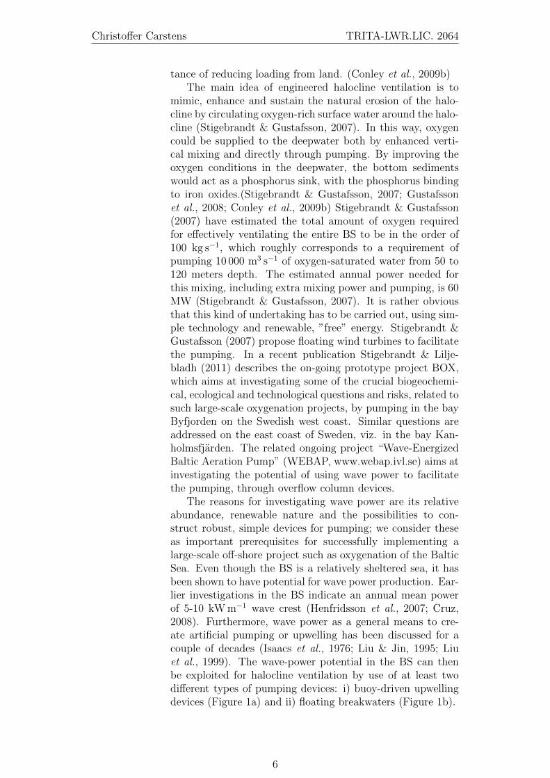
Figure 5: The main fracture zones of Forsmark andtheir transmissivity values.

mainly consisting of the overlying quaternary deposits, thegroundwater surface is highly correlated to the topography.Another system is found in the underlying bedrock, wherethe groundwater pressure generally coincides with a tectoniclens. (Johansson, 2008; Lindborg, 2008)

Data has been extensively collected, through numerouslong term surveying. For this study, a detailed digital eleva-tion model with a resolution of 20 meters, a fracture zone net-work of the large-scale hydrogeological features in the bedrock(Figure 5) and data from flow measurement stations in streams(named PFM) and groundwater level wells (named SFM) havebeen used for model set-up and calibration.

The numerical model built up for DT consists of severalhydrological units. The overburden is conceptualized as alayer of uniform depth with an exponentially decreasing hy-draulic conductivity in the vertical direction, to a minimumvalue, Ksoil = 10−6 m s−1.

Ksoil(d) = Ktop10−d/3 ; if Ksoil ≥ 10−6, (27)

where d is the depth from the soil surface and Ktop is set to5 · 10−3 m s−1. In practice this means that the effective soillayer in the model is approximately 8 meters thick.

The bedrock consists of the known, deterministic fracturezone domain (Figure 5), one stochastic domain of smaller frac-tures and the matrix. (Follin, 2008)

The numerical model consists of a domain with the outerlimits as defined in figure 4 and vertically constrained by thesoil surface and 100 meters depth. Streams and lakes are rep-resented as highly conductive volumes in the domain. Thedomain is discretised in an unstructured Cartesian grid with

15


Figure 6: A detail of the unstructured grid, showingthe finer details around streams, lakes and the coastline.

Figure 7: A 3D illustration of the computationalgrid and permeability. The finer resolution in thetop layer is clearly visible as well as the fracturenetwork in the bedrock regions.

16


Table 1: Grid discretisation scheme. All numbersare in meters. There is also a smoothing effect in thegrid generation, producing a continuous transitionbetween grid sizes. See figure 6.

∆x ∆y ∆z

Bedrock 128 128 8

Soil overburden 32 32 1

Coast 16 16 1

Stream 2 2 1

Lake 2 2 1

Table 2: The different source areas. Position of thelower left corner (LLC) of the square, size of thesource and number of particles (nbp) injected.

Case LLC (X;Y) area nbp

A N/A N/A 5169

B (9000;5000) 1 km2 160

C (2000;6000) 1 km2 125

D (7000;4000) 4 km2 623

E (4000;6000) 4 km2 561

smaller cell sizes around details, such as streams, lakes and thecoastline. In total the computational grid consists of 951 887cells. (Table 1 and Figure 6) The stochastic fracture net-work is generated, using l = 128 m, dl = 372 m, I = 0.2,lref = 1 m. These values generated a total number of 236 942fractures. A 3D illustration of the grid and the conductivedomain shows that the fractures produce conductive zones inthe bedrock (Figure 7). The forcing used to solve the station-ary groundwater level and flow field is a constant infiltrationrate of P − E = 150 mm yr−1.

Deterministic transport times are calculated by using par-ticle tracking through a stationary flow solution. Five dif-ferent cases (A-E) are studied, where source location and sizewere varied from the whole surface of the domain to quadraticsources of 1 km2 size. (Table 2) For all cases the sea has beenfunctioning as a control plane (CP), ensuring that mass break-through is registered for diffuse loading along the whole shoreline. Two special cases are then studied more thoroughly; Aand B, the introduced particles in the whole domain and thesmall source close to the coast. All particles are introduceda certain distance from details, such as stream, lakes and thecoastline. This means that the modelled travel times are allconditional on the injection in the soil domain, which gives abias towards longer transport times on one hand but repre-sents the nature of diffuse sources as transport of e.g nutrientson the other hand.

17


Figure 8: Station names, locations, measurement periods and de-vice names of the SMHI wave measurement stations in the BalticProper basin. The figure also shows the extent of hypoxic zones in2010 (modified from SMHI).

Wave power and floating breakwaters

Wave data from four available wave measurement stations ofthe Swedish Meteorological and Hydrological Institute (SMHI)was analysed to quantify the wave fields and wave power po-tential in the Baltic Proper basin (Figure 8). The data in-cludes one-hour time interval series of significant wave height(Hs) and mean wave period (T). The functionality of the buoy-driven upwelling device will be assessed through calculation ofthe linear wave power from the data, whereas the overtoppingflow will be calculated through relations derived by Frigaardet al. (2004b).

Calculation of linear wave power for buoy clusters

To estimate the number of devices needed it is assumed thatbuoys are able to capture most of the available linear wavepower (in W m−1) if deployed in circular clusters as in theanalysis of Bernhoff et al. (2006). One single cluster contains389 individual devices and has a diameter of 600 m. Thistype of set-up is assumed to be able to capture most of theenergy in incoming wave fronts. We calculate the linear wavepower from the available wave data, seeking the total numberof devices required to produce the needed 60 MW from theavailable waves. The power per meter wave crest, the linearwave power, P [W m−1] is calculated as

P = cgE (28)

where cg is the wave group velocity in m s−1, E is the en-ergy density in J m−2. The group velocity, cg, is calculatedassuming linear wave theory and deep water wave conditions

18


as

cg =gT

4π(29)

where T is the wave period and g is the gravitational acceler-ation. E is related to the significant wave height, Hs, throughthe surface displacement, η [m]

E = ρwg〈η2〉 (30)

where

Hs = 4(〈η2〉

)1/2(31)

This results in an expression of the linear wave power

P = cgE =g2ρwTH

2s

64π(32)

where ρw is the water density (set to 1007 kg m−3, representingtypical Baltic Proper conditions).

Calculation of overtopping flow rates

Overtopping flow capacities of waves on offshore structures isnot a well-documented field. For this study, we have used asuggested expression from the above-mentioned Wave Dragonproject for a linear breakwater with 45 degrees slope (Frigaardet al., 2004b):

q = 0.017cd exp

(−48

Rc

Hc

√Sop2π

)·√gH3

s√Sop

2π

L (33)

where q is the overtopping flow rate in m3 s−1, cd = 0.9 is areduction coefficient for spreading effects, L is the length ofthe breakwater ramp (L = 1 m to calculate specific discharge),Sop = Hs/Lop where is a steepness factor, Rc is the crestfreeboard height, and Tp is the peak wave period calculatedas 1.2T . The overtopping discharge results are sensitive to thechosen freeboard height. For the current study, a freeboardheight of Rc = 0.4 m was chosen as an example.

Results

Modelling of fluxes and transport times

Calibration

The groundwater model is calibrated by ensuring that thegroundwater level corresponds to the large-scale topographicfeatures as indicated by litterature (Johansson (as indicated

19


Table 3: Calibration results for flow. The intervalof measured values indicate the different means forfour different time series. (Johansson, 2008)

Location X Y Simulated [l s−1] Measured [l s−1]

PFM005764 5659 6747 33 25-33

PFM002667 5594 6264 13 12-17

PFM002668 6066 5476 7 9-12

PFM002669 3379 7044 17 12-16

Figure 9: Modelled groundwater levels in Forsmark.The groundwater surface follows the large-scale to-pographic features (Figure 4) The four wells thatthe model reproduce less well (SFM0004-06,09 and0106) are coloured in red with black edges.

20


by 2008)). Where possible, calibration is made against dataof mean groundwater levels in 39 groundwater wells (Figure9, Table 4) and flow rates in streams with time series of flowrates (Figure 3). Most of the values are in good agreement,whereas some show deviations (mainly the wells SFM0004,SFM0005, SFM0006, SFM0009 and SFM0106). Given themany uncertainties in these kinds of modelling and the objec-tive of the current study to exemplify how to combine differentmodelling efforts, and not to show a fully calibrated model,the solution has been considered agreeable.

Basic configuration

The distributions of mean travel times, τi, from the groundwa-ter model indicate asymmetric forms, reflecting the differentflow paths of the different source sizes and locations. (Figure10, 11 and Table 5). PDFs of the mean travel time distribu-tions are difficult to obtain directly from the model results,due to the discrete nature of the modelled CDFs. Slightlymodified distributions that are thought to represent the de-terministic distributions are calculated by summation of equa-tion (20) with α = 0.5 and ζ = 0.3 (Figure 12). These sym-metric and low values of dispersion acts more as a filter onthe deterministic PDF, producing smooth, continuous distri-butions, without changing it significantly, except in the mostextreme cases. The complex and, from commonly used sta-tistical distributions, different shape of the PDFs for the dif-ferent source cases are quite apparent. The PDFs are highlyskewed (Table 5) and in some cases multimodal (Figure 12).

The poor representation of the MRT (¯τ) as a general catch-ment descriptor, is also clearly shown, for example by thecomparison of the mean and the median. The last column intable 5 shows that for all five cases the MRT corresponds tothe time for 80-85 % breakthrough of mass.

Effects of source scale and position

Generally, the source scale (area) influences the shape of thedistribution (Figure 12). Although not unequivocal, increasein source size seems to increase the irregularity of the differ-ent modelled distributions. Multimodality is also present andimportant in e.g. case A and E. This result can be explainedby the fact that larger sources captures more of the hetero-geneity of the catchment, both in terms of pathway lengthand structural differences.

The source distance to the coast or streams is reflected inthe mean travel time (¯τ) and the effect of proximity to streamsin the early arrivals (τ1). (Table 5, Figure 11 and 12) For ex-ample, case E (purple colour), which is both close to the coastand most particles are released relatively close to a stream orlake, shows both a shift towards shorter mean travel times and

21


Table 4: Calibration results for groundwater levelsfor 39 groundwater wells (Figure 9). The four wellsthat the model reproduce less well (SFM0004-06,09and 0106) are coloured in red with black edges.

Well X Y measured simulated ∆

SFM0001 5335 7713 0.5 0.9 0.4

SFM0002 5378 7586 1.2 1.2 -0.1

SFM0003 5487 7615 1.2 1.1 -0.1

SFM0004 7441 6866 2.9 0.7 -2.2

SFM0005 7252 6648 4.9 1.7 -3.2

SFM0006 8502 5747 4.6 1.8 -2.7

SFM0008 8623 5931 0.5 1.3 0.8

SFM0009 7224 6578 4.0 1.6 -2.4

SFM0010 4735 5314 12.5 10.8 -1.8

SFM0011 4711 7117 1.9 2.1 0.2

SFM0013 5123 6699 1.2 2.0 0.8

SFM0014 5716 5027 5.3 5.4 0.1

SFM0016 6174 4976 5.2 5.2 0.0

SFM0017 6138 4505 5.5 5.5 0.0

SFM0018 5950 4558 5.3 5.3 0.1

SFM0019 6118 5701 3.1 2.5 -0.6

SFM0020 6994 6127 1.4 1.4 0.0

SFM0021 6493 7706 1.0 0.7 -0.3

SFM0026 8152 4703 0.7 0.6 -0.1

SFM0028 7589 6508 0.2 0.1 -0.1

SFM0030 5663 6678 1.1 1.1 0.0

SFM0033 5728 6839 0.5 0.7 0.2

SFM0034 5859 7757 0.5 0.6 0.1

SFM0036 5746 7992 0.3 0.6 0.2

SFM0049 4533 8028 2.3 1.6 -0.7

SFM0057 4949 6980 3.4 2.3 -1.1

SFM0058 5740 7349 1.5 0.9 -0.6

SFM0059 9777 6464 0.1 0.2 0.1

SFM0061 9924 6377 0.0 0.4 0.4

SFM0077 4389 7921 2.7 2.7 0.0

SFM0078 4765 7704 3.5 2.1 -1.4

SFM0079 4568 7691 2.7 2.8 0.0

SFM0084 6406 7868 0.5 0.6 0.0

SFM0091 5491 7746 0.4 0.7 0.3

SFM0095 4438 6018 10.5 10.3 -0.2

SFM0104 5275 7592 1.0 1.2 0.3

SFM0105 6465 7710 1.6 0.7 -0.9

SFM0106 8043 6321 3.0 0.6 -2.4

SFM0107 4769 8187 0.9 0.6 -0.2

22


Figure 10: Trajectories for the different source cases A to E (sub-figures a-e) and 3D structure of pathways (f). There is a maximumof 500, randomly chosen, particles shown for each case.

23


10−1

100

101

102

103

10−4

10−3

10−2

10−1

100

τ [years]

cd

f/ccd

f

ABCDE

Figure 11: CDFs and CCDFs for the deterministic,numerically modelled transport times. The powerlaw dependency in the tails of all cases is strong,whereas the early travel times are quite different be-tween the cases.

Table 5: Statistics of the CDF of mean travel times (τ) of the dif-ferent source cases. The different nature of the source sizes andpositions are quite visible from the higher order moments (vari-ance (s2), skewness (γ1) and kurtosis (γ2)) and the percentiles τx.Interestingly, the huge difference between the mean and median ispresent in all distributions. The mean corresponds to the time for80-86 % of tracer breakthrough (last column, CDF(¯τ)).

¯τ s2 s γ1 γ2 CV τ1 τ10 τ50 τ90 τ99 CDF(¯τ)

A 16.3 7058 84.0 22.4 672 5.16 0.27 1.87 4.56 25.0 194 86%

B 12.1 525 22.9 4.5 28 1.90 1.46 2.54 4.85 25.0 124 80%

C 14.9 808 28.4 4.5 25 1.91 0.87 3.38 5.71 29.5 178 81%

D 15.2 3642 60.4 15.2 292 3.98 1.04 2.19 4.60 24.2 188 85%

E 9.9 736 27.1 8.0 84 2.74 0.23 1.08 3.63 19.4 135 84%

24


10−2

10−1

100

101

102

0

0.02

0.04

0.06

0.08

0.1

0.12

0.14

0.16

0.18

0.2

α = 0.5, ζ = 0.3

t [years]

ccdf

Figure 12: PDFs for low dispersion cases that rep-resent slightly filtered deterministic PDFs. Notethat the shape of the curves seems to deviate morefrom regular distributions with the source shape andsize.

less long-term transport. In case C (red), with a 1 km2 source,located far from the coast, we can see a shift towards longertravel times. However, the mean is not larger, due to the lackof very long and slow pathways. In the last case, B (darkgreen), the 1 km2 source is close to the coast but not withinthe reach of any stream one can see the effects of proximityto the coast by the slightly shorter τ and effects of the diffuseloading in the absence of shorter travel times (τ1=1.46 years).Finally, it is worth to mention the full domain source (case A,blue), where effects of both short-time loading and long-termtransport are present, producing a CDF of a quite peculiarshape. The continuous shift between long-term transport andshort-term transport is markedly pronounced by the deviationfrom the turquoise and green curve (cases B and D) towardsthe purple curve (Figure 11, case E). Thus, the full domainencompasses a more complete representation of travel times,as expected, especially at smaller time scales, whereas the 1km2 sources has steeper curves at the early stages. Howeverthe distributions do not seem to follow any commonly usedstatistical descriptions.

In the tail (Figure 11, CCDF), a power-law dependencyis present in all distributions. The relationship seems to holdfor several orders of magnitude.

25


Table 6: Differences in early and late arrivals dueto non-Fickian transport processes

α ζ ∆τ1 ∆τ10 ∆τ50 ∆τ90 ∆τ99443% 36% 6% 0% 36%

0.2 0.3 343% 28% 5% 3% 49%

0.4 0.3 350% 29% 5% 3% 49%

0.6 0.3 357% 29% 5% 3% 49%

0.8 0.3 379% 28% 5% 2% 50%

0.2 0.5 193% 23% 6% 5% 48%

0.4 0.5 229% 23% 6% 5% 48%

0.6 0.5 264% 24% 6% 4% 49%

0.8 0.5 321% 25% 5% 3% 50%

0.2 1 29% 8% 8% 3% 40%

0.4 1 64% 11% 7% 3% 41%

0.6 1 129% 13% 7% 4% 44%

0.8 1 236% 18% 5% 5% 49%

0.2 1.5 7% 2% 6% 2% 32%

0.4 1.5 21% 5% 6% 2% 34%

0.6 1.5 79% 8% 6% 3% 39%

0.8 1.5 200% 14% 5% 5% 46%

Effects of non-Fickian dispersion

A central question in this section is to exemplify how non-Fickian dispersion interacts with the so called basic config-uration. What parts of the mean travel time distributionsare affected by non-Fickian dispersion and by what types andstrengths of non-Fickian dispersion? When does hydrogeologypredominate over dispersion and vice versa? These questionsare studied through sensitivity analysis, where non-Fickiantransport is characterized by variable α and ζ. Effects on themean travel time distributions are visually studied (Figure13 to figure 16) and quantitatively assessed through compactmeasures of the differences in early and late arrivals betweenthe two source cases A and B (full domain and 1 km2) and dif-ferent nature of transport, expressed as different combinationsof α and β. These differences are illustrated as percentiles ofτ between the cases A and B and parameter settings. The dif-ferences are calculated and normalised by the correspondingpercentile of the deterministic model run as

∆τx =|τAx − τBx |

τAx(34)

Also the differences between the deterministic runs are nor-malised in the same way, i.e.

∆τx =|τAx − τBx |

τAx(35)

26


The calculated percentile differences show both large differ-ences and similarities (Table 6).

PDFs and CDFs of cases A and B with varying α andζ (Figures 13 - 16) as well as normalised differences in per-centiles between the cases and parameters (table 6) revealseveral interesting facts. The large effects of dispersion arepresent in the early arrivals. However, in all cases, the in-troduction of dispersion decreases the differences between thetwo deterministic cases. This is evident from the 1%-percentiledifference, which is lower for all combinations of α and γ thanbetween the modelled cases (first row). The difference be-tween different cases of dispersion and deterministic cases canbe very large though (Figures 13 - 16). Thus, introduction ofdispersion reduces the effects of deterministic differences onone hand but increases the spread in the individual distribu-tions on the other hand.

The effects of different values of ζ are apparent in all cases.Even for large values of α (figures 13d and 14d), i.e. plug-flow, dispersion is present. On the other hand, for low valuesof ζ, (Figures 15a-b and 16a-b), the choice of α is unimpor-tant. However, where dispersion is present, α is important forthe change in the distributions. For larger values (α > 0.8)all curves basically coincides with the deterministic distribu-tions, even for ζ > 1 (Figures 13d and 14d). For lower values(α 6 .4), differences between the distributions are lost whenreaching more dispersion (ζ > 1) (Figures 13a and 14a)

For the large source, the deterministic TTD dominates inthe tail. All curves collapse into one CCDF for all tested αand ζ. For the small source dispersion magnitude, ζ, seemsto have some effect, whereas the form of dispersion, α, seemsto be negligible.

27


10−2

100

102

10−4

10−3

10−2

10−1

100

α = 0.2 0.4 0.6 0.8, ζ = 0.3

t [years]

pdf

a

10−2

100

102

10−4

10−3

10−2

10−1

100

α = 0.2 0.4 0.6 0.8, ζ = 0.5

t [years]

pdf

b

10−2

100

102

10−4

10−3

10−2

10−1

100

α = 0.2 0.4 0.6 0.8, ζ = 1

t [years]

pdf

c

10−2

100

102

10−4

10−3

10−2

10−1

100

α = 0.2 0.4 0.6 0.8, ζ = 1.5

t [years]

pdf

d

Figure 13: PDFs when varying α. Dotted: α = 0.2,Dash-dotted: α = 0.4, Dashed: α = 0.6, Solid: α =0.8

10−1

100

101

102

103

10−2

10−1

100

α = 0.2 0.4 0.6 0.8, ζ = 0.3

t [years]

cd

f/ccd

f

a

10−1

100

101

102

103

10−2

10−1

100

α = 0.2 0.4 0.6 0.8, ζ = 0.5

t [years]

cd

f/ccd

f

b

10−1

100

101

102

103

10−2

10−1

100

α = 0.2 0.4 0.6 0.8, ζ = 1

t [years]

cd

f/ccd

f

c

10−1

100

101

102

103

10−2

10−1

100

α = 0.2 0.4 0.6 0.8, ζ = 1.5

t [years]

cd

f/ccd

f

d

Figure 14: CDFs and CCDFs when varying α. Dot-ted: α = 0.2, Dash-dotted: α = 0.4, Dashed: α =0.6, Solid: α = 0.8

28


10−2

100

102

10−4

10−3

10−2

10−1

100

α = 0.2, ζ = 0.3 0.5 1 1.5

t [years]

pdf

a

10−2

100

102

10−4

10−3

10−2

10−1

100

α = 0.4, ζ = 0.3 0.5 1 1.5

t [years]

pdf

b

10−2

100

102

10−4

10−3

10−2

10−1

100

α = 0.6, ζ = 0.3 0.5 1 1.5

t [years]

pdf

c

10−2

100

102

10−4

10−3

10−2

10−1

100

α = 0.8, ζ = 0.3 0.5 1 1.5

t [years]

pdf

d

Figure 15: PDFs when varying ζ Dotted: ζ = 0.3,Dash-dotted: ζ = 0.5, Dashed: ζ = 1, Solid: ζ = 1.5

10−1

100

101

102

103

10−2

10−1

100

α = 0.2, ζ = 0.3 0.5 1 1.5

t [years]

cd

f/ccd

f

a

10−1

100

101

102

103

10−2

10−1

100

α = 0.4, ζ = 0.3 0.5 1 1.5

t [years]

cd

f/ccd

f

b

10−1

100

101

102

103

10−2

10−1

100

α = 0.6, ζ = 0.3 0.5 1 1.5

t [years]

cd

f/ccd

f

c

10−1

100

101

102

103

10−2

10−1

100

α = 0.8, ζ = 0.3 0.5 1 1.5

t [years]

cd

f/ccd

f

d

Figure 16: CDFs and CCDFs when varying ζ. Dot-ted: ζ = 0.3, Dash-dotted: ζ = 0.5, Dashed: ζ = 1,Solid: ζ = 1.5

29


10−2

10−1

100

101

102

0

0.05

0.1

0.15

α = 0.5, ζ = 0.3

t [years]

pd

f10

−210

−110

010

110

20

0.02

0.04

0.06

0.08

0.1

0.12

0.14

0.16

α = 0.5, ζ = 0.5

t [years]

pd

f

10−2

10−1

100

101

102

0

0.05

0.1

0.15

0.2

α = 0.5, ζ = 1

t [years]

pd

f

10−2

10−1

100

101

102

0

0.05

0.1

0.15

0.2

0.25

0.3

α = 0.5, ζ = 1.5

t [years]

pd

f

Figure 17: PDFs when varying ζ and adding masstransfer process

Effects of mass transfer due to molecular diffusion

The effects of microscopic retention are smaller and mainlyemphasised in the peak (Figure 17). Even though these mi-croscopic mobilisation-immobilisation processes occur on verylong time-scales the effect is pronounced in the peak. Thepresence of molecular mass transfer effects on these PDFsis interesting, due to the fact that even conservative tracershave different diffusion coefficients. This indicates that theremight be differences between different tracers, that should beaccounted for, at least in long-term modelling.

Wave-powered aeration in the Baltic Sea

Statistics of wave data for each station and the full dataset,shows skewed statistics and a relatively large difference be-tween the single offshore station in the Baltic Proper (stationSodra Ostersjon (Figure 8) and the 3 coastal stations. (Table7) For the whole dataset, mean Hs is 1.01 m and mean T is4.0 s. Calculations of wave power and overtopping flow ratesare solely dependant on this data and the differences betweenstation are only amplified (Table 8). In both analyses the50 to 90 percentiles are assumed to represent the uncertaintybounds for available average energy.

Linear wave power and buoy clusters

Figure 18a illustrates the statistical distribution of calculatedwave power, P , which is needed for estimating the buoy device

30


(Figure 1a) requirements. The 50 to 90 percentile interval ofcalculated P from all the available wave data series is 1.2 to10.1 kW m−1, with the mean at 4.0 kW m−1. The previouslyestimated values of 5 to 10 kW m−1 for the BS (Henfridssonet al., 2007; Cruz, 2008) correspond to the higher-value partof the power distribution found in this study. This might beexplained by the near-coastal bias in the dataset. Simulationsof the wave fields for the whole Baltic Proper basin (Jonssonet al., 2003) indicate a more intense overall wave climate thanin the coastal waters. The mean significant wave heights maybe substantially greater in the central Baltic Proper, than inthe coastal part of the BS, which is indicated by the datafrom Sodra Ostersjon. These show 25 percent higher valuesfor Hs and around 50 percent higher values for P compared tototal statistics (Tables 7 and 8). This also strengthen such in-ference, implying that the 50-90 percentile interval suggestedhere is relevant, and more likely to under- than over-estimatethe available wave power, as indicated in figure 18a.

The 50 to 90 percentile wave power range of 1.2 to 10.1kW m−1 implies that 5.9 to 50 km of wave crest must be cap-tured to fulfil the total mean annual power requirement of60 MW (Stigebrandt & Gustafsson, 2007). Using a set-up of389 buoys that form circular clusters with diameters of 600meters (as suggested for utilization of wave energy resourcesin sheltered sea areas (Bernhoff et al., 2006), 10 to 83 suchbuoy parks would suffice to meet the total power need of 60MW. The occupied area of each cluster would then be around0.28 km2, roughly corresponding to 40 soccer fields (one soc-cer field = 7140 m2), and the total area for all clusters wouldbe in the range 2.8 to 23 km2. This corresponds to 12 to 100ppm of the Baltic Proper and 7-55 ppm of the whole BS area.

Floating breakwaters and overtopping flow rates

For the estimation of the breakwater device (Figure 1a) re-quirements, figure 18b shows the data-based statistical distri-bution of the flow, q, overtopping an example crest freeboardheight of 0.4 m. The 50 to 90 percentile of q is 0.12 to 0.93m3s−1m−1 with a mean of 0.34 m3s−1m−1. This q intervalimplies a required total breakwater length in the range of 11to 83 km in order to meet the total flow requirement of 10 000m3s−1m−1. In analogy with the wave power calculations forthe buoy devices, the distribution for q is expected to be evengreater in the sea. The q-values for Sodra Ostersjon are cal-culated to be around 40 percent higher than for the data setin total. (Table 8 and Figure 18b )

31


Table 7: Statistics of main wave parameters for the different mea-surement stations and all stations combined (row All). H is givenin [m] and T in [s].

Mean H MedianH

90%-H Mean T MedianT

90%-T

Almagrundet 0.93 0.70 1.92 3.99 3.80 5.20

Huvudskar 0.99 0.84 1.88 3.90 3.74 5.04

Olands sodra grund 1.03 0.85 1.99 4.04 3.90 5.30

Sodra Ostersjon 1.25 1.05 2.51 3.98 3.85 5.45

All 1.01 0.80 2.01 4.00 3.80 5.30

Table 8: Results for wave energy propagation and calculated over-topping rates for each wave station and all stations combined (rowAll). Notice the significantly higher values in the Sodra Ostersjonbuoy, which is located in the open sea, compared to the other, near-coastal wave stations. P is given in [kWm−1] and q in [m3s−1m−1].

Mean P MedianP

90%-P Mean q Medianq

90%-q

Almagrundet 3.66 0.90 8.96 0.31 0.09 0.83

Huvudskar 3.27 1.26 8.50 0.29 0.12 0.80

Olands sodra grund 3.90 1.35 10.02 0.35 0.14 0.95

Sodra Ostersjon 5.92 1.91 15.90 0.47 0.18 1.30

All 3.98 1.19 10.07 0.34 0.12 0.93

Figure 18: a) Cumulative distributions of linear wave power andb) overtopping flow rate distributions. Results shown in a) and b)are calculated from the same wave data. Notice the shift towardshigher values in the data from the sole off-shore station SodraOstersjon.

32


Discussion

Transport time modelling

The objectives of the transport study have been to i) presenta case on how to combine different modelling approaches (nu-merical, physically based and semi-analytical, stochastic) toinclude effects of dispersion in different space and time scalesand of different origin, such as geological, hydrodynamic, dif-fusive, etc., ii) investigate the importance and influence ofsource size and position on the mean travel time distributions,iii) describe and illustrate how non-Fickian dispersion relatesand alters the effects of source size, and iv) address questionsof how mass transfer processes alters the travel time distribu-tions.

We have shown and exemplified a framework for how dis-tributed, large scale and very detailed, physically based mod-els can be linked to stochastic, Lagrangian modelling tech-niques. The framework is efficient in the sense that it capturesdispersion on all scales; macro-dispersion (geomorphological,geological) of large-scale structures through the use of deter-ministic TTDs and meso-scale dispersion (hydrodynamic) inthe use of statistical TTDs conditioned on the modelled meantravel times and small-scale micro-dispersion and retention inthe inclusion of the memory function. Since the determinis-tic model can require substantial computational power (up toweeks for stable solutions), this is a feasible way of includinguncertainty in physically based modelling.

The relatively late first arrivals of the smaller source caseindicate an important factor when dealing with transportfrom diffuse but geographically confined sources. Early ar-rivals that are present in commonly used statistical distribu-tion functions might not be present if there is a relatively longdistance to the nearest stream.

MRT (¯τ) is problematic as a catchment descriptor, dueto the heavy skewness and multi-modal nature of the TTDs.In all of our cases the MRT corresponds to 80-85% of massbreakthrough, rather than the median. This means that usingthe mean as a value for flushing of contaminants will greatlyoverestimate the time the bulk will stay in the system. Thisissue has earlier been discussed in stream water and transientstorage zones by Runkel (2002), who propose the median asa better transport metric.

The multimodal shape of the BTC also effectively illus-trates the difficulty in choosing proper statistical distributionsfor real-life applications. This in turn gives implications onthe common practice for data fitting and convolution integraltechniques. If the range of possible distributions is large andnot defined by analytical expressions, one can argue that theinsight commonly used statistical distributions (McGuire &

33


McDonnell, 2006) gives on catchment behaviour is limited.Introduced local variability on the deterministic transport

times alters the distributions as shown in figures 13 - 16. Mostimportantly, the general shape of the deterministic distribu-tions prevail for relatively high orders of dispersion. For exam-ple, the multimodality of case A is smoothed out but presentin almost all cases. The geomorphological part of dispersionis strong as concluded earlier Rinaldo et al. (e.g. by 1991).The magnitude of dispersion, expressed as the coefficient ofvariation, ζ, exercises first-order control on hydrodynamic,or local dispersion, in the sense that moderately high valuesζ > 0.75 are needed to alter the distributions at significantly.α exercises second-order control. However, when dispersionis large enough to alter the deterministic distributions, α isdecisive for the way the distribution is changed. α > 0.5does not really change the form of the distribution, but onlygives rise to a shift towards earlier arrivals. α < 0.5 on theother hand both smooths the deterministic features and heav-ily raises the probability for early arrivals. In summary, thismeans that systems of low dispersion are not subject to largechanges of the deterministic travel time distributions, regard-less of the nature of the dispersion. However, when dispersionincreases, α is decisive for the way dispersion is altering thedistributions.

Introduction of dispersion gives a higher probability ofearly arrivals but it also decreases the relative differences be-tween early arrivals of source-dependent cases.

For large source, the deterministic TTD dominates in thetail. For the small source dispersion magnitude, ζ, seems tohave some effect, whereas the form of dispersion, α, seems tobe less important. Earlier studies (Riml & Worman, 2011)have shown an increase in the importance of the hydraulicdispersive term when going from diffuse loadings to pointsources, which could be supported by this study in the sensethat for diffuse and large sources the deterministic featuresseems to be more prevailing.

A power-law dependency in the distribution tails is evidentfor all sizes of sources but is more pronounced in the full-domain source case.

Introduction of retention and molecular mass transfer in-duce effects on the TTD, especially in combination with non-Fickian transport and at the peaks of the PDFs. This mightbe important in cases, when using multiple tracer data. Evenso-called conservative tracers are subject to mass transfer pro-cesses and diffusion and might thus have different travel timedistributions that should be accounted for.

34


Wave-powered halocline ventialtion

Costs and feasibility

For both types of wave power devices, the total requirementsin terms of number of devices, could be argued to fall withina technically reasonable and feasible range. With regard toeconomic feasibility, the pipe material cost of a single buoypump is estimated to about 18 000 EUR (for pipes of 60 m ata cost of 300 EUR per m). Doubling this cost to account alsofor additional material, work and mooring costs, yields a totaldevice cost of 36000 EUR. The total cost for 10-83 clusterswould then be 136 to 1 132 million EUR. For the alternativeuse of 50 m long breakwater devices, the required total lengthof 11 to 83 km implies 220 to 1 660 devices. Estimating adevice material cost of 300 000 EUR (for 80 m pipes and 2500m3 of concrete) and doubling that to account also for trans-portation and mooring costs, yields the total cost range of 132to 996 million EUR. These are not unreasonable costs, for in-stance relative to estimated BASP implementation costs Gren(2008); Gren et al. (2008), or to other proposed engineeredmeasures for BS remediation. The cost for chemical phospho-rus sequestration of the whole BS water volume, for example,has been estimated to 1-3 billion EUR Blomqvist & Rydin(2009). Stigebrandt & Gustafsson (2007) calculates (very op-timistically) the cost for facilitating halocline ventilation bythe use of floating wind turbines to 200 million EUR.

Technological advantages

In comparison to previously proposed wind-powered pump-ing devices for halocline ventilation Stigebrandt & Gustafs-son (2007), there are several technical advantages of usingthe wave-powered systems proposed here. The wave devicesinvolve existing, proven and relatively simple technological so-lutions. Both device types use few moving parts, comparedto the quite complex engineering requirements for floatingwind turbines. Even though the wave-powered devices mustbe able to withstand rough offshore conditions, these sim-ple, low structures are likely to be more robust and reliablethan higher floating windmills. The large torque that float-ing wind mills would be subjected to during operation is alsoa constructional challenge that makes the technological andcost estimates quite uncertain; in spite of some recent re-search, the use and durability of floating wind turbines is stillin its infancy. By contrast, buoys and floating breakwatersare demonstrated devices for pumping and overflow columns,that should be relatively easily adopted for the specific taskof halocline ventilation.

35


Open issues

There remain many important open questions concerning theproposed measures that should be focus of future and on-going research. The assumed effects from the original methodof halocline ventilation are still untested in-situ (except forthe naturally occurring experiment during the mid-90s Stige-brandt & Gustafsson (2007)). The ecological effects of dif-ferent proposed measures have to be investigated further. Infact, a handful of projects (WEBAP1, BOX2, PROPPEN3)are at present studying effects of pumping water from severaldepths in the Baltic Sea; results from those projects, expectedin the near future, will further expose the limitations and po-tential risks with halocline ventilation methods.

Conclusions

Transport modelling in near-coastal catchments

This part of the study has been motivated by the need ofquantification of transport processes and effects on tracerswithin catchments. Catchments in general and near-coastalcatchments in particular are often lacking data or very diffi-cult to monitor. The monitoring problem applies to forcings,processes and discharges of both water and tracers. This callsfor system understanding and methodologies to combine dis-tributed modelling of water movement with analytical toolsfor transport processes and transformations. The study shows(i) A straightforward framework for combining physically-based modelling with Lagrangian methods has been presented.(ii) Catchment travel time distributions as well as tracer traveltime distributions from sources of different sites exhibit com-plex forms. (iii.) Effects of Fickian and non-Fickian transportis shown to alter the travel time distributions but the maindifferences between the source cases prevail for small to mod-erate dispersion intensity (coefficient of variation, ζ < 1).

Further studies are needed to develop methods to resolveissues on where and how to emphasise nutrient loading reduc-tion programs to recipients, both in terms of source reduc-tions and in-situ abatement measures and the combinationsof these. Cost-efficient measures use combinations of differentmethods and at optimised locations within catchments andrecipient. This requires methodologies to asses these complexinteractions, spatially and temporally within feasibly simpleframeworks.

The effects of hydrogeological structures and conceptualmodels have been shown to influence the travel time distri-

1http://webap.ivl.se2http://www.marsys.se/3http://www.miljo.fi/syke/proppen

36


butions of analytical expressions. To better distinguish thesources of dispersion and to quantify their relative impor-tance, in relation to local, or small-scale, heterogeneity andmass transfer effects would be a goal of the further studies.

Inclusion of tracer transport data in the modelling frame-work is another area that would provide insight and knowledgeto process understanding. The framework itself provides thetools for process separation but spatially distributed time se-ries of multiple tracer data is the key for both deeper processunderstanding and real-life applied studies.

The latest point leads to another question of further stud-ies; effects of transients. The current study has been restrictedby assumptions on stationary flow conditions. Inclusion ofdata requires methodologies to handle transients. The an-alytical framework can handle time-variant velocity magni-tudes (but not directions) (Cvetkovic et al., 2012) but thereremain several questions on how to deal with transient forc-ings, sources, TTDs and mass transfer processes.

Wave-powered halocline ventilation

This part of the study has been motivated by three facts: (i)The problem of eutrophication in the BS, as well as worldwide,has complex causes and a history over many decades; anysustainable solution to the problem must be based on reducingoverall external and internal loadings of nutrients to the sea.(ii) Large-scale engineered halocline ventilation is a means ofmimicking a natural process of intermittent halocline mixing,with the purpose of reducing hypoxia and associated internalnutrient loadings. (iii) Relatively simple technology can beused to harness wave power for halocline ventilation. Thepresent results have shown that it is both technologically andeconomically feasible to harness sufficient wave power for therequired halocline ventilation for mitigating the BS hypoxia.

Further investigations (several of which are underway) areneeded to resolve whether, where and under what conditionsthe proposed wave-power methods are cost-efficient and eco-logically sustainable for large-scale halocline ventilation, andto optimize them for such use, separately or in combinationwith other possible measures for hypoxia mitigation. Thisstudy has shown that wave-power methods could indeed befeasible, at least in terms of energy availability, for mitigationof hypoxia in the Baltic Sea, and possibly for other hypoxiccoastal and marine environments. Future studies should bemade on the robustness and efficiency of the different pump-ing technologies and the internal behaviour of recipients tobetter assess the efficiency of such devices.

37


Linking the two

The final step of the future studies would be to relate thedifferent options for combating eutrophication to each other.An effort to link processes and measures in catchments; loadreductions, transport processes and measures within the hy-drological system (in the virtual pipe), with possibilities toreduce effects in the recipients (at the end of the virtual pipe)would be the final aim of this study.

38


References

Backer, H. & Leppanen, J.M. (2008). The HELCOM system of a vision, strate-gic goals and ecological objectives: implementing an ecosystem approach tothe management of human activities in the Baltic Sea. Aquatic Conservation:Marine and Freshwater Ecosystems, 18(3):321–334. doi:10.1002/aqc.851.

Bernhoff, H., Sjostedt, E. & Leijon, M. (2006). Wave energy resources insheltered sea areas: A case study of the Baltic Sea. Renewable Energy,31(13):2164 – 2170. doi:10.1016/j.renene.2005.10.016.

Beven, K.J. (1989). Changing Ideas in Hydrology - the Case of Physically-based Models. Journal of Hydrology, 105(1-2):157–172.

Beven, K.J. (2001). Dalton Medal Lecture: How far can we go in distributedhydrological modelling? Hydrology and Earth System Science, 5(1):1–12.

Bindler, R., Renberg, I., Rydberg, J. & Andren, T. (2009). Widespread wa-terborne pollution in central Swedish lakes and the Baltic Sea from pre-industrial mining and metallurgy. Environmental Pollution, 157(7):2132–2141. doi:10.1016/j.envpol.2009.02.003.

Blomqvist, S. & Rydin, E. (2009). Hur fosforbindningen i Ostersjonsbottensediment kan forstarkas. Technical Report 5914, Natuvardsverket(Swedish EPA).

Botter, G., Bertuzzo, E. & Rinaldo, A. (2010). Transport in the hydro-logic response: Travel time distributions, soil moisture dynamics, andthe old water paradox. Water Resources Research, 46:W03514. doi:10.1029/2009WR008371.

Branvall, M., Bindler, R., Emteryd, O. & Renberg, I. (2001). Four thousandyears of atmospheric lead pollution in northern Europe: a summary fromSwedish lake sediments. Journal of Paleolimnology, 25(4):421–435. doi:10.1023/A:1011186100081.

Breivik, K., Sweetman, A., Pacyna, J.M. & Jones, K.C. (2002). Towards aglobal historical emission inventory for selected PCB congeners — a massbalance approach: 1. Global production and consumption. Science of TheTotal Environment, 290(1–3):181–198. doi:10.1016/S0048-9697(01)01075-0.

Conley, D.J., Bjorck, S., Bonsdorff, E., Carstensen, J., Destouni, G., Gustafs-son, B.G., Hietanen, S., Kortekaas, M., Kuosa, H., Markus Meier, H.E.,Muller-Karulis, B., Nordberg, K., Norkko, A., Nurnberg, G., Pitkanen, H.,Rabalais, N.N., Rosenberg, R., Savchuk, O.P., Slomp, C.P., Voss, M., Wulff,F. & Zillen, L. (2009a). Hypoxia-Related Processes in the Baltic Sea. Envi-ronmental Science & Technology, 43(10):3412–3420. doi:10.1021/es802762a.

Conley, D.J., Bonsdorff, E., Carstensen, J., Destouni, G., Gustafsson, B.G.,Hansson, L.A., Rabalais, N.N., Voss, M. & Zillen, L. (2009b). Tackling Hy-poxia in the Baltic Sea: Is Engineering a Solution? Environmental Science& Technology, 43(10):3407–3411. doi:10.1021/es8027633.

39


Conley, D.J., Carstensen, J., Aigars, J., Axe, P., Bonsdorff, E., Eremina, T.,Haahti, B.M., Humborg, C., Jonsson, P., Kotta, J., Lannegren, C., Larsson,U., Maximov, A., Medina, M.R., Lysiak-Pastuszak, E., Remeikaite-Nikiene,N., Walve, J., Wilhelms, S. & Zillen, L. (2011). Hypoxia Is Increasing inthe Coastal Zone of the Baltic Sea. Environmental Science & Technology,45(16):6777–6783. doi:10.1021/es201212r.

Conley, D.J., Paerl, H.W., Howarth, R.W., Boesch, D.F., Seitzinger, S.P.,Havens, K.E., Lancelot, C. & Likens, G.E. (2009c). Controlling Eutroph-ication: Nitrogen and Phosphorus. Science, 323(5917):1014–1015. doi:10.1126/science.1167755.

Cruz, J. (2008). Ocean wave energy: current status and future prepectives.Springer, 93-133 pp.

Cvetkovic, V.D. (2011). The tempered one-sided stable density: a univer-sal model for hydrological transport? Environmental Research Letters,6:034008. doi:10:1088/1748-9326/6/3/034008.

Cvetkovic, V.D. (2011). Tracer attenuation in groundwater. Water ResourcesResearch, 47:W12541. doi:10.1029/2011WR010999.

Cvetkovic, V.D., Carstens, C., Selroos, J.O. & Destouni, G. (2012). Water andsolute transport along hydrological pathways. Water Resources Research. (inreview).

Cvetkovic, V.D. & Dagan, G. (1994). Transport of kinetically sorbing soluteby steady random velocity in heterogeneous porous formations. Journal ofFluid Mechanics, 265:189–215.

Cvetkovic, V.D. & Haggerty, R. (2002). Transport with multiple-rateexchange in disordered media. Physical Review E, 65:051308. doi:10:1103/PhysRevE.65.051308.

Dagan, G. (1984). Solute Transport in Heterogeneous Porous Formations.Journal of Fluid Mechanics, 145:151–177.

Dagan, G., Cvetkovic, V.D. & Shapiro, A.M. (1992). A Solute Flux Approachto Transport in Heterogeneous Formations 1. The General Framework. Wa-ter Resources Research, 28(5):1369–1376.

Darracq, A., Destouni, G., Persson, K., Prieto, C. & Jarsjo, J. (2010). Quan-tification of advective solute travel times and mass transport through hy-drological catchments. Environmental Fluid Mechanics, 10(1-2):103–120.doi:10.1007/s10652-009-9147-2.

Destouni, G., Hannerz, F., Prieto, C., Jarsjo, J. & Shibuo, Y. (2008). Smallunmonitored near-coastal catchment areas yielding large mass loading to thesea. Global Biogeochemical Cycles, 22:GB4003. doi:10.1029/2008GB003287.

Diaz, R.J. & Rosenberg, R. (2008). Spreading Dead Zones and Con-sequences for Marine Ecosystems. Science, 321(5891):926–929. doi:10.1126/science.1156401.

40


Dincer, T., Payne, B.R., Florkowski, T., Martinec, J. & Tongiorgi, E. (1970).Snowmelt runoff from measurements of tritium and oxygen-18. Water Re-sources Research. doi:10.1029/WR006i001p00110.

Dunn, S.M., Birkel, C., Tetzlaff, D. & Soulsby, C. (2010). Transit time distri-butions of a conceptual model: their characteristics and sensitivities. Hy-drological Processes, 24(12):1719–1729. doi:10.1002/hyp.7560.

Elmgren, R. & Larsson, U. (2001). Science and Integrated Coastal Manage-ment, chapter Eutrophication in the Baltic Sea area. Integrated coastal man-agement issues. Berlin: Dahlem University press.

Fiori, A. & Russo, D. (2008). Travel time distribution in a hillslope: Insightfrom numerical simulations. Water Resources Research, 44(12):W12426.doi:10.1029/2008WR007135.

Follin, S. (2008). Bedrock hydrogeology Forsmark. Site descriptive modelling,SDM-Site Forsmarkk. Technical Report R-08-95, Swedish Nuclear Fuel andWaste Management Co.

Frigaard, P., Kofoed, J.P. & Knapp, W. (2004b). Wave Dragon. Wave PowerPlant using Low-head Turbines. In: Conference Report: Hidroenergia 2004- International Conference and Exhibition on Small Hydropower.

Frigaard, P., Kofoed, J.P. & Rasmussen, M.R. (2004a). Overtopping Measure-ments on the Wave Dragon Nissum Bredning Prototype. In: Proceedingsof the The Fourteenth (2004) International Offshore and Polar EngineeringConference, J.S. Chung, K. Izumiyama, M. Sayed & S.W. Hong, eds., vol-ume 1, pp. 210–216. International Society of Offshore and Polar Engineers(ISOPE).

Galloway, J.N., Townsend, A.R., Erisman, J.W., Bekunda, M., Cai, Z., Freney,J.R., Martinelli, L.A., Seitzinger, S.P. & Sutton, M.A. (2008). Transforma-tion of the Nitrogen Cycle: Recent Trends, Questions, and Potential Solu-tions. Science, 320(5878):889–892. doi:10.1126/science.1136674.

Galloway, J. & Cowling, E. (2002). Reactive nitrogen and theworld: 200 years of change. Ambio, 31(2):64–71. doi:10.1639/0044-7447(2002)031[0064:RNATWY]2.0.CO;2.

Galloway, J., Dentener, F., Capone, D., Boyer, E., Howarth, R., Seitzinger,S., Asner, G., Cleveland, C., Green, P., Holland, E., Karl, D., Michaels, A.,Porter, J., Townsend, A. & Vorosmarty, C. (2004). Nitrogen cycles: past,present, and future. Biogeochemistry, 70(2):153–226. doi:10.1007/s10533-004-0370-0.

Godsey, S.E., Aas, W., Clair, T.A., de Wit, H.A., Fernandez, I.J., Kahl, J.S.,Malcolm, I.A., Neal, C., Neal, M., Nelson, S.J., Norton, S.A., Palucis, M.C.,Skjelkvale, B.L., Soulsby, C., Tetzlaff, D. & Kirchner, J.W. (2010). General-ity of fractal 1/f scaling in catchment tracer time series, and its implicationsfor catchment travel time distributions. Hydrological Processes, 24(12):1660–1671. doi:10.1002/hyp.7677.

41


Goltz, M.N. & Roberts, P.V. (1987). Using the method of moments to an-alyze 3-dimensional diffusion-limited solute transport from temporal andspatial perspectives. Water resources Research, 23(8):1575–1585. doi:10.1029/WR023i008p01575.

Gren, I.M. (2008). Cost effectiveness and fairness of the Helcom Baltic SeaAction Plan against eutrophication. Vatten, 64(4):273–281.

Gren, I.M., Jonzon, Y. & Lindqvist, M. (2008). Costs of nutrient reductionsto the Baltic Sea. Technical report, Uppsala:SLU.

Gustafsson, B.G., Meier, H.E.M., Savchuk, O.P., Eilola, K., Axell, L. & Alm-roth, E. (2008). Simulation of some engineering measures aiming at reduc-ing effects from eutrophication of the Baltic Sea. Technical report, Baltic-Sea2020.

HELCOM (2007). The HELCOM Baltic Sea Action Plan. HELCOM.

Henfridsson, U., Neimane, V., Strand, K., Kapper, R., Bernhoff, H., Daniels-son, O., Leijon, M., Sundberg, J., Thorburn, K., Ericsson, E. & Bergman,K. (2007). Wave energy potential in the Baltic Sea and the Danish partof the North Sea, with reflections on the Skagerrak. Renewable Energy,32(12):2069 – 2084. doi:DOI: 10.1016/j.renene.2006.10.006.

Howden, N.J.K., Burt, T.P., Worrall, F., Whelan, M.J. & Bieroza, M.(2010). Nitrate concentrations and fluxes in the River Thames over 140years (1868–2008): are increases irreversible? Hydrological Processes,24(18):2657–2662. doi:10.1002/hyp.7835.

Huisman, J., Matthijs, H.C. & Visser, P.M. (eds.) (2005). Harmful Cyanobac-teria, volume 3 of Aquatic Ecology Series. Springer Dordrecht.

Ibaraki, M. (2001). Source Characteristics and Contaminant Plume Evolution.Transport in Porous Media, 44:577–589. 10.1023/A:1010704406512.

Isaacs, J.D., Castel, D. & Wick, G.L. (1976). Utilization of the energy inocean waves. Ocean Engineering, 3(4):175 – 182, IN3–IN4, 183–187. doi:DOI: 10.1016/0029-8018(76)90022-6.

Jonsson, A., Broman, B. & Rahm, L. (2003). Variations in the Baltic Seawave fields. Ocean Engineering, 30(1):107 – 126. doi:DOI: 10.1016/S0029-8018(01)00103-2.

Johansson, P.O. (2008). Decription of surface hydrology and near-surface hy-drogeology at Forsmark. Technical Report R-08-08, Swedish Nuclear Fueland Waste Management Co.

Kirchner, J.W., Feng, X. & Neal, C. (2000). Fractal stream chemistryand its implications for contaminant transport in catchments. Nature,403(6769):524–527. doi:10.1038/35000537.

Kofoed, J.P. (2002). Wave Overtopping of Marine Structures - Utilization ofWave Energy. Ph.D. thesis, Alborg University, Department of Civil Engi-neering.

42


Kreft, A. & Zuber, A. (1978). On the Physical Meaning of the DispersionEquation and its Solutions for Different Initial and Boundary Conditions.Chemical Engineering Science, 33(11):1471–1480.

Li, L., Barry, D., Stagnitti, F. & Parlange, J. (1999). Submarine groundwaterdischarge and associated chemical input to a coastal sea. Water ResourcesResearch, 35(11):3253–3259. doi:10.1029/1999WR900189.

Lindborg, T. (2008). Surface system Forsmark. Technical Report R-08-11,Swedish Nuclear Fuel and Waste Management Co.

Lindgren, G.A., Destouni, G. & Miller, A.V. (2004). Solute transport throughthe integrated groundwater-stream system of a catchment. Water ResourcesResearch, 40(3):W03511. doi:10.1029/2003WR002765.

Liu, C.C.K., Dai, J.J., Lin, H. & Guo, F. (1999). Hydrodynamic Performanceof Wave-Driven Artificial Upwelling Device. Journal of Engineering Me-chanics, 125(7):728–732. doi:10.1061/(ASCE)0733-9399(1999)125:7(728).

Liu, C.C.K. & Jin, Q. (1995). Artificial upwelling in regular and random waves.Ocean Engineering, 22(4):337 – 350. doi:DOI: 10.1016/0029-8018(94)00019-4.

Maloszewski, P. & Zuber, A. (1982). Determining the turnover time of ground-water systems with the aid of environmental tracers: 1. Models and theirapplicability. Journal of Hydrology, 57(3-4):207–231. doi:10.1016/0022-1694(82)90147-0.

McDonnell, J.J., McGuire, K., Aggarwal, P., Beven, K.J., Biondi, D.,Destouni, G., Dunn, S., James, A., Kirchner, J., Kraft, P., Lyon, S., Mal-oszewski, P., Newman, B., Pfister, L., Rinaldo, A., Rodhe, A., Sayama, T.,Seibert, J., Solomon, K., Soulsby, C., Stewart, M., Tetzlaff, D., Tobin, C.,Troch, P., Weiler, M., Western, A., Worman, A. & Wrede, S. (2010). Howold is streamwater? Open questions in catchment transit time conceptual-ization, modelling and analysis. Hydrological Processes, 24(12):1745–1754.doi:10.1002/hyp.7796.

McGuire, K.J. & McDonnell, J.J. (2006). A review and evaluation of catch-ment transit time modeling. Journal of Hydrology, 330(3-4):543–563. doi:10.1016/j.jhydrol.2006.04.020.

McGuire, K., Weiler, M. & McDonnell, J. (2007). Integrating tracerexperiments with modeling to assess runoff processes and water tran-sit times. Advances in Water Resources, 30(4):824 – 837. doi:10.1016/j.advwatres.2006.07.004.

Moore, W.S. (2010). A reevaluation of submarine groundwater discharge alongthe southeastern coast of North America. Global Biogeochemical Cycles, 24.doi:10.1029/2009GB003747.

Moore, W.S., Sarmiento, J.L. & Key, R.M. (2008). Submarine groundwa-ter discharge revealed by Ra-228 distribution in the upper Atlantic Ocean.Nature Geoscience, 1(5):309–311. doi:10.1038/ngeo183.

43


Moore, W. (1996). Large groundwater inputs to coastal waters revealed byRa-226 enrichments. Nature, 380(6575):612–614. doi:10.1038/380612a0.

Renberg, I., Bindler, R., Bradshaw, E., Emteryd, O. & McGowan, S. (2001).Sediment evidence of early eutrophication and heavy metal pollution of LakeMalaren, central Sweden. Ambio, 30(8):496–502.

Riml, J. & Worman, A. (2011). Response functions for in-stream so-lute transport in river networks. Water Resources Research, 47. doi:10.1029/2010WR009412.

Rinaldo, A., Marani, A. & Rigon, R. (1991). Geomorphological Dispersion.Water Resources Research, 27(4):513–525. doi:10.1029/90WR02501.

Rinaldo, A., Beven, K.J., Bertuzzo, E., L. Nicotina, J.D., Fiori, A., Russo, D.& Botter, G. (2011). Catchment travel time distributions and water flow insoils. Water Resources Research, 47:W07537. doi:10.1029/2011WR010478.

Rockstrom, J., Steffen, W., Noone, K., Persson, A., Chapin, III, F.S., Lambin,E.F., Lenton, T.M., Scheffer, M., Folke, C., Schellnhuber, H.J., Nykvist, B.,de Wit, C.A., Hughes, T., van der Leeuw, S., Rodhe, H., Sorlin, S., Snyder,P.K., Costanza, R., Svedin, U., Falkenmark, M., Karlberg, L., Corell, R.W.,Fabry, V.J., Hansen, J., Walker, B., Liverman, D., Richardson, K., Crutzen,P. & Foley, J.A. (2009). A safe operating space for humanity. Nature,461(7263):472–475. doi:10.1038/461472a.

Runkel, R.L. (2002). A new metric for determining the importance of transientstorage. Journal of the North American Benthological Society, 21(4):529–543. doi:10.2307/1468428.

Stigebrandt, A. & Gustafsson, B.G. (2007). Improvement of Baltic ProperWater Quality Using Large-scale Ecological Engineering. Ambio, 36(2):280–286.

Stigebrandt, A. & Liljebladh, B. (2011). Macro-engineering Seawater inUnique Environments, chapter Oxygenation of Large Volumes of NaturalWaters by Geo-Engineering: with Particular Reference to a Pilot Experi-ment in Byfjorden, pp. 303–315. Springer.

Svensson, U. (2010). DarcyTools version 3.4 - Verification, validation anddemonstration. Technical Report R-10-71, Swedish Nuclear Fuel and WasteManagement Co.

Svensson, U., Kuylenstierna, H.O. & Ferry, M. (2010). DarcyTools version 3.4- Concepts, Methods and Equations. Technical Report R-07-38, SwedishNuclear Fuel and Waste Management Co.

Tonina, D. & Bellin, A. (2008). Effects of pore-scale dispersion, degree of het-erogeneity, sampling size, and source volume on the concentration momentsof conservative solutes in heterogeneous formations. Advances in Water Re-sources, 31(2):339 – 354. doi:10.1016/j.advwatres.2007.08.009.

Villermaux, J. (1974). Deformation of Chromatographic Peaks Under theInfluence of Mass Transfer Phenomena. Journal of Chromatographic Science,12(12):822–831. doi:10.1093/chromsci/12.12.822.

44


Windom, H.L., Moore, W.S., Niencheski, L.F.H. & Jahnke, R.A. (2006). Sub-marine groundwater discharge: A large, previously unrecognized source ofdissolved iron to the South Atlantic Ocean. Marine Chemistry, 102(3–4):252– 266. doi:10.1016/j.marchem.2006.06.016.

45

Documents

In the Pipe or End of Pipe?