Embed Size (px)
Citation preview

In-Work Bene�ts in Search Equilibrium�
Ann-So�e Kolmyand Mirco Toninz
March 17, 2008
Abstract
In-work bene�ts are becoming an increasingly relevant labour mar-ket policy, gradually expanding in scope and geographical coverage. Thispaper investigates the equilibrium impact of in-work bene�ts and con-trasts it with the traditional partial equilibrium analysis. We �nd underwhich conditions accounting for equilibrium wage adjustments ampli�esthe impact of bene�ts on search intensity, participation, employment, andunemployment, compared to a framework in which wages are �xed. Wealso account for the �nancing of bene�ts and determine the level of ben-e�ts necessary to achieve e¢ ciency in a labour market characterized bysearch externalities.
JEL codes: J21, J38, H24Keywords: In-work bene�ts, unemployment, participation, wage ad-
justment
1 Introduction
In-work bene�ts are becoming an increasingly relevant labour market policy.
Programmes including some type of bene�t or tax credit conditioned on labour
income have been introduced or are in the "policy pipeline" in several countries
(e.g. Belgium, Canada, Finland, France, Ireland, the Netherlands, New Zealand
and Sweden). Yet other countries have progressively extended the scope of
existing programmes, which were originally targeted at a very small section
of the labour force. For instance, the Earned Income Tax Credit (EITC) in
�We want to thank John Hassler, Bruce Meyer, and seminar participants at Umeå Univer-sity, Växjö University, CEU, Southampton University, and University of Padova. Financialsupport from Jan Wallander�s and Tom Hedelius�Research Foundations is gratefully acknowl-edged.
yDepartment of Economics, Stockholm University, S-106 91 Stockholm, Ph. +46 8 163547.Fax +46 8 161425, E-mail address: ann-so�[email protected]
zEconomics Division, School of Social Sciences, University of Southampton, Southampton,SO17 1BJ UK, Ph. +44 23 8059 2519, E-mail address: [email protected]
1

the US, which was introduced more than 30 years ago, is now the largest cash
transfer programme for low income families at the federal level and, in 2003,
about twenty million families received a total of $34 billion in bene�ts from
it1 . Moreover, the United Kingdom has a more than 25-year history of in-work
bene�ts and has seen a gradual increase in their scope.
The expansion of this type of programmes makes it increasingly relevant to
account for their equilibrium impact on the labour market. Moreover, since a
number of less market oriented economies have recently followed the US and the
UK in introducing various kinds of in-work bene�ts with the aim of decreasing
unemployment and increasing labour force participation, it is particularly im-
portant to take involuntary unemployment and search e¤ort into consideration.
The aim of this paper is to study the equilibrium impact of in-work bene�ts
in a simple analytical framework displaying involuntary unemployment. Using
a search model a la Pissarides (2000), we show that the introduction of in-
work bene�ts reduces equilibrium unemployment, moderates wages and boosts
participation and search e¤ort. Total employment increases as a result. We also
show under which conditions accounting for their equilibrium impact on wages
in-work bene�ts actually reinforces the e¤ects on the labor market outcomes.
Another contribution of the paper is to account for the impact of �nancing, as
with the expansion of bene�t programmes, the resources needed to �nance them
are not negligible. We also determine the level of bene�ts necessary to achieve
(constrained) e¢ ciency in a labour market characterized by search externalities.
Research has almost exclusively been concerned with the supply-side e¤ects
of in-work bene�ts. On the empirical side, the expansions of the programmes in
the US and the UK have been used to evaluate the e¤ect of in-work bene�ts on
labour supply. These evaluations show that bene�ts have been quite successful
in terms of increasing labour supply. Eissa and Liebman (1996) compare the
labour supply responses of single women with children to the responses of single
women with no children when the earned income tax credit expanded in 1986.
They show that between 1984-1986 and 1988-1990, single women with children
increased their relative labour force participation by up to 2.8 percentage points.
Meyer and Rosenbaum (2001) estimate that 63 percent of the increase in labour
1See Eissa and Hoynes (2005).
2

force participation of single families in the US between 1984 and 1996 can be
credited to the expansion of the EITC. Moreover, Fang and Keane (2004) es-
timate the most important explanation for the 11 percentage point increase in
labour force participation in the US between 1993-2002 to be the EITC. In ad-
dition, the evaluations show that it is the participation decision rather than the
hour decision that is mostly a¤ected by the EITC.2
The theoretical research on the impact of EITC policies is also supply-side
oriented. A standard labour supply models serves as the basis for predicting the
e¤ects of the EITC on work hours (See Meyer, 2002, Eissa and Hoynes, 2005).
In addition, a number of papers have also accounted for labour supply responses
on the extensive (participation) margin when considering the e¤ects of EITC
policies; see, for example, Saez (2002).
Considering that an important aim of an EITC type of policy is to increase
employment, which is an equilibrium outcome involving both supply-side and
demand-side factors, the limited number of studies that have accounted for the
demand side of the market might be surprising. Some recent empirical papers
have raised the question of how the EITC is likely to a¤ect wages, and have
tried to estimate the incidence of the EITC on wages in di¤erent ways. Leigh
(2004) uses variations in US state EITCs to examine the e¤ect of the policy
on pre-tax wages. The study by Rothstein (2007) uses the federal expansion
of the EITC in the mid-1990s to estimate the e¤ects on wages of the policy.
Leigh (2004) �nds that wages are signi�cantly reduced by the state EITC and
Rothstein (2007) �nds that women at the lower end of the skill distribution face
lower wages than they would have faced without the federal expansion of the
EITC.
Some recent model analyses of in-work bene�ts incorporate unemployment.
Boone and Bovenberg (2004) stress the importance of in-work bene�ts in order
to alleviate distortions in terms of an ine¢ ciently low search e¤ort among the
unemployed. Moreover, the study by Boone and Bovenberg (2006) explains why
in-work bene�ts can be demanded for both in countries with generous welfare
2Moreover, the evaluations of the Working Family Tax Credit (WFTC) in the UK show
that the programme has had positive net-e¤ects on labour supply (see Brewer and Browne,
2006, and Blundell, 2006).
3

bene�ts (such as many European countries) and countries with low welfare ben-
e�ts (such as the US). In countries with relatively low levels of social assistance,
in-work bene�ts are aimed at poverty alleviation. In contrast, countries with
generous social assistance need in-work bene�ts in order to maintain workers in
the labour force. Although these two studies account for unemployment in their
models, unemployment is exogenously imposed. Thus, when investigating the
impact of an in-work bene�t, there will be no e¤ect on wages and unemployment
as they are �xed by assumption3 .
Two studies that account for adjustments in wages while allowing for unem-
ployment to be endogenously determined are Boeter et al (2006) and Lise et al
(2005). Boeter et al (2006) simulate the general equilibrium e¤ects of a social
assistance reform in Germany. They use a union wage bargaining framework
and �nd that a cut in the minimum income guarantee for those able to work,
combined with a reduction in e¤ective marginal tax rates at the lower end of
the income distribution, entails a decrease in unemployment. Accounting for
the general equilibrium wage reactions mitigates labour supply e¤ects. Lise et
al (2005) simulate the general equilibrium e¤ects of the Self Su¢ ciency Project
(SSP) in Canada, using a search framework to model the speci�c institutional
details. Their simulation results also imply that accounting for equilibrium
e¤ects reduces, or actually reverses, the impact of the policy. For instance, un-
employment increases and employment decreases following the introduction of
SSP and the cost-bene�t analysis changes from a net gain from the programme
to a net cost once the equilibrium impact is accounted for.
In this paper, we account for involuntary unemployment and wage adjust-
ment using a model with search frictions and worker-�rm wage bargains (see
3Another feature that may be of potential importance for the success of an EITC policy is
a country�s degree of wage compression. The study by Immervoll et al (2007) considers the
potential e¤ects of in-work bene�ts in European countries using a micro simulation model.
They consider both the e¤ect of such a reform on work hours and labour force participation,
accounting for the fact that the earnings distribution may be more or less compressed in
di¤erent countries. They show that in-work bene�ts will be less desirable in countries with
a compressed earnings distribution. This follows as a given redistribution when earnings are
equal induces larger deadweight losses. The labour market is treated as perfectly competitive
in their analysis.
4
Pissarides, 2000) and show analytically that the introduction of an in-work
bene�t moderates wages, boosts participation and search e¤ort, thus reducing
equilibrium unemployment and increasing total employment. We derive the con-
ditions under which accounting for the impact of the policy on labour market
equilibrium through wage adjustment actually boosts its e¤ects on labour mar-
ket variables. In particular, when unemployment is too high compared to the
socially e¢ cient level, accounting for wage adjustments actually reinforces the
impact of bene�ts. This is due to job creation and underlines the importance
of taking the demand side into consideration. One contribution of this paper
is to show under which conditions accounting for equilibrium wage adjustment
actually reinforces the impact of an in-work bene�t per se. Interactions with
other labour market institutions or other feedbacks due to speci�c institutional
details in the actual implementation of the bene�t may act as a counterbalance
to this direct e¤ect. For instance, the presence of a minimum wage and of a
speci�c time threshold to qualify for the SSP play a major role in explaining
the results in Lise et al (2005).
Another contribution of the paper is to account for the �nancing of the
bene�t programme, an issue that cannot be overlooked for programmes applying
to a non negligible part of the workforce. In particular, the size of the bene�t
necessary to achieve constrained e¢ ciency is derived.
The results are derived in a simple and stylized model in sections 2 and 3. In
section 4, we contrast the analysis done in an equilibrium model of the labour
market to partial equilibrium analysis, where wages do not adjust. The next
section considers the case when the in-work bene�t is �nanced with payroll taxes
or proportional income taxes. Section 6 simulates the model to decompose and
quantify the e¤ects of an in-work bene�t on labour market outcomes. The last
section concludes.
2 The Model
The economy consists of a population that is �xed in size which is, without loss
of generality, normalized to unity. The size of the labour force is endogenous. An
individual chooses to participate in the labour force if the return of participation
5
exceeds the return of non-participation. Individuals are heterogeneous with
respect to the value of leisure that they enjoy when not participating. A worker
who decides to participate in the labour force is either employed or searching
for a job.
The economy is characterized by trading frictions due to the costly and time-
consuming matching of workers and �rms. The matching process of vacancies
and unemployed job searchers is captured by a concave and constant-returns-
to-scale matching function, X = h (v; su), where v is the vacancy rate and u
is the unemployment rate. The rates are de�ned as the number of vacancies
and the number of unemployed workers relative to the labour force. The search
intensity by an average worker is denoted by s. su de�nes the number of job
searching workers in terms of e¢ ciency units.
The rate at which a speci�c unemployed worker �nds a job depends on
the individual search e¤ort, si, in relation to the average search e¤ort of the
unemployed, s. Thus, the transition rate of the unemployed individual i into
employment is given by siX=su = sih (�; 1) = si� (�), where � = v=su denotes
labour market tightness. Firms �ll vacancies at the rate X=v = h (1; 1=�) =
q (�). Higher labour market tightness � increases workers�probability of �nding
a job, but reduces the probability of a �rm �nding a worker, i.e., �0 (�) > 0 and
q0 (�) < 0, where � (�) = � q0
q � is the elasticity of the expected duration of a
vacancy with respect to tightness.
2.1 Workers and Firms
Let E; U , and N denote the expected present values of employment, unemploy-
ment, and non participation. The �ow value functions for an individual worker
can be written as:
rEi = wi + IWB � � (Ei � Ui) ; (1)
rUi = �� (si) + si� (�) (E � Ui) ; (2)
rNi = li; (3)
where r is the exogenous discount rate, w is the wage, and � the exogenous
separation rate. � (s) captures the search costs of the unemployed, where
6

�s (:) ; �ss (:) > 0. The term IWB represents the in-work bene�t which is
received only when employed. l is the per period real value of leisure if not
participating in the labour force which is assumed to be distributed in the pop-
ulation according to the cumulative distribution function F (l).
The unemployed worker chooses search e¤ort, si, so as to maximize the
discounted value of unemployment, Ui, taking search e¤ort by other unemployed
workers, s, as well as other market variables, as given. This yields:
�si (:) = � (�) (E � Ui) : (4)
Thus, the unemployed worker chooses search e¤ort so as to equalize the marginal
return of search with the marginal cost of search.
The economy consists of a large number of small �rms that employ one
worker only. Let J and V denote the expected present values of an occupied
and a vacant job, respectively. The asset equations of a speci�c occupied job
and a vacant job can be written as:
rJi = y � wi � � (Ji � V ) ; (5)
rV = �k + q (�) (J � V ) ; (6)
where y is worker productivity and the vacancy cost is denoted by k.
2.2 Wage determination
Matching frictions create quasi-rents for any matched pair providing a scope for
bilateral bargaining after a worker and an employer meet. The baseline wage
speci�cation assumption found in the literature on search equilibrium is the
generalized axiomatic Nash bilateral bargaining outcome with a �threat point�
equal to the option of looking for an alternative partner. The threatpoint for
the worker is given by the value of unemployment. Note that the value of
unemployment is at least as high as the value of non participation for workers
in the labour force. Thus, employed workers do not consider the option of
dropping out of the labour force as a threat when bargaining over wages.
7

Assuming that the worker has bargaining power �, the solution to the Nash
bargaining problem satis�es the following �rst-order condition:
�
1� � J = E � U; (7)
where we have imposed a symmetric equilibrium and used the free-entry condi-
tion V = 0. From (7) and the �ow value functions in (1)-(6) and the free-entry
condition, we get the wage rule:
w = � (y + ks�)� (1� �) [IWB + � (s)] : (8)
With free entry, we derive the job creation curve from (5) and (6)
k
q (�)=y � wr + �
; (9)
Using (8) to substitute for the wage, we get tightness conditional on search
e¤ort. Similarly, search e¤ort in equilibrium is derived conditional on tightness
by imposing si = s in (4) and using the free-entry condition V = 0 in (6)
together with (7). This yields the following two equations determining search
e¤ort and tightness in equilibrium:
k (r + �)
q (�)= (1� �) [y + IWB + � (s)]� �sk�; (10)
�s (s) =�k�
1� � : (11)
2.3 Labour force participation
A worker enters the labour force into the state of unemployment by choosing
to conduct search. It will be worthwhile to enter the labour force if the return
from entering exceeds the return from not entering. In equilibrium, the following
condition determines the value of leisure of the worker who is indi¤erent between
entering and not entering the labour force:
rU = rN�l̂�;
where l̂ denotes the value of leisure of the marginal worker. Workers with a
value of leisure higher than l̂, i.e., li > l̂, will choose non-participation, whereas
8

workers with a value of leisure lower than l̂, i.e., li � l̂, will choose participation.The participation condition can be written as s� (�) (E � U)�� (s) = l̂ by usingthe �ow equations in (2) and (3) in symmetric equilibrium. Using the free-entry
condition V = 0, together with equations (6) and (7) and the cumulative
distribution function for leisure, we have the labour force given by:
LF = F
�s�k�
1� � � � (s)�: (12)
2.4 Employment
In equilibrium, the �ow into unemployment equals the �ow out of unemploy-
ment, i.e., � (1� u)LF = s� (�)uLF . The equilibrium unemployment rate is
then given by:
u =�
�+ s� (�); (13)
which depends positively on the separation rate and negatively on tightness and
search intensity. The total number of employed workers is given by:
Employment = (1� u)LF: (14)
3 E¤ects of in-work bene�ts
This section derives the e¤ects of in-work bene�ts on wage formation, search
e¤ort, unemployment and employment in equilibrium. Section 5 will deal with
the generalization of these results when proportional income or payroll taxation
is used to �nance the in-work bene�t. We summarize the results in the following
proposition:
Proposition 1 An in-work bene�t will reduce wages and increase tightness
and search e¤ort. Moreover, the equilibrium rate of unemployment falls,
and labour force participation and employment increase, with an in-work
bene�t.
Proof. See appendix.
An in-work bene�t which, by de�nition, is conditioned on work, makes it
relatively more attractive to have a job, so it tends to reduce wage demands. As
9
wage demands fall, it becomes more pro�table to open vacancies in relation to
the number of e¢ cient job searchers in the unemployment pool, which induces
tightness to increase. As the expected unemployment spells become shorter,
the return to job search increases, which induces unemployed workers to devote
more time to search. The equilibrium rate of unemployment falls both because
unemployed workers search more intensively for a job and because there are
more posted vacancies relative to the number of e¢ cient job searchers. An in-
work bene�t will also induce more workers to choose participation instead of
non-participation. The shorter expected unemployment spells simply increase
the return to participation. Consequently, total employment increases both
because the equilibrium rate of unemployment falls and because more workers
choose to participate in the labour market.
The role of job creation becomes even more pronounced if we account for
unemployment bene�ts in the analysis. Including a �xed level of unemployment
bene�ts, B, in the present model will not modify the results in the proposition,
nor will the assumption of unemployment bene�ts that are indexed to the wage,
i.e. B = bw. However, when bene�ts are indexed to the wage, an increase in
the in-work bene�t (IWB) tends to have a larger e¤ect on wage demands. This
follows as the wage moderation entails a reduction in unemployment bene�ts,
which further reduces the wage demands. In fact, the take home pay when
employed, w + IWB, may fall in this case. However, despite the fact that
labour income may fall with an increase in the in-work bene�t, search e¤ort and
participation increase as the expected unemployment spell becomes shorter.
This illustrates a case when the employment increase caused by an in-work
bene�t is solely driven by job creation.
4 Fixed wages
In this section we analyze the impact of introducing an in-work bene�t under
the assumption of �xed wages. By assuming a �xed wage, and thus no wage
adjustments following a policy change, the traditional partial equilibrium labour
supply story can be told. An in-work bene�t will increases search e¤ort and
labour force participation as the take-home pay increases. As supply creates its
10
own demand, also employment increases.
The derivation in the �xed wage case is straightforward. With wages �xed at
the pre-bene�t level ~w, tightness is the same as in the pre-bene�t equilibrium,
given byk (r + �)
q (�)= y � ~w:
The behavioral equation giving search e¤ort is still (4). However, (7) no longer
holds. Combining (1) and (2), we obtain
E � U = ~w + IWB + � (s)
r + �+ s� (�);
so that, using (4), search e¤ort is determined by
�s (:) = � (�)~w + IWB + � (s)
r + �+ s� (�): (15)
Conversely, labour force participation is given by
LF = F
�s� (�)
~w + IWB + � (s)
r + �+ s� (�)� � (s)
�; (16)
while the expressions for unemployment and employment are unchanged. Under
�xed wages, as it is the case under �exible wages, search e¤ort, labour force par-
ticipation, and employment increase with the introduction of an in-work bene�t,
while unemployment decreases. If we contrast the labour market outcomes in
the two cases, we �nd the following results:
Proposition 2 An in-work bene�t will have a larger positive impact on search
e¤ort and labour force participation in equilibrium, when wage adjustments
are accounted for, than in partial equilibrium when wages are assumed to
be �xed, if and only if � � � (�). The same condition is a su¢ cient
condition for an in-work bene�t to have a larger impact on employment
and unemployment when wages adjust compared to the case when they are
�xed.
Proof. See appendix.
An increase in the in-work bene�t will induce larger positive responses in
both search e¤ort and labour force participation if wages are �exible in compar-
ison to if they are assumed to be �xed, provided that � > � (�). These larger
11
responses in search e¤ort and labour force participation when wages are �exible,
will, in turn, reinforce the fall in the equilibrium rate of unemployment and the
increase in employment. However, there is also a direct negative impact on the
equilibrium rate of unemployment when wages are �exible as the reduced wages
increases the transition rate into employment. Thus, the condition � � � (�) isonly su¢ cient, not necessary when it comes to the impact of in-work bene�ts
on the unemployment rate and employment. We know that because of trading
externalities, equilibrium search intensity and participation are generally too
low from the point of view of society when � > �(�), wages are simply set too
high and tightness too low from a social point of view (Pissarides, 2000). Under
these circumstances, the positive e¤ect on search e¤ort due to the fact that job
o¤ers arrive more frequent will dominate the negative e¤ect on search e¤ort due
to the fact that lower wages reduce the pay o¤ from work. This holds also for
the participation decision which is concerned with weighting the e¤ects on the
take-home pay against a higher job o¤er arrival rate for the unemployed.
5 Financing of the in-work bene�t
In this section, we study the e¤ects of in-work bene�ts when their �nancing
through proportional income taxation is taken into account. In particular, wages
are taxed at the proportional rate, t 4 . The �ow value function for employment
in (1) becomes
rEi = wi (1� t) + IWB � � (Ei � Ui) ;
while (2), (3), (5), and (6) remain unchanged. The �rst-order condition for wage
determination in (7) becomes
(1� t) �
1� � J = E � U; (17)
and the wage rule corresponding to (8) becomes
w = � (y + ks�)� 1� �1� t [IWB + � (s)] : (18)
4The IWB being �nanced by payroll taxation would yield the same results.
12
It can be noted that a higher tax rate will have a direct negative e¤ect on wage
demands given by (18). The reason for this is that IWB and � (s) is not taxed
and the marginal value of an additional unit of wage is (1�t). Thus, a higher taxrate works as an increase in the IWB when formulating (gross) wage demands.
In-work bene�ts are �nanced by taxing wages. We study two cases. First,
we derive analytical results for the case when bene�ts are fully �nanced by
taxing the bene�ciaries. Then, we deal with the case when the whole workforce
is taxed to �nance bene�ts for which only part of the population is eligible.
For this case, labelled "partial �nancing", we here derive the main equations,
while the simulation results are discussed in section 6.3. Also, in line with the
analysis done in the previous sections, we present simulation results comparing
the full �nancing case when wages can adjust and when they are instead �xed.
Notice that when in-work bene�ts are fully �nanced by taxing the bene�ciaries,
wages �xed at the pre-bene�t level ~w imply that the income of a worker when
employed, ~w(1 � t) + IWB, always equals ~w, so that the equilibrium with or
without in-work bene�ts is the same.
5.1 Full �nancing
As only employed workers receive the bene�ts, a balanced budget implies 5
IWB = tw: (19)
Substituting (19) into (18) and rearranging, we get the wage as an expression
of the tax rate
w =� (1� t)1� �t (y + ks�)�
1� �1� �t� (s) : (20)
5When unemployment bene�ts are also accounted for, the analysis of �nancing becomes
more complex, as the tax rate necessary to �nance a given level of in-work bene�ts and
unemployment bene�ts (or a given replacement rate) depends on the equilibrium level of
unemployment. In this case, an increase of in-work bene�ts is likely to be partly �nanced by
reduced unemployment bene�ts and, if unemployment bene�ts are also taxed, by higher tax
revenues from unemployed. If we also consider some kind of social assistance available to non
participants, also the size of the labour force is of importance.
13

Substituting (20) into the job creation curve (9), we get the expression for
equilibrium tightness corresponding to (10):
k (r + �)
q (�)=1� �1� �t [y + � (s)]�
� (1� t)1� �t ks�: (21)
In the (�; w) space, increasing the tax rate shifts the wage curve (20) downward
and clockwise while leaving the job creation curve (9) unchanged, thus clearly
reducing the equilibrium wage and increasing tightness, i.e.
@w
@t< 0;
@�
@t> 0:
Note that changes in t working through s will have no e¤ect on these expressions
as s is optimally chosen. Thus, we can state that an increase in proportional
taxes used to �nance in-work bene�ts reduces wages and increases tightness. It
is also straightforward to formally verify this by di¤erentiating (21) and (20)
with respect to t, �, and w 6 .
The relationship between the tax rate and the in-work bene�ts may not be
monotonic. For a given wage, an increase in t increases IWB. However, in
equilibrium the tax rate has a moderating impact on wages, with a higher t
corresponding to a lower w. Thus, the e¤ect of an increase in the tax rate on
tax revenues, i.e. on in-work bene�ts, may be dominated by the reduction in
the tax base, i.e. the reduction in wages due to a tax hike7 . There may thus
be some sort of "La¤er curve", but as far as the economy is on the side of the
curve where an increase in the tax rate increases total revenues, i.e. @IWB@t > 0,
the derivatives w.r.t. t have the same sign as the derivatives w.r.t. IWB, thus
@w
@IWB< 0;
@�
@IWB> 0:
6Di¤erentiating (21) with respect to t and � yields @�@t
=(1��)[y+ks�+�(s)](1��t)sk(1�t)[1+z] > 0; where
z = � (r+�)q0
q2(1��t)(1�t)s� > 0. Then, di¤erentiating (20) with respect to w and t accounting for
� being a¤ected by t, yields: @w@t
= ��(1��)[y+ks�+�(s)](1��t)2
h1� 1
1+z
i< 0. Once more, note
that changes in t working through s will have no e¤ect on these expressions as s is optimally
chosen by the individuals.
7Using (20) in (19) and di¤erentiating wrt, t we get @IWB@t
=(�t2�2t+1)�[y+ks�+�(s)]
(1��t)2 +
�kst(1�t)1��t
@�@t�� (s) : The �rst term is positive i¤ t 2
h0; 1�
2p1���
i� [0; 1
2]. The second term is
always positive as @�@t> 0. So, for � (s) small enough and t not too high IWB
@t> 0. Substitut-
ing the expression for @�@twe get @IWB
@t=
�[y+ks�+�(s)]1��t
h(1� t)� t(1��)
(1��t)
�1� 1
1+z
�i�� (s).
Notice that at t = 0, @IWB@t
= w > 0.
14
Search intensity is given by (4). Using the free-entry condition V = 0 in (6)
together with (17), we get
�s (s) = (1� t)�k�
1� � : (22)
For search intensity to grow as the tax rate increases, we need the following
condition to hold:
(1� t)@�@t� � > 0: (23)
The labour force is given by
LF = F
�(1� t) s�k�
1� � � � (s)�; (24)
which increases with t i¤ (1� t)@�@t � � > 0. Unemployment is given by (13). Ifsearch intensity increases with t, then unemployment certainly decreases with
t. Employment is given by (14). If (23) holds, then employment also increases
with t. Thus, (23) is a su¢ cient, but not necessary, condition for unemployment
and employment to increase with the tax rate.
When is it the case that (1� t)@�@t � � > 0? Substituting the expression for@�@t into (23), the condition is equivalent to
(1� �) [y + ks� + �(s)]1� �t > �sk
�1� (r + �) q
0
q21� �t(1� t) s�
�:
Using the equilibrium expression for tightness (21) and rearranging, we get
� (�) <1� t1� �t�; (25)
With t = 0 the condition is � (�) < �. We know that because of trading
externalities, equilibrium search intensity and participation are generally too low
from the point of view of society and, when � > �(�), equilibrium unemployment
is above the socially e¢ cient rate (Pissarides, 2000). What we show is that under
these circumstances, there is room for in-work bene�ts to improve labour market
e¢ ciency by increasing search intensity, labour force participation, employment,
and reducing unemployment, even when �nancing is taken into account.
Proposition 3 Proposition 1 holds also when the in-work bene�ts are �nanced
through proportional taxes on wages, provided that the tax rate is such that a
higher tax rate implies higher �scal revenues and that � (�) < 1�t1��t�.
15
The intuition behind this result is the following. Equilibrium tightness and
search when in-work bene�ts are �nanced through proportional taxation at the
rate t are given by equations (21) and (22), while the wage is given by equation
(20). We get exactly the same expressions when substituting � with
�0 � � (1� t)1� �t < �;
and IWB = 0 into equations (10), (11), and (8) that characterize the equi-
librium when �nancing of bene�ts is not taken into account. This means that
the equilibrium of a model with in-work bene�ts �nanced through a propor-
tional tax on wages t and with workers�bargaining power � is isomorphic to the
equilibrium of a model without in-work bene�ts and with workers�bargaining
power �0 < �. Thus, an increase in the tax rate used to �nance in-work ben-
e�ts is equivalent to reducing the "e¤ective" bargaining power of the worker.
In a search model as that used here, (constrained) e¢ ciency is reached when
workers�bargaining power equals the elasticity of the expected duration of a
vacancy with respect to tightness. If instead � > � (�), then a marginal in-
crease in taxation moves the labour market toward e¢ ciency, thus increasing
search intensity and participation and reducing unemployment. This goes on
until �(1�t)1��t = � (�), after which a further increase in taxation to �nance in-work
bene�ts moves the economy away from e¢ ciency, reducing search intensity and
participation, while the e¤ect on unemployment is ambiguous.
>From (25), we can calculate the tax rate that gives e¢ ciency as the solution
to the system formed by equations (21) and (22) and by
t =� � � (�)� (1� � (�)) ; (26)
which is easy to calculate in case of a Cobb-Douglas matching function as t� =����(1��) , where � then constant. This provides a simple condition for the level
of fully �nanced in-work bene�ts needed to achieve (constrained) e¢ ciency in a
labour market characterized by search externalities.
5.2 Partial Financing
Here, we study the case when only part of the population is entitled to bene�ts,
which are �nanced by the whole workforce. We assume that there are two
16
types of agents in the population. One type, representing a share � of the total
population, is entitled to in-work bene�ts, while the other type is not. This may
be due to the fact that the two types have di¤erent productivities or that they
di¤er in some other relevant dimension, like having children or not. To simplify
the analysis and focus on the �scal aspects of in-work bene�ts, we assume that
these two types of agents are active in separate labour markets. Thus, they are
solely linked through the �scal system. In particular, all agents are subject to a
tax on wages at rate t, used to �nance an in-work bene�t to which only a part of
the population is eligible. Moreover, all structural parameters, except possibly
productivity, are the same in the two labour markets. First, we characterize the
equilibrium labour market outcome for the part of the population that is non-
eligible to bene�ts, then for the eligible part. Simulation results are discussed
in section 6.3. Subscripts "n" and "e" are used to indicate the two groups. The
labour market outcome for the economy as a whole is determined as a weighted
average of the corresponding variables for the two groups, in which weights
re�ect their relative size (see the Appendix for details).
Non-eligible Workers Workers of this type have their wage taxed at tax rate
t, but in-work bene�ts are not available to them. Substituting in (9) the wage
equation given by (18) with IWB = 0, we get the expression characterizing
tightness in this labour market
k (r + �)
q (�n)= (1� �) yn � �ksn�n +
1� �1� t � (sn) :
Search intensity sn is given by expression (22), while the participation rate,
the unemployment rate and the employment rate are given by expressions (13),
(14), and (24), respectively. To get the absolute number of participants and
employed, we need to account for the fact that these agents represent a fraction
(1� �) of the total population. The total �scal resources collected from this
group of workers are given by
b = (1� �) entwn;
where en is the employment rate and wn the equilibrium wage.
17
Eligible Workers This group of workers has the wage taxed at rate t and
is eligible to an in-work bene�t. The analysis is similar to the case with full
�nancing, where the per capita amount of bene�ts implied by a balanced budget
is given by
IWB = twe +b
�ee: (27)
The �rst term, twe, is the "self-�nancing" part, while the second term repre-
sents the part �nanced by ineligible workers, which depends on the total �scal
resources collected, b, and the number of eligible workers among which these
resources must be split, �ee. Substituting (27) into the wage equation given by
(18) we get
we =� (1� t)1� �t (ye + kse�e)�
1� �1� �t
�b
�ee+ � (se)
�;
which substituted in (9) gives
k (r + �)
q (�e)=
�1� �1� �t
��ye +
b
�ee+ � (se)
�� � (1� t)
1� �t kse�e;
where ee depends on �e. Search intensity, participation rate, unemployment
rate and employment rate are given by expressions (22), (13), (14), and (24),
respectively.
Next we turn to a calibrated version of the model in order to provide some
numerical examples of the magnitude of the e¤ects on labour market perfor-
mance.
6 Numerical simulations
In this section we calibrate the model to gauge insights on the magnitudes
involved. First, we compare the impact of bene�ts with and without wage
adjustment when �nancing is not accounted for. Then, we look at the model
with �nancing, both full and partial.
18
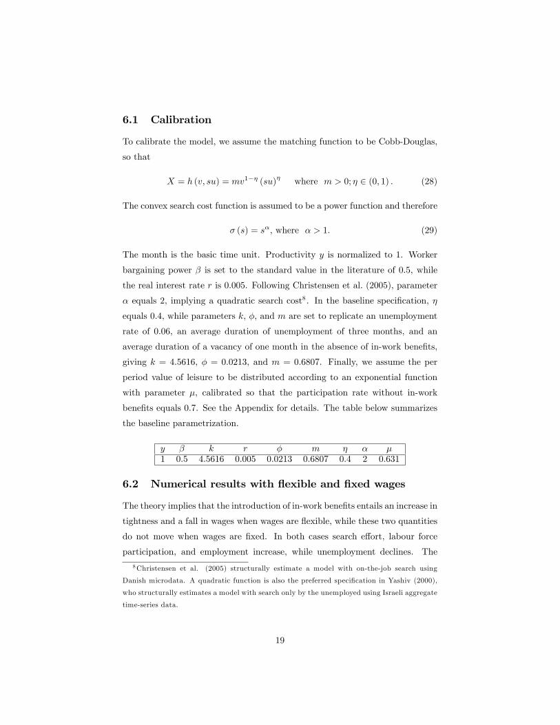
6.1 Calibration
To calibrate the model, we assume the matching function to be Cobb-Douglas,
so that
X = h (v; su) = mv1�� (su)� where m > 0; � 2 (0; 1) . (28)
The convex search cost function is assumed to be a power function and therefore
� (s) = s�, where � > 1. (29)
The month is the basic time unit. Productivity y is normalized to 1. Worker
bargaining power � is set to the standard value in the literature of 0.5, while
the real interest rate r is 0.005. Following Christensen et al. (2005), parameter
� equals 2, implying a quadratic search cost8 . In the baseline speci�cation, �
equals 0.4, while parameters k; �; and m are set to replicate an unemployment
rate of 0:06, an average duration of unemployment of three months, and an
average duration of a vacancy of one month in the absence of in-work bene�ts,
giving k = 4:5616, � = 0:0213, and m = 0:6807. Finally, we assume the per
period value of leisure to be distributed according to an exponential function
with parameter �, calibrated so that the participation rate without in-work
bene�ts equals 0:7. See the Appendix for details. The table below summarizes
the baseline parametrization.
y � k r � m � � �1 0.5 4:5616 0.005 0:0213 0:6807 0.4 2 0.631
6.2 Numerical results with �exible and �xed wages
The theory implies that the introduction of in-work bene�ts entails an increase in
tightness and a fall in wages when wages are �exible, while these two quantities
do not move when wages are �xed. In both cases search e¤ort, labour force
participation, and employment increase, while unemployment declines. The
8Christensen et al. (2005) structurally estimate a model with on-the-job search using
Danish microdata. A quadratic function is also the preferred speci�cation in Yashiv (2000),
who structurally estimates a model with search only by the unemployed using Israeli aggregate
time-series data.
19
conditions under which the impact is greater with or without wage adjustment
have been derived in proposition 2. Here, we explore the quantitative impact of
bene�ts in both cases.
The simulation results show that the quantitative impact on unemployment
and employment is signi�cantly stronger when the e¤ect of bene�ts on wages is
taken into account. Figure 1 describes the e¤ects on the main labour market
variables of introducing in-work bene�ts up to the equivalent of half of labour
productivity. The continuous line represents the case where wages are �exible,
while the dotted line represents the case with �xed wages. Compared to an
unemployment rate of 6% without in-work bene�ts, the introduction of bene�ts
equivalent to 40% of productivity implies a decline in unemployment to 4.97%
when wages are �xed and to 4.41% when they are �exible, while employment
increases by an additional 0.62% with �exible wages as compared to the case
with �xed ones. Moreover, the impact on search intensity and labour force
participation is stronger when wages are allowed to move but quantitatively, the
di¤erence is very small. The fall in wages makes employment less attractive and
so partly, but not entirely, o¤sets the increase in search e¤ort and participation
due to the increase in labour market tightness.
Thus, accounting for the equilibrium impact of bene�ts actually reinforces
their positive e¤ect on the labour market. Thus, the extension of bene�ts to
larger portions of the workforce does not entail, in itself, a decline in their
e¤ectiveness or, worse, a reversal of their e¤ect. In the next section we look
at another issue that needs to be taken into account when the scope of bene�t
programmes is increased to comprise a non negligible share of the workforce:
their �nancing.
6.3 Numerical results with �nancing
Here we use the same parametrization, with the only di¤erence that when sim-
ulating the model with partial �nancing, we also consider the case where the
productivity of non-eligible workers is double the productivity of eligible ones.
First, we compare the e¤ects on the main labour market variables of intro-
20
ducing fully-�nanced bene�ts up to the equivalent of half of labour productivity9
when wages can adjust and when they are instead �xed. We also compare the
impact of bene�ts when their �nancing is accounted for to the impact when the
issue of �nancing is disregarded.
In Figure 2, the continuous line represents the case when wages can adjust,
while the dotted line represents the case with �xed wages. As previously stated,
when bene�ts are fully �nanced by taxing bene�ciaries and wages are downward
rigid, in-work bene�ts do not have any e¤ect. When wages can adjust, tightness
increases and gross wage decreases. Notice that in this setting, gross wage is
equivalent to total income, as �scal revenues are entirely used to �nance bene�ts.
The comparison of �gures 1 and 2 reveals that both tightness and wages respond
more strongly when bene�ts are �nanced through taxation on bene�ciaries�
wages as compared to the case when an identical amount of in-work bene�ts
is a "windfall", �nanced through other sources. This is due to the additional
wage moderation stemming from taxation. As predicted by the theory, with
full �nancing the response of search intensity and labour force participation is
hump-shaped, initially increasing with the level of bene�ts (and taxes) and then
declining. In the baseline parametrization, the tax rate at which both quantities
reach their peak is, from (26), t = 1=3, corresponding to IWB � 0:28, at which(constrained) e¢ ciency is achieved. Further increases in fully �nanced bene�ts
take the labour market away from e¢ ciency. However, search intensity and
participation stay above the level they have when no bene�ts are paid until
IWB � 0:47 (t � 56%). Unemployment declines in the whole range, falling, forinstance, from 6% to 4.15% when bene�ts are equivalent to 40% of productivity.
Total employment increases, reaching approximately 67.2% of the population
when IWB = 0:4, as compared to 65.8% with no bene�ts.
We look at three scenarios in the "partial �nancing" case, where the share
of the population eligible for bene�ts �nanced by the whole workforce is 25%,
50%, and 75%, respectively. To make the comparison easier, we focus on the
case when both eligible and non-eligible workers have the same productivity.
9The tax rate corresponding to IWB = 0:5 is approximately 60%. In the baseline parame-
trization, the maximum attainable amount of bene�ts with wage �exibility is 0.64, achieved
at a tax rate of 88%.
21

However, the case with non-eligible workers having higher productivity is also
investigated.
Figure 3 reports the main labour market indicators for eligible workers as a
function of in-work bene�ts in the three scenarios. For comparison, indicators
with "no �nancing" and "full �nancing" are also depicted. As could be expected,
the "partial �nancing" cases lie between the two polar ones, moving toward the
"full �nancing" equilibrium as the share of eligible workers increases. The cor-
responding �gure for non-eligible workers is 4. For this group of workers, given
the share of eligibles in the population, an increase in bene�ts just represents an
increase in taxation. An increase in the share of eligible workers, given a level
of bene�ts, also represents an increase in taxation. Thus, increasing bene�ts or
increasing eligibility reduce wages, search intensity, labour force participation,
and employment of non-eligible workers, while tightness and unemployment in-
crease.
The impact of bene�ts on the labour market as a whole is presented in
�gure 5, that includes the "full �nancing" case for reference, and in table 1.
Unemployment decreases with the introduction of bene�ts, and the impact on
it is stronger as bene�ts increase and as the share of eligible workers increases,
with the equilibrium smoothly converging to the "full �nancing" case. The
behavior of labour force participation and employment is more complex. Their
response to bene�ts is hump-shaped, �rst increasing and then decreasing as
bene�ts increase. The response to an increase in eligibility is also non-linear.
For a given level of bene�ts, labour force participation and employment may
decrease with the share of the population eligible for bene�ts rising from 25%
to 50%, but then bounce back with a further increase to 75%. While improving
labour market conditions for eligible workers, the negative impact of increased
taxation on non-eligible ones implies that in-work bene�ts above a relatively
low level do not improve participation and employment in the labour market
as a whole. This no longer happens if the productivity of non-eligible workers
is set to double the productivity of eligible ones (see table 2). In this case,
labour market conditions improve with the introduction of bene�ts even at
relatively high levels. The analysis of the partial �nancing case done here is
just preliminary, but indicates the importance of accounting for the �nancing
22

of bene�ts when evaluating their impact on the labour market as a whole.
7 Conclusions
In-work bene�ts are becoming increasingly popular among policy-makers due
to their success in the American and British contexts. Whether they can be
successfully adopted in other countries and help solve some of the problems
characterizing their labour markets is an open issue. This paper represents a �rst
step towards addressing this question. We analyze the impact of in-work bene�ts
on some of the main labour market indicators in a search framework, taking into
account the e¤ects on labour market equilibrium . We �nd that introducing or
increasing in-work bene�ts increases labour force participation, employment,
and search intensity by unemployed, while wages and the unemployment rate
decline. This result is robust to various extensions.
Considering in-work bene�ts in an equilibrium setting reveals that their im-
pact on job creation is an important factor behind employment growth, in con-
trast to the existing literature that mainly looks at their impact on labour supply
via a higher take-home pay. In fact, in-work bene�ts may even reduce the take-
home pay as wage demands are moderated10 . However, the lower wages boost
job creation which reduces unemployment. The shorter expected unemploy-
ment spell, in turn, encourages job search and labour force participation which
reinforces the increase in employment. Our model suggests that the job cre-
ation dimension should be taken into account in evaluating ex ante the impact
of introducing such bene�ts in a European country. The risk is, otherwise, to
miss a very important link.
The analysis of �nancing reveals the conditions under which bene�ts that
are �nanced through proportional taxation on wages increase labour force par-
ticipation, employment, and search intensity of the targeted group.
Both these aspects of in-work bene�ts, their impact on job creation and their
�nancing, have mostly been overlooked by the existing literature, but become
increasingly relevant as the scope of programmes including bene�ts or tax credits
10This was concluded in section 4, where unemployment bene�ts were indexed to the wage
which induced additional wage moderation which could actually reduce the take-home pay.
23

conditioned on labour income is extended.
References
[1] Blundell, R., 2006. Earned income tax policies: impact and optimality.
Journal of Labour Economics 13, 423-443.
[2] Boeter, S., Schnabel, R., and Gurtzgen, N., 2006. Reforming social welfare
in Germany; An applied general equilibrium analysis. German Economic
Review 7, 363-388.
[3] Brewer, M., and Browne, J., 2006. The e¤ect of the working families�tax
credit on labour market participation. BN No 69, the Institute for Fiscal
Studies.
[4] Boone J., and Bovenberg, L., 2004. The optimal taxation of unskilled labour
with job search and social assistance. Journal of Public Economics 88, 2227-
2258.
[5] Boone J., and Bovenberg, L., 2006. Optimal welfare and in-work bene�ts
with search unemployment and observable abilities. Journal of Economic
Theory 126, 165-193.
[6] Christensen, B. J., Lentz, R., Mortensen, D. T., Neumann, G. R., and
Wervatz, A., 2005. On the job search and the wage distribution. Journal of
Labor Economics 23, 31-58.
[7] Eissa, N., and Hoynes, H., 2004. Taxes and the labour market participa-
tion of married couples; The earned income tax credit. Journal of Public
Economics 88, 1931-1958.
[8] Eissa, N., and Hoynes, H., 2005. Behavioral responses to taxes; Lessons
from the EITC and labour supply. forthcoming in Tax Policy and the Econ-
omy.
[9] Eissa, N., and Liebman, J., 1996. Labor supply responses to the earned
income tax credit. Quarterly Journal of Economics 111, 605-637.
24

[10] Fang, H., and Keane, M., 2004. Assessing the Impact of Welfare Reform
on Single Mothers. Brookings Papers on Economic Activity 1, 1-116.
[11] Immervoll, H., Kleven, H., Kreiner, C.T. and Saez, E., 2007. Welfare reform
in European countries: A micro simulation analysis. Economic Journal 117,
1-44.
[12] Leigh, A., 2004. Who Bene�ts from the Earned Income Tax Credit? In-
cidence Among Recipients, Coworkers and Firms, ANU CEPR Discussion
Paper 494.
[13] Lise, J., Shannon, S., and Smith, J., 2005. Equilibrium policy experiments
and the evaluation of social programs. IZA Working Paper 758.
[14] Meyer, B., and Rosenbaum, D., 2001. Welfare, the earned income tax credit
and the labour supply of single mothers. Quarterly Journal of Economics
116, 1063-1114.
[15] Meyer B., 2002. Labor Supply at the Extensive and Intensive Margin, the
EITC, Welfare and Hours Worked. American Economic Review. Papers
and Proceedings 92, 373-379.
[16] Michalopoulos C., Robins, P.K., and Card, D., 2005. When Financial Work
Incentives Pay for Themselves; Evidence from a Randomized Social Exper-
iment for Welfare Recipients. Journal of Public Economics 89, 5-29.
[17] Pissarides, C., 2000. Equilibrium unemployment theory, MIT Press,
Boston, MA.
[18] Rothstein, J., 2004. The Unintended Consequences of Encouraging Work:
Is the EITC As Good As an NIT?, mimeo.
[19] Saez, E., 2002. Optimal Income Transfer Programs: Intensive Versus Ex-
tensive Labor Supply Responses. Quarterly Journal of Economics 117,
1039-1073.
[20] Yashiv, E., 2000. The determinants of equilibrium unemployment. The
American Economic Review 90, 1297-1322.
25

Appendix
A1 Proofs of propositions
Proposition 1. Di¤erentiation of (10) with respect to � and IWB yields
@�@IWB =
(1��)s�k
�1�k(r+�) q0
s�kq2
� > 0: To get the equilibrium e¤ect on tightness, we
need to account for the fact that s is a function of � through (11). However, as
search is optimally determined by workers, the e¤ects working through search
e¤ort in (10) will have no impact on tightness. Using how IWB a¤ects tight-
ness and the fact that search is optimally determined, we can show the following
for search e¤ort, wage, income from work, labour force participation, the un-
employment rate, and employment: @s@IWB = �k
�ss(s)(1��)@�
@IWB > 0 from (11),@w
@IWB = � (1� �)h1� 1=
�1� k (r + �) q0
s�kq2
�i< 0 from (8), @(w+IWB)
@IWB =
� (1� �)h1� 1=
�1� k (r + �) q0
s�kq2
�i+1 > 0, @LF
@IWB = F0 (:) s�k
(1��)@�
@IWB � 0from (12), @u
@IWB = � ��+s(�)�(�)
�@s@�� (�) + s
@�@�
�@�
@IWB < 0 from (13), and@Employment
@IWB = � @u@IWBLF + (1� u)
@LF@IWB > 0 from (14).
Proposition 2. Optimal search is determined by (15). Di¤erentiation of
(15) gives: @s@IWB = �(�)
N + AN where N = �ss (s) (r + �+ s� (�)) and A =
� (�) @w@IWB +
@�(�)@�
1�(�)
@�@IWB�s (:) (r + �). The �rst term captures the direct
e¤ect (and only e¤ect if wages are �xed) and the second term captures the ef-
fects due to �exible wages. As the �rst term is the same in the �xed and �exible
case, the e¤ect on search due to wage adjustments depends on the sign of the
second term. Using the expressions in the proof of proposition 1 and the fact
that � (�) = q� and @�(�)@� = q0� + q, we have A = (r+�)
(s�+(r+�)�(�)=�(�)) [� � �] >0$ � > �. Use (15) to rewrite (16) as LF = F (s�s (s)� � (s)) :Di¤erentiationyields @LF
@IWB = F 0 (:) s�ss (s)@s
@IWB . Therefore, the condition for labour force
participation to increase more with a marginal increase in IWB under �ex-
ible wages is the same as the one for search intensity. Moreover, @u@IWB =
� ��+s(�)�(�)
�@s
@IWB� (�) + s@�(�)@�
@�@IWB
�: Thus the unemployment rate tends
to fall by more when wages are �exible as the higher tightness increases the
transition rate into employment irrespective of whether � is larger or smaller
than �. However, if � > � (�), search increases by more if wages are �exi-
26

ble, and thus we have an additional negative e¤ect on the unemployment rate,
making � > � (�) a su¢ cient but not necessary condition for unemployment to
decline more when wages are �exible. This is also the case for employment, as@Employment
@IWB = � @u@IWB + (1� u)
@LF@IWB .
A2 Expressions and calibration
The expressions we used in the calibration are derived in this appendix.
No �nancing Using (29) in (11), we get
s =
��k�
� (1� �)
� 1��1
; (30)
that, substituted into (10) and together with (28), gives
k (r + �)
m���= (y + IWB) (1� �)�
�1� 1
�
�(�k�)
���1
[� (1� �)]1
��1; (31)
which implicitly determines equilibrium tightness as a function of parameters.
Equilibrium search is given by substituting equilibrium tightness into (30).
Given that � and s are determined by (30) and (31), we can derive the wage,
the unemployment rate, the labour force and employment in the following way.
>From (8) we get the equilibrium wage
w = � (y + ks�)� (1� �) [IWB + s�] ;
and from (13) the equilibrium unemployment rate
u =�
�+ sm�1��: (32)
>From (12) and the assumption that the per period value of leisure is distributed
according to an exponential function with parameter �, we get the labour force
LF = 1� exp � (�� 1)
�
��k�
� (1� �)
� ���1!; (33)
and, �nally, from (14) we can derive the equilibrium employment.
27

With �nancing Using (29) in (22), we get
s =
�(1� t)�k�� (1� �)
� 1��1
; (34)
which, substituted into (21) and together with (28), gives
k (r + �)
m���=1� �1� �t
"y + (1� �)
�(1� t)�k�� (1� �)
� ���1#; (35)
that implicitly determines equilibrium tightness as a function of parameters.
Equilibrium search is given by substituting equilibrium tightness into (34).
Given that � and s are determined by (34) and (35), we can derive the wage,
the unemployment rate, the labour force and employment in the following way.
From (20), we get the equilibrium wage
w = � [y + ks� + s�]1� t1� �t � s
�;
and from (19), the corresponding in-work bene�ts, IWB. Labour force partic-
ipation is given by (24)
LF = 1� exp�� (�� 1)
�
�(1� t)�k�� (1� �)
��;
while the expressions for unemployment and unemployment are the same as in
the case without �nancing.
Partial Financing For non-eligible workers, tightness is given by
k (r + �)
m���n= (1� �) yn � (�� 1)
1� �1� t
�(1� t)�k�n� (1� �)
� ���1
;
and the wage is given by
wn = � (yn + ksn�n)�1� �1� t s
�n;
while the other expressions are the same as in the total �nancing case.
For eligible workers, tightness is given by
k (r + �)
m���e
�1� �t1� �
�=
0BB@ye + b
�
1 + �h(1�t)�k�e�(1��)
i� 1��1
m�1���1e
1� exp����1
�
h(1�t)�k�e�(1��)
i ���1�1CCA+(1� �) � (1� t)�k�e� (1� �)
� ���1
:
28

The wage is given by
we =� (1� t)1� �t (ye + kse�e)�
1� �1� �t
�b
�ee+ s�e
�;
while the other expressions are the same as in the total �nancing case. The
labour force participation rate for the economy as a whole is given by
LF = �LFe + (1� �)LFn;
while total employment is given by
E = �ee + (1� �) en:
The unemployment rate for the economy as a whole is
u =�LFeue + (1� �)LFnun
LF;
and the average wage is
w =�eewe + (1� �) enwn
E:
Fixed wages Expression (15) becomes
m�1��(�� 1)s� + �s��1 (r + �)�m�1�� ( ~w + IWB) = 0;
while expression (16) is given by
LF = 1� exp�� 1�sm�1��
~w + IWB + s�
r + �+ sm�1��+1
�s��:
Calibration Parameters k; �;m are set to replicate an unemployment rate of
�u, an average duration of unemployment of du months, and an average duration
of a vacancy of dv months in the absence of in-work bene�ts. Unemployment is
given by (32), so that�
�+ sm�1��= �u:
Expected duration of unemployment is given by
1
s� (�)=
1
sm�1��= du:
29

Expected duration of a vacancy is given by
1
q (�)=
1
m���= dv:
Substituting the value of the expected duration of unemployment in the expres-
sion for unemployment, we pin down the value of �:
�u =�
�+ 1du
() � =�u
du (1� �u):
Taking the ratio of the expected duration of unemployment and of a vacancy
we havedvdu= s�:
Substituting from (30) we get
dvdu=
��k
� (1� �)
� 1��1
��
��1 () � =
�dvdu
���1��� (1� �)�k
� 1�
:
Taking (31) with IWB = 0 and substituting we get
� =� (1� �)
1�
�k
�y (1� �)� k (r + �) dv
�� 1
���1�
:
The two expressions together imply
k =(1� �)�
1� 1�
���dvdu
�+ (r + �) dv
y:
The corresponding tightness is given by substituting k into one of the two above
expressions, i.e.
� =
�dvdu
���1�
24 (�� 1)��dvdu
�+ � (r + �) dv
�y
351�
;
while m, the matching function scale parameter, is given by
1
m���= dv () m =
��
dv;
and s, search intensity, by
s =dv�du
:
The chosen parameter values plus the calibration of an unemployment rate of
0:06, an average duration of unemployment of three months, and an average
30

duration of a vacancy of one month in the case without in-work bene�ts imply
a separation rate � = 0:0213 (equivalent to an annual separation rate of 0:255),
a vacancy cost k = 4:5616, with the corresponding tightness � = 0:3823, the
scale parameter of the matching function m = 0:6807, while search is given by
s = 0:8719. Using (33), we get the distribution parameter as
� s:t: F
�s�k�
(1� �) � s�;�
�= �L
which, in case of an exponential distribution, is equivalent to
� =1
ln�1� �L
� � s�k�
(1� �) � s�
�and gives a value of � = 0:631 for a labour force participation without in-work
bene�ts equal to 0:7.
31
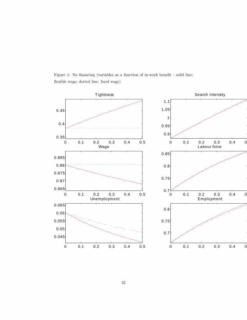
Figure 1: No �nancing (variables as a function of in-work bene�t - solid line:
�exible wage; dotted line: �xed wage)
0 0.1 0.2 0.3 0.4 0.50.35
0.4
0.45
T ightness
0 0.1 0.2 0.3 0.4 0.5
0.9
0.95
1
1.05
1.1
Search intensi ty
0 0.1 0.2 0.3 0.4 0.50.865
0.87
0.875
0.88
0.885
Wage
0 0.1 0.2 0.3 0.4 0.50.7
0.75
0.8
0.85
Labour force
0 0.1 0.2 0.3 0.4 0.5
0.045
0.05
0.055
0.06
0.065Unemployment
0 0.1 0.2 0.3 0.4 0.5
0.7
0.75
0.8
Employment
32
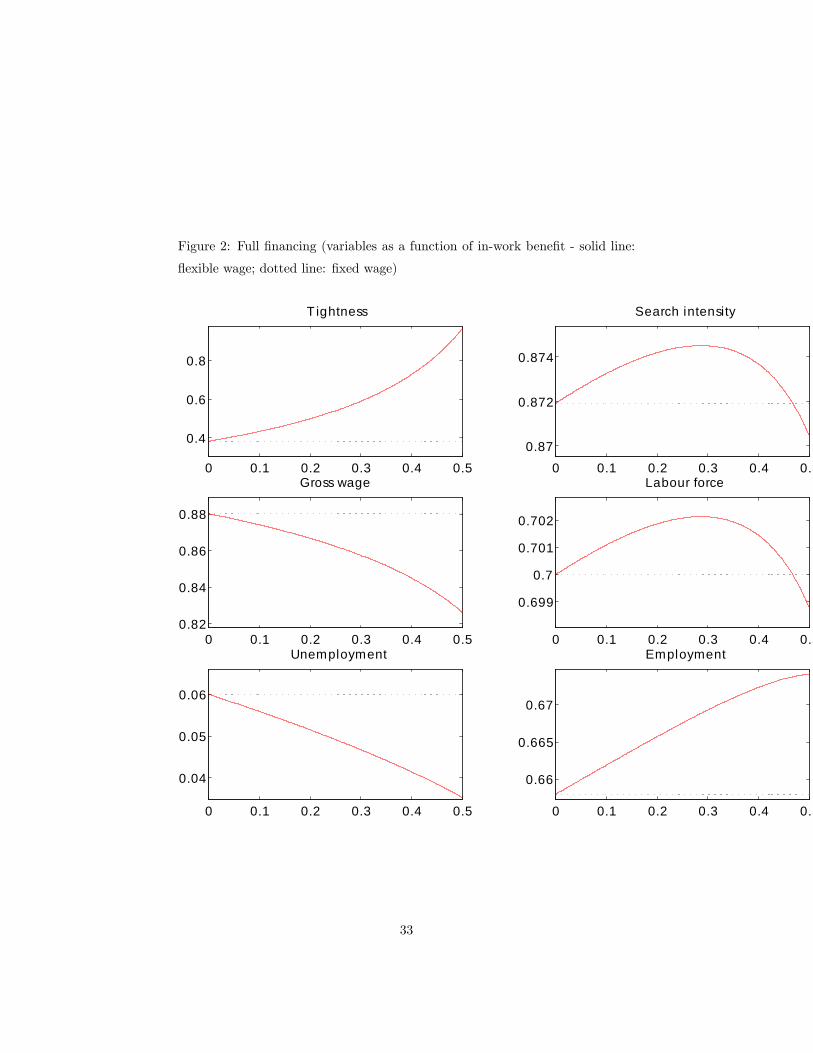
Figure 2: Full �nancing (variables as a function of in-work bene�t - solid line:
�exible wage; dotted line: �xed wage)
0 0.1 0.2 0.3 0.4 0.5
0.4
0.6
0.8
T ightness
0 0.1 0.2 0.3 0.4 0.50.87
0.872
0.874
Search intensity
0 0.1 0.2 0.3 0.4 0.50.82
0.84
0.86
0.88
Gross wage
0 0.1 0.2 0.3 0.4 0.5
0.699
0.7
0.701
0.702
Labour force
0 0.1 0.2 0.3 0.4 0.5
0.04
0.05
0.06
Unemployment
0 0.1 0.2 0.3 0.4 0.5
0.66
0.665
0.67
Employment
33
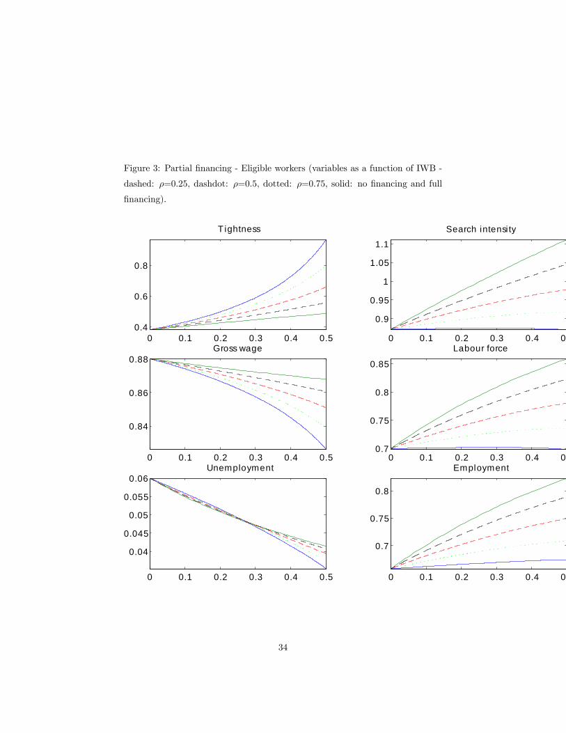
Figure 3: Partial �nancing - Eligible workers (variables as a function of IWB -
dashed: �=0.25, dashdot: �=0.5, dotted: �=0.75, solid: no �nancing and full
�nancing).
0 0.1 0.2 0.3 0.4 0.50.4
0.6
0.8
T ightness
0 0.1 0.2 0.3 0.4 0.5
0.9
0.95
1
1.05
1.1
Search intensi ty
0 0.1 0.2 0.3 0.4 0.5
0.84
0.86
0.88Gross wage
0 0.1 0.2 0.3 0.4 0.50.7
0.75
0.8
0.85
Labour force
0 0.1 0.2 0.3 0.4 0.5
0.04
0.045
0.05
0.055
0.06Unemployment
0 0.1 0.2 0.3 0.4 0.5
0.7
0.75
0.8
Employment
34
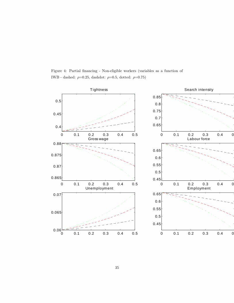
Figure 4: Partial �nancing - Non-eligible workers (variables as a function of
IWB - dashed: �=0.25, dashdot: �=0.5, dotted: �=0.75)
0 0.1 0.2 0.3 0.4 0.5
0.4
0.45
0.5
T ightness
0 0.1 0.2 0.3 0.4 0.5
0.65
0.7
0.75
0.8
0.85
Search intensi ty
0 0.1 0.2 0.3 0.4 0.5
0.865
0.87
0.875
0.88Gross wage
0 0.1 0.2 0.3 0.4 0.50.45
0.5
0.55
0.6
0.65
Labour force
0 0.1 0.2 0.3 0.4 0.50.06
0.065
0.07
Unemployment
0 0.1 0.2 0.3 0.4 0.5
0.45
0.5
0.55
0.6
0.65Employment
35

Figure 5: Partial �nancing - All workers (variables as a function of IWB -
dashed: �=0.25, dashdot: �=0.5, dotted: �=0.75, solid: full �nancing)
0 0.1 0.2 0.3 0.4 0.5
0.83
0.84
0.85
0.86
0.87
0.88Gross wage
0 0.1 0.2 0.3 0.4 0.5
0.66
0.67
0.68
0.69
0.7
Labour force
0 0.1 0.2 0.3 0.4 0.5
0.04
0.045
0.05
0.055
0.06Unemployment
0 0.1 0.2 0.3 0.4 0.5
0.63
0.64
0.65
0.66
0.67
Employment
36
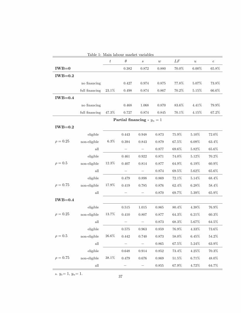
Table 1: Main labour market variables
t � s w LF u e
IWB=0 0.382 0.872 0.880 70.0% 6.00% 65.8%
IWB=0.2
no �nancing 0.427 0.974 0.875 77.8% 5.07% 73.8%
full �nancing 23.1% 0.498 0.874 0.867 70.2% 5.15% 66.6%
IWB=0.4
no �nancing 0.468 1.068 0.870 83.6% 4.41% 79.9%
full �nancing 47.3% 0.727 0.874 0.845 70.1% 4.15% 67.2%
Partial �nancing - yn = 1
IWB=0.2
� = 0:25
eligible
non-eligible
all
6.3%
0.443
0.394
�
0.948
0.843
�
0.873
0.879
0.877
75.9%
67.5%
69.6%
5.10%
6.09%
5.82%
72.0%
63.4%
65.6%
� = 0:5
eligible
non-eligible
all
12.3%
0.461
0.407
�
0.922
0.814
�
0.871
0.877
0.874
74.0%
64.9%
69.5%
5.12%
6.19%
5.62%
70.2%
60.9%
65.6%
� = 0:75
eligible
non-eligible
all
17.9%
0.479
0.419
�
0.898
0.785
�
0.869
0.876
0.870
72.1%
62.4%
69.7%
5.14%
6.28%
5.39%
68.4%
58.4%
65.9%
IWB=0.4
� = 0:25
eligible
non-eligible
all
13.7%
0.515
0.410
�
1.015
0.807
�
0.865
0.877
0.873
80.4%
64.3%
68.3%
4.38%
6.21%
5.67%
76.9%
60.3%
64.5%
� = 0:5
eligible
non-eligible
all
26.6%
0.575
0.442
�
0.963
0.740
�
0.859
0.873
0.865
76.9%
58.0%
67.5%
4.33%
6.45%
5.24%
73.6%
54.2%
63.9%
� = 0:75
eligible
non-eligible
all
38.1%
0.648
0.479
�
0.914
0.676
�
0.852
0.869
0.855
73.4%
51.5%
67.9%
4.25%
6.71%
4.72%
70.3%
48.0%
64.7%
a. ye= 1; yn= 1: 37
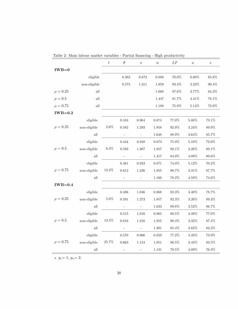
Table 2: Main labour market variables - Partial �nancing - High productivity
t � s w LF u e
IWB=0
eligible 0.382 0.872 0.880 70.0% 6.00% 65.8%
non-eligible 0.575 1.311 1.859 93.4% 3.22% 90.4%
� = 0:25 all 1.668 87.6% 3.77% 84.3%
� = 0:5 all 1.447 81.7% 4.41% 78.1%
� = 0:75 all 1.188 75.9% 5.14% 72.0%
IWB=0.2
� = 0:25
eligible
non-eligible
all
2.6%
0.434
0.582
-
0.964
1.293
-
0.874
1.858
1.648
77.0%
92.9%
88.9%
5.08%
3.24%
3.64%
73.1%
89.9%
85.7%
� = 0:5
eligible
non-eligible
all
6.3%
0.444
0.593
-
0.948
1.267
-
0.873
1.857
1.417
75.9%
92.1%
84.0%
5.10%
3.26%
4.09%
72.0%
89.1%
80.6%
� = 0:75
eligible
non-eligible
all
12.2%
0.461
0.612
-
0.923
1.226
-
0.871
1.855
1.160
74.0%
90.7%
78.2%
5.12%
3.31%
4.59%
70.2%
87.7%
74.6%
IWB=0.4
� = 0:25
eligible
non-eligible
all
5.6%
0.486
0.591
-
1.046
1.273
-
0.868
1.857
1.633
82.3%
92.3%
89.8%
4.40%
3.26%
3.52%
78.7%
89.3%
86.7%
� = 0:5
eligible
non-eligible
all
13.5%
0.515
0.616
-
1.016
1.216
-
0.865
1.855
1.391
80.5%
90.4%
85.4%
4.38%
3.32%
3.82%
77.0%
87.4%
82.2%
� = 0:75
eligible
non-eligible
all
25.7%
0.570
0.663
-
0.966
1.124
-
0.859
1.851
1.131
77.2%
86.5%
79.5%
4.33%
3.43%
4.09%
73.9%
83.5%
76.3%
a. ye= 1; yn= 2:
38