Ination and unemployment in the open economyuctpa36/ch5feb0303.pdf · Ination and unemployment in the open economy ... What factors inuence the rate of unemployment and output level

CHAPTER 5

In�ation and unemployment in theopen economy

[This is a draft chapter of a new book - Carlin & Soskice (200x)1].This chapter brings together the supply side of the economy with the demand side and the trade

balance to provideabasic model for analyzing theopen economy. It buildson the imperfect compe-tition model of the supply side developed in Chapters 1 to 3 and on the Mundell–Fleming short-runmodel of the open economy developed in Chapter 4. The basic model can be used to answer thefollowing questions:

� What determines the level of output and employment in theshort run?� What factors in�uence the rate of unemployment and output level that can be sustained in

themedium run without problems of in�ation?� Why might a medium-run position of stable in�ation but trade imbalance be unsustainable

in the long run?

In this chapter, we explore a key difference between an open and a closed economy. In an openeconomy, thereisarangeof unemployment ratesconsistent with theabsenceof in�ationary pressure.By contrast, in the closed economy, there is a unique unemployment rate consistent with constantin�ation. The reason for this difference lies with the impact of changes in the real exchange rate onthesupply sideof theeconomy.

In the open economy it will generally be the case that the wage-setting real wage and the price-setting real wage are equal over a range of unemployment rates: this is what is required to delivera range of constant in�ation equilibrium unemployment rates. The wage-setting curve is just thesameas in theclosed economy: asemployment rises, thewage-setting real wagerises. In theclosedeconomy, the price-setting real wage is constant (or downward sloping). Hence there is just onelevel of employment at which the wage and price-setting real wages are equal: this fixes the uniqueequilibrium rate of unemployment (��), or �� , as it is often called in empirical studies.But in the open economy, the price setting real wage is a function of the real exchange rate: it willshift up and down as the real exchange rate changes. The simplest way to think of this is that whenthereal exchangeratedepreciates, thereal cost of importsgoesup and this reduces theprice-settingreal wage. The�exibility of the real exchange rate and hence of the real cost of imports means thattheprice-setting real wagecan beequal to thewage-setting real wageover arangeof unemploymentrates. It is intuitively plausible that as the economy moves closer to being closed, the range ofequilibrium unemployment rates narrows: in theclosed economy there is aunique�� .

Sincethere isarangeof constant in�ation unemployment rates in theopen economy, can macro-economic policy makers choose any desired unemployment rate by using fiscal policy to alter thelevel of aggregate demand? Policy makers in the open economy are likely to be constrained by theconsequences of their actions for the external balance. If the economy is running either a persistentcurrent account surplusor deficit, thereareanumber of mechanismsthat arelikely to comeinto playat somestage that push theeconomy toward current account balance. Thesepressures arisebecausethe surplus or deficit represents a change in theeconomy’s wealth position. A change in wealth canaffect private sector expenditure and access to international capital markets. Equally, a persistentdeficit or surplus may affect exchange rate expectations. In the long run it is likely that the currentaccount position will placeaconstraint on theunemployment rate.

1 c�Wendy Carlin & David Soskice (2003). Wearevery grateful to Andrew Glyn, Georg von Graevenitz, CameronHepburn, Massimo di Matteo, Nicholas Rau and William Wachtmeister for their help and advicebut weareresponsiblefor all errors.

1

2 5. INFLATION AND UNEMPLOYMENT IN THE OPEN ECONOMY

This chapter begins by asking how wages and prices react in the open economy following themove to a new short run equilibrium. We then integrate the supply side more systematically intoopen economy analysis. A new core diagram that is used from this point onwards in the book isintroduced. The diagram has the real exchange rate and output on the axes. Section 3 is short— it simply shows how to translate the demand side and trade balance analysis from Chapter 4into the new diagram. In the third section, the demand and supply sides are put together to createthe basic open economy model. The differences between the short-run, medium-run (i.e. constantin�ation) and long-run (i.e. current account balance) equilibriaareexamined. Thechapter concludeswith a discussion of the reasons why in the longer run, the economy may be constrained to anunemployment rateclose to current account balance.

1. In�ation and unemployment in theopen economy

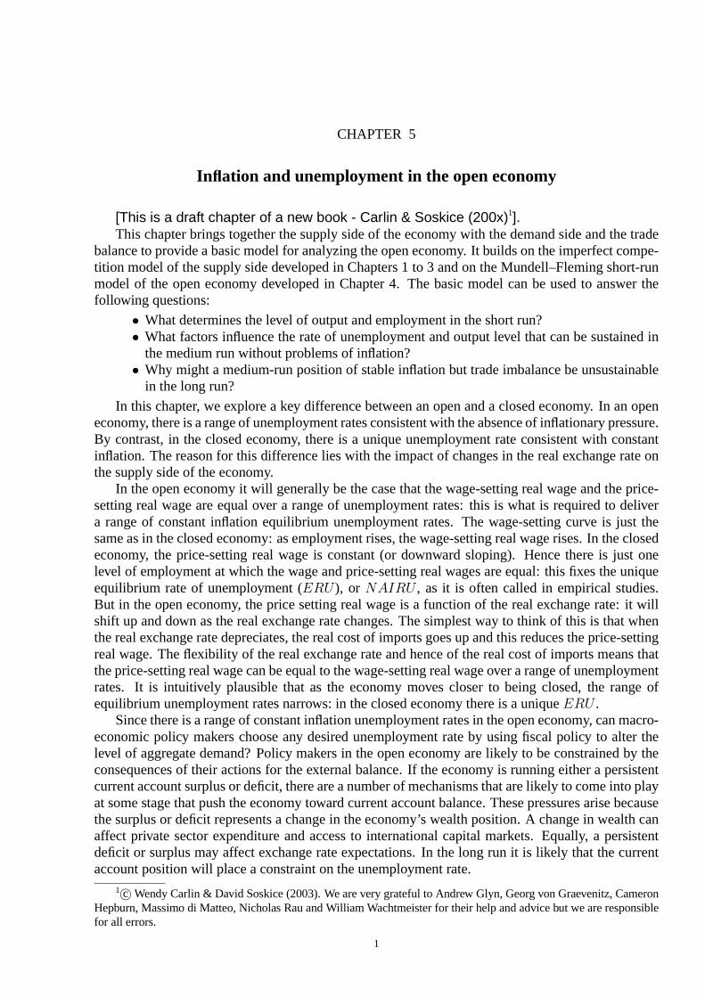
In what ways do we need to alter the analysis of the supply side in the closed economy to makeit fit the open economy? First, let us recall the closed economy model. Medium run equilibriumin the closed economy is characterized by constant in�ation: the rate of unemployment at whichin�ation is constant is referred to as the ‘equilibrium’ rate, the�� (or ��). For illustrativepurposes it is simplest to assume constant labour productivity, �� , and a constant mark-up. Giventhewage-setting curveand theprice-setting curve, thereisasingleemployment level (and associatedunemployment rate) at which the expected real wage set by wage-setters is equal to the real wagethat is implied by price-setting behaviour. Equilibrium employment, ��, is shown in Fig. 5.1.

��

��

��

��

��

��

�

��

��

��

FIGURE 1. Equilibr ium employment in theclosed economy

At �� for a given expected in�ation rate, money wages will rise in line with expected in�ationto deliver the real wage � and prices will rise in line with money wages to keep the profit marginunchanged. Thus in�ation will remain equal to itsexpected rate: there isconstant in�ation at ��. Atany other employment level, the wage-setting real wage will be either higher than the price-settingreal wage (when employment is higher than ��) or lower than the price-setting real wage (whenemployment is lower than ��). There will be upward pressure on in�ation in the first case anddownward pressure in the second case. In�ation will be constant only when employment is at ��because only here are the expectations of both wage and price-setters fulfilled. There is no pressureon in�ation. This is the medium-run equilibrium. In a�exible exchange rate economy in a mediumrun equilibrium, in�ation will be constant at the growth rate of the money supply set by the centralbank or at thecentral bank’s in�ation target if it isusing amonetary policy rulesuch asaTaylor rule.In a fixed exchange rate economy, in�ation will be constant at the growth rate of the money supply

1. INFLATION AND UNEMPLOYMENT IN THE OPEN ECONOMY 3

set by the central bank in the large economy to which its exchange rate is pegged or at that centralbank’s in�ation target.

Inan openeconomy with imperfect competition, thedemand for thegoodsandservicesproducedby homefirmswill depend on the level of demand in thehomeeconomy and in theworld and on therelative price and non-price characteristics of the product. Similarly, the demand by home residentsfor goods and services produced abroad will depend on the level of demand in the home economyandon thepriceandnon-priceattributesof theforeigngoodsandservices. Thesefactorsarere�ectedin the export and import functions (Chapter 4), where we saw how aggregate demand and the tradebalance are affected by changes in the real exchange rate. But what is the significance of opennessfor thesupply sideof theeconomy?

One way to get a feel for this is to work through some examples, beginning with familiar sit-uations that we have considered in Chapter 4. We shall begin with the economy in a medium-runequilibrium with constant in�ation and then implement a change in fiscal or monetary policy. Afternoting thenew short-run equilibrium, weask how pricesand wageswill moveoncethey areallowedto adjust. We shall see that wages and prices not only react to changes in the level of output (as inthe closed economy) following changes to fiscal or monetary policy but also to any change in thereal exchange rate that has occurred. This is because a change in the real exchange rate affects realwages and thereforedisturbs theequilibrium in the labour market.

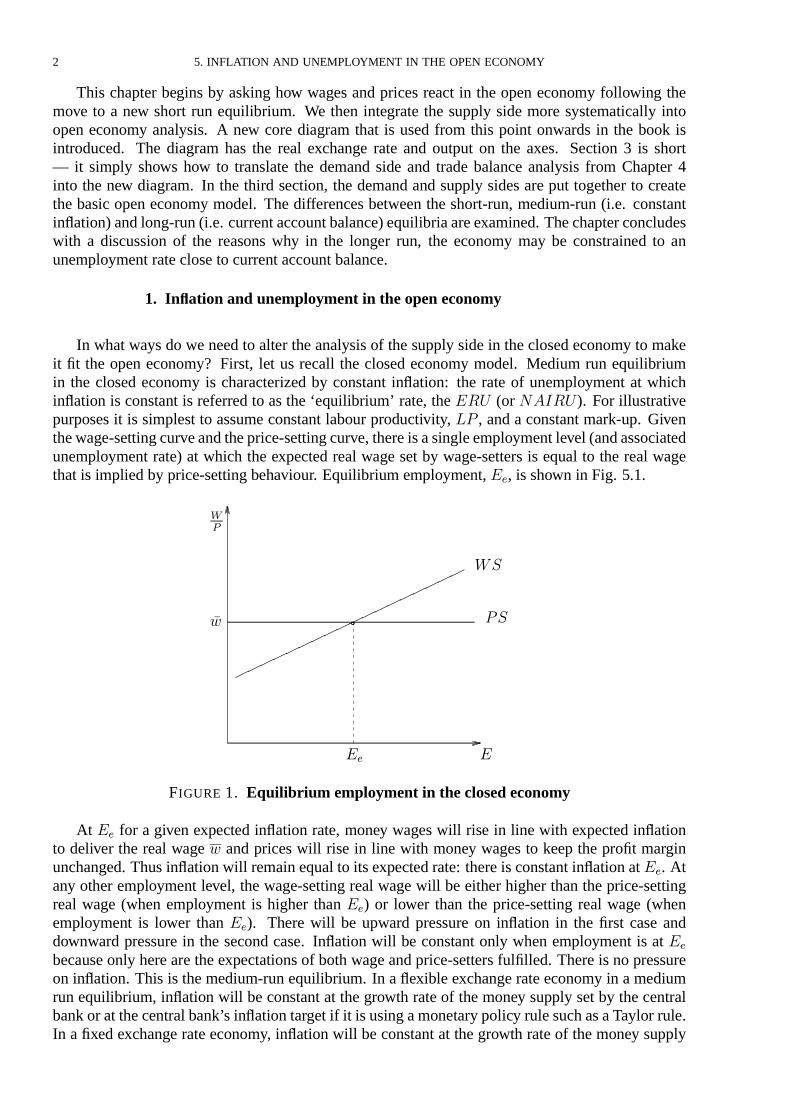
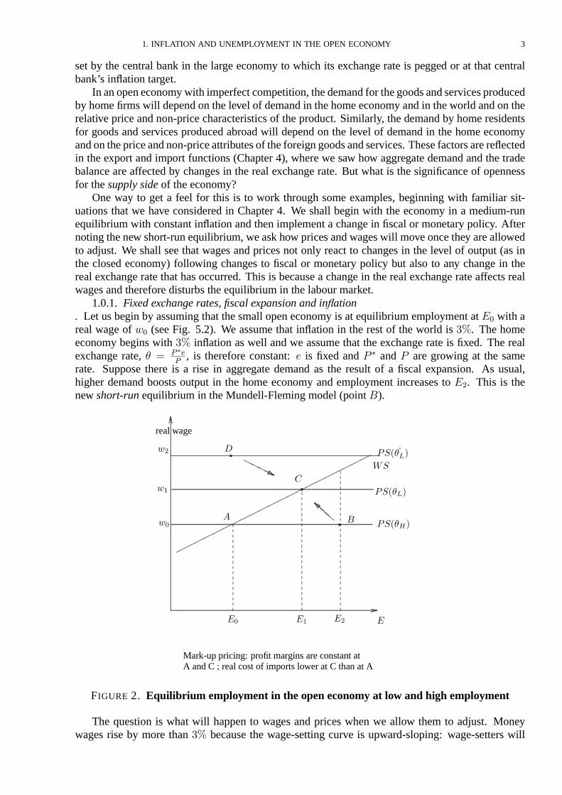
1.0.1. Fixed exchange rates, fiscal expansion and in�ation. Let us begin by assuming that thesmall open economy is at equilibrium employment at �� with areal wage of �� (see Fig. 5.2). We assume that in�ation in the rest of the world is ��. The homeeconomy begins with �� in�ation as well and we assume that the exchange rate is fixed. The realexchange rate, � � ��

�, is therefore constant: is fixed and � � and � are growing at the same

rate. Suppose there is a rise in aggregate demand as the result of a fiscal expansion. As usual,higher demand boosts output in the home economy and employment increases to ��. This is thenew short-run equilibrium in theMundell-Fleming model (point �).

��

��

��

��

��

��

��

�

��

��

�

��

�

real wage

��

��

��

��

��

Mark-up pricing: profit marginsareconstant at

�

��

A and C � real cost of imports lower at C than at A

��

�

�

��

FIGURE 2. Equilibr ium employment in the open economy at low and high employment

The question is what will happen to wages and prices when we allow them to adjust. Moneywages rise by more than �� because the wage-setting curve is upward-sloping: wage-setters will


require a higher expected real wage. The unit costs of home firms therefore increase. According toour usual assumption about pricing behaviour, home firms raise their prices to re�ect these highercosts(so homepriceswill rise in linewith wages, i.e. at arateabove��). This in turn pushesup theconsumer price index. This is an open economy so home consumers buy both imported goods andhome produced goods. Since the price of imported goods has only risen by ��, the consumer priceindex does not rise by as much as does the price index of home produced goods. This has a veryimportant consequence. The rise in consumer priceswipes out somebut not all of the rise in moneywages: hence the real wage increases.

But there is something else going on as well: as home prices are pushed up relative to worldprices, the home economy loses competitiveness (the real exchange rate appreciates) and outputand employment fall below ��. The economy moves north-west from � as shown by the arrow.Will employment shrink right back to its initial level of ��? To find out the answer, rememberthat government spending is higher (due to the expansionary fiscal policy). That means that for theeconomy to return to point � so there is no change in output, the real exchange rate would have toappreciate in order to reduce net exports by the full amount of the increase in government spending(i.e. �� ). But if thereal exchangerateat point � hasappreciated relativeto its initiallevel, then the real cost of imports will be lower (since�� , which has fallen) andreal wages will therefore be higher than they were initially. If so, the labour market will not be inequilibrium since the real wage will be above the wage-setting real wage (i.e. � � �� at��).

This implies that when we allow prices and wages to adjust following a fiscal expansion underfixed exchange rates, the economy will end up in a medium-run equilibrium at a point such as�: with employment higher than initially and with in�ation constant. Since home producers haveprotected their profit margins throughout, thewage-setting real wageand theprice-setting real wageare equal at the new higher level of employment. We have therefore found a second equilibriumemployment level at ��.

Thesequenceof events is summarized as follows:

�� new short-run equilibrium isestablished (�) � � �� and��

�� wages& pricesadjust to change in� : � � �� relative to � �� and � ��

� new medium-run equilibrium isestablished (�) � constant, � higher, � lower, � higher

If real wages arehigher and real profitsare the same, wherehave theextra resources comefromat the new employment level to pay for the higher real wages? Theanswer is that thenew resourceshavecomefrom abroad. Thetermsof tradefor thehomeeconomy � ��

��

�� haveimproved because

theprice of goods exported (�� ) has risen relative to the price of goods imported (�� ).The�-curvethat intersectsthe-curveat �� isassociated with alower valueof � and islabelled�� Since the home economy has raised the price of all home-produced goods including thoseexported by morethan world in�ation, thevolumeof imported goodsthat can beobtained by sellinga given volume of exports has increased. It is these extra resources from abroad that mean that theopeneconomy canoperateat higher employment withconstant in�ation followingafiscal expansion.

The possibility that the terms of trade can change in an open economy provides an indicationthat the open and closed economies can work in somewhat different ways. In the closed economy,there is a unique equilibrium rate of unemployment (�� ). In an open economy, if the terms oftrade can change, then the total amount of resources available to domestic wage and price setters isno longer fixed. This means that there is no longer a unique unemployment equilibrium: a range ofunemployment rates is consistent with theabsenceof in�ationary pressure.2

2Of course, not all countries can improve their terms of trade at the same time. We investigate the implicationsof this when we relax the ‘small country’ assumption in Chapter (Interdependence), which focuses on interdependenteconomies.

1. INFLATION AND UNEMPLOYMENT IN THE OPEN ECONOMY 5

1.0.2. Flexibleexchange rates, fiscal expansion and in�ation

. We shall see that this feature of the open economy does not depend on the exchange rate regimein place. An insight into why this is so can be provided by sketching the implications of a fiscalexpansion under a �exible exchange rate regime. As we have seen in Chapter 4, a fiscal expansionunder �exible exchange rates has no effect on output since in the new short-run equilibrium, netexports are lower by exactly the increase in government expenditure i.e. there iscompletecrowdingout of net exportsby thehigher government spending. Thistakesplacebecauseof theappreciation oftheexchangerate in response to thehigher domestic interest ratevia the�� condition. Now let uslook at theconsequencesfor pricesand wageswhen theeconomy isat thenew short-run equilibrium.Output is at its initial level (the composition has changed) and there has been an appreciation of thereal exchange rate ( has fallen and � and � � areunchanged� hence � � � � �� has fallen).

Will in�ation remain constant? To answer this, we must consider the labour market: are wageand price-setters in equilibrium? An appreciation of the real exchange rate means that the real costof imports has gone down (�� , which has fallen) and therefore real wages havegoneup. Looking at Fig. 5.2, with employment at �� in thenew short-run equilibrium, thereal wageisabove��, for example, at �� (point �). Wage-settersarenot on the curve. Theresult will belower money wage settlements (i.e. below the going rate of in�ation of ��). Home producers willreduce their prices in line with their falling costs. But since the prices of imported goods continueto rise at �� whilst money wages have risen by less than ��, real wages fall. The result will bean improvement in competitiveness, and output and employment will begin to rise. The economymoves south-west from point � and comes to rest at point �. We can summarizeas follows:

�� new short-run equilibrium is established (�) � � �� and��

�� wages& pricesadjust to change in � : � � �� relative to � ��

� new medium-run equilibrium isestablished (�) � constant, � higher, � lower, � higher

Weshall set out thedetails in therest of thechapter. Herewenote that although fiscal policy hasa very different impact on the economy in the short run under fixed and �exible exchange rates, themedium-run impact is identical. Under fixed exchangerates, with an expansionary fiscal policy thereisaphaseof in�ation higher than world in�ation until point � isreached and under �exibleexchangerates, there is a phase of in�ation lower than world in�ation until point � is reached. Hence, theimmediate impact on in�ation of agiven policy dependson theexchange rate regime in place.

1.0.3. Flexibleexchange rates, monetary expansion and in�ation. Asa third examplewetake thecaseof amonetary expansion in a�exibleexchange rateeconomy.As we have seen in Chapter 4, a loosening of monetary policy in a�exible exchange rate economyleads to a new short-run equilibrium with higher output. Output is boosted because the fall in thehome interest rate below the world interest rate leads to a depreciation of the exchange rate (via the�� condition). This in turn raises competitiveness and net exports: output and employment rise.

What happens to wages and prices once we allow them to respond? There are two relevantdevelopments: first, employment in the economy is higher, which will boost wage claims. Second,thedepreciation means that the real cost of the imported goods in the consumption bundle has goneup and that real wages have gone down. With higher employment and lower real wages, there willbe two forces driving money wage claims up relative to expected in�ation. As money wages rise,home firms will put up their prices to protect their profit margins. But the prices of imported goodswill continue to rise by ��. Thus, home’s competitiveness will fall (� will fall since� is rising bymorethan� � ) and net exportswill shrink. At thesametime, real wageswill rise (since is risingrelative to thepriceof imported goods, � � ). Output and employment decline� real wages rise.

Will the economy end up back at its initial level of employment? The answer is yes. Monetarypolicy raised output because it caused areal depreciation of theexchangerateand raised net exportsand therefore aggregate demand. But a real depreciation cuts real wages and we know that the


labour market is only equilibrium at the initial level of employment (��) when the real wage is��. Therefore a burst of domestic wage and price in�ation above world in�ation will drive theeconomy back to its initial position at �. Monetary policy hasonly ashort-run impact on output andemployment in theopen economy. Wesummarize as follows:

�� new short-run equilibrium isestablished � � �� and��

�� wages& pricesadjust to change in�& � : � � and � � �� relative to � ��

� new medium-run equilibrium isestablished � constant, � unchanged, � unchanged, � unchanged

1.0.4. Summing up. Wehaveseen that when wemovefrom theshort to themedium run, and allow wagesand prices toadjust, theopen economy behavessomewhat differently from theclosed economy. Instead of wagesand prices responding only to shifts in employment from the initial constant in�ation equilibrium,they also respond to changes in thereal wage that haveoccurred as aconsequenceof changes in thereal exchange rate. Under fixed exchange rates, following a fiscal expansion, in�ation rises aboveworld in�ation for a time before the economy settles at a new lower constant in�ation rate of un-employment. Under �exible exchange rates, the fiscal expansion first leads to a real appreciation(and thereforearise in real wages) and this is followed by aperiod of in�ation below world in�ationduring which output rises and the economy settles at the same lower constant in�ation unemploy-ment rate as in the fixed rate case. We have also seen that although under �exible exchange rates,monetary policy is effective in changing the level of output and employment in the short run, thisdisappears in the medium run through the adjustment of wages and prices. The economy returns toits initial constant in�ation equilibrium.

2. Supply side in theopen economy

In this section, we provide a systematic treatment of why there is a range of medium-run equi-librium unemployment rates in theopen economy. To definethis rangeweneed to set out thedetailsof wage and price-setting in the open economy. We stick to the cost-plus pricing rule for homeproduced goods sold at home and exported:

� � ��

�� unit cost (cost-plus pricing)

where� is themark-up. (Thecentral resultsarethesameunder thealternativeimperfect competitionhypothesis of world pricing (discussed in Chapter 4) but exposition is easier when we use the realexchange ratedefined as price rather than cost competitiveness.)

In the open economy, it is necessary to be more careful about what is meant by real wages. Thereason is that we can no longer talk about a single price level. The price level that is relevant in theassessment by workers of the real value of money wages is the money wage in terms of consumerprices (i.e. �

��, where�� is theconsumer price index). Theconsumer price index includes theprices

of final consumer goods that are imported. By contrast, the real wage that is relevant as a cost tofirms is the money wage in terms of the product price, � . The core open economy model can bebest understood if wemakeasimplification: weassumethat it is only final consumer goods that areimported into the economy. In Chapter 6, when we want to investigate external supply shocks suchas oil shocks, we introduce the roleof imported materials.

To define theconsumer price index �� it isassumed that consumers purchaseabundleof goods.Those which are imported have a price of � � and those which are home-produced have a price of� . The share of the consumption bundle that is imported we will call �, � (pronounced ‘phi’ )for‘ foreign’ .3 Theconsumer price index is:

3� isequal to ��

��

2. SUPPLY SIDE IN THE OPEN ECONOMY 7

�� (consumer price index)

whereweuse the fact that �� Whenever weuse the term ‘real wage’ or � wemean therealwage in terms of consumer prices:

� �

�� (real wage)

Thenext step is to set out wageand pricesetting behaviour in theopen economy and then to look atthe implications for thewageand price-setting curves.

Wage-setting. Wage setting behaviour is the same as in the closed economy. The only modification is to makeexplicit the roleof theconsumer price index:

� �� (wageequation)

Thewage-setting curve is defined by

��

�� (wagesetting real wage)

wherea rise in employment is associated with a rise in thewage-setting real wage.Price-setting

. As discussed above, we use a cost plus pricing rule for the open economy. In the absence of anyimported materials, price-setting in theopen economy is the sameas in theclosed economy:

� � ��

��

�� (priceequation)

where� is thepriceof homegoodssold at homeand in export markets. To work with thewageandpricesetting curves, both must use thesamedefinition of the real wage. This means that weneed toexpress thepricesetting real wage in terms of theconsumer price index, i.e. �

��.

Thefirst step is to substitute thepriceequation into the equation for theconsumer price, ��.

��

� ��

��

��

��

� � � � � �

In order to find the expression for the price-setting real wage, we now divide each side by � ��

� � �

� This is shown in line (5.1). Then we use the definitions of the real wage, � � ��

and of

the real exchange rate, � � ��

to simplify the equation (5.2). In the third line, we rearrange theequation so that the real wage is in thenumerator (5.3).

��

� ��

� � � �

�(2.1)

��

�� (2.2)

�

��

�

�� (2.3)

In thefinal step, werearrangetheequation so that theprice-setting real wageison theleft hand side:

��

� � � �� (price-setting real wage, open)

We can see from this that the price-setting real wage in the open economy is equal to the closedeconomy price setting real wage (i.e. �� ) modified by the real exchange rate, �. If there


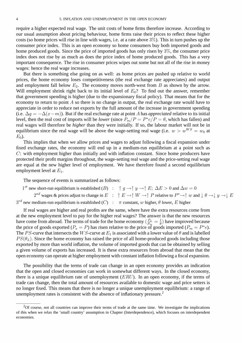
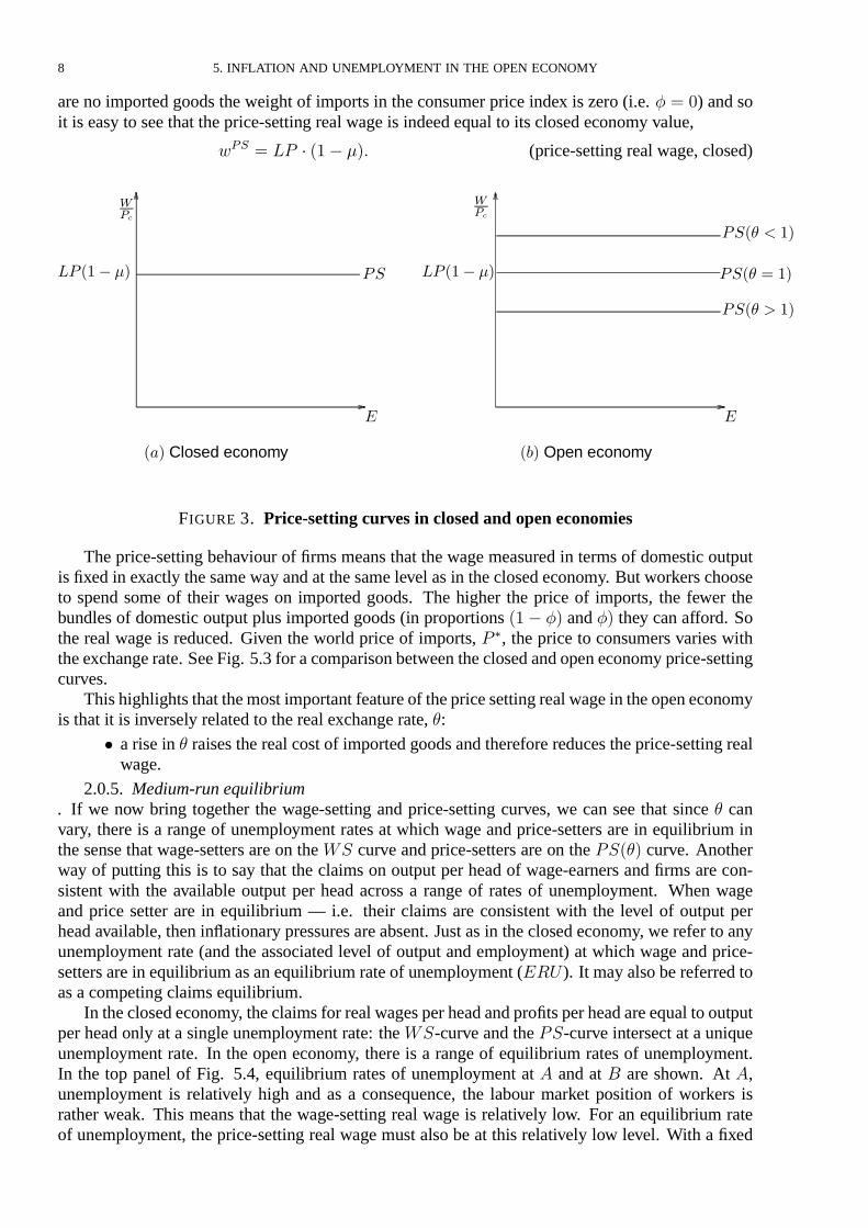
are no imported goods the weight of imports in theconsumer price index is zero (i.e. � � �) and soit is easy to see that theprice-setting real wage is indeed equal to itsclosed economy value,

�� (price-setting real wage, closed)

�

��

� � Closed economy

��

��

�

��

��

��

�� Open economy

��

��

FIGURE 3. Price-setting curves in closed and open economies

The price-setting behaviour of firms means that the wage measured in terms of domestic outputisfixed in exactly thesameway and at thesamelevel as in theclosed economy. But workerschooseto spend some of their wages on imported goods. The higher the price of imports, the fewer thebundles of domestic output plus imported goods (in proportions �� and �� they can afford. Sothe real wage is reduced. Given the world price of imports, � �, the price to consumers varies withtheexchangerate. SeeFig. 5.3 for acomparison between theclosed and open economy price-settingcurves.

Thishighlightsthat themost important featureof thepricesetting real wagein theopen economyis that it is inversely related to the real exchange rate, �:

� arise in � raises the real cost of imported goodsand therefore reduces theprice-setting realwage.

2.0.5. Medium-run equilibrium. If we now bring together the wage-setting and price-setting curves, we can see that since � canvary, there is a range of unemployment rates at which wage and price-setters are in equilibrium inthe sense that wage-setters are on the curve and price-setters are on the�� curve. Anotherway of putting this is to say that the claims on output per head of wage-earners and firms are con-sistent with the available output per head across a range of rates of unemployment. When wageand price setter are in equilibrium — i.e. their claims are consistent with the level of output perhead available, then in�ationary pressuresareabsent. Just as in theclosed economy, werefer to anyunemployment rate (and the associated level of output and employment) at which wage and price-settersare in equilibrium asan equilibrium rateof unemployment (�� ). It may also bereferred toas acompeting claims equilibrium.

In theclosed economy, theclaimsfor real wagesper head and profitsper head areequal to outputper head only at a single unemployment rate: the-curve and the�-curve intersect at auniqueunemployment rate. In the open economy, there is a range of equilibrium rates of unemployment.In the top panel of Fig. 5.4, equilibrium rates of unemployment at � and at � are shown. At �,unemployment is relatively high and as a consequence, the labour market position of workers israther weak. This means that the wage-setting real wage is relatively low. For an equilibrium rateof unemployment, the price-setting real wage must also be at this relatively low level. With a fixed


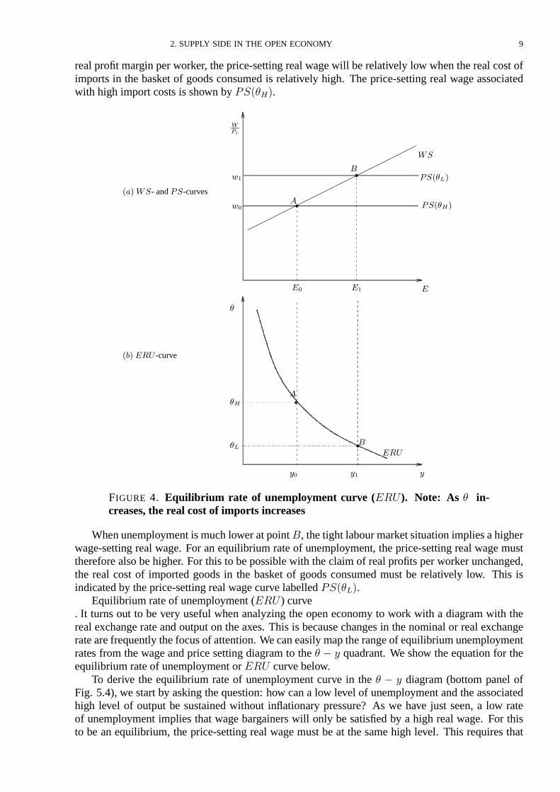
real profit margin per worker, theprice-setting real wagewill be relatively low when the real cost ofimports in the basket of goods consumed is relatively high. The price-setting real wage associatedwith high import costs isshown by ��.

��

��

��

��

��

��

��

��

��

��

�� -curve

��

�

��

��

� �

��- and��-curves

�

�

��

��

��

�

�

��

�

��

�

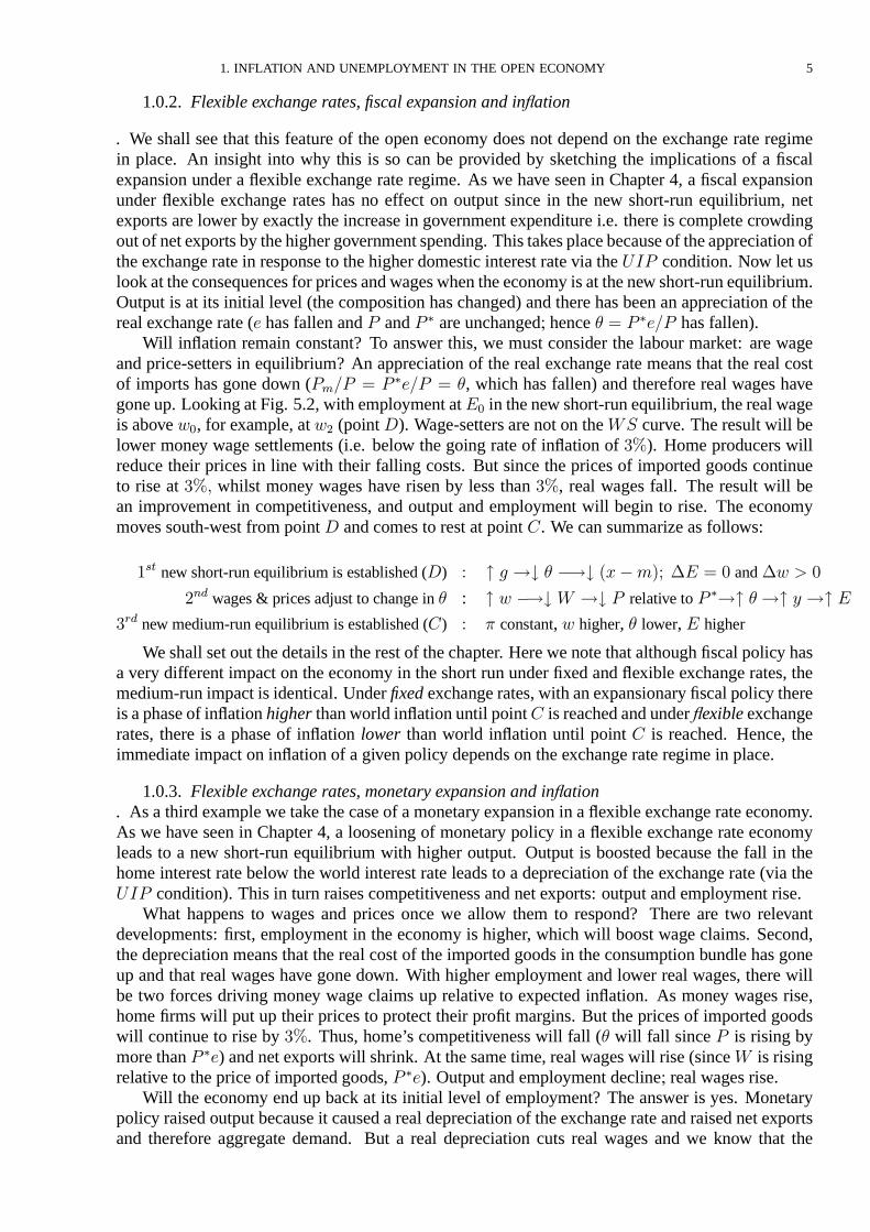
FIGURE 4. Equilibr ium rate of unemployment curve (��). Note: As � in-creases, the real cost of imports increases

When unemployment ismuch lower at point �, thetight labour market situation impliesahigherwage-setting real wage. For an equilibrium rate of unemployment, the price-setting real wage musttherefore also behigher. For this to bepossiblewith the claim of real profits per worker unchanged,the real cost of imported goods in the basket of goods consumed must be relatively low. This isindicated by theprice-setting real wagecurve labelled �� .

Equilibrium rateof unemployment (�� ) curve. It turns out to be very useful when analyzing the open economy to work with a diagram with thereal exchange rate and output on the axes. This is because changes in the nominal or real exchangeratearefrequently thefocusof attention. Wecan easily map therangeof equilibrium unemploymentrates from the wage and price setting diagram to the � � � quadrant. We show the equation for theequilibrium rateof unemployment or �� curvebelow.

To derive the equilibrium rate of unemployment curve in the � � � diagram (bottom panel ofFig. 5.4), we start by asking the question: how can a low level of unemployment and the associatedhigh level of output be sustained without in�ationary pressure? As we have just seen, a low rateof unemployment implies that wage bargainers will only be satisfied by a high real wage. For thisto be an equilibrium, the price-setting real wage must be at the same high level. This requires that


the real cost of imported goods is sufficiently low. At point � in the top panel of Fig.5.4 there is ahigh value of employment — and therefore a high level of output. This means that for equilibriumin the labour market, we have to have a low value of � so that import costs are low (see point � inthe bottom panel). A low value of � � ��

�means that the world price level and hence the price of

imported goods (� � � is low relative to thepriceof homegoodsand henceof exports (� ). With lowimport costs, real wages can behigh without affecting the real valueof profits. Living standards areboosted because imports are cheap. This gives point � at the combination of a low valueof � and ahigh level of output.

Exactly the same logic lies behind the location of point �. When unemployment is high andoutput is depressed, workers are in a weak position in the labour market and there is a low wage-setting real wage. For the price-setting real wage to be at this low level as is required for competingclaimsequilibrium, thecost of imported goodsmust behigh. At point � therewill beacombinationof low output and high import costs, i.e. high �. Hence the equilibrium rate of unemployment(�� ) curve in the� � � diagram is downward sloping (bottom panel of Fig. 5.4).

DEFINITION 1 (Equilibrium Rate of Unemployment curve). The �� -curve is defined as thecombinations of the real exchange rate and output at which the wage-setting real wage is equal tothe price-setting real wage. At any point on the�� -curve, the real exchange rate, �� is constantand in�ation is constant.

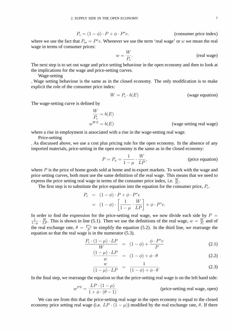
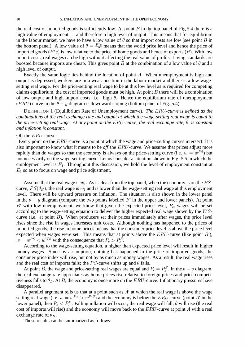
Off the�� -curve. Every point on the�� -curve isapoint at which thewageand price-setting curves intersect. It isalso important to know what it means to be off the�� -curve. We assume that prices adjust morerapidly than do wages so that the economy is always on the price-setting curve (i.e. � � ��) butnot necessarily on thewage-setting curve. Let usconsider asituation shown in Fig. 5.5 in which theemployment level is ��. Throughout this discussion, we hold the level of employment constant at�� so as to focus on wageand price adjustment.

Assumethat thereal wageis��. As isclear from thetop panel, when theeconomy ison the�-curve, �� the real wageis�� and is lower than thewage-setting real wageat thisemploymentlevel. There will be upward pressure on in�ation. The situation is also shown in the lower panelin the � � � diagram (compare the two points labelled �� in the upper and lower panels). At point�� with low unemployment, we know that given the expected price level, �� wages will be setaccording to the wage-setting equation to deliver the higher expected real wage shown by the-curve (i.e. at point �). When producers set their prices immediately after wages, the price levelrises since the rise in wages increases unit costs. Although nothing has happened to the prices ofimported goods, the rise in home prices means that the consumer price level is above theprice levelexpected when wages were set. This means that at points above the �� -curve (like point ��),� � �� with theconsequence that ��

� .According to the wage-setting equation, a higher than expected price level will result in higher

money wages. Since by assumption, nothing has happened to the price of imported goods, theconsumer price index will rise, but not by as much as money wages. As a result, the real wage risesand the real cost of imports falls: the�-curveshifts up and � falls.

At point �, thewageand price-setting real wagesareequal and �� In the� � � diagram,

the real exchange rate appreciates as home prices rise relative to foreign prices and price competi-tiveness falls to � � At �, theeconomy isoncemoreon the�� -curve. In�ationary pressureshavedisappeared.

A parallel argument tells us that at a point such as�� at which the real wage is above the wagesetting real wage(i.e. � � �� and theeconomy isbelow the�� -curve(point �� in thelower panel), then ��

� . Falling in�ation will occur, the real wage will fall, � will rise (the realcost of imports will rise) and the economy will move back to the�� -curve at point � with a realexchange rateof ��

These resultscan besummarized as follows:


��

��

��

��

��

��

��

�

��

�

��

��

� �

��

��

�

� �

�

�

�

��

�

��

��

�

��

��

��

��

�

FIGURE 5. Off the�� -curve

� On the�� -curve, in�ation isconstant.� At pointsabove the��-curve, the real wage isbelow the-curveso that homewages

and prices are rising relative to those abroad. Home in�ation is rising relative to worldin�ation. Hence� is falling.

� At pointsbelow the�� -curve, thereal wage isabove the-curveso that homewagesand prices are falling relative to those abroad. Home in�ation is falling relative to worldin�ation. Hence� is rising.

Slopeof the��-curve. A glance at Fig. 5.5 suggests that the steepness of the��-curve will be very important in fixingthe range of output and employment levels consistent with stable in�ation. If the��-curve wasvertical, then there would be a unique equilibrium unemployment rate — a very steep �� -curvewould display only a narrow range of unemployment equilibria. A steep ��-curve means that avery large change in the real exchange rate is required to bring about the change in the real cost ofimports that is necessary to allow the wage and price setting real wage to be equal at a higher levelof employment. Thiscould bebecause the import propensity is very small so that avery big changein relativeprices isneeded to alter the real cost of imports in theconsumption bundle.

It couldalsobebecausethewage-setting real wageisvery steep, i.e. real wagesarevery sensitiveto a change in unemployment. In such a case, a given fall in unemployment leads to a very big risein thewage-setting real wageand hencefor agiven import propensity, requiresa largecut in therealcost of imports (fall in �) to allow thenecessary rise in theprice-setting real wage.


By contrast, a �at �� -curve would indicate a wide range of medium-run equilibria. In thiscase, a high import share would mean that only a small fall in � would be required for competingclaims equilibrium at lower unemployment. Equally, if real wages are rather insensitive to em-ployment, then a given fall in unemployment will be associated with only a modest rise in thewage-setting real wage along the-curve and therefore only a small fall in � is needed to ensurecompeting claims equilibrium at lower unemployment. (Details for sketching the �� curve areshown in the Appendix to this chapter.)

To summarize:(1) If theeconomy is closed so that thereare no imports (i.e. � � �), there is aunique equilib-

rium level of output and henceauniqueequilibrium unemployment rate. Thiswill defineavertical �� -curve.

(2) As the share of imports rises, the�� -curve becomes�atter. More open economies have�atter �� -curves.

(3) If the wage setting curve is �atter (i.e. real wages are less sensitive to employment), thiswill make the�� -curve�atter. Economies in which labour market institutions make thewage-setting real wage more insensitive to changes in unemployment have �atter ��-curves.

3. Demand sideand tradebalance

In Chapter 4, weintroduced theimpact on themacroeconomy of opennessin goodsand financialmarkets. The task now is to translate thekey featuresof goodsand financial market equilibrium andof tradebalance into thenew � � � diagram. This step prepares theground for Section 5.3 in whichthe supply side, the demand side and the trade balance are brought together to form the basic openeconomy model. Weshall see that using the� � � diagram greatly clarifiesopen economy analysis.Asusual weassumethat theMarshall–Lerner condition holdsso that a rise in pricecompetitiveness(a real exchange ratedepreciation) boosts the tradebalance (holding the level of output constant).

Goodsmarket equilibrium issummarized by:

� � ��

� � ��

� � �� !��

and � ��

Notethat weassumethat thehome real interest rate isequal to theexogenousworld real interestrate. In effect, we are assuming that the Mundell-Fleming adjustment process, discussed in detailin Chapter 4, has brought the economy to a short-run equilibrium. For now the focus is on themedium-run. Figure6 shows theconstruction of the�� curve in the� � � diagram.

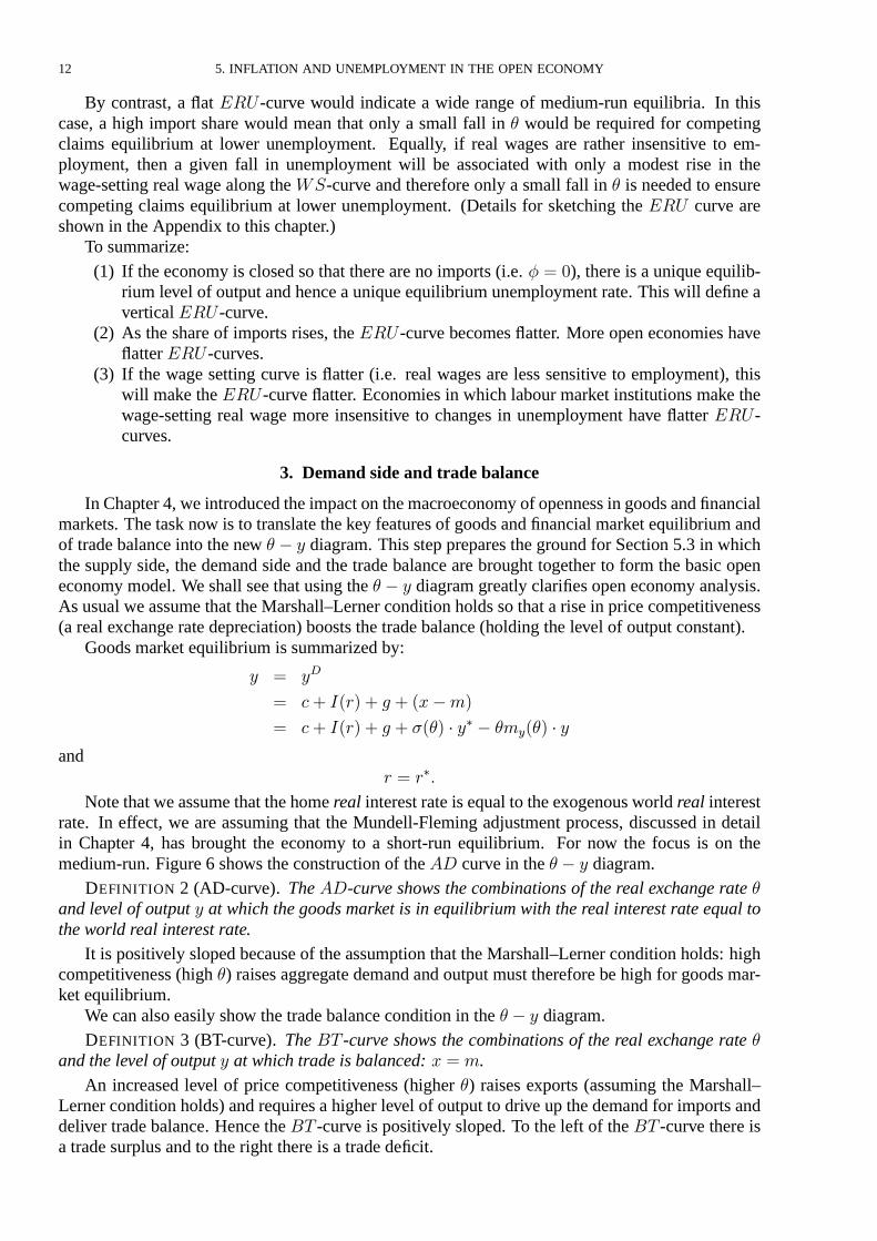
DEFINITION 2 (AD-curve). The��-curve shows the combinations of the real exchange rate �and level of output � at which thegoods market is in equilibriumwith the real interest rate equal totheworld real interest rate.

It is positively sloped becauseof theassumption that theMarshall–Lerner condition holds: highcompetitiveness (high �) raises aggregatedemand and output must thereforebe high for goodsmar-ket equilibrium.

Wecan also easily show the tradebalancecondition in the � � � diagram.DEFINITION 3 (BT-curve). The �" -curve shows the combinations of the real exchange rate �

and the level of output � at which trade isbalanced: � � �.

An increased level of price competitiveness (higher �) raises exports (assuming the Marshall–Lerner condition holds) and requiresahigher level of output to driveup thedemand for importsanddeliver tradebalance. Hence the�" -curve is positively sloped. To the left of the�" -curve there isa tradesurplus and to the right there isa tradedeficit.

3. DEMAND SIDE AND TRADE BALANCE 13

��

��

�

�

��

surplus

deficit

�

� �

��

��

�

��

��

��

��

��

�

FIGURE 6. Short-run equilibr ium (goods & money market): ��-curve� andtradeequilibr ium: �" -curve

The�" -curve is�atter than the��-curve. The underlying reason for this result was explainedin detail in Section 4.1, Fig. 4.3 when we asked what the outcome for the balance of trade wouldbe if there was a depreciation of the real exchange rate. The answer was that there would be a tradesurplus: this is shown by point � in Fig.5.6. The intuition is that from an initial equilibrium atpoint � at which trade is balanced, a given increase in � implies a new goods market equilibriumat point �� where the level of output is lower than would be consistent with trade balance. This isbecause there are leakages in the form of savings and taxation (in addition to imports). This leavesthe economy in goods market equilibrium at a level of output below the level that would generateimportsequal to thenew higher level of exports.

A senseof theusefulnessof thenew �� diagram isconveyed by thefollowing exercise.4 Thinkof a government that has two targets for economic policy — high output and external balance, asdefined by trade balance. The government has two instruments of economic policy — the nominalexchange rate and fiscal policy (remember that � �). There are two relationships linking thetargetsand the instruments: the�#$ equilibrium (with � �� summarized in the�� curveandthebalanceof tradecurve, �" .

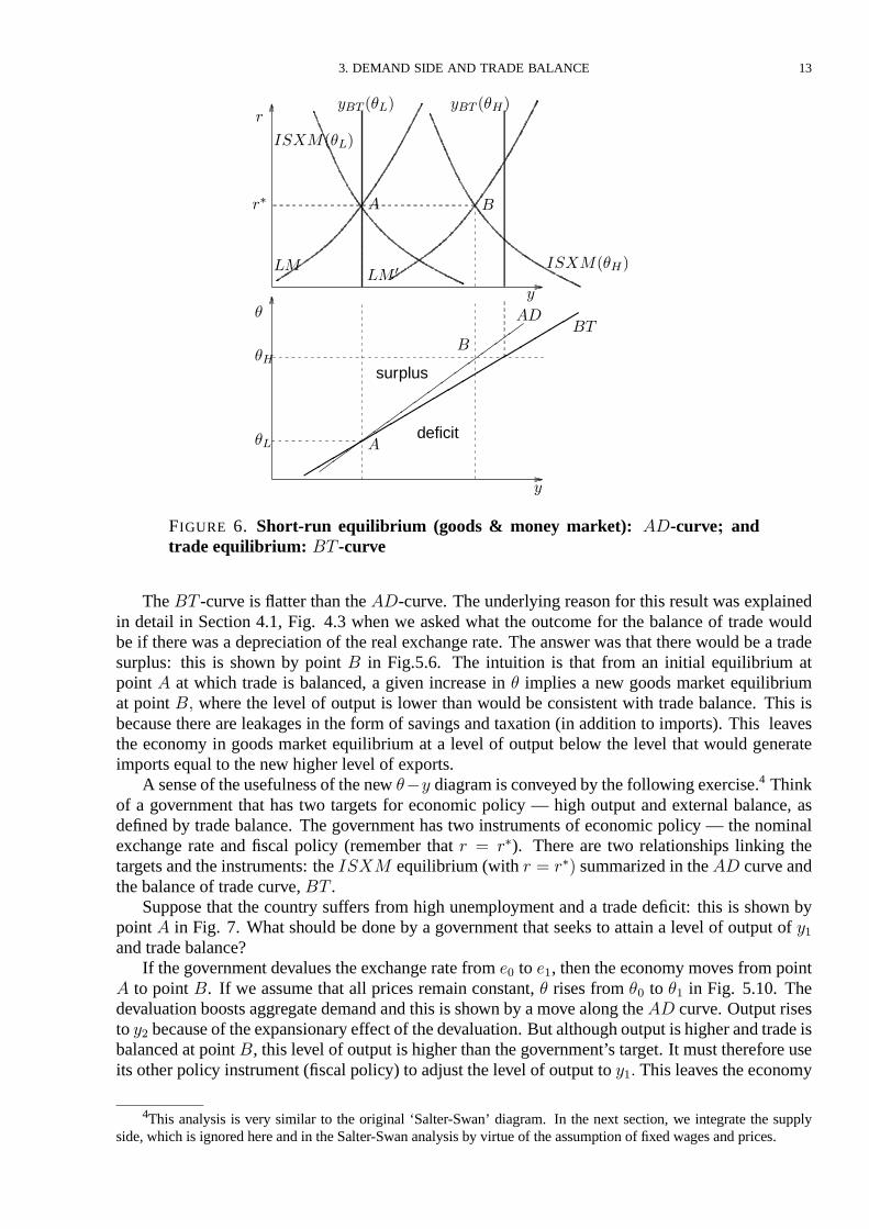
Suppose that the country suffers from high unemployment and a trade deficit: this is shown bypoint � in Fig. 7. What should be done by a government that seeks to attain a level of output of ��and tradebalance?

If thegovernment devalues theexchangerate from � to �, then theeconomy moves from point� to point �. If we assume that all prices remain constant, � rises from �� to �� in Fig. 5.10. Thedevaluation boostsaggregatedemand and this isshown by amovealong the�� curve. Output risesto �� becauseof theexpansionary effect of thedevaluation. But although output ishigher and tradeisbalanced at point �, this level of output ishigher than thegovernment’s target. It must thereforeuseitsother policy instrument (fiscal policy) to adjust the level of output to �� This leaves theeconomy

4This analysis is very similar to the original ‘Salter-Swan’ diagram. In the next section, we integrate the supplyside, which is ignored hereand in theSalter-Swan analysisby virtueof theassumption of fixed wagesand prices.


��

��

��

�

�"

� �

��

��

devaluation

�

��

��

�

FIGURE 7. Use of a devaluation and fiscal policy to achieve target output level,��, and tradebalance

at point � with the desired output level and with balanced trade. In this example, contractionaryfiscal policy is combined with adevaluation.

In thisexample, wehaveseen how it will generally benecessary to use two instruments in orderto achieve the government’s two targets of “ internal” and “external” balance. But is position �really a position of internal balance? What does the level of the real exchange rate at � imply forthe real wage? Is this real wage compatible with wage-setting behaviour in the economy? Thesequestions signal that we must bring the supply and the demand sides of the economy together withthetradebalancecondition in order to fully assessthecharacteristicsof apoint such as� with targetunemployment and balanced trade. Wedo this in thenext section by putting together thebasic openeconomy model.

4. Basic open economy model

Thebasic model for analysis in thesmall open economy consists of

� the demand side represented by the ��-curve. On the ��-curve, the goods market is inequilibrium and � �.

� the supply side represented by the�� -curve. On the��-curve in�ation is constant.� the balanceof tradeequilibrium represented by the�" -curve.

In theshort run, theeconomy will beon the��-curve in goodsmarket equilibrium. For agivennominal exchange rateand agiven price level, the level of output isfixed by the��-curve. But thisisnot necessarily amedium-run equilibrium.

For medium-run equilibrium, theeconomy must also beon the��-curve. Only on the��-curve are the wage and price setting real wages equal and in�ationary or disin�ationary pressuresabsent. In themedium run, therefore, the economy will beon an ��-curveand on the�� -curve.

Only by chance will the medium-run equilibrium also be characterized by trade balance. Long-run equilibrium is at a position on the��-curve and at current account balance. As we haveseenin Chapter 4, when the current account is balanced, the country’s wealth is constant. To make theexposition assimpleas possible, we ignore thedifferencebetween the tradebalanceand thecurrentaccount. Thisallowsusto define the long-run equilibrium asthe intersection of the��-curveandthe �" -curve. We are using long run in the macroeconomic sense — i.e. holding the economy’scapital stock constant. As is usual in macroeconomics, weareabstracting from growth.

4. BASIC OPEN ECONOMY MODEL 15

As discussed in Chapter 4, in the long run, there may be pressures that tend to ensure thatthere is trade balance in the economy. Such pressures can arise from private sector changes inaggregate demand through the wealth effects on consumption expenditure associated with a tradesurplus (home wealth is rising) or a trade deficit (home wealth is falling). Equally, pressure maymount in the foreign exchangemarket and force thegovernment to change its policy.

��

��

��

��

��

��

��

�

�

�

��

�

�

��

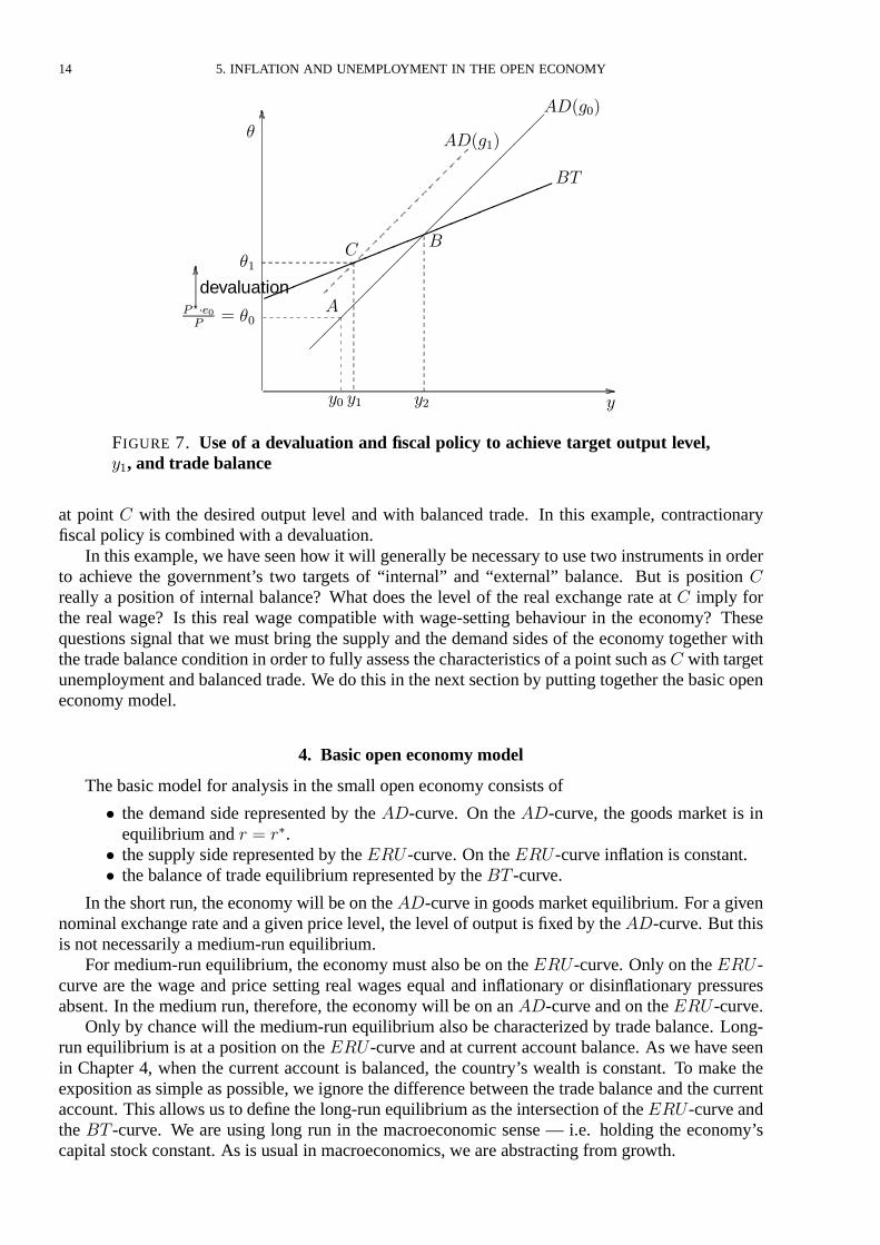
FIGURE 8. Shor t-run, medium-run and long-run equilibr ia in theopen economy

The difference between short, medium and long-run equilibria in the basic model is illustratedby theexample in Fig. 8. Let us compare thecharacteristicsof points�, �� and %�

: Short-runequilibriumat point � — on�� but not on�� or �" . At point �, theeconomyis on the ��-curve and the level of output is ��. The real exchange rate is equal to ��and the economy is above the ��-curve. This means that the prevailing real wage isbelow the real wage that wage-setters can expect at the relatively low unemployment rateassociated with ��. Workers are in a rather strong position in the labour market and themoney wage that is set will rise relative to the expected price level. Home prices will riserelative to foreign prices. In�ation is rising relative to world in�ation. This depressespricecompetitiveness and theeconomy moves along the��-curve toward point �. Output fallsbecauseof the lower export demand generated by the fall in competitiveness.

: Medium-run equilibriaat points� and��— on�� and�� and�� respectively but noton �" . In�ation is constant at points� and �� because each is on the�� -curve. Thereis a trade surplus at point � because it is to the left of the �" -curve and a trade deficitat point �� because it is to the right of the �" -curve. The economy can remain at pointslike� and �� with stable in�ation. However, in the longer run, pressures may emerge as aconsequenceof thetradeposition that tend to push theeconomy away from� or �� towardpoint %�

: Long-run equilibrium at point % — on ��, �� and �" . At point %, the competingclaims equilibrium coincides with the balanced trade level of output. This is likely to be asustainable long run position for theeconomy.

Having put together the basic open economy model, we can now reexamine the situation de-scribed in Fig. 7 above: recall that the government used its two policy instruments of a change inthe exchange rate and an adjustment of fiscal policy to achieve its two targets, the desired outputlevel of �� and trade balance. We asked the following questions: Is position � really a position ofinternal balance? What does the level of the real exchange rateat � imply for the real wage? Is this


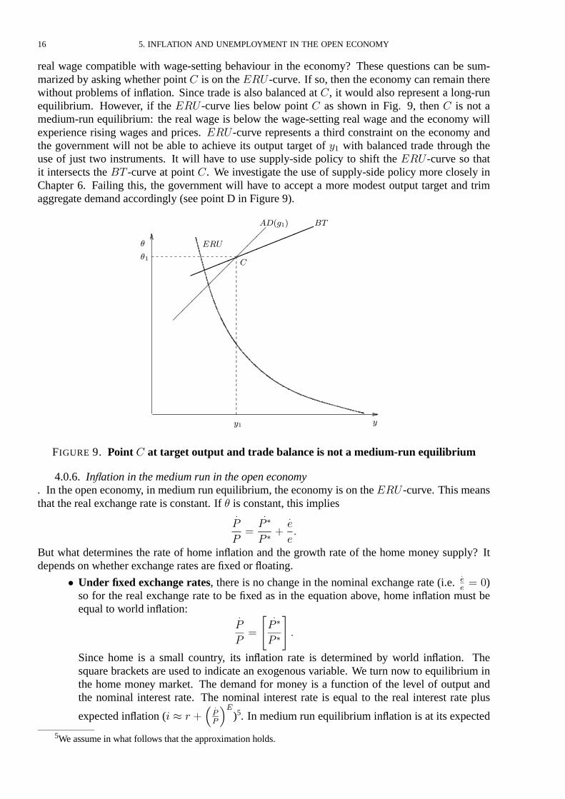
real wage compatible with wage-setting behaviour in the economy? These questions can be sum-marized by asking whether point � is on the�� -curve. If so, then theeconomy can remain therewithout problems of in�ation. Since trade is also balanced at �, it would also represent a long-runequilibrium. However, if the �� -curve lies below point � as shown in Fig. 9, then � is not amedium-run equilibrium: the real wage is below the wage-setting real wage and the economy willexperience rising wages and prices. ��-curve represents a third constraint on the economy andthe government will not be able to achieve its output target of �� with balanced trade through theuse of just two instruments. It will have to use supply-side policy to shift the ��-curve so thatit intersects the�" -curve at point �. We investigate the use of supply-side policy more closely inChapter 6. Failing this, the government will have to accept a more modest output target and trimaggregatedemand accordingly (seepoint D in Figure9).

��

��

��

��

�

�

�

��

FIGURE 9. Point � at target output and tradebalance is not a medium-run equilibr ium

4.0.6. In�ation in themediumrun in theopen economy. In theopen economy, in medium run equilibrium, theeconomy ison the�� -curve. Thismeansthat the real exchange rate isconstant. If � is constant, this implies

�

�

��

�

� �

� �

�

�

But what determines the rate of home in�ation and the growth rate of the home money supply? Itdependson whether exchange ratesarefixed or �oating.

� Under fixed exchange rates, there is no change in the nominal exchange rate (i.e.�� )

so for the real exchange rate to be fixed as in the equation above, home in�ation must beequal to world in�ation:

�

�

��

� �

� �

� �

�

�

Since home is a small country, its in�ation rate is determined by world in�ation. Thesquare brackets are used to indicate an exogenous variable. We turn now to equilibrium inthe home money market. The demand for money is a function of the level of output andthe nominal interest rate. The nominal interest rate is equal to the real interest rate plus

expected in�ation (� � � �

��

��)5. In medium run equilibrium in�ation is at its expected

5Weassumein what follows that theapproximation holds.

4. BASIC OPEN ECONOMY MODEL 17

rate. With in�ation at theworld rateand with thehome real interest rateequal to theworldrate ( � �), equilibrium in thehome money market is as follows:

�$

�

��

�$

�

��

� ��

� ��

�

�

�

��

� ��

�

��

� ��

In medium run, equilibrium in the home money market implies that the real moneysupply, �

�� is constant sinceall thedeterminantsof thedemand for money arefixed. Hence

thehomemoney supply is endogenousand must grow at thesamerateas in�ation:�

$

$�

�

�

��

� �

� �

� �

�

� (fixed exchange rates)

Thus as long as foreign in�ation remains constant and the exchange rate is fixed, homein�ation is constant at the foreign rate in medium-run equilibrium. We assume constantworld in�ation.

� Under �exible exchange rates, in medium run equilibrium, it is also the case that the realexchange rate, �, is constant. Hence

�

�

��

�

� �

� �

�

�

For equilibrium in thehomemoney market and with thehomereal interest rateequal totheworld rate ( � �),

�$

�

��

�$

�

��

� ��

� ��

�

�

�

��

At the medium run output level, in�ation is constant at its expected rate. This implies thatthehomemoney supply must grow at therateof homein�ation. Weassumethat thegrowthrateof thehomemoney supply is exogenous, this determines the rateof home in�ation.

� �

$

$

�

�

�

�

��

Thechange in the nominal exchange rate is endogenous: it is determined by thedifferencebetween thegrowth rateof thehomemoney supply (and hencehomein�ation) and therateof world in�ation:

�

�

�

�

��

� �

� �

� �

�

(�exibleexchange rates)

�

� �

$

$

�

�

� �

� �

� �

�


In medium run equilibrium in the�exibleexchange rateeconomy, thereal exchange rate isconstant, in�ation is constant and the nominal exchange rate is changing unless home andworld in�ation are the same.

Summing up. In the open economy, there is a range of output and employment levels consistent

with constant home in�ation in the medium run. There is no unique �� . The economy can beat any point on the�� -curve with constant in�ation equal to the growth rate of the home moneysupply — this is set by world in�ation in the fixed exchange rate economy and by the home centralbank in the�exibleexchange rateeconomy.

5. Long-run equilibr ium

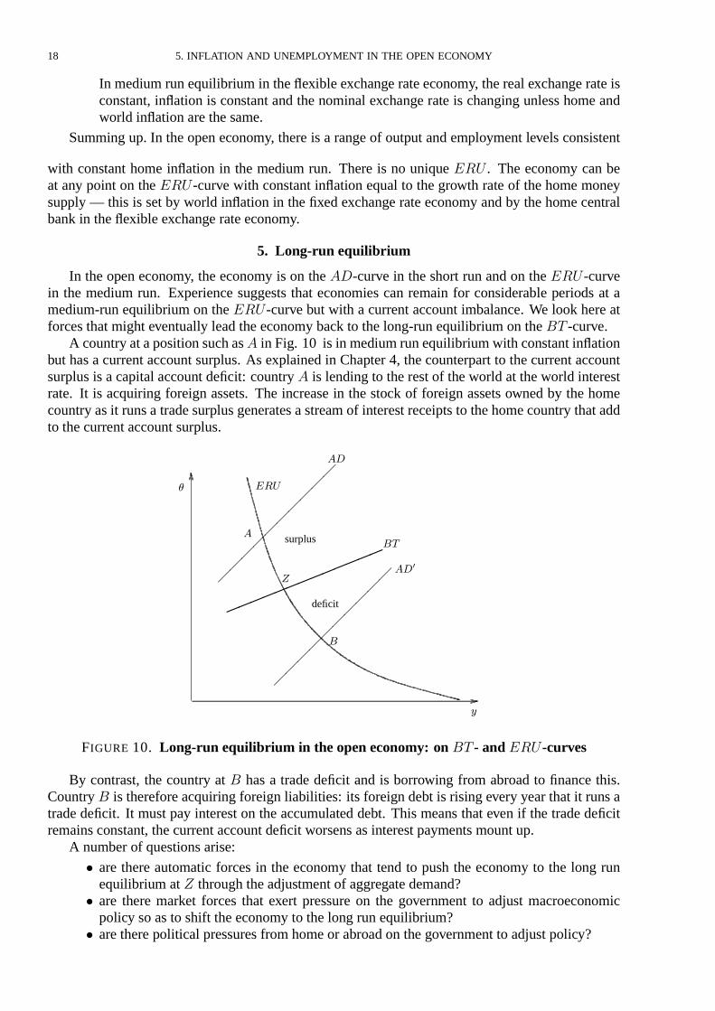
In the open economy, the economy is on the��-curve in the short run and on the�� -curvein the medium run. Experience suggests that economies can remain for considerable periods at amedium-run equilibrium on the��-curve but with a current account imbalance. We look here atforces that might eventually lead the economy back to the long-run equilibrium on the�" -curve.

A country at aposition such as� in Fig. 10 is in medium run equilibrium with constant in�ationbut has a current account surplus. As explained in Chapter 4, the counterpart to the current accountsurplus is acapital account deficit: country � is lending to the rest of theworld at theworld interestrate. It is acquiring foreign assets. The increase in the stock of foreign assets owned by the homecountry as it runsa tradesurplusgeneratesastream of interest receipts to thehomecountry that addto thecurrent account surplus.

��

��

��

��

��

��

��

�

�

�

surplus

deficit

�

FIGURE 10. Long-run equilibr ium in theopen economy: on �" - and �� -curves

By contrast, the country at � has a trade deficit and is borrowing from abroad to finance this.Country � is thereforeacquiring foreign liabilities: its foreign debt is rising every year that it runsatrade deficit. It must pay interest on the accumulated debt. This means that even if the trade deficitremainsconstant, thecurrent account deficit worsens as interest payments mount up.

A number of questions arise:

� are there automatic forces in the economy that tend to push the economy to the long runequilibrium at % through theadjustment of aggregatedemand?

� are there market forces that exert pressure on the government to adjust macroeconomicpolicy so as to shift theeconomy to the long run equilibrium?

� are there political pressures from homeor abroad on the government to adjust policy?

5. LONG-RUN EQUILIBRIUM 19

We first examine these three mechanisms that might push the economy toward the long-runequilibrium (where the�� and �" curves intersect). At thisstage, weassumethat exchangerateexpectations are stable — i.e. that they are not affected by the trade position. In a second step, welook at how theeconomy may shift toward the long-run equilibrium as aconsequenceof the impactof the tradeposition on exchange rateexpectations.

5.1. Mechanisms with stableexchange rateexpectations.Wealth effects. One automatic mechanism that might produce a shift to long-run equilibrium is the operation ofwealth effects. As noted in Chapter 4, home consumers may incorporate the changes in nationalwealth into their consumption decisions. It is obvious that a country cannot run down its wealthindefinitely: far-sighted consumers in the deficit country, �, may take the view that the deficit doesnot re�ect a programme of investment in the home economy that will bear fruit in the longer term.They may believe that belt-tightening will eventually be required in the home economy to serviceand repay the foreign debt. As a result, they may adjust downward their estimate of permanentincomeand implement theassociated cut in consumption spending. For acountry such ascountry �with a trade surplus, the opposite considerations may lead to a rise in the assessment of permanentincomeand henceconsumption may increase. To theextent that thesereactionsoccur, the��-curvewill shift toward the long run equilibrium. These forcesaloneareunlikely to bepowerful enough toguarantee long-run equilibrium.Market pressure. Throughout the analysis of the open economy in this chapter, we have made the assumption ofperfect international capital mobility. Countries can borrow indefinitely at the international interestrate. But acountry with apersistent tradedeficit facesabuild-up of its foreign debt. Asnoted above,it ispossiblethat thedeficit arisesfrom thecountry taking advantageof especially favourable invest-ment opportunities at home by borrowing from abroad. If so, then the investments will eventuallybear fruit and directly or indirectly improvethecountry’sexport baseallowing it to movefrom tradedeficit to tradesurplusand repay itsdebt. Norway providesan illustration of thispattern: thereweresubstantial current account deficits averaging nearly 5% of GDP from the mid 1970s and into the1980s as the domestic oil industry was developed, which were followed by surpluses in the1990s.

If the sentiment in international financial markets is that the trade deficit re�ects high homeconsumption or wasteful investment, then fundswill cease to beavailable to country � at theworldinterest rate. Private expenditure will tend to be dampened by the change in credit conditions. Inaddition, the government may implement a tightening of aggregate demand policy to reduce thetradedeficit.Political pressure. The economic pressures on deficit countries to adjust are typically stronger than those on surpluscountries. If wealth effectson consumption areweak, then acountry isableto run atradesurplusfora lengthy period of time. Thissuggests theremay bean asymmetry between deficit countries like�and surplus countries like�. Unless the investment opportunities abroad are particularly profitable,thewisdom of running a persistent surplus isquestionable. This may lead to political pressure fromwithin the country for the government to boost activity and operate at a lower unemployment rate.Surplus countries can also come under political pressure at the international level to adjust theirpolicies (e.g. the US exerted pressureon theJapaneseauthoritiesduring the1980s).

5.2. Unstableexchange rateexpectations. In the basic open economy model, we assumethattheexchangerateremainsat itsexpected level and that expectationsareformed in asimplebackwardlooking way. But even under fixed exchange rates, acountry with apersistent tradedeficit may findit difficult to defend theexchangeratepeg indefinitely. Asdiscussed in Chapter 4, if privatecounter-partiesarenot willing to purchasethehomecurrency and financethedeficit, then thehomecountry’scentral bank will have to sell foreign exchange reserves. There is a limit to the extent to which thisispossiblebecauseforeign exchangereservesare limited and borrowing to supplement them may be


difficult. Onceexchangemarket operatorsbegin to speculateon adevaluation, thecentral bank maybe forced to combine interest rate rises to try to hold the exchange rate peg with intervention in theforeign exchangemarket. Eventually, thegovernment may beforced to tighten fiscal policy to movethe economy toward the long run equilibrium. Policy combinations are examined in more detail inChapter 11.

Under �exible exchange rates, the stability of a medium run equilibrium is an open question.There is no consensus about the sustainability of a medium run equilibrium because the process bywhich exchangemarket expectations are formed is not well understood.

The aim of this section is to show that if we take a very different expectations hypothesis fromthe standard one in the basic model, then the results can change dramatically. For example, let ussuppose that the exchange rate is expected to adjust immediately to deliver a real exchange rateconsistent with trade balance i.e.

� � �� if and only if �" � ��

If there is a trade deficit, the exchange rate is expected to depreciate and if there is a trade surplus,theexchange rate is expected to appreciate.

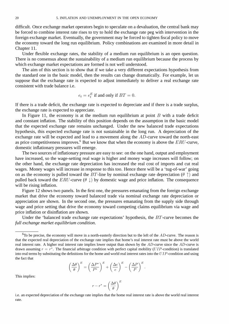
In Figure 11, the economy is at the medium run equilibrium at point � with a trade deficitand constant in�ation. The stability of this position depends on the assumption in the basic modelthat the expected exchange rate remains unchanged. Under the new balanced trade expectationshypothesis, this expected exchange rate is not sustainable in the long run. A depreciation of theexchange rate will be expected and lead to a movement along the ��-curve toward the north-eastas price competitiveness improves.6 But we know that when theeconomy is above the�� -curve,domestic in�ationary pressures will emerge.

Thetwo sourcesof in�ationary pressureareeasy to see: on theonehand, output and employmenthave increased, so the wage-setting real wage is higher and money wage increases will follow� onthe other hand, the exchange rate depreciation has increased the real cost of imports and cut realwages. Money wages will increase in response to this too. Hence therewill bea ‘ tug-of-war’ goingon as the economy is pulled toward the �" -line by nominal exchange rate depreciation (� �� andpulled back toward the �� -curve (� �� by domestic wage and price in�ation. The consequencewill be rising in�ation.

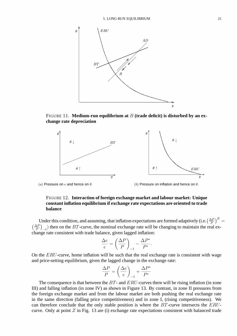
Figure12 shows two panels. In thefirst one, thepressuresemanating from the foreign exchangemarket that drive the economy toward balanced trade via nominal exchange rate depreciation orappreciation are shown. In the second one, the pressures emanating from the supply side throughwage and price setting that drive the economy toward competing claims equilibrium via wage andprice in�ation or disin�ation areshown.

Under the ‘balanced trade exchange rate expectations’ hypothesis, the �" -curve becomes thefull exchangemarket equilibriumcondition.

6To be precise, the economy will move in a north-easterly direction but to the left of the�-curve. The reason isthat the expected real depreciation of the exchange rate implies that home’s real interest rate must be above the worldreal interest rate. A higher real interest rate implies lower output than shown by the�-curve since the�-curve isdrawn assuming � � ��. The financial arbitrage condition with perfect capital mobility (�� -condition) is translatedinto real termsby substituting thedefinitionsfor thehomeand world real interest ratesinto the�� -condition and usingthe fact that

��

�

��

��

� �

��

��

�

��

��

�

��

This implies:

� � ��

��

�

��

i.e. an expected depreciation of theexchangerate implies that thehomereal interest rate isabove theworld real interestrate.

5. LONG-RUN EQUILIBRIUM 21

��

��

��

��

��

��

��

�

�

FIGURE 11. Medium-run equilibr ium at � (tradedeficit) isdisturbed by an ex-change ratedepreciation

��

��

��

�

� �

��

�� Pressure on in�ation and hence on �.

�

� �

� �

�

��

�� Pressure on � and hence on �.

FIGURE 12. Interaction of foreign exchangemarket and labour market: Uniqueconstant in�ation equilibr ium if exchangerateexpectationsareor iented to tradebalance

Under thiscondition, andassuming, that in�ationexpectationsareformedadaptively (i.e.��

��

��

�� then on the�" -curve, thenominal exchangeratewill bechanging to maintain thereal ex-

change rateconsistent with tradebalance, given lagged in�ation:

�

�

��

�

�

��

��

� ��

On the�� -curve, home in�ation will be such that the real exchange rate is consistent with wageand price-setting equilibrium, given the lagged change in theexchange rate:

��

��

��

�

��

��

� �

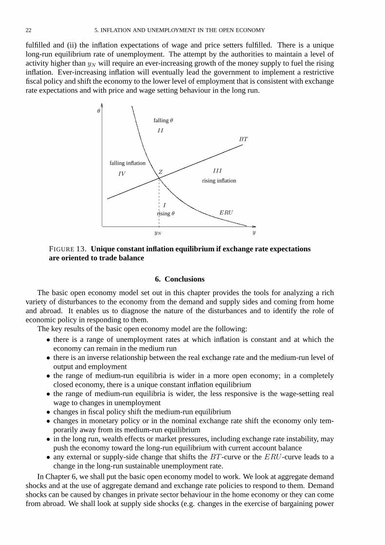
Theconsequenceis that between the�" - and��-curvestherewill berising in�ation (in zoneIII) and falling in�ation (in zone IV) as shown in Figure 13. By contrast, in zone II pressures fromthe foreign exchange market and from the labour market are both pushing the real exchange ratein the same direction (falling price competitiveness) and in zone I, (rising competitiveness). Wecan therefore conclude that the only stable position is where the �" -curve intersects the ��-curve. Only at point % in Fig. 13 are (i) exchange rate expectations consistent with balanced trade


fulfilled and (ii) the in�ation expectations of wage and price setters fulfilled. There is a uniquelong-run equilibrium rate of unemployment. The attempt by the authorities to maintain a level ofactivity higher than �� will requirean ever-increasing growth of themoney supply to fuel the risingin�ation. Ever-increasing in�ation will eventually lead the government to implement a restrictivefiscal policy and shift theeconomy to thelower level of employment that isconsistent with exchangerateexpectations and with price and wagesetting behaviour in the long run.

��

��

�

��

��

�

�

falling �

rising �

rising in�ation

falling in�ation

��

FIGURE 13. Uniqueconstant in�ation equilibr ium if exchangerateexpectationsareor iented to tradebalance

6. Conclusions

The basic open economy model set out in this chapter provides the tools for analyzing a richvariety of disturbances to the economy from the demand and supply sides and coming from homeand abroad. It enables us to diagnose the nature of the disturbances and to identify the role ofeconomic policy in responding to them.

Thekey results of thebasic open economy model are the following:� there is a range of unemployment rates at which in�ation is constant and at which the

economy can remain in themedium run� there isan inverserelationship between the real exchangerateand themedium-run level of

output and employment� the range of medium-run equilibria is wider in a more open economy� in a completely

closed economy, there isa unique constant in�ation equilibrium� the range of medium-run equilibria is wider, the less responsive is the wage-setting real

wage to changes in unemployment� changes in fiscal policy shift the medium-run equilibrium� changes in monetary policy or in the nominal exchange rate shift the economy only tem-

porarily away from its medium-run equilibrium� in the long run, wealth effectsor market pressures, including exchangerate instability, may

push theeconomy toward the long-run equilibrium with current account balance� any external or supply-side change that shifts the �" -curve or the �� -curve leads to a

change in the long-run sustainableunemployment rate.In Chapter 6, weshall put thebasic open economy model to work. Welook at aggregatedemand

shocks and at the use of aggregate demand and exchange rate policies to respond to them. Demandshockscan becaused by changes in privatesector behaviour in thehomeeconomy or they can comefrom abroad. We shall look at supply side shocks (e.g. changes in the exercise of bargaining power

6. CONCLUSIONS 23

by unionsor changesin theproduct market competition) and at supply sidepolicies(e.g. supply-sidefiscal measures, labour and product market regulation). Foreign trade shocks and external supplyshocks, such asoil or commodity priceshocks, arealso examined. In each case, the implications forthe ��-curve, the �� -curve and the �" -curve and hence for output, in�ation and the externalbalanceare investigated.


7. APPENDIX: Sketching the��-curve (optional)

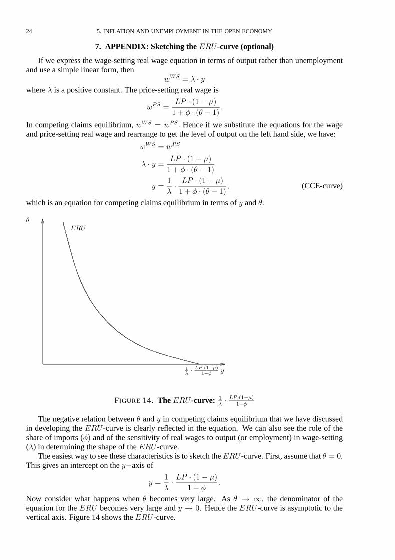
If we express the wage-setting real wage equation in terms of output rather than unemploymentand usea simple linear form, then

�� & � �

where& isa positiveconstant. Theprice-setting real wage is

��

� � � ��

In competing claims equilibrium, �� Hence if we substitute the equations for the wageand price-setting real wageand rearrange to get the level of output on the left hand side, wehave:

��

& � � ��

� � � ��

� ��

&�

��

� � � �� (CCE-curve)

which is an equation for competing claimsequilibrium in terms of � and �.

�

��

��

FIGURE 14. The�� -curve: ��

The negative relation between � and � in competing claims equilibrium that we have discussedin developing the ��-curve is clearly re�ected in the equation. We can also see the role of theshare of imports (�� and of the sensitivity of real wages to output (or employment) in wage-setting(&) in determining the shapeof the�� -curve.

Theeasiest way to seethesecharacteristicsisto sketch the�� -curve. First, assumethat � � �.This givesan intercept on the��axis of

� ��

&��

��

Now consider what happens when � becomes very large. As � � , the denominator of theequation for the�� becomes very large and � � �. Hence the��-curve is asymptotic to thevertical axis. Figure 14 shows the�� -curve.

7. APPENDIX: SKETCHING THE �� -CURVE (OPTIONAL) 25

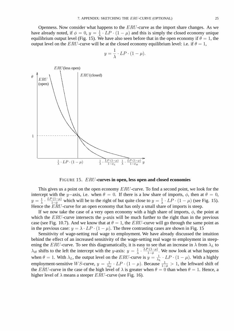
Openness. Now consider what happens to the��-curve as the import share changes. As wehave already noted, if � � �, � � �

�� and this is simply the closed economy unique

equilibrium output level (Fig. 15). We have also seen before that in the open economy if � � �, theoutput level on the��-curvewill beat theclosed economy equilibrium level: i.e. if � � �,

� ��

&� ��

�

(open)

��

��(closed)

��

��

�

�

��

�� (lessopen)

FIGURE 15. �� -curves in open, less open and closed economies

This gives us a point on the open economy �� -curve. To find a second point, we look for theintercept with the ��axis, i.e. when � � �. If there is a low share of imports, �, then at � � �,� � �

��

which will be to the right of but quite close to � � �� (see Fig. 15).

Hence the�� -curve for an open economy that has only asmall share of imports issteep.If we now take the case of a very open economy with a high share of imports, �, the point at

which the ��-curve intersects the �-axis will be much further to the right than in the previouscase (see Fig. 10.7). And we know that at � � �, the�� -curve will go through the same point asin theprevious case: � � & � �� . The threecontrasting casesareshown in Fig. 15

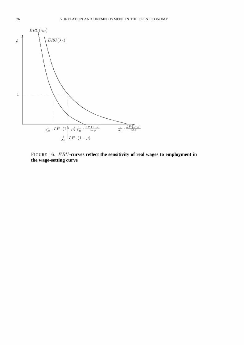
Sensitivity of wage-setting real wage to employment. We have already discussed the intuitionbehind the effect of an increased sensitivity of the wage-setting real wage to employment in steep-ening the��-curve. To see this diagramatically, it is easy to see that an increase in & from & to&� shifts to the left the intercept with the �-axis: � � �

��

� We now look at what happenswhen � � �. With & , the output level on the�� -curve is � � �

�� . With a highly

employment-sensitive -curve, � � �� Because �

�� , the leftward shift of

the��-curve in the case of the high level of & is greater when � � � than when � � �. Hence, ahigher level of & meansasteeper ��-curve (seeFig. 16).


�

��

�

��

��

��

��

��

FIGURE 16. ��-curves re�ect the sensitivity of real wages to employment inthe wage-setting curve

Documents

Ination and unemployment in the open economyuctpa36/ch5feb0303.pdf · Ination and unemployment in the open economy ... What factors inuence the rate of unemployment and output level