Incentives from Compensation and Career Movements on Work

1

Incentives from Compensation and Career Movements on Work

Performance: Evidence from a Reform of Personnel Policies

Bicheng Yang, Tat Chan, Hideo Owan, Tsuyoshi Tsuru*

Abstract

This paper empirically studies the effectiveness of compensation schemes and career

movements on worker productivity in a Japanese auto sales firm that offers its employees

both types of incentives. A salesperson’s work performance influences not only his current

commission, but also future career movements including promotion to the managerial level

or transfer to other non-sales jobs. In response to the economic recession, the firm started

a reform in personnel management that drastically revamped the compensation structure

and how salespeople are promoted or transferred, providing us with rich data variation for

estimating a dynamic model that captures salespeople’s work effort decisions under

different incentive systems. Our results show that, compared with the counterfactual

scenario when there are only monetary compensations as the reward for performance,

career movements increase the firm’s gross profit by 95 percent, suggesting that long-term

incentives can significantly complement short-term incentives to enhance employees’

productivity. The opportunity of promotion provides a much stronger incentive to

salespeople than the fear of being transferred. We also find that about half of the profit

increase from the reform comes from the increased power of the incentive from the

compensation scheme, and the rest from the change in the system of career movements.

Finally, we illustrate how the firm can implement an alternative policy for job evaluations

that places more weight on performance to further incentivize the work effort from young

and middle-aged salespeople, and how the firm can achieve a higher net profit by changing

the current wage spread between managers and salespeople.

JEL Codes: J01; J24; J30;

* Bicheng Yang ([email protected]) is an Assistant Professor of Marketing and Behavioural Science at the Sauder School of

Business, University of British Columbia. Tat Chan ([email protected]) is a Professor of Marketing at the Olin Business School,

Washington University in St. Louis. Hideo Owan ([email protected]) is a Professor of Economics at the Institute of Social Science,

University of Tokyo. Tsuyoshi Tsuru ([email protected]) is a Professor of Economics at the Institute of Economic Research, Hitotsubashi University. The authors thank Auto Japan for providing the data. They are also grateful for feedback from seminar

participants at Washington University in St. Louis, University of Toronto, University of British Columbia, University of Minnesota,

University of Colorado, University of Delaware, Cornell University, University of Rochester, Hong Kong Polytechnic University, University of Tokyo and Hitotsubashi University. All errors in this paper are ours. Corresponding author: Bicheng Yang.

mailto:[email protected]




2

1. Introduction

To motivate the work effort from employees, firms often explicitly or implicitly offer

employees a contract package including short-term incentives, in the form of a

performance-related compensation scheme, and long-term incentives that come from

potential career movements within the firm. Stimulated by a large stream of theoretical

research on the power of incentives (Lazear 2000) in personnel economics, the past two

decades witnessed a rapid growth of empirical research that identifies the relationship

between worker compensation and productivity (for examples see Paarsch and Shearer

1999, 2000; Shearer 2004; Lazear 2000; Bandiera, Barankay, and Rasul 2007; Misra and

Nair 2011; Chung, Steenburgh, and Sudhir 2014; Chan, Li and Pierce 2014). Promotion

and demotion policies, on the other hand, provide a long-term incentive as the current

performance of employees will influence future monetary and non-monetary payoffs. The

tournament theory, starting from the seminal work of Lazear and Rosen (1981), has been

used to explain why it is efficient for firms to use career advancements as an incentive.

In many cases, combining both incentives in contract offers can be mutually beneficial

for firms and employees. If an optimal compensation scheme which fully solves the moral

hazard problem is difficult to implement, career movements can be used as a complement

for the compensation to improve worker incentives. The effectiveness of the two incentives

may also vary across employees. For young employees, career advancements may be the

primary concern in their work decisions, but for employees who are near the age of

retirement, such a long-term goal may no longer be relevant and the short-term incentive

becomes more important (Gibbons and Murphy 1991). The effectiveness also depends on

how the compensation scheme and career movements are linked to work performance.

3

Knowing how each type of incentives works for different types of employees is essential

for firms to understand how to improve the incentive system.

The objective of this paper is to study the effectiveness of compensation schemes and

career movements on the worker productivity. We study a personnel dataset on car

salespeople provided by an auto sales firm in Japan, who offers employees both types of

incentives. Previous research on the incentives of compensation schemes primarily uses a

static modeling framework, as an employee’s work performance is typically rewarded by

the pay in the same period. To study career movements, however, a dynamic framework is

required. This is because promotions and demotions typically rely on the evaluations of

work performance over time, as such the incentive will primarily come from career

concerns for the long future. To achieve our objective, we develop a structural dynamic

model that allows both types of incentives to influence an employee’s current and future

work effort choices. The model also allows that, when facing a negative outcome in the

career path, the employee may leave the firm to seek outside opportunities in the external

labor market. Furthermore, we let promotions and demotions involve changes in jobs that

are differentiated in not only monetary but also non-monetary payoffs, which are related

to the difficulty of job tasks, work environment, and prestige etc. Although the focus of the

study is one particular empirical setting, this model can be applied to various compensation

and promotion and demotion systems. Using the estimation results from the structural

model, researchers can then investigate how employees will respond to alternative

counterfactual systems of incentives.

We choose the personnel data on salespeople as our empirical application for several

reasons. First, salesforce is an important component of the economy. The Bureau of Labor

4

Statistics reports that about 14 million people in the United States were employed in sales-

related occupations in 2012, more than 10% of the workforce. The amount that firms spend

on their salesforce is three times as high as spending on advertising (Zoltners et al. 2008).

Understanding how the incentives work for salespeople thus has important economic

implications. Second, for each salesperson, the data contains detailed descriptions of his

compensation including the base wage and commissions, career movements involving

changes in the job level as a salesperson, and promotion to the managerial level or transfers

to non-sales jobs (which are equivalent to demotions), over time. It also reports the gross

profit the salesperson contributes in each month which, from the firm’s perspective, is an

accurate measure of the worker productivity. This data nature enables us to investigate the

relationship between an employee’s performance and his short-term and long-term

incentives. Finally, during the data period, the firm started a reform in its personnel

management policies which drastically revamped the compensation structure and how

salespeople are promoted or transferred, hoping that it would improve the sales

performance. This policy change enhances the identification of our model, as we can use

not only the data variation across salespeople who are at different points of the career path

but also within each salesperson the change in the work performance after the reform to

identify the effectiveness of the two types of incentives.

Estimation results show that, relative to the sales job, managerial jobs bring an

employee higher monetary and non-monetary payoffs, while non-sales jobs are worse off

in both dimensions. Career concerns are important when salespeople make the work effort

decision. Compared with the counterfactual scenario when there are only monetary

compensations as the reward for performance, the system of career movements (after

5

reform) increases the firm’s gross profit by 95 percent, suggesting that long-term incentives

can significantly complement short-term incentives to enhance employees’ productivity.

The opportunity of promotion provides a much stronger incentive to salespeople than the

fear of being transferred. Furthermore, data shows that the reform of the firm was

successful in increasing the productivity of salespeople. A decomposition of the effect,

based on the estimation results, shows that about half of the profit increase has come from

the increased power of the incentive from the compensation scheme, about 40 percent from

the change in the system of promotions or transfers, and the rest from the change in how

salespeople move upward or downward within the sales job. Finally, we use the model to

illustrate how the firm can implement an alternative system of career movements that

weights more on the work performance to further incentivize the work effort from young

and middle-aged salespeople, and how the firm can achieve a higher net profit by changing

the current wage spread between managers and salespeople.

Our paper is organized as follows: Section 2 reviews the relevant literature. Section 3

describes the data and presents some data statistics and patterns. Section 4 specifies the

model and discusses the estimation strategy. Section 5 presents results from the model

estimation and policy experiments. Finally Section 6 concludes.

2. Related literature

When a worker’s effort cannot be directly measured, the problem of moral hazard arises

and understanding a worker’s incentives is key to contract design. There is a large

theoretical literature on the design of optimal contract. Under the principal-agent

framework, researchers have shown that the optimal contract should be non-linear on a

6

worker’s output (e.g. Holmstrom 1979; Lazear 1986). In the sales-force context, research

has focused on the design and implementation of compensation plan to incentivize the

optimal level of effort from salespeople (e.g. Basu et al. 1985; Coughlan and Sen 1989;

Rao 1990; Lal and Srinivasan 1993). A number of empirical studies in the economics and

marketing literature have tested the relationship between worker compensation and

productivity (e.g. Paarsch and Shearer 1999, 2000; Shearer 2004; Lazear 2000; Bandiera,

Barankay, and Rasul 2007; Coughlan and Narasimhan 1992, Lal, Outland, and Staelin

1994, Joseph and Kalwani 1998; Misra et al. 2005; Chan, Li and Pierce 2014). The setting

in these studies is static. Recently, there is a small stream of empirical works studying the

dynamic effects of the compensation scheme. For example, Misra and Nair (2011) study

how workers respond to a payment scheme with quotas and floors and ceilings for pay, and

conclude that quotas reduce productivity. Chung et al. (2014) study the compensation

scheme with quota and bonus and find that it enhances productivity. Our paper shares some

similarities with these two papers by using a dynamic structural model to back out

salespeople’s effort and estimate their utility primitives. However, we study the

salespeople’s long-term career concerns in addition to their short-term monetary incentives.

The hierarchical job structure of firms, together with the pay scheme, provides an incentive

for better work performance if workers are forward-looking.

Our paper is also related to the literature in economics on career movements within a

company. There are multiple views underlie the existence of internal career movements.

One is that for certain jobs the entry from the external job market is restricted, either by

administrative rules or because of firm-specific human capital accumulation required for

these jobs (Doeringer and Piore 1985, Becker 2009). Another view is that, as a firm owns

7

the private information regarding the ability of its workers, it will use promotions to

preserve such information advantage and thus create long careers within the firm (e.g.

Waldman 1984, Greenwald 1986). The tournament theory, starting from the seminal work

of Lazear and Rosen (1981), has also been used to explain the pattern of career

advancements within firms. In the model, workers compete for prizes the value of which

is measured by the wage difference between pre- and post-promotions. Firms use

promotions to induce the optimal level of effort from the pre-promotion job. Baker, Gibbs

and Holmstrom (1994a, 1994b) demonstrate in details the wage and job hierarchy structure

in a medium-sized U.S. firm in a service industry over 20 years and find no clear support

to the first two theories and find support to the tournament theory. The tournament theory

has also been tested by a number of other empirical studies (e.g. Lazear 1992, Audas,

Barmby, and Treble 2004, and DeVaro and Waldman 2006). Our paper is closely related

to the theory by studying the influence of promotions and demotions on salespeople’s work

incentives. Instead of testing the theory, we develop a dynamic structural model to quantify

the incentives from career movements, in addition to that from the short-term compensation.

Moreover, in addition to the wage difference following job changes, we also investigate

the difference in non-monetary benefits (or costs).

One recent paper by Gayle, Golan and Miller (2015) studies the firm-size pay gap (i.e.

large firm pays more than smaller firms) in the executive market. It develops a dynamic

structural model to investigate how an executive makes job and effort choices considering

his compensation, nonpecuniary benefits from working and future value of human capital

accumulation. Unlike our study, the work performance of executives is not observed from

data; thus, Gayle et al assume that contracts are made optimally between an agent and a

8

firm so that they can recover the effort choice of executives. Also, the focus of the paper is

the external labor market where executives move across firms. Our research focuses on the

internal market of a single firm where salespeople face a specific compensation scheme

and promotion and demotion system. Our findings are more relevant to the question of how

firms can offer a better contract package that will improve workers’ performance.

To sum up, our paper differs from the previous literature by studying an internal labor

market where the firm offers both short-term compensation and long-term career

movements as incentives for employees. We use a structural dynamic model to help

quantify the importance of these two types of incentives.

3. Data and Descriptive Analysis

3.1. Background

The firm that provides us data is one of the largest regional chain dealers in Japan, selling

and leasing cars produced by one of the largest auto manufacturers in the world. The firm

owns 74 outlets, most of which have a new car sales section, a used car sales section, and

a service section, ranged from 3 salespeople at the smallest outlet to 22 at the largest. In

2004, the firm had 2,300 employees, 1/3 of them were salespeople. Most employees are

hired at young age (the average starting age is 20.8), and retire at the age of 60. The annual

total sales in that year was $1.3 billion US Dollar.1 As a comparison, according to the report

of Automotive News on top car dealers in the US, the firm is equivalent to the 20th largest

dealer in the US as measured by total sales.

1 We convert Japanese Yen to US Dollar throughout this paper.

9

Our data period is from April 1998 to December 2005. Every month, a salesperson is

paid a base wage and a commission. Within the sales job, there are upward or downward

movements in “levels” that are tied to the change in the base wage. There are also

movements across jobs, as a salesperson may be promoted to the managerial level or

transferred to a non-sales job, such as a clerk who mainly undertakes routine administrative

duties.

In October 2000, the firm launched a reform in personnel management policies, as a

response to the economic recession during that period. The recession, which is referred to

as the “Lost 20 Years” in Japan, lasted from 1990 to 2010 during which the whole country

experienced stagnant economic growth. The firm’s car sales also suffered for a long period.

The objective of the reform is to improve salespeople’s performance. We are told by the

firm that the idea of the reform is to increase the incentive power for employees by relating

the compensation and career movements more closely with a salesperson’s performance

(Lazear 2000).

We first examine from data how the compensation scheme of salespeople changes.

Before the reform (Period 0, from April 1998 to September 2000), each month a

salesperson earns a fix base wage plus the commission from the cars he sells in that month.

The commission of a car is calculated as the gross profit, i.e., the sales revenue deducted

by the cost of the cars sold, multiplied by the commission rate of the car. The average

commission rate of all the cars sold during the period is 4.5%. After the reform (from

October 2000 to December 2005), the average commission rate significantly increases to

21.2%. The payment structure also changes, as a salesperson’s monthly pay is the

maximum of his base wage and the commission.

10

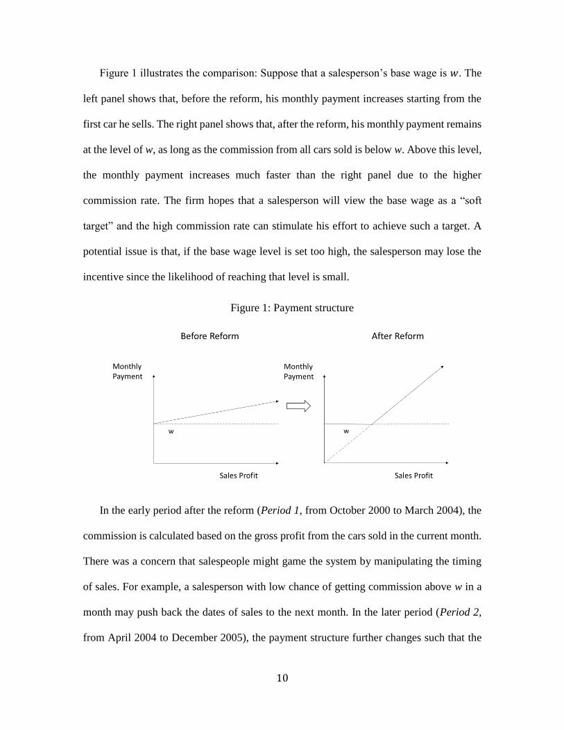
Figure 1 illustrates the comparison: Suppose that a salesperson’s base wage is 𝑤. The

left panel shows that, before the reform, his monthly payment increases starting from the

first car he sells. The right panel shows that, after the reform, his monthly payment remains

at the level of w, as long as the commission from all cars sold is below w. Above this level,

the monthly payment increases much faster than the right panel due to the higher

commission rate. The firm hopes that a salesperson will view the base wage as a “soft

target” and the high commission rate can stimulate his effort to achieve such a target. A

potential issue is that, if the base wage level is set too high, the salesperson may lose the

incentive since the likelihood of reaching that level is small.

Figure 1: Payment structure

In the early period after the reform (Period 1, from October 2000 to March 2004), the

commission is calculated based on the gross profit from the cars sold in the current month.

There was a concern that salespeople might game the system by manipulating the timing

of sales. For example, a salesperson with low chance of getting commission above w in a

month may push back the dates of sales to the next month. In the later period (Period 2,

from April 2004 to December 2005), the payment structure further changes such that the

11

commission in a month is calculated based on the salesperson’s average gross profit of the

current and the previous month. In the model which we will describe in the next section,

we take account how salespeople’s effort will change following this policy change, but we

abstract away from the potential gaming behavior which is beyond the scope of our analysis.

Regarding career movements, a salesperson’s job level may be adjusted, based on the

annual performance evaluation that is typically done by the manager of an outlet, in April

of each year. His base wage is tied to the level. The chance of being promoted to the

managerial level or transferred to a non-sales job is also influenced by the job level. The

job task does not change and a salesperson’s level is not explicitly displayed in the

workplace. To simplify our analysis, we assume that the change in the level is fully

captured by the change in the base wage, which itself will influence future promotions and

transfers.

The more significant career movements involve promotion to the managerial level or

being transferred to a non-sales job. These can happen in any month, but most are at the

beginning of April and October every year. A manager is normally the head of an outlet

and in charge of the employees of the outlet. The promotion is considered as a reward,

since the monthly payment is typically higher than that for a salesperson. Non-pecuniary

benefits may also be important because managers enjoy a more comfortable workplace and

a higher social status inside the company. Transfers to non-sales jobs, on the other hand, is

considered as a punishment to low performers, because these jobs have a lower monthly

income and status at the workplace. The job task and payment structure for managers and

non-sales jobs are completely different from those of salespeople. Salespeople may also

choose to quit the job voluntarily if their pecuniary or non-pecuniary returns are too low or

12

there is not enough opportunity for career advancement inside the firm.2 In this case, they

will seek new jobs in the external labor market and we no longer have their record.

3.2. Some summary statistics

In this study, we focus on 340 salespeople who start their job in the new car department

and exclude those who work in other departments or move to the new car department from

other departments during the data period. Our data consists of each salesperson’s monthly

sales profit, base wage, job movements, and some demographic information including the

age and education level.

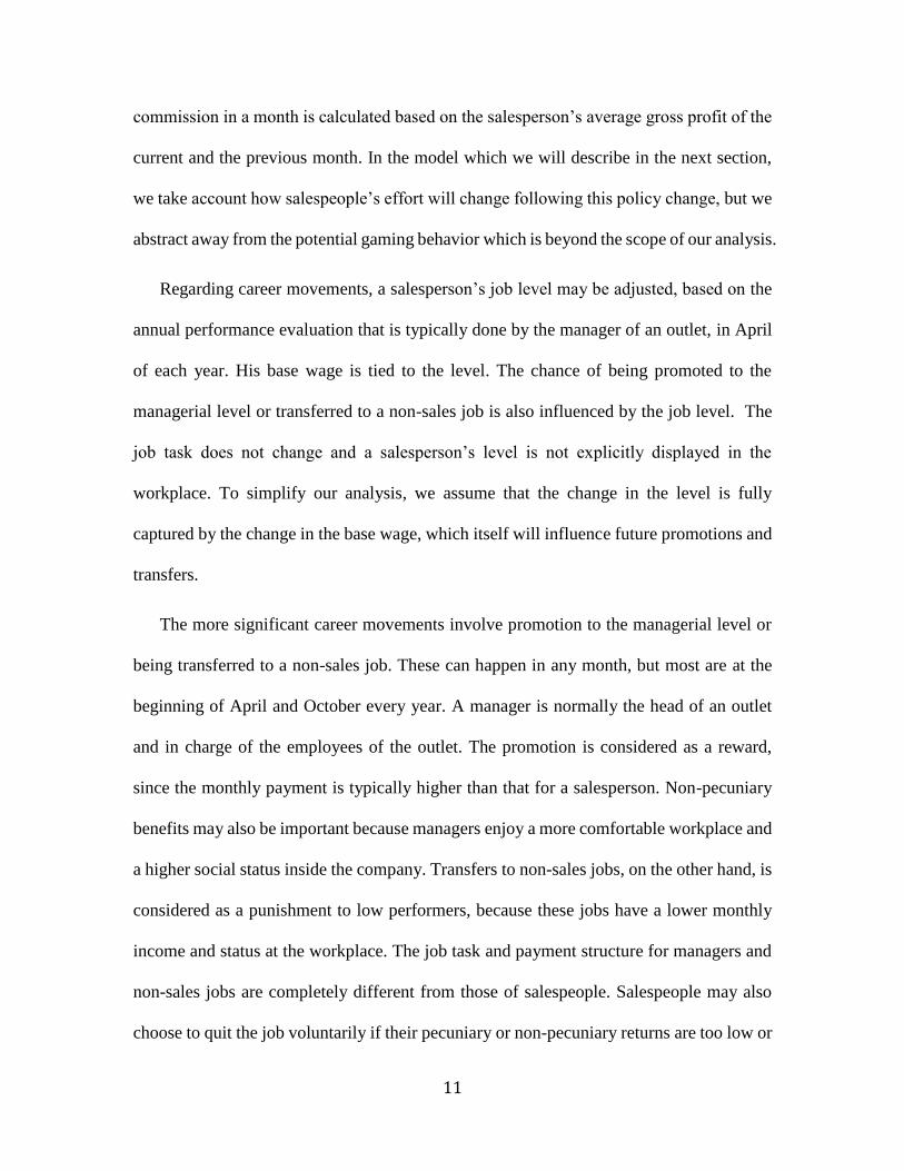
Table 1 presents the mean and standard deviation (in parentheses) of the monthly sales

profit, commission, and base wage, of each salesperson, broken down by age groups,

before and after the reform. The average sales profit after the reform has significantly

increased for all age groups and, as a result, the commission is also higher. The base wage

for young salespeople has increased, but it has been reduced for salespeople at older age.

This is because, as we will show below, the reform has changed the evaluation system to

one based more on workers’ performance and less on the seniority.

Table 1: Summary statistics for sales profit, commission and base wage

2 Layoffs are rare in Japan as most firms provide life-long job security for employees.

All Age<35 35<Age<50 50<Age<60 All Age<35 35<Age<50 50<Age<60

Monthly sales profit (1,000 USD) 11.90 11.68 12.11 11.02 15.95 18.03 16.39 13.43

(3.68) (3.68) (3.63) (3.11) (4.27) (5.44) (4.4) (3.59)

Monthly commission (1,000 USD) 0.54 0.52 0.55 0.48 3.39 3.80 3.46 2.94

(0.15) (0.15) (0.14) (0.12) (0.84) (1.06) (0.86) (0.71)

Monthly base wage (1,000 USD) 3.01 2.47 3.19 3.82 3.23 2.90 3.18 3.74

(0.1) (0.09) (0.07) (0.06) (0.07) (0.24) (0.04) (0.04)

Before reform After reform

13

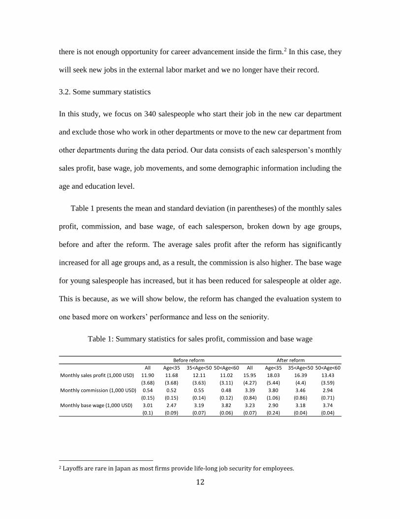
The first three rows in Table 2 compare the monthly income of salespeople, managers

and other non-sales jobs before and after the reform. The average income of managers is

the highest and that of other non-sales jobs is the lowest. The reform has increased the

income of managers and other non-sales jobs but the extent is smaller than that for the sales

job. The income of employees at different jobs can change over time. We do not have the

information on the pay scheme for and work performance of managers and other non-sales

jobs. Table 3 shows the results of regressing the monthly payment of each job on the age

and the reform indicator. Similar to what Table 2 shows, the reform increases the income

of managers and non-sales jobs. It also increases with the age at a rate faster than that for

salespeople.

The last three rows of Table 2 compare the annual rate of promotions, transfers and

voluntary quits. The likelihoods of these career movements are in general small. The rate

of promotions is about twice higher than the rate of transfers, and the rate of voluntary quits

is the smallest. Because of the improved sales profit after the reform, promotions have

significantly increased and transfers and quits have decreased.

Table 2: Summary statistics for income of different jobs and career movements


Monthly income of salespeople (1,000 USD) 3.6 4.0

Monthly income of non-sales jobs (1,000 USD) 3.2 3.4

Monthly income of managers (1,000 USD) 4.2 4.4

Annual rates of transfers 3.7% 2.2%

Annual rates of promotions 2.3% 6.9%

Annual rates of quits 2.9% 0.8%

14

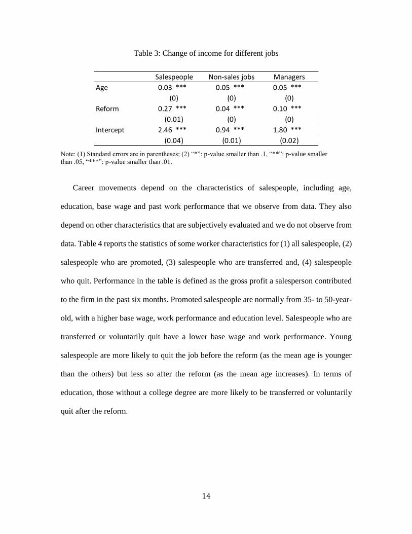
Table 3: Change of income for different jobs

Note: (1) Standard errors are in parentheses; (2) “*”: p-value smaller than .1, “**”: p-value smaller

than .05, “***”: p-value smaller than .01.

Career movements depend on the characteristics of salespeople, including age,

education, base wage and past work performance that we observe from data. They also

depend on other characteristics that are subjectively evaluated and we do not observe from

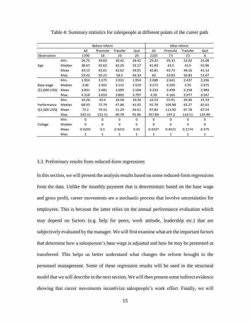
data. Table 4 reports the statistics of some worker characteristics for (1) all salespeople, (2)

salespeople who are promoted, (3) salespeople who are transferred and, (4) salespeople

who quit. Performance in the table is defined as the gross profit a salesperson contributed

to the firm in the past six months. Promoted salespeople are normally from 35- to 50-year-

old, with a higher base wage, work performance and education level. Salespeople who are

transferred or voluntarily quit have a lower base wage and work performance. Young

salespeople are more likely to quit the job before the reform (as the mean age is younger

than the others) but less so after the reform (as the mean age increases). In terms of

education, those without a college degree are more likely to be transferred or voluntarily

quit after the reform.

Age 0.03 *** 0.05 *** 0.05 ***

Reform 0.27 *** 0.04 *** 0.10 ***

Intercept 2.46 *** 0.94 *** 1.80 ***

(0)

(0.01)

(0.02)

(0)

(0)

(0)

(0)

(0.01)(0.04)

Salespeople Non-sales jobs Managers

15

Table 4: Summary statistics for salespeople at different points of the career path

3.3. Preliminary results from reduced-form regressions

In this section, we will present the analysis results based on some reduced-form regressions

from the data. Unlike the monthly payment that is deterministic based on the base wage

and gross profit, career movements are a stochastic process that involve uncertainties for

employees. This is because the latter relies on the annual performance evaluation which

may depend on factors (e.g. help for peers, work attitude, leadership etc.) that are

subjectively evaluated by the manager. We will first examine what are the important factors

that determine how a salesperson’s base wage is adjusted and how he may be promoted or

transferred. This helps us better understand what changes the reform brought to the

personnel management. Some of these regression results will be used in the structural

model that we will describe in the next section. We will then present some indirect evidence

showing that career movements incentivize salespeople’s work effort. Finally, we will

n_manager

All Promote Transfer Quit All Promote Transfer Quit

Observation 1390 16 26 20 2105 73 23 8

Min. 26.75 34.83 30.42 28.42 29.25 35.33 32.92 31.08

Age Median 38.67 43.62 42.29 33.17 41.83 43.5 43.5 41.96

Mean 39.12 43.01 42.62 34.91 42.81 43.73 44.16 41.14

Max. 59.42 50.25 58.5 46.33 60 53.83 56.83 51.67

Min. 1.954 3.175 2.031 1.954 2.089 2.641 2.437 2.296

Base wage Median 3.06 3.502 3.115 2.529 3.272 3.505 3.35 2.975

($1,000 USD) Mean 3.041 3.485 3.099 2.584 3.233 3.499 3.258 2.984

Max. 4.318 3.659 3.802 3.797 4.39 4.165 3.977 3.567

Min. 10.26 33.4 26.58 10.26 16.53 55.91 30.46 25.33

Performance Median 68.93 72.79 47.86 41.92 92.78 109.88 65.27 62.61

($1,000 USD) Mean 72.2 79.15 51.29 46.61 97.83 113.92 67.78 67.54

Max. 192.31 131.31 90.78 91.86 357.89 197.2 116.51 134.99

Min. 0 0 0 0 0 0 0 0

College Median 0 0 0 0 0 0 0 0

Mean 0.4295 0.5 0.4231 0.45 0.4337 0.4521 0.2174 0.375

Max. 1 1 1 1 1 1 1 1

After reformBefore reform

16

present evidence on how the reform has changed the work performance of workers at

different ages.

3.3.1 Change in the base wage

A salesperson’s job level is adjusted every year in April. Based on the previous discussion,

we assume the adjustment is fully captured by the change in the base wage. At the

beginning of each (annual) wage cycle 𝑏, the change in his base wage from the previous

cycle follows the following process:

Δ𝐵𝑖𝑏 = 𝑏0𝑗+ 𝑏1

𝑗∗ 𝑎𝑔𝑒𝑖𝑡 + 𝑏2

𝑗∗ 𝐵𝑖𝑏−1 + 𝑏3

𝑗∗ 𝑦𝑖𝑏−1,−𝑡 + 𝑏4

𝑗∗ 𝑒𝑑𝑢𝑖 + 𝜖𝑖𝑏

𝑗 (1)

That is, the change in base wage (Δ𝐵𝑖𝑏) depends on a salesperson’s age (𝑎𝑔𝑒𝑖𝑡), current

base wage (𝐵𝑖𝑏−1), the performance in the last year (𝑦𝑖𝑏−1,−𝑡) and education level (𝑒𝑑𝑢𝑖 =

1 if with college degree or 𝑒𝑑𝑢𝑖 = 0 if without). We do not incorporate tenure in the

regression because age and tenure are highly correlated (correlation = 0.94). In our data,

almost all of the salespeople are hired by the firm at the age of early 20s. Finally, the error

term in the regression captures the impact from other factors that are subjectively evaluated

by the manager and we as researchers do not observe.

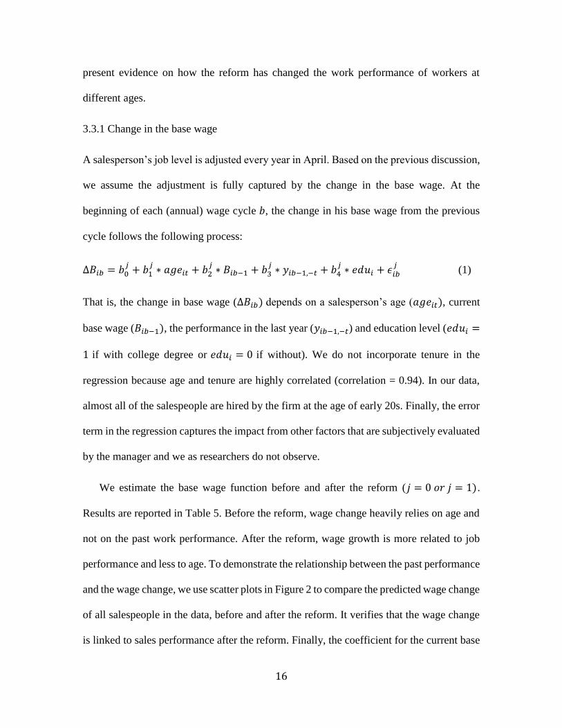
We estimate the base wage function before and after the reform (𝑗 = 0 𝑜𝑟 𝑗 = 1).

Results are reported in Table 5. Before the reform, wage change heavily relies on age and

not on the past work performance. After the reform, wage growth is more related to job

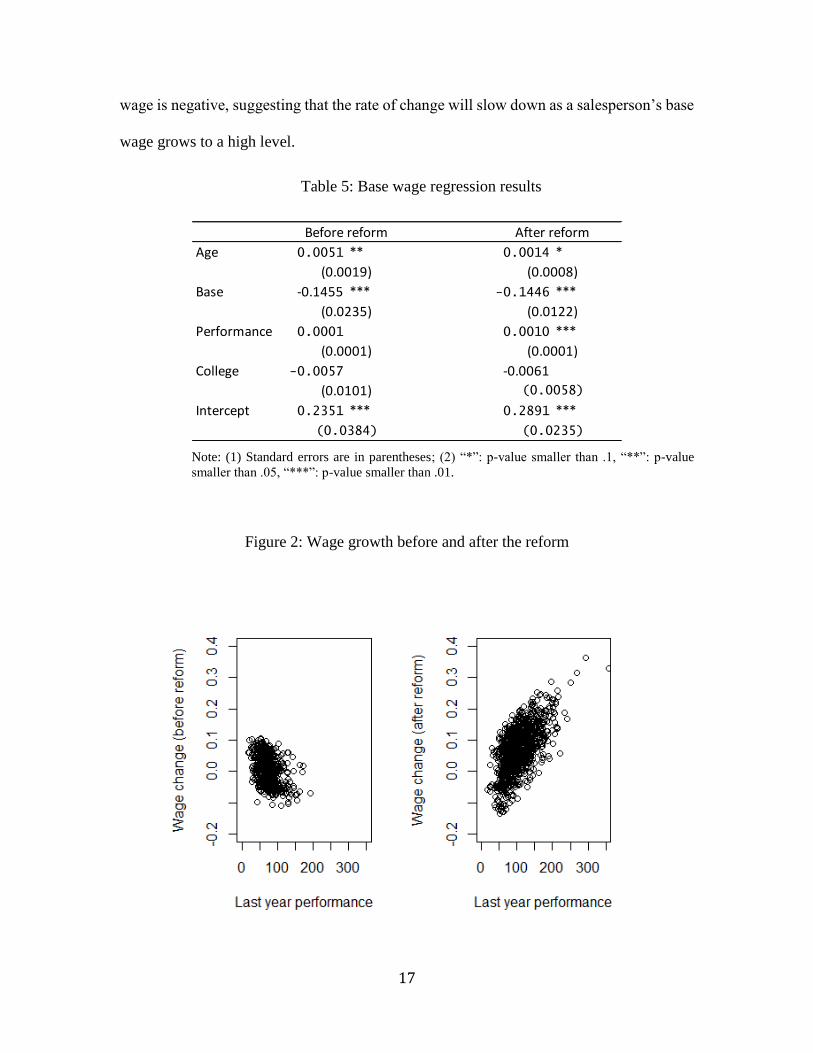
performance and less to age. To demonstrate the relationship between the past performance

and the wage change, we use scatter plots in Figure 2 to compare the predicted wage change

of all salespeople in the data, before and after the reform. It verifies that the wage change

is linked to sales performance after the reform. Finally, the coefficient for the current base

17

wage is negative, suggesting that the rate of change will slow down as a salesperson’s base

wage grows to a high level.

Table 5: Base wage regression results

Note: (1) Standard errors are in parentheses; (2) “*”: p-value smaller than .1, “**”: p-value

smaller than .05, “***”: p-value smaller than .01.

Figure 2: Wage growth before and after the reform

Age 0.0051 ** 0.0014 *

Base -0.1455 *** -0.1446 ***

Performance 0.0001 0.0010 ***

College -0.0057 -0.0061

Intercept 0.2351 *** 0.2891 ***

(0.0101) (0.0058)

(0.0235)(0.0384)


(0.0019)

(0.0235)

(0.0001)

(0.0008)

(0.0122)

(0.0001)

18

3.3.2 Career movements

Promotions and transfers usually happen at the beginning of April and October every year.

For simplicity, we assume that all the career movements happen between April and October

are determined in April, and all those happen between October and the next April are

determined in October. We use an ordered probit regression to represent the career

movement system. That is, at the beginning of the first month 𝑡 (i.e. April or October) of

each (half-yearly) career movement cycle 𝑚 , the performance evaluation 𝑀𝑖𝑚 for

salesperson 𝑖 is determined by:

𝑀𝑖𝑚 = 𝑚1 ∗ 𝑎𝑔𝑒𝑖𝑡 + 𝑚2 ∗ 𝑎𝑔𝑒𝑖𝑡2 + 𝑚3 ∗ 𝑒𝑑𝑢𝑖 + 𝑚4

𝑗∗ 𝐵𝑖𝑏𝑡 + 𝑚5

𝑗∗ 𝑦𝑖𝑚−1,−𝑡 + 𝜖𝑖𝑚

𝑗 (2)

And the probability of promotion ( 𝑃(𝑃𝑖𝑚𝑡 = 1) ) and that of transfer ( 𝑃(𝐿𝑖𝑚𝑡 = 1)

conditional on the salesperson’s evaluation are

𝑃(𝑃𝑖𝑚𝑡 = 1) = 𝑃(𝑀𝑖𝑚 > 𝑢𝑝) (3)

and

𝑃(𝐿𝑖𝑚𝑡 = 1) = 𝑃(𝑀𝑖𝑚 < 𝑢𝐿) (4)

where 𝜖𝑖𝑚~𝑁(0,1) captures the impact of the subjective evaluations that are unobserved

to us as researchers. The variable 𝑦𝑖𝑚−1,−𝑡 represents the salesperson’s performance in the

past six months. We assume that the salesperson will be promoted (i.e. 𝑃𝑖𝑚𝑡 = 1 ) if his

evaluation is above a threshold (i.e. 𝑀𝑖𝑚 > 𝑢𝑝), or he will be transferred (i.e. 𝐿𝑖𝑚𝑡 = 1 )

if the evaluation is below another threshold (i.e. 𝑀𝑖𝑚 < 𝑢𝑙). If the evaluation is in between,

i.e. 𝑢𝑝 ≤ 𝑀𝑖𝑚 ≤ 𝑢𝑙, the salesperson will stay as a salesperson (i.e. 𝑆𝑖𝑚𝑡 = 1). Note that in

equation (2) the evaluation is a function of the base wage 𝐵𝑖𝑏𝑡. Therefore, the adjustment

19

in the salesperson’s job level will change not only his monthly income but also his chance

of being promoted or transferred.

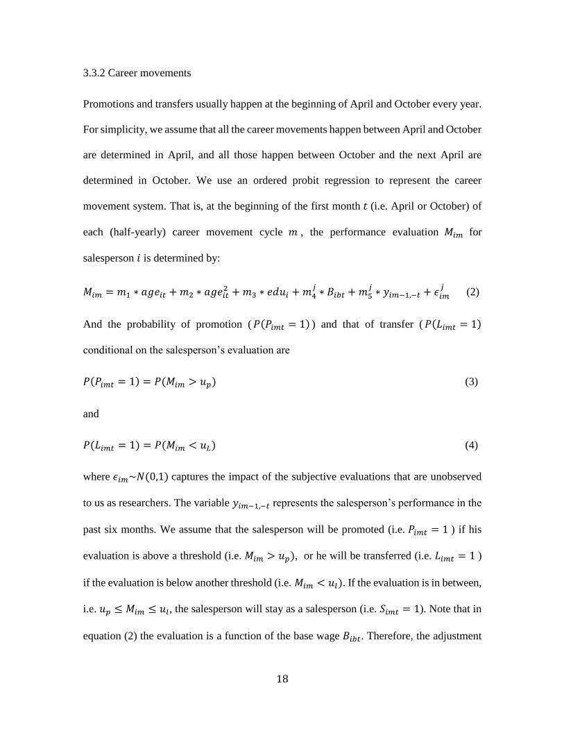
Table 6: Regression results for promotions and transfers

Note: (1) Standard errors are in parentheses; (2) “*”: p-value smaller than .1,

“**”: p-value smaller than .05, “***”: p-value smaller than .01.

Since we do not have many observations of career movements, estimating separate

regressions for before and after the reform will be inefficient. Therefore, we assume that

the two thresholds (𝑢𝑝 and 𝑢𝐿 ) and the coefficients for age, 𝑎𝑔𝑒2 and 𝑒𝑑𝑢𝑖 remain

unchanged, but allow the coefficients for 𝐵𝑖𝑏𝑡 and 𝑦𝑖𝑚−1,−𝑡 to be different before and after

the reform. Table 6 reports the regression results. Age has an inverted U-shaped

relationship with the performance evaluation, suggesting that salespeople at middle age are

more likely to be promoted and young and old salespeople are more likely to be transferred.

Salespeople with a college degree and better job performances are also more likely to be

Base_before 0.3562 **

Performance_before 0.0104 ***

Base_after 0.5636 ***

Performance_after 0.0044 ***

Age 0.1488 **

Age2 -0.0019 **

College 0.1387 *

Threshold: transfer 2.5400 *

Threshold: promote 6.9690 ***

(0.0765)

(1.301)

(1.322)

(0.1575)

(0.1558)

(0.0026)

(0.0016)

(0.0648)

(0.0007)

20

promoted and less likely to be transferred. The smaller coefficient for the past performance

after the reform is mainly due to the overall higher sales profit. The coefficient for the base

wage has increased and, as Table 5 shows, the change in the base wage becomes more

related to the past performance. Combining with this indirect effect, past performance is a

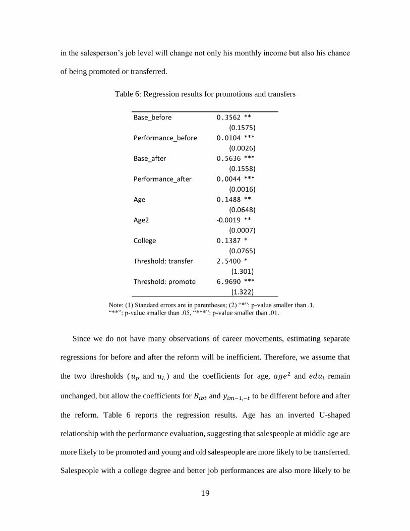
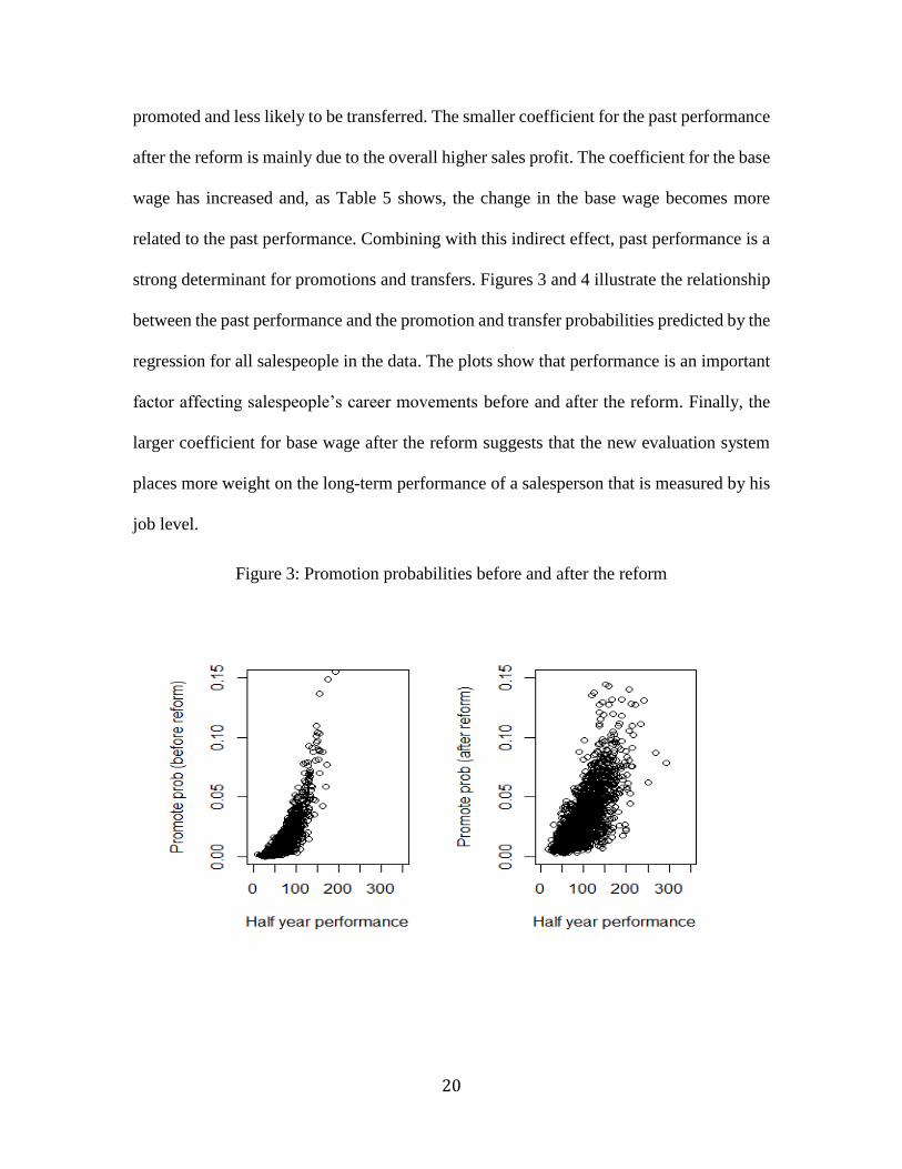
strong determinant for promotions and transfers. Figures 3 and 4 illustrate the relationship

between the past performance and the promotion and transfer probabilities predicted by the

regression for all salespeople in the data. The plots show that performance is an important

factor affecting salespeople’s career movements before and after the reform. Finally, the

larger coefficient for base wage after the reform suggests that the new evaluation system

places more weight on the long-term performance of a salesperson that is measured by his

job level.

Figure 3: Promotion probabilities before and after the reform

21

Figure 4: Transfer probabilities before and after the reform

3.3.3. The response to career movements

The relationship between pay schemes and workers’ productivity has been documented in

previous empirical studies (e.g. Paarsch and Shearer 1999, 2000; Shearer 2004; Lazear

2000; Bandiera, Barankay, and Rasul 2007). To find evidence from data that career concern

is an important factor for workers’ effort, however, is more challenging. This is because

career movements are a long process that is based on the work performance over many

periods. Our strategy is to investigate whether a salesperson’s performance increases when

the probability of promotion or transfer is high, after controlling for other factors. The

rationale is that, assuming the salesperson discounts the payoffs from the long future more

than the near future, he will invest more work effort to facilitate the promotion or to avoid

being transferred, as long as these events have a significant impact on the welfare.

22

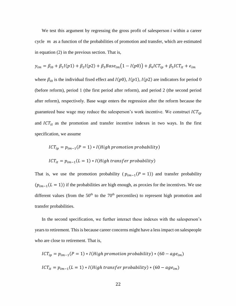
We test this argument by regressing the gross profit of salesperson 𝑖 within a career

cycle 𝑚 as a function of the probabilities of promotion and transfer, which are estimated

in equation (2) in the previous section. That is,

𝑦𝑖𝑚 = 𝛽𝑖0 + 𝛽1𝐼(𝑝1) + 𝛽2𝐼(𝑝2) + 𝛽3𝐵𝑎𝑠𝑒𝑖𝑚(1 − 𝐼(𝑝0)) + 𝛽4𝐼𝐶𝑇𝑖𝑝 + 𝛽5𝐼𝐶𝑇𝑖𝑡 + 𝜖𝑖𝑚

where 𝛽𝑖0 is the individual fixed effect and 𝐼(𝑝0), 𝐼(𝑝1), 𝐼(𝑝2) are indicators for period 0

(before reform), period 1 (the first period after reform), and period 2 (the second period

after reform), respectively. Base wage enters the regression after the reform because the

guaranteed base wage may reduce the salesperson’s work incentive. We construct 𝐼𝐶𝑇𝑖𝑝

and 𝐼𝐶𝑇𝑖𝑡 as the promotion and transfer incentive indexes in two ways. In the first

specification, we assume

𝐼𝐶𝑇𝑖𝑝 = 𝑝𝑖𝑚−1(𝑃 = 1) ∗ 𝐼(𝐻𝑖𝑔ℎ 𝑝𝑟𝑜𝑚𝑜𝑡𝑖𝑜𝑛 𝑝𝑟𝑜𝑏𝑎𝑏𝑖𝑙𝑖𝑡𝑦)

𝐼𝐶𝑇𝑖𝑡 = 𝑝𝑖𝑚−1(𝐿 = 1) ∗ 𝐼(𝐻𝑖𝑔ℎ 𝑡𝑟𝑎𝑛𝑠𝑓𝑒𝑟 𝑝𝑟𝑜𝑏𝑎𝑏𝑖𝑙𝑖𝑡𝑦)

That is, we use the promotion probability ( 𝑝𝑖𝑚−1(𝑃 = 1)) and transfer probability

(𝑝𝑖𝑚−1(𝐿 = 1)) if the probabilities are high enough, as proxies for the incentives. We use

different values (from the 50th to the 70th percentiles) to represent high promotion and

transfer probabilities.

In the second specification, we further interact these indexes with the salesperson’s

years to retirement. This is because career concerns might have a less impact on salespeople

who are close to retirement. That is,

𝐼𝐶𝑇𝑖𝑝 = 𝑝𝑖𝑚−1(𝑃 = 1) ∗ 𝐼(𝐻𝑖𝑔ℎ 𝑝𝑟𝑜𝑚𝑜𝑡𝑖𝑜𝑛 𝑝𝑟𝑜𝑏𝑎𝑏𝑖𝑙𝑖𝑡𝑦) ∗ (60 − 𝑎𝑔𝑒𝑖𝑚)

𝐼𝐶𝑇𝑖𝑡 = 𝑝𝑖𝑚−1(𝐿 = 1) ∗ 𝐼(𝐻𝑖𝑔ℎ 𝑡𝑟𝑎𝑛𝑠𝑓𝑒𝑟 𝑝𝑟𝑜𝑏𝑎𝑏𝑖𝑙𝑖𝑡𝑦) ∗ (60 − 𝑎𝑔𝑒𝑖𝑚)

23

where (60 − 𝑎𝑔𝑒𝑖𝑚) represents the number of years before retirement.

Table 7: Regression results: performance and career concerns

Specification (1)

Specification (2)



The results of the regressions are reported in Table 7. The coefficients for 𝐼𝐶𝑇𝑖𝑡 are

significantly positive under all specifications, suggesting that, when facing a higher chance

of being transferred, a salesperson will work hard to prevent the transfer. The coefficients

for 𝐼𝐶𝑇𝑖𝑝 are also positive, however, only the estimates in the second specification are

significant. This implies that the near-future promotion only has a strong effect for younger

salespeople.

Thresholds (percentile)

Base*(1-Period 0) -8.7737 *** -8.8799 *** -9.0694 ***

ICTp 35.9720 35.3602 20.6750

ICTt 165.6848 *** 137.6978 *** 146.8585 ***

Period 1 57.1987 *** 57.1947 *** 58.1696 ***

Period 2 50.5786 *** 50.5817 *** 51.6200 ***

Fix effects

50% 60% 70%

Individual

(2.1672)

(25.4583)

(39.4015)

(6.8823)

(7.181)

Individual

(2.1633)

(24.1218)

(36.7939)

(6.8915)

(7.1839)

Individual

(2.1922)

(28.4864)

(44.0452)

(6.9682)

(7.2621)

Thresholds (percentile)

Base*(1-Period 0) -8.853 *** -8.9922 *** -9.3578 ***

ICTp 2.2876 2.6745 ** 2.0991 *

ICTt 4.7014 ** 3.7335 ** 4.2514 ***

Period 1 56.6619 *** 56.7032 *** 58.2411 ***

Period 2 49.9595 *** 49.9358 *** 51.5494 ***

Fix effects

50% 60% 70%

(7.4654) (7.4098) (7.4301)

Individual Individual Individual

(1.8659) (1.6976) (1.5804)

(7.1217) (7.0672) (7.1007)

(2.2092) (2.1949) (2.2029)

(1.4397) (1.315) (1.2506)

24

Note that the above results do not fully capture the effect of promotions or transfers on

workers’ performance. Rather, they only show how salespeople respond to an increased

likelihood of promotion or transfer by adjusting their effort, as an indirect evidence that

career concerns do impact their performance. The true effect of promotions and transfers

should be higher than the results here. For example, even though the likelihood of

promotion or transfer is small for a young salesperson who is just hired by the firm, future

career advancements can still be a strong motivation for him to work hard. Such an effect

cannot be captured by the reduced-form regression and can only be quantified using a

structural modeling approach, which we will discuss in detail in the next section.

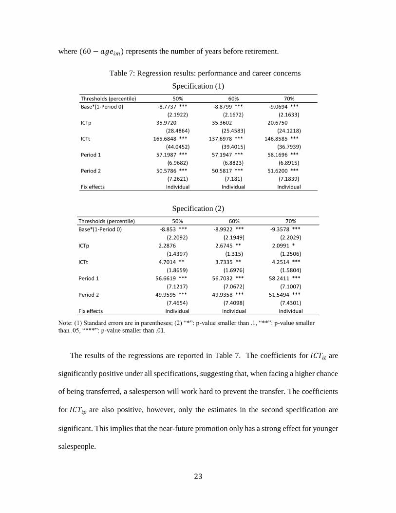
3.3.4. Effectiveness of the reform

Next, we investigate whether the reform is effective and what is its impact on different

types of salespeople. We use another regression that specifies the sales profit of salesperson

𝑖 in month 𝑡 as

𝑦𝑖𝑡 = 𝛽0𝑖 + 𝛽1𝑖𝐼(𝑝1) + 𝛽2𝑖𝐼(𝑝2) + 𝛽3𝑆𝑒𝑎𝑠𝑜𝑛𝑎𝑙𝑖𝑡𝑦𝑡 + 𝜖𝑖𝑡

where 𝛽0𝑖 is an individual fixed effect, and 𝐼(𝑝1), 𝐼(𝑝2) are indicators for the two periods

after the reform. 𝑆𝑒𝑎𝑠𝑜𝑛𝑎𝑙𝑖𝑡𝑦𝑡 captures the impact of seasonality on the market demand.

We construct this index using the aggregate sales in the region where the firm locates in

each month from 1999 to 2004, and calculate 𝑆𝑒𝑎𝑠𝑜𝑛𝑎𝑙𝑖𝑡𝑦𝑡 as 𝑆𝑎𝑙𝑒𝑠 𝑜𝑓 𝑚𝑜𝑛𝑡ℎ 𝑡

𝑆𝑎𝑙𝑒𝑠 𝑜𝑓 𝑀𝑎𝑟𝑐ℎ.3 We run

four regressions: the first two regressions assume 𝛽0𝑖 to be the same across salespeople,

while the next two estimate the individual fixed effect. The first and the third regression

assume that 𝛽1𝑖 and 𝛽2𝑖 are the same across salespeople. In the second and the last

3 We use the sales in March as the baseline because its sales are the highest.

25

regression, we allow that 𝛽1𝑖 and 𝛽2𝑖 are different for salespeople who are younger than 35,

between 35 and 50, and older than 50, to investigate whether the reform has different

effects on salespeople with different ages.

Table 8: Reduced-form regressions: the effectiveness of the reform



Results in Table 8 show that the reform is overall effective in improving salespeople’s

performance, and the effect is robust under different specifications. Another robust finding

is that the effect is the strongest for young salespeople. This finding can have several

explanations. First, it may be that older salespeople overall have higher base wages, so it

is less likely that their sales commission can exceed their base wage. This may reduce the

effect of the reform for older salespeople. Second, since young salespeople are further away

from retirement, they may care more about future career movements. For older salespeople,

Period 1 5.1783 *** 5.0767 ***

Period 2 3.1028 *** 3.5168 ***

Period 1:20-35 6.6203 *** 5.5938 ***

Period 1:35-50 5.6097 *** 5.4266 ***

Period 1:50-60 3.2182 *** 3.1136 ***

Period 2:20-35 5.1102 *** 4.3765 ***

Period 2:35-50 3.9601 *** 4.2480 ***

Period 2:50-60 1.7140 *** 1.3744 ***

Seasonality 23.1784 *** 23.1654 *** 23.1626 *** 23.1899 ***

Fix effects

(0.5664)

(0.4426) (0.4394)

No Group

(0.5809)

(0.591)

(0.2301)

Regression 1 Regression 2

(0.1534)

(0.3478)

(0.22)

(0.1482)

Regression 3 Regression 4

Individual Individual

(0.3153)

(0.2015)

(0.4086)

(0.5873)

(0.2218)

(0.3586)

(0.3929)

(0.1399)

(0.15)

(0.3935)

26

however, promotions are less likely and thus are less relevant. As career movements are

more related to job performance after the reform, the effect is thus stronger for young

salespeople. It is impossible to separate these two effects from reduced-form regressions.

Instead, our structural model will allow us to better understand how the reform influence

the incentives of salespeople.

4. Model

Based on the institutional details of the firm and the data patterns we observe, we build a

dynamic model of salesforce response to wage changes and career movements. The

sequence of decisions in the model are as follows:

1. At the beginning of a career movement cycle m (April for the cycle between April and

September, and October for the cycle between October and the next March) of a year,

salesperson i decides whether to quit or not by comparing his expected utility of

staying and quitting. Conditional on the salesperson stays, the firm decides whether to

promote or to transfer the salesperson.

2. Conditional on the salesperson stays (not quit, promoted or transferred), at the

beginning of a wage cycle b (every April) of a year, the firm decides the salesperson’s

base wage of this cycle.

3. Conditional on the worker remains at the sales job, at the beginning of a month t, a

salesperson observes all his current states and exerts selling effort in a dynamically

optimal manner. An idiosyncratic sales shock, which is known by the salesperson up

to the distribution, is realized.

4. Conditional on the salesperson stays, step 1-3 repeat until the salesperson retire at age

60.

27

4.1 Sales response function and salesperson per period utility

We model salesperson 𝑖’s work performance in month 𝑡, which is measured by his monthly

gross sales profit (𝑦𝑖𝑡), as a function of his effort 𝑒𝑖𝑡

𝑦𝑖𝑡 = 𝑆𝑒𝑎𝑠𝑜𝑛𝑎𝑙𝑖𝑡𝑦𝑡 ∗ 𝑒𝑖𝑡 + 𝜖𝑖𝑡 (5)

where 𝑆𝑒𝑎𝑠𝑜𝑛𝑎𝑙𝑖𝑡𝑦𝑡 is the seasonality index we construct from regional sales data, as

discussed in 3.3.4. It can be treated as a proxy of market potential, and when exerting the

same level of effort, a salesperson’s sales profit is on average higher when the market

potential is larger. 𝜖𝑖𝑡 is a stochastic component of sales profit that is assumed to be

distributed as 𝑁(0, 𝜎𝑗2).

Putting effort in selling cars is costly to a salesperson. The cost function is specified as

the following:

𝑐𝑖𝑡 =1

2𝛽𝑖𝑒𝑖𝑡

2 (6)

where 𝛽𝑖 is restricted to be positive; that is, cost is a convex-increasing function of effort.

Since effort is unobservable, a strictly monotonic parametric relationship between sales

and effort is necessary for identification purposes. The individual-specific parameter 𝛽𝑖 is

a function of salesperson’s demographics (age and education level).

Let j denote the period before the reform (0), first period (1), or second period (2), after

the reform. Salesperson 𝑖’s utility in month 𝑡, 𝑈𝑖𝑡𝑗, is his monetary income 𝑤𝑖𝑡

𝑗 minus his

selling effort 𝑐𝑖𝑡, which is

𝑈𝑖𝑡𝑗

= 𝑤𝑖𝑡𝑗− 𝑐𝑖𝑡 (7)

28

The monetary income is calculated differently for different period 𝑗 due to the reform.

More specifically, before the reform (𝑗 = 0),

𝑤𝑖𝑡0 = 𝐵𝑖𝑏 + 𝑟0𝑦𝑖𝑡 (8)

First period after the reform (𝑗 = 1),

𝑤𝑖𝑡1 = max (𝐵𝑖𝑏, 𝑟1𝑦𝑖𝑡) (9)

Second period after the reform (𝑗 = 2),

𝑤𝑖𝑡2 = max (𝐵𝑖𝑏, 𝑟2

(𝑦𝑖𝑡+𝑦𝑖𝑡−1)

2) (10)

where 𝐵𝑖𝑏 is salesperson 𝑖’s base wage in wage cycle 𝑏,𝑟0, 𝑟1 and 𝑟2 are commission rates

of the three periods, where 𝑟1 = 𝑟2.

4.2 Salesperson utility from career movements

As discussed in Section 3, we use linear regression and ordered probit regression to

represent the wage growths and career movements. That is, salesperson 𝑖’s wage change

from previous wage cycle, Δ𝐵𝑖𝑏 , is determined as in equation (1), and promotion and

transfer are based on the evaluation measurement, 𝑀𝑖𝑚, which is determined by equation

(2), and the probabilities that a salesperson is promoted and transferred are (9) and (10).

For simplicity, we further assume that once promoted or transferred, the salesperson

stays as a manager or in another department until retirement. Let 𝑛𝑖𝑡 denote the month left

from month 𝑡 to the salesperson’s retirement (at age 60). The value of promotion at month

𝑡 is the discounted value of the stream of utility as a manager in all future months until

retirement, which is specified as the following:

𝑉𝑖𝑚𝑡𝑝 = Σ𝑘=1

𝑛𝑖𝑡 𝛿𝑘−1 ∗ (𝑤𝑖,𝑡+𝑘−1𝑝 + 𝑢𝑖,𝑡+𝑘−1

𝑝 ) (11)

29

where 𝛿 is the monthly discount rate (fixed at 0.98); 𝑤𝑖,𝑡+𝑘−1𝑝

is the monetary payoff as a

manager that is approximated using the regression results in Table 3; 𝑢𝑖,𝑡+𝑘−1𝑝

is the non-

monetary utility of a manager that is a function of the manager’s demographics (age and

education level) that is estimated from the data. Note that ex-ante, 𝑢𝑝 can be either positive

or negative as it is the difference between the non-monetary benefits of a manager, e.g.

better work environment and prestige, and his effort cost assuming that the manager put in

the optimal effort in each month, conditional on the incentive system after promotion.

Similarly, the value associated with lateral transfer is specified as

𝑉𝑖𝑚𝑡𝐿 = Σ𝑘=1

𝑛𝑖𝑡 𝛿𝑘−1 ∗ (𝑤𝑖,𝑡+𝑘−1𝐿 + 𝑢𝑖,𝑡+𝑘−1

𝐿 ) (12)

where 𝑤𝑖,𝑡+𝑘−1𝐿 is the monetary payoff after transfer that is approximated using the

regression results in Table 3; 𝑢𝑖,𝑡+𝑘−1𝐿 is the non-monetary utility after transfer that is a

function of salesperson’s demographics and is estimated from the data, assuming that the

worker put in the optimal effort in each month, conditional on the incentive system after

transfer.

Besides being promoted or transferred, a salesperson can also quit the job. Different

from promotions and transfers which are decisions of the firm, whether to quit the company

is a voluntary decision of a salesperson. Though a salesperson can quit at any time, we

assume that a salesperson only considers whether to quit at the beginning of a career

movement cycle before 𝑃 or 𝐿 is realized. We make this simplified assumption as we only

observe 28 quits and it is infeasible for us to identify the reason for quitting in different

months. If the salesperson quits, he will not return to the company. The value of quitting is

specified as

30

𝑉𝑖𝑚𝑡𝑄 = Σ𝑘=1

𝑛𝑖𝑡 𝛿𝑘−1 ∗ 𝑢𝑖,𝑡+𝑘−1𝑄 + 𝜖𝑖𝑚𝑡

𝑄 (13)

where 𝑢𝑖,𝑡+𝑘−1𝑄

is the expected utility (includes both monetary and non-monetary utilities)

from an outside job at period 𝑡 + 𝑘 − 1. We again allow 𝑢𝑖,𝑡+𝑘−1𝑄

to be a function of

salesperson’s demographics. In addition, 𝜖𝑖𝑚𝑡𝑄 ~(0, 𝜎𝑞

2) is a one-time shock that rationalizes

the stochastic decision to quit.

4.3 Life-time value and optimal decisions

Follow our previous discussions, the key state variables (𝑋𝑖𝑡) evolve as follows:

1. Age

𝐴𝑔𝑒𝑖𝑡 = 𝐴𝑔𝑒𝑖𝑡−1 +1

12

2. Month

𝑍𝑖𝑡 = {𝑍𝑖𝑡−1 + 1, 𝑖𝑓 𝑍𝑖𝑡−1 < 121, 𝑖𝑓 𝑍𝑖𝑡−1 = 12

3. Base wage

𝐵𝑖𝑏𝑡 = {𝐵𝑖𝑏−1𝑡−1 + Δ𝐵𝑖𝑏, 𝑖𝑓 𝑍𝑖𝑡 = 4𝐵𝑖𝑏𝑡−1, 𝑜𝑡ℎ𝑒𝑟𝑤𝑖𝑠𝑒

4. Accumulated sales within this wage cycle

𝑦𝑖𝑏,−𝑡 = {0, 𝑖𝑓 𝑍𝑖𝑡 = 4

𝑦𝑖𝑏,−(𝑡−1) + 𝑦𝑖𝑡−1, 𝑜𝑡ℎ𝑒𝑟𝑤𝑖𝑠𝑒

5. Accumulated sales within this career movement cycle

𝑦𝑖𝑚,−𝑡 = {0, 𝑖𝑓 𝑍𝑖𝑡 = 4 𝑜𝑟 𝑍𝑖𝑡 = 10 𝑦𝑖𝑚,−(𝑡−1) + 𝑦𝑖𝑡−1, 𝑜𝑡ℎ𝑒𝑟𝑤𝑖𝑠𝑒

6. Sales of last period: 𝑦𝑖𝑡−1

31

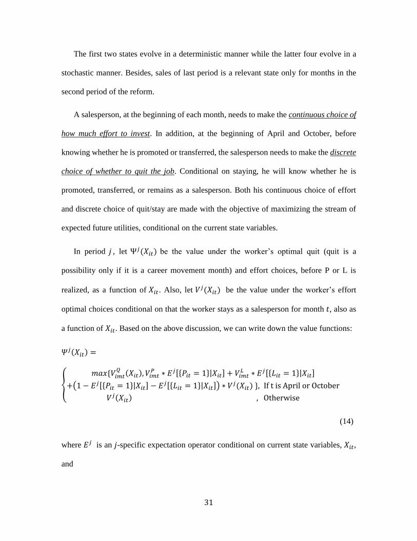
The first two states evolve in a deterministic manner while the latter four evolve in a

stochastic manner. Besides, sales of last period is a relevant state only for months in the

second period of the reform.

A salesperson, at the beginning of each month, needs to make the continuous choice of

how much effort to invest. In addition, at the beginning of April and October, before

knowing whether he is promoted or transferred, the salesperson needs to make the discrete

choice of whether to quit the job. Conditional on staying, he will know whether he is

promoted, transferred, or remains as a salesperson. Both his continuous choice of effort

and discrete choice of quit/stay are made with the objective of maximizing the stream of

expected future utilities, conditional on the current state variables.

In period 𝑗 , let Ψ𝑗(𝑋𝑖𝑡) be the value under the worker’s optimal quit (quit is a

possibility only if it is a career movement month) and effort choices, before P or L is

realized, as a function of 𝑋𝑖𝑡. Also, let 𝑉𝑗(𝑋𝑖𝑡) be the value under the worker’s effort

optimal choices conditional on that the worker stays as a salesperson for month 𝑡, also as

a function of 𝑋𝑖𝑡. Based on the above discussion, we can write down the value functions:

𝛹𝑗(𝑋𝑖𝑡) =

{

𝑚𝑎𝑥 {𝑉𝑖𝑚𝑡𝑄 (𝑋𝑖𝑡), 𝑉𝑖𝑚𝑡

𝑃 ∗ 𝐸𝑗[{𝑃𝑖𝑡 = 1}|𝑋𝑖𝑡] + 𝑉𝑖𝑚𝑡𝐿 ∗ 𝐸𝑗[{𝐿𝑖𝑡 = 1}|𝑋𝑖𝑡]

+(1 − 𝐸𝑗[{𝑃𝑖𝑡 = 1}|𝑋𝑖𝑡] − 𝐸𝑗[{𝐿𝑖𝑡 = 1}|𝑋𝑖𝑡]) ∗ 𝑉𝑗(𝑋𝑖𝑡) }, If t is April or October

𝑉𝑗(𝑋𝑖𝑡) , Otherwise

(14)

where 𝐸𝑗 is an 𝑗-specific expectation operator conditional on current state variables, 𝑋𝑖𝑡,

and

32

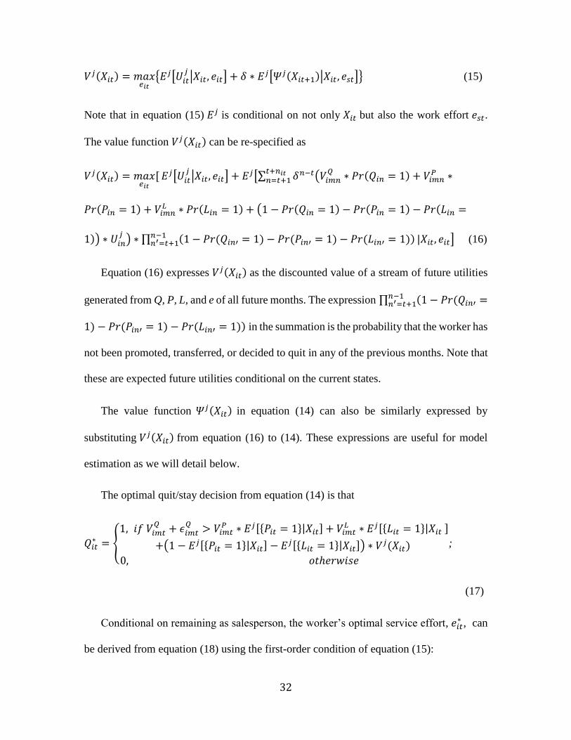
𝑉𝑗(𝑋𝑖𝑡) = 𝑚𝑎𝑥𝑒𝑖𝑡

{𝐸𝑗[𝑈𝑖𝑡𝑗|𝑋𝑖𝑡, 𝑒𝑖𝑡] + 𝛿 ∗ 𝐸𝑗[𝛹𝑗(𝑋𝑖𝑡+1)|𝑋𝑖𝑡, 𝑒𝑠𝑡]} (15)

Note that in equation (15) 𝐸𝑗 is conditional on not only 𝑋𝑖𝑡 but also the work effort 𝑒𝑠𝑡.

The value function 𝑉𝑗(𝑋𝑖𝑡) can be re-specified as

𝑉𝑗(𝑋𝑖𝑡) = 𝑚𝑎𝑥𝑒𝑖𝑡

[ 𝐸𝑗[𝑈𝑖𝑡𝑗|𝑋𝑖𝑡, 𝑒𝑖𝑡] + 𝐸𝑗[∑ 𝛿𝑛−𝑡(𝑉𝑖𝑚𝑛

𝑄 ∗ 𝑃𝑟(𝑄𝑖𝑛 = 1) + 𝑉𝑖𝑚𝑛𝑃 ∗

𝑡+𝑛𝑖𝑡𝑛=𝑡+1

𝑃𝑟(𝑃𝑖𝑛 = 1) + 𝑉𝑖𝑚𝑛𝐿 ∗ 𝑃𝑟(𝐿𝑖𝑛 = 1) + (1 − 𝑃𝑟(𝑄𝑖𝑛 = 1) − 𝑃𝑟(𝑃𝑖𝑛 = 1) − 𝑃𝑟(𝐿𝑖𝑛 =

1)) ∗ 𝑈𝑖𝑛𝑗) ∗ ∏ (1 − 𝑃𝑟(𝑄𝑖𝑛′ = 1) − 𝑃𝑟(𝑃𝑖𝑛′ = 1) − 𝑃𝑟(𝐿𝑖𝑛′ = 1))𝑛−1

𝑛′=𝑡+1 |𝑋𝑖𝑡, 𝑒𝑖𝑡] (16)

Equation (16) expresses 𝑉𝑗(𝑋𝑖𝑡) as the discounted value of a stream of future utilities

generated from Q, P, L, and e of all future months. The expression ∏ (1 − 𝑃𝑟(𝑄𝑖𝑛′ =𝑛−1𝑛′=𝑡+1

1) − 𝑃𝑟(𝑃𝑖𝑛′ = 1) − 𝑃𝑟(𝐿𝑖𝑛′ = 1)) in the summation is the probability that the worker has

not been promoted, transferred, or decided to quit in any of the previous months. Note that

these are expected future utilities conditional on the current states.

The value function 𝛹𝑗(𝑋𝑖𝑡) in equation (14) can also be similarly expressed by

substituting 𝑉𝑗(𝑋𝑖𝑡) from equation (16) to (14). These expressions are useful for model

estimation as we will detail below.

The optimal quit/stay decision from equation (14) is that

𝑄𝑖𝑡∗ = {

1, 𝑖𝑓 𝑉𝑖𝑚𝑡𝑄 + 𝜖𝑖𝑚𝑡

𝑄 > 𝑉𝑖𝑚𝑡𝑃 ∗ 𝐸𝑗[{𝑃𝑖𝑡 = 1}|𝑋𝑖𝑡] + 𝑉𝑖𝑚𝑡

𝐿 ∗ 𝐸𝑗[{𝐿𝑖𝑡 = 1}|𝑋𝑖𝑡 ]

+(1 − 𝐸𝑗[{𝑃𝑖𝑡 = 1}|𝑋𝑖𝑡] − 𝐸𝑗[{𝐿𝑖𝑡 = 1}|𝑋𝑖𝑡]) ∗ 𝑉𝑗(𝑋𝑖𝑡)

0, 𝑜𝑡ℎ𝑒𝑟𝑤𝑖𝑠𝑒

;

(17)

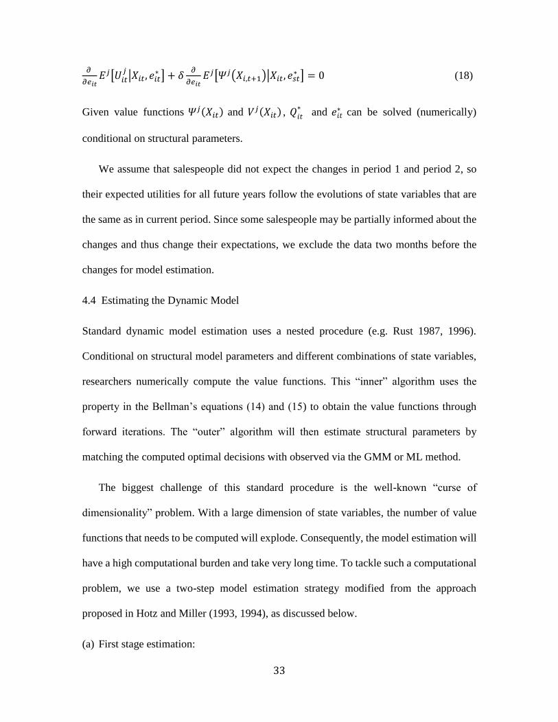
Conditional on remaining as salesperson, the worker’s optimal service effort, 𝑒𝑖𝑡∗ , can

be derived from equation (18) using the first-order condition of equation (15):

33

𝜕

𝜕𝑒𝑖𝑡𝐸𝑗[𝑈𝑖𝑡

𝑗|𝑋𝑖𝑡, 𝑒𝑖𝑡

∗ ] + 𝛿𝜕

𝜕𝑒𝑖𝑡𝐸𝑗[𝛹𝑗(𝑋𝑖,𝑡+1)|𝑋𝑖𝑡, 𝑒𝑠𝑡

∗ ] = 0 (18)

Given value functions 𝛹𝑗(𝑋𝑖𝑡) and 𝑉𝑗(𝑋𝑖𝑡) , 𝑄𝑖𝑡∗ and 𝑒𝑖𝑡

∗ can be solved (numerically)

conditional on structural parameters.

We assume that salespeople did not expect the changes in period 1 and period 2, so

their expected utilities for all future years follow the evolutions of state variables that are

the same as in current period. Since some salespeople may be partially informed about the

changes and thus change their expectations, we exclude the data two months before the

changes for model estimation.

4.4 Estimating the Dynamic Model

Standard dynamic model estimation uses a nested procedure (e.g. Rust 1987, 1996).

Conditional on structural model parameters and different combinations of state variables,

researchers numerically compute the value functions. This “inner” algorithm uses the

property in the Bellman’s equations (14) and (15) to obtain the value functions through

forward iterations. The “outer” algorithm will then estimate structural parameters by

matching the computed optimal decisions with observed via the GMM or ML method.

The biggest challenge of this standard procedure is the well-known “curse of

dimensionality” problem. With a large dimension of state variables, the number of value

functions that needs to be computed will explode. Consequently, the model estimation will

have a high computational burden and take very long time. To tackle such a computational

problem, we use a two-step model estimation strategy modified from the approach

proposed in Hotz and Miller (1993, 1994), as discussed below.

(a) First stage estimation:

34

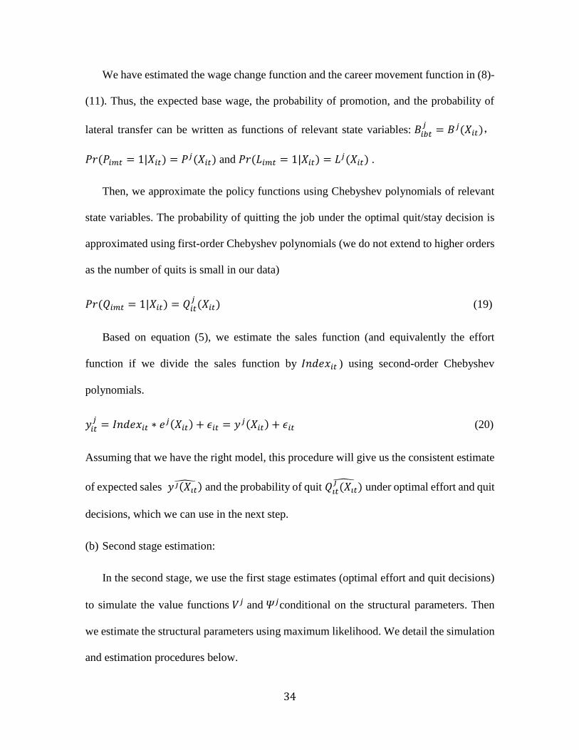
We have estimated the wage change function and the career movement function in (8)-

(11). Thus, the expected base wage, the probability of promotion, and the probability of

lateral transfer can be written as functions of relevant state variables: 𝐵𝑖𝑏𝑡𝑗

= 𝐵𝑗(𝑋𝑖𝑡)，

𝑃𝑟(𝑃𝑖𝑚𝑡 = 1|𝑋𝑖𝑡) = 𝑃𝑗(𝑋𝑖𝑡) and 𝑃𝑟(𝐿𝑖𝑚𝑡 = 1|𝑋𝑖𝑡) = 𝐿𝑗(𝑋𝑖𝑡) .

Then, we approximate the policy functions using Chebyshev polynomials of relevant

state variables. The probability of quitting the job under the optimal quit/stay decision is

approximated using first-order Chebyshev polynomials (we do not extend to higher orders

as the number of quits is small in our data)

𝑃𝑟(𝑄𝑖𝑚𝑡 = 1|𝑋𝑖𝑡) = 𝑄𝑖𝑡𝑗(𝑋𝑖𝑡) (19)

Based on equation (5), we estimate the sales function (and equivalently the effort

function if we divide the sales function by 𝐼𝑛𝑑𝑒𝑥𝑖𝑡 ) using second-order Chebyshev

polynomials.

𝑦𝑖𝑡𝑗

= 𝐼𝑛𝑑𝑒𝑥𝑖𝑡 ∗ 𝑒𝑗(𝑋𝑖𝑡) + 𝜖𝑖𝑡 = 𝑦𝑗(𝑋𝑖𝑡) + 𝜖𝑖𝑡 (20)

Assuming that we have the right model, this procedure will give us the consistent estimate

of expected sales 𝑦𝑗(𝑋𝑖𝑡) and the probability of quit 𝑄𝑖𝑡𝑗(𝑋𝑖𝑡)

under optimal effort and quit

decisions, which we can use in the next step.

(b) Second stage estimation:

In the second stage, we use the first stage estimates (optimal effort and quit decisions)

to simulate the value functions 𝑉𝑗 and 𝛹𝑗conditional on the structural parameters. Then

we estimate the structural parameters using maximum likelihood. We detail the simulation

and estimation procedures below.

35

Since a salesperson makes two type of decisions, we will search for the structural

parameters to justify the two types of observations in the data:

1. Whether a salesperson quits or stays at the beginning of each career movement cycle

given his current states.

2. Conditional on staying as a salesperson, a salesperson’s monthly sales profit given his

current states.

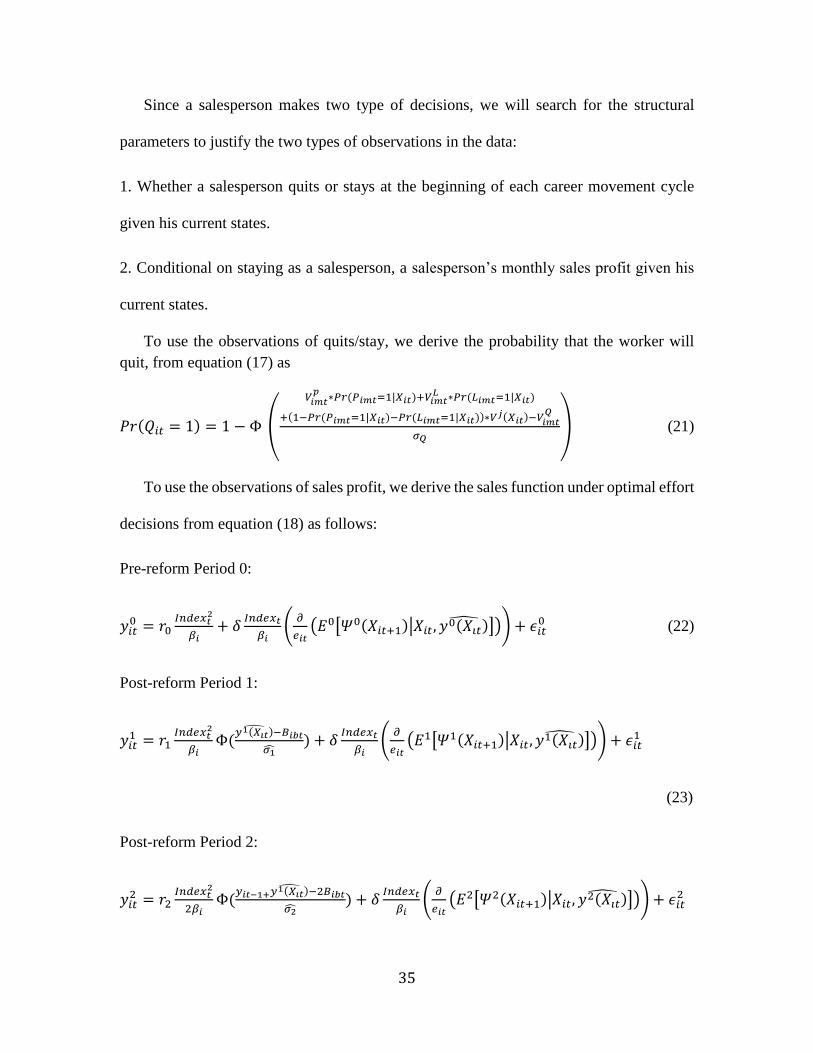
To use the observations of quits/stay, we derive the probability that the worker will

quit, from equation (17) as

𝑃𝑟(𝑄𝑖𝑡 = 1) = 1 − Φ (

𝑉𝑖𝑚𝑡𝑝

∗𝑃𝑟(𝑃𝑖𝑚𝑡=1|𝑋𝑖𝑡)+𝑉𝑖𝑚𝑡𝐿 ∗𝑃𝑟(𝐿𝑖𝑚𝑡=1|𝑋𝑖𝑡)

+(1−𝑃𝑟(𝑃𝑖𝑚𝑡=1|𝑋𝑖𝑡)−𝑃𝑟(𝐿𝑖𝑚𝑡=1|𝑋𝑖𝑡))∗𝑉𝑗(𝑋𝑖𝑡)−𝑉𝑖𝑚𝑡

𝑄

𝜎𝑄) (21)

To use the observations of sales profit, we derive the sales function under optimal effort

decisions from equation (18) as follows:

Pre-reform Period 0:

𝑦𝑖𝑡0 = 𝑟0

𝐼𝑛𝑑𝑒𝑥𝑡2

𝛽𝑖+ 𝛿

𝐼𝑛𝑑𝑒𝑥𝑡

𝛽𝑖(

𝜕

𝑒𝑖𝑡(𝐸0[𝛹0(𝑋𝑖𝑡+1)|𝑋𝑖𝑡, 𝑦0(𝑋𝑖𝑡) ])) + 𝜖𝑖𝑡

0 (22)

Post-reform Period 1:



𝛽𝑖Φ(

𝑦1(𝑋𝑖𝑡) −𝐵𝑖𝑏𝑡

𝜎1) + 𝛿


𝛽𝑖(

𝜕


1

(23)

Post-reform Period 2:



2𝛽𝑖Φ(

𝑦𝑖𝑡−1+𝑦1(𝑋𝑖𝑡) −2𝐵𝑖𝑏𝑡

𝜎2) + 𝛿


𝛽𝑖(

𝜕


2

36

(24)

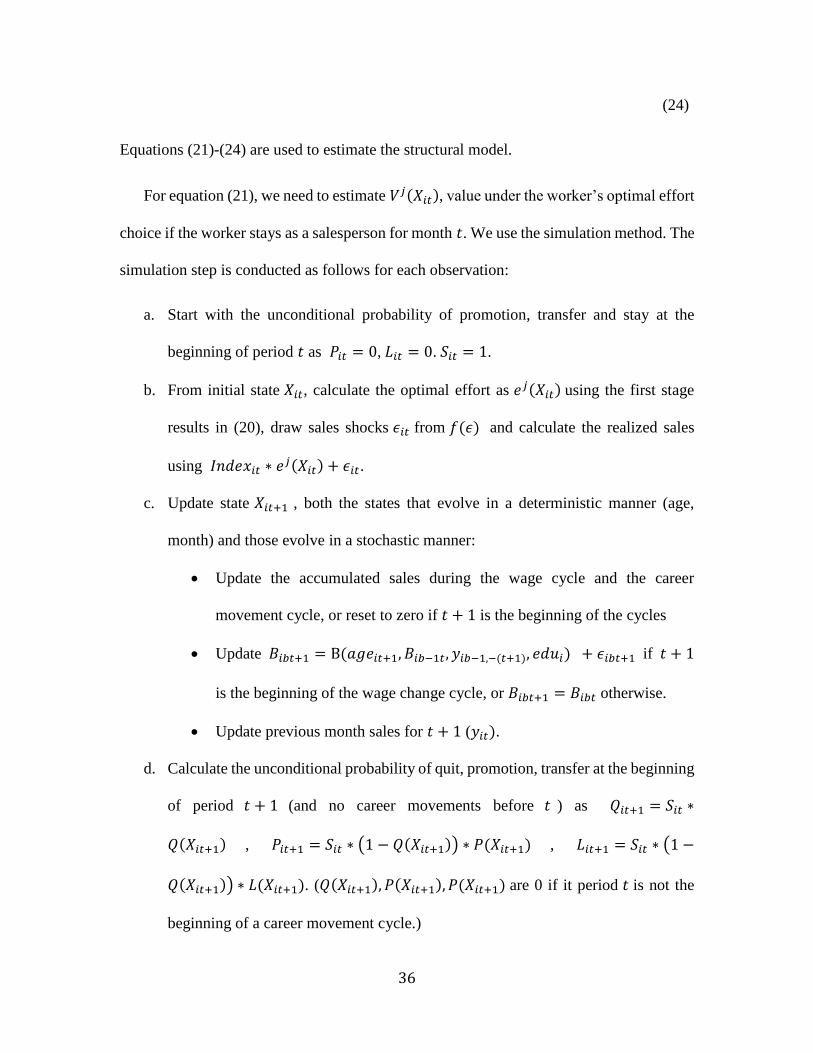
Equations (21)-(24) are used to estimate the structural model.

For equation (21), we need to estimate 𝑉𝑗(𝑋𝑖𝑡), value under the worker’s optimal effort

choice if the worker stays as a salesperson for month 𝑡. We use the simulation method. The

simulation step is conducted as follows for each observation:

a. Start with the unconditional probability of promotion, transfer and stay at the

beginning of period 𝑡 as 𝑃𝑖𝑡 = 0, 𝐿𝑖𝑡 = 0. 𝑆𝑖𝑡 = 1.

b. From initial state 𝑋𝑖𝑡, calculate the optimal effort as 𝑒𝑗(𝑋𝑖𝑡) using the first stage

results in (20), draw sales shocks 𝜖𝑖𝑡 from 𝑓(𝜖) and calculate the realized sales

using 𝐼𝑛𝑑𝑒𝑥𝑖𝑡 ∗ 𝑒𝑗(𝑋𝑖𝑡) + 𝜖𝑖𝑡.

c. Update state 𝑋𝑖𝑡+1 , both the states that evolve in a deterministic manner (age,

month) and those evolve in a stochastic manner:

Update the accumulated sales during the wage cycle and the career

movement cycle, or reset to zero if 𝑡 + 1 is the beginning of the cycles

Update 𝐵𝑖𝑏𝑡+1 = B(𝑎𝑔𝑒𝑖𝑡+1, 𝐵𝑖𝑏−1𝑡, 𝑦𝑖𝑏−1,−(𝑡+1), 𝑒𝑑𝑢𝑖) + 𝜖𝑖𝑏𝑡+1 if 𝑡 + 1

is the beginning of the wage change cycle, or 𝐵𝑖𝑏𝑡+1 = 𝐵𝑖𝑏𝑡 otherwise.

Update previous month sales for 𝑡 + 1 (𝑦𝑖𝑡).

d. Calculate the unconditional probability of quit, promotion, transfer at the beginning

of period 𝑡 + 1 (and no career movements before 𝑡 ) as 𝑄𝑖𝑡+1 = 𝑆𝑖𝑡 ∗

𝑄(𝑋𝑖𝑡+1) , 𝑃𝑖𝑡+1 = 𝑆𝑖𝑡 ∗ (1 − 𝑄(𝑋𝑖𝑡+1)) ∗ 𝑃(𝑋𝑖𝑡+1) , 𝐿𝑖𝑡+1 = 𝑆𝑖𝑡 ∗ (1 −

𝑄(𝑋𝑖𝑡+1)) ∗ 𝐿(𝑋𝑖𝑡+1). (𝑄(𝑋𝑖𝑡+1), 𝑃(𝑋𝑖𝑡+1), 𝑃(𝑋𝑖𝑡+1) are 0 if it period 𝑡 is not the

beginning of a career movement cycle.)

37

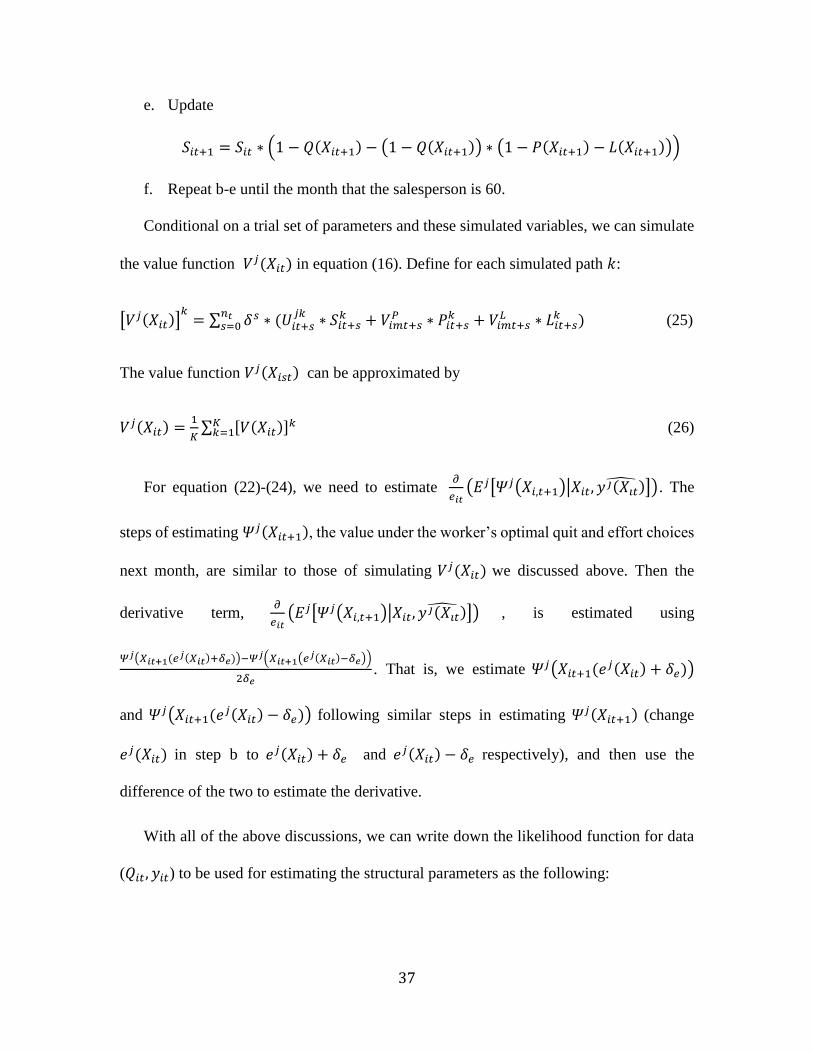
e. Update

𝑆𝑖𝑡+1 = 𝑆𝑖𝑡 ∗ (1 − 𝑄(𝑋𝑖𝑡+1) − (1 − 𝑄(𝑋𝑖𝑡+1)) ∗ (1 − 𝑃(𝑋𝑖𝑡+1) − 𝐿(𝑋𝑖𝑡+1)))

f. Repeat b-e until the month that the salesperson is 60.

Conditional on a trial set of parameters and these simulated variables, we can simulate

the value function 𝑉𝑗(𝑋𝑖𝑡) in equation (16). Define for each simulated path 𝑘:

[𝑉𝑗(𝑋𝑖𝑡)]𝑘

= ∑ 𝛿𝑠 ∗ (𝑈𝑖𝑡+𝑠𝑗𝑘

∗ 𝑆𝑖𝑡+𝑠𝑘 + 𝑉𝑖𝑚𝑡+𝑠

𝑃 ∗ 𝑃𝑖𝑡+𝑠𝑘 + 𝑉𝑖𝑚𝑡+𝑠

𝐿 ∗ 𝐿𝑖𝑡+𝑠𝑘 )

𝑛𝑡𝑠=0 (25)

The value function 𝑉𝑗(𝑋𝑖𝑠𝑡) can be approximated by

𝑉𝑗(𝑋𝑖𝑡) =1

𝐾∑ [𝑉(𝑋𝑖𝑡)]

𝑘𝐾𝑘=1 (26)

For equation (22)-(24), we need to estimate 𝜕

𝑒𝑖𝑡(𝐸𝑗[𝛹𝑗(𝑋𝑖,𝑡+1)|𝑋𝑖𝑡, 𝑦𝑗(𝑋𝑖𝑡) ]). The

steps of estimating 𝛹𝑗(𝑋𝑖𝑡+1), the value under the worker’s optimal quit and effort choices

next month, are similar to those of simulating 𝑉𝑗(𝑋𝑖𝑡) we discussed above. Then the

derivative term, 𝜕

𝑒𝑖𝑡(𝐸𝑗[𝛹𝑗(𝑋𝑖,𝑡+1)|𝑋𝑖𝑡, 𝑦𝑗(𝑋𝑖𝑡) ]) , is estimated using

𝛹𝑗(𝑋𝑖𝑡+1(𝑒𝑗(𝑋𝑖𝑡)+𝛿𝑒))−𝛹𝑗(𝑋𝑖𝑡+1(𝑒𝑗(𝑋𝑖𝑡)−𝛿𝑒))

2𝛿𝑒. That is, we estimate 𝛹𝑗(𝑋𝑖𝑡+1(𝑒

𝑗(𝑋𝑖𝑡) + 𝛿𝑒))

and 𝛹𝑗(𝑋𝑖𝑡+1(𝑒𝑗(𝑋𝑖𝑡) − 𝛿𝑒)) following similar steps in estimating 𝛹𝑗(𝑋𝑖𝑡+1) (change

𝑒𝑗(𝑋𝑖𝑡) in step b to 𝑒𝑗(𝑋𝑖𝑡) + 𝛿𝑒 and 𝑒𝑗(𝑋𝑖𝑡) − 𝛿𝑒 respectively), and then use the

difference of the two to estimate the derivative.

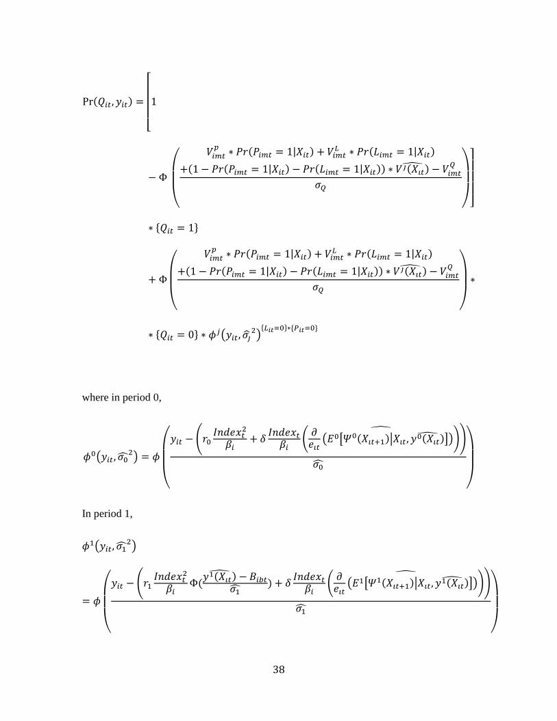
With all of the above discussions, we can write down the likelihood function for data

(𝑄𝑖𝑡, 𝑦𝑖𝑡) to be used for estimating the structural parameters as the following:

38

Pr(𝑄𝑖𝑡, 𝑦𝑖𝑡) =

[

1

− Φ

(

𝑉𝑖𝑚𝑡𝑝 ∗ 𝑃𝑟(𝑃𝑖𝑚𝑡 = 1|𝑋𝑖𝑡) + 𝑉𝑖𝑚𝑡

𝐿 ∗ 𝑃𝑟(𝐿𝑖𝑚𝑡 = 1|𝑋𝑖𝑡)

+(1 − 𝑃𝑟(𝑃𝑖𝑚𝑡 = 1|𝑋𝑖𝑡) − 𝑃𝑟(𝐿𝑖𝑚𝑡 = 1|𝑋𝑖𝑡)) ∗ 𝑉𝑗(𝑋𝑖𝑡) − 𝑉𝑖𝑚𝑡𝑄

𝜎𝑄

)

]

∗ {𝑄𝑖𝑡 = 1}

+ Φ

(

𝑉𝑖𝑚𝑡𝑝 ∗ 𝑃𝑟(𝑃𝑖𝑚𝑡 = 1|𝑋𝑖𝑡) + 𝑉𝑖𝑚𝑡

𝐿 ∗ 𝑃𝑟(𝐿𝑖𝑚𝑡 = 1|𝑋𝑖𝑡)

+(1 − 𝑃𝑟(𝑃𝑖𝑚𝑡 = 1|𝑋𝑖𝑡) − 𝑃𝑟(𝐿𝑖𝑚𝑡 = 1|𝑋𝑖𝑡)) ∗ 𝑉𝑗(𝑋𝑖𝑡) − 𝑉𝑖𝑚𝑡𝑄

𝜎𝑄

)

∗

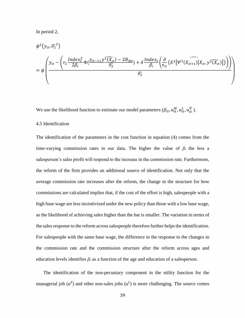
∗ {𝑄𝑖𝑡 = 0} ∗ 𝜙𝑗(𝑦𝑖𝑡, 𝜎��2)

{𝐿𝑖𝑡=0}∗{𝑃𝑖𝑡=0}

where in period 0,

𝜙0(𝑦𝑖𝑡, 𝜎02) = 𝜙

(

𝑦𝑖𝑡 − (𝑟0𝐼𝑛𝑑𝑒𝑥𝑡

2

𝛽𝑖+ 𝛿


𝛽𝑖(

𝜕𝑒𝑖𝑡

(𝐸0[𝛹0(𝑋𝑖𝑡+1)|𝑋𝑖𝑡, 𝑦0(𝑋𝑖𝑡) ])

))

𝜎0

)

In period 1,

𝜙1(𝑦𝑖𝑡, 𝜎12)

= 𝜙

(


2

𝛽𝑖Φ(

𝑦1(𝑋𝑖𝑡) − 𝐵𝑖𝑏𝑡

𝜎1) + 𝛿


𝛽𝑖(

𝜕𝑒𝑖𝑡


))

𝜎1

)

39

In period 2,

𝜙2(𝑦𝑖𝑡, 𝜎22)

= 𝜙

(


2

2𝛽𝑖Φ(

𝑦𝑖𝑡−1+𝑦1(𝑋𝑖𝑡) − 2𝐵𝑖𝑏𝑡

𝜎2) + 𝛿


𝛽𝑖(

𝜕𝑒𝑖𝑡


))

𝜎2

)

We use the likelihood function to estimate our model parameters (𝛽𝑖𝑡, 𝑢𝑖𝑡𝑀, 𝑢𝑖𝑡

𝐿 , 𝑢𝑖𝑡𝑄 ).

4.5 Identification

The identification of the parameters in the cost function in equation (4) comes from the

time-varying commission rates in our data. The higher the value of βi the less a

salesperson’s sales profit will respond to the increase in the commission rate. Furthermore,

the reform of the firm provides an additional source of identification. Not only that the

average commission rate increases after the reform, the change in the structure for how

commissions are calculated implies that, if the cost of the effort is high, salespeople with a

high base wage are less incentivized under the new policy than those with a low base wage,

as the likelihood of achieving sales higher than the bar is smaller. The variation in terms of

the sales response to the reform across salespeople therefore further helps the identification.

For salespeople with the same base wage, the difference in the response to the changes in

the commission rate and the commission structure after the reform across ages and

education levels identifies βi as a function of the age and education of a salesperson.

The identification of the non-pecuniary component in the utility function for the

managerial job (uP) and other non-sales jobs (uL) is more challenging. The source comes

40

from how salespeople respond to career movements; however, promotions and transfers in

our data are a long process that is based on the work performance over many periods. A

key identification assumption we rely on is that salespeople use the same career movement

function, before and after the reform, that we estimate from equation (2) to form the

expectation for promotion and transfer. With this assumption, the utility parameters are

identified from two types of data variation. The first is within each individual how the sales

performance changes as he approaches different points in the career path. Suppose a

salesperson’s performance improves as the likelihoods of promotion and transfer increases,

to an extent larger than what can be explained by the pre- and post-promotion or transfer

wage difference. This suggests that he is working harder to enhance the opportunity of

promotion or avoid being transferred, implying a positive (negative) non-pecuniary

component in uP (uL). Second, as we discussed in the data section, the reform changes the

career movement policy from one based on seniority to another weighted more on the

performance (through how performance impacts the evolution of the base wage which will

then impact promotions and transfers). Before and after the reform comparison also

enhances the identification. For example, suppose after the reform young salespeople

increase sales profit more than their older counterparts, to an extent that cannot be

explained by the change in the compensation scheme. Our model will infer that young

salespeople are responding to the higher promotion opportunity and therefore the utility for

the managerial job is higher than that for the sales job. For salespeople with the same

likelihoods of promotion and transfer, the difference in their responses across ages and

education levels identifies uP and uL as a function of the age and education of a salesperson.

41

Finally, after uL is identified, the quit rate among salespeople will identify the utility

function of quit (uQ). If the quit rate is low even for those who are very close to being

transferred, this implies the utility after quitting is more negative than the utility for other

non-sales jobs. In addition, the variation of the quit rates among salespeople with different

likelihoods of being transferred helps identify the standard deviation of the error term 𝜖𝑄

in equation (13). If the standard deviation is large, the variation of quit rates will be small.

5 Estimation Results and Counterfactuals

In this section, we first present the results from estimating the dynamic structural model

described in the previous section. We also compare with two alternative models to

illustrate how the proposed model improves the in-sample data fit. Next, we use the

estimation results to quantify the impact of the career movement policy currently adopted

by the firm on the worker performance. We then investigate the underlying factors that

contribute to the effectiveness of the reform. Finally, we propose alternative career

movement policies that further change either how performance is evaluated or the payment

for promoted and transferred employees. We show how these policies can be implemented

by the firm to further improve its profit.

5.1. Estimation results

To investigate the importance of incorporating workers’ career concerns in our proposed

model, we also estimate two alternative models. The first model is static, assuming that a

salesperson is myopic and thus he does not consider future career movements when making

the effort decision. He decides whether to quit by comparing his expected utility of staying

with the firm with the utility of leaving in the current month. This setting is equivalent to

fixing the discount factor to zero in the proposed model. The second model, a dynamic

42

model without promotions and transfers, assumes that the salesperson considers how his

current effort influences the future change in the base wage for the sales job. However, he

does not consider the chance of promotion or transfer. This setting is equivalent to fixing

the probabilities of promotions and transfers to zero in the proposed model.

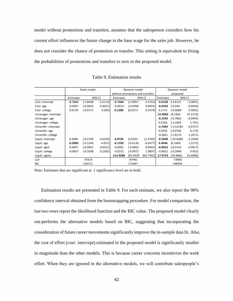
Table 9. Estimation results

Note: Estimates that are significant at .1 significance level are in bold.

Estimation results are presented in Table 9. For each estimate, we also report the 90%

confidence interval obtained from the bootstrapping procedure. For model comparison, the

last two rows report the likelihood function and the BIC value. The proposed model clearly

out-performs the alternative models based on BIC, suggesting that incorporating the

consideration of future career movements significantly improve the in-sample data fit. Also,

the cost of effort (cost: intercept) estimated in the proposed model is significantly smaller

in magnitude than the other models. This is because career concerns incentivize the work

effort. When they are ignored in the alternative models, we will contribute salespeople’s

Estimates Estimates Estimates

Cost: intercept -5.7241 [-5.8448 -5.6113] -5.7344 [-5.9957 -5.3755] -4.0128 [-4.8131 -3.0001]

Cost: age -0.0007 [-0.0033 0.0021] -0.0013 [-0.0096 0.0042] -0.0259 [-0.044 -0.0058]

Cost: college 0.0178 [-0.0171 0.049] 0.1280 [0.0273 0.2479] 0.1715 [-0.0689 0.3001]

Umanager: intercept 14.9685 [4.2364 47.2174]

Umanager: age -0.2359 [-0.7862 -0.0443]

Umanager: college 0.5164 [-2.2603 1.701]

Utransfer: intercept -3.7694 [-15.0184 -0.0737]

Utransfer: age 0.0345 [-0.0706 0.179]

Utransfer: college -0.2821 [-1.8174 1.1071]

Uquit: intercept 0.3084 [-0.2199 0.6236] 4.0726 [3.0292 11.4785] -9.5698 [-32.8389 -2.1056]

Uquit: age -0.0985 [-0.1246 -0.052] -0.1595 [-0.6136 -0.0477] 0.4946 [0.1669 1.3173]

Uquit: age2 0.0007 [-0.0001 0.0012] -0.0001 [-0.0062 0.0045] -0.0053 [-0.0143 -0.0017]

Uquit: college -0.0057 [-0.3598 0.2365] -0.0232 [-0.9972 1.0897] -0.0822 [-0.3948 0.455]

Uquit: sigma 114.9286 [55.4529 362.7942] 17.9723 [10.4864 35.4984]

LLH

BIC

Static model Dynamic model Dynamic model

158712 148058

90% CI

proposed

90% CI

-79319 -73860

without promotions and transfers

90% CI

175047

-87481

43

hard work to low effort cost and, as a result, underestimate the cost. In addition, if we do

not model career movements, we will underestimate salespeople’s ability change with age

as older salespeople, though are better at making sales, may not work as hard to achieve

high sales when their career incentives are low. Based on these results, we will focus on

the proposed model in all of the discussions below.

For the significant estimates, the cost of effort decreases with age, suggesting that

learning is significant among salespeople: as a salesperson gains more work experience, it

is less costly for him to achieve higher sales. College education does not have a significant

impact on the productivity for the sales job. For the managerial job, after controlling for

the pecuniary payoff, the non-pecuniary payoff as a manager is significantly higher than

that for the sales job (which is normalized to zero). This payoff decreases with age,

probably implying that the unique status and prestige in the workplace is significantly

higher for young managers. The monetary equivalence of the non-pecuniary payoff for

employees at the age of 40, 50 and 60 are $5.5, $3.2 and $0.8 thousand per month. In

comparison, the average monthly income of a manager at these ages are $3.8, $4.3 and

$4.8 thousand, respectively, suggesting that the non-pecuniary payoff exceeds the

pecuniary payoff for young employees. The result implies that young employees will have

a strong incentive to achieve promotion in the near future rather than waiting for long years.

For other non-sales jobs, the non-pecuniary payoff is significantly negative. Taking into

account of the age difference (although the estimate for age is not significant), the monetary

equivalence of the non-pecuniary payoff for employees at these jobs at the age of 40, 50

and 60 are -$2.4, -$2.1 and -$1.7 thousand per month, respectively, in comparison with the

average monthly income after transfer at $3.1, $3.6 and $4.1 thousand, respectively.

44

Overall, these results suggest the importance of the benefits and costs from career

movements that cannot be measured by the change in wages. The tournament theory

predicts that, to incentivize the worker effort, there should be a sufficiently large spread in

the pre- and post-promotion wage. The non-pecuniary payoff can also be important and, as

we showed, they are especially important for young employees. It should not be ignored

when a firm designs the optimal “prize” in the tournament.

Finally, there is a significant disutility from quitting to find new jobs in the external

labor market. This is even larger than the non-pecuniary cost of being transferred. However,

the disutility declines, in a non-monotonic way, as an employee ages and accumulates more

sales experience. The disutility of quitting the sales job is at the lowest at age 46.7,

suggesting that a middle-aged salesperson with sufficient work experience is valued much

higher than young or old salespeople in the external labor market.

5.2. Quantifying the effectiveness of the career movement policy

Our estimation results show that promotions and transfers have a significant impact on

salespeople’s welfare. We investigate in this section how the current policy adopted by the

firm impact salespeople’s performance. Starting from the first month after the reform, we

simulate for each employed salesperson 100 paths of sales profit, wage growths, and career

movements under different scenarios: (1) performance is rewarded by the new

compensation scheme but, other than the within sales job level adjustment, there is no

promotion or transfer; (2) there is promotion to the managerial level in addition to the

compensation scheme; (3) there is transfer to the non-sales job in addition to the

compensation scheme; and (4) there are promotions and transfers but no compensation

scheme (5) there are promotions and transfers in addition to the compensation scheme. We

45

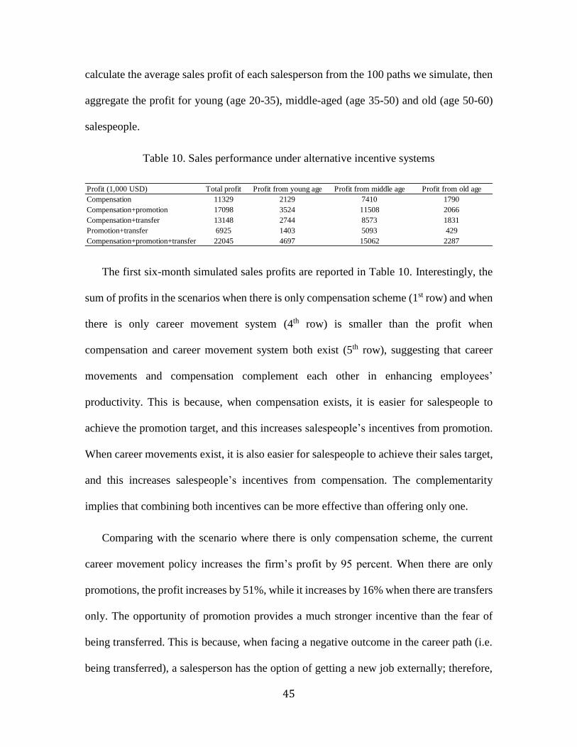
calculate the average sales profit of each salesperson from the 100 paths we simulate, then

aggregate the profit for young (age 20-35), middle-aged (age 35-50) and old (age 50-60)

salespeople.

Table 10. Sales performance under alternative incentive systems

The first six-month simulated sales profits are reported in Table 10. Interestingly, the

sum of profits in the scenarios when there is only compensation scheme (1st row) and when

there is only career movement system (4th row) is smaller than the profit when

compensation and career movement system both exist (5th row), suggesting that career

movements and compensation complement each other in enhancing employees’

productivity. This is because, when compensation exists, it is easier for salespeople to

achieve the promotion target, and this increases salespeople’s incentives from promotion.

When career movements exist, it is also easier for salespeople to achieve their sales target,

and this increases salespeople’s incentives from compensation. The complementarity

implies that combining both incentives can be more effective than offering only one.

Comparing with the scenario where there is only compensation scheme, the current

career movement policy increases the firm’s profit by 95 percent. When there are only

promotions, the profit increases by 51%, while it increases by 16% when there are transfers

only. The opportunity of promotion provides a much stronger incentive than the fear of

being transferred. This is because, when facing a negative outcome in the career path (i.e.

being transferred), a salesperson has the option of getting a new job externally; therefore,

Profit (1,000 USD) Total profit Profit from young age Profit from middle age Profit from old age

Compensation 11329 2129 7410 1790

Compensation+promotion 17098 3524 11508 2066

Compensation+transfer 13148 2744 8573 1831

Promotion+transfer 6925 1403 5093 429

Compensation+promotion+transfer 22045 4697 15062 2287

46

the incentive from the demotion is less powerful than the incentive from the promotion.

Furthermore, the profit increase, when promotions and transfers both exist, is larger than

the sum of the profit increases in the scenarios of promotions or transfers alone, indicating

that both types of career movements can complement each other to incentivize employees’

effort. This is because when promotion opportunities exist, transfer becomes a harsher

punishment to salespeople due to the loss of promotion opportunities after transfer. These

results suggest that not only promotions but also demotions should be used as incentives.

As expected, career movements have a large influence on the work performance for

young and middle-aged salespeople. For salespeople who are close to the age of retirement,

however, promotions and transfers only have a marginal effect. For those salespeople, the

compensation scheme is a far more effective instrument to incentivize their work effort.

These findings imply that it is important for the firm to offer both short-term incentives

(from the compensation) and long-term incentives (from career movements) as a package

in the contract.

5.3. Decomposing the success of the reform

We have shown that career movements are an important component in the incentive system.

We further investigate in this section the contribution of the various incentives to the

success of the reform, as we documented in the data section through the reduced-form

analysis. As shown in the data section, the reform has revamped the structure of the

compensation scheme and career movement policies, including how the base wage is

adjusted and how to promote or transfer salespeople. Until now, it is unclear what are the

effects of these changes on the firm’s profit.

47

The reform on career movements has changed the mix of workers in the sales job

through a new system for promotions and transfers. This will have an impact on the overall

performance. To focus on the effects from incentives and minimize the impact from the

change in the mix of salespeople, we use a series of counterfactuals to decompose the

effects from the reform. We assume that, starting from the first month after the reform,

actual promotions and transfers follow the new policy. In scenario (1), we assume that the

compensation scheme and the evolution of the base wage remain unchanged as before the

reform, and salespeople assume that promotions and transfers are determined in the old

way. Like the simulation procedure described in the previous section, we simulate for each

salesperson 100 paths of sales profit, wage growths, and career movements, then sum up

their sales profits, averaged over the 100 simulations, for the young (age 20-35), middle-

aged (age 35-50) and old (age 50-60) salespeople. The total profit is denoted as 𝑦(1). In

scenario (2), we assume that the compensation scheme has changed, but the evolution of

the base wage remains unchanged and salespeople assume that promotions and transfers

are determined in the old way. The total profit simulated in this scenario is denoted as 𝑦(2).

The difference with the former scenario, i.e., 𝑦(2) − 𝑦(1), represents the effect from the

change in the compensation scheme. In scenario (3), we change both the compensation

scheme and how the base wage is adjusted, but assume that salespeople still expect

promotions and transfers are as before. As the base wage is adjusted differently, the

expectation for promotions and transfer will also change. To make sure that the incentive

from promotions and transfers remains the same as before the reform, we assume that

salespeople use a different base wage that evolves following the old way before the reform,

to form the expectation for their promotions and transfers. The total profit simulated in this

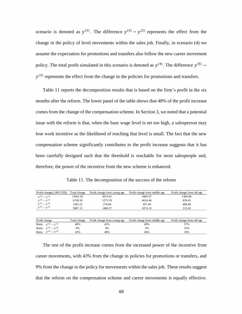
48

scenario is denoted as 𝑦(3) . The difference 𝑦(3) − 𝑦(2) represents the effect from the

change in the policy of level movements within the sales job. Finally, in scenario (4) we

assume the expectation for promotions and transfers also follow the new career movement

policy. The total profit simulated in this scenario is denoted as 𝑦(4). The difference 𝑦(4) −

𝑦(3) represents the effect from the change in the policies for promotions and transfers.

Table 11 reports the decomposition results that is based on the firm’s profit in the six

months after the reform. The lower panel of the table shows that 48% of the profit increase

comes from the change of the compensation scheme. In Section 3, we noted that a potential

issue with the reform is that, when the base wage level is set too high, a salesperson may

lose work incentive as the likelihood of reaching that level is small. The fact that the new

compensation scheme significantly contributes to the profit increase suggests that it has

been carefully designed such that the threshold is reachable for most salespeople and,

therefore, the power of the incentive from the new scheme is enhanced.

Table 11. The decomposition of the success of the reform

The rest of the profit increase comes from the increased power of the incentive from

career movements, with 43% from the change in policies for promotions or transfers, and

9% from the change in the policy for movements within the sales job. These results suggest

that the reform on the compensation scheme and career movements is equally effective.

Profit change(1,000 USD) Total change Profit change from young age Profit change from middle age Profit change from old age

13941.83 3015.01 9465.97 1460.86

6749.50 1275.59 4634.46 839.45

1205.22 278.84 457.40 468.98

5987.12 1460.57 4374.12 152.43

𝑦(4) − 𝑦(1)

𝑦(2) − 𝑦(1)

𝑦(3) − 𝑦(2)

𝑦(4) − 𝑦(3)

Profit change Total change Profit change from young age Profit change from middle age Profit change from old age

Ratio: 48% 42% 49% 57%

Ratio: 9% 9% 5% 32%

Ratio: 43% 48% 46% 10%

𝑦(2) − 𝑦(1)

𝑦(3) − 𝑦(2)

𝑦(4) − 𝑦(3)

49

However, the upper panel of Table 11 shows that the simulated profit increase for old

salespeople is much smaller, consistent with the finding from the reduced-form analysis in

Table 8. The likelihood of promotions and transfers is low for old salespeople; therefore,

only 10% of the profit increase comes from the reform on promotions and transfers. The

change in the compensation scheme is the key driver for the success of the reform for this

age group.

5.4. Alternative career movement policies

With the estimates of the utility primitives, we are able to search for alternative career

movement policies that can improve the firm’s profit. In this section, we use policy

experiment to study (1) how to change the way that promotions and transfers are linked to

the work performance of a salesperson. (2) how to change the spread of the post- and pre-

promotion wages. As these policies change, salespeople’s effort will change and thus

influence the number of promotions and transfers created. Since we do not have data on

the costs and benefits for the firm that are associated with the managerial and other non-

sales jobs, we are unable to evaluate how the new promotions and transfers will impact the

firm’s total profit. To solve this problem, we adjust the thresholds up and ul in the career

movement functions (see the discussion after equation (2)) in all of the alternative policies

to make sure the predicted numbers of promotions and transfers are similar to that under

the existing policy. This way the firm does not need to bear the new cost (or benefit) from

creating new managerial and other non-sales job positions.

In the first policy experiment, we focus on how work performance is evaluated. Based

on our understanding, each salesperson is evaluated twice a year based on various criteria

including the sales profit contributed, his level as a salesperson, demographics, and other

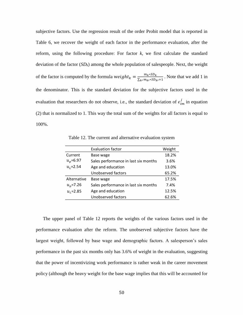
50

subjective factors. Use the regression result of the order Probit model that is reported in

Table 6, we recover the weight of each factor in the performance evaluation, after the

reform, using the following procedure: For factor k, we first calculate the standard

deviation of the factor (SDk) among the whole population of salespeople. Next, the weight

of the factor is computed by the formula w𝑒𝑖𝑔ℎ𝑡𝑘 =𝑚𝑘∗𝑆𝐷𝑘

∑ 𝑚𝑘′∗𝑆𝐷𝑘′𝑘′ +1 . Note that we add 1 in

the denominator. This is the standard deviation for the subjective factors used in the

evaluation that researchers do not observe, i.e., the standard deviation of 𝜖𝑖𝑚𝑗

in equation

(2) that is normalized to 1. This way the total sum of the weights for all factors is equal to

100%.

Table 12. The current and alternative evaluation system

The upper panel of Table 12 reports the weights of the various factors used in the

performance evaluation after the reform. The unobserved subjective factors have the

largest weight, followed by base wage and demographic factors. A salesperson’s sales

performance in the past six months only has 3.6% of weight in the evaluation, suggesting

that the power of incentivizing work performance is rather weak in the career movement

policy (although the heavy weight for the base wage implies that this will be accounted for

Evaluation factor Weight

Current Base wage 18.2%

Sales performance in last six months 3.6%

Age and education 13.0%

Unobserved factors 65.2%

Alternative Base wage 17.5%

Sales performance in last six months 7.4%

Age and education 12.5%

Unobserved factors 62.6%

𝑢𝑝=6.97

𝑢𝐿=2.54

𝑢𝑝=7.26

𝑢𝐿=2.85

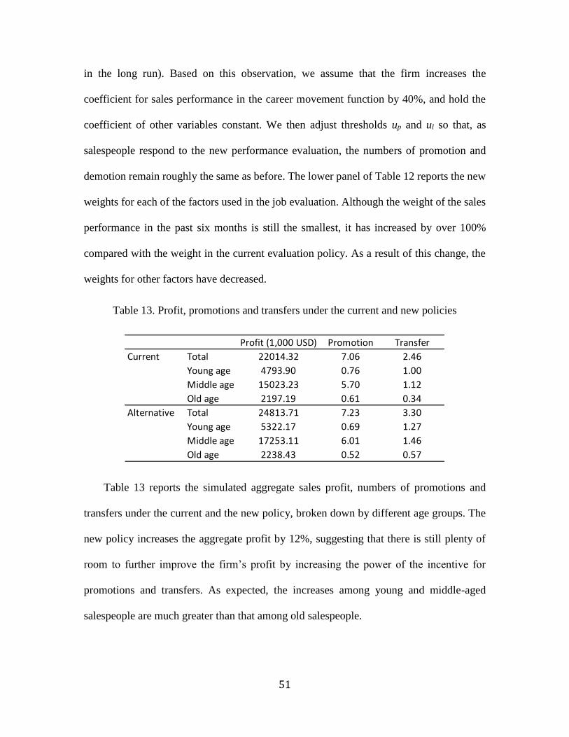
51

in the long run). Based on this observation, we assume that the firm increases the

coefficient for sales performance in the career movement function by 40%, and hold the

coefficient of other variables constant. We then adjust thresholds up and ul so that, as

salespeople respond to the new performance evaluation, the numbers of promotion and

demotion remain roughly the same as before. The lower panel of Table 12 reports the new

weights for each of the factors used in the job evaluation. Although the weight of the sales

performance in the past six months is still the smallest, it has increased by over 100%

compared with the weight in the current evaluation policy. As a result of this change, the

weights for other factors have decreased.

Table 13. Profit, promotions and transfers under the current and new policies

Table 13 reports the simulated aggregate sales profit, numbers of promotions and

transfers under the current and the new policy, broken down by different age groups. The

new policy increases the aggregate profit by 12%, suggesting that there is still plenty of

room to further improve the firm’s profit by increasing the power of the incentive for

promotions and transfers. As expected, the increases among young and middle-aged

salespeople are much greater than that among old salespeople.

Profit (1,000 USD) Promotion Transfer

Current Total 22014.32 7.06 2.46

Young age 4793.90 0.76 1.00

Middle age 15023.23 5.70 1.12

Old age 2197.19 0.61 0.34

Alternative Total 24813.71 7.23 3.30

Young age 5322.17 0.69 1.27

Middle age 17253.11 6.01 1.46

Old age 2238.43 0.52 0.57

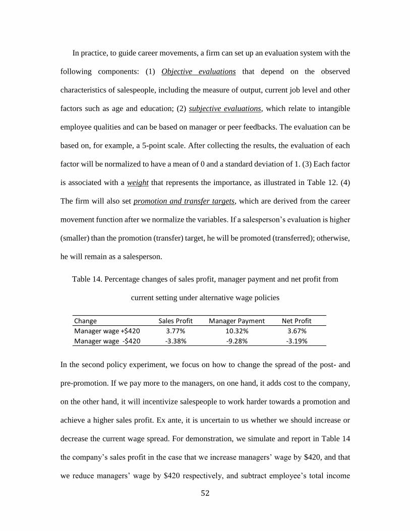
52

In practice, to guide career movements, a firm can set up an evaluation system with the

following components: (1) Objective evaluations that depend on the observed

characteristics of salespeople, including the measure of output, current job level and other

factors such as age and education; (2) subjective evaluations, which relate to intangible

employee qualities and can be based on manager or peer feedbacks. The evaluation can be

based on, for example, a 5-point scale. After collecting the results, the evaluation of each

factor will be normalized to have a mean of 0 and a standard deviation of 1. (3) Each factor

is associated with a weight that represents the importance, as illustrated in Table 12. (4)

The firm will also set promotion and transfer targets, which are derived from the career

movement function after we normalize the variables. If a salesperson’s evaluation is higher

(smaller) than the promotion (transfer) target, he will be promoted (transferred); otherwise,

he will remain as a salesperson.

Table 14. Percentage changes of sales profit, manager payment and net profit from

current setting under alternative wage policies

In the second policy experiment, we focus on how to change the spread of the post- and

pre-promotion. If we pay more to the managers, on one hand, it adds cost to the company,

on the other hand, it will incentivize salespeople to work harder towards a promotion and

achieve a higher sales profit. Ex ante, it is uncertain to us whether we should increase or

decrease the current wage spread. For demonstration, we simulate and report in Table 14

the company’s sales profit in the case that we increase managers’ wage by $420, and that

we reduce managers’ wage by $420 respectively, and subtract employee’s total income

Change Sales Profit Manager Payment Net Profit

Manager wage +$420 3.77% 10.32% 3.67%

Manager wage -$420 -3.38% -9.28% -3.19%

53

from total sales profit to get the net profit. $420 is the current difference between managers’

average income and salespeople’s average income, and we still want to make sure that

managers on average earn more than salespeople when we reduce managers’ wages.

Similar to the previous policy change, for these two alternative wage policies, we also

adjust the promotion and transfer targets to make sure that in equilibrium, the number of

promotions and that of transfers remain similar to that of the current setting. We find that

when we increase managers’ wage, total sales profit will increase by almost 4%. Even

though the company has to pay 10% to managers, the company’s net profit will still be

higher. So the company can expect a higher net profit if it pays more to managers; in other

words, increase the current wage spread.

6 Conclusion

In this paper, we develop and estimate a dynamic structural model and empirically study

the effectiveness of compensation schemes and career movements on the worker

productivity in a Japanese auto sales firm. The hierarchical job structure of firms, together

with the payment structure, provides incentives for better work performance when

employees are forward-looking. Our results show that, relative to the sales job, managerial

jobs bring an employee higher pecuniary and non-pecuniary payoffs, while other non-sales

jobs are worse off in both dimensions. Career concerns are important when salespeople

make the work effort decision, suggesting that long-term incentives can significantly

complement short-term incentives to enhance employees’ productivity. The opportunity of

promotion provides a much stronger incentive to salespeople than the fear of being

transferred. We also find that about half of the profit increase from the firm’s reform comes

from the increased power of the incentive from the compensation scheme, and the rest from

54

the change in the career movement policies. Finally, we illustrate how the firm can

implement an alternative policy for career movements that places more weight on the work

performance to further incentivize the work effort from young and middle-aged salespeople,

and how the company can achieve a higher net profit by increasing the current wage spread

between the post- and pre-promotion job.

This study has several limitations. First, we focus on how compensation and career

movements incentivize the work performance and abstract away from how these policies

create self-selection among employees through accepting contract offers and quitting jobs.

Conceptually, an incentive system weighted more on job performance will attract workers

with higher ability and force those with lower ability to leave. To study such effects we

have to model the intrinsic ability of each worker and their job search decisions. This is out

of the scope of the current study. Furthermore, due to data constraints we are unable to

study the factors that incentivize the performance of employees at the managerial and other

non-sales jobs. Finally, this study is not a direct test of the tournament theory, as we do not

have the required data variation. For example, we do not observe significant changes in the

difference between the pre- and post-promotion wages. These are important venues for

future research.

55

References

Audas, R., Barmby, T., & Treble, J. (2004). Luck, effort, and reward in an organizational

hierarchy. Journal of Labor Economics, 22(2), 379-395.

Baker, G., Gibbs, M., & Holmstrom, B. (1994). The internal economics of the firm:

evidence from personnel data. The Quarterly Journal of Economics, 881-919.

Baker, G., Gibbs, M., & Holmstrom, B. (1994). The wage policy of a firm. The Quarterly

Journal of Economics, 921-955.

Bandiera, O., Barankay, I., & Rasul, I. (2007). Incentives for Managers and Inequality

among Workers: Evidence from a Firm-Level Experiment. The Quarterly Journal of

Economics, 122(2), 729-773.

Basu, A. K., Lal, R., Srinivasan, V., & Staelin, R. (1985). Salesforce compensation plans:

An agency theoretic perspective. Marketing science,4(4), 267-291.

Becker, G. S. (2009). Human capital: A theoretical and empirical analysis, with special

reference to education. University of Chicago press.

Chan, T. Y., Li, J., & Pierce, L. (2014). Compensation and peer effects in competing sales

teams. Management Science, 60(8), 1965-1984.

Chung, D. J., Steenburgh, T., & Sudhir, K. (2014). Do bonuses enhance sales productivity?

A dynamic structural analysis of bonus-based compensation plans. Marketing

Science, 33(2), 165-187.

Coughlan, A. T., & Narasimhan, C. (1992). An empirical analysis of sales-force

compensation plans. Journal of Business, 93-121.

56

Coughlan, A. T., & Sen, S. K. (1989). Salesforce compensation: Theory and managerial

implications. Marketing Science, 8(4), 324-342.

Doeringer, P. B., & Piore, M. J. (1985). Internal labor markets and manpower analysis.

ME Sharpe.

De Varo, J. (2006). Internal promotion competitions in firms. RAND Journal of

Economics, 521-542.

Gibbons, R., & Murphy, K. J. (1991). Optimal incentive contracts in the presence of career

concerns: Theory and evidence (No. w3792). National Bureau of Economic Research.

Gayle, G. L., Golan, L., & Miller, R. A. (2015). Promotion, turnover, and compensation in

the executive labor market. Econometrica, 83(6), 2293-2369.

Greenwald, B. C. (1986). Adverse selection in the labour market. The Review of Economic

Studies, 53(3), 325-347.

Hölmstrom, B. (1979). Moral hazard and observability. The Bell journal of economics, 74-

91.

Joseph, K., & Kalwani, M. U. (1998). The role of bonus pay in salesforce compensation

plans. Industrial Marketing Management, 27(2), 147-159.

Kandel, E., & Lazear, E. P. (1992). Peer pressure and partnerships. Journal of political

Economy, 801-817.

Lal, R., Outland, D., & Staelin, R. (1994). Salesforce compensation plans: an individual-

level analysis. Marketing Letters, 5(2), 117-130.

57

Lal, R., & Srinivasan, V. (1993). Compensation plans for single-and multi-product

salesforces: An application of the Holmstrom-Milgrom model. Management

Science, 39(7), 777-793.

Lazear, E. P. (1986). Salaries and piece rates. Journal of business, 405-431.

Lazear, E. P. (2000). The power of incentives. The American Economic Review, 90(2),

410-414.

Lazear, E. P., & Rosen, S. (1981). Rank-order tournaments as optimum labor contracts.

Journal of Political Economy, 841–864.

Misra, S., Coughlan, A. T., & Narasimhan, C. (2005). Salesforce compensation: An

analytical and empirical examination of the agency theoretic approach. Quantitative

Marketing and Economics, 3(1), 5-39.

Misra, S., & Nair, H. S. (2011). A structural model of sales-force compensation dynamics:

Estimation and field implementation. Quantitative Marketing and Economics, 9(3), 211-

257.

Paarsch, H. J., & Shearer, B. S. (1999). The response of worker effort to piece rates:

evidence from the British Columbia tree-planting industry.Journal of Human Resources,

643-667.

Paarsch, H. J., & Shearer, B. (2000). Piece rates, fixed wages, and incentive effects:

Statistical evidence from payroll records. International Economic Review, 41(1), 59-92.

Rao, R. C. (1990). Compensating heterogeneous salesforces: Some explicit

solutions. Marketing Science, 9(4), 319-341.

58

Shearer, B. (2004). Piece rates, fixed wages and incentives: Evidence from a field

experiment. The Review of Economic Studies, 71(2), 513-534.

Waldman, M. (1984). Job assignments, signalling, and efficiency. The RAND Journal of

Economics, 15(2), 255-267.

Zoltners, A. A., Sinha, P., & Lorimer, S. E. (2008). Sales force effectiveness: A framework

for researchers and practitioners. Journal of Personal Selling & Sales Management, 28(2),

115-131.

Documents

Incentives from Compensation and Career Movements on Work