INCIDENT DATA ANALYSIS USING DATA MINING TECHNIQUES

A Thesis

by

LISA M. VELTMAN

Submitted to the Office of Graduate Studies of Texas A&M University

in partial fulfillment of the requirements for the degree of

MASTER OF SCIENCE

August 2008

Major Subject: Safety Engineering

INCIDENT DATA ANALYSIS USING DATA MINING TECHNIQUES

A Thesis

by

LISA M. VELTMAN

Submitted to the Office of Graduate Studies of Texas A&M University

in partial fulfillment of the requirements for the degree of

MASTER OF SCIENCE

Approved by:

Chair of Committee, M. Sam Mannan Committee Members, Marietta J. Tretter Mahmoud El-Halwagi Head of Department, Michael Pishko

August 2008

Major Subject: Safety Engineering

iii

ABSTRACT

Incident Data Analysis Using Data Mining Techniques. (August 2008)

Lisa M. Veltman, B.S., Texas A&M University

Chair of Advisory Committee: Dr. M. Sam Mannan

There are several databases collecting information on various types of incidents, and

most analyses performed on these databases usually do not expand past basic trend

analysis or counting occurrences. This research uses the more robust methods of data

mining and text mining to analyze the Hazardous Substances Emergency Events

Surveillance (HSEES) system data by identifying relationships among variables,

predicting the occurrence of injuries, and assessing the value added by the text data. The

benefits of performing a thorough analysis of past incidents include better understanding

of safety performance, better understanding of how to focus efforts to reduce incidents,

and a better understanding of how people are affected by these incidents.

The results of this research showed that visually exploring the data via bar graphs did not

yield any noticeable patterns. Clustering the data identified groupings of categories

across the variable inputs such as manufacturing events resulting from intentional acts

like system startup and shutdown, performing maintenance, and improper dumping.

Text mining the data allowed for clustering the events and further description of the data,

however, these events were not noticeably distinct and drawing conclusions based on

these clusters was limited. Inclusion of the text comments to the overall analysis of

HSEES data greatly improved the predictive power of the models. Interpretation of the

textual data’s contribution was limited, however, the qualitative conclusions drawn were

similar to the model without textual data input. Although HSEES data is collected to

describe the effects hazardous substance releases/threatened releases have on people, a

fairly good predictive model was still obtained from the few variables identified as cause

related.

iv

DEDICATION

To Mom and Dad

v

ACKNOWLEDGEMENTS

I would like to thank my advisor Dr. M. Sam Mannan for his guidance and support in

my research and academic developments as well as allowing me the opportunity to be a

part of the Mary Kay O’Connor Process Safety Center. Thanks to my committee

member Dr. Marietta J. Tretter for all of her help and advice about both my research and

challenges life may bring. Thanks to my other committee member Dr. Mahmoud El-

Halwagi for his support in my research endeavors. Also, many thanks to Mr. T. Michael

O’Connor for the thought provoking discussions, advice on my research, and for

allowing me the privilege to participate in projects the Center is involved in.

I would also like to thank Donna Startz, Mary Cass, and Valerie Green for all of the

assistance they have provided me over the course of my graduate studies at Texas A&M

University. Thanks to Dr. William J. Rogers for the long discussions about my research,

safety in general, and all of the other interesting adjacent topics that came up.

I would like to thank my friends and fellow students in the Center for their support,

encouragement, camaraderie, and for making my experience in our research group an

enjoyable one.

Finally, thanks to Mom and Dad for their everlasting love, support, and encouragement.

vi

TABLE OF CONTENTS

Page

ABSTRACT ..................................................................................................................... iii

DEDICATION ..................................................................................................................iv

ACKNOWLEDGEMENTS ...............................................................................................v

LIST OF FIGURES........................................................................................................ viii

LIST OF TABLES ............................................................................................................ix

1. INTRODUCTION.........................................................................................................1

2. BACKGROUND...........................................................................................................3

3. HSEES DATA...............................................................................................................7

4. DATA MINING............................................................................................................9

4.1 Describing the Data..........................................................................................9 4.1.1 Variables............................................................................................9 4.1.2 Visualization and Summaries..........................................................10 4.1.3 Clustering ........................................................................................10 4.1.4 Text Mining.....................................................................................10

4.2 Building Predictive Models............................................................................12 4.2.1 Decision Trees.................................................................................12 4.2.2 Logistic Regression .........................................................................13

4.3 Measuring Model Performance ......................................................................13 4.3.1 Lift and Gain ...................................................................................13 4.3.2 Maximum Likelihood Estimates .....................................................17

5. METHODS..................................................................................................................18

5.1 Define Data Mining Goal ...............................................................................18 5.2 Data Cleaning and Preparation.......................................................................19 5.3 Data Analysis .................................................................................................21

vii

6. RESULTS....................................................................................................................22

6.1 Sample............................................................................................................22 6.2 Explore and Modify .......................................................................................22

6.2.1 MultiPlot..........................................................................................24 6.2.2 Clustering ........................................................................................29 6.2.3 Text Mining.....................................................................................32

6.3 Model .............................................................................................................37 6.3.1 Decision Tree without Text Input ...................................................37 6.3.2 Decision Tree with Text Input ........................................................40 6.3.3 Logistic Regression Node without Text Input ................................44 6.3.4 Logistic Regression Node with Text Input .....................................50

6.4 Assess .............................................................................................................53

7. CONCLUSIONS AND RECOMMENDATIONS......................................................56

7.1 Conclusions ....................................................................................................56 7.2 Recommendations ..........................................................................................57

REFERENCES.................................................................................................................58

VITA ................................................................................................................................60

viii

LIST OF FIGURES

Page

Figure 1 Example of Cumulative Gain Chart........................................................15

Figure 2 Example of Lift Chart .............................................................................16

Figure 3 Primary Factor by Injury Occurrence .....................................................26

Figure 4 Secondary Factor by Injury Occurrence .................................................27

Figure 5 Industry Code by Injury Occurrence ......................................................28

Figure 6 Spills by Injury Occurrence ....................................................................29

Figure 7 Air Emissions by Injury Occurrence ......................................................29

Figure 8 Clustered Data.........................................................................................30

Figure 9 Cluster Rings...........................................................................................35

Figure 10 Cumulative Lift Comparison for Train Dataset ......................................54

Figure 11 Cumulative Lift Comparison for Validate Dataset .................................54

Figure 12 Cumulative Lift Comparison for Test Dataset........................................55

ix

LIST OF TABLES

Page

Table 1 Term Frequency Matrix ..........................................................................11

Table 2 Example of Calculated Lift Values .........................................................15

Table 3 Categorical Variables ..............................................................................23

Table 4 Continuous Variables ..............................................................................24

Table 5 Events per Hazardous Substance Subcategory........................................25

Table 6 Clustered Terms per Segment .................................................................33

Table 7 Cluster Descriptions ................................................................................34

Table 8 Classifications for Decision Tree with No Text Input ............................37

Table 9 Variable Importance for Decision Tree with No Text Input...................38

Table 10 Classifications for Decision Tree with Text Input ..................................41

Table 11 Variable Importance for Decision Tree with Text Input.........................42

Table 12 Cluster Weights for SVD_1 and SVD_4 ................................................43

Table 13 Classifications for Logistic Regression with No Text Input ...................45

Table 14 Maximum Likelihood Estimates for Logistic Regression without Text .46

Table 15 Reduced Variable List for Logistic Regression with No Text Input ......48

Table 16 Classifications for Logistic Regression with Text Input.........................50

Table 17 Maximum Likelihood Estimates for Logistic Regression with Text ......51

Table 18 Reduced Variable List for Logistic Regression with Text Input ............52

1

1. INTRODUCTION

There is a need to understand how industry as a whole is performing from a safety

standpoint. To date, no one can really answer this question with certainty. People do a

decent job collecting data on incidents, but few take the analyses of the data past basic

trending. Having the capability to collect enormous amounts of data is a feat in and of

itself; however, it begs the question, “So what?” With the amount of resources spent to

collect data, it seems logical to look at the data under extreme scrutiny to obtain as much

knowledge about the data as possible. Data in a database is just that, data. By analyzing

and understanding what is in the database yields knowledge. Passing this knowledge on

to others can improve the understanding of what went wrong with incidents from the

past thereby greatly enabling the prevention of future incidents.

Trending analyses do provide useful comparisons in the data, however, going beyond

comparisons by using data mining techniques can enable one to build predictive models,

unveil relationships within the data that are not necessarily intuitive, and perhaps answer

the question, “How is industry’s safety performance doing?” Marketers have

successfully harnessed the power of data mining to build predictive models to increase

profit by, for example, determining customer buying habits based on advertisement

campaigns. The advantage of using data mining is its ability to analyze an enormous set

of data [1]. Using the data mining as an analysis tool applied to incident databases can

make a huge, positive impact on industry and the public at large.

The benefits of performing a thorough analysis of incident databases include better

understanding of safety performance, better understanding of how to focus efforts to

____________ This thesis follows the style of Journal of Hazardous Materials.

2

reduce incidents, and a better understanding of how people are affected by these

incidents. The data chosen for this research comes from the Hazardous Substances

Emergency Events Surveillance (HSEES) system for the years 2002 to 2004. This

system collects data on incidents where there was a release or threatened release of a

hazardous substance that resulted in some public health action [2]. It is unique in that it

collects data for the purpose of analyzing the effects these incidents have on the health of

the public as opposed to other databases that focus on environmental impact.

The objective of this research is to use data mining and text mining to analyze the

HSEES system data by identifying relationships among the variables, predicting

variable(s) of interest, and assessing the value added by the text data. Furthermore, the

results of this research will define what can be done with this type of data in terms of

analyses and what types of questions more thorough analyses may answer.

3

2. BACKGROUND

Analyses of the information in databases help connect the dots between what went

wrong and what people can do to prevent it—the relationship between the cause of an

incident and its consequences. Trevor Kletz time and time again reminds us that an

essential part of not repeating mistakes from history is to make sure that lessons are

learned, and to make sure these lessons are shared as new generations join in. Several

people have put their mark on assessing what knowledge is available from incident

databases and some of these are discussed in the following.

Eboni Trevette McCray compared several incident databases in an effort to formulate

improvements for these databases as well as determine national safety goals to be

implemented given these improvements. It was argued that comparing and trending data

from the databases is impossible due to the overall discrepancy in data collection

agendas, methods, and definitions from year to year. As a result, it was proposed to

create a single database with a thorough amount of information on incident details

including the causes and effects of the incidents. This proposed database will originate

from the existing Emergency Response Notification System (ERNS) database and is

expanded upon with questions from an Accidental Release Information Program (ARIP)

survey [3]. Although it is agreed that there are errors and discrepancies in data

collection, it is disagreed that ascertaining any useful analysis from these databases is

impossible. It is implicit through modeling these data that there is some level of

variability and uncertainty, yet the overall trend and relationships will be foretelling

enough to draw conclusions and make recommendations for safer practices regarding

chemicals. In the case of my research, the data used from 2002 to 2004 have common

definitions and the inherent nature of HSEES being an active system means the data are

more reliable.

4

Others have made strides to analyze databases such as Fahad Al-Qurashi’s work where

the combined effects of accidental, failure rate, and reactive chemical databases were

considered. Specifically, the Environmental Protection Agency’s (EPA) Risk

Management Program (RMP) database was used to decipher the most significant

chemicals released and ultimately it was concluded that there is a need for more data

with regard to failure rates and reactive chemicals. It was stressed that with the

appropriate understanding of equipment reliability and the inherent hazards of chemicals

used, the number of incidents can be reduced [4]. Although the focus of this research is

to link different data sources together to find new learnings, it still identified the most

frequently occurring offenders and basic trends with the analysis, but did not incorporate

predictive modeling.

Looking at the benefits of using data mining, one can consider Sumit Anand’s work

where data mining techniques were applied to the National Response Center’s database

to uncover interesting patterns in data pertaining to fixed facilities in Harris County,

Texas from 1990-2002. Example techniques applied to these data are decision trees

where consequences of an incident are compared to the type of equipment failure and

incident cause, and association analysis used to compare the type of equipment failure

and the chemical involved. Using the data mining results, Anand updated equipment

failure probabilities and built a decision support system [5]. Finding associative

behaviors between variables, like type of injury and chemical released, might be a viable

option for the HSEES dataset. It could show how likely the presence of some chemical

X will result in some injury y. An alternative option is clustering events.

Terry L. Bunn et al analyzed tractor fatality data for the state of Kentucky focusing on

the added benefits of analyzing the text given by way of incident investigation reports.

They showed that analyzing text entries in addition to coded data provides far more

information then looking at coded data alone [6]. The advantage with the tractor fatality

dataset is that the text entries are detailed incident investigation reports, not short

5

comments on the nature of the event like what is contained in the HSEES dataset.

Relationships in the tractor data were extracted about pre-event, event, and post-event

conditions, namely the initiating event, the actual injury or outcome, and the response to

the event. The consequence of “Dead at the scene” events were linked with the causes

“operation of a tractor with a bucket, muddy terrain, and being thrown from the tractor”

[6]. Causes of dying from being “crushed” were identified as “the lack of tractor

maintenance, the lack of brakes, or a clutch as well as the lack of a seat belt on the

tractor, the lack of an attached [rollover protective structure], the lack of tractor

counterweights for tractor balance, overturning the tractor, and operating the tractor on

an embankment or a slope” [6]. Using logistic regression analysis, it was found that an

individual is 8.8 times more likely to die of being crushed where the tractor is overturned

or rolled over, and that a driver is more likely to be crushed when operating on a slope

than on level ground [6]. This example goes to show the benefits for including the

analysis of text data in finding patterns and building models. A similar approach is used

to combine the HSEES text comments with the other structured data to build a predictive

model.

Already the HSEES data is benefitting the public at large. The Agency for Toxic

Substances and Disease Registry (ATSDR) produces annual reports from the HSEES

data. These reports include things such as the number of victims and types of injuries,

the types of substances released, the number of evacuations, and information on the most

commonly reported category of substances [7]. In addition to the ATSDR report,

participating states are required to analyze the data and use their findings for outreach

programs [2]. Doing so ensures that the data collected is used to benefit the public.

States like New York have done an excellent job with their analysis to accomplish things

such as removal of mercury from schools and identifying sources of carbon monoxide

poisoning in buildings [8].

6

ASM Obidullah analyzed the HSEES data by considering the relationship between the

causes and consequences of the recorded incidents for Texas manufacturing facilities as

well as proposed a national estimate. In this research, trend, cause, and consequence

analysis were used to conclude and recommend further study and integration of

equipment failure data, the need for more training on safe practices when conducting

maintenance and further study of the environmental impact chemical releases are having

since many of the releases in the HSEES database did not have recorded injuries. Some

of the findings were that equipment failure was a major cause for process interruption,

process upset is the most frequent type of process interruption in the industries analyzed,

and respiratory irritation was the type of injury that frequently occurred among workers

[9]. Obidullah made good progress in the effort to learn from past manufacturing

incidents from the HSEES database, however, more learning can be wrought from this

database by using the predictive power that data mining can provide.

The commonality between all of these works is that society as a whole can learn from

past incidents through data analysis in order to prevent future incidents from occurring.

There is an enormous potential to learn from the information housed in today’s databases

with the wide availability of various approaches. Analyses that are done on data such as

HSEES are just scratching the surface. Ramping up these analyses with analyses that

data mining can help produce will further help meet the overall goal with any type of

analyses—taking data and gaining knowledge from it. In the case of analyses on the

HSEES data, the idea is to gain knowledge and understandings of incidents such that one

can identify what areas need to be focused on to reduce the occurrences of harm to the

public. Adding predictive power to the reports and findings that are currently available

will greatly aid in this effort.

7

3. HSEES DATA

The Hazardous Substances Emergency Events Surveillance (HSEES) data includes

information on events where:

• There was an uncontrolled/illegal release or threatened release of at least one

hazardous substance NOT including petroleum (due to the Petroleum Exclusion

clause of CERCLA) and the release of the hazardous substance(s) requires

removal, clean up, or neutralization, or

• There was a threatened release of a hazardous substance that would have needed

to be removed, cleaned up, or neutralized AND the threatened release resulted in

a public health action.

Although CERCLA has a Petroleum Exclusion, events where petroleum is released

along with other hazardous substances are included in HSEES and petroleum is reported

along with the other substances [2].

HSEES is unique compared to other databases since its focus is on public health whereas

other databases focus on environmental impact. This focus on public health is aligned

with ATSDR’s mission “to serve the public by using the best science, taking responsive

public health actions, and providing trusted health information to prevent harmful

exposures and disease related to toxic substances” [2]. The purpose for collecting the

data is to assess the acute effects hazardous substance emergencies have on the

morbidity and mortality of the first responders, general public, and employees, and

thereby reduce these occurrences [2].

The data for 2002 to 2004 were obtained in an excel spreadsheet format. There are four

different worksheets: event data, chemical data, victim data, and text comments. The

event data includes information on unique record number for each incident, the type of

event (fixed facility or transportation), whether there was an actual release or a

threatened release, location, the type of area, time, date, and day of the week the event

8

occurred, type of industry, and contributing factors to the incident. The latter is not to be

confused with root causes as a more thorough investigation is required to find this type

of information. These data are formatted such that each row represents a single event.

The chemical data contain information such as the unique record number, type of

chemical released, the chemical category, and the quantity of the chemical released.

Each row in the chemical dataset represents a single chemical involved in the incident.

Incidents with several chemicals involved will have several rows of data in the chemical

file.

The victim data contain the unique record number, specific information on the types of

injuries incurred, the type of personal protective equipment (PPE) used if at all,

decontaminations, whether or not an evacuation or shelter-in-place was ordered, age and

gender of the victim, victims distance from the event, and type of victim (first responder,

general public, employee, or student). Each row of data in this dataset represents a

single victim. Consequently, the victim data will have multiple rows for a single

incident if there are multiple victims.

The text worksheet contains the record number and the text comment inputted for the

incident. The formatting of this file is inconsistent. Text comments for a single incident

were in most cases split into different cells on different rows and columns within the

spreadsheet. Heavy cleaning was necessary to get the comments rejoined into a single

cell for each subsequent event. Once cleaned, these data will have a single row per

incident.

9

4. DATA MINING

The capabilities of generating and collecting data has rapidly grown in the last couple of

decades and as such there is a need for technology that can assist a user by transforming

large amounts of data into useful information [10]. Cue data mining. Data mining can

be defined as “the process of discovering interesting knowledge from large amounts of

data stored either in databases, data warehouses, and other information repositories”

[10]. The process can be described in three steps—describe the data, build a predictive

model, and verify the model. Data are described by its statistical attributes such as

means and standard deviations, by visually reviewing charts and graphs, and looking for

relationships among variables. Predictive models are built based on patterns found in

known results. The model must be tested with a separate data sample that was not used

to build the model and contains known results. Finally, the model should be verified

with new data without known results [11].

4.1 Describing the Data

Visualization, summaries, and cluster analysis are used to describe the structured HSEES

data. Text mining is used to describe the unstructured data in HSEES. These methods

are described in the following sections.

4.1.1 Variables

Structured data consist of three main types of variables—nominal, ordinal, and

continuous. Nominal variables are unordered categorical variables, ordinal variables are

ordered categorical variables, and continuous variables are numeric [11]. Examples of

nominal variables are names or type of event (fixed facility versus transportation event).

Examples of ordinal variables include class ranks and letter grades. Continuous

10

variables are attributes such as age or temperature. Data such as text comments are

considered unstructured data.

4.1.2 Visualization and Summaries

Plots and graphs are used to visually compare different groups of variables. Visualizing

the data in this way is helpful particularly because patterns and relationships are easier to

perceive graphically then they are when looking at text or numerical values. Visualizing

the data and looking at the statistical summaries is extremely beneficial with promoting

understanding of the data, because it helps the modeler easily recognize patterns or

relationships that might otherwise go unnoticed [11].

4.1.3 Clustering

The intention of clustering a database is to divide data into groups that are distinct from

one another, but whose elements are similar. Furthermore, the idea is to segment the

data into groups that are not previously defined so that the clusters can be used to

classify new data. This might require excluding variables that are not meaningful or

otherwise insignificant until reasonable clusters are formed [11]. SAS displays attributes

in each cluster using bar graphs that the modeler can use to ascertain the distinctness of

the clusters.

4.1.4 Text Mining

Text mining is used to find patterns in unstructured data. Common problems with

analyzing textual data are misspellings, synonymy, and polysemy (same word can have

different meanings in different contexts) [10]. The text mining node in SAS creates a

term frequency matrix and displays a term table that shows the total number of times

each term appears and the number of documents the term appears in. Synonym lists,

11

stop lists, and start lists can be created and implemented to guide what terms the text

mining node groups together (synonym list), what terms to omit because they are

deemed irrelevant (stop list), and what terms to keep (start list). Furthermore, the text

mining node may be set up to automatically cluster, allowing for closer inspection of the

documents that contain similar sets of words.

One method of structuring text data to incorporate into models is to use latent semantic

indexing (LSI). The LSI method uses the technique of singular value decomposition

(SVD) to reduce the size of the term frequency matrix [10]. As depicted in Table 1

below, the n x m term frequency matrix shows the frequency (ai,j) of terms (ti) per

document (dj).

Table 1 Term Frequency Matrix

Frequencies d1 d2 d3 d4 d5 … dm

t1 a 1,1 a 1,2 a 1,3 a 1,4 a 1,5 … a 1,m

t2 a 2,1 a 2,2 a 2,3 a 2,4 a 2,5 … a 2,m

t3 a 3,1 a 3,2 a 3,3 a 3,4 a 3,5 … a 3,m

t4 a 4,1 a 4,2 a 4,3 a 4,4 a 4,5 … a 4,m

t5 a 5,1 a 5,2 a 5,3 a 5,4 a 5,5 … a 5,m

… … … … … … … …tn a n,1 a n,2 a n,3 a n,4 a n,5 … a n,m

For example, there are a1,1 occurrences of the term t1 in document d1. The SVD method

takes this n x m matrix and reduces it to a K x K matrix by removing rows and columns

with the least significant information. The latent semantic indexing method can be

generalized to the following steps:

1. Create a term frequency matrix.

2. Compute SVD of the term frequency matrix by splitting the matrix into three

matrices, U, S, and V. U and V are orthogonal matrices (UTU=1 and

VTV=1), and S is the reduced K x K matrix.

12

3. Replace each document d’s vector by a new one that excludes the terms

eliminated during SVD.

4. Store the set of all vectors and index them using advanced multi-dimensional

indexing techniques [10].

SAS Text Miner node performs these functions and the new SVD variables can be used

as input in subsequent nodes that build the predictive models.

4.2 Building Predictive Models

Logistic regression and decision trees are two methods of building predictive models.

4.2.1 Decision Trees

Decision trees can predict categorical or continuous variables. The decision trees

represent a series of rules that lead to some class or value. The top node is the decision

node, which specifies the test to be carried out. Each branch off of the top node leads to

either another decision node or to the leaf node (at the end of a branch). The trees are

grown with an iterative process that splits the data into discrete groups with the “goal to

maximize ‘distance’ between groups at each split” [11].

To control the size of the tree, stopping rules may be implemented such as limiting the

depth the tree may grow to. The tree may also be pruned—the modeler or the built-in

heuristics can prune the tree to the smallest size that still maintains its accuracy [11].

A drawback of using decision trees are that they do not consider the effects splits might

have on future splits. Furthermore, the tree makes splits sequentially resulting in each

split being dependent on its predecessor. Thus, changing a split somewhere in the tree

can greatly impact the resulting splits after it. Although the model builds quickly since it

considers a single predictor variable at a time, this limits the number of splitting rules to

13

test as well as increases the difficulty of detecting relationships among predictor

variables [11].

4.2.2 Logistic Regression

Logistic regression is used to predict binary variables with values yes/no or 1/0.

Because the target variable is not continuous, it cannot be predicted with linear

regression. Instead, logistic regression predicts the logarithm of the odds of the event

occurring as opposed to predicting if the event will occur. The logarithm is referred to

as the log odds or logit transformation and is expressed as the following ratio of

probabilities:

)Pr()Pr(

occurnotdoeseventoccurseventratioodds =

For example, if the odds ratio is 3, then the probability of the event occurring is three

times as much as the probability of the event not occurring. In other words, the odds are

3 to 1 that the event will occur, or there is a 75% chance the event will occur and 25%

chance it will not [11].

4.3 Measuring Model Performance

This section discusses the metrics used to decipher how well a predictive model has

performed.

4.3.1 Lift and Gain

Lift is the ratio of the target response to the average response of the population. It can be

expressed as lift per decile or as the cumulative lift across the population. Gain

14

describes the ratio of the target response to the total number of positive responses.

These are defined in the following equations:

baLift i=

nb

aLiftCumulative

n

ii

*1∑==

A

aGainCumulative

n

ii∑

== 1

where ia = number of predicted positive responses in decile i

TAb = , the total number of positive responses A per total events T

n = is the decile being considered.

Typically lift is illustrated using cumulative gains and lift charts. To demonstrate these

calculations and the resulting charts, consider Table 2, which is populated with fictitious

data. Consider decile 3 in Table 2. The lift is 240/160 = 1.5, the cumulative lift is

1,040/480 = 2.2, and the cumulative gain is 1,040/1,600 = 65%.

15

Table 2 Example of Calculated Lift Values

DecileTotal

Number of Events

Predicted Positive

Responses

Average Positive

Response

Cumulative Gains

Cumulative Lift

Predicted Positive

Responses

Average Positive

ResponseLift

0 0 0 0 0 0 1 2,000 480 160 30% 3.0 480 160 3.0 2 4,000 800 320 50% 2.5 320 160 2.0 3 6,000 1,040 480 65% 2.2 240 160 1.5 4 8,000 1,264 640 79% 2.0 224 160 1.4 5 10,000 1,360 800 85% 1.7 96 160 0.6 6 12,000 1,440 960 90% 1.5 80 160 0.5 7 14,000 1,504 1,120 94% 1.3 64 160 0.4 8 16,000 1,552 1,280 97% 1.2 48 160 0.3 9 18,000 1,584 1,440 99% 1.1 32 160 0.2 10 20,000 1,600 1,600 100% 1.0 16 160 0.1

Cumulative by Decile By Decile

The data in the table for all 10 deciles yield the cumulative gain chart found in Figure 1

and the lift chart in Figure 2.

Cumulative Gains

0%

10%

20%

30%

40%

50%

60%

70%

80%

90%

100%

1 2 3 4 5 6 7 8 9 10

Decile

% T

otal

Eve

nts

Lift Curve Baseline

Figure 1 Example of Cumulative Gain Chart

16

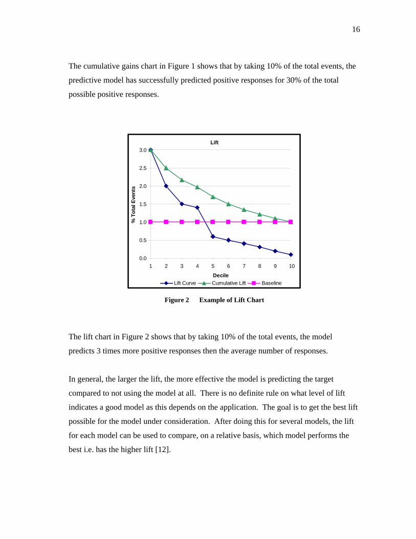
The cumulative gains chart in Figure 1 shows that by taking 10% of the total events, the

predictive model has successfully predicted positive responses for 30% of the total

possible positive responses.

Lift

0.0

0.5

1.0

1.5

2.0

2.5

3.0

1 2 3 4 5 6 7 8 9 10

Decile

% T

otal

Eve

nts

Lift Curve Cumulative Lift Baseline

Figure 2 Example of Lift Chart The lift chart in Figure 2 shows that by taking 10% of the total events, the model

predicts 3 times more positive responses then the average number of responses.

In general, the larger the lift, the more effective the model is predicting the target

compared to not using the model at all. There is no definite rule on what level of lift

indicates a good model as this depends on the application. The goal is to get the best lift

possible for the model under consideration. After doing this for several models, the lift

for each model can be used to compare, on a relative basis, which model performs the

best i.e. has the higher lift [12].

17

4.3.2 Maximum Likelihood Estimates

Maximum likelihood estimates are convenient for determining whether the predictor

variables in the model are statistically significant. These estimates are provided in the

output for the logistic regressions. To check for statistical significance, the modeler can

review the p-values for each predictor variable used in the model. A value less than 0.05

means the variable is statistically significant. The odds ratio is given for each variable,

and this number indicates the relative importance of each variable’s contribution to the

overall response prediction. Ideally, the modeler will want several variables to

contribute importantly to the overall model. The other measurements used to assess the

model’s predictive ability are found in the association of the predicted probabilities and

actual responses statistics, which can show what percent of the predicted probabilities

matched the actual responses [13].

18

5. METHODS

Data mining is a method to find patterns in data and build predictions using these

patterns. The general steps are first to describe the data in terms of its statistical

attributes, visually look at charts and graphs to identify meaningful relationships among

the variables, build predictive models based on the patterns found, test if the model

appropriately predicts variables using known data separate from the data used to build

the model, and finally verify the model with real data [11].

For this project, a similar approach is used and it is summarized in the following steps:

1. Define a data mining goal.

2. Clean the data and prepare it for analysis.

3. Choose samples to analyze.

4. Look for patterns and relationships.

5. Modify dataset as necessary.

6. Apply models to the dataset.

7. Assess how well these models fit the data.

8. Compare the data mining results to previous work.

Steps 2 through 6 can be repeated as necessary to develop a reasonable model and details

of the steps are provided later.

5.1 Define Data Mining Goal

Before beginning the data mining process, a clear, well-defined objective must be

established. The objective for the data and text mining is to build a model that predicts

whether an event will result in injured or killed victims. More specifically, the goal is to

build a model that relates whether victims are injured or killed, a consequence, to event

characteristics that logically can be considered causal information. Three variables that

could be used as targets for such an assessment are the total victims (a number), whether

19

there was an injury (yes/no), and whether there was a fatality (yes/no). Closer inspection

of the data revealed that only 49 events out of 19,165 resulted in at least one fatality

(0.3% of the total events) and 1,592 events out of 19,165 resulted in an injury (8% of the

total events). Because of the small number of fatalities, the occurrence of fatalities was

omitted as a possible target leaving the number of victims and occurrence of an injury.

The decision was made to predict the occurrence of an injury since it is binary and will

result in a simpler model.

5.2 Data Cleaning and Preparation

Data cleaning and preparation is the second step in the data mining process. Relative to

this research, step 1 entails consolidating the data into a single flat file with each row of

data representing a single event. Since the event file is already set up this way, the

summarized chemical and victim data as well as the text data were imported into the

event file by matching the unique identification number for each incident. The

following are a list of summarized data added to the event file:

• Day of the year the event occurred with values ranging from 1 to 366.

• Number of substances released in 4 subcategories—chemical, radiological,

medical, and biological.

• Number of chemicals released in each of 15 subcategories that include Acids,

Ammonia, Bases, Chlorine, Other Inorganic Substances, Paints and Dyes,

Pesticides/Agricultural, Polychlorinated Biphenyls, Volatile Organic

Compounds, Other, Mixture Across Chemical Categories, Formulations,

Hetero-Organics, Hydrocarbons, and Oxy-Organics.

• Number of each type of release—air emission, spill, fire, explosion,

threatened or other.

• Number of each type of injury—trauma, respiratory system irritation, eye

irritation, gastrointestinal problems, heat stress, burn injuries, skin irritation,

20

dizziness or other central nervous system symptom, headaches, heart trouble,

shortness of breath, and other.

• Number of victims with each type of severity, which covers treatment needs

as well as fatalities.

• Number of each type of victim such as student, firefighter, employee, general

public, and police officer.

• Number of people using each type of personal protective equipment (PPE)

ranging from Level A to level D as well as those using firefighter turnout

gear, gloves, hardhats, and steel toed boots.

• Number of victims in each of 8 age categories—employee, responder,

general public, career firefighter, volunteer firefighter, firefighter (not

specified), police officer, EMT personnel, hospital personnel, company

response team employee, and student.

Some other tasks performed to prepare the data for analysis were:

• Concatenate the text comments into a single cell per event before importing

into the event dataset.

• Delete events that do not fit ATSDR’s definition of a surveillance event,

which reduces the dataset from 36,218 events to 26,211 events.

• Filter the “Fixed Facility” events and save these events as a separate dataset.

This dataset consists of 19,165 events.

• Retained states that collected data for each year from 2002-2004. These states

include Alabama, Colorado, Iowa, Minnesota, Missouri, Mississippi, North

Carolina, New Jersey, New York, Oregon, Texas, Utah, Washington, and

Wisconsin.

• Deleted variables with 60% or more missing values.

• Save the fixed facility data in a SAS compatible format.

21

5.3 Data Analysis

The data analysis steps 3 to 7 in this research’s procedure are adapted from a process of

logical steps SAS developed. This iterative process of logical steps is designed to help

the user apply the data mining tools in the SAS software. These steps are Sample,

Explore, Modify, Model, and Assess, and these steps are commonly referred to with the

acronym SEMMA.

• Sample entails choosing a subset of data that is large enough to contain all

pertinent information, but small enough to process quickly. This subset is then

divided into three subsets—training, validation, and test sets. The training set of

data is used to fit the model, the validation set of data is used to prevent over

fitting a model, and the test set is used to evaluate how well the model fits the

data.

• Explore is the step to gain a better understanding of the data by identifying trends

or anomalies in the data either visually or using statistical methods like cluster

analysis.

• Modify entails changing the dataset by performing tasks such as creating new

variables, eliminating other variables, and eliminating anomalies. The changes

made in this phase are based on the discoveries made in the explore phase.

• Modeling the data is the step where different types of models are chosen for the

software to fit to the data automatically.

• Assessing the data is the final step in the iterative process where one checks the

validity of the results. This assessment is done by taking a test dataset and

applying the model to these data to test if the model predicts the correct result.

This process continues until the data miner is satisfied with the results [14].

Because decisions on what to do from step to step are dependent on the results of the

former step, the specifics of what data mining tools were used for each stage of this

SEMMA process are given in the results section.

22

6. RESULTS

The results in the section are summarized in the order of the steps taken for the analysis.

6.1 Sample

To develop a meaningful model, the dataset was simplified by considering only data

pertaining to fixed facility events. Consequently, transportation events and events with

no classification type were omitted. The events where an injury did occur only comprise

8% of the total dataset. Because the desired model needs to predict the positive outcome

of an injury (injury = yes), weights were set such that positive injury occurrences are

treated as 1.5 times more important then the negative injury occurrences.

6.2 Explore and Modify

The tasks for these steps are to identify potential relationships in the data, identify ways

to edit the list of predictor variables, and make data modifications as deemed necessary.

Keeping in mind that injury occurrence is the target variable, definitions were closely

inspected to identify desirable predictor variables that describe the cause of an event tp

allow for a model that relates causes to the consequence of an injury occurrence. The

following observations were made:

1. Many variables describe event consequences such as who was notified because

of the event, who responded to the event, and number of people decontaminated.

2. Many variables provide redundant information about injury occurrences

including variables that describe the types of injuries, severity of injuries, victim

category, and victim age. These variables are redundant because these data are

only given for victims in the event, not for all people involved in the incident.

23

3. Many variables described event characteristics that are not considered a cause or

consequence such as the number of people at home or number of people that live

within various distances from the event, the existence of different establishments

within a quarter mile of the event (school, nursing home, recreational facility,

etc.), and the number of people visiting or working at a facility.

4. Variables considered as cause related include number of hazardous substances

released or threatened to be released in their respective subcategories, the type of

release, primary and secondary contributing factors, and industry type. The latter

is more subtle and is better described as an opportunistic variable. Industry type

is included because the existence of hazardous substances might be more

prevalent in some industries then it is in other industries.

Table 3 provides the list of nominal cause related variables that will be used in the

predictive modeling.

Table 3 Categorical Variables Variable Name Description CategoriesINJ_YorN Injury, yes or no Y = Yes, N = NoPRIM_FACT Primary factor contributing to cause of

incident2 = Equipment failure, 3 = Operator Error, 8 = Other, G = Intentional, H = Bad weather condition, S = Illegal act

SEC_FACT Secondary factor contributing to incident 1=Improper mixing, 2=Equipment failure, 3=Human error, 4=Improper filling, loading, or packing, 8=Other, A=Performing maintenance, B=System/process upset, C=System start up and shutdown, E=Power failure/electrical problems, F=Unauthorized/improper dumping, I=Vehicle or vessel collision, P=Vehicle or vessel derailment/rollover/capsizing; J=Fire, K=Explosion, L=Overspray/misapplication, Q=Illicit drug production related, N=No secondary factor, O=Loadshift, R=Forklift puncture

NIND_CODE General Industry categories 1 = Agriculture, 2 = Mining, 3 = Construction, 4 = Manufacturing, 5 = Transportation, 6 = Communications, 7 = Utilities, 8 = Wholesale trade, 9 = Retail trade, 10 = Finance and real estate, 11 = Business and repair services, 12 = Personal services, 13 = Entertainment, 14 = Professional services, 15 = Public administration, 16 = Abandoned facilities, 17 = Private vehicle or property, 18 = Illegal activity (non-illicit drug related), 19 = Illegal activity (illicit drug related), 20 = Unspecified and unknown

24

Table 4 provides the list of interval cause related variables that will also be used in the

predictive modeling.

Table 4 Continuous Variables

Variable Name DescriptionREL_AIREMIS Number of Air Emission type releasesREL_EXPLOS Number of Explosion type releasesREL_FIRE Number of Fire type releasesREL_OTHER Number of Other type releasesREL_SPILL Number of Spill type releasesREL_THREAT Number of Threatened type releasesSC_ACID Number of chemicals released in the Acid subcategorySC_AMMONIA Number of chemicals released in the Ammonia subcategorySC_BASES Number of chemicals released in the Bases subcategorySC_CHORLINE Number of chemicals released in the Chlorine subcategorySC_FORM Number of chemicals released in the Formulations subcategorySC_HETEROORG Number of chemicals released in the Hetero-Organics subcategorySC_HYDROCARB Number of chemicals released in the Hydrocarbons subcategorySC_MIX Number of chemicals released in the Mixture Across Chemical Categories subcategorySC_OISC Number of chemicals released in the Other Inorganice Substances subcategorySC_OTHER Number of chemicals released in the Other subcategorySC_OXYORG Number of chemicals released in the Oxy-Organic subcategorySC_PANDD Number of chemicals released in the Paints and Dyes subcategorySC_PESTAG Number of chemicals released in the Pesticides/Agricultural subcategorySC_POLYCHLBPHNNumber of chemicals released in the Polychlorinated Biphenyls subcategorySC_VOC Number of chemicals released in the Volatile Organic Compounds subcategoryTOT_CHEM Total number of chemicals spilled 6.2.1 MultiPlot

The MultiPlot node was used to compare each input variable to the target variable via

bar charts that illustrate distributions across the entire population of data. Visual

inspection of these charts aided in describing the HSEES data.

The hazardous substances subcategories did not reveal any interesting patterns within

each subcategory. However, comparing all of the subcategories to one another showed

25

the subcategory groups other inorganic substances, mixtures, oxy-organic, other, acids,

and ammonia were present in a larger number of events compared to pesticides, bases,

chlorine, paints and dyes, hydrocarbons, polychlorinated biphenyls, hetero-organics, and

formulations. Table 5 shows the number of events each subcategory was present in.

Table 5 Events per Hazardous Substance Subcategory

Hazardous Substance Subcategories # Events

SC_OISC 5,119SC_MIX 4,128SC_VOC 3,743SC_OXYORG 1,906SC_OTHER 1,536SC_ACID 1,512SC_AMMONIA 1,404SC_PESTAG 740SC_BASES 627SC_CHORLINE 576SC_PANDD 429SC_HYDROCARB 316SC_POLYCHLBPHNL 245SC_HETEROORG 162SC_FORM 36

Primary and secondary contributing factors are nominal variables with categorical

inputs. Bar charts with distributions related to these contributing factors show the

number of events each classification type. In Figure 3, primary contributing factor

equipment failure (2) has the largest number of events. Operator error (3) has less then

half the number of events as equipment failure, but contains more injury related events.

Intentional act (G) is similar in magnitude to operator error, but has fewer injuries.

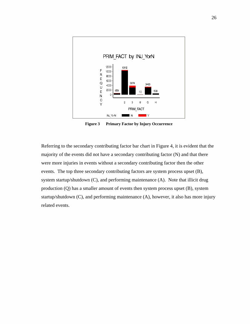
26

Figure 3 Primary Factor by Injury Occurrence

Referring to the secondary contributing factor bar chart in Figure 4, it is evident that the

majority of the events did not have a secondary contributing factor (N) and that there

were more injuries in events without a secondary contributing factor then the other

events. The top three secondary contributing factors are system process upset (B),

system startup/shutdown (C), and performing maintenance (A). Note that illicit drug

production (Q) has a smaller amount of events then system process upset (B), system

startup/shutdown (C), and performing maintenance (A), however, it also has more injury

related events.

27

Figure 4 Secondary Factor by Injury Occurrence

The industry type is another nominal variable with categorical information. In Figure 5,

the leading industry involved in fixed facility HSEES events is manufacturing (4). The

next highest number of events are from utilities (7), wholesale trade (8), transportation

(5), personal services (12), professional services (14), and illegal activity (19), but these

trail much further behind.

28

Figure 5 Industry Code by Injury Occurrence

Reviewing release types showed spills and air emissions as the types of releases that

dominated the fixed facility HSEES events. These are shown in Figure 6 and Figure 7

below. All other release types had hardly enough events to make note.

29

Figure 6 Spills by Injury Occurrence

Figure 7 Air Emissions by Injury Occurrence

6.2.2 Clustering

To cluster the data, the cause related variables were selected as input initially and the

remaining variables were added and taken away in various arrangements throughout

30

several iterations. The best discernable clusters obtained came from using primary and

secondary contributing factors, type of area the event occurred in, the industry type, and

the state. The clustering produced segments with 49.7%, 32.9%, and 17.4% of the total

events for segments 1, 2, and 3, respectively. Because the hazardous substances

subcategory variables showed no distinctness, they were replaced with the total number

of chemicals variable to summarize this finding strictly for illustration purposes. The

resulting clusters are shown in Figure 8.

Figure 8 Clustered Data

Close inspection of these segments revealed the following:

• Segment 1 shows a large number of manufacturing type events, industrial area

type events, equipment failure as the leading primary contributing factor,

31

equipment failure as the second largest contributor, and Texas as the primary

state captured in this cluster.

• Segment 2 shows about 55% of events are in a commercial area type, the

industries are fairly spread out with utilities, transportation, manufacturing, and

wholesale trade representing about half of the events, almost an equal

contribution between equipment failure and operator error as the primary factor,

and presence of a secondary factor contributing to half of segment 2 as well.

• Segment 3 has more contribution from residential area types then it does from

industrial and commercial, a little over half of the events are related to

manufacturing and illegal activities as the industry type, illegal acts are about

98.5% of the events with respect to primary contributing factors, and illicit drug

production is the leading secondary contributing factor with performing

maintenance, system startup and shutdown, and unauthorized/improper dumping

trailing behind.

• There is no difference between segments with respect to the number of chemicals

involved.

• Texas, New York, and Utah’s percent varies the most between segments. The

other states maintain a fairly even contribution across the segments.

Given the previously listed findings, one might expect the following scenarios:

• Many of the events in segment 1 occurred in Texas with the manufacturing

industry as a result of equipment failure and system/process upset.

• Many of the events in segment 2 are in a commercial with almost an equal

chance of being the result of equipment failure or operator error.

• Just less than half of the events in segment 3 are in residential areas as a result of

illegal acts, predominately illicit drug production. The methamphetamine events

are probably most prominent in this segment. The remaining half of the events

are commercial or industrial area types dealing with mostly the manufacturing

industry as a result of intentional acts. These intentional acts are related to

32

performing maintenance, system startup and shutdown, and

unauthorized/improper dumping.

Note that the clustering method does not consider the target variable. Instead, the

clustering helps describe the nature of the data content completely independent from

what is going to be predicted later in the data mining process.

6.2.3 Text Mining

Before connecting the text mining node, the data were partitioned into the following

sets: 40% training set, 30% validation set, and 30% test set. The text mining node was

set to ignore punctuation, different parts of speech, terms that appear only in a single

document, determiners (a, an, the), conjugations (and, but, or), auxiliary verbs (may, can,

should), prepositions (of, for, from), pronouns (he, it, them), participles (not, to, be),

interjections (yes, thank you, hello), and finally numbers. This greatly reduces the

number of terms to decipher, which include nouns, verbs, proper nouns, adjectives,

adverbs, and abbreviations. Finally, the text mining node was set to automatically

cluster terms and to transform the data using SVD.

After running the text miner, the interactive capability of this node allowed for a close

inspection of identified terms and their links as well as clustered terms. At this point, a

synonym list, start list, and stop list can be created. A term frequency table can be sorted

in various arrangements; a subset of documents that contain selected terms can be

filtered. This is helpful for reading groups of text descriptions with similar terms to

better understand the significance and relationship of the selected terms. Also, concept

links can be used to illustrate the links between terms.

To clean the text data, misspelled words were grouped with their correctly spelt

alternatives, abbreviations were combined with their definitions when available, and

33

other obvious synonyms were grouped together like “PRV”, “pressure relief valve”, and

“relief valve”. After all of these changes were made, the synonym list was saved.

Next, the words that appeared fewer then 3 times in total were eliminated. Any words

that describe the type of injury or the consequence of being injured or killed were also

eliminated. Eliminating these words is essential, since the end goal is to build a model

that links causes to the consequence of being injured. Other erroneous terms were

eliminated as well such as “on” and “when”. After eliminating these irrelevant terms, a

stop list was saved. The text miner was run again with the updated synonym and stop

lists.

Table 6 shows the clustered terms per segment.

Table 6 Clustered Terms per Segment

Cluster Percent Terms1 33%2 17% + result, + release, + response, + shut, + shutdown, + pressure, + fail, + company, +

failure, + unit, + line, + gas, equipment, + flare, + secure 3 8% + chemical, + mix, + police department, + laboratory, + methamphetamine, + spray,

+ treat, + explode, + home, + find, + fire department, + respond, + methamphetamine lab, + fire, + area

4 4% additional, + worker, + fume, + on-site, + expose, + area, + clean, + report, + fire department, + evacuate, + work, + out, + contain, ammonia, + time

5 29% + break, + receive, + clean up, + drum, + spill, + fire, up, into, + water, + fire department, + leak, + out, + contain, + occur, + tank

6 3% + evacuate, + build, + people working, + unknown, visiting unknown, + work, people, + measure, + visit, + decontamination, + read, emergency, + result, scene, + time

7 3% additional, + school, anhydrous ammonia, anhydrous, ammonia, + student, + fume, + eye, + valve, + respond, + expose, + police department, + laboratory, + evacuate, + tank

8 3% + expose, + wear, ppe, enforcement, + residence, + length, special agents, toxic, + affect, + action, + perform, + child, + wearing ppe, + respiratory protection, + methamphetamine lab

34

Table 7 provides a brief description of the events found in each clustered segment.

Table 7 Cluster Descriptions

Cluster Percent Description1 33% No text entries available.2 17% Contains many of equipment failure events and flare stack events3 8% Large portion of the events are related to methamphetamine labs and the remainder

dealt with general chemical releases that required the police or fire department to respond.

4 4% Contains mostly operator error events.5 29% Varying types events that do not have any obvious connections to one another.6 3% Events are mostly associated with each other by the word evacuate. However, there

are a large number of events that stated "no evacuation".7 3% Mostly ammonia and school related events.8 3% Events are mostly associated with methamphetamine events and the use of PPE.

A Segment Profile node illustrates the clustered terms distributions as they relate to input

variables. Events within each segment are depicted by either concentric rings for

categorical input variables or bar charts for interval variables. The outer circle of the

concentric ring shows the distribution of the attributes within each segment, and the

inner ring shows the distribution of the same attributes within the entire population of

data. In the bar charts, the solid bars represent the events in the segment and the hollow

outlined bars represent the population. Although we want segments distinct from one

another, the distribution of the attributes within each segment should be similar to the

distribution of the attributes within the population.

35

Figure 9 is a snapshot of the cluster results for each segment.

Figure 9 Cluster Rings

The segments are listed by the number of events they contain in decreasing order. The

input variables are depicted in decreasing order of their worth. The following

observations were made based on the concentric ring illustration:

• Segment 1 events represent the industry types similarly to the entire population

of events, but the segment events lack 5 industries. The secondary factors are

also fairly well represented in the segment with some variations. Air emission

and spill releases as well as the mixture substance subcategory are similar

between the population (hollow outlined bars) and the segment (solid bars).

Finally, the primary factor is similar in distribution between the population and

36

segment events. This segment contains the events with no text entries, so there is

no text-based theme for this segment to compare to the population.

• Segment 5 represents the secondary factor distribution almost exactly like the

population. The industry codes are also well represented in this segment, but the

air emission and spill releases do not perform as well. This segment is an

assortment of different types of events, so it is difficult to compare the text-based

theme of the segment with the population.

• Segment 2 represents the industry type distribution similarly to the population,

but the larger amount of wholesale trade industry represented in the segment.

The other inorganic substances subcategory representation in the segment

compared to the population is acceptable, and so are the secondary and primary

contributing factors, the air emission releases, and the volatile organic compound

subcategory. The text comments described equipment failure and flare stack

release events and this is consistent with the concentric rings showing a large

proportion of manufacturing events with equipment failure as the primary factor.

The similarities between the segment and population with regard to air emission

releases can be attributed to the large number of flare stack events contained in

this segment.

• Segments 3, 4, 6, 7, and 8 all do poorly with representation of the population.

This is expected because these segments have a small number of events. Recall

that segment 3 contains events that describe methamphetamine labs and other

types of labs where chemicals were released. Reviewing the concentric rings for

secondary contributing factors shows a larger portion of illicit drug production

then any of the other segments as well as a larger portion of illegal activity as the

industry type.

The results of the text mining node that is passed on to the modeling nodes are 36 SVD

vector inputs.

37

6.3 Model

To model the HSEES data, two different types of models were applied—the decision

tree and the logistic regression. These models were run with various arrangements of the

cause related variable inputs to maximize its predicting power, and then a separate set of

decision tree and logistic regression models were run that included both the cause related

variables and the text SVD inputs. The comparison of both sets of models will help

delineate the value added by the text data.

6.3.1 Decision Tree without Text Input

The decision tree node was connected directly to the partition node and the cause related

variables were set to input, occurrence of injuries set to target, and all other variables set

to reject. The decision tree node was adjusted multiple times to optimize the accuracy of

the model. Table 8 contains the event classification table.

Table 8 Classifications for Decision Tree with No Text Input

Data FALSE TRUE FALSE TRUERole Target Negative Negative Positive Positive

TRAIN INJ_YorN 534 6,994 34 103 VALIDATE INJ_YorN 409 5,225 47 68

TRAIN INJ_YorN 6.97% 91.25% 0.44% 1.34%VALIDATE INJ_YorN 7.11% 90.89% 0.82% 1.18%

Frequencies

Percent of Total

In the event classification table, “FALSE Negative” refers to the predicted outcome of

injuries = no when it should have been injuries = yes. Similarly, “TRUE Negative” is

the number of events the model correctly predicts as injuries = no, “FALSE Positive” is

the number of events the model predicts as injuries = yes when it should have been

38

injuries = no, and finally “TRUE Positive” is the number of events correctly predicted as

injury = yes. For this decision tree, it correctly predicted 1.34% injuries, but incorrectly

predicted no injuries for the other 6.97% of events that had injuries. In other words, it

correctly predicted 16% of the injury events.

Table 9 contains the variable importance table. NRULES is the number of times the

variable appears in a node, IMPORTANCE shows the level of importance for the

variable in the training dataset, and VIMPORTANCE shows the level of importance for

the variable in the validation dataset. RATIO is the IMPORTANCE divided by the

VIMPORTANCE. In this table, it is clear that the industry code has equal importance

across the two sets, air emission releases have absolutely no importance with relation to

the validation set, and the remaining release types and chemical subcategories do not

have much importance in either dataset.

Table 9 Variable Importance for Decision Tree with No Text Input

Obs NAME NRULES IMPORTANCE VIMPORTANCE RATIO1 NIND_CODE 1 1.000 1.000 1.0002 SEC_FACT 3 0.693 0.662 0.9553 REL_AIREMIS 1 0.404 0.000 0.0004 PRIM_FACT 3 0.372 0.400 1.0735 SC_OISC 2 0.269 0.310 1.1536 SC_AMMONIA 3 0.235 0.214 0.9117 SC_ACID 3 0.222 0.250 1.1278 SC_OXYORG 1 0.220 0.160 0.7309 REL_SPILL 2 0.183 0.081 0.443

10 SC_MIX 1 0.180 0.159 0.88211 SC_OTHER 1 0.114 0.084 0.73812 SC_CHORLINE 2 0.107 0.111 1.03713 REL_FIRE 1 0.107 0.070 0.659

39

An example rule produced by this decision tree is:

• If the primary factor is something other than Human Error,

o AND the secondary contributing factors are system/process upset or

power failure/electrical problems

o AND industry type is manufacturing or mining, then

Occurrence of injuries is estimated to be 0.1% for 1,902 events.

Take this same set of rules except consider the scenario where there is at least one acid

present, then the occurrence of injuries jumps to 5.9% for 17 events. This percentage

increase makes sense because the presence of an acid is adding a hazard to the scenario.

Looking at the leaf nodes with large percent estimations for injuries = yes can help

identify the main scenarios that cause injuries. Branches with higher percent predictions

for injuries also contain few events, which is intuitive since only a small percentage of

the total events result in injury. In addition, the predicted percentages for injuries

between the training and validation set differ significantly more for smaller groupings of

events. Thus, a more qualitative approach was taken to identify key components for

these high injury yielding events.

• Explosions in the utilities or transportation industries is expected to have 53.8%

occurrence of injuries in 13 events for the training set and 35.3% occurrence of

injuries in 17 events for the validation set.

• Illicit drug production or improper mixing in the utilities or transportation

industries is predicted to have 22.5% occurrence of injuries in 111 events and

13.8% occurrence of injuries in 87 events in the training and validation datasets,

respectively.

• The presence of at least one hazardous substance mixture in an event that

involves improper mixing or performing maintenance and is in the professional

services or illegal activity industries is expected to have 75.6% occurrence of

injuries in 41 events and 65.1% occurrence of injuries in 43 events for the

40

training and validation datasets, respectively. These events account for many

methamphetamine related events.

• The presence of at least 1 ammonia substance, released via air emission due to

operator error in the utilities or transportation industries is expected to have

100% occurrence of injuries in 13 events and 88.9% occurrence of injuries in 9

events for the training and validation datasets, respectively. Events where a tank

of ammonia is accidentally spilled fits this scenario description well.

• The presence of at least 1 acid, released via air emission due to operator error in

the utilities or transportation industries is expected to have 82.6% occurrence of

injuries in 23 events and 73.7% occurrence of injuries in 19 events for the

training and validation datasets, respectively.

6.3.2 Decision Tree with Text Input

A second decision tree node was connected to the text miner node and the settings were

set identically to the decision tree discussed in section 6.3.1. The cause related variables

and the SVD variables from the text mining node were set as input, occurrence of

injuries was set as the target, and all other variables were set to reject.

Table 10 on the following page contains the event classification table.

41

Table 10 Classifications for Decision Tree with Text Input

Data FALSE TRUE FALSE TRUERole Target Negative Negative Positive Positive

TRAIN INJ_YorN 271 6,918 110 366 VALIDATE INJ_YorN 264 5,117 155 213

TRAIN INJ_YorN 3.54% 90.25% 1.44% 4.77%VALIDATE INJ_YorN 4.59% 89.01% 2.70% 3.70%

Frequencies

Percent of Total

The decision tree with the incorporated SVD vectors from the text node classified the

events much better then the decision tree without the SVD vectors. Table 10 shows the

decision tree with SVD input correctly predicted 4.79% injuries, but incorrectly

predicted no injuries for the other 3.52% of events that had injuries. This translates to

correct predictions for 57% of the injury events, a sizeable improvement from the

decision tree model without the text input.

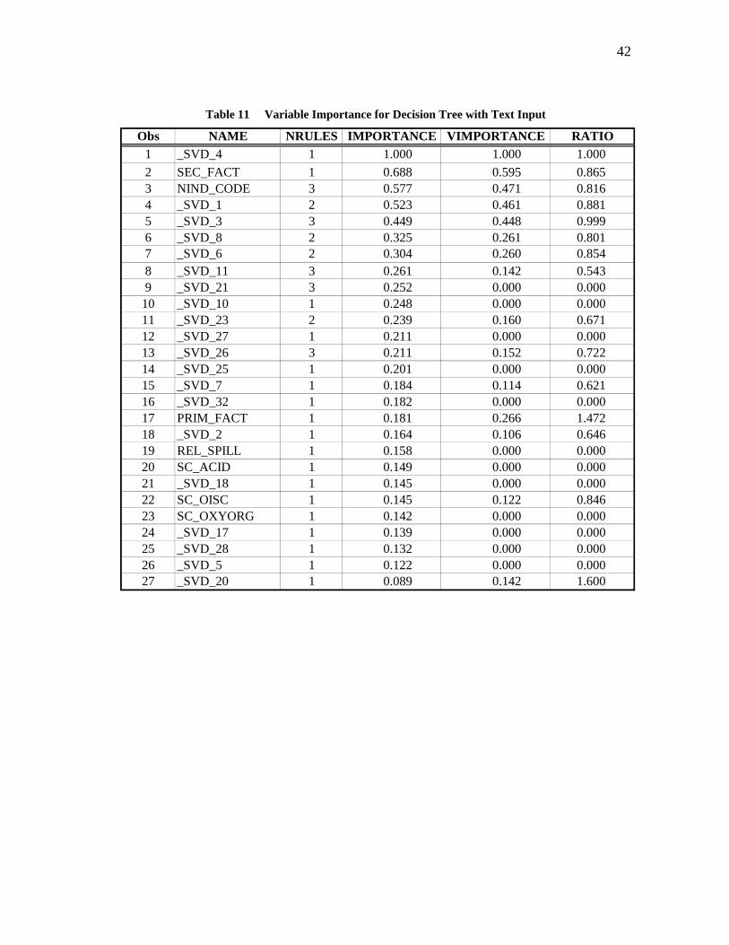
Table 11 contains the variable importance table. In this table, it is clear that the _SVD_4

vector has equal importance across the training and validation datasets, the secondary

contributing factors have about 0.6 importance, and the industry type and _SVD_1

vector have about 0.5 importance across the training and validation datasets.

42

Table 11 Variable Importance for Decision Tree with Text Input

Obs NAME NRULES IMPORTANCE VIMPORTANCE RATIO1 _SVD_4 1 1.000 1.000 1.0002 SEC_FACT 1 0.688 0.595 0.8653 NIND_CODE 3 0.577 0.471 0.8164 _SVD_1 2 0.523 0.461 0.8815 _SVD_3 3 0.449 0.448 0.9996 _SVD_8 2 0.325 0.261 0.8017 _SVD_6 2 0.304 0.260 0.8548 _SVD_11 3 0.261 0.142 0.5439 _SVD_21 3 0.252 0.000 0.000

10 _SVD_10 1 0.248 0.000 0.00011 _SVD_23 2 0.239 0.160 0.67112 _SVD_27 1 0.211 0.000 0.00013 _SVD_26 3 0.211 0.152 0.72214 _SVD_25 1 0.201 0.000 0.00015 _SVD_7 1 0.184 0.114 0.62116 _SVD_32 1 0.182 0.000 0.00017 PRIM_FACT 1 0.181 0.266 1.47218 _SVD_2 1 0.164 0.106 0.64619 REL_SPILL 1 0.158 0.000 0.00020 SC_ACID 1 0.149 0.000 0.00021 _SVD_18 1 0.145 0.000 0.00022 SC_OISC 1 0.145 0.122 0.84623 SC_OXYORG 1 0.142 0.000 0.00024 _SVD_17 1 0.139 0.000 0.00025 _SVD_28 1 0.132 0.000 0.00026 _SVD_5 1 0.122 0.000 0.00027 _SVD_20 1 0.089 0.142 1.600

43

The weights per cluster segment for SVD_1 and SVD_4 are provided in Table 12 below.

The percents are the portion of events per cluster.

Table 12 Cluster Weights for SVD_1 and SVD_4

Cluster Percent _SVD_1 _SVD_41 33% 0.000 0.0002 17% 0.187 -0.0773 8% 0.241 -0.0634 4% 0.645 -0.0915 29% 0.235 -0.0966 3% 0.216 -0.1077 3% 0.182 0.0828 3% 0.184 -0.096

Compared to the other SVD vectors (not shown), SVD_1 has the highest weights across

the largest number of clusters. This is a result of SVD_1 accounting for most of the

variability in the model. Clusters 2, 3, 5, 6, 7, and 8 are all weighted about 0.2 and the

clusters include various types of events that are not generally related to operator error.

Cluster 4 has the largest weight of 0.65 and only accounts for 4% of the events; cluster 4

contains mainly operator error events. The weight for cluster 1 is 0 since this cluster

represents the set of events with no text entries. The vector SVD_4 has equal weights of

about -0.1 for clusters 2-6 and 8. Cluster 7 is weighted as 0.1 and contains ammonia and

school related events. Because the clusters are not very distinct from one another,

interpretation of the scenarios in the decision tree is limited, and drawing meaningful

conclusions from these events is limited as well.

The low event number and high percent predicted injury occurrence scenarios were

reviewed and the following are some of the findings:

• Events where the primary contributing factor is operator error and the secondary

factor is either improper mixing or performing maintenance with events weighted

44

< 0.00413 in SVD_4 are predicted to result in 57.6% occurrence of injuries in

110 events and 51.8% occurrence of injuries in 85 events for the training and

validation datasets, respectively.

o This scenario is describing events where the operator erred via improper

mixing or performing maintenance and events that are not grouped in

cluster 7.

• Events where fire or illicit drug production were the secondary contributing

factors with weights < 0.00413 in SVD_4 are predicted to result in 17.7%

occurrence of injuries in 844 events and 15.8% occurrence of injuries in 659

events for the training and validation sets, respectively.

o This scenario is describing events that are most likely coming from

cluster 3, 4, or 5 which contain the clustered word “fire”. Cluster 3

contains events with explosions from methamphetamine labs.

• Events in the wholesale trade or professional services industry with weights

between 0.00413 and 0.10328 for SVD_4 are predicted to have 52.0%

occurrence of injuries in 102 events and 58.5% occurrence of injuries in 65

events for the training and validation sets, respectively.

o The events in this scenario are singled out to cluster 7 which is described

as mostly ammonia and school-related events. The wholesale trade

industry has a large number of events with ammonia releases and the

professional services industry has a large number of school services

(elementary school, colleges and universities, etc.) grouped with it.

6.3.3 Logistic Regression Node without Text Input

A few iterations were required to build the best possible logistic regression model with

the cause related predictor variables. The final setup for this model includes industry

type, release types, primary and secondary contributing factors set to input, occurrence

45

of injuries set to target, and all other variables set to reject. The model selection of

choice is stepwise regression.

Table 13 shows the event classification table. The logistic regression model correctly

predicted 1.72% injuries, but incorrectly predicted no injuries for the other 6.59% of

events that had injuries. Similarly stated, this decision tree model correctly predicted

21% of the injury events.

Table 13 Classifications for Logistic Regression with No Text Input

Data FALSE TRUE FALSE TRUERole Target Negative Negative Positive Positive

TRAIN INJ_YorN 505 6,939 89 132 VALIDATE INJ_YorN 368 5,174 98 109

TRAIN INJ_YorN 6.59% 90.53% 1.16% 1.72%VALIDATE INJ_YorN 6.40% 90.00% 1.70% 1.90%

Frequencies

Percent of Total

Table 14 on the following page lists the parameter estimate results for the selected

variables.

46

Table 14 Maximum Likelihood Estimates for Logistic Regression without Text

Parameter INJ YorN Category DF Estimate Standard

ErrorWald Chi-

SquarePr >

ChiSqStandardized

Estimate Exp(Est)

Intercept Y 1 -3.1579 2.5627 1.52 0.2178 0.043NIND_CODE Y 1 1 -0.2421 0.3355 0.52 0.4704 0.785NIND_CODE Y 2 1 -2.3574 0.9511 6.14 0.0132 0.095NIND_CODE Y 3 1 -0.0246 0.2863 0.01 0.9314 0.976NIND_CODE Y 4 1 -1.0436 0.1513 47.56 <.0001 0.352NIND_CODE Y 5 1 -1.073 0.2803 14.65 0.0001 0.342NIND_CODE Y 6 1 0.4252 1.033 0.17 0.6807 1.53NIND_CODE Y 7 1 -0.7176 0.2238 10.28 0.0013 0.488NIND_CODE Y 8 1 -0.6896 0.2755 6.26 0.0123 0.502NIND_CODE Y 9 1 1.0625 0.2327 20.85 <.0001 2.894NIND_CODE Y 10 1 0.5574 0.3805 2.15 0.143 1.746NIND_CODE Y 11 1 0.3295 0.3662 0.81 0.3682 1.39NIND_CODE Y 12 1 0.6858 0.1683 16.61 <.0001 1.985NIND_CODE Y 13 1 0.3664 0.4045 0.82 0.365 1.443NIND_CODE Y 14 1 1.0046 0.1842 29.75 <.0001 2.731NIND_CODE Y 15 1 -0.0418 0.3574 0.01 0.907 0.959NIND_CODE Y 16 1 -0.3209 0.5403 0.35 0.5525 0.725NIND_CODE Y 17 1 1.3005 0.3566 13.3 0.0003 3.671NIND_CODE Y 18 1 1.0943 0.4605 5.65 0.0175 2.987NIND_CODE Y 19 1 -0.1151 0.2544 0.2 0.651 0.891PRIM_FACT Y 2 1 -0.4992 0.1645 9.21 0.0024 0.607PRIM_FACT Y 3 1 0.7239 0.1591 20.7 <.0001 2.062PRIM_FACT Y 8 1 0.5335 0.4222 1.6 0.2064 1.705PRIM_FACT Y G 1 -0.6747 0.2107 10.25 0.0014 0.509REL_AIREMIS Y 1 0.3838 0.0735 27.28 <.0001 0.1524 1.468SC_ACID Y 1 0.6764 0.1281 27.87 <.0001 0.1226 1.967SC_AMMONIA Y 1 0.6665 0.1625 16.83 <.0001 0.0963 1.947SC_BASES Y 1 0.5161 0.2107 6 0.0143 0.0533 1.676SC_CHORLINE Y 1 0.8852 0.2134 17.21 <.0001 0.0841 2.424SC_OISC Y 1 -0.6551 0.0976 45.05 <.0001 -0.2708 0.519SC_OTHER Y 1 0.385 0.1368 7.92 0.0049 0.0642 1.47SC_OXYORG Y 1 0.3609 0.1071 11.35 0.0008 0.0873 1.435SEC_FACT Y 1 1 2.3502 2.5676 0.84 0.36 10.488SEC_FACT Y 2 1 0.0123 2.5727 0 0.9962 1.012SEC_FACT Y 3 1 1.9573 2.575 0.58 0.4472 7.08SEC_FACT Y 4 1 0.1735 2.5675 0 0.9461 1.189SEC_FACT Y 8 1 1.3584 2.5712 0.28 0.5973 3.89SEC_FACT Y A 1 0.7002 2.5668 0.07 0.785 2.014SEC_FACT Y B 1 -0.8022 2.5887 0.1 0.7567 0.448SEC_FACT Y C 1 -0.5688 2.5951 0.05 0.8265 0.566SEC_FACT Y E 1 -5.4724 7.9975 0.47 0.4938 0.004SEC_FACT Y F 1 -0.2557 2.577 0.01 0.9209 0.774SEC_FACT Y I 1 0.00208 2.74 0 0.9994 1.002SEC_FACT Y J 1 1.4371 2.5666 0.31 0.5755 4.209SEC_FACT Y K 1 3.3018 2.5814 1.64 0.2009 27.163SEC_FACT Y L 1 1.5423 2.5739 0.36 0.549 4.675SEC_FACT Y N 1 0.8416 2.5592 0.11 0.7423 2.32SEC_FACT Y O 1 -7.2505 45.3653 0.03 0.873 0.001SEC_FACT Y P 1 0.1933 2.7746 0 0.9445 1.213SEC_FACT Y Q 1 1.7903 2.5715 0.48 0.4863 5.991

47

Recall that logistic regression builds a model that predicts the likelihood of some

response via odds ratio. The “Estimate” column gives the estimated coefficient for each

variable. For interval variables such as air emission release type, the coefficient will be

multiplied by the number of air emission releases. For categorical variables such as

industry type, the model splits these into binary variables of industry code 17, industry

code 18, and so on such that if NIND_CODE 17 = Yes, the value 1 will be multiplied by

the coefficient.

Using the coefficient estimates from Table 14, the equation for this model is:

===== )Pr(/)ln[Pr()](ln[ NoInjuryYesInjuryYesInjuryOddsRatio

LL ++++− AIREMISRELCODENINDCODENIND _*4.018_*3.117_*2.3

If there is an event involving illegal activity (industry type 18), then NIND_CODE 18 =

1 else it is 0. The other categorical variables are treated the same way. If there are 3

substances that were released via air emission, then REL_AIREMIS = 3. The other

interval variables are treated similarly. The final results gives the odds ratio, which

describes how much more likely it is for an injury to occur then for an injury not to

occur. The equation can be manipulated to solve for Pr(Injury=Yes).

Note that the statistical significance of the variables should be considered in terms of

identifying the more important factors. Looking at the coefficients alone does not give

an adequate assessment of the variable significance since the order of magnitude among

the variables is different. Reviewing the odds ratio in the column “Exp(est)” can give a

good indication of what variables have a larger effect on the occurrence of injury.

Considering both the odds ratio and the p-values found in column “Pr > ChiSq” helps

discern which variables affect the occurrence of an injury and are still statistically

significant. The variables with p-values less than 0.05 were filtered out and ranked in

decreasing order by their odds ratio estimate. The results are given in Table 15.

48

Table 15 Reduced Variable List for Logistic Regression with No Text Input

Parameter Category Category Description Estimate Standard Error

Wald Chi-

Square

Pr > ChiSq

Standardized Estimate Exp(Est)

NIND_CODE 17 Private vehicle or property 1.3005 0.3566 13.3 0.0003 3.671NIND_CODE 18 Illegal activity (non-drug related) 1.0943 0.4605 5.65 0.0175 2.987NIND_CODE 9 Retail trade 1.0625 0.2327 20.85 <.0001 2.894NIND_CODE 14 Professional services 1.0046 0.1842 29.75 <.0001 2.731SC_CHORLINE 0.8852 0.2134 17.21 <.0001 0.0841 2.424PRIM_FACT 3 Operator error 0.7239 0.1591 20.7 <.0001 2.062NIND_CODE 12 Personal services 0.6858 0.1683 16.61 <.0001 1.985SC_ACID 0.6764 0.1281 27.87 <.0001 0.1226 1.967SC_AMMONIA 0.6665 0.1625 16.83 <.0001 0.0963 1.947SC_BASES 0.5161 0.2107 6 0.0143 0.0533 1.676SC_OTHER 0.385 0.1368 7.92 0.0049 0.0642 1.47REL_AIREMIS 0.3838 0.0735 27.28 <.0001 0.1524 1.468SC_OXYORG 0.3609 0.1071 11.35 0.0008 0.0873 1.435PRIM_FACT 2 Equipment failure -0.4992 0.1645 9.21 0.0024 0.607SC_OISC -0.6551 0.0976 45.05 <.0001 -0.2708 0.519PRIM_FACT G Intentional act -0.6747 0.2107 10.25 0.0014 0.509NIND_CODE 8 Wholesale trade -0.6896 0.2755 6.26 0.0123 0.502NIND_CODE 7 Utilities -0.7176 0.2238 10.28 0.0013 0.488NIND_CODE 4 Manufacturing -1.0436 0.1513 47.56 <.0001 0.352NIND_CODE 5 Transportation -1.073 0.2803 14.65 0.0001 0.342NIND_CODE 2 Mining -2.3574 0.9511 6.14 0.0132 0.095 The following observations are made based on these results:

• None of the secondary contributing factors were considered statistically

significant.

• A private vehicle or property related event is 3.7 times more likely to result in an

injury.

• Events related to illegal activity that is non-drug related, retail trade, and

professional service industries all are roughly 3 times more likely to have an

injury.

• Chlorine events are 2.5 times more likely to result in an injury whereas acid,

ammonia, and base events are only 2 times more likely to result in an injury.

Substances in the oxy-organic and other substances categories are only about 1.5

times more likely to result in an injury. Interestingly enough, the presence of

49

substances in the other inorganic substances category are 2 times more likely to

NOT result in an injury.

• The only statistically significant release type is air emissions, which has the odds

of 3 to 1 that a person will be injured.

• Events caused by operator error have 2 to 1 odds that someone will be injured,

but events caused by equipment failure and intentional act are respectively 1.6

and 2.0 times more likely NOT to result in an injury.

• Events in the wholesale trade and utilities industries are 2.0 times more likely to

NOT result in injury and events in the manufacturing and transportation

industries are showing respectively 2.8 and 2.9 times the likelihood of resulting

in an injury. Mining industry events are showing the occurrence of an injury is

10 times less likely.

Based on this logistic regression model, efforts to decrease the occurrence of injuries can

be focused on the private frontier, illegal activities, retail trades, and professional

services. Data inspection of these industry types revealed the following:

• Illegal activities as events dealing with disgruntled employees, vandalism, and

domestic disputes.

• Retail trade events dealt primarily with ammonia releases/leaks, improper mixing

of chemicals, use of pesticides without proper ventilation, or other substance

leaks. Many of the events with ammonia leaks were related to someone stealing

the ammonia to make methamphetamines and not completely shutting the valves.

• Professional services events typically dealt with broken thermometers or

accidentally spilling materials.

• Personal services industry included many meth lab related events where

surrounding households had to be evacuated.

An effective way to reduce injuries is something ATSDR and participating states are

already doing—focusing on outreach programs to educate people about hazards

associated with substances such as mercury, chlorine, and pesticides. Another

50

suggestion to reduce the opportunity for injuries with respect to thieves stealing

ammonia is to collaborate with retail trades to identify and implement ways of storing

their chemicals in a more secure location.

6.3.4 Logistic Regression Node with Text Input

A few iterations were required to build the best possible logistic regression model with

the cause related predictor variables and SVD variables. The final setup for this model

includes industry type, release types, primary and secondary contributing factors set to

input, occurrence of injuries set to target, and all other variables set to reject. The model

selection of choice is stepwise regression.

Table 16 shows the event classifications and Table 17 lists the parameter estimate

results. The logistic regression with SVD input correctly predicted 3.65% injuries, but

incorrectly predicted no injuries for the other 4.66% of events that had injuries.

Table 16 Classifications for Logistic Regression with Text Input

Data FALSE TRUE FALSE TRUERole Target Negative Negative Positive Positive

TRAIN INJ_YorN 357 6,935 93 280 VALIDATE INJ_YorN 239 5,186 86 238

TRAIN INJ_YorN 4.66% 90.48% 1.21% 3.65%VALIDATE INJ_YorN 4.16% 90.21% 1.50% 4.14%

Frequencies

Percent of Total

51

Table 17 Maximum Likelihood Estimates for Logistic Regression with Text

Parameter INJ YorN Category DF Estimate Standard

ErrorWald Chi-

SquarePr >

ChiSqStandardized

Estimate Exp(Est)

Intercept Y 1 -3.1579 2.5627 1.52 0.2178 0.043NIND_CODE Y 1 1 -0.2421 0.3355 0.52 0.4704 0.785NIND_CODE Y 2 1 -2.3574 0.9511 6.14 0.0132 0.095NIND_CODE Y 3 1 -0.0246 0.2863 0.01 0.9314 0.976NIND_CODE Y 4 1 -1.0436 0.1513 47.56 <.0001 0.352NIND_CODE Y 5 1 -1.073 0.2803 14.65 0.0001 0.342NIND_CODE Y 6 1 0.4252 1.033 0.17 0.6807 1.53NIND_CODE Y 7 1 -0.7176 0.2238 10.28 0.0013 0.488NIND_CODE Y 8 1 -0.6896 0.2755 6.26 0.0123 0.502NIND_CODE Y 9 1 1.0625 0.2327 20.85 <.0001 2.894NIND_CODE Y 10 1 0.5574 0.3805 2.15 0.143 1.746NIND_CODE Y 11 1 0.3295 0.3662 0.81 0.3682 1.39NIND_CODE Y 12 1 0.6858 0.1683 16.61 <.0001 1.985NIND_CODE Y 13 1 0.3664 0.4045 0.82 0.365 1.443NIND_CODE Y 14 1 1.0046 0.1842 29.75 <.0001 2.731NIND_CODE Y 15 1 -0.0418 0.3574 0.01 0.907 0.959NIND_CODE Y 16 1 -0.3209 0.5403 0.35 0.5525 0.725NIND_CODE Y 17 1 1.3005 0.3566 13.3 0.0003 3.671NIND_CODE Y 18 1 1.0943 0.4605 5.65 0.0175 2.987NIND_CODE Y 19 1 -0.1151 0.2544 0.2 0.651 0.891PRIM_FACT Y 2 1 -0.4992 0.1645 9.21 0.0024 0.607PRIM_FACT Y 3 1 0.7239 0.1591 20.7 <.0001 2.062PRIM_FACT Y 8 1 0.5335 0.4222 1.6 0.2064 1.705PRIM_FACT Y G 1 -0.6747 0.2107 10.25 0.0014 0.509REL_AIREMIS Y 1 0.3838 0.0735 27.28 <.0001 0.1524 1.468SC_ACID Y 1 0.6764 0.1281 27.87 <.0001 0.1226 1.967SC_AMMONIA Y 1 0.6665 0.1625 16.83 <.0001 0.0963 1.947SC_BASES Y 1 0.5161 0.2107 6 0.0143 0.0533 1.676SC_CHORLINE Y 1 0.8852 0.2134 17.21 <.0001 0.0841 2.424SC_OISC Y 1 -0.6551 0.0976 45.05 <.0001 -0.2708 0.519SC_OTHER Y 1 0.385 0.1368 7.92 0.0049 0.0642 1.47SC_OXYORG Y 1 0.3609 0.1071 11.35 0.0008 0.0873 1.435SEC_FACT Y 1 1 2.3502 2.5676 0.84 0.36 10.488SEC_FACT Y 2 1 0.0123 2.5727 0 0.9962 1.012SEC_FACT Y 3 1 1.9573 2.575 0.58 0.4472 7.08SEC_FACT Y 4 1 0.1735 2.5675 0 0.9461 1.189SEC_FACT Y 8 1 1.3584 2.5712 0.28 0.5973 3.89SEC_FACT Y A 1 0.7002 2.5668 0.07 0.785 2.014SEC_FACT Y B 1 -0.8022 2.5887 0.1 0.7567 0.448SEC_FACT Y C 1 -0.5688 2.5951 0.05 0.8265 0.566SEC_FACT Y E 1 -5.4724 7.9975 0.47 0.4938 0.004SEC_FACT Y F 1 -0.2557 2.577 0.01 0.9209 0.774SEC_FACT Y I 1 0.00208 2.74 0 0.9994 1.002SEC_FACT Y J 1 1.4371 2.5666 0.31 0.5755 4.209SEC_FACT Y K 1 3.3018 2.5814 1.64 0.2009 27.163SEC_FACT Y L 1 1.5423 2.5739 0.36 0.549 4.675SEC_FACT Y N 1 0.8416 2.5592 0.11 0.7423 2.32SEC_FACT Y O 1 -7.2505 45.3653 0.03 0.873 0.001SEC_FACT Y P 1 0.1933 2.7746 0 0.9445 1.213SEC_FACT Y Q 1 1.7903 2.5715 0.48 0.4863 5.991

52

Both the odds ratio and the p-values found in column “Pr > ChiSq” were used to discern

which variables affect the occurrence of an injury and are still statistically significant.

The variables with p-values less than 0.05 were filtered out and ranked in decreasing

order by their odds ratio estimate. The results are given in Table 18.

Table 18 Reduced Variable List for Logistic Regression with Text Input

Parameter Category Category Description Estimate Standard Error

Wald Chi-

Square

Pr > ChiSq

Standardized Estimate Exp(Est)

_SVD_4 5.9036 0.4387 181.09 <.0001 0.3314 366.372_SVD_1 5.6878 0.378 226.45 <.0001 0.486 295.234_SVD_11 2.3812 0.4042 34.7 <.0001 0.1506 10.818SEC_FACT K Explosion 2.2691 1.112 4.16 0.0413 9.671_SVD_25 2.1992 0.5262 17.47 <.0001 0.1398 9.018_SVD_24 2.0997 0.4458 22.19 <.0001 0.1593 8.164_SVD_20 1.8752 0.4127 20.65 <.0001 0.1507 6.522_SVD_23 1.6062 0.4209 14.56 0.0001 0.1774 4.984NIND_CODE 17 Private vehicle or property 1.5191 0.3991 14.49 0.0001 4.568_SVD_6 1.3335 0.4397 9.2 0.0024 0.0645 3.794_SVD_29 1.0776 0.4578 5.54 0.0186 0.0643 2.938SC_CHORLINE 1.0645 0.2409 19.53 <.0001 0.1011 2.9_SVD_10 1.0116 0.3533 8.2 0.0042 0.0963 2.75NIND_CODE 14 Professional services 0.877 0.2237 15.36 <.0001 2.404_SVD_9 0.8092 0.3817 4.5 0.034 0.055 2.246SC_AMMONIA 0.8093 0.1849 19.15 <.0001 0.117 2.246NIND_CODE 9 Retail trade 0.7375 0.284 6.75 0.0094 2.091PRIM_FACT 3 Operator error 0.5119 0.1868 7.51 0.0061 1.668NIND_CODE 12 Personal services 0.5085 0.201 6.4 0.0114 1.663REL_FIRE 0.4024 0.1546 6.77 0.0093 0.0453 1.495REL_AIREMIS 0.3282 0.0884 13.78 0.0002 0.1304 1.388PRIM_FACT 2 Equipment failure -0.4227 0.1931 4.79 0.0286 0.655PRIM_FACT G Intentional act -0.5836 0.2345 6.19 0.0128 0.558NIND_CODE 5 Transportation -0.6431 0.3235 3.95 0.0468 0.526NIND_CODE 4 Manufacturing -0.6691 0.1776 14.2 0.0002 0.512_SVD_31 -1.2139 0.5183 5.48 0.0192 -0.072 0.297_SVD_17 -1.2473 0.4199 8.82 0.003 -0.1072 0.287_SVD_15 -1.7313 0.4306 16.17 <.0001 -0.0975 0.177_SVD_2 -2.5201 0.3756 45.01 <.0001 -0.1857 0.08NIND_CODE 2 Mining -2.7277 1.2407 4.83 0.0279 0.065Intercept -3.6029 1.057 11.62 0.0007 0.027 There are 15 SVD vectors that show statistical significance, 11 of which have odds ratios

larger than 2.2 with a maximum of 366. The weights were reviewed for each of the 15

53

SVD vectors and no discernable conclusions could be drawn because clustered events

and terms are not distinct enough.

The following observations are made based on these results:

• Only one secondary contributing factor (Explosion) was determined statistically

significant.

• A private vehicle or property related event is 4.6 times more likely to result in an

injury.

• Professional service events are 2.4 times more likely to result in injuries.

• Events related to retail trade, operator error, and personal services industries all

are roughly 2 times more likely to have an injury.

• Chlorine events are 2.9 times more likely to result in an injury whereas ammonia

events are only 2.2 times more likely to result in an injury.

• The only statistically significant release types are air emissions and fire, which

are 1.5 and 1.4 times more likely to result in injury, respectively.

• Events caused by equipment failure and intentional act are respectively 1.6 and

2.0 times more likely NOT to result in an injury.

• Events in the transportation and manufacturing industries are 2.0 times more

likely to NOT result in injury. Mining industry events are showing the

occurrence of an injury is 37 times less likely.

Based on the listed findings, similar conclusions to the non-text logistic regression

model results can be drawn. Note that the logistic regression model with text input did

identify explosions as a statistically significant event.

6.4 Assess

Finally, the model comparison node was connected to the two regression nodes. The

accuracy of the regression models were compared by applying the models to all data

subsets (train, validate, and test). The logistic regression model with the text input was

54

determined to predict injury occurrences the best as can be seen by the higher lift in each

dataset. Cumulative lift charts for the train, validate, and test sets are provided in Figure

10, Figure 11, and Figure 12, respectively. The lift in all three datasets is similar

showing the models performed consistently.

Figure 10 Cumulative Lift Comparison for Train Dataset

Figure 11 Cumulative Lift Comparison for Validate Dataset

55

Figure 12 Cumulative Lift Comparison for Test Dataset

56

7. CONCLUSIONS AND RECOMMENDATIONS

The conclusions and recommendations for this research are presented in this section.

7.1 Conclusions

Data mining proved to be beneficial in both describing the HSEES events and building a

fairly good model to predict the occurrence of injuries. The following are some

conclusions drawn based on the analysis:

• Although HSEES data is collected to describe the effects hazardous substance

releases/threatened releases have on people, a fairly good predictive model was

still obtained from the few variables identified as cause related.

• Visually exploring the data via bar graphs did not yield any noticeable patterns.

• Clustering the data identified groupings of categories across the variable inputs

such as manufacturing events resulting from intentional acts such as system

startup and shutdown, performing maintenance, and improper dumping.

• Text mining the data allowed for clustering the events and further description of

the data, however, these events were not noticeably distinct and drawing

conclusions based on these clusters was limited.

• Inclusion of the text comments to the overall analysis of HSEES data greatly

improved the predictive power of the models. Interpretation of the textual data’s

contribution was limited, however, the qualitative conclusions drawn were

similar to the model without textual data input.

Probably the most beneficial part of performing a data mining analysis on the HSEES

data is having the capability to relate characteristics across several variable types to one

another. Annual reports provided by ATSDR do not go into such detail—the annual

reports describe the number of occurrences and percent distributions of event

characteristics with some associations made to other variable types. For example, in the

57

2004 report, the percent of events with victims with respect to the number of substances

present from a single category or more than one category was determined [7]. The data

mining analysis was able to address questions with regard to types of events that occur

without having to read individual data entries.

7.2 Recommendations

This study focused on identifying causal factors that result in injury, however, there are

other potential studies that would be beneficial to explore such as:

• Use data mining techniques to describe the victim data.

• Translate the chemical quantities into a common unit, compare the quantities of

each substance type to their corresponding permissible exposure limits (PEL)

defined by OSHA, and incorporate these data into an analysis such that the

consequence severity can be assessed.

• Use link analysis to build association rules for text comment entries and

determine if there are any strong cause-consequence associations.

• Try different approaches to build more distinct clusters within the textual data

such that more interpretable conclusions may be drawn.

58

REFERENCES

[1] S. Anand, N. Keren, M.J. Tretter, Y. Wang, T.M. O’Connor, M.S. Mannan, Harnessing data mining to explore incident databases, Journal of Hazardous Materials 130 (2006) 33-41.

[2] Agency for Toxic Substances & Disease Registry, Hazardous Substances Emergency Events Surveillance (HSEES) Protocol, http://www.atsdr.cdc.gov/HS/HSEES/protocol030804.html (last visited on 2008).

[3] E.T. McCray, Chemical accident databases: What they tell us and how they can be improved to establish national safety goals, MS Thesis, Chemical Engineering Department, Texas A&M University, College Station, TX, 2000.

[4] F. Al-Qurashi, Development of a relational chemical process safety database and applications to safety improvements, MS Thesis, Chemical Engineering Department, Texas A&M University, College Station, TX, 2000.

[5] S. Anand, Novel applications of data mining methodologies to incident databases, MS Thesis, Chemical Engineering Department, Texas A&M University, College Station, TX, 2005.

[6] T. L. Bunn, S. Slavova, L. Hall, Narrative text analysis of Kentucky tractor fatality reports, Accident Analysis and Prevention 40 (2008) 419-425.

[7] Agency for Toxic Substances & Disease Registry, Hazardous Substances Emergency Events Surveillance (HSEES): Annual Reports, http://www.atsdr.cdc.gov/HS/HSEES/ (last visited on 2008).

[8] New York State Department of Health, New York State Hazardous Substances Emergency Events Surveillance Project, http://www.health.state.ny.us/environmental/chemicals/hsees/ (last visited on 2007).

[9] A.S.M. Obidullah, Use of incident databases for cause and consequence analysis and national estimates, MS Thesis, Chemical Engineering Department, Texas A&M University, College Station, TX, 2006.

[10] J. Han, M. Kamber, Data Mining: Concepts and Techniques, Morgan Kaufmann Publishers, San Francisco, CA, USA, 2001, pp. 1-7, 429-433.

[11] Introduction to Data Mining and Knowledge Discovery, Two Crows Corporation, third ed., 1999, http://www.twocrows.com/intro-dm.pdf (last visited on 2008).

[12] D.S. Coppock, Why Lift? Data Modeling and Mining, DM Review Magazine, June 2002, http://www.dmreview.com/news/5329-1.html (last visited on 2008).

59

[13] R. Bibb, How to Interpret Modeling Results: Basics for the End User, DM Review Magazine, June 2001, http://www.dmreview.com/issues/20010601/3479-1.html (last visited on 2008).

[14] SAS, SAS Enterprise Miner, http://www.sas.com/technologies/analytics/datamining/miner/semma.html (last visited on 2007).

60

VITA

Lisa M. Veltman received her Bachelor of Science degree in applied mathematical

sciences from Texas A&M University at College Station in 2005. In August 2006, she

entered the Safety Engineering program at Texas A&M University and received her

master’s degree in August 2008.

Ms. Veltman may be reached at Mary Kay O’Connor Process Safety Center, Texas

A&M University, 3122 TAMU, College Station, TX 77843-3122. Her e-mail is

veltlm@yahoo.com.