Income and Wealth Distribution in MacroeconomicsA Continuous-Time Approach

Yves Achdou Jiequn HanUniversité Paris-Diderot Princeton

Jean-Michel Lasry Pierre-Louis LionsUniversité Paris-Dauphine Collège de France

Benjamin MollPrinceton

UCL2 February 2018

1

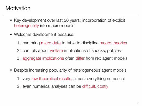
Motivation

• Key development over last 30 years: incorporation of explicitheterogeneity into macro models

• Welcome development because:

1. can bring micro data to table to discipline macro theories2. can talk about welfare implications of shocks, policies3. aggregate implications often differ from rep agent models

• Despite increasing popularity of heterogeneous agent models:

1. very few theoretical results, almost everything numerical2. even numerical analyses can be difficult, costly

2

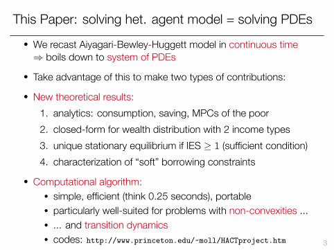
This Paper: solving het. agent model = solving PDEs• We recast Aiyagari-Bewley-Huggett model in continuous time⇒ boils down to system of PDEs

• Take advantage of this to make two types of contributions:

• New theoretical results:1. analytics: consumption, saving, MPCs of the poor2. closed-form for wealth distribution with 2 income types3. unique stationary equilibrium if IES ≥ 1 (sufficient condition)4. characterization of “soft” borrowing constraints

• Computational algorithm:• simple, efficient (think 0.25 seconds), portable• particularly well-suited for problems with non-convexities ...• ... and transition dynamics• codes: http://www.princeton.edu/~moll/HACTproject.htm 3

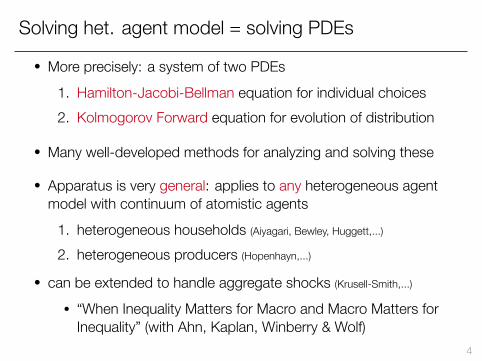
Solving het. agent model = solving PDEs

• More precisely: a system of two PDEs1. Hamilton-Jacobi-Bellman equation for individual choices2. Kolmogorov Forward equation for evolution of distribution

• Many well-developed methods for analyzing and solving these

• Apparatus is very general: applies to any heterogeneous agentmodel with continuum of atomistic agents

1. heterogeneous households (Aiyagari, Bewley, Huggett,...)

2. heterogeneous producers (Hopenhayn,...)

• can be extended to handle aggregate shocks (Krusell-Smith,...)

• “When Inequality Matters for Macro and Macro Matters forInequality” (with Ahn, Kaplan, Winberry & Wolf)

4

Workhorse Model of Income and WealthDistribution in Macroeconomics

5

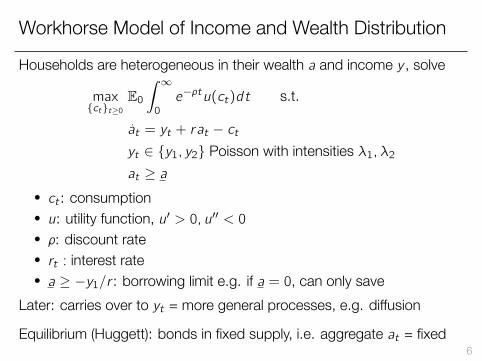
Workhorse Model of Income and Wealth Distribution

Households are heterogeneous in their wealth a and income y , solve

max{ct}t≥0

E0∫ ∞0

e−ρtu(ct)dt s.t.

at = yt + rat − ctyt ∈ {y1, y2} Poisson with intensities λ1, λ2at ≥ a

• ct : consumption• u: utility function, u′ > 0, u′′ < 0• ρ: discount rate• rt : interest rate• a ≥ −y1/r : borrowing limit e.g. if a = 0, can only save

Later: carries over to yt = more general processes, e.g. diffusion

Equilibrium (Huggett): bonds in fixed supply, i.e. aggregate at = fixed6

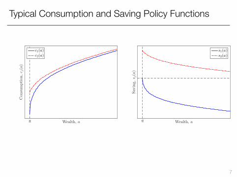
Typical Consumption and Saving Policy Functions

Wealth, a

Con

sumption

,c j(a)

a

c1(a)c2(a)

Wealth, a

Sav

ing,

sj(a)

a

s1(a)s2(a)

7

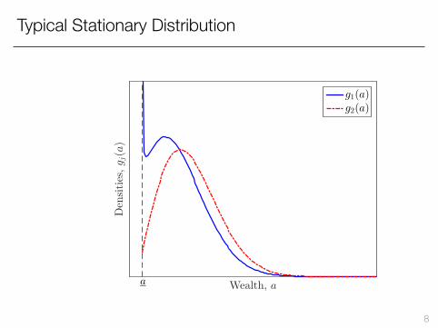
Typical Stationary Distribution

Wealth, a

Den

sities,gj(a)

a

g1(a)g2(a)

8

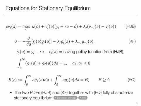
Equations for Stationary Equilibrium

ρvj(a) = maxcu(c) + v ′j (a)(yj + ra − c) + λj(v−j(a)− vj(a)) (HJB)

0 = −d

da[sj(a)gj(a)]− λjgj(a) + λ−jg−j(a), (KF)

sj(a) = yj + ra − cj(a) = saving policy function from (HJB),∫ ∞a

(g1(a) + g2(a))da = 1, g1, g2 ≥ 0

S(r) :=

∫ ∞a

ag1(a)da +

∫ ∞a

ag2(a)da = B, B ≥ 0 (EQ)

• The two PDEs (HJB) and (KF) together with (EQ) fully characterizestationary equilibrium Derivation of (HJB) (KF)

9

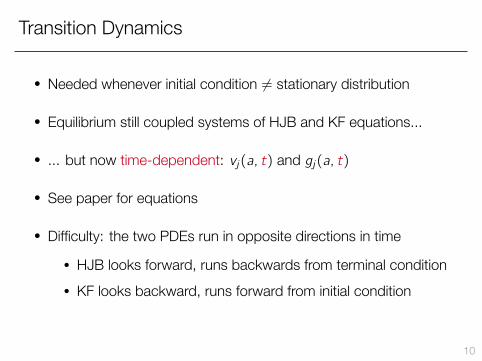
Transition Dynamics

• Needed whenever initial condition = stationary distribution

• Equilibrium still coupled systems of HJB and KF equations...

• ... but now time-dependent: vj(a, t) and gj(a, t)

• See paper for equations

• Difficulty: the two PDEs run in opposite directions in time

• HJB looks forward, runs backwards from terminal condition• KF looks backward, runs forward from initial condition

10

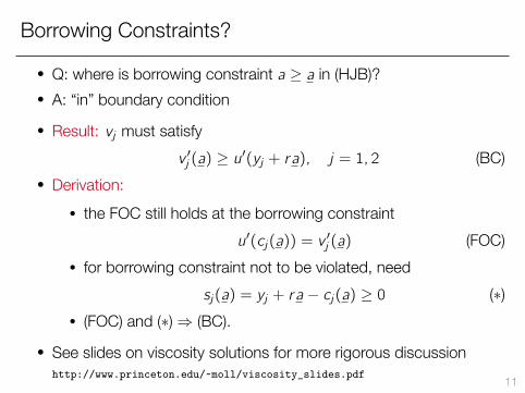
Borrowing Constraints?

• Q: where is borrowing constraint a ≥ a in (HJB)?• A: “in” boundary condition

• Result: vj must satisfyv ′j (a) ≥ u′(yj + ra), j = 1, 2 (BC)

• Derivation:• the FOC still holds at the borrowing constraint

u′(cj(a)) = v′j (a) (FOC)

• for borrowing constraint not to be violated, needsj(a) = yj + ra − cj(a) ≥ 0 (∗)

• (FOC) and (∗)⇒ (BC).

• See slides on viscosity solutions for more rigorous discussionhttp://www.princeton.edu/~moll/viscosity_slides.pdf 11

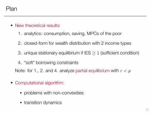
Plan

• New theoretical results:1. analytics: consumption, saving, MPCs of the poor

2. closed-form for wealth distribution with 2 income types

3. unique stationary equilibrium if IES ≥ 1 (sufficient condition)

4. “soft” borrowing constraintsNote: for 1., 2. and 4. analyze partial equilibrium with r < ρ

• Computational algorithm:

• problems with non-convexities

• transition dynamics12

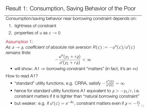
Result 1: Consumption, Saving Behavior of the PoorConsumption/saving behavior near borrowing constraint depends on:

1. tightness of constraint2. properties of u as c → 0

Assumption 1:As a→ a, coefficient of absolute risk aversion R(c) := −u′′(c)/u′(c)remains finite

−u′′(y1 + ra)

u′(y1 + ra)<∞

• will show: A1⇒ borrowing constraint “matters” (in fact, it’s an⇔)How to read A1?

• “standard” utility functions, e.g. CRRA, satisfy −u′′(0)u′(0) =∞

• hence for standard utility functions A1 equivalent to a > −y1/r , i.e.constraint matters if it is tighter than “natural borrowing constraint”

• but weaker: e.g. if u′(c) = e−θc , constraint matters even if a = − y1r 13

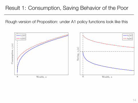
Result 1: Consumption, Saving Behavior of the Poor

Rough version of Proposition: under A1 policy functions look like this

Wealth, a

Con

sumption

,c j(a)

a

c1(a)c2(a)

Wealth, aSav

ing,

sj(a)

a

s1(a)s2(a)

14

Result 1: Consumption, Saving Behavior of the Poor

Proposition: Assume r < ρ, y1 < y2 and that A1 holds.Then saving and consumption policy functions close to a = a satisfy

s1(a) ∼ −√2ν1√a − a

c1(a) ∼ y1 + ra +√2ν1√a − a

c ′1(a) ∼ r +1

2

√ν1

2(a − a)

where ν1 = constant that depends on r, ρ, λ1, λ2 etc – see next slide

Note: “f (a) ∼ g(a)” means lima→a f (a)/g(a) = 1, “f behaves like g close to a”

15

Result 1: Consumption, Saving Behavior of the Poor

Corollary: The wealth of worker who keeps y1 converges to borrowingconstraint in finite time at speed governed by ν1:

a(t)− a ∼ν12(T − t)2 , T := “hitting time” =

√2(a0−a)ν1, 0 ≤ t ≤ T

Proof: integrate a(t) = −√2ν1√a(t)− a

And have analytic solution for speed

ν1 =(ρ− r)u′(c1) + λ1(u′(c1)− u′(c2))

−u′′(c1)≈ (ρ− r)IES(c1)c1 + λ1(c2 − c1)

16

Intuition for Result 1: Two Special Cases

• What’s the role of A1? And why the square root?

• Explain using two special cases with analytic solution

• Both cases: no income uncertainty

17

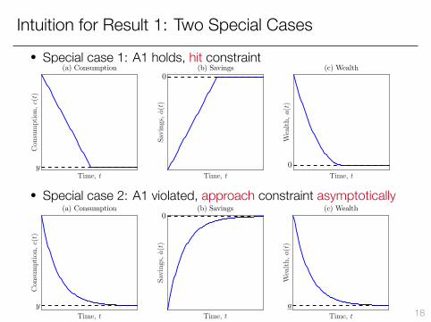
Intuition for Result 1: Two Special Cases• Special case 1: A1 holds, hit constraint

Time, t

Con

sumption

,c(t)

y

(a) Consumption

Time, t

Savings,a(t)

0(b) Savings

Time, t

Wealth,a(t)

0

(c) Wealth

• Special case 2: A1 violated, approach constraint asymptotically

Time, t

Con

sumption

,c(t)

y

(a) Consumption

Time, t

Savings,a(t)

0(b) Savings

Time, t

Wealth,a(t)

a

(c) Wealth

18

Intuition for Result 1: Two Special CasesSpecial case 1: hit constraint

• exponential utility u′(c) = e−θc , tight constraint

c =1

θ(r − ρ), a = y + ra − c, a ≥ 0

• satisfies A1: −u′′(y)u′(y) = θ <∞. Solution:

c(t) = y + ν(T − t), a(t) =ν

2(T − t)2, ν := ρ−r

θ

Special case 2: only approach constraint asymptotically• CRRA utility u′(c) = c−γ , loose constraint

c

c=1

γ(r − ρ), a = y + ra − c, a ≥ a = −

y

r

• violates A1: −u′′(y+ra)u′(y+ra) →∞ as a→ a. Solution:

c(t) = y + (r + η)a(t), a(t)− a = (a0 − a)e−ηt , η := ρ−rγ

19

Intuition for Result 1: Two Special Cases• Special case 1: A1 holds, hit constraint

Time, t

Con

sumption

,c(t)

y

(a) Consumption

Time, t

Savings,a(t)

0(b) Savings

Time, t

Wealth,a(t)

0

(c) Wealth

• Special case 2: A1 violated, approach constraint asymptotically

Time, t

Con

sumption

,c(t)

y

(a) Consumption

Time, t

Savings,a(t)

0(b) Savings

Time, t

Wealth,a(t)

a

(c) Wealth

20

Consumption, Saving Behavior of the Rich

• Skip this today. See paper.

21

Marginal Propensities to Consume and Save

• So far: have characterized c ′j (a) = MPC over discrete time interval• Definition: The MPC over a time period τ is given by

MPCj,τ (a) = C′j,τ (a), where

Cj,τ (a) = E[∫ τ0

cj(at)dt|a0 = a, y0 = yj]

• Lemma: If τ sufficiently small so that no income switches, thenMPC1,τ (a) ∼ min{τc ′1(a), 1 + τr}

Note: MPC1,τ (a) bounded above even though c ′1(a)→∞ as a ↓ a

• If new income draws before τ , no more analytic solution

• But straightforward computation using Feynman-Kacformula22

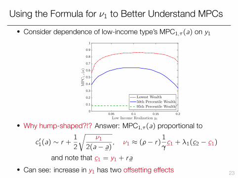
Using the Formula for ν1 to Better Understand MPCs• Consider dependence of low-income type’s MPC1,τ (a) on y1

Low Income Realization y1

0.05 0.1 0.15 0.2

MPC

1,τ(a)

0

0.1

0.2

0.3

0.4

0.5

0.6

0.7

0.8

0.9

1

Lowest Wealth50th Percentile Wealth95th Percentile Wealth

• Why hump-shaped?!? Answer: MPC1,τ (a) proportional to

c ′1(a) ∼ r +1

2

√ν1

2(a − a) , ν1 ≈ (ρ− r)1

γc1 + λ1(c2 − c1)

and note that c1 = y1 + ra• Can see: increase in y1 has two offsetting effects 23

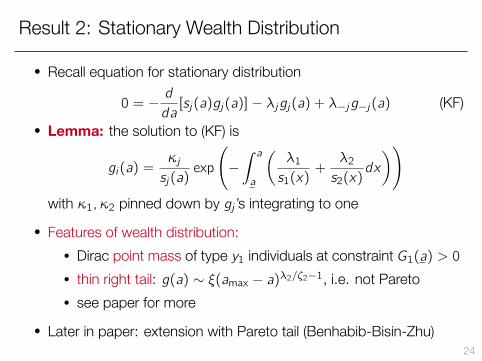
Result 2: Stationary Wealth Distribution

• Recall equation for stationary distribution

0 = −d

da[sj(a)gj(a)]− λjgj(a) + λ−jg−j(a) (KF)

• Lemma: the solution to (KF) is

gi(a) =κjsj(a)

exp

(−∫ aa

(λ1s1(x)

+λ2s2(x)

dx

))with κ1, κ2 pinned down by gj ’s integrating to one

• Features of wealth distribution:• Dirac point mass of type y1 individuals at constraint G1(a) > 0• thin right tail: g(a) ∼ ξ(amax − a)λ2/ζ2−1, i.e. not Pareto• see paper for more

• Later in paper: extension with Pareto tail (Benhabib-Bisin-Zhu)24

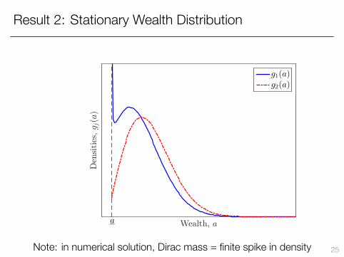
Result 2: Stationary Wealth Distribution

Wealth, a

Den

sities,gj(a)

a

g1(a)g2(a)

Note: in numerical solution, Dirac mass = finite spike in density 25

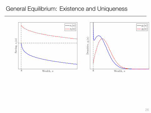
General Equilibrium: Existence and Uniqueness

Wealth, a

Sav

ing,

sj(a)

a

s1(a)s2(a)

Wealth, a

Den

sities,gj(a)

a

g1(a)g2(a)

26

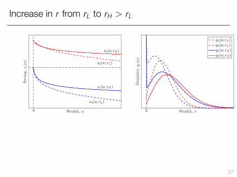
Increase in r from rL to rH > rL

Wealth, a

Sav

ing,

sj(a)

s1(a; rL)

s1(a; rH)

s2(a; rL)

s2(a; rH)

a Wealth, a

Den

sities,gj(a)

a

g1(a; rL)g2(a; rL)g1(a; rH)g2(a; rH)

27

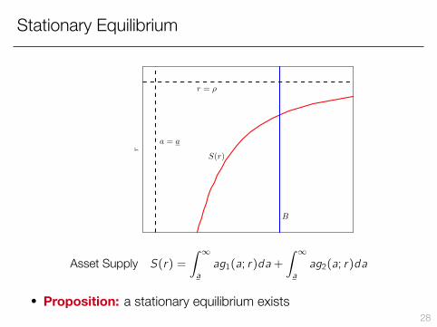
Stationary Equilibrium

r

r = ρ

S(r)

B

a = a

Asset Supply S(r) =

∫ ∞a

ag1(a; r)da +

∫ ∞a

ag2(a; r)da

• Proposition: a stationary equilibrium exists28

Result 3: Uniqueness of Stationary Equilibrium

Proposition: Assume that the IES is weakly greater than one

IES(c) := − u′(c)

u′′(c)c≥ 1 for all c ≥ 0,

and that there is no borrowing a ≥ 0. Then:

1. Individual consumption cj(a; r) is strictly decreasing in r

2. Individual saving sj(a; r) is strictly increasing in r

3. r ↑⇒ CDF Gj(a; r) shifts right in FOSD sense

4. Aggregate saving S(r) is strictly increasing⇒ uniqueness

Note: holds for any labor income process, not just two-state Poisson29

Uniqueness: Proof Sketch

• Parts 2 to 4 direct consequences of part 1 (cj(a; r) decreasing in r )

• ⇒ focus on part 1: builds on nice result by Olivi (2017) whodecomposes ∂cj/∂r into income and substitution effects

• Lemma (Olivi, 2017): c response to change in r is

∂cj(a)

∂r=

1

u′′(c0)E0∫ T0

e−∫ t0 ξsdsu′(ct)dt︸ ︷︷ ︸

substitution effect<0

+1

u′′(c0)E0∫ T0

e−∫ t0 ξsdsu′′(ct)at∂actdt︸ ︷︷ ︸

income effect>0

where ξt := ρ− r + ∂act and T := inf{t ≥ 0|at = 0} = time at which hit 0

• We show: IES(c) := − u′(c)u′′(c)c ≥ 1⇒ substitution effect dominates

⇒ ∂cj(a)/∂r < 0, i.e. consumption decreasing in r

30

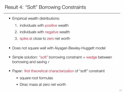
Result 4: “Soft” Borrowing Constraints

• Empirical wealth distributions:

1. individuals with positive wealth2. individuals with negative wealth3. spike at close to zero net worth

• Does not square well with Aiyagari-Bewley-Huggett model

• Simple solution: “soft” borrowing constraint = wedge betweenborrowing and saving r

• Paper: first theoretical characterization of “soft” constraint

• square root formulas• Dirac mass at zero net worth

31

Computations forHeterogeneous Agent Model

32

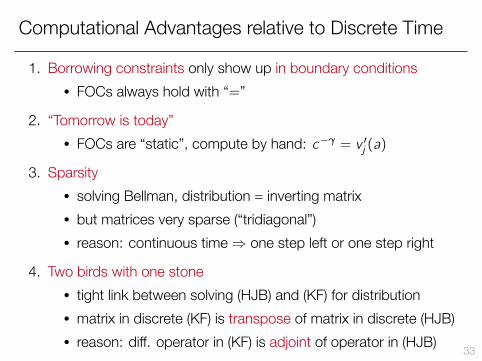
Computational Advantages relative to Discrete Time

1. Borrowing constraints only show up in boundary conditions• FOCs always hold with “=”

2. “Tomorrow is today”• FOCs are “static”, compute by hand: c−γ = v ′j (a)

3. Sparsity• solving Bellman, distribution = inverting matrix• but matrices very sparse (“tridiagonal”)• reason: continuous time⇒ one step left or one step right

4. Two birds with one stone• tight link between solving (HJB) and (KF) for distribution• matrix in discrete (KF) is transpose of matrix in discrete (HJB)• reason: diff. operator in (KF) is adjoint of operator in (HJB) 33

Computations for Heterogeneous Agent Model

• Hard part: HJB equation

• Easy part: KF equation. Once you solved HJB equation, get KFequation “for free”

• System to be solvedρv1(a) = max

cu(c) + v ′1(a)(y1 + ra − c) + λ1(v2(a)− v1(a))

ρv2(a) = maxcu(c) + v ′2(a)(y2 + ra − c) + λ2(v1(a)− v2(a))

0 = −d

da[s1(a)g1(a)]− λ1g1(a) + λ2g2(a)

0 = −d

da[s2(a)g2(a)]− λ2g2(a) + λ1g1(a)

1 =

∫ ∞a

g1(a)da +

∫ ∞a

g2(a)da

B =

∫ ∞a

ag1(a)da +

∫ ∞a

ag2(a)da := S(r)

34

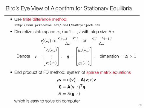
Bird’s Eye View of Algorithm for Stationary Equilibria• Use finite difference method:

http://www.princeton.edu/~moll/HACTproject.htm

• Discretize state space ai , i = 1, ..., I with step size ∆a

v ′j (ai) ≈vi+1,j − vi ,j∆a

or vi ,j − vi−1,j∆a

Denote v =

v1(a1)...v2(aI)

, g =g1(a1)...g2(aI)

, dimension = 2I × 1

• End product of FD method: system of sparse matrix equationsρv = u(v) + A(v; r)v

0 = A(v; r)Tg

B = S(g; r)

which is easy to solve on computer35

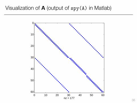
Visualization of A (output of spy(A) in Matlab)

0 10 20 30 40 50 60

0

10

20

30

40

50

60

nz = 177 36

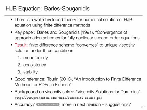
HJB Equation: Barles-Souganidis• There is a well-developed theory for numerical solution of HJB

equation using finite difference methods• Key paper: Barles and Souganidis (1991), “Convergence of

approximation schemes for fully nonlinear second order equations• Result: finite difference scheme “converges” to unique viscosity

solution under three conditions1. monotonicity2. consistency3. stability

• Good reference: Tourin (2013), “An Introduction to Finite DifferenceMethods for PDEs in Finance”

• Background on viscosity soln’s: “Viscosity Solutions for Dummies”http://www.princeton.edu/~moll/viscosity_slides.pdf

• Accuracy? Two experiments , more in next revision – suggestions? 37

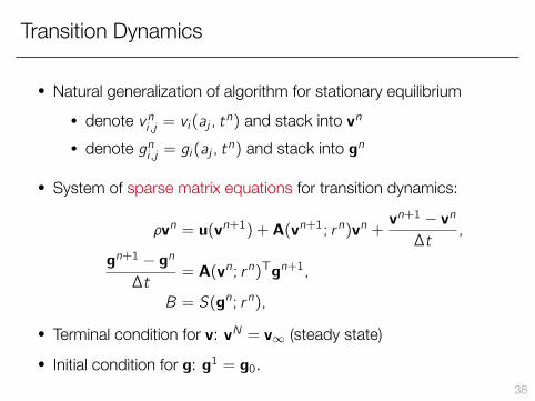
Transition Dynamics

• Natural generalization of algorithm for stationary equilibrium• denote vni,j = vi(aj , tn) and stack into vn

• denote gni,j = gi(aj , tn) and stack into gn

• System of sparse matrix equations for transition dynamics:

ρvn = u(vn+1) + A(vn+1; rn)vn +vn+1 − vn

∆t,

gn+1 − gn

∆t= A(vn; rn)Tgn+1,

B = S(gn; rn),

• Terminal condition for v: vN = v∞ (steady state)

• Initial condition for g: g1 = g0.38

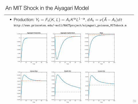
An MIT Shock in the Aiyagari Model

• Production: Yt = Ft(K,L) = AtKαL1−α, dAt = ν(A− At)dthttp://www.princeton.edu/~moll/HACTproject/aiyagari_poisson_MITshock.m

Year0 20 40 60 80 100

0.097

0.0975

0.098

0.0985

0.099

0.0995

0.1

0.1005Aggregate Productivity

Year0 20 40 60 80 100

0.293

0.294

0.295

0.296

0.297

0.298

0.299

0.3Aggregate Capital Stock

Year0 20 40 60 80 100

0.0376

0.0378

0.038

0.0382

0.0384

0.0386

0.0388

0.039Wage

Year0 20 40 60 80 100

0.0445

0.045

0.0455

0.046

0.0465

0.047

0.0475

0.048

0.0485

0.049Interest Rate

Year0 20 40 60 80 100

0.882

0.884

0.886

0.888

0.89

0.892

0.894

0.896Wealth Gini

Year0 20 40 60 80 100

0.236

0.237

0.238

0.239

0.24

0.241

0.242Income Gini

39

Generalizations andOther Applications

40

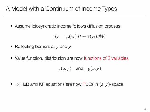
A Model with a Continuum of Income Types

• Assume idiosyncratic income follows diffusion process

dyt = µ(yt)dt + σ(yt)dWt

• Reflecting barriers at y and y

• Value function, distribution are now functions of 2 variables:

v(a, y) and g(a, y)

• ⇒ HJB and KF equations are now PDEs in (a, y)-space

41

It doesn’t matter whether you solve ODEs or PDEs⇒ everything generalizes

http://www.princeton.edu/~moll/HACTproject/huggett_diffusion_partialeq.m

42

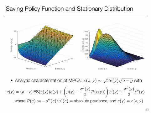
Saving Policy Function and Stationary Distribution

Income, yWealth, a

0.5

0

-0.5

Sav

ings

s(a,y)

Income, yWealth, a

0.15

0.2

0.25

0.3

0.35

0.1

0.05

0

Den

sity

g(a,y)

• Analytic characterization of MPCs: c(a, y) ∼√2ν(y)

√a − a with

ν(y) = (ρ− r)IES(c(y))c(y) +(µ(y)−

σ2(y)

2P(c(y))

)c ′(y) +

σ2(y)

2c ′′(y)

where P(c) := −u′′′(c)/u′′(c) = absolute prudence, and c(y) = c(a, y)

43

Other Applications – see Paper

• Non-convexities: indivisible housing, mortgages, poverty traps

• Fat-tailed wealth distribution

• Multiple assets with adjustment costs (Kaplan-Moll-Violante)

• Stopping time problems

44

Conclusion

• Very general apparatus: solving het. agent model = solving PDEs

• New theoretical results:1. analytics: consumption, saving, MPCs of the poor2. closed-form for wealth distribution with 2 income types3. unique stationary equilibrium if IES ≥ 14. characterization of “soft” borrowing constraints

• Computational algorithm:• simple, efficient, portable• codes: http://www.princeton.edu/~moll/HACTproject.htm

• Large number of potential applications – come talk to me!45

Appendix

46

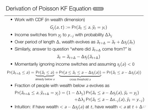
Derivation of Poisson KF Equation Back

• Work with CDF (in wealth dimension)Gj(a, t) := Pr(at ≤ a, yt = yi)

• Income switches from yj to y−j with probability ∆λj• Over period of length ∆, wealth evolves as at+∆ = at + ∆sj(at)• Similarly, answer to question “where did at+∆ come from?” is

at = at+∆ − ∆sj(at+∆)• Momentarily ignoring income switches and assuming sj(a) < 0Pr(at+∆ ≤ a) = Pr(at ≤ a)︸ ︷︷ ︸

already below a

+Pr(a ≤ at ≤ a − ∆sj(a))︸ ︷︷ ︸cross threshold a

= Pr(at ≤ a − ∆sj(a))

• Fraction of people with wealth below a evolves asPr(at+∆ ≤ a, yt+∆ = yj) = (1− ∆λj) Pr(at ≤ a − ∆sj(a), yt = yj)

+∆λj Pr(at ≤ a − ∆s−j(a), yt = y−j)• Intuition: if have wealth < a− ∆sj(a) at t, have wealth < a at t +∆47

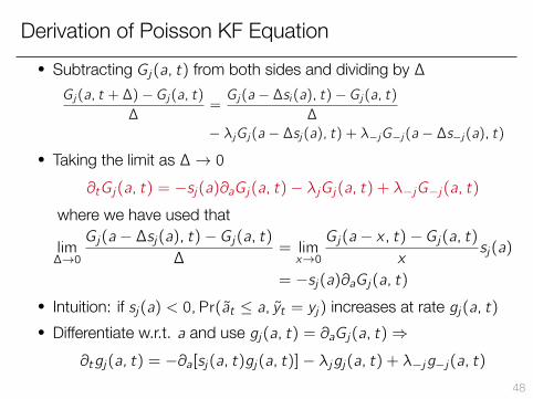
Derivation of Poisson KF Equation• Subtracting Gj(a, t) from both sides and dividing by ∆Gj(a, t + ∆)− Gj(a, t)

∆=Gj(a − ∆si(a), t)− Gj(a, t)

∆

− λjGj(a − ∆sj(a), t) + λ−jG−j(a − ∆s−j(a), t)

• Taking the limit as ∆→ 0∂tGj(a, t) = −sj(a)∂aGj(a, t)− λjGj(a, t) + λ−jG−j(a, t)

where we have used that

lim∆→0

Gj(a − ∆sj(a), t)− Gj(a, t)∆

= limx→0

Gj(a − x, t)− Gj(a, t)x

sj(a)

= −sj(a)∂aGj(a, t)• Intuition: if sj(a) < 0,Pr(at ≤ a, yt = yj) increases at rate gj(a, t)• Differentiate w.r.t. a and use gj(a, t) = ∂aGj(a, t)⇒

∂tgj(a, t) = −∂a[sj(a, t)gj(a, t)]− λjgj(a, t) + λ−jg−j(a, t)48

Accuracy of Finite Difference Method?

Two experiments:

1. special case: comparison with closed-form solution

2. general case: comparison with numerical solution computed usingvery fine grid

49

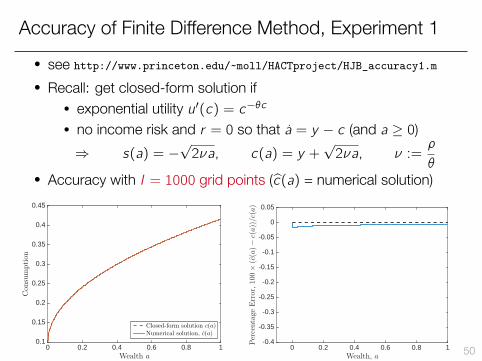
Accuracy of Finite Difference Method, Experiment 1• see http://www.princeton.edu/~moll/HACTproject/HJB_accuracy1.m

• Recall: get closed-form solution if• exponential utility u′(c) = c−θc• no income risk and r = 0 so that a = y − c (and a ≥ 0)⇒ s(a) = −

√2νa, c(a) = y +

√2νa, ν :=

ρ

θ• Accuracy with I = 1000 grid points (c(a) = numerical solution)

Wealth a

0 0.2 0.4 0.6 0.8 1

Con

sumption

0.1

0.15

0.2

0.25

0.3

0.35

0.4

0.45

Closed-form solution c(a)Numerical solution, c(a)

Wealth, a0 0.2 0.4 0.6 0.8 1

Percentage

Error,100×(c(a)−c(a))/c(a)

-0.4

-0.35

-0.3

-0.25

-0.2

-0.15

-0.1

-0.05

0

0.05

50

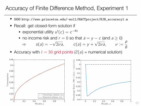
Accuracy of Finite Difference Method, Experiment 1• see http://www.princeton.edu/~moll/HACTproject/HJB_accuracy1.m

• Recall: get closed-form solution if• exponential utility u′(c) = c−θc• no income risk and r = 0 so that a = y − c (and a ≥ 0)⇒ s(a) = −

√2νa, c(a) = y +

√2νa, ν :=

ρ

θ• Accuracy with I = 30 grid points (c(a) = numerical solution)

Wealth a

0 0.2 0.4 0.6 0.8 1

Con

sumption

0.1

0.15

0.2

0.25

0.3

0.35

0.4

0.45

Closed-form solution c(a)Numerical solution, c(a)

Wealth, a0 0.2 0.4 0.6 0.8 1

Percentage

Error,100×(c(a)−c(a))/c(a)

-0.4

-0.35

-0.3

-0.25

-0.2

-0.15

-0.1

-0.05

0

0.05

51

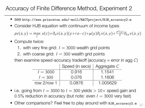
Accuracy of Finite Difference Method, Experiment 2• see http://www.princeton.edu/~moll/HACTproject/HJB_accuracy2.m

• Consider HJB equation with continuum of income typesρv(a, y) = max

cu(c)+∂av(a, y)(y+ra−c)+µ(y)∂yv(a, y)+σ

2(y)2 ∂yyv(a, y)

• Compute twice:1. with very fine grid: I = 3000 wealth grid points2. with coarse grid: I = 300 wealth grid points

then examine speed-accuracy tradeoff (accuracy = error in agg C)Speed (in secs) Aggregate C

I = 3000 0.916 1.1541I = 300 0.076 1.1606

row 2/row 1 0.0876 1.005629• i.e. going from I = 3000 to I = 300 yields > 10× speed gain and0.5% reduction in accuracy (but note: even I = 3000 very fast)

• Other comparisons? Feel free to play around with HJB_accuracy2.m 52