Income and Wealth Heterogeneity in the Macroeconomy · Anthony A. Smith, Jr. ... We characterize stationary stochastic equilibria of this model nu-merically, and we then compare the

Income and Wealth Heterogeneity in theMacroeconomy

Per KrusellUniversity of Rochester, Centre for Economic Policy Research, and Institute forInternational Economic Studies

Anthony A. Smith, Jr.Carnegie Mellon University

How do movements in the distribution of income and wealth affectthe macroeconomy? We analyze this question using a calibratedversion of the stochastic growth model with partially uninsurableidiosyncratic risk and movements in aggregate productivity. Ourmain finding is that, in the stationary stochastic equilibrium, thebehavior of the macroeconomic aggregates can be almost perfectlydescribed using only the mean of the wealth distribution. This re-sult is robust to substantial changes in both parameter values andmodel specification. Our benchmark model, whose only differencefrom the representative-agent framework is the existence of unin-surable idiosyncratic risk, displays far less cross-sectional dispersion

We thank conference participants at Macroeconomics with ‘‘Frictions,’’ held atthe Federal Reserve Bank of Minneapolis; the National Bureau of Economic Re-search Summer Workshop on the Aggregate Implications of Microeconomic Con-sumption Behavior; the Northwestern Summer Workshop on Applied General Equi-librium Analysis; the annual meetings of the Society for Economic Dynamics andControl; the North American summer meetings of the Econometric Society; andthe Stanford Institute for Theoretical Economics Summer Workshop and seminarparticipants at Carnegie Mellon, Columbia, Institute for International EconomicStudies, Pompeu Fabra, Southern Methodist University, Texas at Austin, Wharton,Yale, and York. We also benefited particularly from comments by Wouter den Haan,Mark Huggett, Robert Lucas, Vıctor Rıos-Rull, Tom Sargent, Jose Scheinkman, ChrisTelmer, Stan Zin, and two anonymous referees. Financial support from the Bank ofSweden Tercentenary Foundation, the National Science Foundation, and the SocialSciences and Humanities Research Council of Canada is gratefully acknowledged.

[Journal of Political Economy, 1998, vol. 106, no. 5] 1998 by The University of Chicago. All rights reserved. 0022-3808/98/0605-0003$02.50

867

868 journal of political economyand skewness in wealth than U.S. data. However, an extension thatrelies on a small amount of heterogeneity in thrift does succeedin replicating the key features of the wealth data. Furthermore,this extension features aggregate time series that depart signifi-cantly from permanent income behavior.

I. Introduction

Most of dynamic general equilibrium macroeconomic theory reliesheavily on the representative-agent abstraction: it is assumed thatthe economy behaves ‘‘as if ’’ it is inhabited by a single (type of)consumer. At the same time, this macroeconomic theorizing at-tempts to take microfoundations seriously; the parameters of themodels are typically selected on the basis of existing empirical andtheoretical knowledge, and the models are then used to generatequantitative statements. At first glance, the representative-agent as-sumption appears to be inconsistent with a serious treatment of mi-crofoundations. There are two circumstances, however, under whichthe representative-agent construct would be a reasonable modelingstrategy. First, it is possible that the theoretical assumptions neededto justify the use of a representative consumer are roughly met inthe data. This view, however, is hard to defend; one problem is thatit is difficult to justify the assumption that there are complete insur-ance markets for consumers’ idiosyncratic risks. A second possibilityis that the aggregate variables in theoretical models with a more real-istic description of the microeconomic environment actually behavelike those in the representative-agent models. In this paper we beginthe exploration of this second possibility.

The goal of the present analysis is to extend the standard macro-economic model to include substantial heterogeneity in income andwealth. More precisely, we consider a calibrated version of the sto-chastic growth model in which there is a large number of consumerswho, in addition to uncertain aggregate productivity, face idiosyn-cratic income (employment) shocks. Following Bewley (1977),Scheinkman and Weiss (1986), and others, we assume that consum-ers cannot insure directly against these shocks, but that they can buyand sell an asset subject to an exogenous lower bound on the assetholding. In our macroeconomic framework, as in Aiyagari (1994),this asset is aggregate capital. Savings can thus be precautionary andallow partial insurance against the idiosyncratic shocks. Because ofthe lack of full insurance, this model generates an endogenous distri-bution of wealth across consumers. An important problem, there-fore, is how to characterize the interaction between the distributionof wealth and the macroeconomic aggregates.

income and wealth heterogeneity 869

We characterize stationary stochastic equilibria of this model nu-merically, and we then compare the aggregate properties of theseequilibria with those implied by the corresponding representative-agent model. The characterization of the stochastic behavior of theincome and wealth distributions is central to our task since aggregatevariables depend on these distributions. An important componentof our analysis involves dealing with the main computational diffi-culty of dynamic heterogeneous-agent models: in order to predictprices, consumers need to keep track of the evolution of the wealthdistribution. One of the contributions of our work is to show howequilibria can be approximated numerically, despite the fact thatthe state of the economy at any point in time is an infinite-dimen-sional object (we assume a continuum of agents). This methodologi-cal contribution opens the possibility of characterizing a large classof new macroeconomic models in which heterogeneity in incomeand wealth plays a key role. For example, this class of models allowsa much richer analysis of the interactions between business cyclesand inequality than existing frameworks do.

Our main insight is that the macroeconomic model with heteroge-neity features approximate aggregation. By approximate aggregation,we mean that, in equilibrium, all aggregate variables—consumption,the capital stock, and relative prices—can be almost perfectly de-scribed as a function of two simple statistics: the mean of the wealthdistribution and the aggregate productivity shock. Therefore, theconsumers in our equilibrium face manageable prediction problemssince the distribution of aggregate wealth is almost completely irrele-vant for how the aggregates behave in the equilibrium. Furthermore,this finding is remarkably robust to changes in both parameter val-ues and the specification of the model.

When the representative-agent model is altered only by addingidiosyncratic, uninsurable risk, the resulting stationary wealth distri-bution is quite unrealistic: there are too few very poor agents, andmuch too little concentration of wealth among the very richest. Forthis reason, we consider a version of the model with preference het-erogeneity: agents have random discount factors, whose values havea symmetric distribution with a small variance and whose transitionprobabilities are such that the average duration, or life length, of adiscount factor equals that of a generation. In this fashion, we incor-porate genetic differences in the population that are passed on im-perfectly from parents to children. We show that this model doessucceed quite well in matching the key features of the wealth distri-bution.

The model with preference heterogeneity also gives rise to inter-esting aggregate time-series behavior. In this model, although aggre-

870 journal of political economy

gate wealth is mainly in the hands of the rich, poor agents have alarge influence on aggregate consumption. Since these agents arealso impatient on average, they can be characterized as ‘‘hand-to-mouth’’ consumers. Thus, in the aggregate, we observe a significantdeparture from permanent income behavior, in contrast to standardrepresentative-agent models.

The explanation for our main result—the collapse of the statespace—builds on the properties of optimal savings behavior in ourclass of models. The key insight is related to earlier findings fromsimilar models that utility costs from fluctuations in consumptionare quite small and that self-insurance with only one asset is quiteeffective.1 Self-insurance in our model is not very effective in termsof smoothing individual relative to aggregate consumption; for ex-ample, the unconditional standard deviation of individual consump-tion is about four times that of aggregate consumption, and the un-conditional correlation of the consumption of any two agents is veryclose to zero. However, in utility terms, agents in our stationary equi-libria are insured well enough that the marginal propensity to saveout of current wealth is almost completely independent of the levelsof wealth and labor income, except at the very lowest levels of wealth.Furthermore, although some very poor agents have substantially dif-ferent marginal savings propensities at any point in time, the frac-tion of total wealth held by these agents is always very small (this isparticularly true in the model with a realistic wealth distribution).Because it is so small, higher-order moments of the wealth distribu-tion simply do not affect the accumulation pattern of total capital,even though these moments do move significantly over time.

Our computational algorithm is essential for understanding howour approximate equilibrium differs from an exact equilibrium. Themain computational task is to calculate the law of motion for thedistribution of capital over individuals. Our approach is to calculateequilibria in which, by assumption, agents have a limited ability topredict the evolution of this distribution. We then show that thisbound on ability almost does not constrain the agents at all. Moreprecisely, we compute approximate equilibria by postulating that thelaw of motion perceived by agents can be described by a stochasticprocess for a finite-dimensional vector of moments of the wealthdistribution. For any given vector of moments m, a candidate ap-proximate equilibrium is a fixed point in a class 6 of (possibly non-

1 See, e.g., Robert Lucas (1987), Cochrane (1989), and Krusell and Smith (1996b)and the incomplete-markets asset pricing literature as represented by Marcet andSingleton (1991), Telmer (1993), Deborah Lucas (1994), Heaton and Lucas (1995,1996), den Haan (1996a, 1996b), and Krusell and Smith (1997).


linear) first-order Markov processes. A given Markov process S ∈ 6is a fixed point if (1) agents’ decision rules derive from dynamicmaximization problems in which the behavior of the aggregate stateis described by S and (2) S is the best approximation in the class 6to the dynamic behavior of m implied by the aggregated decisionrules of agents. In other words, the calculated object satisfies all thestandard equilibrium conditions except the agents’ ability to makeperfect forecasts. One way to assess how much this ability is con-strained is to measure how well individual agents can forecast futureprices using S. We use a measure of forecasting accuracy in the algo-rithm to decide whether to increase the agents’ ability to make fore-casts—increase the dimension of m or expand the class 6—or tostop. In these terms, our main finding is that, when 6 is the class oflinear first-order Markov processes and m consists only of the meanof the distribution of capital, we obtain extremely high forecastingaccuracy. The accuracy is so high that we find it very hard to argueon the basis of the ‘‘irrationality’’ of the agents in our model thatour approximate equilibrium is a less satisfactory economic modelthan an exact equilibrium.

In Sections II and III we describe the benchmark model, the com-putational strategy, and the main result. Section IV discusses thewealth distribution data and presents the model with preference het-erogeneity. That section also describes the aggregate time-series sta-tistics from the various models and makes comparisons with repre-sentative-agent models. Section V concludes with some remarks.

II. Model Framework

In this section we describe our model economy. The key source ofheterogeneity is an assumption that idiosyncratic income shocks arepartially uninsurable. In our benchmark setup there is only one typeof consumer (i.e., all consumers have the same preferences), andthe setup is one that in all other ways is like the standard stochasticgrowth model. Later, in Section IV, we extend the benchmark modelto include preference heterogeneity.

A. The Environment

We consider a version of the stochastic growth model with a large(measure one) population of infinitely lived consumers. There isonly one good per period, and we assume that the preferences overstreams of consumption of each agent are given by


E 0 ^∞

t50

βt U(ct ),

with

U(c) 5 limν →σ

c 12ν 2 11 2 ν

.

Production of the good, y, is a Cobb-Douglas function of capitalinput, k, and labor input l : y 5 zkαl 12α, with α ∈ [0, 1]. The outputcan be transformed into future capital, k ′, and current consumptionaccording to

c 1 k ′ 2 (1 2 δ)k 5 y,

where δ ∈ [0, 1] is the rate of depreciation.Each agent is endowed with one unit of time, which gives rise to

e l units of labor input, where e is stochastic and can take on thevalue zero or one. When e 5 1, we think of the agent as employedand supplying l units of labor input; when e 5 0, we think of himas unemployed. There is also a stochastic shock to aggregate produc-tivity, which we denote z. There are two possible aggregate states:either the state is good, and z 5 z g, or it is bad, and z 5 z b. Theaggregate shock follows a first-order Markov structure given by thetransition probabilities πss ′: the probability that the aggregate shocknext period is z s ′ given that it is z s this period. The individual andaggregate shocks are correlated, and the individuals’ shocks are as-sumed to satisfy a law of large numbers. By virtue of the law of largenumbers, the only exogenous source of aggregate uncertainty in theeconomy is the aggregate productivity shock. More specifically, thenumber of agents who are unemployed always equals ug in goodtimes and ub in bad times. In other words, when one controls forz, individual shocks are uncorrelated. We use πss ′ee′ to denote theprobability of transition from state (z s, e) today to (z s ′, e′) tomorrow.The transition probabilities have to satisfy the restrictions

πss ′00 1 πss ′01 5 πss ′10 1 πss ′11 5 πss ′

and

usπss ′00

πss ′1 (1 2 u s)

πss ′10

πss ′5 us ′

for all four possible values of (s, s ′).


B. The Market Arrangement

For the economic environment described above, the assumption ofcomplete markets gives an aggregation theorem: it is possible to de-termine full contingent plans for total capital accumulation and tosolve for all state-contingent prices without knowing how wealth isdistributed across consumers.2 Here, however, we assume that thereare incomplete markets: there is only one asset—capital. This assetplays the twin roles of being a store of value for the individual agentand a means of self-insurance against the income shocks.3 Thus letk denote the holdings of capital. In order to rule out Ponzi schemesand to guarantee that loans are paid back, we restrict capital hold-ings to satisfy k ∈_ ; [0, ∞).4 We refer to the lower bound on capitalas the borrowing constraint.

Consumers collect income from working and from the services oftheir capital. If the total amount of capital in the economy is denotedk and the total amount of labor supplied is denoted l , our constant-returns-to-scale production function implies that the relevant pricesare w(k, l , z) 5 (1 2 α)z(k/l )α and r(k, l , z) 5 αz(k/l )α21, re-spectively.

We consider a recursive equilibrium definition, which includes,then, as a key element, a law of motion of the aggregate state of theeconomy. The aggregate state is (Γ, z), where Γ denotes the currentmeasure (distribution) of consumers over holdings of capital andemployment status. The part of the law of motion that concernsz is exogenous; it can be described by z ’s transition matrix. Thepart that concerns updating Γ is denoted H ; in other words, Γ′ 5H(Γ, z, z ′). For the individual agent, the relevant state variable is hisholdings of capital, his employment status, and the aggregate state:(k, e; Γ, z). The role of the aggregate state is to allow the consumerto predict future prices. His optimization problem can therefore beexpressed as

v(k, e; Γ, z) 5 maxc ,k ′

{U(c) 1 βE[v(k ′, e′; Γ′, z ′) |z, e]}

2 See Chatterjee (1994) or Krusell and Rıos-Rull (1997) for a discussion.3 In this respect, our approach parallels those adopted in a number of recent

papers, including Imrohoroglu (1989, 1992), Aiyagari and Gertler (1991), Dıaz-Gimenez et al. (1992), Huggett (1993), and Aiyagari (1994).

4 One could also consider a negative lower bound on holdings of capital. As Aiya-gari (1994) shows in a model without aggregate productivity shocks, if the lowestindividual income realization is zero, then a constraint to always pay back impliesthat a lower bound for capital that is less than zero is equivalent to one that is zero.In this sense, our lower bound is generous. Later, we also consider positive lowerbounds.


subject to

c 1 k ′ 5 r(k, l , z)k 1 w(k, l , z) le 1 (1 2 δ)k,

Γ′ 5 H(Γ, z, z ′),

k ′ $ 0

and the stochastic laws of motion for z and e. The decision rule forthe updating of capital implied by this problem is denoted by thefunction f : k ′ 5 f(k, e; Γ, z).

A recursive competitive equilibrium is then a law of motion H, apair of individual functions v and f, and pricing functions (r, w)such that (i) (v, f ) solves the consumer’s problem, (ii) r and w arecompetitive (i.e., given by marginal productivities as expressedabove), and (iii) H is generated by f, that is, the appropriate sum-ming up of agents’ optimal choices of capital given their currentstatus in terms of wealth and employment.

C. Computational Strategy

We now outline our algorithm for computing equilibria numeri-cally.5 This description is nontechnical and is included in the mainbody of the paper because the procedures are intimately connectedwith the economic mechanisms we wish to emphasize. The endoge-nous state variable of the economy, Γ, is a high-dimensional object.It is well known that numerical solution of dynamic programmingproblems becomes increasingly difficult as the size of the state spaceincreases. Our way of dealing with this problem is to assume thatagents are boundedly rational in their perceptions of how Γ evolvesover time and to increase the sophistication of these perceptionsuntil the errors that agents make because they are not fully rationalbecome negligible.

Therefore, suppose that agents do not perceive current or futureprices as depending on anything more than the first I moments ofΓ (in addition to z); denote these moments as m ; (m1, m2, . . . ,m I).6 Since current prices depend only on the total amount of capi-tal and not on its distribution, limiting agents to a finite set of mo-ments is restrictive only as far as future prices are concerned. Inparticular, to know future prices, it is necessary to know how thetotal capital stock evolves. Since savings decisions do not aggregate,

5 Our algorithm bears some similarities to one proposed in Dıaz-Gimenez andRıos-Rull (1991).

6 By m1 we are referring to a 2 3 1 vector consisting of the first moments of Γ;m2 is a 2 3 2 matrix consisting of the second moments of Γ, and so on.


the total capital stock in the future is a nontrivial function of all themoments of the current distribution.

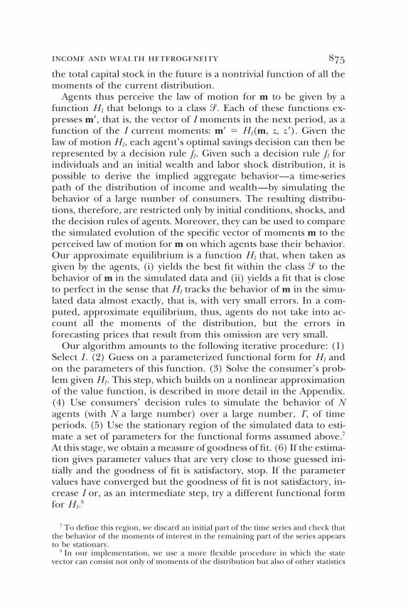
Agents thus perceive the law of motion for m to be given by afunction HI that belongs to a class 6. Each of these functions ex-presses m′, that is, the vector of I moments in the next period, as afunction of the I current moments: m′ 5 HI(m, z, z ′). Given thelaw of motion HI, each agent’s optimal savings decision can then berepresented by a decision rule fI. Given such a decision rule fI forindividuals and an initial wealth and labor shock distribution, it ispossible to derive the implied aggregate behavior—a time-seriespath of the distribution of income and wealth—by simulating thebehavior of a large number of consumers. The resulting distribu-tions, therefore, are restricted only by initial conditions, shocks, andthe decision rules of agents. Moreover, they can be used to comparethe simulated evolution of the specific vector of moments m to theperceived law of motion for m on which agents base their behavior.Our approximate equilibrium is a function HI that, when taken asgiven by the agents, (i) yields the best fit within the class 6 to thebehavior of m in the simulated data and (ii) yields a fit that is closeto perfect in the sense that HI tracks the behavior of m in the simu-lated data almost exactly, that is, with very small errors. In a com-puted, approximate equilibrium, thus, agents do not take into ac-count all the moments of the distribution, but the errors inforecasting prices that result from this omission are very small.

Our algorithm amounts to the following iterative procedure: (1)Select I . (2) Guess on a parameterized functional form for HI andon the parameters of this function. (3) Solve the consumer’s prob-lem given HI. This step, which builds on a nonlinear approximationof the value function, is described in more detail in the Appendix.(4) Use consumers’ decision rules to simulate the behavior of Nagents (with N a large number) over a large number, T, of timeperiods. (5) Use the stationary region of the simulated data to esti-mate a set of parameters for the functional forms assumed above.7

At this stage, we obtain a measure of goodness of fit. (6) If the estima-tion gives parameter values that are very close to those guessed ini-tially and the goodness of fit is satisfactory, stop. If the parametervalues have converged but the goodness of fit is not satisfactory, in-crease I or, as an intermediate step, try a different functional formfor HI.8

7 To define this region, we discard an initial part of the time series and check thatthe behavior of the moments of interest in the remaining part of the series appearsto be stationary.

8 In our implementation, we use a more flexible procedure in which the statevector can consist not only of moments of the distribution but also of other statistics


As an illustration, consider the following example. Assume thatI 5 1 and that HI is log-linear:

z 5 z g : log k ′ 5 a 0 1 a 1 log k,

z 5 z b : log k ′ 5 b 0 1 b 1 log k.

The agent then solves the following problem:

v(k, e; k, z) 5 maxc ,k ′

{U(c) 1 βE[v(k ′, e′; k ′, z ′) |z, e]}

subject to

c 1 k ′ 5 r(k, l , z)k 1 w(k, l , z)le 1 (1 2 δ)k,

log k ′ 5 a 0 1 a 1 log k if z 5 z g,

log k ′ 5 b 0 1 b 1 log k if z 5 z b ,

k ′ $ 0

and the law of motion for (z, e). We thus obtain a (nonlinear) deci-sion rule k ′ 5 fI(k, e; k, z) that, when simulated, allows us to comparethe aggregate behavior of the moments with their description HI.The idea is thus to find a fixed point for HI in the form of a vector(a*0 , a*1 , b*0 , b*1 ). If this HI is satisfactorily reproduced in simulations(i.e., if the goodness of fit is high), stop. Otherwise, consider a moreflexible functional form for HI or add another moment.

III. Results

We shall now show our approximate aggregation result for thebenchmark model. Our approach is to select parameter values thatare in line with those used in similar studies (which in turn are basedon microeconomic data or long-run model considerations) andthen to examine whether the results are robust to changes in theparameter values. We comment on the robustness analysis at the endof this section.

A. Model Parameters for the Benchmark Setup

We use β 5 0.99 and δ 5 0.025, reflecting a period of one quarter,a relative risk aversion parameter σ of 1, and a capital share α of0.36. We set the shock values to z g 5 1.01 and z b 5 0.99 and theunemployment rates to ug 5 0.04 and ub 5 0.1, implying that the

describing the distribution, such as tail probabilities, which are themselves nonlinearfunctions of the distribution’s moments.


fluctuations in the macroeconomic aggregates have roughly thesame magnitude as the fluctuations in observed postwar U.S. timeseries. The process for (z, e) is chosen so that the average durationof both good and bad times is eight quarters and so that the aver-age duration of an unemployment spell is 1.5 quarters in goodtimes and 2.5 quarters in bad times. We also impose πgb00π21

gb 51.25πbb00π21

bb and πbg00π21bg 5 0.75πgg00π21

gg .9

B. Solution and Simulation Parameters

We solve the consumer’s problem by computing an approximationto the value function on a grid of points in the state space. We usecubic spline and polynomial interpolation to compute the valuefunction at points not on the grid. See the Appendix for a detaileddescription of the numerical algorithm used to solve the consumer’sproblem. In our simulations we include 5,000 agents and 11,000 pe-riods; we discard the first 1,000 time periods. Typically, the initialwealth distribution in the simulations is one in which all agents holdthe same level of assets. We find that our results are not sensitive tochanges in the initial wealth distribution.

C. Equilibrium Properties: Only the Mean Matters

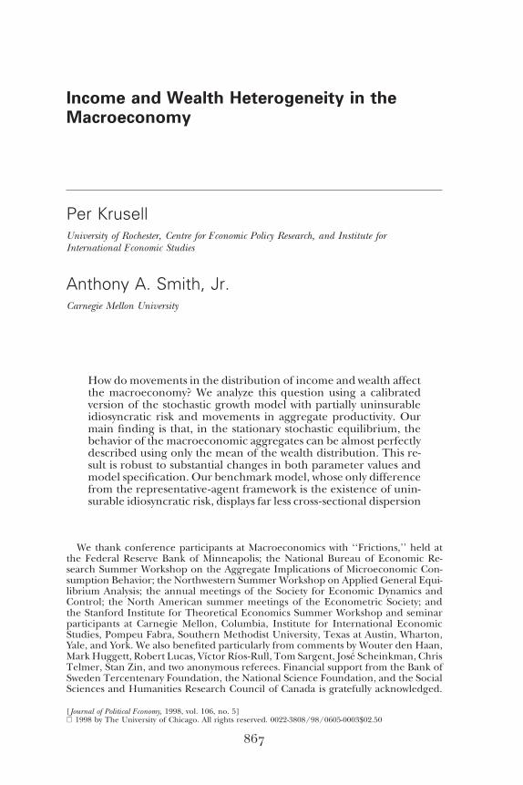
With a log-linear functional form and only the mean of the capitalstock as a state variable, we obtain the following approximate equilib-rium,

log k ′ 5 0.095 1 0.962 log k ; R 2 5 .999998, σ 5 0.0028%,

in good times and

log k ′ 5 0.085 1 0.965 log k ; R 2 5 .999998, σ 5 0.0036%

in bad times.10 There are two measures of fit: R 2 and the standarddeviation (percent) of the regression error, σ. Using our simulatedsample (consisting of 10,000 observations), we plot tomorrow’s ag-

9 Our labor income process is similar to that in Imrohoroglu (1989).10 We also used a nonlinear flexible functional form for the law of motion, with

virtually identical results.


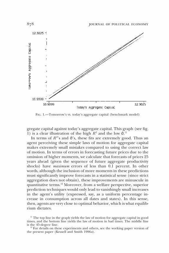
Fig. 1.—Tomorrow’s vs. today’s aggregate capital (benchmark model)

gregate capital against today’s aggregate capital. This graph (see fig.1) is a clear illustration of the high R 2 and the low σ.11

In terms of R 2’s and σ’s, these fits are extremely good. Thus anagent perceiving these simple laws of motion for aggregate capitalmakes extremely small mistakes compared to using the correct lawof motion. In terms of errors in forecasting future prices due to theomission of higher moments, we calculate that forecasts of prices 25years ahead (given the sequence of future aggregate productivityshocks) have maximum errors of less than 0.1 percent. In otherwords, although the inclusion of more moments in these predictionsmust significantly improve forecasts in a statistical sense (since strictaggregation does not obtain), these improvements are minuscule inquantitative terms.12 Moreover, from a welfare perspective, superiorprediction techniques would only lead to vanishingly small increasesin the agent’s utility (expressed, say, as a uniform percentage in-crease in consumption across all dates and states). In this sense,then, agents are very close to optimal behavior, which is what equilib-rium dictates.

11 The top line in the graph yields the law of motion for aggregate capital in goodtimes, and the bottom line yields the law of motion in bad times. The middle lineis the 45-degree line.

12 For details on these experiments and others, see the working paper version ofthe present paper (Krusell and Smith 1996a).


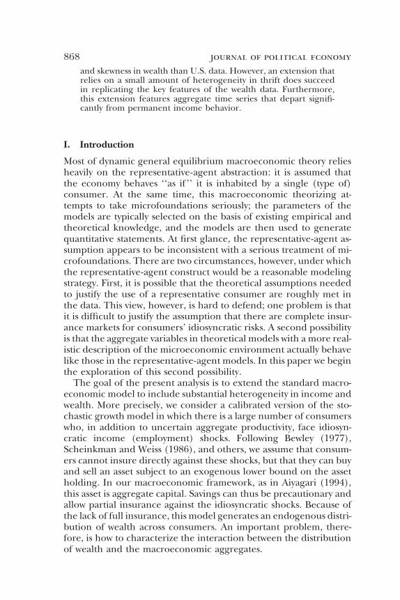
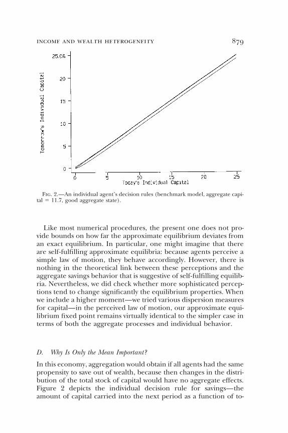
Fig. 2.—An individual agent’s decision rules (benchmark model, aggregate capi-tal 5 11.7, good aggregate state).

Like most numerical procedures, the present one does not pro-vide bounds on how far the approximate equilibrium deviates froman exact equilibrium. In particular, one might imagine that thereare self-fulfilling approximate equilibria: because agents perceive asimple law of motion, they behave accordingly. However, there isnothing in the theoretical link between these perceptions and theaggregate savings behavior that is suggestive of self-fulfilling equilib-ria. Nevertheless, we did check whether more sophisticated percep-tions tend to change significantly the equilibrium properties. Whenwe include a higher moment—we tried various dispersion measuresfor capital—in the perceived law of motion, our approximate equi-librium fixed point remains virtually identical to the simpler case interms of both the aggregate processes and individual behavior.

D. Why Is Only the Mean Important?

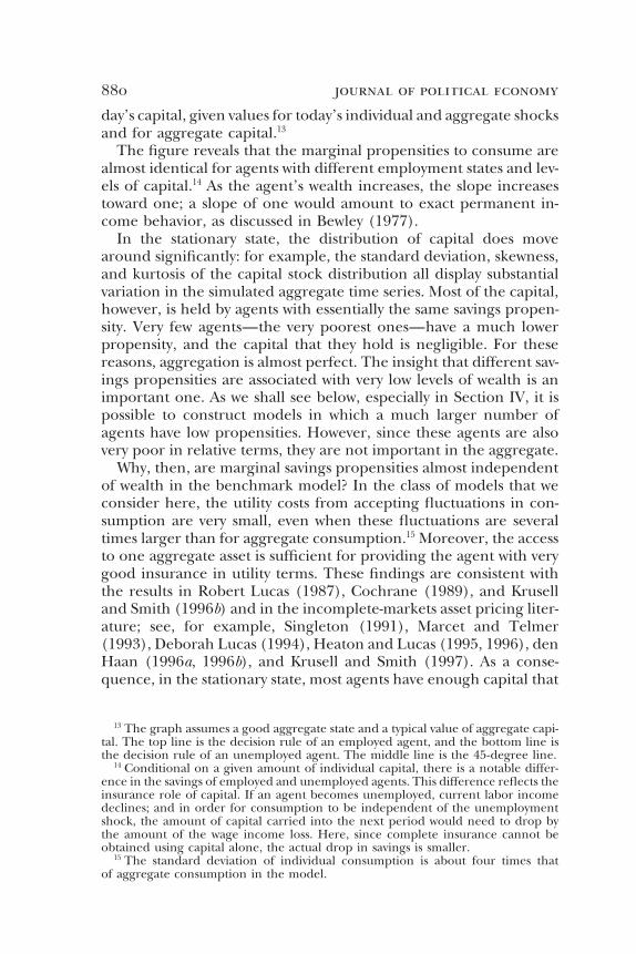
In this economy, aggregation would obtain if all agents had the samepropensity to save out of wealth, because then changes in the distri-bution of the total stock of capital would have no aggregate effects.Figure 2 depicts the individual decision rule for savings—theamount of capital carried into the next period as a function of to-


day’s capital, given values for today’s individual and aggregate shocksand for aggregate capital.13

The figure reveals that the marginal propensities to consume arealmost identical for agents with different employment states and lev-els of capital.14 As the agent’s wealth increases, the slope increasestoward one; a slope of one would amount to exact permanent in-come behavior, as discussed in Bewley (1977).

In the stationary state, the distribution of capital does movearound significantly: for example, the standard deviation, skewness,and kurtosis of the capital stock distribution all display substantialvariation in the simulated aggregate time series. Most of the capital,however, is held by agents with essentially the same savings propen-sity. Very few agents—the very poorest ones—have a much lowerpropensity, and the capital that they hold is negligible. For thesereasons, aggregation is almost perfect. The insight that different sav-ings propensities are associated with very low levels of wealth is animportant one. As we shall see below, especially in Section IV, it ispossible to construct models in which a much larger number ofagents have low propensities. However, since these agents are alsovery poor in relative terms, they are not important in the aggregate.

Why, then, are marginal savings propensities almost independentof wealth in the benchmark model? In the class of models that weconsider here, the utility costs from accepting fluctuations in con-sumption are very small, even when these fluctuations are severaltimes larger than for aggregate consumption.15 Moreover, the accessto one aggregate asset is sufficient for providing the agent with verygood insurance in utility terms. These findings are consistent withthe results in Robert Lucas (1987), Cochrane (1989), and Kruselland Smith (1996b) and in the incomplete-markets asset pricing liter-ature; see, for example, Singleton (1991), Marcet and Telmer(1993), Deborah Lucas (1994), Heaton and Lucas (1995, 1996), denHaan (1996a, 1996b), and Krusell and Smith (1997). As a conse-quence, in the stationary state, most agents have enough capital that

13 The graph assumes a good aggregate state and a typical value of aggregate capi-tal. The top line is the decision rule of an employed agent, and the bottom line isthe decision rule of an unemployed agent. The middle line is the 45-degree line.

14 Conditional on a given amount of individual capital, there is a notable differ-ence in the savings of employed and unemployed agents. This difference reflects theinsurance role of capital. If an agent becomes unemployed, current labor incomedeclines; and in order for consumption to be independent of the unemploymentshock, the amount of capital carried into the next period would need to drop bythe amount of the wage income loss. Here, since complete insurance cannot beobtained using capital alone, the actual drop in savings is smaller.

15 The standard deviation of individual consumption is about four times thatof aggregate consumption in the model.


their savings behavior is guided mainly by intertemporal concernsrather than by insurance motives. The availability of enough capitalis automatic here since our model has a neoclassical productionfunction with high marginal returns to capital at low levels of capitaland a realistic capital/output ratio.

E. Robustness

We performed a large number of sensitivity checks by changing pa-rameter values within the context of the benchmark specification.The working paper version of this paper (Krusell and Smith 1996a)documents these experiments in detail. The basic finding from theseexperiments is that it is extremely difficult to find exceptions to theapproximate aggregation result. For example, if individual shocksare more volatile or more persistent (alternatively, if borrowing ismore restricted or if agents are more risk averse), the aggregateeconomy responds by accumulating just enough extra capital to pro-vide most agents with a large enough buffer that the shocks do nothurt them much in utility terms.

Experiments with the discount rate deserve special mention: weobserve that more impatience leads to lower propensities to con-sume on average and to more dispersion in marginal propensities.There is an explicit connection to Bewley’s (1977) work here.16 Bew-ley considers a decision-theoretic framework with an agent facingincome risk and a sure return to savings of unity. He shows that asthe agent’s discount factor approaches unity and as the agent’s ini-tial wealth grows larger, the agent’s savings function becomes linearwith a slope of unity—permanent income behavior. In our econ-omy, if we were to let the discount rate and the depreciation rate(β, δ) approach (1, 0), the capital stock would increase to infinityand the gross rate of return on savings would become unity, thusplacing the agent in a situation identical to the limit that Bewleyconsiders. Our computations indeed show that higher discount ratesstrengthen (and lower discount rates weaken) the aggregation re-sult. However, large decreases in β are necessary in order for thegoodness of fit to significantly worsen; for example, the percentagestandard deviation of the regression error is only about 10 timeshigher for a β as low as 0.67.

We also considered models with valued leisure, various forms ofheterogeneity in preferences (risk aversion and patience), and fixedcosts of adjusting capital, and our main finding holds up in these

16 We thank Jose Scheinkman for drawing our attention to the connection betweenour setup and that studied by Bewley.


extensions as well. The valued-leisure (‘‘real business cycle’’) exten-sion is especially interesting since it complicates the determinationof prices: wages and rental rates no longer depend only on aggregatecapital and the aggregate shock, but also on the total work effort.17

With significant dependence of individual work effort on wealth,thus, aggregation might fail. However, it turns out that even in aformulation with large wealth effects, the relation between wealthand effort is almost linear for most agents. Thus our approximateaggregation result continues to hold in a model with valued leisure.The Appendix contains a more detailed description of this model.

IV. Matching the Wealth Distribution

Is the benchmark model of the last section a reasonable model ofincome and wealth heterogeneity? The labor income process is verysimple, but it is calibrated so as to at least roughly match incomevariability due to employment variation. Heterogeneity in wealth,however, is entirely nontrivially determined. As it turns out, oneproblem with the present model is that it does not generate realisticwealth heterogeneity: the data display significantly more skewnessfor wealth than the model does.18 More precisely, too few agents holdlow levels of wealth, and the concentration of wealth among the rich-est agents is far too small. On the basis of data in Wolff (1994) andDıaz-Gimenez, Quadrini, and Rıos-Rull (1997), for example, thepoorest 20 percent of the population have about zero wealth on aver-age, whereas the richest 5 percent of the population hold roughlyhalf of all the wealth. In contrast, the benchmark model predictsthat the poorest 20 percent hold (on average) 9 percent of totalwealth whereas the richest 5 percent hold (on average) 11 percent:there is significant skewness, but not nearly as much as in the data.

One of the main purposes of our line of research is to extend thestandard macroeconomic framework to allow heterogeneity amongconsumers. Therefore, it seems important to make sure that the het-erogeneity in the new framework is quantitatively adequate. In thissection we construct one model that roughly matches the observedincome and wealth distributions. We show that the approximate ag-gregation result still obtains in this model, and we go on to make a

17 In separate work (Krusell and Smith 1997) we consider an extension with an-other nontrivial market: a market for a riskless bond. Approximate aggregation alsoobtains in that setup.

18 This is also true for similar frameworks that have richer processes for laborincome than we do (see, e.g., Aiyagari 1994; Huggett 1996; Castaneda, Dıaz-Gimenez, and Rıos-Rull, in press): for a given, realistic, labor income distribution,there is far too little skewness in wealth.


few remarks about how this model compares to the standard repre-sentative-agent framework.

Amending the model to generate a large group of poor agents isstraightforward. For example, one can follow Hubbard, Skinner, andZeldes (1995) in assuming realistic settings for taxes, subsidies, andsocial insurance at low levels of income, which they show impliesthat low-income agents have incentives not to save. In addition, equi-librium frameworks with overlapping generations of consumers whoare not altruistically linked, as studied in Huggett (1996), tend togenerate stationary wealth distributions with more agents close tozero wealth. We follow the former of these routes, although in astylistic fashion: we assume that unemployed agents receive incometoo. We set their income to a number that is about 9 percent of theaverage employed wage. In this case, agents are less afraid of havinglow asset holdings since their compensation when unemployed nowserves as partial insurance. At the same time, we set the lower boundon capital holdings to a negative number rather than zero. That is,we allow agents to borrow, with maximum allowable borrowings be-ing set at about half of average annual earnings.19

To find assumptions that lead to a long (thick) right tail is harder;it seems necessary either to make rich agents have higher propensi-ties to save or to give them higher returns on saving (or both). Quad-rini (1996) and Quadrini and Rıos-Rull (1996) do the latter, whereaswe explore a setting with preference heterogeneity. In particular,we assume that agents’ preferences are ex ante identical but thatdiscount factors are random and follow a Markov process. Of course,there are no direct observations on discount factors, but we thinkthat it is reasonable to assume some heterogeneity across genera-tions within a dynasty (i.e., we do not have to assume that differentdynasties face different discount rate processes). We subject the ex-periment to the requirements (1) that the differences in discountfactors are not large and (2) that their distribution is symmetricaround its mean. More precisely, we assume that β can take on threevalues, 0.9858, 0.9894, and 0.9930, and that the transition probabili-ties are such that (i) the invariant distribution for β’s has 80 percentof the population at the middle β and 10 percent at each of theother β’s, (ii) immediate transitions between the extreme values ofβ occur with probability zero, and (iii) the average duration of thehighest and lowest β’s is 50 years. We choose the latter number toroughly match the length of a generation since we view the model

19 Specifically, we set the wage of an ‘‘unemployed’’ agent equal to 0.07 and weset the borrowing constraint equal to 22.4 (which is stricter than an always pay backconstraint).

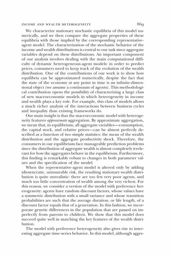
884 journal of political economyTABLE 1

Distribution of Wealth: Models and Data

Percentage of WealthHeld by Top

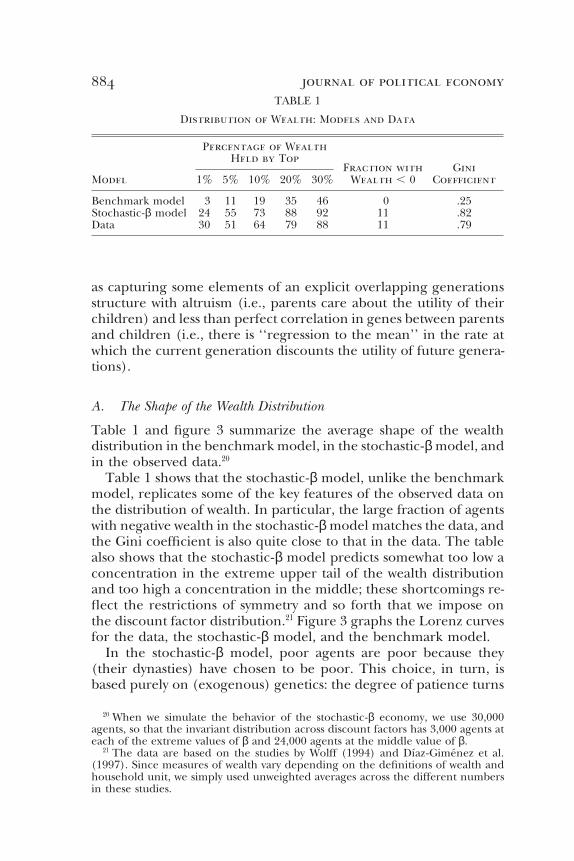
Fraction with GiniModel 1% 5% 10% 20% 30% Wealth , 0 Coefficient

Benchmark model 3 11 19 35 46 0 .25Stochastic-β model 24 55 73 88 92 11 .82Data 30 51 64 79 88 11 .79

as capturing some elements of an explicit overlapping generationsstructure with altruism (i.e., parents care about the utility of theirchildren) and less than perfect correlation in genes between parentsand children (i.e., there is ‘‘regression to the mean’’ in the rate atwhich the current generation discounts the utility of future genera-tions).

A. The Shape of the Wealth Distribution

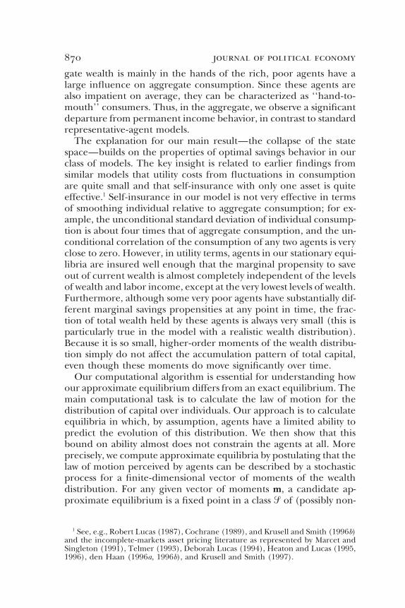
Table 1 and figure 3 summarize the average shape of the wealthdistribution in the benchmark model, in the stochastic-β model, andin the observed data.20

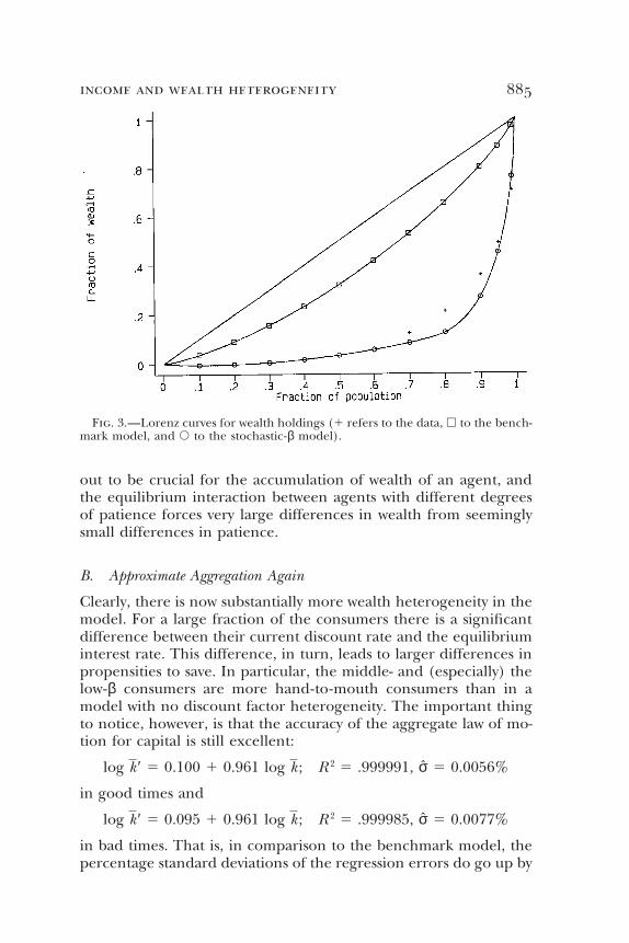
Table 1 shows that the stochastic-β model, unlike the benchmarkmodel, replicates some of the key features of the observed data onthe distribution of wealth. In particular, the large fraction of agentswith negative wealth in the stochastic-β model matches the data, andthe Gini coefficient is also quite close to that in the data. The tablealso shows that the stochastic-β model predicts somewhat too low aconcentration in the extreme upper tail of the wealth distributionand too high a concentration in the middle; these shortcomings re-flect the restrictions of symmetry and so forth that we impose onthe discount factor distribution.21 Figure 3 graphs the Lorenz curvesfor the data, the stochastic-β model, and the benchmark model.

In the stochastic-β model, poor agents are poor because they(their dynasties) have chosen to be poor. This choice, in turn, isbased purely on (exogenous) genetics: the degree of patience turns

20 When we simulate the behavior of the stochastic-β economy, we use 30,000agents, so that the invariant distribution across discount factors has 3,000 agents ateach of the extreme values of β and 24,000 agents at the middle value of β.

21 The data are based on the studies by Wolff (1994) and Dıaz-Gimenez et al.(1997). Since measures of wealth vary depending on the definitions of wealth andhousehold unit, we simply used unweighted averages across the different numbersin these studies.


Fig. 3.—Lorenz curves for wealth holdings (1 refers to the data, h to the bench-mark model, and s to the stochastic-β model).

out to be crucial for the accumulation of wealth of an agent, andthe equilibrium interaction between agents with different degreesof patience forces very large differences in wealth from seeminglysmall differences in patience.

B. Approximate Aggregation Again

Clearly, there is now substantially more wealth heterogeneity in themodel. For a large fraction of the consumers there is a significantdifference between their current discount rate and the equilibriuminterest rate. This difference, in turn, leads to larger differences inpropensities to save. In particular, the middle- and (especially) thelow-β consumers are more hand-to-mouth consumers than in amodel with no discount factor heterogeneity. The important thingto notice, however, is that the accuracy of the aggregate law of mo-tion for capital is still excellent:

log k ′ 5 0.100 1 0.961 log k ; R 2 5 .999991, σ 5 0.0056%

in good times and

log k ′ 5 0.095 1 0.961 log k ; R 2 5 .999985, σ 5 0.0077%

in bad times. That is, in comparison to the benchmark model, thepercentage standard deviations of the regression errors do go up by

886 journal of political economyTABLE 2

Aggregate Time Series

StandardDeviation

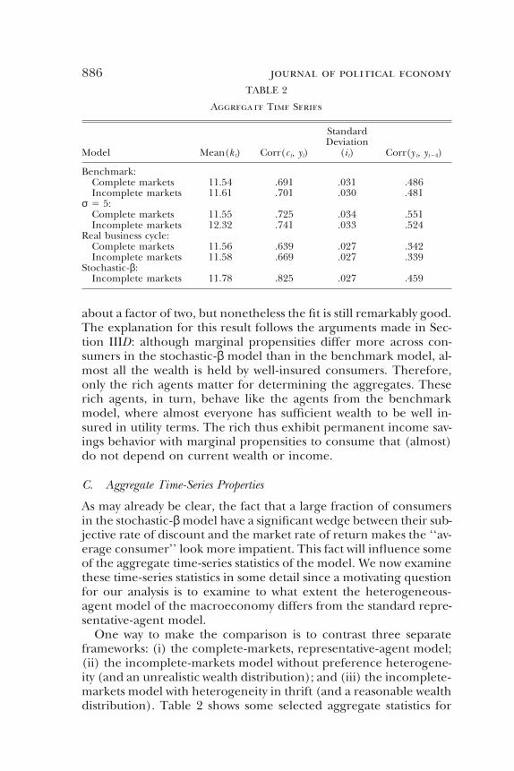
Model Mean(k t) Corr(c t, yt) (it) Corr(y t, yt24)

Benchmark:Complete markets 11.54 .691 .031 .486Incomplete markets 11.61 .701 .030 .481

σ 5 5:Complete markets 11.55 .725 .034 .551Incomplete markets 12.32 .741 .033 .524

Real business cycle:Complete markets 11.56 .639 .027 .342Incomplete markets 11.58 .669 .027 .339

Stochastic-β:Incomplete markets 11.78 .825 .027 .459

about a factor of two, but nonetheless the fit is still remarkably good.The explanation for this result follows the arguments made in Sec-tion IIID: although marginal propensities differ more across con-sumers in the stochastic-β model than in the benchmark model, al-most all the wealth is held by well-insured consumers. Therefore,only the rich agents matter for determining the aggregates. Theserich agents, in turn, behave like the agents from the benchmarkmodel, where almost everyone has sufficient wealth to be well in-sured in utility terms. The rich thus exhibit permanent income sav-ings behavior with marginal propensities to consume that (almost)do not depend on current wealth or income.

C. Aggregate Time-Series Properties

As may already be clear, the fact that a large fraction of consumersin the stochastic-β model have a significant wedge between their sub-jective rate of discount and the market rate of return makes the ‘‘av-erage consumer’’ look more impatient. This fact will influence someof the aggregate time-series statistics of the model. We now examinethese time-series statistics in some detail since a motivating questionfor our analysis is to examine to what extent the heterogeneous-agent model of the macroeconomy differs from the standard repre-sentative-agent model.

One way to make the comparison is to contrast three separateframeworks: (i) the complete-markets, representative-agent model;(ii) the incomplete-markets model without preference heterogene-ity (and an unrealistic wealth distribution); and (iii) the incomplete-markets model with heterogeneity in thrift (and a reasonable wealthdistribution). Table 2 shows some selected aggregate statistics for


these models.22 The table also covers two additional extensions ofthe benchmark model: one with a high value of risk aversion (σ 55) and one with valued leisure (the real business cycle model).

Two main kinds of observations can be made using table 2. First,the table allows an evaluation of the effects of market incom-pleteness. Second, the table makes it possible to gauge the effectsof introducing preference heterogeneity and, thus, a realistic wealthdistribution on the aggregate time series.

Table 2 shows that the lack of full insurance always raises thesteady-state aggregate capital stock since capital has the additionalvalue of insuring against risk. The amount of precautionary savingsfor the benchmark model is about 0.6 percent (calculated as thepercentage increase in the capital stock when insurance markets areclosed), which is quite small. However, with more risk-averse agents,the amount of precautionary savings rises significantly: with a degreeof relative risk aversion of five, the amount of precautionary savingsis 6.7 percent. The reason for the increase is apparent: the agentsin the economy increase their total buffer since being poorly insuredhurts more when agents are more risk-averse. In contrast, the realbusiness cycle model gives somewhat lower precautionary savingssince varying leisure allows a complementary way of adjusting con-sumption in response to shocks.

The incomplete-markets economies have second-moment prop-erties that are different from their representative-agent counter-parts, but not by large amounts. The difference is especially small forthe benchmark economy, which shows very small effects of marketincompleteness overall. In fact, this observation extends beyond theparticular moments reported in table 2: simulated realizations showthat the two market structures lead to virtually indistinguishable timeseries, except for the difference in means. In the setups with higherrisk aversion and valued leisure, the differences are somewhat larger.Overall, consumption tends to be a little more correlated with in-come when markets are incomplete, investment is slightly less vola-tile, and income is somewhat less serially correlated. In conclusion,in the models we examine that do not have preference heterogene-ity, the market structure matters only marginally for aggregate time-series behavior.

In the model with heterogeneity in thrift, what stands out most is

22 In table 2, k t denotes aggregate capital at time t, yt aggregate output, c t aggregateconsumption, and it aggregate investment. The statistics in the table are computedusing a simulated sample consisting of 11,000 observations, with the first 1,000 obser-vations discarded in order to diminish dependence on initial conditions. In orderto facilitate comparisons across models, we use the same sequence of aggregateshocks for all model economies when generating the simulated time series.


the consumption-output correlation. The large correlation reflectsthe hand-to-mouth behavior of the least patient (low-β) consumers.Although these impatient consumers have very little capital and,thus, matter little for what happens to the evolution of economywidewealth, their consumption behavior is a more significant part of thetotal; the most patient (high-β) consumers are much richer but con-sume more only by the amount of the interest payments on theirassets. In this model, the interest rate is slightly below the discountrate of the most patient agents (the difference arises since assetsto some extent are used for precautionary savings). The differencebetween the interest rate and the discount rate of the least patientagents, however, is larger. This larger wedge leads to a stronger de-parture from permanent income behavior. In fact, the correlationbetween the aggregate consumption of the least patient agents andaggregate output is (on average) .90 in this model; for the most pa-tient agents this correlation is .61.23

In a complete-markets setting in which all consumers have thesame discount rate, consumers exhibit permanent income behaviorregardless of the degree of their impatience (for reasonably cali-brated income processes): if the discount rate is lowered, the station-ary equilibrium interest rate adjusts so that the two remain very close.In contrast, in a model in which agents with different discount ratescoexist, departures from permanent income behavior arise natu-rally. An important related point is that the more impatient consum-ers in the incomplete-markets model do not smooth consumptionand thus also may give the impression of being up against a bor-rowing constraint. Although the borrowing constraint does indeedlimit consumption possibilities, the chief reason for impatientagents’ rush to consume is precisely that they are more impatientthan others. Empirically, it is not obvious how to distinguish a bind-ing borrowing constraint from a lower than average degree of pa-tience.

In sum, we find that the heterogeneous- and representative-agentversions of some of the models generate aggregate behavior withimportant similarities. We also find, however, that these similarities

23 We did not solve the complete-markets version of the multiple-β model (it doesnot aggregate). However, we did compare economies with two groups of agents,one with a permanently high β and one with a permanently low β, since the com-plete-markets version of such an economy does aggregate: in the stationary state,only the high-β agents are economically active. The effects of incomplete markets onsecond moments in this case are very large. For example, the consumption-outputcorrelation is .691 in the complete-markets version and .865 in the incomplete-markets version. Since the model with permanently different β’s for different agentsis quite similar to the stochastic-β model, in which β’s are highly persistent, theeffects of changing the market structure are likely similar for the stochastic-β model.


do not extend to all properties of the models nor to all the models.In addition, heterogeneity appears to be a key factor in generatingsome of the most prominent differences, such as the tendency of theaggregate, or average, consumer to depart from permanent incomebehavior. Although this departure is more marked in some of themodels than in others, it occurs in all the heterogeneous-agent mod-els that we study.

V. Concluding Remarks

In the Introduction to this paper we set out to investigate whetherrepresentative-agent models of the macroeconomy might be justi-fied by showing that models with consumer heterogeneity give riseto aggregate time series that are in fact close to those of the represen-tative-agent models. For this purpose, we studied a fairly rich classof neoclassical production economies with incomplete insurancemarkets for idiosyncratic risk and heterogeneity in income, wealth,and preferences. Our first and main finding is that a low-dimen-sional object—the total capital stock and the value of the aggregateproductivity shock—seems to be sufficient for characterizing the sto-chastic behavior of all the macroeconomic aggregates, despite sub-stantial heterogeneity in the population with respect to wealth aswell as to some preference parameters. Hence, one need track onlythe evolution of the ‘‘aggregate budget’’ in order to analyze the dy-namic behavior of the macroeconomic aggregates.

A natural question is thus whether it is possible to describe prefer-ences of an ‘‘aggregate consumer’’ such that when this agent’s utilityis maximized subject to the aggregate budget the outcome is a set oftime series that matches those calculated here. Our second finding isthat this is sometimes, but not always, an easy task. In our benchmarkeconomy and some extensions to it, the incomplete-markets (het-erogeneous-agent) economy behaves almost identically to its com-plete-markets (representative-agent) counterpart, except for a dif-ference in levels: in the stationary stochastic equilibrium, capital isslightly higher in the incomplete-markets version. In some exten-sions to the benchmark setup, however, especially those with prefer-ence heterogeneity, some second moments of the aggregate timeseries are substantially different. Although we have not explicitlytried to formulate preferences of a fictitious representative con-sumer whose behavior might match the aggregate consumption be-havior generated by the heterogeneous-agent models, it seems nec-essary to move outside the class of models with a single infinitelylived agent with time-additive preferences. In particular, in repre-sentative-agent models with time-additive preferences, it seems dif-


ficult to obtain the departures from permanent income behaviorthat we observe in the incomplete-markets models with heterogene-ity in preferences. In other words, the interaction of consumers withheterogeneous preferences in an incomplete-markets setting leadsto new insights. Among the models we study, those that come theclosest to matching real-world wealth distributions are preciselymodels with heterogeneous preferences and incomplete markets.

An important task is to investigate further the robustness of ourfindings. First, it would be interesting to know whether life cyclesavings motives might lead to different results. Rıos-Rull (1996)shows that calibrated life cycle models without altruism but withcomplete markets generate aggregate behavior that is very similarto that of the benchmark (or real business cycle) model studied inthis paper. These results suggest that life cycle considerations alonedo not lead to significant departures from permanent income behav-ior on the part of individual consumers. An open question is whetherintroducing incomplete markets into a life cycle model would besufficient to generate significant departures from permanent in-come behavior on the part of individual consumers.24 Second, mod-els with endogenous borrowing constraints, such as in Kiyotaki andMoore (1997), might ascribe a more important role to the distribu-tion of wealth. Third, one simple extension of the standard growthmodel that may give rise to stronger effects from the distribution ofcapital is to force consumers to use their own production technolo-gies (in contrast to our setup in which the return to savings is equalfor all agents). Finally, as Banerjee and Newman (1993) have shown,fixed costs in capital accumulation may also lead to a more funda-mental dependence of the aggregates on the distribution of re-sources across agents.

Although not in main focus in this paper, how the state of themacroeconomy and macroeconomic policy shape the distributionof consumption and wealth is an important question, at least judgingfrom contemporary public debate. The methodological findings inthis paper suggest that such issues can be feasibly studied: it nowseems within our ability to begin using equilibrium models to ana-lyze the interrelation between business cycles, inequality, and eco-nomic policy. In this context, an important task is to analyze furtherthe determinants of the wealth distribution. As we have shown inthis paper, introducing preference heterogeneity into the standardmodel allows a closer match between model and data. It is necessary,however, to consider carefully other hypotheses as well. The use of

24 Storesletten, Telmer, and Yaron (1996) investigate a life cycle model with incom-plete markets and persistent idiosyncratic shocks.


household data should prove fruitful for comparing competinghypotheses.

Appendix

A. Numerical Solution Method for the Agent’s Problem

This Appendix describes the numerical techniques used to solve the con-sumer’s dynamic programming problem. The algorithm is similar to oneused in Johnson et al. (1993). The description here assumes that we aresolving the benchmark economy. In addition, it assumes that only one mo-ment of the capital distribution (i.e., k) is included in the law of motionfor aggregate capital. It is straightforward to modify the algorithm so as toaccommodate a different model specification or additional moments.25

The objective of the numerical algorithm is to approximate the four func-tions v(k, 1; k, z g), v(k, 1; k, z b), v(k, 0; k, z g), and v(k, 0; k, z b). We accomplishthis task by approximating the values of each of these functions on acoarse grid of points in the (k, k) plane and then using cubic spline andpolynomial interpolation to calculate the values of these functions at pointsnot on the grid. The numerical algorithm is in many ways analogous tovalue function iteration, except we do not restrict choices for capital topoints on the grid.

The following steps describe the numerical procedure. (1) Choose a gridof points in the (k, k) plane (we give some details below about how wechoose these points). (2) Choose initial values for each of the four functionsat each of the grid points. (It is generally feasible to use the zero functionas the initial condition for each of the functions.) (3) For each of the four(z, e) pairs, maximize the right-hand side of Bellman’s equation at eachpoint in the grid. In this maximization, we allow the agent to select anyvalue for capital. We use various interpolation schemes to compute thevalue function at points not on the grid (we describe the interpolationschemes in greater detail below). For large values of k (i.e., values for whichthe borrowing constraint does not bind), we use a Newton-Raphson proce-dure for finding the optimal choice of capital. For small values of k (i.e.,for values close to the borrowing constraint), we use a bisection procedureto map out the objective function. This procedure allows for the possibilitythat the borrowing constraint binds (in which case the optimal value ofcapital is at a corner, so that the first derivative of the objective function isnot zero at the optimum). (4) Compare the new optimal values generatedby step 3 to the original values. If the new values are close to the old values,then stop; otherwise, repeat step 3 until the new and old values are suffi-ciently close. (In practice, value functions typically converge more slowlythan the decision rules associated with these value functions. Thus it is gen-erally more efficient to stop the iterations when the optimal decisions at

25 There are many available methods for solving the class of decision problemsthat we consider in this paper. We have chosen a method that we find to be robustto changes in model specification and that allows us to achieve high accuracy.


each of the grid points stop changing, even if the value functions have notyet fully converged.)

We now comment on the choice of a grid in the (k, k) plane and onthe interpolation schemes that we use. Since there is generally not muchcurvature in the value function in the k direction, we use a small numberof grid points in this direction and we use polynomial interpolation to com-pute the value function for values of k not on the grid. If there are n pointsin the k direction, then polynomial interpolation fits a polynomial of ordern 2 1 to the function values at these points (so that the polynomial fits thevalues exactly). This polynomial is then used to compute the value functionin between grid points. We compute the value of the interpolating polyno-mial using Neville’s algorithm, as described in Press et al. (1989, chap. 3).This algorithm avoids the numerical instabilities associated with computingthe coefficients of the interpolating polynomial. We generally use four tosix equally spaced points in the k direction.

In the k direction, there is generally a fair amount of curvature in thevalue function, especially for values of k near the borrowing constraint. Inthis direction, therefore, we use cubic spline interpolation, which fits apiecewise cubic function through the given function values, with one piecefor each interval defined by the grid. This piecewise cubic function satisfiesthe following restrictions: (1) it matches the function values exactly at thegrid points, and (2) its first and second derivatives are continuous at thegrid points. Cubic splines can be computed efficiently by solving a set oftridiagonal linear equations (see, e.g., the description in Press et al. [1989,chap. 3] or de Boor [1978, chap. 4]). Computing cubic splines requiresthe imposition of two side conditions: we impose that the second derivativeof the value function at the first grid point for k is slightly smaller than thesecond derivative at the second grid point and that the second derivativeat the last grid point is slightly larger than at the next to last grid point.We generally use 70–130 grid points in the k direction, with many gridpoints near zero (where there is a lot of curvature) and fewer grid pointsfor larger values of k (where there is less curvature). We find that our resultsare not sensitive to increasing the number of grid points in either the k ork direction.

To combine these two interpolation schemes, we therefore proceed asfollows, where m is the number of grid points in the k direction. (1) Foreach of the m values of k, use polynomial interpolation to compute thevalue function at the desired value of k′. This set of interpolations yields mvalues of the value function, one for each value of k in the grid. (2) Usecubic spline interpolation using the m interpolated values to calculate thevalue function for values of k that are not on the grid. Since the values ofk ′ at which interpolated values must be computed are known at the begin-ning of each of the iterations on the value function, the required cubicsplines need to be computed only once for each iteration.

In order to simulate the behavior of agents, we need to approximate thedecision rules associated with the approximate value function as computedabove. (Since these decision rules in general need to be evaluated at many


different values of k in the course of simulating the dynamic behavior ofthe economy, it is not efficient to use the interpolation scheme de-scribed above to compute optimal decisions at points not on the grid.) Weapproximate the decision rules by first computing optimal decisions on afine grid of points in the (k, k) plane for each value of (z, e). When comput-ing these optimal decisions, we use the approximate value function as com-puted above. For the purpose of approximating decision rules, we generallyuse 150–600 equally spaced points in the k direction and 25–100 equallyspaced points in the k direction. Optimal decisions at points not on the gridare then computed using bilinear interpolation (see Press et al. 1989, chap.3). To conserve on computation time, the coefficients determining the bi-linear interpolation need to be computed only once, prior to simulatingthe behavior of the economy. Given these coefficients and an efficientmethod for finding the appropriate location in the two-dimensional (k, k)grid, it is quick and easy to compute individual savings decisions.

As a final point, it is important to ensure that simulations of the econo-my’s behavior impose the law of large numbers (or at least its first-momentimplications). In particular, it is important to make sure that the fractionof unemployed agents is exactly u g in good times and u b in bad times. Toaccomplish this task in the simulated data, we first update the employmentstatus of each agent according to the appropriate conditional probabilities.We then check to see whether the fraction of unemployed agents matchesthe desired number. If, for example, there are too many employed agents,we choose an employed agent at random, switch his employment status tounemployed, and then continue this process until the fraction of employedagents matches the desired number.

B. The Model with Valued Leisure

Assume that time spent off work, 1 2 l, where l is the amount of laborsupplied, is valued according to

U(c, l ) 5 limν →σ

[cθ(1 2 l )12θ]12ν 2 11 2 ν

,

where we set σ to one and θ to 1/2.9. In our recursive equilibrium defini-tion, there is now an additional element to consider: the way in which lei-sure is supplied at each point in time. Let the aggregate amount of hoursworked be given by the function L: l 5 L(Γ, z). This function is needed asan input in each agent’s decision; to know prices, l needs to be determined,and this is what L delivers. Optimal decisions of the agent thus lead to thedecision rule l 5 g(k, e; Γ, z) specifying how much to work at each valueof the state. The equilibrium condition for L thus states that at any givenstate (Γ, z), L(Γ, z) equals the total labor supply when integrated over thepopulation using individual supplies given by g.

When we approximate the aggregate labor supply function as a log-linearfunction of the total stock of capital, our results are as follows:

894 journal of political economylog k ′ 5 0.123 1 0.951 log k ; R 2 5 .999994, σ 5 0.0040%,

log l 5 20.544 2 0.252 log k ; R 2 5 .992, σ 5 0.039%

in good times and

log k ′ 5 0.114 1 0.953 log k ; R 2 5 .999993, σ 5 0.0049%,log l 5 20.592 2 0.255 log k ; R 2 5 .988, σ 5 0.054%

in bad times.26 The fit is still very good for the law of motion for capital.For the aggregate labor function, the fit is good, but not as good as for thelaw of motion of capital: the R 2’s are lower, and in contrast to figure 1,there are noticeable ‘‘clouds’’ in a graph of aggregate labor supply againstaggregate capital (the working paper version of this paper [Krusell andSmith 1996a] displays this graph).

Just as for the savings decision, the nonlinearities in the agent’s decisionrule for labor are stronger at low levels of capital (the marginal propensityto take leisure is higher for poor agents). These nonlinearities, togetherwith the fact that poor agents supply a disproportionately large amount ofaggregate labor, account for the ‘‘clouds’’ in a graph of aggregate laboragainst aggregate capital. The fit, however, is very good: although it is possi-ble to detect a decrease in forecasting accuracy as compared to the bench-mark model, the changes are minor. Our assumption that utility is Cobb-Douglas in consumption and leisure clearly works against aggregation; sincepoor agents work harder than rich agents in the model, the nonlinearitiesin the decision rule for leisure receive high weight. A preference assump-tion with no wealth effects—a nesting of the kind c 1 (1 2 l )γ—wouldimprove the fit significantly.27 Similarly, if employed agents are allowed tohave different labor productivities, those with higher productivity wouldwork more and be richer, leading to significantly smaller ‘‘clouds’’ and im-proved fits. Further, extensions to include human capital accumulationwould tend to lead to a positive correlation between financial and humancapital. This extension would give poor agents a low weight in the totalsupply of effective labor units and, thus, diminish the effects of the nonline-arities. In fact, these alternative setups seem more consistent with observedpatterns for hours worked and relative wages. We chose our specificationmainly to illustrate that, despite assumptions that work against aggregation,the results are close to those of the benchmark setup.

26 We also computed an approximate equilibrium using two moments of the capi-tal stock distribution: its mean and its standard deviation. In this case, both the lawof motion for aggregate capital and the aggregate labor supply function depend onboth of these moments. Including an additional moment leads to significantly betterfits for the aggregate labor functions: in good times, R 2 5 .998 (σ 5 0.021 percent),and in bad times, R 2 5 .993 (σ 5 0.039 percent). In addition, the fit of the law ofmotion for aggregate capital improves slightly. The aggregate time series, however,are virtually unchanged.

27 This kind of formulation has been used in Greenwood, Hercowitz, and Huffman(1988).

income and wealth heterogeneity 895References

Aiyagari, S. Rao. ‘‘Uninsured Idiosyncratic Risk and Aggregate Saving.’’Q.J.E. 109 (August 1994): 659–84.

Aiyagari, S. Rao, and Gertler, Mark. ‘‘Asset Returns with Transactions Costsand Uninsured Individual Risk.’’ J. Monetary Econ. 27 ( June 1991): 311–31.

Banerjee, Abhijit V., and Newman, Andrew F. ‘‘Occupational Choice andthe Process of Development.’’ J.P.E. 101 (April 1993): 274–98.

Bewley, Truman F. ‘‘The Permanent Income Hypothesis: A Theoretical For-mulation.’’ J. Econ. Theory 16 (December 1977): 252–92.

Castaneda, A.; Dıaz-Gimenez, Javier; and Rıos-Rull, Jose-Victor. ‘‘Unem-ployment Spells, Cyclically Moving Factor Shares, and Income Distribu-tion Dynamics.’’ J. Monetary Econ. (in press).

Chatterjee, Satyajit. ‘‘Transitional Dynamics and the Distribution of Wealthin a Neoclassical Growth Model.’’ J. Public Econ. 54 (May 1994): 97–119.

Cochrane, John H. ‘‘The Sensitivity of Tests of the Intertemporal Allocationof Consumption to Near-Rational Alternatives.’’ A.E.R. 79 (June 1989):319–37.

de Boor, Carl. A Practical Guide to Splines. New York: Springer-Verlag, 1978.den Haan, Wouter J. ‘‘Heterogeneity, Aggregate Uncertainty, and the

Short-Term Interest Rate.’’ J. Bus. and Econ. Statis. 14 (October 1996):399–411. (a)

———. ‘‘Understanding Equilibrium Models with a Small and a LargeNumber of Agents.’’ Discussion Paper no. 96-34. La Jolla: Univ. Califor-nia, San Diego, 1996. (b)

Dıaz-Gimenez, Javier; Prescott, Edward C.; Fitzgerald, T.; and Alvarez, Fer-nando. ‘‘Banking in Computable General Equilibrium Economies.’’ J.Econ. Dynamics and Control 16 (July–October 1992): 533–59.

Dıaz-Gimenez, Javier; Quadrini, Vincenzo; and Rıos-Rull, Jose-Victor. ‘‘Di-mensions of Inequality: Facts on the U.S. Distributions of Earnings, In-come, and Wealth.’’ Fed. Reserve Bank Minneapolis Q. Rev. 21 (Spring1997): 3–21.

Dıaz-Gimenez, Javier, and Rıos-Rull, Jose-Victor. ‘‘Heterogeneous Agents,Capital Accumulation, and Business Cycles.’’ Manuscript. Philadelphia:Univ. Pennsylvania, 1991.

Greenwood, Jeremy; Hercowitz, Zvi; and Huffman, Gregory. ‘‘Investment,Capacity Utilization, and the Real Business Cycle.’’ A.E.R. 78 (June 1988):402–17.

Heaton, John, and Lucas, Deborah J. ‘‘The Importance of Investor Hetero-geneity and Financial Market Imperfections for the Behavior of AssetPrices.’’ Carnegie-Rochester Conf. Ser. Public Policy 42 (June 1995): 1–32.

———. ‘‘Evaluating the Effects of Incomplete Markets on Risk Sharing andAsset Pricing.’’ J.P.E. 104 (June 1996): 443–87.

Hubbard, R. Glenn; Skinner, Jonathan; and Zeldes, Stephen P. ‘‘Precau-tionary Saving and Social Insurance.’’ J.P.E. 103 (April 1995): 360–99.

Huggett, Mark. ‘‘The Risk-Free Rate in Heterogeneous-Agent Incomplete-Insurance Economies.’’ J. Econ. Dynamics and Control 17 (September–November 1993): 953–69.

———. ‘‘Wealth Distribution in Life-Cycle Economies.’’ J. Monetary Econ.38 (December 1996): 469–94.

896 journal of political economyI·mrohoroglu, Ayse. ‘‘Cost of Business Cycles with Indivisibilities and Liquid-

ity Constraints.’’ J.P.E. 97 (December 1989): 1364–83.———. ‘‘The Welfare Cost of Inflation under Imperfect Insurance.’’ J.

Econ. Dynamics and Control 16 (January 1992): 79–91.Johnson, Sharon A.; Stedinger, Jerry R.; Shoemaker, Christine A.; Li, Ying;

and Tejada-Guibert, Jose Alberto. ‘‘Numerical Solution of Continuous-State Dynamic Programs Using Linear and Spline Interpolation.’’ Opera-tions Res. 41 (May–June 1993): 484–500.

Kiyotaki, Nobuhiro, and Moore, John. ‘‘Credit Cycles.’’ J.P.E. 105 (April1997): 211–48.

Krusell, Per, and Rıos-Rull, Jose-Victor. ‘‘On the Size of U.S. Government:Political Economy in the Neoclassical Growth Model.’’ Manuscript. Roch-ester, N.Y.: Univ. Rochester, 1997.

Krusell, Per, and Smith, Anthony A., Jr. ‘‘Income and Wealth Heterogeneityin the Macroeconomy.’’ Working Paper no. 399. Rochester, N.Y.: Univ.Rochester, Center Econ. Res.; Working Paper no. 1997-37. Pittsburgh:Carnegie Mellon Univ., 1996. (a)

———. ‘‘Rules of Thumb in Macroeconomic Equilibrium: A QuantitativeAnalysis.’’ J. Econ. Dynamics and Control 20 (April 1996): 527–58. (b)

———. ‘‘Income and Wealth Heterogeneity, Portfolio Choice, and Equilib-rium Asset Returns.’’ Macroeconomic Dynamics 1, no. 2 (1997): 387–422.

Lucas, Deborah J. ‘‘Asset Pricing with Undiversifiable Income Risk andShort Sales Constraints: Deepening the Equity Premium Puzzle.’’ J. Mone-tary Econ. 34 (December 1994): 325–41.

Lucas, Robert E., Jr. Models of Business Cycles. New York: Blackwell, 1987.Marcet, Albert, and Singleton, Kenneth J. ‘‘Equilibrium Asset Prices and

Savings of Heterogeneous Agents in the Presence of Incomplete Marketsand Portfolio Constraints.’’ Manuscript. Barcelona: Univ. Pompeu Fabra,1991.

Press, William H.; Flannery, Brian P.; Teukolsky, Saul A.; and Vetterling,William T. Numerical Recipes: The Art of Scientific Computing. Cambridge:Cambridge Univ. Press, 1989.

Quadrini, Vincenzo. ‘‘Entrepreneurship, Saving, and Social Mobility.’’Ph.D. dissertation, Univ. Pennsylvania, 1996.

Quadrini, Vincenzo, and Rıos-Rull, Jose-Victor. ‘‘Models of the Distributionof Income, Wealth and Earnings.’’ Staff report. Minneapolis: Fed. Re-serve Bank, Res. Dept., 1996.

Rıos-Rull, Jose-Victor. ‘‘Life-Cycle Economies and Aggregate Fluctua-tions.’’ Rev. Econ. Studies 63 (July 1996): 465–89.

Scheinkman, Jose A., and Weiss, Laurence. ‘‘Borrowing Constraints andAggregate Economic Activity.’’ Econometrica 54 (January 1986): 23–45.

Storesletten, Kjetil; Telmer, Chris I.; and Yaron, Amir. ‘‘Persistent Idiosyn-cratic Shocks and Incomplete Markets.’’ Manuscript. Pittsburgh: Carne-gie Mellon Univ., 1996.

Telmer, Chris I. ‘‘Asset-Pricing Puzzles and Incomplete Markets.’’ J. Finance48 (December 1993): 1803–32.

Wolff, Edward N. ‘‘Trends in Household Wealth in the United States, 1962–83 and 1983–89.’’ Rev. Income and Wealth 40 (June 1994): 143–74.

Documents

Income and Wealth Heterogeneity in the Macroeconomy · Anthony A. Smith, Jr. ... We characterize stationary stochastic equilibria of this model nu-merically, and we then compare the