OECD (2012) www.oecd.org/social/inequality.htm

1

(Revised version: 18th February 2013)

INCOME DISTRIBUTION DATA REVIEW – ITALY1

1. Available data sources used for reporting on income inequality and poverty

1.1. OECD reporting:

OECD data on income inequality and poverty data for Italy refer to 1984, 1991, 1993, 1995, 2000,

2004, 2006, 2007, 2008 and 2009. These estimates are based on different data sources.

From 1984 to 1993, OECD estimates were based on data the micro-simulation model

ITAXMOD95, based on the Survey on Household Income and Wealth (SHIW), conducted by

the Bank of Italy.

From 1995 to 2004, OECD estimates were based the micro-simulation model MASTRICT,

maintained at ISTAT, and also based on the data from the Survey on Household Income and

Wealth (SHIW). Both micro-simulation models integrated the original survey records with

imputations on taxes paid by households (information on which was not available in SHIW)

but, in the process, also altered some of the values on market income. Data from this model

were also provided for the income year 2008.

From 2006 onwards (survey year: 2007 onwards), OECD estimates have been based on the

EU Survey on Income and Living Conditions (EU-SILC).

Therefore, several breaks need to be taken into consideration when reporting OECD time-series data.

First, a break in 1995 (due to the change in the micro-simulation model). Second, a break in 2006 (due to

the switch to EU-SILC survey). These two breaks are highlighted in the different graphs presented below.

The OECD Secretariat has addressed these breaks through multiplicative adjustments in 2006; while no

adjustment is made for 1993-1995, on account of the fact that estimates based on the two micro-simulation

models for adjacent years are very close to each other.

Please note that in the OECD database, several data may be provided for the same year. The following

‘flags’ are included in the database:

- Data labelled as “old” are those based on the ITAXMOD95 micro-simulation model;

- Data labelled as “previous” are those based on the MASTRICT micro-simulation model;

- Data labelled as “current” refer to EU-SILC data from 2006 onwards, while data for previous

years are based on backward interpolation from the current EU-SILC series in order to have a

consistent long time-series of data. Backward interpolation was based on the MASTRICT micro-

1 This revised version of this “Income Distribution review – Italy” benefited from valuable comments from Gaetano

Proto, ISTAT.

OECD (2012) www.oecd.org/social/inequality.htm

2

simulation model for the years 2006 to 1995; and on the ITAXMOD95 micro-simulation model

for years from 1993 to 1984.

Evidence in this Review is based on the OECD “Current” data for better consistency over time.

1.2. National reporting and reporting in other international agencies:

The following datasets are available for Italy:

The Bank of Italy’s Survey on Household Income and Wealth provides the longest record of

household income data for Italy. Data from the most recent wave (2010) are available at:

http://www.bancaditalia.it/statistiche/indcamp/bilfait/boll_stat/en_suppl_06_12n.pdf. The survey

has undergone a number of methodological changes, the most significant among them being the

integration of income from financial assets and family cash benefits (assegni familiari) since 2005.

ISTAT started to collect information on the distribution of household income through the

European Community Household Panel (ECHP), from 1994 to 2001, and though the EU Survey of

Income and Living Conditions since 2006 (survey year: 2007). The information collected through

EU-SILC has traditionally referred to net income, i.e. income after taxes. Starting in 2007, ISTAT

started releasing information on ‘gross’ income, which takes into account taxes and social security

contributions paid by workers. Estimates of taxes paid (and gross income) are based on the

microsimulation model SM2 of the University of Siena. A description of the methodological

features of the imputation is available at: http://www3.istat.it/dati/catalogo/20110726_00/ Relative

to SHIW, EU-SILC has a larger sample size and response rates. Estimates of income inequality

based on EU-SILC display greater inequality than those based on SHIW, reflecting a higher

income share of richer households and a lower share of poorer ones: the Gini coefficient for

equivalised income in EU-SILC is reported by ISTAT studies at 0.396 in 2002, as compared to

37.3 in SHIW.

National reporting on the distribution of household economic resources in Italy has typically been

based on measures of household consumption, rather than income, based on data collected by

ISTAT in its household budget survey. Based on this source, ISTAT calculates relative and

absolute poverty rates and data have been available on ISTAT statistics database since 1997. The

estimation of the relative poverty, is based on a poverty line (International standard of poverty

Line-ISPL) defining as poor a household of two components with a consumption expenditure

lower or equal to the mean per-capita consumption expenditure; for household of different sizes,

an equivalence scale is used to take into account different needs. The figures on relative poverty

rates provided by ISTAT are labelled as “household relative poverty incidence in percentage”. This

rate was estimated at 11.1% for 2011.

At the international level, the Luxembourg Income Survey is based on the Survey of Household

Income and Wealth (SHIW) from Bank of Italy. The LIS database includes micro data for the years 1986,

1987, 1989, 1991, 1993, 1995, 1998, 2000 and 2004. Conversely, Eurostat has been reporting annual

indicators on income inequalities and poverty for Italy since 1995 (income year: 1994) onwards. Two

specificities in terms of definition and covered population are specified in the EU-SILC methodology

(2009 COMPARATIVE EU FINAL QUALITY REPORT - 2011):

- The definition of private household used in Italy refers to “Cohabitants related through marriage,

kinship, affinity, patronage and affection constitute the private household”.

OECD (2012) www.oecd.org/social/inequality.htm

3

- Live-in domestic personnel are not included as household members in Italy. Concerning these

persons, only some socio-demographic information is collected (date of birth, sex, marital status,

and duration of stay in the household).

The below table presents the main characteristics of those datasets:

Table 1. Characteristics of dataset, Italy

Name Survey on Household

Income and Wealth

(SHIW)

EU-SILC Households Budget

Survey

Luxembourg

Income Study

Name of the

responsible

agency

Banca d’Italia Eurostat ISTAT Banca d’Italia

(based on the

Household Income

and Wealth Survey -

Indagine sui Bilanci

delle Famiglie

Italiane)

Year Every two year.

Microdata have been

available since 1977

Last wave available: 2010

Annually since 2004

(income year : 2003)

Annually since 1997 (it

was existing since 1953

but has been completely

renewed in 1997)

Same than the

Survey Household

Income and Wealth

(SHIW).

Data

collecting

Between January and

September

Between May and

December

Household Budget

Survey is collecting

data quarterly

Same than the

Survey Household

Income and Wealth

(SHIW)

Covered

population

All Italian households

excluding people living in

barracks, rest homes and

hospitals (estimated at 7

per thousand of the total

resident population –

2008 wave)

All Italian households

registered in the

municipalities.

NB: Live-in domestic

personal (au pairs) are not

included as household

members in Italy.

Concerning these persons,

only some socio-

demographic information

is collected (date of birth,

sex, marital status, and

duration of stay in the

household). The number

of these persons

included in the sample

was 62 (0.13% of

interviewed individuals –

wave 2010).

Same than the

Survey Household

Income and Wealth

(SHIW)

Sample size Approx. 8000 households

with 24 000 individuals

7,951 households (2010);

7,977 (2008); 7,768

(2006); 8012 (2004);

8011 (2002); 7147

(1998); 8135 (1995);

8089 (1993); 8188

(1991); 8274 (1989);

8027 (1987).

The minimum sample size

is 7250 households (15

500 individuals aged 16

or over).

Achieved sample size

(2010): 19 147

Approx. 24 000

households

Same than the

Survey Household

Income and Wealth

(SHIW)

Method of

data

collection

Mainly by Computer-

Assisted Personal

Interviewing program

From registers and

interviews (for interviews,

single mode of data

Same than the

Survey Household

Income and Wealth

OECD (2012) www.oecd.org/social/inequality.htm

4

(CAPI – 84% of the

interviews in 2010). The

remaining interviews are

conducted using paper-

based questionnaires

(PAPI, Paper-And-pencil

Personal Interviewing)

collection: Paper-Assisted

Personal

Interview (PAPI))

(SHIW)

Sampling

method

Two stage stratified:

municipalities and then

households

Stratified two-stage

clustered sampling

design, with systematic

sampling of households

from municipalities

Same than the

Survey Household

Income and Wealth

(SHIW)

Sampling

unit

Households and

Individuals

Municipalities (primary

sample unit) and

households (secondary

sample unit)

Households Same than the

Survey Household

Income and Wealth

(SHIW)

Imputation

of data

Yes (less than 4% in

2010)

n/a Same than the

Survey Household

Income and Wealth

(SHIW)

Response

rates

52.7% (2010 wave) 80.25% (Household

response rate – Total

sample - 2010 wave)

n/a

Remark n/a Annual income of the

year prior to the survey

Before 2004, Eurostat was

compiling statistics for

Italy since 1994.

The Household Budget

Survey is the input

source for the relative

poverty and social

exclusion indicators

analysis.

n/a

Websource http://www.bancaditalia.it

/statistiche/indcamp/bilfai

t/boll_stat

http://epp.eurostat.ec.euro

pa.eu/portal/page/portal/in

come_social_inclusion_li

ving_conditions/introducti

on

http://dati.istat.it/?lang=

en and

http://siqual.istat.it/SIQ

ual/unita.do?id=888891

6

http://www.lisdatac

enter.org/our-

data/lis-

database/by-

country/italy-2/

2. Comparison of main results from OECD and alternative sources

2.1 Disposable income

2.1.1 Time series of Gini coefficients and other inequality indicators

Time series on Gini coefficients are estimated by various institutions which enable comparisons over

the long time period comprised from 1984 to 2010. The Figure below shows time-series of the Gini

coefficients from:

- the OECD database, with breaks shown for 1995 and 2006,

- the Luxembourg Income Survey,

- the Bank of Italy (with the Survey on Households Income and Wealth – SHIW),

- Eurostat,

- The ISTAT Household Budget Survey.

OECD (2012) www.oecd.org/social/inequality.htm

5

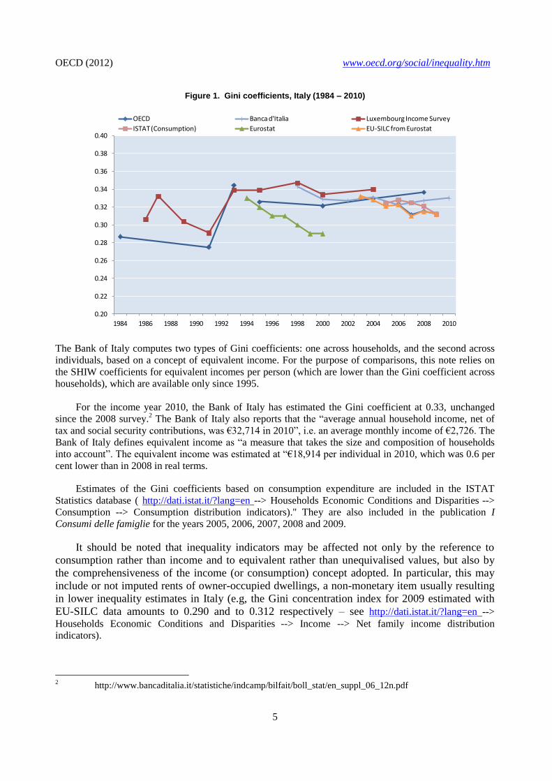
Figure 1. Gini coefficients, Italy (1984 – 2010)

The Bank of Italy computes two types of Gini coefficients: one across households, and the second across

individuals, based on a concept of equivalent income. For the purpose of comparisons, this note relies on

the SHIW coefficients for equivalent incomes per person (which are lower than the Gini coefficient across

households), which are available only since 1995.

For the income year 2010, the Bank of Italy has estimated the Gini coefficient at 0.33, unchanged

since the 2008 survey.2 The Bank of Italy also reports that the “average annual household income, net of

tax and social security contributions, was €32,714 in 2010”, i.e. an average monthly income of €2,726. The

Bank of Italy defines equivalent income as “a measure that takes the size and composition of households

into account”. The equivalent income was estimated at “€18,914 per individual in 2010, which was 0.6 per

cent lower than in 2008 in real terms.

Estimates of the Gini coefficients based on consumption expenditure are included in the ISTAT

Statistics database ( http://dati.istat.it/?lang=en --> Households Economic Conditions and Disparities -->

Consumption --> Consumption distribution indicators)." They are also included in the publication I

Consumi delle famiglie for the years 2005, 2006, 2007, 2008 and 2009.

It should be noted that inequality indicators may be affected not only by the reference to

consumption rather than income and to equivalent rather than unequivalised values, but also by

the comprehensiveness of the income (or consumption) concept adopted. In particular, this may

include or not imputed rents of owner-occupied dwellings, a non-monetary item usually resulting

in lower inequality estimates in Italy (e.g, the Gini concentration index for 2009 estimated with

EU-SILC data amounts to 0.290 and to 0.312 respectively – see http://dati.istat.it/?lang=en -->

Households Economic Conditions and Disparities --> Income --> Net family income distribution

indicators).

2 http://www.bancaditalia.it/statistiche/indcamp/bilfait/boll_stat/en_suppl_06_12n.pdf

0.20

0.22

0.24

0.26

0.28

0.30

0.32

0.34

0.36

0.38

0.40

1984 1986 1988 1990 1992 1994 1996 1998 2000 2002 2004 2006 2008 2010

OECD Banca d'Italia Luxembourg Income Survey

ISTAT (Consumption) Eurostat EU-SILC from Eurostat

OECD (2012) www.oecd.org/social/inequality.htm

6

Over the period 1984 – 2010, income inequalities remained pretty stable in Italy, with the Gini

coefficients ranging between 0.30 and 0.35, with only exception of the period 1991-1993 where

inequalities recorded a significant increase. Gini coefficients from the different databases available are all

included within this corridor. More detailed patterns in different sub-periods are provided below:

- From 1984 to 1993, OECD data can be compared with the Luxembourg Income Survey. Both

series follow the same trend, which is not surprising as both time-series are based on the Survey on

Household Income and Wealth (SHIW) conducted by the Bank of Italy. Over this decade,

inequalities remained stable except between 1991 and 1993 where Gini coefficients rose up to

0.345 according to the OECD (0.339 according to the LIS) over these two years.

- From 1995 to 2004, OECD data points can be compared with those from the Bank of Italy (Survey

on Household Income and Wealth), Eurostat and the Luxembourg Income Survey. Over this period

of time, inequalities remained pretty stable around 0.32. The Bank of Italy recorded a Gini

coefficient of 0.362 for household income and 0.329 for equivalent income in 19951.

- From 1995 to 2000, the spread between the OECD estimates and the Eurostat’s ones widened. In

2000, the spread (0.44) was the largest between the Gini coefficient computed by Eurostat (0.290)

and the one calculated by the Luxembourg Income Survey (0.334). The estimates by the OECD

and the Bank on Italy were between these two values.

- From 2006 onwards, OECD data can be compared with Bank of Italy, EU-SILC and ISTAT data.

OECD estimates for this sub-period coincide with the EU-SILC ones. The difference between the

various series narrowed over this period, which can partly be explained by the increased use of the

same source of inputs.

Overall, Figure 1. shows a growing convergence of data over time between the different datasets

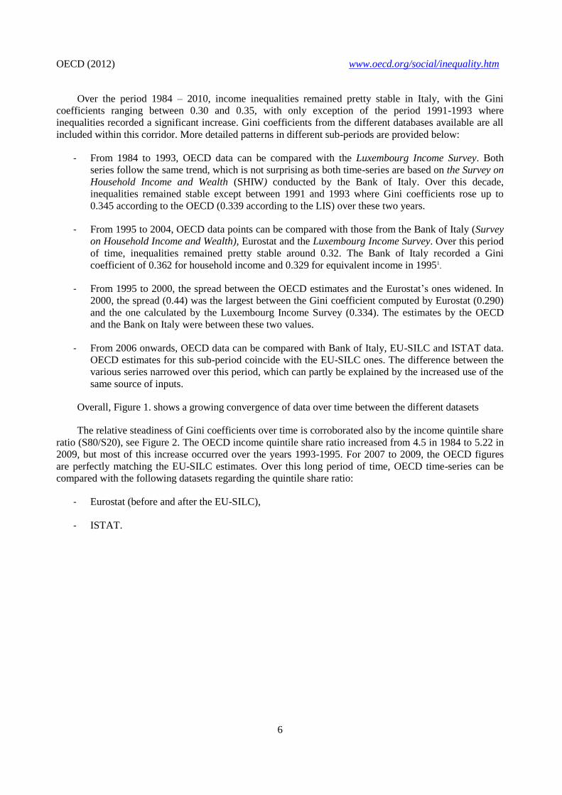
The relative steadiness of Gini coefficients over time is corroborated also by the income quintile share

ratio (S80/S20), see Figure 2. The OECD income quintile share ratio increased from 4.5 in 1984 to 5.22 in

2009, but most of this increase occurred over the years 1993-1995. For 2007 to 2009, the OECD figures

are perfectly matching the EU-SILC estimates. Over this long period of time, OECD time-series can be

compared with the following datasets regarding the quintile share ratio:

- Eurostat (before and after the EU-SILC),

- ISTAT.

OECD (2012) www.oecd.org/social/inequality.htm

7

Figure 2. S80/S20 ratio, Italy (1984 – 2010)

Between 1995 and 2000, the OECD estimates of the S80/S20 ratio slightly declines to 5.5 in 2004. In

2000, this ratio as calculated by the OECD was higher than the one recorded by Eurostat (5.5% for the

OECD vs. 4.8% for Eurostat).

Since 2003, the OECD levels of this ratio match those computed by Eurostat based on EU-SILC.

Over this period, income distribution inequality appears to have been slightly declining to 5.2% (both for

the OECD and for EU-SILC) in 2009, the latest available data.

The convergence between OECD and EU-SILC time-series regarding the income quintile share ratio

is also confirmed by ISTAT figures.

2.1.2 Time series of poverty rates

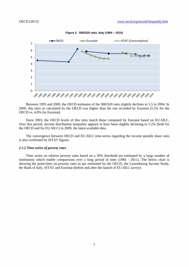
Time series on relative poverty rates based on a 50% threshold are estimated by a large number of

institutions which enable comparisons over a long period of time (1984 - 2011). The below chart is

showing the point-lines on poverty rates as per estimated by the OECD, the Luxembourg Income Study,

the Bank of Italy, ISTAT and Eurostat (before and after the launch of EU-SILC survey)

0

1

2

3

4

5

6

7OECD Eurostat ISTAT (Consumption)

OECD (2012) www.oecd.org/social/inequality.htm

8

Figure 3. Relative Poverty Rates with a 50% Threshold, Italy (1984 – 2011)

The latest available relative poverty rate was estimated by ISTAT at 11.1% in 2011 (absolute poverty

is 5.2%)3, broadly unchanged from the previous year (11.0%). According to the national statistical office,

the relative poverty threshold for a two-member household was equal to 1.011 euros per month, up from

992 euros in 2010 (without taking into consideration the variations both of consumer prices and of the

mean of consumption expenditure)4.

Since 1984, relative poverty rates have been quite stable with a few movements up to now. OECD

time-series can be compared over different sub-periods:

- From 1984 to 1995, relative poverty rates remained stable up to 1991 before increasing

significantly between 1991 and 1994, from 11.1% to 14.2%. OECD time-series and the

Luxembourg Income Survey ones perfectly match, as both time-series are based on data from

SHIW. Bank of Italy’s poverty estimates are based on the concept of equivalent income.

- From 1995 to 2006, the OECD time-series shows a decrease of poverty rates from 14.7% in

1995 to 11.8% in 2004. This decrease is also confirmed by Eurostat, whose estimate decline

from 14% in 1994 to 12.4% in 2006. Over the same period, data from Bank of Italy, ISTAT

and LIS also recorded a decline, but smaller than the OECD one.

- From 2006 onwards, the OECD time-series is pretty unchanged, from 12.5% in 2006 to

12.1% in 2009, as are the Eurostat and ISTAT time-series. In contrast, the data from the Bank

of Italy show a slight increase over the period (to a level of 14.4% in 2010).

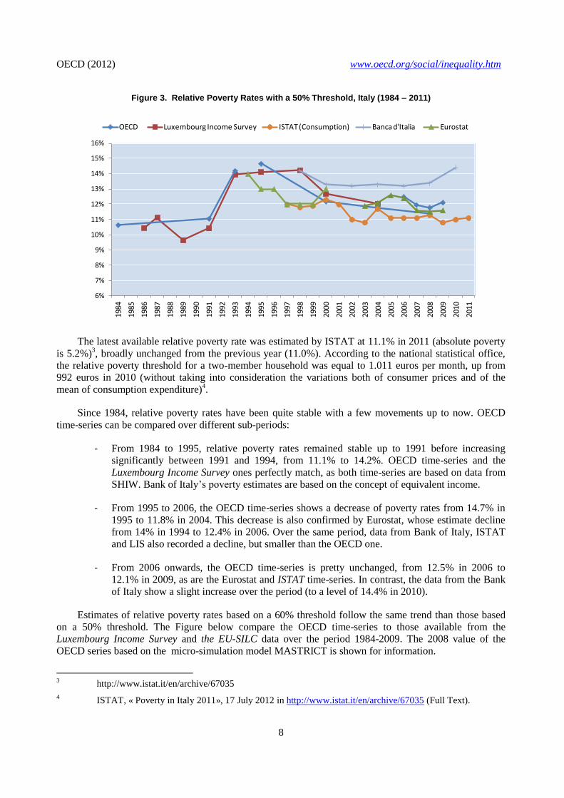
Estimates of relative poverty rates based on a 60% threshold follow the same trend than those based

on a 50% threshold. The Figure below compare the OECD time-series to those available from the

Luxembourg Income Survey and the EU-SILC data over the period 1984-2009. The 2008 value of the

OECD series based on the micro-simulation model MASTRICT is shown for information.

3 http://www.istat.it/en/archive/67035

4 ISTAT, « Poverty in Italy 2011», 17 July 2012 in http://www.istat.it/en/archive/67035 (Full Text).

6%

7%

8%

9%

10%

11%

12%

13%

14%

15%

16%

1984

1985

1986

1987

1988

1989

1990

1991

1992

1993

1994

1995

1996

1997

1998

1999

2000

2001

2002

2003

2004

2005

2006

2007

2008

2009

2010

2011

OECD Luxembourg Income Survey ISTAT (Consumption) Banca d'Italia Eurostat

OECD (2012) www.oecd.org/social/inequality.htm

9

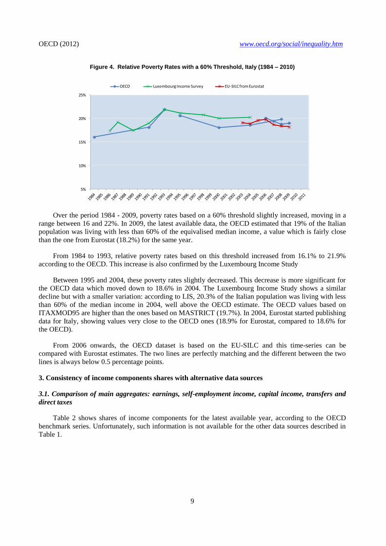
Figure 4. Relative Poverty Rates with a 60% Threshold, Italy (1984 – 2010)

Over the period 1984 - 2009, poverty rates based on a 60% threshold slightly increased, moving in a

range between 16 and 22%. In 2009, the latest available data, the OECD estimated that 19% of the Italian

population was living with less than 60% of the equivalised median income, a value which is fairly close

than the one from Eurostat (18.2%) for the same year.

From 1984 to 1993, relative poverty rates based on this threshold increased from 16.1% to 21.9%

according to the OECD. This increase is also confirmed by the Luxembourg Income Study

Between 1995 and 2004, these poverty rates slightly decreased. This decrease is more significant for

the OECD data which moved down to 18.6% in 2004. The Luxembourg Income Study shows a similar

decline but with a smaller variation: according to LIS, 20.3% of the Italian population was living with less

than 60% of the median income in 2004, well above the OECD estimate. The OECD values based on

ITAXMOD95 are higher than the ones based on MASTRICT (19.7%). In 2004, Eurostat started publishing

data for Italy, showing values very close to the OECD ones (18.9% for Eurostat, compared to 18.6% for

the OECD).

From 2006 onwards, the OECD dataset is based on the EU-SILC and this time-series can be

compared with Eurostat estimates. The two lines are perfectly matching and the different between the two

lines is always below 0.5 percentage points.

3. Consistency of income components shares with alternative data sources

3.1. Comparison of main aggregates: earnings, self-employment income, capital income, transfers and

direct taxes

Table 2 shows shares of income components for the latest available year, according to the OECD

benchmark series. Unfortunately, such information is not available for the other data sources described in

Table 1.

5%

10%

15%

20%

25%

OECD Luxembourg Income Survey EU-SILC from Eurostat

OECD (2012) www.oecd.org/social/inequality.htm

10

Table 2. Shares of income components in total disposable income, OECD reference series

Please, note the following definitions:

- EH refers to the wage and salary income of the household head, excluding employers’

contributions to social security, but including sick pay paid by governments.

- ES refers to the wage and salary income of the household spouse, excluding employers’

contributions to social security, but including sick pay paid by governments.

- EO refers to the wage and salary income from other household members, excluding employers’

contributions to social security, but including sick pay paid by governments.

Figure 5 compares trends in shares of public cash transfers in equivalised disposable income from

the OECD reference series with the share of total cash social spending in net national income, reported

from the OECD Social Expenditure database (OECD SOCX). OECD SOCX series include pensions,

incapacity, family, unemployment, social assistance. Both series show similar trends from 1999 onwards

with the exception of the slight decrease from 2005 to 2005 which is not observable in the OECD SOCX

series

Figure 5. Trends in shares of public social transfers

4. Metadata of data sources which could explain differences and inconsistencies

Definitions, methodology, data treatment

No major inconsistancies can be highlighted. The following points should be considered:

Differences between the OECD reference series and the ISTAT reported data

- As regards Gini coefficients and S80/S20 ratios, ISTAT is not publishing its methodology in

English;

OECD (2012) www.oecd.org/social/inequality.htm

11

- Even if the figures are matching pretty well, the definition of relative poverty rates are different

between the OECD and ISTAT. Indeed, poverty rates are based on median disposal incomes for

the OECD whereas these rates are based on a average consumption expenditures for ISTAT. This

term is defined as the following by the two institutions:

o The ISTAT estimate “is based on a poverty line (International standard of poverty Line-

ISPL) defining as poor a household of two components with a consumption expenditure level

lower or equal to the mean per-capita consumption expenditure (for different size households

an equivalence scale is used to take into account different needs and the

economies/diseconomies of scale that can be achieved in bigger/smaller households).

Therefore, the poverty line set the consumption expenditure level which represents the

threshold discriminating between poor and non poor households” (ISTAT Statistics Website).

The figures on relative poverty rates provided by ISTAT are labelled as “household relative

poverty incidence in percentage”.

o For the OECD, “the relative poverty threshold is expressed as a given percentage of the

median disposable income, expressed in nominal terms (current prices). Therefore, this

threshold changes over time, as the median income changes over time. Two relative poverty

thresholds are used: the first one is set at 50% of the median equivalised disposable income

of the entire population, the second one is set at 60% of that income5”.

Differences between the OECD reference series and Eurostat

- The OECD time-series has been based on EU-SILC since its implementation in Italy. Therefore,

Gini coefficients and S80/S20 ratios as published by Eurotstat are very close to the ones based on

the OECD database since 2003 (income year);

- OECD and EU-SILC data present minor differences in relative poverty rates, which are always

lower for EU-SILC than for the OECD. These differencs might be explained by the use of different

equivalence scales (the OECD reference series uses the square root of household size, whereas

Eurostat uses the OECD modified equivalence scale).

- Over 1994 to 2003, Eurostat computed income inequality and poverty indicators based on ECHP.

Despite the different sources, levels and trends were pretty similar with OECD ones.

Differences between the OECD reference series and the Luxembourg Income Survey

- For the indicators mentioned in this Quality Review, the OECD time-series and the Luxembourg

Income Survey match pretty well. This is explained by the fact that both institutions largely rely on

the Bank of Italy’s SHIW. When there are discrepancies between the OECD and the LIS before

2004, they can be explained by the interpolation of data that the OECD undertook after 2006 to

have a consistent time-series over time. For example, the Gini coefficient in 1991 as calculated by

the OECD was estimated at 0.29 before interpolation (labeled as “previous” in the OECD database)

and at 0.27 after the interpolation. The Gini coefficient recorded in the LIS for 1991 was also 0.29.

Differences between the OECD and the SHIW series from the Bank of Italy

- The OECD time-series on income inequalities and poverty rates were based on the Survey of

Household Income and Wealth from 1984 to 2009 when EU-SILC was adopted.

5 OECD Terms of References – Wave 6

OECD (2012) www.oecd.org/social/inequality.htm

12

- Gini coefficients have been always slightly higher for the bank of Italy than for the OECD. The

gap between the two time-series widened over time, to 0.012 in 2008.

- Relative poverty rates have always been slightly higher for the Bank of Italy than for the OECD

(between 1 and .2 percentage points). However, trends in the two series are pretty similar, with

both series showing broad stability.

5. Summary evaluation

Compared to some other OECD countries, long OECD time-series are available for Italy on income

inequality distribution and poverty. In addition, several national statistics exist in Italy on these indicators,

which enable a broad range of comparisons.

Over time and taking into account the different available databases, the OECD time-series match

pretty well those used in national and European reporting. Despite slight differences regarding the levels of

the different indicators, general patterns and trends are quite similar. Differences in methodology and

definitions among the sources may arise and explain the observed differences in levels for all the indicators

which are studied in this Review.

1 http://www.bancaditalia.it/statistiche/indcamp/bilfait/boll_stat/shiw98.pdf