Income Inequality and Income Segregation

Sean F. Reardon Kendra Bischoff

Stanford University

January 2010

Direct correspondence to sean f. reardon (sean.reardon@stanford.edu). An earlier version of this paper was presented at the Annual Meeting of the American Sociological Association (Boston, August 2008) and the Meeting of the International Sociological Association Research Committee on Social Stratification and Mobility (RC28) (Stanford University, August 2008). We thank participants in the University of Chicago’s Sociology Workshop for helpful feedback. We thank Steve Graham and Yosef Bodovski for programming assistance. Research for this paper was supported by the National Science Foundation (grant SES-0520400 to Reardon and a Graduate Research Fellowship to Bischoff) and the William T. Grant Foundation (Reardon).

 

 

Income Inequality and Income Segregation

Abstract

Both income inequality and income segregation in the United States grew substantially from 1970

to 2000. Using data from the 100 largest metropolitan areas, we investigate whether and how income

inequality affects patterns of income segregation along three dimensions—the spatial segregation of

poverty and affluence; race-specific patterns of income segregation; and the geographic scale of income

segregation. We find a robust relationship between income inequality and income segregation, an effect

that is larger for black families than it is for white families. In addition, income inequality affects income

segregation primarily through its effect on the large-scale spatial segregation of affluence, rather than by

affecting the spatial segregation of poverty or by altering small-scale patterns of income segregation.

Introduction

After decades of decline, income inequality in the United States has grown substantially in the

last four decades. The national Gini coefficient of household income inequality, for example, rose from

.394 in 1970 to .403, .428, and .462 in 1980, 1990, and 2000, respectively.1 At the same time, income

segregation has grown as well (Jargowsky, 1996; Mayer, 2001b; Watson, 2009; Wheeler & La Jeunesse,

2006), though the details of how and why income segregation has grown have been much less thoroughly

investigated than they have been for income inequality. Common sense and empirical evidence suggest

that these trends are linked—greater inequality in incomes implies greater inequality in the housing and

neighborhood “quality” that families or individuals can afford—but it is less clear in what specific ways

income inequality affects income segregation.

Income segregation—by which we mean the uneven geographic distribution of income groups

within a certain area—is a complex, multidimensional phenomena.2 In particular, income segregation

may be characterized by the spatial segregation of poverty (the extent to which the lowest-income

households are isolated from middle- and upper-income households) and/or the spatial segregation of

affluence (the extent to which the highest-income households are isolated from middle- and lower-income

households). In addition, income segregation may occur at different geographic scales. High- and low-

income households may be spatially far from one another or may be in economically homogeneous

neighborhoods that are spatially near one another (Reardon, et al., 2008). And given the strong

correlation between income and race in the U.S., income segregation is often empirically entangled with

racial segregation, implying the necessity of examining income segregation separately by race as well as

for the population as a whole.

Income segregation—and its causes and trends—is of interest to sociologists because income

segregation may lead to inequality in social outcomes. Income segregation implies, by definition, that

1 http://www.census.gov/hhes/www/income/histinc/p60no231_tablea3.pdf (retrieved 2 September, 2009). 2 Throughout this paper, we focus on the spatial evenness dimension of income segregation (Massey & Denton, 1988; Reardon & O'Sullivan, 2004) because this dimension maps most closely onto our theoretical model of how income inequality is related to residential household income distribution patterns. Below we discuss the relationship of this dimension to patterns of concentration and exposure.

1

lower-income households will live, on average, in neighborhoods with lower average incomes than do

higher-income households. If the average income of one’s neighbors (and/or its correlates) indirectly

affects one’s own social, economic, or physical outcomes (and a large range of sociological theories

predict such contextual effects; see, for example, Jencks & Mayer, 1990; Leventhal & Brooks-Gunn,

2000; Morenoff, 2003; Sampson, Raudenbush, & Earls, 1997; Sampson, Raudenbush, & Sharkey, 2008),

then income segregation will lead to more unequal outcomes between low- and high-income households

than their differences in income alone would predict. In a highly segregated region, then, higher-income

households may be advantaged relative to lower-income households not only by the difference in their

own incomes, but by the differences in their respective neighbors’ incomes.

Given the potential consequences of income segregation on social, political, and health-related

outcomes, it is important to understand how it is produced. In this paper, we seek to understand whether

and how income inequality leads to income segregation. More specifically, we seek to understand if and

how variation in income inequality—including variation in inequality among metropolitan areas, between

racial groups, and over time—has shaped patterns of income segregation in the years 1970-2000. Despite

the importance of understanding the connection between income inequality and income segregation, few

studies have addressed these questions (for exceptions, see Mayer, 2000; Watson, 2009). Moreover,

while these studies find that increasing income inequality leads to (or is at least correlated with)

increasing income segregation, they do not investigate the ways in which income inequality is linked to

income segregation in depth. As a result, these studies provide little or no information about income

inequality’s effects on the segregation of poverty and/or affluence, about racial differences in income

segregation, or about how income inequality impacts the spatial scale of income segregation.

The research presented here investigates these issues. First, we describe a set of trends in average

metropolitan area income segregation from 1970-2000, including overall trends, trends among white and

black families separately, trends in the segregation of poverty and affluence, and trends in the geographic

scale of segregation. We use a newly developed measure of rank-order income segregation that avoids

the confounding of changes in the income distribution with changes in income segregation. Second, we

2

estimate the effect of metropolitan area income inequality on overall metropolitan area income

segregation during this time period. Third, we investigate in more detail how income inequality affects

the geographic segregation of poverty and affluence, the extent to which it affects income segregation

among white and black families differently, and the ways that it impacts the geographic scale of income

segregation.

Background

Recent Growth in Income Inequality in the United States

20th century United States income inequality is characterized by a “U-shaped” trend (Nielsen &

Alderson, 1997; Ryscavage, 1999). Income inequality was high in the first half of the century, reaching a

peak in the late 1920s, when the top 10% of earners in the U.S. received 46% of all income and the top

1% of earners received nearly 20% of all income (Piketty & Saez, 2003). However, the Great Depression

and World War II greatly depleted the share of income held by the highest earners and thus reduced

income inequality substantially. By the end of World War II, the share of income received by the top 1%

of earners was only 11% and by 1970, this figure was below 8%, a 60% decline from its high in 1928. In

the 1970s and 1980s, income inequality began to rise again. By 2006, the share of income held by the top

decile was 45% and the share held by the top 1% of earners was 18%, approaching inequality levels

similar to the pre-World War II highs (Burkhauser, Feng, Jenkins, & Larrimore, 2009; Piketty & Saez,

2003, 2008).

The growth in income inequality in the past four decades has been driven largely by the growth of

“upper-tail inequality”—dispersion in the relative incomes of those in the upper half of the income

distribution—rather than by growth in “lower-tail inequality” (Autor, Katz, & Kearney, 2006, 2008;

Piketty & Saez, 2003). This pattern is illustrated in Figure 1, which shows the changes in the household

Gini index (a standard summary measure of income inequality), the 90/50 household income ratio (the

ratio of the income of the household at the 90th percentile of the income distribution to that of the

household at the 50th percentile), and the 50/10 household income ratio. The 90/50 ratio was 30% larger

3

in 2007 than it was in 1967, while the 50/10 ratio was actually 6-7% smaller. This implies that the lower

tail of the income distribution was compressed slightly (particularly in the early 1970s) while the upper

tail was stretched.3 Moreover, the growth in the household Gini index over the period very closely tracks

the growth in the 90/50 ratio, indicating that the trend in the Gini index was driven largely—if not

entirely—by growth in upper-tail inequality. Picketty and Saez (2003) argue that the notoriously sharp

increase in CEO pay evident in recent decades is indicative of a general shift from an elite rentier class in

the beginning of the 20th century to an elite “working rich” class today, leading to the exceptional rise in

inequality in the upper tail of the distribution.4 As we discuss below, this pattern of growth in income

inequality has important implications for the effects of income inequality on income segregation.

Figure 1 here

Dimensions of Income Segregation

Income segregation—the uneven sorting of households or families among neighborhoods by

income—is relatively ubiquitous in the U.S. 5 Anyone who has rented an apartment or bought a house

understands that housing costs more in some neighborhoods than it does in others. Except for those few 3 The trend in the 50/10 ratio we report here differs slightly than that reported by Autor, Katz, and Kearney, (2006, 2008), who find that the 50/10 ratio grew in the 1970s and early 1980s before flattening in the late l980s and 1990s. The discrepancy may arise from the fact that they describe trends in individual-level male and female wage inequality using CPS data while Figure 1 reports household income inequality. Regardless, in both cases, the dominant factor in producing income inequality growth in recent decades has been the growth of what they term “upper-tail inequality.” 4 A large body of research investigates the causes of the growth in income inequality in the United States since the 1970s. Economists have focused on declining labor union membership, the declining real value of the minimum wage, and the ways in which technological changes have differentially affected the productivity of workers (Card & DiNardo, 2002; Card, Lemieux, & Riddell, 2004; DiPrete, 2007; D. S. Lee, 1999; Levy & Murnane, 1992). Sociologists have investigated factors relating to changes in family structure, marital homogamy, and female labor force participation (Gottschalk & Danziger, 2005; Schwartz & Mare, 2005; Western, Bloome, & Percheski, 2008). In the interest of space, we do not review this literature here. 5 Throughout this paper we are most interested theoretically in household income segregation (rather than family or individual income segregation), because households are primary residential units and so are most relevant to a discussion of segregation. Nonetheless, because of data limitations (e.g., the Census reports family income by race but not household income by race in some years), we use family income in much of our analysis. Although family income is generally higher on average than household income because many households only contain one person, the trends in inequality for families and households are very highly correlated (for trend in family Gini index, see http://www.census.gov/hhes/www/income/histinc/f04.html; for trend in household Gini index, see http://www.census.gov/hhes/www/income/histinc/p60no231_tablea3.pdf) (the correlation is 0.997, according to Moller, Alderson, & Nielsen, 2009, footnote 13). Likewise, the shape of the trends in metropolitan area family and household income segregation are similar as well (Watson, 2009; Wheeler & La Jeunesse, 2008).

4

with liquid wealth, income is a primary determinant of neighborhood affordability. Moreover, housing

prices are tightly linked to the cost of nearby housing. Realtors, appraisers, and homebuyers use recent

sale prices of comparable neighborhood real estate to gauge appropriate sale prices for nearby properties,

which leads to positive feedback in local housing markets. And because mortgage loans are tied to

income (the last few years notwithstanding), homebuyers’ neighborhood options are constrained by their

incomes. In principle, these mechanisms operate to place a (somewhat permeable) floor on the incomes

of individuals who can afford to live in a given neighborhood, leading to a certain degree of residential

sorting by income.

Income segregation has multiple dimensions. First, neighborhood sorting of families or

households by income may produce the segregation of affluence and/or the segregation of poverty (by

“segregation of affluence,” we mean the uneven distribution of high-income and non-high-income

households among neighborhoods, and by “segregation of poverty,” we likewise mean the uneven

distribution of low- and non-low-income households among neighborhoods).6 Consider a stylized

population made up of three types of families—high-, middle-, and low-income—who are distributed

among three neighborhoods (See Table 1). Under scenario I, the low-income families all live in a single

neighborhood, with no middle- or high-income neighbors, while the middle-and high-income families are

evenly distributed between the other two neighborhoods—a situation where the segregation of poverty is

greater than the segregation of affluence (high-income families have some non-high-income neighbors,

but low-income families have only low-income neighbors). Under scenario II, the situation is reversed—

the segregation of affluence is greater than the segregation of poverty. And finally, in scenario III, the

segregation of both poverty and affluence are very high. 6 Note that we mean to distinguish the terms “segregation of poverty” and “segregation of affluence” from the more commonly-used terms “concentrated poverty” and “concentrated affluence.” The latter terms are often used to describe the income composition of individual neighborhoods (e.g., neighborhoods with poverty rates above 40% are sometimes described as being characterized by “concentrated poverty.”), rather than patterns of the distribution of income across multiple neighborhoods in a city or region. In addition, we intend to identify “segregation of poverty” and “segregation of affluence” as aspects of the spatial evenness dimension of segregation, rather than as descriptions of the concentration dimension (Massey & Denton, 1988; Reardon & O'Sullivan, 2004). We can have high levels of “segregation of poverty” without the spatial concentration of poor households within one area of a region (for example, if low-income families live in many neighborhoods scattered throughout a metropolitan area, but not in the same census tracts as higher-income families).

5

Table 1 here

A second important dimension of income segregation is its relationship to patterns of racial

segregation. Given the correlation of race and income in the U.S. and the high levels of racial segregation

in many metropolitan areas, racial segregation alone could produce a certain degree of income

segregation, even if there were no within-race income segregation at all. Moreover, the factors that affect

income segregation and that link income inequality to income segregation may differ importantly across

race/ethnic groups. Housing discrimination and residents’ preferences for same- or different-race

neighbors, for example, may also affect residential sorting. Until relatively recently, black families’

neighborhood options were severely constrained by various discriminatory housing practices (steering by

realtors, redlining by banks, rental discrimination, etc.), and even now these processes have not been

entirely eradicated (Ross & Turner, 2005; South & Crowder, 1998; Turner & Ross, 2005; Turner, Ross,

Galster, & Yinger, 2002; Yinger, 1995). Such practices meant that black and white families with

identical incomes and assets, for example, had a very different set of residential options. This also likely

meant that, historically, income inequality was not as tightly linked to income segregation for black

families as it was for white families.

A third dimension of income segregation is its geographic scale (Reardon, et al., 2009; Reardon,

et al., 2008). This refers to the extent to which the neighborhood sorting of households by income results

from large-scale patterns of residential sorting (as would be the case if all high-income families live in the

suburbs, and all low-income families live in the city) or from small-scale patterns of residential sorting (as

would be the case if high- and low-income residents were distributed in a checkerboard pattern

throughout a metropolis, with homogenously wealthy neighborhoods adjacent to homogeneously poor

neighborhoods throughout the area). The extent to which income segregation is characterized by large or

small geographic scales may have implications for the consequences of income segregation (a point

indirectly supported by the results of Firebaugh & Schroeder, 2007). Reardon and colleagues argue, for

example, that micro-scale residential segregation patterns are likely to affect pedestrian contact patterns

and may be more consequential for children and the elderly, who are often more geographically

6

constrained than young and middle-aged adults. Conversely, they argue, macro-scale segregation patterns

may be more likely to affect the spatial distribution of economic, institutional, and political resources

(Reardon, et al., 2009; Reardon, et al., 2008).

Patterns and Trends in Income Segregation

Most prior research on income segregation has focused on measuring overall income segregation,

and has attended little to either the geographic scale of income segregation or the extent to which it is

characterized by the segregation of poverty and/or affluence. Research on the trends in overall household

or family income segregation generally indicate that metropolitan area income segregation grew, on

average, from 1970 to 2000, though studies differ on the details of the timing and magnitude of the

increase because of differences in the measures of income segregation used and the sample of

metropolitan areas included (see Jargowsky, 1996, 2003; Massey & Fischer, 2003; Mayer, 2001b;

Watson, 2009; Wheeler & La Jeunesse, 2006). In particular, income segregation appears to have grown

most sharply in the 1980s. By many measures, income segregation, and particularly the segregation of

poverty, declined in the 1990s (Jargowsky, 2003; Massey & Fischer, 2003; Yang & Jargowsky, 2006). In

addition, studies that examine trends in income segregation by race generally find that income segregation

among black families or households grew faster than it did among white families or households,

particularly during the 1970s and 1980s (Jargowsky, 1996; Massey & Fischer, 2003; Watson, 2009; Yang

& Jargowsky, 2006). Later in this paper we discuss the shortcomings of many of the measures of income

segregation used in prior literature and present new evidence of trends in metropolitan area income

segregation. We use a new measure of income segregation that addresses these shortcomings.

Potential Consequences of Income Segregation

There are many mechanisms through which income segregation might affect individual

outcomes. The quality of public goods and local social institutions are affected by a jurisdiction’s tax base

and by the involvement of the community in the maintenance and investment of these public resources. If

7

high-income households cluster together within a small number of neighborhoods or municipalities, they

may be able to collectively better their own outcomes by pooling their extensive financial and social

capital to generate resources of which only they can take advantage. Such income segregation may be

self-reinforcing: low-income communities are often unable to generate enough social and human capital

to overcome the strong incentive for wealthy communities to isolate themselves, because in

homogenously high-income communities residents may be able to capitalize on their ability to provide

high-quality public services at the lowest cost. Higher-income neighborhoods, therefore, may have more

green space, better-funded schools, better social services, or more of any number of other amenities that

affect quality of life. In addition, high- and low-income neighborhoods may differ in their social

processes, norms, and social environments (Sampson, Morenoff, & Earls, 1999; Sampson, et al., 1997).

Conversely, if high-income households are not clustered together, then they may help to fund social

services and institutions that serve lower-income populations. Thus, the ability of high-income

households to self-segregate affects the welfare of poor people and the neighborhoods in which they

reside. Not only does this resource problem affect residents’ current quality of life and opportunities, but

it can also bridge generations—the income distribution in a community may affect the intergenerational

transfer of occupational status through investment in locally financed institutions that serve children, such

as schools (Durlauf, 1996).

Nonetheless, relatively little prior research has directly assessed the impacts of income

segregation on individual outcomes. Several studies show that income segregation within states or

metropolitan areas is associated with greater inequality in educational attainment between poor and non-

poor individuals (Mayer, 2000; Quillian, 2007). Likewise, Mayer and Sarin (2005) show that greater

state-level income segregation is associated with higher rates of infant mortality. A related body of

research finds that metropolitan area racial segregation leads to greater racial inequality in labor market,

educational, and health outcomes (Ananat, 2007; Cutler & Glaeser, 1997; Ellen, 2000; Osypuk &

Acevedo-Garcia, 2008). Because racial segregation implies some level of income segregation (given the

relatively large racial differences in income), and because income segregation is one plausible mechanism

8

through which racial segregation may lead to racial inequality, the research showing that racial

segregation increases racial disparities is consistent with the hypothesis that income segregation may lead

to inequality of outcomes. In addition to the relatively small body of research directly investigating the

effects of income segregation, a large body of recent research has attempted to investigate one potential

mechanism through which segregation may affect individuals—the effect of living in a neighborhood

with a high poverty rate. The empirical evidence for such ‘neighborhood effects’, however, remains both

mixed and contested (see, for example, Clampet-Lundquist & Massey, 2008; Jencks & Mayer, 1990;

Katz, Kling, & Liebman, 2007; Leventhal & Brooks-Gunn, 2000; Ludwig, et al., 2008; Rosenbaum &

Popkin, 1991; Sampson, 2008; Sampson, et al., 1997; Sampson, et al., 2008; Waitzman & Smith, 1998a,

1998b). In sum, while theoretical arguments suggest that income segregation likely produces inequality

in social outcomes, empirical research has yet to conclusively demonstrate this or to elucidate its

mechanisms.

The Relationship between Income Inequality and Income Segregation

Processes Linking Income Inequality to Income Segregation

Despite the need for more and better research on the effects of income segregation, this paper

focuses on an equally important topic—the causes of income segregation. Specifically, we investigate

one potential cause—income inequality. Certainly income inequality is a necessary condition for income

segregation. By definition, if there were no income inequality, there could be no income segregation

because all individuals would have the same income and thus all neighborhoods would have the same

income distribution. Nonetheless, income inequality is not alone sufficient to create income segregation.

Rather, income segregation also requires the presence of income-correlated residential preferences, an

income-based housing market, and/or housing policies that link income to residential location.

Three kinds of income-correlated residential preferences may lead to income segregation in the

presence of income inequality: preferences regarding the socioeconomic characteristics of one’s

neighbors, preferences regarding characteristics of one’s neighbors that are correlated with their income,

9

and preferences regarding local public goods. If some or all households have preferences regarding the

income level, educational attainment, or occupational status of their neighbors (that is, if at least some

households prefer higher-income neighbors to lower-income neighbors), then households with similar

incomes will be more likely to be neighbors than is expected by chance. Likewise, residential preferences

based on neighborhood characteristics that are correlated with income may also produce income

segregation. One obvious example is race. If households select neighborhoods based on the racial

composition of that neighborhood and household income is correlated with race, then this would also

produce income segregation, even in the absence of income-specific preferences.

Preferences for public goods refer to the value households place on amenities that can be

collectively purchased (e.g., public school quality, public parks, police services). Households that value

such public goods will have incentives to live in communities with neighbors who both share these

preferences and have high enough incomes to contribute to their collective purchase (through property

taxes, for example). This can be seen as a manifestation of the Tiebout model of residential sorting, in

which residents choose to live in municipalities that most closely match their ideal set of government

services with their ability-to-pay (Tiebout, 1956). The Tiebout model predicts income segregation

because households with similar preferences and ability-to-pay tend to form homogeneous communities.

Differences among communities in public goods, income-related demographic characteristics, and in

other social and cultural amenities may also lead to the development of neighborhood status hierarchies,

or what one might call “neighborhood brands.” The differentiation of communities along a status

dimension in turn raises demand for those neighborhoods with the most desirable brands (and lowers

demand for those with the least desirable brands). Thus, income differences may lead to the development

of a rough status hierarchy among residential locations; this status hierarchy in turn may perpetuate

income segregation by shaping household preferences.

Even in the presence of sizeable income inequality, however, the income-correlated preferences

outlined above may be insufficient to produce income segregation. Income segregation requires as well

the existence of a housing market based on residents’ ability-to-pay or housing policies that sort

10

households by income. For example, housing policies that constrain residential options for low-income

households to public housing developments may directly affect the segregation of poverty by virtue of the

spatial density and distribution of those options. More generally, income segregation results from a

residential allocation or sorting process, which, in principle, is constrained by housing policy. Under a

housing policy that allows sorting on the basis of preferences and ability-to-pay, residential segregation

will likely be highly sensitive to changes in income inequality and income-related residential preferences

because, in such a society, higher-income households will be able to outbid lower-income households for

access to preferred neighborhoods. In addition, when higher-income households have greater influence

than lower-income households over local political processes, they may have the capacity to create

housing policies that perpetuate segregation by income, such as zoning laws that prohibit multifamily

housing or require minimum lot sizes to build new structures.

Income Inequality and the Segregation of Poverty and Affluence

The above arguments suggest that, given the nature of the housing market, income inequality and

income segregation are linked. Nonetheless, it is not clear if or how changes in income inequality might

affect different aspects of income segregation, including the segregation of poverty and affluence. In

order to build intuition about how income inequality may relate to income segregation, it is useful to

consider how differences in income inequality are related to differences in income distributions. Figure 2

provides a stylized representation of two income distributions with equal aggregate incomes but that

differ in their level of inequality. The solid lines describe the income distribution under a relatively low

level of inequality (corresponding to a Gini index of 0.34), while the dashed lines describe the income

distribution under a relatively high level of inequality (corresponding to a Gini index of 0.40).7

7 The average level of income inequality across the 100 largest metropolitan areas in the years 1970-2000, as measured by the Gini index was 0.37, with a standard deviation of 0.03 (see Table 2 below for detail), so Gini indices of 0.34 and 0.40 correspond to metropolitan areas one standard deviation above and below the mean level of inequality in the period 1970-2000. Likewise, the average metropolitan area saw an increase in the Gini index from 0.35 to 0.40 from 1970 to 2000, so these distributions also correspond roughly to the magnitude of the average change over this period.

11

Moreover, the stylized income distributions depicted here differ only in the level of “upper-tail

inequality”—the 50/10 income ratio is identical in both cases, but the 90/50 income ratio is 35% larger in

the high-inequality case than in the low inequality case.8 Note that the income distributions described in

Figure 2 are not based on actual data. Rather they are stylized distributions that exemplify typical

differences in income distributions—an exercise that highlights how the type and magnitude of inequality

relates to important features of income distributions.

Figure 2 here

The left-hand panel of Figure 2 shows that the income distribution is more spread out at the high

end under conditions of greater inequality. There is greater variation in income among high earners in the

higher-inequality distribution than in the lower-inequality distribution. At the low end of the income

distribution, however, increasing inequality actually compresses the income distribution, a result of the

fact that income must be non-negative (at least in our stylized figures here).9

The difference in the effect of income inequality at the high and low ends of the income

distributions is evident in the middle panel of Figure 2. For example, it is instructive to compare the

incomes of households at the 20th and 30th percentiles in each scenario. In the lower-inequality

distribution (solid line), the household at the 20th percentile has an income of $33,500 and the household

at the 30th percentile has an income of $43,000, a difference of $9,500 and a ratio of 1.28. In the higher-

inequality distribution (dashed line), the 20th and 30th percentile households have incomes of $29,000 and

$37,000, respectively, a difference of $8,000 and a ratio of 1.28. That is, under high inequality, low-to-

moderate income households of a given distance apart in income ranks have incomes that are actually

closer together (and equally far apart if comparing incomes using ratios) than under low inequality. This

implies that increases in income inequality of the type depicted here (that is, increases in inequality that

leave the 50/10 ratio unchanged) will not increase, and may actually decrease income segregation among

8 Because most of the change in income inequality from 1970 to 2000 was the result of changes in upper-tail inequality, we are particularly interested in investigating the effect of such changes on segregation patterns. 9 While income can be negative, the number of households reporting negative income is generally quite small and has little effect on the income distribution.

12

low-income households (segregation of poverty). This is because increasing inequality (somewhat

paradoxically) makes the incomes of low-income households more similar to one another.

The opposite is true at the high end of the income distribution. Comparing the incomes of the

70th and 80th percentile households under both the higher- and lower-inequality distributions, it is apparent

that an increase in income inequality increases the difference in incomes between these households. In

the lower-inequality distribution, the household at the 70th percentile has an income of $88,000 and the

household at the 80th percentile has an income of $106,000, a difference of $18,000, and a ratio of 1.20.

In the higher-income distribution, the 70th and 80th percentile households have incomes of $83,000 and

$109,000, respectively, a difference of $26,000 and a ratio of 1.31. That is, an increase in upper-tail

income inequality increases the difference in incomes between two moderate-to-high income households

at given percentiles of the income distribution, making it less likely that they can afford to live in the

same neighborhood. This implies that differences in income inequality that are due to differences in

upper-tail inequality—as has been the case with changes in income inequality from 1970-2000—should

lead to greater segregation of affluence but not necessarily to greater segregation of poverty.

Racial Differences in the Effects of Income Inequality

As we suggested above, income inequality may affect income segregation differently among

black and white households because of the variation in housing markets available to each group. Racial

discrimination in the housing market has meant that, historically at least, minority households

(particularly black households) have had fewer residential options than white households with similar

income and wealth. Even if black households had the same preferences and the same level of income

inequality as white households, the racially discriminatory aspects of the housing market likely led to

lower levels of income segregation among black households than among white households. This is

because the segregation of black households compelled higher- and lower-income black households to

live close to one another.

13

The black middle class grew rapidly from 1940 to 1990,10 resulting in rising income inequality

among black households (Farley & Frey, 1994; Son, Model, & Fisher, 1989). Until the passage of the

Fair Housing Act in 1968 and the Home Mortgage Disclosure Act in 1975, however, discriminatory

housing practices severely limited the residential mobility of middle-class black families (Farley & Frey,

1994). As a result, prior to 1970, income inequality among blacks was probably less tightly linked to

income segregation than it was for whites. In the period from 1970-2000, however, the housing options

available to middle-class blacks greatly expanded (though some housing discrimination persisted through

this period; see Farley & Frey, 1994; Ross & Turner, 2005; Yinger, 1995), likely tightening the link

between inequality and segregation among blacks over this period.

Empirical Predictions

The above arguments suggest several testable hypotheses. First, because the U.S. housing market

is largely based on ability-to-pay, we predict that income inequality will be positively correlated with

income segregation and that changes in income inequality with be positively associated with changes in

income segregation. Second, because most of the change in income inequality has been the result of

growth in upper-tail inequality, we predict that changes in income inequality will affect the segregation of

affluence to a greater degree than it affects the segregation of poverty. Third, we predict that income

inequality will have a stronger relationship with income segregation among black families than among

white families during the period 1970-2000, when housing market constraints were substantially reduced

for black households. Finally, although there is no existing research on the geographic scale of income

segregation, we expect that income inequality leads to income segregation primarily by increasing the

spatial distance between high- and low-income households (due to suburbanization of middle- and upper-

income households, for example). Thus, we predict that income inequality will have a stronger

relationship with macro-scale segregation patterns than with micro-scale segregation patterns.

10 Farley and Frey (1994) define middle class as having an income that is twice the poverty line. By this definition, just 1% of black households in 1940 were middle class, compared to 39% in 1970 and 47% in 1990.

14

There is little prior research regarding most of these hypotheses. Several existing studies

demonstrate a positive association between income inequality and income segregation. Mayer (2001b)

shows that the well-documented increase in income inequality from 1970-1990 resulted in an increase in

segregation between census tracts within states—although the income variance within census tracts

remained stable, the income variance between tracts grew, indicating an increase in between-tract income

segregation. Wheeler and La Jeunesse (2008) largely corroborate these findings using metropolitan areas,

rather than states, as the unit of analysis. They find that the average level of income segregation

(measured as the between-block group share of income inequality) within metropolitan areas grew

sharply in the 1980s and declined slightly in the 1990s, a pattern that is only partly consistent with the

trend in steadily rising income inequality over the same period. Because their analysis is based on a

simple comparison of trends, however, it indicates little about the causal relationship between income

inequality and segregation.

A third recent study uses metropolitan area fixed-effects regression models to estimate the causal

effect of metropolitan area income inequality on income segregation, demonstrating that income

inequality has a strong effect on income segregation (Watson, 2009). Specifically, Watson finds that a

one standard deviation rise in income inequality leads to a 0.4-0.9 standard deviation rise in income

segregation. Moreover, Watson briefly investigates several additional aspects of the relationship between

income inequality and income segregation. First, she finds that income inequality leads to increases in the

segregation of both poverty and affluence (though the effect is slightly larger on the segregation of

affluence). Second, she finds that income inequality has a weaker effect on income segregation among

black families than in the population as a whole (contrary to our hypothesis above). Finally, her results

suggest no effect of income inequality on suburbanization rates from 1970-2000, implying, perhaps, that

income inequality does not affect the geographic scale of income segregation (though Watson notes that

data limitations render these results merely “suggestive”). Nonetheless, while each of these three

analyses provides some evidence regarding our hypotheses, they each rely on segregation measures that

are not ideal. As we describe below, her preferred measure of segregation, the Centile Gap Index, does

15

not allow clear comparisons across metro areas and years and it cannot be used to measure geographic

scale. In our analyses below, we use a more appropriate measure of income segregation that allows us to

more directly estimate the effects of inequality on the segregation of affluence and poverty and on the

geographic scale of segregation.

Data and Methods

Measuring Income Segregation

To analyze income segregation it is necessary to first measure income segregation. While there is

a rich literature discussing measures of segregation among unordered categorical groups, such as race or

gender (see, for example, Duncan & Duncan, 1955; James & Taeuber, 1985; Reardon & Firebaugh, 2002;

Reardon & O'Sullivan, 2004; Taeuber & Taeuber, 1965),11 methods of measuring income segregation are

much less well developed. Unlike race or gender, income is measured on a continuous (or at least an

ordinal) scale, so measures of segregation that are appropriate for unordered categorical groups are not

appropriate for measuring income segregation. We provide here a brief review of existing approaches to

measuring income segregation and then describe the measure we will rely on, the rank-order information

theory index (Reardon, Firebaugh, O'Sullivan, & Matthews, 2006).

Much of the small body of existing literature on income segregation in sociology has measured

income segregation by using established measures of racial segregation, such as the dissimilarity index,

applied to a small set of crude income categories (poor vs. non-poor, or upper, middle, and lower

income). Examples of this approach are found in the literature in sociology (Fong & Shibuya, 2000;

Massey, 1996; Massey & Eggers, 1993; Massey & Fischer, 2003), urban planning (Coulton, Chow,

Wang, & Su, 1996; Pendall & Carruthers, 2003), economics (Jenkins, Micklewright, & Schnepf, 2006),

and public health (Waitzman & Smith, 1998b). There are a number of serious deficiencies with this

technique, including the substantial loss of information that results from treating income as categorical

11 There is also a literature in geography and economics on the measurement of categorical segregation (see, for example, Echenique & Fryer, 2005; Mora & Ruiz-Castillo, 2003; Wong, 1993, 2002).

16

and the arbitrary nature of selecting a small number of cut points to categorize the data. Even if the exact

income of families is unknown, the 16 income categories reported in the 2000 U.S. Census, for example,

contain far more information than 2 or even 4 categories. Moreover, the income categories (as well as the

meaning of a given dollar amount of income) change over time, so that categories defined in one

decennial Census cannot be replicated in another.

A second approach to measuring income segregation defines segregation as a ratio of the

between-neighborhood variation in mean income to the total population variation in income. Income

segregation measures derived from this approach have used a number of different measures of income

variation, including the variance of incomes (Davidoff, 2005; Wheeler, 2006; Wheeler & La Jeunesse,

2006), the standard deviation of incomes (Jargowsky, 1996, 1997), the variance of logged incomes

(Ioannides, 2004), the coefficient of variation of incomes (Hardman & Ioannides, 2004), and

Bourguignon’s income inequality index (Ioannides & Seslen, 2002). Similarly, the Centile Gap Index

(CGI) measures segregation as one minus the ratio of within-neighborhood variation in income percentile

ranks to the overall variation in percentile ranks (Watson, 2006, 2009). Most well-known in sociology is

Jargowsky’s (1996, 1997) Neighborhood Sorting Index (NSI), which is defined as the square root of the

ratio of the between-unit income variance to the total income variance.

Although the NSI and measures like it improve upon categorical measures of income segregation

because they do not rely on arbitrary and changing dichotomizations of income distributions, they lack a

key feature that is necessary for our purposes in this paper. In order to distinguish income segregation

(the sorting of households by income among census tracts, independent of the income distribution) from

income inequality (the uneven distribution of income among families), a measure of income segregation

is required that is independent of income inequality. One way to achieve this is to use an income

segregation measure that relies only on information about the rank-ordering of incomes among families,

rather than information about actual dollar income amounts. A rank-order income segregation measure

will be, by definition, invariant under any changes in income that leave families’ residential location and

income rank unchanged, regardless of how income inequality changes. Unfortunately, the Neighborhood

17

Sorting Index (NSI) (Jargowsky, 1996) does not satisfy this property, and so may confound changes in

income inequality with changes in residential sorting by income, and may confound differences in income

distributions across time, place, and groups with differences in segregation (Neckerman & Torche, 2007).

More suitable for our purposes is the rank-order information theory index (HR) (Reardon, et al., 2006),

which measures the ratio of within-unit (tract) income rank variation to overall (metropolitan area)

income rank variation.12

The Rank-Order Information Theory Index

Reardon and colleagues (2006) describe the rank-order information theory index in detail; we

summarize its key features here. First, let denote income percentile ranks (scaled to range from 0 to 1)

in a given income distribution (that is , where measures income and is the cumulative

income density function). Now, for any given value of , we can dichotomize the income distribution at

and compute the residential (pairwise) segregation between those with income ranks less than and

those with income ranks greater than or equal to . Let denote the value of the traditional

information theory index (James & Taeuber, 1985; Theil, 1972; Theil & Finezza, 1971; Zoloth, 1976) of

segregation computed between the two groups so defined. Likewise, let denote the entropy of the

population when divided into these two groups (Pielou, 1977; Theil, 1972; Theil & Finezza, 1971). That

is,

log1

1 log1

1

(1)

and

12 Reardon et al (2006) review a number of other measures of income segregation proposed in the literature, concluding that the rank-order information theory measure better isolates the sorting/unevenness dimension of income segregation than other measures, and ensures comparability over time and place, a feature most other measures lack. The Centile Gap Index (CGI) (Watson, 2006, 2009) shares many desirable features with HR, but lacks several important features: it does not accommodate spatial information; it does not allow straightforward examination of the segregation of poverty and affluence; and it is insensitive to certain types of sorting among neighborhoods. These shortcomings render it less preferable than HR.

18

1 ,

(2)

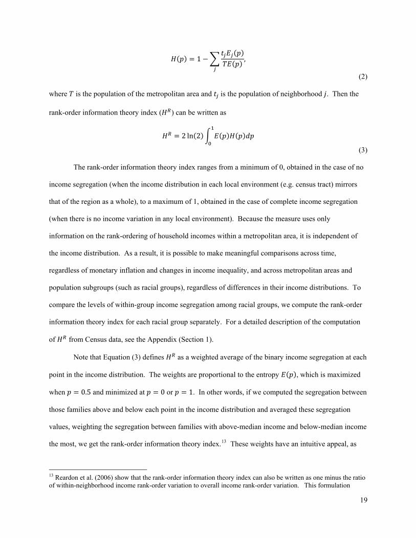
where is the population of the metropolitan area and is the population of neighborhood . Then the

rank-order information theory index ( ) can be written as

2 ln 2

(3)

The rank-order information theory index ranges from a minimum of 0, obtained in the case of no

income segregation (when the income distribution in each local environment (e.g. census tract) mirrors

that of the region as a whole), to a maximum of 1, obtained in the case of complete income segregation

(when there is no income variation in any local environment). Because the measure uses only

information on the rank-ordering of household incomes within a metropolitan area, it is independent of

the income distribution. As a result, it is possible to make meaningful comparisons across time,

regardless of monetary inflation and changes in income inequality, and across metropolitan areas and

population subgroups (such as racial groups), regardless of differences in their income distributions. To

compare the levels of within-group income segregation among racial groups, we compute the rank-order

information theory index for each racial group separately. For a detailed description of the computation

of from Census data, see the Appendix (Section 1).

Note that Equation (3) defines as a weighted average of the binary income segregation at each

point in the income distribution. The weights are proportional to the entropy , which is maximized

when 0.5 and minimized at 0 or 1. In other words, if we computed the segregation between

those families above and below each point in the income distribution and averaged these segregation

values, weighting the segregation between families with above-median income and below-median income

the most, we get the rank-order information theory index.13 These weights have an intuitive appeal, as

13 Reardon et al. (2006) show that the rank-order information theory index can also be written as one minus the ratio of within-neighborhood income rank-order variation to overall income rank-order variation. This formulation

19

they imply the extent of segregation between those above and below the median is more informative

about overall residential sorting by income than is the extent of segregation between those above and

below the 90th percentile, for example.

Figure 3 provides an illustration of the information used in the calculation of (see Equation 3

and Appendix Section 1), using family income data from the Chicago metropolitan area in 2000. The -

axis of Figure 3 corresponds to percentiles of the family income distribution in Chicago in the 2000

Census, with the values of the 15 specific Census income category thresholds marked for reference. For

example, roughly 5% of families in Chicago had incomes less than $10,000 and roughly 50% had

incomes less than $60,000. The circular markers at each income threshold indicate the between-tract

segregation computed between two groups of families—those with incomes below the threshold and

those with incomes equal to or greater than the threshold. So, for example, the value of the information

theory index of segregation between families earning less than $10,000 and those earning greater than or

equal to $10,000 was roughly 0.45 in Chicago in 2000. The markers indicate segregation levels for the 15

thresholds available in the 2000 Census. The solid line describes a fitted 4th-order polynomial (our

estimate of the function —see Appendix Section 1) through the measured segregation levels. In this

example, the estimated rank-order information theory index is 0.298 (computed as the weighted average

of the value of the fitted line over the range of percentiles from 0 to 1; see Equation 3). It is possible to

compute a segregation profile like this for any metropolitan area in any year. More importantly, because

is a function of income percentiles rather than actual incomes, we can compare these profiles across

metropolitan areas, racial groups, or years despite differences in their underlying income distributions.

Figur

Once we have estimated the function (as described in Appendix Section 1, Equation A2),

we can also compute estimated values of segregation at any desired threshold. Suppose, for example, we

e 3 here

makes clear that is similar to the NSI and other variation-ratio measures of income segregation, save that relies on income ranks rather than actual incomes. In particular, is similar to Watson’s Centile Gap Index (CGI). The CGI, however, cannot be written as a weighed sum of binary segregation measures, making is less useful for our purposes, as we describe below.

20

wish to estimate the segregation between families in the top 10 percent of the income distribution and all

others. Even if there is not an income threshold in the Census data that corresponds exactly to the 90th

percentile, we can estimate . 9 from the fitted polynomial (Equation A2). For example, even though

there is no income threshold in Chicago that corresponds exactly to the 90th income percentile, we can

compute the estimated value of . 9 0.370 from the estimated parameters of the fitted profile

in Figure 3. This will enable us to compute and compare the segregation levels of well-defined income

groups even when the Census does not provide the exact information needed.

Finally, as Reardon et al. (2006) note, Equation (3) implies that we can easily compute spatial

measures of income segregation by replacing in (3) with its spatial analog, the spatial information

theory index, (Reardon & O'Sullivan, 2004). The spatial information theory index takes into

account the spatial proximity of neighborhoods and computes segregation as the variation in racial

composition across individuals’ ‘local environments.’ Following the work of Reardon and colleagues (B.

A. Lee, et al., 2008; Reardon, et al., 2009; Reardon, et al., 2008), we compute spatial measures of income

segregation using definitions of ‘local’ ranging from radii of 500 to 4000 meters in order to investigate

the spatial scale of the effects of income inequality on income segregation. 14

Measuring Income Inequality

We measure income inequality within each race group-metro-year with the Gini index ( ). The

Gini index measures the extent to which the actual income distribution deviates from a hypothetical

distribution in which each person receives an identical share of total income. The measure ranges from 0,

indicating perfect equality (where each individual receives an identical share of the distribution), to 1,

indicating maximum inequality (where one individual holds all of the income). The estimation of

14 The spatial information theory index is analogous to the tract-based information theory index, but, rather than defining each family as living in a local environment defined by its census tract, the spatial index conceives of each family as located at the center of a (circular) egocentric local environment and measures segregation as the unevenness in the income distributions of these local environments. In computing the income distribution of a given family’s local environment, nearby families are given more weight than less proximal families. We use the program SpatialSeg (Reardon & Matthews, 2008, available at www.pop.psu.edu/mss/mssdownload.cfm) to compute the spatial information theory index.

21

usually requires individual-level income data so that the cumulative income shares of individuals can be

plotted against the cumulative population shares. However, publically-available Census data provides

income data in categories, or bins, instead of as a metric measure. Thus, we compute the Gini index from

Census data using a procedure described in detail in Nielsen and Alderson (1997).15

Data

This paper uses U.S. Census data from the 1970 Summary Tape Files 3A, the 1980 Summary

Tape Files 3A, the 1990 Summary Tape Files 4A, and the 2000 Summary Files 3A (GeoLytics, 2004;

Minnesota Population Center, 2004). For most of our analyses, we use data from the 100 metropolitan

areas with the largest populations in 2000,16 and use consistent metropolitan area definitions across

census years to ensure comparability of the results over time (we use the OMB 2003 metropolitan area

definitions, the first definitions based on the 2000 Census). Following Jargowsky (1996), however, we

include in our analyses only cases in which there were at least 10,000 families of a given race group in a

given metro in each of 1970, 1980, 1990 and 2000.17 As noted earlier, throughout the paper we rely on

tabulations of family income (because these are available separately by race) by census tract, except for

the spatial analyses, for which we use tabulations of household income (because we do not conduct these

analyses separately by race). For analyses of income segregation in the total population, our sample

consists of 400 observations (100 metropolitan areas times 4 decades). For analyses using race-specific

measures, our sample consists of 644 observations (100 metros times 4 decades for white income

15 We use the prln04.exe program available at www.unc.edu/~nielsen/data/data.hlm. 16 These 100 metropolitan areas together were home to 173 million residents in 2000, 62% of the U.S. total population, including 70% of non-Hispanic Blacks (23.6 million); 78% of Hispanics (27.6 million), and 89% of Asians (9 million). The metropolitan areas range in population from 11.3 million (New York-White Plains, NY-NJ) to 561,000 (Scranton--Wilkes-Barre, PA). 17 For our analyses using spatial segregation measures, we use data from the 1980, 1990, and 2000 Censuses only, because large parts of many metropolitan areas were not tracted by the Census in 1970, making the computation of metropolitan area spatial segregation measures from 1970 error-prone. Although some parts of metropolitan areas were not fully tracted in 1980, untracted regions comprise only a small part of most metropolitan areas in 1980. Our results are robust to the exclusion of 1980 data.

22

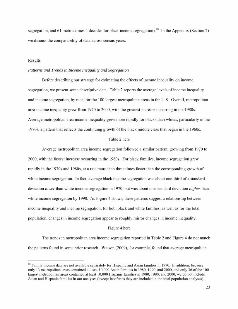
segregation, and 61 metros times 4 decades for black income segregation).18 In the Appendix (Section 2)

we discuss the comparability of data across census years.

Results

Patterns and Trends in Income Inequality and Segregation

Before describing our strategy for estimating the effects of income inequality on income

segregation, we present some descriptive data. Table 2 reports the average levels of income inequality

and income segregation, by race, for the 100 largest metropolitan areas in the U.S. Overall, metropolitan

area income inequality grew from 1970 to 2000, with the greatest increase occurring in the 1980s.

Average metropolitan area income inequality grew more rapidly for blacks than whites, particularly in the

1970s, a pattern that reflects the continuing growth of the black middle class that began in the 1960s.

Table 2 here

Average metropolitan area income segregation followed a similar pattern, growing from 1970 to

2000, with the fastest increase occurring in the 1980s. For black families, income segregation grew

rapidly in the 1970s and 1980s, at a rate more than three times faster than the corresponding growth of

white income segregation. In fact, average black income segregation was about one-third of a standard

deviation lower than white income segregation in 1970, but was about one standard deviation higher than

white income segregation by 1990. As Figure 4 shows, these patterns suggest a relationship between

income inequality and income segregation; for both black and white families, as well as for the total

population, changes in income segregation appear to roughly mirror changes in income inequality.

Figure 4 here

The trends in metropolitan area income segregation reported in Table 2 and Figure 4 do not match

the patterns found in some prior research. Watson (2009), for example, found that average metropolitan

18 Family income data are not available separately for Hispanic and Asian families in 1970. In addition, because only 13 metropolitan areas contained at least 10,000 Asian families in 1980, 1990, and 2000, and only 36 of the 100 largest metropolitan areas contained at least 10,000 Hispanic families in 1980, 1990, and 2000, we do not include Asian and Hispanic families in our analyses (except insofar as they are included in the total population analyses).

23

area income segregation of all families, as measured by the Centile Gap Index, declined slightly in the

1970s and 1990s but rose sharply in the 1980s. Jargowsky (1996) and Yang and Jargowsky (2006),

however, found that average metropolitan area income segregation of both white and black families, as

measured by the Neighborhood Sorting Index, rose in the 1970s and 1980s, but declined sharply in the

1990s. Our estimated trends differ from these for two primary reasons. First, we use a different measure

of income segregation than these prior studies, for reasons we describe above. Second, our estimates are

based on the 100 largest metropolitan areas, while Watson (2009) uses 216 metro areas; Jargowsky

(1996) uses 228 and 76 metropolitan areas for the white and black trends, respectively, from 1970-1990;

and Yang and Jargowsky (2006) use 324 and 130 metropolitan areas for the white and black trends,

respectively, from 1990-2000. Our restriction to the 100 largest metropolitan areas has substantial

implications for the estimated trends, as is evident in Figure 5, which shows trends in income inequality

and segregation for smaller metropolitan areas (those with at least 10,000 families of the relevant group in

each year, excluding the 100 largest metropolitan areas). For small metropolitan areas, the trends in

income inequality are very similar to those for large metropolitan areas, but the trends in income

segregation are quite different. Income segregation in small metropolitan areas is, on average, much

lower than for large metropolitan areas. In addition, income segregation in small metropolitan areas

declined in both the 1970s and 1990s (among all families and for white families). Pooling the trends for

large and small metropolitan areas would yield a trend similar to that described by Watson (2009)—

declining average income segregation in the 1970s and 1990s and a sharp increase in average income

segregation in the 1980s.

Figure 5 here

Although Table 2 and Figure 4 show changes in the average values of the rank-order information

theory index from 1970 to 2000, they do not provide detail on the extent to which changes in income

segregation are due to changes in the segregation of affluence and poverty. Figures 6-8 (for detail, see

Appendix Section 3, Table A1) show average metropolitan area segregation profiles for 1970-2000.

These enable us to examine the extent to which segregation has changed between the poor and non-poor

24

and the rich and non-rich, for example.

Figure 6 here

Figure 6 shows the trend in the average income segregation profile across the 100 largest

metropolitan areas from 1970-2000. First, note that in 1970, the poor were much less segregated from the

non-poor than the rich were from the non-rich. Income segregation between the poor and non-poor

(segregation of poverty) grew sharply between 1970 and 1980, however, while income segregation of the

rich and non-rich (segregation of affluence) did not. In the 1980s, however, income segregation grew at

all parts of the income distribution. In the 1990s, in contrast, income segregation grew only modestly,

and only between families in the middle part of the income distribution. On average, the segregation of

poverty and the segregation of affluence were relatively unchanged in the 1990s. These figures

demonstrate that a single measure of income segregation may not fully convey the pattern of changes.

Figures 7 and 8 show the corresponding trends for white (Figure 7) and black families (Figure 8)

separately. As we would expect, given the size of the white population, the trends for white income

segregation are similar to those of the population as a whole. The trends in black family income

segregation, however, are rather different. Black income segregation grew rapidly in the 1970s and 1980s

at all parts of the black income distribution. Not only did low-income black families become more

isolated from middle- and higher-income black families, but higher-income blacks became increasingly

segregated from lower-and middle-income black families as well. In the 1990s, this trend ceased

abruptly. In fact, the segregation of lower- and moderate-income black families from higher-income

black families declined slightly in the 1990s.

Figures 7 & 8 here

The tables and figures above describe patterns and trends in income segregation using “aspatial”

measures of segregation. These measures treat census tracts as discrete, spatially anonymous units and so

are not fully sensitive to changing spatial patterns of segregation. In particular, they are insensitive to the

spatial scale of segregation—they do not indicate the extent to which segregation levels are due to the

large or small scale spatial patterning of families in residential space. Figure 9 reports average

25

segregation profiles similar to those in Figures 6-8, but using the spatial information theory index

(Reardon & O'Sullivan, 2004) computed at a range of spatial scales instead of the tract-based information

theory index used in the figures above.

In particular, Figure 9 shows the average spatial information theory index household19 income

segregation threshold profile computed using radii of 500, 1000, 2000, and 4000 meters for the 100

largest metropolitan areas in 2000. These radii correspond roughly to local environments ranging from

‘pedestrian’ in size (500 m radius) to those that are considerably larger (4000 m radius)—the size of a

large high-school attendance zone, for example—larger in scale than the neighborhoods in which most

people attend church, shop, and do much of their socializing (Reardon, et al., 2008). In addition, Figure 9

shows the macro/micro segregation ratio (dashed line, with scale on the right-hand axis), which measures

the proportion of micro-scale segregation (segregation among 500m radius local environments) that is due

to macro-scale segregation patterns (segregation among 4000m radius environments). This ratio can be

interpreted as a measure of the geographic scale of segregation, with larger values indicating that more of

the measured segregation is due to the separation of groups over large distances (Reardon, et al., 2009;

Reardon, et al., 2008).

Figure 9 here

Two key patterns are evident in Figure 9. First, spatial income segregation patterns are very

similar to the aspatial patterns shown in Figure 6. Segregation of high-income households from other

households is, in general, higher than the segregation of low-income households from other households,

regardless of the radius at which segregation is measured. Second, this pattern appears to be largely, if

not entirely, due to the fact that upper-income households are much more segregated at a large geographic

scale than are lower-income households. For high-income households, 60% or more of segregation

patterns are due to macro-scale segregation—presumably the concentration of high-income households in

wealthy suburban and exurban areas. For low-income households, 40% or less of segregation patterns are

19 We are able to use household income for the spatial measures rather than family income because we do not analyze spatial patterns for black and white families separately. As noted above, family and household income segregation are highly correlated.

26

due to macro-scale segregation; this implies that the poor are less concentrated spatially than the wealthy

in most metropolitan areas.

In sum, our descriptive analyses reveal several important trends. First, average metropolitan area

income inequality and segregation both grew from 1970-2000, though the growth in income segregation

was much larger for black families than for white families. Second, income segregation grew at all parts

of the income distribution from 1970-2000, though at different times and at different rates for black and

white families. Most of the growth in income segregation occurred between 1970 and 1990.

Nonetheless, both the segregation of poverty and the segregation of affluence were much higher in 2000

than they had been in 1970 for white and black families alike. And third, the segregation of affluence is

generally greater than the segregation of poverty in the 100 largest metropolitan areas, a pattern that

appears to be driven by the macro-scale segregation of the highest earners from others. In the next

section of the paper, we investigate the extent to which variation in income inequality can explain these

patterns.

Estimating the Effects of Income Inequality on Income Segregation

We estimate the effect of income inequality on income segregation using a set of fixed-effects

regression models. The models rely on 644 metro-group-year cases, as noted above. Because each

observation in the data corresponds to a specific metropolitan area, decade, and race group, there are three

potential sources of variation in income inequality—variation across decades (within each metro-by-

group cell), variation among metropolitan areas (within each decade-by-group cell), and variation

between race groups (within each metro-by-decade cell).20 We use three different fixed effects models,

each relying on a different source of variation in income inequality, to estimate the effect of income

inequality on segregation over time, across race groups, and across metropolitan areas, respectively.

In addition we wish to ensure that our estimates of the effect of inequality on segregation are not

20 Only 61 of the 100 metropolitan areas have this latter variation, because we include observations for black families in the sample only for the 61 metropolitan areas where there are at least 10,000 black families in each of the four Census years.

27

biased by any confounding metropolitan-level covariates that are correlated with both inequality and

segregation. Based on previous research, we control for metropolitan demographic characteristics,

housing market pressures and housing stock, intra- and inter-metropolitan mobility, population growth,

labor market characteristics, and family structure21 (Abramson, Tobin, & VanderGoot, 1995; Jargowsky,

1996; Massey & Eggers, 1993; Pendall & Carruthers, 2003; Watson, 2009; Wheeler, 2006; Wilson,

1987). Notably, because the U.S. Census does not provide information on family wealth, we are unable

to include controls for metro- year- and race-specific aspects of the distribution of wealth in our models.

Although wealth is only modestly correlated with income, it plays a key role in residential location

because it enables families to buy housing in communities where their current income may be

insufficient, and provides a financial cushion during unstable times, such as temporary unemployment,

illness, or divorce, and so enables families to remain in their home when their income cannot support

them (Wolff, 2006). Nonetheless, research suggests that wealth may not be a significant factor in

neighborhood migration patterns (Sharkey, 2008), although it is a stronger predictor of neighborhood

choice for blacks than it is for non-Hispanic whites (Crowder, South, & Chavez, 2006).

In the first set of regression models (models 1 and 2), we estimate the effect of changes in

inequality on changes in segregation, including both metropolitan area-by-group fixed effects and decade

fixed effects. These m dels for o have the m

· Γ Δ , (4)

where indexes metropolitan areas, indexes race groups, indexes Census years, and where

and indicate the rank-order segregation and income inequality, respectively, in metropolitan area

for group in year . The models include metropolitan area-by-group (Γ ) and decade (Δ ) fixed

effects. The coefficient on inequality from this model indicates the average within-metro-group 21 More specifically, to control for these factors in our models, we include metropolitan-level population counts of each race group, percent older than 65 and younger than 18 years-old, percent with at least a high school diploma by race, percent foreign born, percent in the manufacturing sector, percent in the managerial/professional sector, percent in finance, insurance, and real estate, percent in the construction sector, percent unemployed by race, per capita income by race, intra- and inter-metropolitan mobility, percent new housing construction, and percent female-headed households by race. The data sources for and construction of each of these variables are described in the Appendix (Section 2) in more detail.

28

association (over time) between inequality and segregation, net of any secular trend common to all

metropolitan areas and race groups. Model 2 includes a set of metro-year and group-metro-year

covariates ( and ) as control variables in addition to the fixed effects. We compute

bootstrapped standard errors in all of the regression models to take into account the clustered nature of the

observations.

In the second set of models (Model 3 and 4), we estimate the effect of differences in income

inequality between race groups on income segregation, using metropolitan area-by-year fixed effects and

group-specific dummy vari les. od s hav he fab These m el e t orm

· Γ Δ , (5)

where Γ and Δ are metropolitan area-by-year and group-specific fixed effects, respectively. The

coefficient on inequality from this model indicates the average within-metro-year association (between

race groups) between inequality and segregation, net of any average differences in inequality and

segregation between race groups across metropolitan areas and time. Model 4 includes a small set of

group-metro-year covariates as control variables as well as the fixed effects.

In the third set of models (Model 5 and 6), we estimate the effect of differences in income

inequality among racial groups on income segregation, using metropolitan area and group-by-year fixed

effects. These models have the form

· Γ Δ , ) (6

where Γ and Δ are group-by-year and metropolitan area fixed effects, respectively. The coefficient

on inequality from this model indicates the average within-group-year association (across metropolitan

areas) between inequality and segregation, net of any average differences in inequality and segregation

among metropolitan areas across groups and decades. Model 6 includes a set of group-metro-year and

metro-year covariates as control variables as well as the fixed effects. Because the three models rely on

different sources of variation in income inequality, each relies on a different key assumption in order to

29

support a causal claim about the effect of income inequality on income segregation.22 As a result, if the

three sets of models produce similar results, we can rule out many potential sources of bias. As an

additional set of sensitivity checks, we estimate a set of models for each race group separately, and a set

for each decade separately.

Main Effects of Income Inequality on Income Segregation

Table 3 reports the estimates from the models described in Equations (3)-(5) above. Of primary

interest here are the estimated coefficients on the Gini index in Models 2, 4, and 6, which include the full

set of covariates as well as the fixed effects. Model 2 yields an estimated association of 0.467 (s.e.=

0.060; p<.001) between income inequality and income segregation, net of the model’s fixed effects and

covariates. In other words, a change of one point in a group’s income inequality is associated with a

change of roughly a half a point in income segregation. Note also that Model 1 implies that changes in

income inequality alone do not fully explain the trends in income segregation—even after controlling for

income inequality, within-group income segregation grew, on average, by 0.013 points in the 1970s and

by another 0.015 points in the 1980s.

Table 3 here

Model 4, which relies on variation in income inequality between white and black families within

the same metropolitan area and year, yields an estimated association between inequality and segregation

22 The models that include metro-by-group fixed effects rely on the assumption that changes in income inequality within a metropolitan area and race group over time are exogenous, conditional on secular trends common to all groups and metropolitan areas and the set of included covariates in the model. The models that include metro-by-year fixed effects rely on the assumption that differences between white and black income inequality within the same metropolitan area and decade are exogenous, once we have accounted for differences in income inequality between white and black families that are common across metropolitan areas and time and differences in inequality that are associated with differences in the covariates included in the model. And finally, the models that include group-by-year and metropolitan area fixed effects rely on the assumption that differences in income inequality within a given year and for a given race group are exogenous, once we have accounted for stable differences among metropolitan areas and differences associated with the covariates in the model. None of these three assumptions are likely to be perfectly true, but each model is somewhat insulated against threats to another. If we are worried about temporal confounding biasing the estimates from the first models, for example, we can examine the second and third set of models, each of which relies on cross-sectional variation across groups or metropolitan areas. If we are worried about unobserved group-specific factors, such as a correlation between employment sector and preferences for neighbors, biasing the estimates in the second set of models, we can look to the first and third set of models, each of which relies only on within-group variation (over time or across metropolitan areas).

30

of 0.783 (s.e.=0.125; p<.001), somewhat larger than the estimate from model 2. Note that Model 3

implies that income inequality alone more than accounts for the differences in income segregation

between black and white families. Model 3 implies that income segregation among black families is

lower, on average, than among white families within the same metropolitan area and year, given the same

level of income inequality.

Finally, Model 6 yields an estimated association between income inequality and income

segregation of 0.502 (s.e.=0.110; p<.001). Thus, each of the three models yields estimated coefficients on

income inequality that imply inequality has a positive effect on income segregation. To get a sense of the

magnitude of these effects, note that an effect of 0.500 (roughly that found in Models 2 and 6) implies

that the changes in income inequality from 1970 to 2000 shown in Table 2 account for roughly 40% of

the average change in black income segregation, 80% of the average change in white income segregation,

and 60% of the average change in overall income segregation. Put differently, a one-standard deviation

change in income inequality leads to roughly one-quarter of a standard deviation change in income

segregation.23

To ensure that the estimates from Models 2, 4, and 6 are not driven by one particular race group

or decade, we fit an additional set of models for each race group separately, and another set of models for

each decade separately. The results of these models are shown in Table 4. In each model, the coefficient

on inequality is positive and statistically significant. In the group-specific models, the coefficients range

from 0.450 to 0.561; in the decade-specific models, the coefficients range from 0.624 to 0.732. Thus,

across all the models shown in Tables 3 and 4, we find that income inequality has a large and positive

association with income segregation, regardless of whether we rely on temporal, between-group, or

between-metropolitan area variation to identify this association, and regardless of which groups or

23 These are computed from the 1970-2000 changes in inequality and segregation shown in Table 2. For example, income inequality among all families grew by 0.048 from 1970-2000. If the effect of income inequality on segregation were 0.500, this would imply a change in income segregation of 0.048 · 0.5 0.024, which is roughly 70% of the observed total change (0.033) in income segregation from 1970-2000. Likewise, the standard deviation of income inequality within a given year was roughly 0.025, on average, while the standard deviation of income segregation was roughly 0.050. This implies that an effect of 0.500 corresponds to an effect size of 0.25.

31

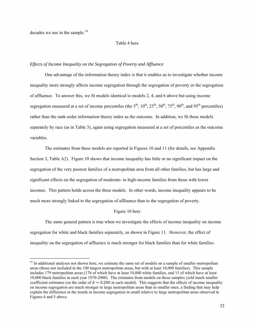
decades we use in the sample.24

Table 4 here

Effects of Income Inequality on the Segregation of Poverty and Affluence

One advantage of the information theory index is that it enables us to investigate whether income

inequality more strongly affects income segregation through the segregation of poverty or the segregation

of affluence. To answer this, we fit models identical to models 2, 4, and 6 above but using income

segregation measured at a set of income percentiles (the 5th, 10th, 25th, 50th, 75th, 90th, and 95th percentiles)

rather than the rank-order information theory index as the outcome. In addition, we fit these models

separately by race (as in Table 3), again using segregation measured at a set of percentiles as the outcome

variables.

The estimates from these models are reported in Figures 10 and 11 (for details, see Appendix

Section 3, Table A2). Figure 10 shows that income inequality has little or no significant impact on the

segregation of the very poorest families of a metropolitan area from all other families, but has large and

significant effects on the segregation of moderate- to high-income families from those with lower

incomes. This pattern holds across the three models. In other words, income inequality appears to be

much more strongly linked to the segregation of affluence than to the segregation of poverty.

Figure 10 here

The same general pattern is true when we investigate the effects of income inequality on income

segregation for white and black families separately, as shown in Figure 11. However, the effect of

inequality on the segregation of affluence is much stronger for black families than for white families.

24 In additional analyses not shown here, we estimate the same set of models on a sample of smaller metropolitan areas (those not included in the 100 largest metropolitan areas, but with at least 10,000 families). This sample includes 179 metropolitan areas (176 of which have at least 10,000 white families, and 15 of which have at least 10,000 black families in each year 1970-2000). The estimates from models on these samples yield much smaller coefficient estimates (on the order of 0.200 in each model). This suggests that the effects of income inequality on income segregation are much stronger in large metropolitan areas than in smaller ones, a finding that may help explain the difference in the trends in income segregation in small relative to large metropolitan areas observed in Figures 4 and 5 above.

32

That is, in metropolitan areas and years when black income inequality is largest, the highest-earning 10

percent of black families are much more segregated from the lower 90 percent of black families than

when and where black income inequality is low.

Figure 11 here

Effects of Income Inequality on Spatial Segregation Patterns

Our third set of analyses investigates whether income inequality produces macro- and/or micro-

scale income segregation patterns. For these analyses, we focus on the relationship between overall

income inequality and household income segregation, rather than race-specific family income inequality

and segregation. As above, we focus on the 100 largest metropolitan areas in 2000. We fit models that

include metropolitan area and year fixed effects and a set of metropolitan area-by-year covariates (the

models are identical to those specified in Column 1 of Table 4, save for the different outcome and the fact

that we use data only from years 1980-2000).

In order to investigate the geographic scale of the effects of income inequality, we fit these

models using five different measures of spatial segregation: four using different radii and one using the

measure of “net micro segregation” described by Lee et al (2008). Our rationale for this is as follows.

The level of segregation among micro-environments (local environments of 500 meter radius) can be

thought of as made up of two non-negative components: a component that is due to macro-scale

segregation patterns—that is, segregation among macro-environments (local environments of 4000 meter

radius)—plus a component that is due to micro-scale variation in neighborhood composition over and

above the macro-scale patterns. By definition, then, the effect of inequality on segregation among micro-

scale environments will be equal to the sum of its effect on macro-scale segregation and its effect on net

micro segregation. Thus, by comparing the effect estimates across the outcome measures, we can infer

the geographic scale at which income inequality affects segregation. For example, if inequality affects

segregation among micro-environments much more than it affects segregation among macro-

environments, then the effect of segregation must operate primarily to increase the small-scale spatial

33

patterning of income (net micro segregation). Conversely, if inequality affects segregation among micro-

and macro-scale environments equally, then the effect of segregation must operate primarily to increase

the macro-scale spatial patterning of income (and have no effect on small-scale pattering).

Our estimates of these different effects are shown in Table 5. The key result in Table 5 is the

consistency of the point estimates of the effect of inequality (reading across rows of the Table), regardless

of the radius used to define a household’s local environment. In each model, and regardless of the span of

years, income inequality has a significant effect on macro-scale segregation (4000-meter-radius local

environments), and a roughly similar-sized effect on smaller-scale segregation (though the latter estimates

are not always statistically significant due to large standard errors). Moreover, the effect of income

inequality on net micro-scale segregation (the difference between 500-meter and 4000-meter radius

segregation, shown in the 5th column of Table 5) is indistinguishable from zero in these models, implying

that the effect of income inequality on segregation operates entirely through its effect on macro

segregation. In other words, income inequality affects income segregation by shaping residential patterns

at a large spatial scale, rather than by increasing the block-to-block sorting of households by income.

Table 5 here

In Figure 12, we present the results of an analysis that combines features of two of the preceding

analyses. Here we report the effects of income inequality on spatial household income segregation at

specific percentiles of the income distribution and using different local environment radii to compute

spatial segregation. The left-hand panel of Figure 12 shows that income inequality has a large positive

effect on the spatial segregation of affluence but a negative effect on the spatial segregation of extreme

poverty (the bottom 5% of the income distribution) when segregation is computed among local

environments of 500 meter radius. The center panel indicates that income inequality has a similar effect

on macro-scale segregation, except in the bottom quartile of the income distribution. The right-hand

panel of Figure 12 describes the portion of the effect of income inequality on 500-meter radius

segregation that is not due to macro-scale segregation effects (mathematically, this effect is the difference

between the two effects in the left and center of the Figure). Except for the effects on the segregation of

34

poverty, these net-micro-scale effects are indistinguishable from zero. Income inequality does, however,

appear to reduce the segregation of extreme poverty by reducing the small-scale patterning of the

segregation of the very poor, a finding consistent with the fact that income inequality may actually

compress the lower part of the income distribution. As we note above, when the lower part of the income

distribution is compressed, low-income households at different percentiles of the income distribution may

be more likely to be able to afford to live in the same neighborhoods, leading to lower income

segregation. In sum, Figure 12 suggests that income inequality affects income segregation primarily by

increasing the macro-scale separation of the affluent from all others. As income inequality grows, this

suggests, the middle and upper-middle class become increasingly concentrated together at relatively large

distances from those with lower incomes.

Figure 12 here

Discussion and Conclusions

Our analysis yields four main findings. First, we reproduce the finding in Watson (2009) and

Mayer (2001b) linking income inequality to income segregation. Using a set of fixed-effects regression

models, we show that there is a strong and robust relationship between within-race metropolitan area

income inequality and within-race metropolitan area income segregation, net of secular trends, stable

between-race differences, and stable differences among metropolitan areas. Our estimates indicate that a

one standard deviation increase in income inequality leads to a quarter of a standard deviation increase in

income segregation, an effect roughly half the size of that found by Watson (2009). Nonetheless, these

effects are large enough to be substantially meaningful—they imply that increasing income inequality

was responsible for 40-80% of the changes in income segregation from 1970-2000. The strength and

consistency of our results across a wide range of model specifications suggests this is a robust

relationship, at least among large metropolitan areas in the decades from 1970-2000. The estimated

effect, however, is much weaker among small metropolitan areas. Moreover, it is important to keep in

mind that this analysis investigates the effect of income inequality in an era of rising inequality. It is not

35

clear to what extent these findings generalize to eras of lower, or stable, inequality.

One might be concerned that our estimated effects are subject to various forms of bias. For

example, despite our efforts to use a range of modeling strategies to protect our estimates from

unobserved confounding, the estimated associations here may nonetheless be biased by the presence of

some unaccounted-for factors that shape both income inequality and income segregation. The

consistency of the results across three sources of variation, however, strongly suggest a causal

relationship. More importantly, one might worry that the estimated associations represent the effects of

segregation on inequality, rather than the other way around. Certainly there is reason to suspect that

income segregation may engender increased income inequality, by providing differential access to quality

schooling, high-paying labor markets, and differential social capital. However, many mechanisms that

would drive such effects would require considerable time to take effect (schooling effects would not

manifest as increased income inequality for many years, for example), so we think these are less plausible

explanations for our findings. Nonetheless, we test the hypothesis of reverse causality by reversing our

regressions (using inequality as the dependent variable and segregation as an independent variable in

Models 2, 4, and 6). In each case, the estimated associations between segregation and inequality are

positive and statistically significant, but much smaller in magnitude than the effects we report.25

Our second main finding is that income inequality affects income segregation primarily by

affecting the segregation of affluence, rather than the segregation of poverty. Although the segregation of

poverty increased from 1970-2000 for both white and black families, as well as for all families, very little

of this change is attributable to changes in income inequality. Indeed, income inequality affects the

relative incomes of lower-income households only to a small degree—and may actually compress the low

end of the income distribution. This suggests that changes in income inequality would be expected to

have little effect on the segregation of poverty. Our estimates of the effect of income inequality on spatial

segregation, in fact, suggest that income inequality may slightly reduce the spatial segregation of low-

25 While inequality explains 1/2-2/3 of the variation in segregation, segregation only explains 1/5 of the variation in inequality.

36

income households. Given that income inequality does not seem to drive the patterns of the segregation

of poverty, we suspect that the segregation of poverty is more a result of housing policy than of income

inequality. Through the 1980s, federal and metropolitan housing policies fostered the development of

high-density housing for low-income families. These policies are likely responsible for much of the

growth of the segregation of poverty over that time. Likewise, the growth in scattered site low-income

and mixed-income housing in the 1990s, coupled with the demolition of some large, high-density public

housing projects, may account for the stabilization of the segregation of poverty in the 1990s.

Third, we find that the relationship between income inequality and income segregation differs for

black and white families. In 1970, income segregation among black families was lower than among white

families. This is likely the result of the ghettoization of minorities that took place, particularly in

Northern and Midwestern American cities, during the post-WWII suburbanization boom. Because of

housing discrimination, black families were largely denied access to suburban areas, leaving both middle-

and lower-income black families living in relative proximity in urban areas. The passage of housing and

lending anti-discrimination legislation in the 1970s, however, began to reduce the prevalence of housing

discrimination, making a wider range of neighborhood options available to middle-income black families.

As a result, income segregation among black families rose steeply from 1970-1990, as the growing black

middle class was able to move into previously inaccessible suburban areas. By 1980, in fact, income

segregation among black families was higher than among white families. In this era, black income

inequality is strongly related to the segregation of high-income black families in neighborhoods separate

from lower-income black families. Although this growth in income segregation among black families is a

result of both the growing black middle class and reductions in housing discrimination—both signs of

progress since the 1960s—it nonetheless may have negative consequences. Given high levels of racial

segregation in U.S. cities, the growth of income segregation among black families results in the increasing

racial and socioeconomic isolation of lower-income black families in neighborhoods of concentrated

disadvantage (Wilson, 1987).

Finally, we find that the effects of income inequality on income segregation are driven primarily

37

by the effects of inequality on macro-scale patterns of segregation. Coupled with our earlier finding

regarding the effects of inequality on the segregation of affluence, this means that income inequality

appears to increase income segregation largely by inducing the highest-earning families to move far away

from lower-income households. The expansion of suburban and exurban areas in the last few decades,

facilitated by the growth of the highway system and the movement of many high-skill industries to the

suburban ring, has allowed families to move farther away from metropolitan cores while still engaging in

the high-skill labor market. The fact that the effect of income inequality on income segregation is much

weaker in small metropolitan areas is consistent with this explanation. Because macro-scale segregation

is often not possible in small metropolitan areas, inequality may have little room to affect income

segregation. If one of the key amenities that high-income families desire to purchase is space—large lots,

very low-density housing, and access to parks and undeveloped open space—then they will be much more

able to do so in large metropolitan areas.

In sum, our analyses show that income inequality has a strong and robust effect on income

segregation, but that this effect is more nuanced in form that one might initially expect. In fact, income

inequality appears to be responsible for a specific aspect of income segregation—the large-scale

separation of the affluent from lower-income households and families. It does not, however, appear to be

responsible for patterns of segregation of poverty (for that, housing policy is likely to blame). Nor is it

responsible for patterns of small-scale income segregation, such as those seen resulting from the

gentrification of urban neighborhoods adjacent to poor, non-gentrifying neighborhoods.

The macro-scale spatial segregation of high-income households from middle- and low-income

households may have important and far-reaching consequences, particularly given that the top 10% of

earners in the U.S. now receive 45% of all income. The segregation of these high-income households in

communities spatially far from lower-income households may reduce the likelihood that high-income

residents will have social, or even casual, contact with lower-income residents. This in turn may make it

less likely that they are willing to invest in metropolitan-wide public resources that would benefit

residents of all income levels, such as transportation networks, utilities, parks, services, and cultural

38

amenities. Moreover, the spatial separation of the affluent and poor implies that there will be few

opportunities for disadvantaged families to benefit from local spillover of public goods. The distance

between affluent and lower-income communities make it unlikely that disadvantaged families will be able

to take advantage of the local schools, parks, and services in which affluent communities invest.

Although most sociological theory and research regarding the spatial distribution of income has focused

on the effects of concentrated poverty on residents of poor neighborhoods, the findings here suggest that a

better understanding of the effects of concentrated affluence on residents far from affluent communities is

needed as well. The segregation of affluence may directly affect the resources available to residents of

both poor and lower-income neighborhoods.

Given the evidence that income inequality has sizeable effects on income segregation, it is

plausible that income segregation may mediate the effects of income inequality on social outcomes. A

large body of research has linked income inequality to negative health outcomes such as increased

morbidity, mortality, and infant death, as well as to negative effects on educational attainment, crime

rates, social capital, network ties, and political institutions (see Neckerman & Torche, 2007 for a review).

Although some scholars have argued that income segregation may serve as a mechanism that links

income inequality to some of these negative social outcomes (Mayer, 2002; Mayer & Sarin, 2005;

Neckerman & Torche, 2007), the scant research on this topic has produced mixed results. Mayer and

Sarin (2005) explicitly test this hypothesis and show that income segregation is one mechanism that links

income inequality to infant mortality at the state level. On the other hand, other research finds that

economic segregation does not mediate the relationship between income inequality and mortality

(Lobmayer & Wilkinson, 2002) or between income inequality and the distribution of educational

attainment (Mayer, 2001a). Clearly the role of income segregation as a mediator between income

inequality and various social outcomes warrants further investigation, as does the direct impact of income

segregation on other forms of social inequality.

   

39

References Abramson, A. J., Tobin, M. S., & VanderGoot, M. R. (1995). The changing geography of metropolitan

opportunity: The segregation of the poor in U.S. metropolitan areas, 1970 to 1990. Housing

Policy Debate, 6(1), 45-72.

Ananat, E. O. (2007). The wrong side(s) of the tracks: estimating the causal effects of racial segregation

on city outcomes (Working Paper No. 13343): National Bureau of Economic Research.

Autor, D. H., Katz, L. H., & Kearney, M. S. (2006). The Polarization of the U.S. Labor Market. American

Economic Review, 95(2), 189-194.

Autor, D. H., Katz, L. H., & Kearney, M. S. (2008). Trends in U.S. Wage Inequality: Revising the

Revisionists. The Review of Economics and Statistics, 90(2), 300-323.

Burkhauser, R. V., Feng, S., Jenkins, S. P., & Larrimore, J. (2009). Recent trends in top income shares in

the USA: Reconciling estimates from March CPS and IRS tax return data (NBER Working Paper

#15320). Cambridge, MA: National Bureau of Economic Research.

Card, D., & DiNardo, J. E. (2002). Skill-biased technological change and rising wage inequality: some

problems and puzzles. Journal of Labor Economics, 20(4), 733-783.

Card, D., Lemieux, T., & Riddell, W. C. (2004). Unions and wage inequality. Journal of Labor Research,

25(4), 519-559.

Clampet-Lundquist, S., & Massey, D. S. (2008). Neighborhood Effects on Economic Self‐Sufficiency: A

Reconsideration of the Moving to Opportunity Experiment. American Journal of Sociology,

114(1), 107-143.

Coulton, C. J., Chow, J., Wang, E. C., & Su, M. (1996). Geographic concentration of affluence and

poverty in 100 metropolitan areas, 1990. Urban Affairs Review, 32, 186-216.

Crowder, K., South, S., & Chavez, E. (2006). Wealth, Race, and Inter-Neighborhood Migration.

American Sociological Review, 71, 72–94.

Cutler, D. M., & Glaeser, E. L. (1997). Are ghettos good or bad? Quarterly Journal of Economics,

112(3), 827-871.

40

Davidoff, T. (2005). Income sorting: Measurement and decomposition (Working paper). Berkeley, CA:

UC-Berkeley.

DiPrete, T. A. (2007). What Has Sociology to Contribute to the Study of Inequality Trends? A Historical

and Comparative Perspective. American Behavioral Scientist, 50(5), 603-618.

Duncan, O. D., & Duncan, B. (1955). A methodological analysis of segregation indexes. American

Sociological Review, 20(2 (April)), 210-217.

Durlauf, S. (1996). A Theory of Persistent Income Inequality. Journal of Economic Growth, 1, 75-93.

Echenique, F., & Fryer, R. G. (2005). On the measurement of segregation.

Ellen, I. G. (2000). Is segregation bad for your health? The case of low birth weight. Brookings-Wharton

Papers on Urban Affairs, 203-238.

Farley, R., & Frey, W. H. (1994). Changes in the segregation of whites from blacks during the 1980s:

Small steps toward a more integrated society. American Sociological Review, 59(February), 23 -

45.

Firebaugh, G., & Schroeder, M. B. (2007). Does your neighbor's income affect your happiness? (mimeo).

Fong, E., & Shibuya, K. (2000). The spatial separation of the poor in Canadian cities. Demography,

37(4), 449-459.

GeoLytics. (2004). Neighborhood Change Database. East Brunswick, NJ: GeoLytics, Inc.

Gottschalk, P., & Danziger, S. (2005). Inequality of wage rates, earnings and family income in the United

States, 1975–2000. Review of Income and Wealth, 51, 231-254.

Hardman, A., & Ioannides, Y. M. (2004). Neighbors' income distribution: Economic segregation and

mixing in U.S. urban neighborhoods. Journal of Housing Economics, 13, 368-382.

Ioannides, Y. M. (2004). Neighborhood income distributions. Journal of Urban Economics, 56(3), 435-

457.

Ioannides, Y. M., & Seslen, T. N. (2002). Neighborhood wealth distributions. Economics Letters, 76,

357-367.

James, D. R., & Taeuber, K. E. (1985). Measures of segregation. Sociological Methodology, 14, 1-32.

41

Jargowsky, P. A. (1996). Take the money and run: Economic segregation in U.S. metropolitan areas.

American Sociological Review, 61(6), 984-998.

Jargowsky, P. A. (1997). Poverty and place: Ghettos, barrios, and the American city. New York: Russell

Sage Foundation.

Jargowsky, P. A. (2003). Stunning progress, hidden problems: The dramatic decline of concentrated

poverty in the 1990s (Report). Washington, DC: Brookings Institution.

Jencks, C., & Mayer, S. (1990). The social consequences of growing up in a poor neighborhood. In L. E.

Lynn, Jr. & M. G. H. McGeary (Eds.), Inner-city poverty in the United States (pp. 111-186).

Washington, DC: National Academy Press.

Jenkins, S. P., Micklewright, J., & Schnepf, S. V. (2006). Social segregation in schools: An international

comparison. Paper presented at the 29th General Conference of The International Association for

Research in Income and Wealth, Joensuu, Finland.

Katz, L. F., Kling, J. R., & Liebman, J. B. (2007). Experimental estimates of neighborhood effects.

Econometrica, 75(1), 83-119.

Lee, B. A., Reardon, S. F., Firebaugh, G., Farrell, C. R., Matthews, S. A., & O'Sullivan, D. (2008).

Beyond the Census Tract: Patterns and Determinants of Racial Residential Segregation at

Multiple Geographic Scales. American Sociological Review, 73, 766-791.

Lee, D. S. (1999). Wage Inequality in The United States During The 1980s: Rising Dispersion Or Falling

Minimum Wage? The Quarterly Journal of Economics, 114(3), 977-1023.

Leventhal, T., & Brooks-Gunn, J. (2000). The neighborhoods they live in: The effects of neighborhood

residence on child and adolescent outcomes. Psychological Bulletin, 126(2), 309-337.

Levy, F., & Murnane, R. J. (1992). U.S. earnings levels and earnings inequality: a review of recent trends

and proposed explanations. Journal of Economic Literature, 30(September), 1333-1381.

Lobmayer, P., & Wilkinson, R. (2002). Inequality, residential segregation by income, and mortality in US

cities. Journal of Epidemiology and Community Health, 56, 183-187.

42

Ludwig, J., Liebman, J. B., Kling, J. R., Duncan, G. J., Katz, L. F., Kessler, R. C., et al. (2008). What Can

We Learn about Neighborhood Effects from the Moving to Opportunity Experiment? American

Journal of Sociology, 114(1), 144-188.

Massey, D. S. (1996). The age of extremes: Concentrated affluence and poverty in the twenty-first

century. Demography, 33(4), 395-412.

Massey, D. S., & Denton, N. A. (1988). The dimensions of residential segregation. Social Forces, 67(2),

281-315.

Massey, D. S., & Eggers, M. L. (1993). The spatial concentration of affluence and poverty during the

1970s. Urban Affairs Quarterly, 29, 299-315.

Massey, D. S., & Fischer, M. J. (2003). The geography of inequality in the United States, 1950-2000.

Brookings-Wharton Papers on Urban Affairs(4), 1-40.

Mayer, S. E. (2000). Income Inequality, Economic Segregation and Children's Educational Attainment

(Working Paper No. 00.26). Chicago, IL: University of Chicago.

Mayer, S. E. (2001a). How did the increase in economic inequality affect educational attainment?

American Journal of Sociology, 107, 1-32.

Mayer, S. E. (2001b). How the growth in income inequality increased economic segregation. Joint Center

for Poverty Research, Working Paper 230.

Mayer, S. E. (2002). How economic segregation affects children's educational attainment. Social Forces,

81, 153-176.

Mayer, S. E., & Sarin, A. (2005). An assessment of some mechanisms linking economic inequality and

infant mortality. Social Science and Medicine, 60(439-55).

Minnesota Population Center. (2004). National Historical Geographic Information System: Pre-release

Version 0.1. Minneapolis, MN: University of Minnesota. http://www.nhgis.org.

Moller, S., Alderson, A. S., & Nielsen, F. (2009). Changing Patterns of Income Inequality in U.S.

Counties, 1970–2000. American Journal Of Sociology, 114(4), 1037-1101.

43

Mora, R., & Ruiz-Castillo, J. (2003). Additively Decomposable Segregation Indexes. The Case of Gender

Segregation by Occupations and Human Capital Levels in Spain. Journal of Economic Inequality,

1(2), 147-179.

Morenoff, J. D. (2003). Neighborhood Mechanisms and the Spatial Dynamics of Birth Weight. American

Journal of Sociology, 108(5), 976–1017.

Neckerman, K. M., & Torche, F. (2007). Inequality: Causes and Consequences. The Annual Review of

Sociology, 33, 335-357.

Nielsen, F., & Alderson, A. S. (1997). The Kuznets curve and the great u-turn: Income inequality in U.S.

counties, 1970 to 1990. American Sociological Review, 62(1), 12-33.

Osypuk, T. L., & Acevedo-Garcia, D. (2008). Are Racial Disparities in Preterm Birth Larger in

Hypersegregated Areas? American Journal of Epidemiology, 167(11), 1295-1304.

Pendall, R., & Carruthers, J. I. (2003). Does density exacerbate income segregation? Evidence from U.S.

metropolitan areas, 1980 to 2000. Housing Policy Debate, 14(4), 541-589.

Pielou, E. C. (1977). Mathematical ecology (2nd ed.). New York: John Wiley & Sons.

Piketty, T., & Saez, E. (2003). Income Inequality in the United States, 1913-1998. The Quarterly Journal

of Economics, 118(1), 1-39.

Piketty, T., & Saez, E. (2008). Income Inequality in the United States, 1913-1998 (Tables and figures

updated to 2006). Retrieved 2 September, 2009, from

http://www.econ.berkeley.edu/~saez/TabFig2006.xls

Quillian, L. (2007). Does Segregation Create Winners and Losers? Education and Spatial Segregation on

the Basis of Income and Race. Paper presented at the Annual Meeting of the Population

Association of America.

Reardon, S. F., Farrell, C. R., Matthews, S., O'Sullivan, D., Bischoff, K., & Firebaugh, G. (2009). Race

and Space in the 1990s: Changes in the Geographic Scale of Racial Residential Segregation,

1990-2000. Social Science Research, 38, 55-70.

44

Reardon, S. F., & Firebaugh, G. (2002). Measures of multi-group segregation. Sociological Methodology,

32, 33-67.

Reardon, S. F., Firebaugh, G., O'Sullivan, D., & Matthews, S. A. (2006, August 20-26, 2006). Measures

of socioeconomic segregation. Paper presented at the 29th General Conference of the

International Association for Research in Income and Wealth, Joensuu, Finland.

Reardon, S. F., Matthews, S. A., O'Sullivan, D., Lee, B. A., Firebaugh, G., Farrell, C. R., et al. (2008).

The geographic scale of metropolitan racial segregation. Demography, 45, 489-514.

Reardon, S. F., & O'Sullivan, D. (2004). Measures of spatial segregation. Sociological Methodology, 34,

121-162.

Rosenbaum, J. E., & Popkin, S. J. (1991). Employment and earnings of low-income blacks who move to

middle-class suburbs. In C. Jencks & P. E. Peterson (Eds.), The urban underclass (pp. 342-356).

Washington, DC: Brookings Institution.

Ross, S. L., & Turner, M. A. (2005). Housing Discrimination in Metropolitan America: Explaining

Changes Between 1989 and 2000. Social Problems, 52, 152-180.

Ryscavage, P. (1999). Income Inequality in America: An Analysis of Trends. New York: M. E. Sharpe.

Sampson, R. J. (2008). Moving to Inequality: Neighborhood Effects and Experiments Meet Social

Structure. American Journal of Sociology, 114(1), 189-231.

Sampson, R. J., Morenoff, J. D., & Earls, F. (1999). Beyond social capital: Spatial dynamics of collective

efficacy for children. American Sociological Review, 64(5), 633-660.

Sampson, R. J., Raudenbush, S. W., & Earls, F. (1997). Neighborhoods and violent crime: A multilevel

study of collective efficacy. Science, 277, 918-924.

Sampson, R. J., Raudenbush, S. W., & Sharkey, P. (2008). Durable effects of concentrated disadvantage

on verbal ability among African-American children. Proceedings of the National Academy of

Sciences, 105(3), 845-852.

Schwartz, C. R., & Mare, R. D. (2005). Trends in Educational Assortative Marriage from 1940-2003.

Demography, 42, 621-646.

45

Sharkey, P. (2008). The Intergenerational Transmission of Context. American Journal of Sociology,

113(4), 931–969.

Son, I. S., Model, S. W., & Fisher, G. A. (1989). Polarization and Progress in the Black Community:

Earnings and Status Gains for Young Black Males in the Era of Affirmative Action. Sociological

Forum, 4(3), 309-327.

South, S. J., & Crowder, K. D. (1998). Housing discrimination and residential mobility: Impacts for

blacks and whites. Population Research and Policy Review, 17, 369-387.

Taeuber, K. E., & Taeuber, A. F. (1965). Negroes in cities: Residential segregation and neighborhood

change. Chicago, IL: Aldine Publishing Co.

Theil, H. (1972). Statistical decomposition analysis (Vol. 14). Amsterdam: North-Holland Publishing

Company.

Theil, H., & Finezza, A. J. (1971). A note on the measurement of racial integration of schools by means

of informational concepts. Journal of Mathematical Sociology, 1, 187-194.

Tiebout, C. M. (1956). A pure theory of local expenditures. Journal of Political Economy, 64(October),

416-424.

Turner, M. A., & Ross, S. L. (2005). How Racial Discrimination Affects the Search for Housing. In X. d.

S. Briggs (Ed.), The Geography of Opportunity: Race and Housing Choice in Metropolitan

America (pp. 81-100). Washington, DC: Brookings Institution Press.

Turner, M. A., Ross, S. L., Galster, G. C., & Yinger, J. (2002). Discrimination in Metropolitan Housing

Markets: National Results from Phase I HDS 2000 [Electronic version]. from

http://www.huduser.org/publications/hsgfin/hds.html

Waitzman, N. J., & Smith, K. R. (1998a). Phantom of the Area: Poverty-Area Residence and Mortality in

the United States. American Journal of Public Health, 88(6), 973-976.

Waitzman, N. J., & Smith, K. R. (1998b). Separate but lethal: The effects of economic segregation on

mortality in metropolitan America. The Milbank Quarterly, 76(3), 341-373.

46

Watson, T. (2006). Metropolitan growth, inequality, and neighborhood segregation by income (Working

paper). Williamstown, MA: Williams College.

Watson, T. (2009). Inequality and the Measurement of Residential Segregation by Income. Review of

Income and Wealth, 55, 820-844.

Western, B., Bloome, D., & Percheski, C. (2008). Inequality among American Families with Children,

1975-2005. American Sociological Review, 73(December), 903-920.

Wheeler, C. H. (2006). Urban decentralization and income inequality: Is sprawl associated with rising

income segregation across neighborhoods? (FRB of St. Louis Working paper No. 2006-037A).

St. Louis, MO: Federal Reserve Bank of St. Louis.

Wheeler, C. H., & La Jeunesse, E. A. (2006). Neighborhood income inequality (FRB of St. Louis

Working paper No. 2006-039A). St. Louis, MO: Federal Reserve Bank of St. Louis.

Wheeler, C. H., & La Jeunesse, E. A. (2008). Trends in neighborhood income inequality in the U.S.,

1980-2000. Journal of Regional Science, 48(5), 879-891.

Wilson, W. J. (1987). The truly disadvantaged: The inner city, the underclass, and public policy.

Chicago: University of Chicago Press.

Wolff, E. N. (2006). Changes in Household Wealth in the 1980s and 1990s in the U.S. In E. N. Wolff

(Ed.), International Perspectives on Household Wealth. Northampton, MA: Elgar Publishing Ltd.

Wong, D. W. S. (1993). Spatial indices of segregation. Urban Studies, 30(3), 559-572.

Wong, D. W. S. (2002). Spatial measures of segregation and GIS. Urban Geography, 23(1), 85-92.

Yang, R., & Jargowsky, P. A. (2006). Suburban development and economic segregation in the 1990s.

Journal of Urban Affairs, 28(3), 253-273.

Yinger, J. (1995). Closed Doors, Opportunities Lost: The Continuing Costs of Housing Discrimination.

New York: Russell Sage Foundation.

Zoloth, B. S. (1976). Alternative measures of school segregation. Land Economics, 52(3), 278-298.

     

47

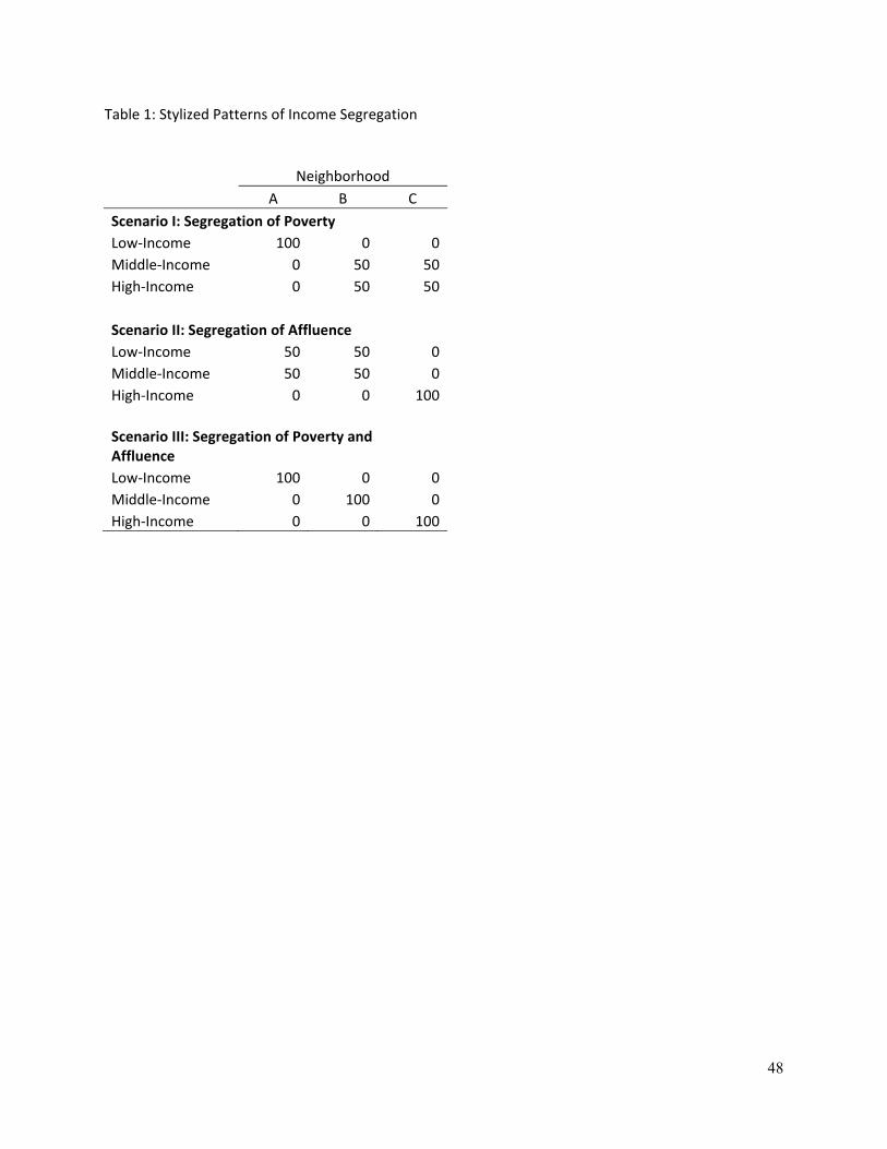
48

Table 1: Stylized Patterns of Income Segregation 

Neighborhood   A  B  CScenario I: Segregation of Poverty Low‐Income  100  0 0Middle‐Income  0  50 50High‐Income  0  50 50

Scenario II: Segregation of Affluence Low‐Income  50  50 0Middle‐Income  50  50 0High‐Income  0  0 100

Scenario III: Segregation of Poverty and Affluence Low‐Income  100  0 0Middle‐Income  0  100 0High‐Income  0  0 100 

 

Table 2: Income Inequality and Income Segregation Trends, by Race, 100 Largest Metropolitan Areas, 1970‐2000  

 

Group 1970 1980 1990 2000 Change 1970 1980 1990 2000 Change

Black 0.376 0.410 0.430 0.436 0.060 0.099 0.133 0.173 0.170 0.071(0.018) (0.017) (0.030) (0.024) (0.029) (0.036) (0.042) (0.044)

White 0.344 0.341 0.369 0.384 0.040 0.110 0.117 0.132 0.139 0.029(0.028) (0.020) (0.026) (0.025) (0.039) (0.043) (0.043) (0.046)

Black‐White Difference 0.032 0.069 0.061 0.052 0.020 ‐0.011 0.016 0.041 0.031 0.042

All Families 0.352 0.360 0.384 0.400 0.048 0.124 0.134 0.152 0.157 0.033(0.029) (0.023) (0.026) (0.025) (0.044) (0.052) (0.050) (0.051)

Income Inequality (Gini Index) Income Segregation (rank‐order H)

 Notes: Standard deviations  in parentheses.  Sample includes  100 largest metropolitan areas  (according to 2000 population).  For blacks, sample includes  61 of 100 metropolitan areas  with at least 10,000 black families  in each census  1970‐2000.

   

49

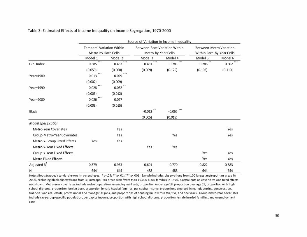
Table 3: Estimated Effects of Income Inequality on Income Segregation, 1970‐2000  

   

Gini Index 0.385 *** 0.467 *** 0.431 *** 0.783 *** 0.286 ** 0.502 ***

(0.059) (0.060) (0.069) (0.125) (0.103) (0.110)           

Year=1980 0.013 *** 0.029 ***

(0.002) (0.009)

Year=1990 0.028 *** 0.032 **

(0.003) (0.012)

Year=2000 0.026 *** 0.027

(0.003) (0.015)

Black ‐0.013 ** ‐0.065 ***           

(0.005) (0.015)           

Model Specification

     Metro‐Year Covariates Yes Yes

     Group‐Metro‐Year Covariates Yes Yes Yes

     Metro‐x‐Group Fixed Effects Yes Yes

     Metro‐x‐Year Fixed Effects Yes Yes

     Group‐x‐Year Fixed Effects Yes Yes

     Metro Fixed Effects Yes Yes

Adjusted R2 0.879 0.933 0.691 0.770 0.822 0.883           

N 644 644 488 488 644 644           

Between‐Race Variation Within Metro‐by‐Year Cells

Between‐Metro Variation Within Race‐by‐Year Cells

Source of Variation in Income Inequality

Model 1 Model 2

Notes: Bootstrapped standard errors  in parentheses.  * p<.05; ** p<.01; *** p<.001.  Sample includes  observations  from 100 largest metropolitan areas in 2000, excluding black observations from 39 metropolitan areas  with fewer than 10,000 black famil ies in 1970.  Coefficients  on covariates  and fixed effects not shown.  Metro‐year covariates include metro population, unemployment rate, proportion under age 18, proportion over age 65, proportion with high school  diploma, proportion foreign born, proportion female headed families, per capita income, proportions  emplyed in manufacturing, construction, financial  and real  estate, professional  and managerial  jobs, and proportions  of housing built within ten, five, and one years.  Group‐metro‐year covariates  include race‐group‐specific population, per capita income, proportion with high school  diploma, proportion female headed famil ies, and unemployment rate.

Model 3 Model 4 Model 5 Model 6

Temporal Variation Within Metro‐by‐Race Cells

50

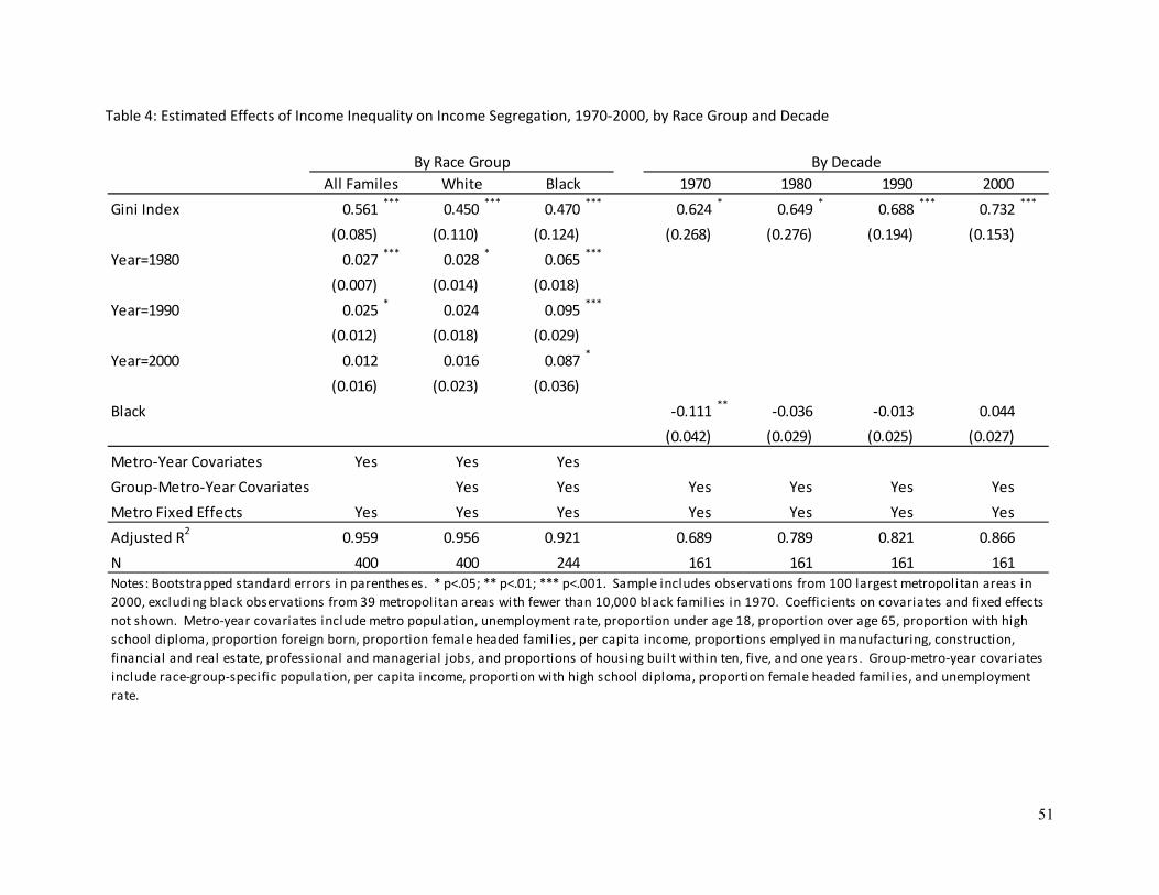
51

 

Gini Index 0.561 *** 0.450 *** 0.470 *** 0.624 * 0.649 * 0.688 *** 0.732 ***

(0.085) (0.110) (0.124)            (0.268) (0.276) (0.194) (0.153)         

Year=1980 0.027 *** 0.028 * 0.065 ***

(0.007) (0.014) (0.018)           

Year=1990 0.025 * 0.024 0.095 ***

(0.012) (0.018) (0.029)           

Year=2000 0.012 0.016 0.087 *

(0.016) (0.023) (0.036)           

Black ‐0.111 ** ‐0.036 ‐0.013 0.044           

(0.042) (0.029) (0.025) (0.027)         

Metro‐Year Covariates Yes Yes Yes

Group‐Metro‐Year Covariates Yes Yes Yes Yes Yes Yes

Metro Fixed Effects Yes Yes Yes Yes Yes Yes Yes

Adjusted R2 0.959 0.956 0.921 0.689 0.789 0.821 0.866           

N 400 400 244 161 161 161 161           

All Familes White 1970 1980 1990 2000

Notes: Bootstrapped standard errors  in parentheses.  * p<.05; ** p<.01; *** p<.001.  Sample includes  observations  from 100 largest metropolitan areas  in 2000, excluding black observations  from 39 metropolitan areas  with fewer than 10,000 black families  in 1970.  Coefficients  on covariates  and fixed effects  not shown.  Metro‐year covariates  include metro population, unemployment rate, proportion under age 18, proportion over age 65, proportion with high school  diploma, proportion foreign born, proportion female headed families, per capita income, proportions  emplyed in manufacturing, construction, financial  and real  estate, professional  and managerial  jobs, and proportions  of housing built within ten, five, and one years.  Group‐metro‐year covariates  include race‐group‐specific population, per capita income, proportion with high school  diploma, proportion female headed families, and unemployment rate.

BlackBy Race Group By Decade

Table 4: Estimated Effects of Income Inequality on Income Segregation, 1970‐2000, by Race Group and Decade  

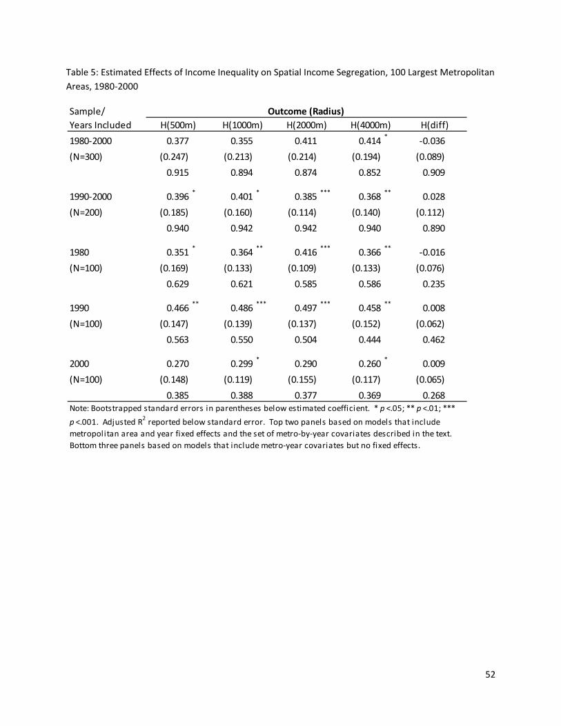
Table 5: Estimated Effects of Income Inequality on Spatial Income Segregation, 100 Largest Metropolitan Areas, 1980‐2000 

 

1980‐2000 0.377 0.355 0.411 0.414 * ‐0.036

(N=300) (0.247) (0.213) (0.214) (0.194) (0.089)

0.915 0.894 0.874 0.852 0.909

1990‐2000 0.396 * 0.401 * 0.385 *** 0.368 ** 0.028         

(N=200) (0.185) (0.160) (0.114) (0.140) (0.112)           

0.940 0.942 0.942 0.940 0.890        

1980 0.351 * 0.364 ** 0.416 *** 0.366 ** ‐0.016           

(N=100) (0.169) (0.133) (0.109) (0.133) (0.076)           

0.629 0.621 0.585 0.586 0.235     

1990 0.466 ** 0.486 *** 0.497 *** 0.458 ** 0.008           

(N=100) (0.147) (0.139) (0.137) (0.152) (0.062)           

0.563 0.550 0.504 0.444 0.462        

2000 0.270 0.299 * 0.290 0.260 * 0.009

(N=100) (0.148) (0.119) (0.155) (0.117) (0.065)

0.385 0.388 0.377 0.369 0.268Note: Bootstrapped standard errors  in parentheses  below estimated coefficient.  * p <.05; ** p <.01; *** 

p <.001.  Adjusted R2 reported below standard error.  Top two panels  based on models  that include metropolitan area and year fixed effects  and the set of metro‐by‐year covariates  described in the text.  Bottom three panels  based on models  that include metro‐year covariates  but no fixed effects.

H(500m) H(1000m) H(2000m) H(4000m) H(diff)Outcome (Radius)Sample/           

Years Included

   

52 

53 

Figure 1: Trends in Household Income Inequality, 1967‐2007 

Note: The two solid lines show the trends in the ratio of household incomes at two percentiles of the income distribution.  All trends are divided by their value in 1967 in order to put the trends on a common scale.  Source: Authors’ calculations from http://www.census.gov/hhes/www/income/histinc/p60no231_tablea3.pdf.   

0.85

0.90

0.95

1.00

1.05

1.10

1.15

1.20

1.25

1.30

Hou

seho

ld In

com

e In

equa

lity,

Rel

ativ

e to

196

7

1965 1970 1975 1980 1985 1990 1995 2000 2005 2010Year

90/50 Ratio

50/10 Ratio

Gini Index

 

Figure 2: Comparison of Stylized Income Distributions 

 

$0 $50

$100

$150

$200

$250

$300

Income (Thousands)

Income Density

$0$5

0$1

00$1

50$2

00$2

50$3

00

Inco

me

(Tho

usan

ds)

0 25th 50th 75th 100thPopulation Percentile

Inverse Cumulative Income Density

0

.25

.5

.75

1

Cum

ulat

ive

Sha

re o

f Inc

ome

0 .25 .5 .75 1Cumulative Population

Lorenz Curves

Gini Index = 0.3490/50 Ratio = 2.150/10 Ratio = 2.8

Gini Index = 0.4090/50 Ratio = 2.850/10 Ratio = 2.8

54 

Figure 3: Family Income Segregation Profile, Chicago Metropolitan Area, 2000 

0.00

0.10

0.20

0.30

0.40

0.50

Info

rmat

ion

Theo

ry In

dex,

H(p

)

$10

,000

$

15,0

00

$20

,000

$25

,000

$30

,000

$35

,000

$40

,000

$45

,000

$50

,000

$60

,000

$75

,000

$10

0,00

0

$12

5,00

0

$15

0,00

0 $

200,

000

0 20 40 60 80 100

Family Income (Dollars and Population Percentile)

Estimated Segregation at Census Category Threshold

Fitted Profile (4th-order polynomial)

 Note: Figure indicates estimated between‐tract segregation between families with incomes above and at‐or‐below each percentile of the metropolitan‐wide family income distribution.  Segregation levels at each threshold are averages of segregation levels computed from 50 random subsamples of 10,000 families from the metropolitan area.    

55 

56 

Figure 4: Trends in Family Income Inequality and Income Segregation, 1970‐2000, by Race, 100 Largest Metropolitan Areas 

0.06

0.08

0.10

0.12

0.14

0.16

0.18

Inco

me

Seg

rega

tion

(Ran

k-O

rder

HR)

0.34

0.36

0.38

0.40

0.42

0.44

0.46

Inco

me

Ineq

ualit

y (G

ini I

ndex

)

1970 1980 1990 2000 1970 1980 1990 2000 1970 1980 1990 2000

All Families White Black

InequalitySegregation

 Note: Black trends based on 61 metropolitan areas with at least 10,000 black families in each census year, 1970‐2000.

Figure 5: Trends in Family Income Inequality and Income Segregation, 1970‐2000, by Race, Small Metropolitan Areas 

0.06

0.08

0.10

0.12

0.14

0.16

0.18

Inco

me

Seg

rega

tion

(Ran

k-O

rder

HR)

0.34

0.36

0.38

0.40

0.42

0.44

0.46

Inco

me

Ineq

ualit

y (G

ini I

ndex

)

1970 1980 1990 2000 1970 1980 1990 2000 1970 1980 1990 2000

All Families White Black

InequalitySegregation

 Note: Samples for each panel of the figure include all metropolitan areas with at least 10,000 families of the respective group in each year, 1970‐2000, excluding 100 largest metropolitan areas.  Trends for all families based on 179 metropolitan areas; trends for white families based on 176 metropolitan areas; trends for black families based on 15 metropolitan areas.    

57 

Figure 6: Trends in Average Metropolitan Area Income Segregation, by Income Percentile, All Families, 100 Largest Metropolitan Areas, 1970‐2000 

0.08

0.12

0.16

0.20

0.24

0.28

Inco

me

Segr

egat

ion

(H(p

))

0 20 40 60 80 100Percentile of Metropolitan Income Distribution

1970

1980

1990

2000

1970 1980 1990 2000Year

10th

50th

90th

Percentile

 Note: Left panel of figure indicates estimated average between‐tract segregation (as measured by the information theory index, H) between families with incomes at‐or‐above and below each percentile of the metropolitan‐wide family income distribution.  Right panel shows trends for between‐tract segregation at three specific percentiles. 

   

58 

Figure 7: Trends in Average Metropolitan Area Income Segregation, by Income Percentile, White Families, 100 Largest Metropolitan Areas, 1970‐2000  

0.08

0.12

0.16

0.20

0.24

0.28

Inco

me

Segr

egat

ion

(H(p

))

0 20 40 60 80 100Percentile of Metropolitan Income Distribution

1970

1980

1990

2000

1970 1980 1990 2000Year

10th

50th

90th

Percentile

 Note: Left panel of figure indicates estimated average between‐tract segregation (as measured by the information theory index, H) between white families with incomes at‐or‐above and below each percentile of the metropolitan‐wide family income distribution.  Right panel shows trends for between‐tract segregation at three specific percentiles. 

   

59 

Figure 8: Trends in Average Metropolitan Area Income Segregation, by Income Percentile, Black Families, 61 Largest Metropolitan Areas with at least 10,000 Black Families, 1970‐2000 

0.08

0.12

0.16

0.20

0.24

0.28

Inco

me

Segr

egat

ion

(H(p

))

0 20 40 60 80 100Percentile of Metropolitan Income Distribution

1970

1980

1990

2000

1970 1980 1990 2000Year

10th

50th

90th

Percentile

 Note: Left panel of figure indicates estimated average between‐tract segregation (as measured by the information theory index, H) between black families with incomes at‐or‐above and below each percentile of the metropolitan‐wide family income distribution.  Right panel shows trends for between‐tract segregation at three specific percentiles. 

   

60 

Figure 9: Average Metropolitan Area Spatial Household Income Segregation, by Income Percentile and Local Environment Radius, 100 Largest Metropolitan Areas, 2000 

 Note: Solid lines indicate estimated average between‐tract segregation (as measured by the spatial information theory index, H, using four different local environment radii) between families with incomes above and at‐or‐below each percentile of the metropolitan‐wide family income distribution.  Dashed line indicates ratio of segregation using a 4000m radius to that using a 500m radius. 

0.35

0.40

0.45

0.50

0.55

0.60

0.65

Mac

ro/M

icro

Rat

io (H

4000

m/H

500m

)

0.00

0.04

0.08

0.12

0.16

0.20

0.24

Spat

ial I

ncom

e S

egre

gatio

n (H

(p))

0 20 40 60 80 100Percentile of Metropolitan Income Distribution

500m Radius

1000m Radius

2000m Radius

4000m Radius

H4000m/H500m

   

61 

Figure 10: Estimated Effects of Family Income Inequality on Income Segregation, by Percentile of Income Distribution and Model, 100 Largest Metropolitan Areas, 1970‐2000  

-0.5

0.0

0.5

1.0

1.5

Est

imat

ed E

ffect

5 25 50 75 95 5 25 50 75 95 5 25 50 75 95Between-Decade Model Between-Group Model Between-Metro Model

 Note: Bars indicate 95% confidence interval for estimates.  Model specifications and samples are identical to those of Model 2 (between‐decade model), Model 4 (between‐group model), and Model 6 (between‐metro model) in Table 3 above.   

62 

Figure 11: Estimated Effects of Family Income Inequality on Income Segregation, by Percentile of Income Distribution and Race, 100 Largest Metropolitan Areas, 1970‐2000  

-0.5

0.0

0.5

1.0

1.5

Est

imat

ed E

ffect

5 25 50 75 95 5 25 50 75 95 5 25 50 75 95All Families White Black

 Note: Bars indicate 95% confidence interval for estimates.  Model specifications and samples are identical to those of Columns 1‐3 of Table 4.   

63 

Figure 12: Estimated Effects of Income Inequality on Spatial Household Income Segregation, by Local Environment Radius and Percentile of Income Distribution, 100 Largest Metropolitan Areas, 1980‐2000  

-1.0

-0.5

0.0

0.5

1.0

1.5

Est

imat

ed E

ffect

5 25 50 75 95 5 25 50 75 95 5 25 50 75 95 Total Effect (H500m) Macro-Scale Effect (H4000m) Net Micro-Scale Effect

 

Note: Bars indicate 95% confidence interval for estimates.  Model specifications and samples are identical to those of Column 1 of Table 4.  Left panel shows estimates from models where outcome variable is the spatial information 

theory index   using a 500m radius and computed at the specified percentiles.  Middle panel shows estimates where outcome variable is the same, but using a 4000m radius.  Right panel shows the estimates from models 

where the outcome is the net‐micro segregation—the difference between   and  . 

 

   

64 

Appendix

Appendix Section 1: Computing Income Segregation

Practical Issues in Computing the Rank-Order Information Theory Index (

To compute from Equation (3), we need to know the function over the domain 0,1 .

In practice, however (given Census data, for example), we can compute for only a finite number of

values of , corresponding to the income category thresholds that the Census uses to report incomes. For

example, in the 2000 Census, income was reported in 16 categories (“less than $10,000,” “$10,000-

$15,000,” “$15,000-$20,000,” and so on, up to “$150,000-$200,000”, and “greater than $200,000”).

These allow us to compute at 15 distinct values of (those corresponding to 10,000 ,

15,000 ,…, 200,000 in this case). Within each census tract, the Census provides counts

(estimates, really, based on a 1-in-6 sample) of the number of families with incomes below each of these

income thresholds. For each of the thresholds, we can compute , the proportion of the population with

incomes below the threshold and , the information theory index of segregation between those below

the thresholds and those at or above the threshold. Following Reardon et al. (2006), we then approximate

the function over the range 0,1 by fitting an -th order polynomial to the values, weighting each

point by the square of :

, ~ 0,

(A1)

We use a fourth-order polynomial here, but our results are insensitive to the choice of any higher-order

polynomial. If is the estimated -th coefficient from this model, then Reardon et al. (2006) show that

equation (3) will evaluate to

12

22

21

2,

(A2)

where !! !

denotes the binomial coefficient (the number of distinct combinations of

65 

elements from a set of size ). While this looks messy, in practice, the procedure is straightforward: 1)

for each income threshold reported by the Census, we compute , the proportion of the relevant

population below threshold ; 2) we compute , the information theory index of segregation

between those above and below the income threshold , for each threshold ; 3) we fit a polynomial

regression model through the points , ; and 4) we use the estimated coefficients from the model

to compute an estimate of from Equation (A2).

Once we have estimated the function from Equation (A1), we can also compute estimated

values of segregation at any desired threshold. Suppose, for example, we wish to estimate the segregation

between families in the top 10 percent of the income distribution and all others. Even if there is not an

income threshold in the Census data that corresponds exactly to the 90th percentile, we can estimate . 9

from the fitted polynomial (Equation 4). For example, even though there is no income threshold in

Chicago that corresponds exactly to the 90th income percentile, we can compute the estimated value of

. 9 0.370 from the estimated parameters of the fitted profile in Figure 3. This will enable us

to compute and compare the segregation levels of well-defined income groups even when the Census

does not provide the exact information needed.

Correcting Small Sample Bias in Income Segregation Measures

One complication with comparing income segregation levels across metropolitan areas and racial

groups is that evenness measures of income segregation are biased upwards in small populations

(specifically, when the population is relatively small compared to the number of tracts). This bias results

from the fact that income segregation measures (including the rank-order information theory index) are

generally ratios of average within-unit (e.g., tracts) income variation to total population income variation.

When the number of households in a unit is small (either because the population is small or because of

sampling), estimates of within-unit variation will be biased downwards. The bias can be substantial.

When we take a random sample of 10,000 households from a metropolitan area and compare income

66 

segregation among the sample to income segregation among the total population, the sample estimates are

considerably higher. Given that Census family income data are based on 1-in-6 samples, this has

implications for comparing income segregation across metropolitan areas, years, and groups that vary in

population size.

To ensure that our comparisons of the levels of segregation among metropolitan areas, race

groups, and decades are not biased by differences in population size, we adjust the estimated segregation

levels for population size. For each of the 644 cases in our analysis, we draw 50 random samples

(without replacement) of 10,000 families of the specified racial group (or from the total population) and

compute HR from each sample. The mean of these 50 estimates provides a population-size-adjusted

estimate of income segregation for each group-metro-year case. This procedure eliminates bias due to

different population sizes, by ensuring that each of the estimates of HR are based on the same size sample.

The resulting estimates are comparable across race groups, metropolitan areas, and years, regardless of

population size.

Appendix Section 2: Data and Sample

Data Comparability Issues

Metropolitan boundaries and definitions: Metropolitan boundaries change over time. We use consistent

metropolitan area definitions across census years to ensure comparability of the results over time. We use

the OMB 2003 metropolitan area definitions, the first definitions based on the 2000 census.

Census confidentiality procedures: The Census employs certain measures to ensure confidentiality that

affect the reporting of race-specific income distributions. More specifically, the Census suppresses data

within certain geographic units when they determine that the population numbers for certain groups are

small enough to threaten the privacy rights of individuals or families. For instance, if there are only a

handful of black families in a census tract, the Census would not release the income data for black

families in that tract because it may be possible to identify individual families. In 1980 the Census also

employed complimentary suppression, which can lead to the suppression of other groups besides the

67 

small sub-group to avoid inferences through subtraction. We do not adjust our analyses for suppression,

but because we only include in our race-specific analyses metropolitan areas with greater than 10,000

families in that race group, the problem is minimized.

Income: Total income is defined by the Census as the sum of the amounts reported separately for wage or

salary income; net self-employment income; interest, dividends, or net rental or royalty income or income

from estates and trusts; social security or railroad retirement income; Supplemental Security Income

(SSI); public assistance or welfare payments; retirement, survivor, or disability pensions; and all other

income.

We use family income data from the 1970-2000 Censuses. We obtain tract-level family income

data by race for 1970, 1980, and 2000 from the Geolytics Neighborhood Change Database CDs

(GeoLytics, 2004) as well as the 1990 data from the National Historical Geographic Information System’s

online data extract system (Minnesota Population Center, 2004). This was necessary because family

income by race was not available in the STF3 files in 1990, the files available in the Geolytics CDs.

Instead, the 1990 family income by race was in the STF4a files.

The census reports income for families and households. We use family income because the data

is available by race for all four census years. Families are residential units that include two or more

people related by blood or marriage. Households are all residential units, including those that contain one

person. Thus, family income only includes those related by blood or marriage whereas household income

includes the incomes of all people living in a household. In compiling statistics on family income, the

incomes of all members 15 years old and over related to the householder are summed and treated as a

single amount. Although family income is generally higher on average than household income because

many households only contain one person, the use of household or family income yields similar results in

the regression analyses.

The Census also changes the number of income categories used in each decennial Census. For

the total population there are 15 income bins in 1970, 17 in 1980, 25 in 1990, and 16 in 2000. The

income-by-race bins are the same except for in 1980 when there are only 9 income bins by race. Our

68 

approach to measuring income segregation is insensitive to these differences.

Gini Index: The Gini index is computed from Census data using a procedure described in detail in Nielsen

and Alderson (1997).

Data Sources for, and Construction of, Covariates

Total Population (by race): 1970-2000 obtained from National Historical Geographic Information

System (NHGIS).

Unemployment (by race): 1970 obtained from NHGIS; 1980-2000 obtained from Geolytics. We

collapsed unemployment by gender and then calculate the percent of the population that is unemployed.

This measure includes persons 16 years of age and older in the civilian employment force who are not

employed.

Age: 1970 obtained from NHGIS; 1980-2000 obtained from Geolytics. We calculate the percent of the

population that is less than 18 and the percent of the population older than 65. In 1970, the under-18

category is actually under-19.

Education (by race): 1970-2000 obtained from NHGIS. We calculate the percent of the population with

at least a high school degree for the population 25 years and older.

Per Capita Income (by race): 1970-2000 obtained from NHGIS. In 1970 there was no specific variable

for per capita income so we constructed the measure using the aggregate individual income variable.

Foreign born: 1970-2000 obtained from Geolytics. We calculate the percent of the population that was

born outside of the United States.

Occupational industries: 1970-1990 obtained from NHGIS; 2000 obtained from Geolytics. We calculate

the percent of the population that is employed in the following occupational industries: Manufacturing,

Construction, FIRE (finance, insurance, and real estate), and Professional/Managerial (information, FIRE,

education, health, other professional, and public administration). This measure includes persons 16 years

of age and older in the civilian employment force.

Family structure (by race): 1970 obtained from NHGIS; 1980-2000 obtained from Geolytics. We

69 

calculate the percent of families that are headed by females. We also calculate the total number of

families.

Residential mobility: 1970-2000 obtained from Geolytics. We calculate the percent of the population that

resides in the same house as they did 5 years before as well as the percent of the population that resides in

a different house in the same county. These measures includes persons 5 years of age and older.

New housing construction: 1970 obtained from NHGIS; 1980-2000 obtained from Geolytics. We

calculate the percent of housing (occupied + vacant) that was built 10, 5, and 1 year before the census

year.

   

70 

71 

Appendix Section 3: Appendix Tables 

 Table A1: Trends in Family Income Segregation, by Race and Income Percentile, 100 Largest Metropolitan Areas, 1970‐2000  

1970 1980 1990 2000 ChangeBlack

5th  0.101 0.132 0.188 0.192 0.09110th 0.095 0.125 0.177 0.176 0.08125th 0.091 0.121 0.163 0.156 0.06550th 0.097 0.128 0.162 0.158 0.06175th 0.102 0.139 0.177 0.176 0.07490th 0.127 0.171 0.228 0.230 0.10395th 0.145 0.192 0.260 0.264 0.119

White5th  0.117 0.145 0.163 0.173 0.05610th 0.104 0.124 0.139 0.148 0.04425th 0.093 0.101 0.111 0.118 0.02550th 0.100 0.107 0.118 0.126 0.02675th 0.119 0.123 0.144 0.151 0.03290th 0.178 0.175 0.204 0.207 0.02995th 0.216 0.210 0.242 0.241 0.025

All 5th  0.134 0.180 0.208 0.203 0.06910th 0.122 0.156 0.179 0.178 0.05625th 0.112 0.124 0.140 0.144 0.03250th 0.114 0.122 0.136 0.143 0.02975th 0.128 0.134 0.156 0.163 0.03590th 0.184 0.187 0.213 0.215 0.03195th 0.221 0.223 0.250 0.247 0.026

YearGroup and Percentile

Notes: Segregation measures  indicate segregation (H ) of families  with incomes  above the specified income percentile from those with incomes  below the percentile.  Sample Includes  100 largest metropolitan areas  (according to 2000 population).  For Blacks, sample includes  61 of 100 metropolitan areas  with at least 10,000 Black families in each census  1970‐2000. 

  

Table A2: Estimated Effects of Income Inequality on Income Segregation at Various Percentiles of Income Distribution, 100 Largest Metropolitan Areas, Various Specifications, 1970‐2000  

 

Model Model 2 0.076 0.138 0.292 *** 0.474 *** 0.639 *** 0.778 *** 0.837 ***(N=644) (0.124) (0.091) (0.051) (0.057) (0.069) (0.108) (0.130)

Model 4 0.486 * 0.626 *** 0.782 *** 0.719 *** 0.849 *** 1.074 *** 1.156 ***(N=488) (0.239) (0.190) (0.166) (0.120) (0.123) (0.132) (0.147)

Model 6 0.133 0.235 0.400 ** 0.484 *** 0.631 *** 0.785 *** 0.840 ***(N=644) (0.135) (0.115) (0.124) (0.094) (0.085) (0.099) (0.129)

All Families 0.155 0.244 0.387 ** 0.550 ** 0.789 *** 0.811 *** 0.756 ***(N=400) (0.181) (0.158) (0.142) (0.169) (0.084) (0.133) (0.211)

White 0.110 0.164 0.273 ** 0.462 *** 0.661 *** 0.611 *** 0.527 *(N=400) (0.116) (0.098) (0.100) (0.118) (0.110) (0.141) (0.229)

Black 0.259 0.202 0.263 0.474 *** 0.565 *** 0.962 *** 1.250 ***(N=244) (0.276) (0.207) (0.141) (0.106) (0.107) (0.166) (0.194)Notes: Coefficients  are estimated effects  of income inequality on income segregation at specified percentile of income distribution.  Bootstrapped standard errors  in parentheses.  * p<.05; ** p<.01; *** p<.001.  Estimates  from Models  2, 4, and 6 use sample and corrresponding model  specifications  from table 3 above.  Estimates  for all  families  use sample of 100 largest metropolitan areas  and specification from Table 4 above; estimates  for white and black families  use sample of 100 largest metropolitan areas  with at least 10,000 families  of specified group (100 metropolitan areas for white models; 61 metropolitan areas  for black models) and use specification from Table 4 above.      

5th  10th  25th  50th  75th  90th  95th Percentile of Income Distribution

  

72