Embed Size (px)
Citation preview

Income Inequality and Macroeconomic Volatility: AnEmpirical Investigation
Richard Breena and Cecilia García-Peñalosab
14 July 1999
Abstract:Recently, there has been a resurgence in the interest in the determinants of incomeinequality across countries. This paper adds to this literature by examining the role of onefurther explanatory variable: macroeconomic volatility. Using a cross-section ofdeveloped and developing countries, we regress income inequality on volatility, definedas the standard deviation of the rate of output growth. We find that greater volatilityincreases the Gini coefficient and the income share of the top quintile, while it reducesthe share of the other quintiles. The other variable that seems to play an important role isrelative labour productivity, supporting previous findings.
Key words: income inequality, output volatility, cross-country regressions.
JEL Classification numbers: I30, O15.
a European University Institute, Badia Fiesolana, San Domenico di Fiesole, Florence, Italy, and Queen’s
University, Belfast BT7 1NN, UK.b Nuffield College and GREQAM,. Corresponding author: Nuffield College, Oxford, OX1 1NF, UK ph: 44-
1865-278656, fax: 44-1865-278621, email: [email protected].
Ackowledgements: We would like to thank Tony Atkinson, Steve Redding, Jon Temple, and seminar participantsat the University of Zurich.

2
1. Introduction
In recent years, inequality in earnings and income has been the focus of attention as both
the explanands and the explanandum of inquiry. On the one hand, there is a growing
literature concerned with the impact of inequality on economic growth (see, for example,
Perotti 1996). On the other, there has been a revival of interest in the factors shaping the
distributions of earnings and income. This has taken the form of studies of the evolution
over time of inequality within a country, discussed, for example, by Atkinson (1996,
1997) and Gottschalk and Smeeding (1997), and of analyses seeking to explain cross-
national variation in income inequality, such as Bourguignon and Morrissson (1998) and
Li, Squire and Zou (1998). It is to this latter strand that the present paper contributes.
The main issue that we address is whether macroeconomic volatility plays a role
in determining a country’s degree of income inequality. There are two reasons for asking
this question. First, Ramey and Ramey (1995) have found that higher volatility of the rate
of output growth is associated with a lower average growth rate. Their results raise the
question of whether volatility also affects other macroeconomic variables. Second,
Hausmann and Gavin (1996) have shown that Latin American economies are both much
more volatile and much more unequal than industrial economies, and that in fact
volatility of the level of GDP is positively correlated with inequality.
We explore this idea further, and in particular we compare the role of volatility in
determining inequality with that played by other factors previously found to have a
significant effect on inequality, such as macroeconomic dualism, financial development
and civil liberties. Following Ramey and Ramey (1995), we use the standard deviation of
3
the rate of growth of GDP over a 30-year period as our measure of macroeconomic
volatility. Using data for a cross-section of countries over the period 1960-90, we find
that volatility has a positive effect on income inequality, and that this relationship is
robust to controls for a number of other factors that the literature suggests affect
inequality. Furthermore, we show that the effect of high volatility is to increase the share
of income of the highest quintile at the expense of (mainly) those in the second and third
quintiles.
Our results are robust to the inclusion of the explanatory variables used in
previous work, such as output levels, educational attainment, relative labour productivity,
and civil liberties, among others. We find that of the variables previously found to
explain inequality only relative labour productivity and the share of labour employed in
agriculture have a consistently significant effect.
The organization of the paper is as follows. Section 2 describes existing
hypotheses about the determinants of income inequality. Section 3 starts with a
description of our dataset, which comprises a cross-section of 80 developed and
developing countries. We then present our empirical results. Our basic results are
extended to include other explanatory variables. We also examine a smaller dataset that
allows us to control for initial inequality, and test for alternative measures of volatility. In
section 4 we consider a possible explanation for our findings. Section 5 concludes.

4
2. The Determinants of Income Inequality Across Countries
Over the past fifty years, several hypotheses have been postulated to explain differences
in the distribution of income among countries. The first of these was Kuznets’ argument
(Kuznets, 1955 and 1963) that inequality increases in the early stages of development,
but falls as industrialization goes on, as a result of the interplay between the rural-urban
income differential and the share of the population in one or the other sector. This
hypothesis would then imply that, at a particular point in time, we should observe an
inverted-U shaped relationship between a country’s level of development –proxied by per
capita income- and its degree of inequality.
The Kuznets hypothesis has been subject to close scrutiny both from a theoretical
and an empirical point of view. Anand and Kanbur (1993a,b) maintain that there are two
major problems with it. On the empirical side, Anand and Kanbur (1993b) find no
support for the inverted-U relationship on a cross-section of countries. They then argue
(see Anand and Kanbur, 1993a) that this may be due to a theoretical misspecification. In
particular, it is important to allow sectoral means and sectoral inequalities to change over
time, and once we do this the evolution of inequality may follow many different patterns.
Bourguignon and Morrisson (1998) argue that the Kuznets process is too complex
to be simply proxied by GDP per capita, and that both the rural-urban income differential
and migration between the two sectors are endogenously determined. Under perfectly
competitive labour markets the distribution of income in a country will be determined by
factor endowments and the distribution of factor ownership. However, labour markets are
seldom competitive and a more appropriate approach is to think of a dual economy
model. In this framework, an indicator of the imperfection of the labour market- i.e. a

5
measure of the extent of dualism in the economy- should help explain differences in the
distribution of income. They propose the use of the relative labour productivity (RLP)
between agriculture and the rest of the economy as a measure of dualism, and find, in a
cross-section of developing countries, that the lower is RLP in agriculture the more
unequal the economy. Measures of factor endowments, such as cultivable land per capita,
seem to have no robust effect.
Other macroeconomic variables have been found to be associated with the
distribution of income. In their study of the determinants of inequality, Li, Squire and
Zou (1998) examine the impact of four variables: initial secondary schooling, civil
liberties, financial development and the Gini coefficient of the distribution of land. They
find that all these variables have a significant effect on the Gini coefficient: higher level
of schooling, civil freedom and financial development reduce inequality, while the more
unequal the distribution of land, the more unequal that of income. Bourguignon and
Morrisson (1990) point to the role of trade liberalisation in increasing inequality. In
particular, they find that trade protection plays a significant role. Lastly, Alesina and
Perotti (1996) find a positive correlation between socio-political instability and
inequality, although they argue that causation runs from the distribution of income to
instability.
These papers provide us with a set of ideas about the possible determinants of
income inequality. Our analysis of the influence of volatility on inequality must also test
the robustness of its effect to the inclusion of these variables.

6
3. The influence of volatility on the distribution of income
3.1 The data
Our analysis of cross-country differences in inequality is limited by the availability of
data on the distribution of income. We draw on the Deininger and Squire (1996) dataset,
which consists of a large compilation of country data for almost 200 economies. Each
observation relates to a particular country in a particular year and includes the Gini
coefficient of income and, for some cases, quintile shares. In general, there is no
consistency in the surveys either across countries or over time within a country. Surveys
differ in their coverage (national, rural and urban), income unit (household or personal
income), the source of the calculations (income or expenditure) and whether it is gross or
net income that they report. Following the arguments of Atkinson and Brandolini (1999),
we do not consider only the “high quality” subset of the Deininger-Squire data set.
Instead, we select all the observations that were obtained from surveys of national
coverage (see the appendix for a more detailed description of the data).
The data within our subset still presents a problem because the income units, the
source of income and whether it is measured net or gross of tax all differ among the
observations. One means of dealing with these differences is to “adjust” the data by
calculating the difference between, say, the average Gini coefficient of household and the
average Gini coefficient of personal income, and then adding it to those observations that
report household income (Perotti (1996) and Li, Squire and Zou (1998) adjust the data in
this way). The drawback of this approach is that the adjustment coefficients depend
crucially on the sample chosen. Instead, we will follow Bourguignon and Morrisson
7
(1998) and include dummy variables in our regression equations in order to control for
these differences.
To obtain a measure of volatility we calculate the annual rate of growth of real per
capita GDP over the period 1960 to 1990. Output volatility is then defined as the standard
deviation of the annual growth rate, as done by Ramey and Ramey (1995). This is in
contrast with Hausmann and Gavin (1996), who define macroeconomic volatility as the
standard deviation of the level of GDP per capita. The problem with using the latter
measure of volatility is that an economy which is growing at a high but constant rate will
nevertheless display high volatility. Given the variety of growth patterns observed within
our sample, we prefer a measure which is not sensitive to growth in this way.
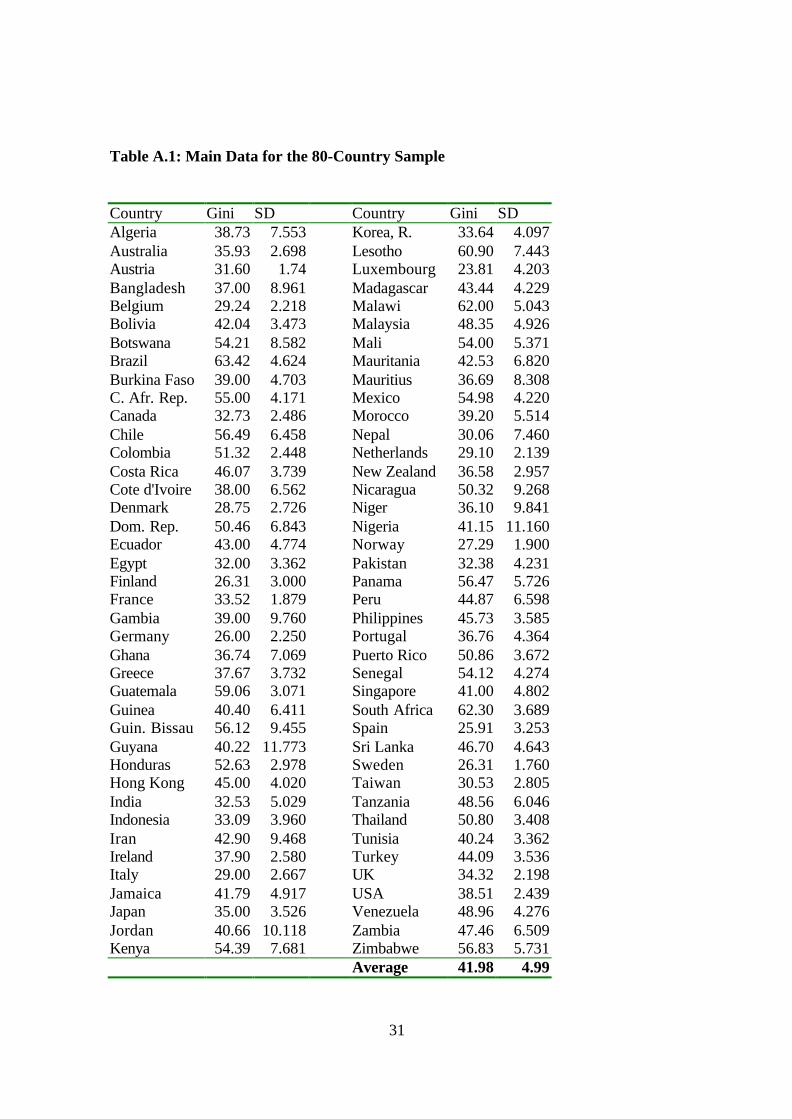
There are 80 countries for which we have data on inequality and GDP for the
period. Our sample incorporates 22 developed countries, 17 Latin- and Central-
American, 5 New-Industrialising countries, 11 other Asian countries, and 25 African
economies. Table A.1 in the appendix gives the list of countries.
3.2 Basic results
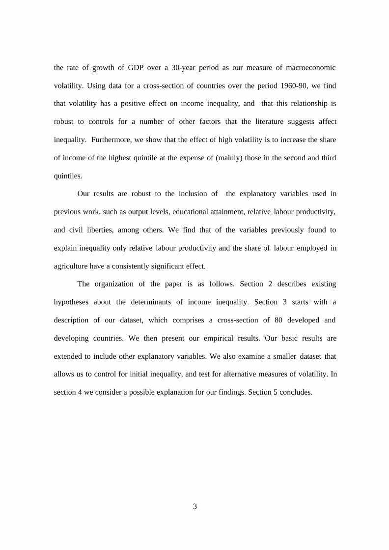
Figure 1 presents a scatter plot of the Gini coefficient against output volatility for the 80-
country sample. A simple regression of the Gini coefficient, denoted iG , on volatility,
iSD , and its square yields the following equation
(0.117) (1.505) (3.963)
590.0278.8879.18)( 2iii SDSDGE −+=
( 224.02 =R , standard errors in parenthesis). This simple regression equation is capable
of explaining a substantial fraction of the variation in inequality across countries.
Countries where output is very volatile are more unequal, except for very high levels of

8
volatility. The partial derivative of G with respect to SD is positive for all values of the
latter less than 7. For greater volatility, the relationship seems to break down. In fact,
when we divide our sample into two subsets, we find that for the 16 observations with a
value of SD above 7 there is no significant relationship between volatility and inequality.
Figure 1 and Table 1 around here
Table 1 reports 6 regressions run on the Gini coefficient of the distribution of income
in 1990. All equations in table 1, as in the rest of the paper, are OLS estimations with
heteroschedasticity consistent errors. We included three dummy variables (for net
income, for household income, for expenditure measures) in order to control for
differences in the measurement of inequality. Of these only the dummy for net income
has a significant coefficient. Our basic equation, column 1, is then augmented to test for
the robustness of the effect of volatility to the inclusion of two standard variables: the
Kuznets effect and education. A simple regression of the Gini coefficient on the level of
output and its square yields the familiar bell-shaped relationship between the level of
income and inequality. This relationship weakens once we include a measure of human
capital (not reported), and entirely disappears when we control for volatility. Column 3
reports this result when we use as a measure of human capital the percentage of
individuals in the total population who have attained secondary schooling (Sec85).1
Instead of a Kuznets effect, we find that the level of income has a negative and
significant effect on the Gini coefficient, indicating that more developed countries have
more egalitarian distributions –even before taxes.
1 The volatility effect is robust to the use of other measures of education.
9
The next two columns include other variables linked to the level of economic
development. The first one is the rate of output growth. As already mentioned, Ramey
and Ramey (1995) find that greater volatility is associated with lower growth. If growth
then affects inequality through some sort of Kuznets mechanism, it could be the case that
the coefficient on volatility is capturing an indirect relationship going from volatility to
growth and from growth to inequality. Column 5 indicates that, although countries that
have grown faster have, at the end of the period, a lower level of inequality, the effect of
volatility on the income distribution is not mediated by the rate of growth.
The last regression equation in table 1 includes investment (as a share of GDP,
averaged over the period 1960-89) as an explanatory variable. Physical capital
accumulation has no impact on the Gini coefficient, in line with the results obtained by
Li, Squire and Zou (1998, table 8). Educational attainment reduces inequality in all our
specifications. Note that this effect is not made insignificant by the presence of LnGDP,
indicating that both the level of income and the level of education affect distribution.
3.3. Other influences on inequality
The relationship between inequality and volatility reported in Table 1 could be caused by
a common factor that affects both variables. In particular, there are differences between
regions of the world – in policies, in institutions or in the structure of production– which
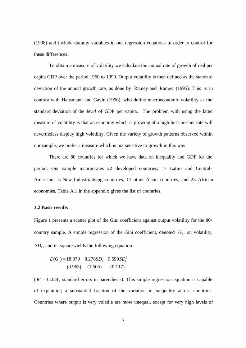
affect both inequality and volatility. Figure 2 depicts the relationship between volatility
and inequality in the various geographical regions. Countries have been divided into five
groups: Africa, Latin America, the New Industrializing Countries, other Asian
economies, and OECD economies. Each point in the graph represents the (unweighted)

10
average volatility and average inequality for each group. Those regions with high levels
of volatility also tend to exhibit high levels of inequality.
Figure 2 and Table 2 around here
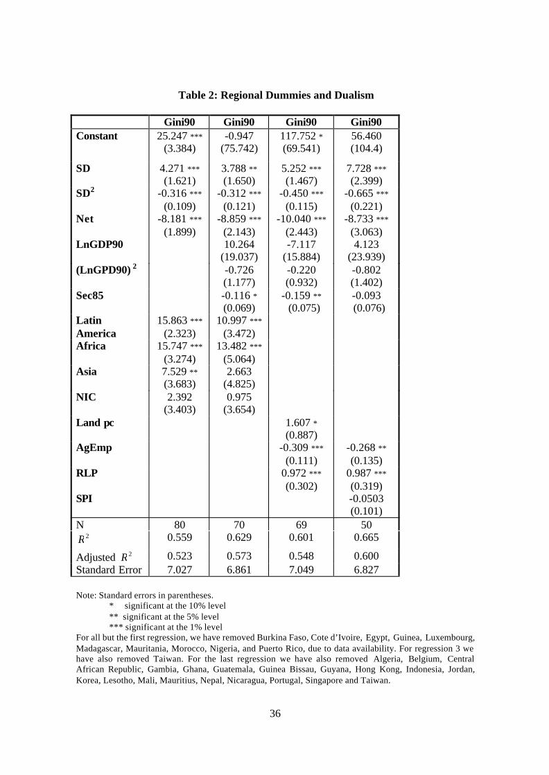
Column 1 of Table 2 reports estimates obtained when we include regional dummies
in our basic regression equation for the Gini coefficient. Dummies for Latin America,
Asia and Africa have positive and statistically significant coefficients, but, although their
presence reduces the impact of volatility on inequality, these effects nevertheless remain
substantively and statistically significant. Volatility seems to be able to explain
differences in inequality both across regions of the world and within those regions. The
next column introduces regional dummies together with measures of the level of
education and of output level. Our results are similar to those in table 1.
The impact of output volatility on inequality is not only statistically significant,
but also economically significant. Consider the second equation in table 2. For the US, an
increase in volatility of one standard deviation of the distribution of volatility in our
sample –up to the level of Ecuador and Malaysia- would result in an increase in the Gini
coefficient of 6.4 points, which represents 64% of the standard deviation of Gini90 in our
sample. An increase in volatility up to the level of Chile’s (i.e. from 2.44 to 6.46) would
raise the Gini coefficient in the US by one standard deviation. For Kenya, a reduction in
volatility to the level experienced by the US –that is, of about two standard deviations-
would reduce its Gini coefficient by 11 points, which is more than one standard deviation
of Gini90.
The rest of table 2 and table 3 examine whether introducing other variables
previously found to affect inequality reduces the impact of macroeconomic volatility.

11
Columns 3 and 4 of table 2 consider the effect of both the agricultural structure of an
economy and the degree of dualism. The regression equations are similar to those in
Bourguignon and Morrisson (1998),2 except that we also include our measure of
volatility and its square. The results are similar to those reported in their paper. GDP per
capita and education have a weak effect, sensitive to which other variables are included.
We find that cultivable land per capita has a positive impact on inequality, in contrast
with the negative (though often insignificant) coefficient obtained by Bourguignon and
Morrisson. In our sample, the coefficient on this variable is driven by one observation,
Australia, and in fact the coefficient on land per capita becomes insignificant once it is
excluded from the sample. The share of agriculture in total employment, AgEmp, has a
negative and significant effect, while relative labour productivity has a positive and
significant effect, indicating that the greater the extent of macroeconomic dualism, the
more unequally income is distributed. Lastly, we also included in our regression equation
a measure of socio-political instability (SPI), which proves to have no impact.
Table 3 around here
The regression equations reported in Table 3 include further variables based on
the analysis of Li, Squire and Zou (1998): schooling measured as mean years of
secondary schooling of the population in 1960, and denoted MYSch; an index of civil
liberties, CIVLIB, with 1 assigned to countries with the largest degree of civil liberties
and 7 to those with the smallest; and financial development, FNDP, measured by the ratio
2 We have used the share of agriculture in employment rather than in output as both in the results of Bourguignon andMorrison and in ours, the latter generally had no significant effect. We have not included two of their variables: mineralresources -which they found never to have a significant effect- and the share of small and medium farmers –as we onlyfound data on this for a small number of countries.

12
of either M1 or liquid liabilities to GDP averaged over 1960-1989.3 We do not include
the Gini coefficient for land, as we have only found data for a small number of countries.
The first two columns in Table 3 report an equation similar to that estimated by
Li, Squire and Zou (1998), except that we have not included the Gini coefficient of land
amongst the regressors. Secondary schooling in 1960 has no significant effect, while the
other two variables have the expected effect on inequality: fewer civil liberties –a higher
value of CIVLIB- increase inequality, and more financial development reduces it. When
we replace MYSch with Sec85, that is a measure of human capital at a point in time
closer to our measure of inequality, all three variables have a significant effect (not
reported). The next four columns include volatility as a regressor. Its effect seems robust
and the coefficients are similar to those obtained in previous specifications.
The last two columns of table 3 also allow us to compare the hypotheses proposed
by, on the one hand, Bourguignon and Morrisson (1998) and, on the other, Li, Squire and
Zou (1998). The coefficients on civil liberties and financial development are strongly
affected by the presence of other explanatory variables. In particular, adding the level of
GDP per capita as a regressor renders the impact of these two variables insignificant.4
The effect of dualism and employment in agriculture seem, however, robust.
We ran further regressions to test for other of the possible effects discussed in
section 2. One of them is the impact of openness on the link between volatility and
inequality. We do this by adding, to our basic inequality equation, the average of the ratio
of imports plus exports to GDP over the 1960-89 period. The openness measure had no
3 See the data appendix for the sources and exact definitions.
4 In their sensitivity analysis, Li, Squire and Zou (1998, table 9) include as a regressor “initial” GDP –i.e. GDP per capita in1960- and find that the coeeficients of the variables of interest remain significant. We use current GDP, that is the level ofoutput in 1990.
13
significant effect and the coefficients on volatility were unaffected by its inclusion. We
obtained identical results when we substituted a measure of the average ratio of exports to
GDP and when we used the change in openness between 1960 and 1990.
In order to understand better the way in which volatility affects inequality we
examine the impact it has on the income shares of various groups. Table 4 reports
regressions of the shares of the five quintiles on volatility and other variables (data is
available for only a subset of our sample). Greater volatility increases the income share of
the top 20% of the population, and reduces that of all other quintiles. The effect is
particularly strong on the shares of the 5th, 3rd and 2nd quintiles, indicating that volatility
results in redistribution from the middle class towards the wealthiest households. The
weak impact of volatility on the 4th quintile is probably due to the fact that we are not
using an appropriate division of income groups, as volatility may increase the income
share of the richest in this group (those close to the top 20%) and reduce that of
individuals close to the 3rd quintile.
Table 4 around here
It is hard to distinguish the effect of education and the level of income. In the
particular formulation reported in table 4, both a greater level of education and of income
reduce the share of the top quintile. However, when the square of LnGDP90 is added to
the regression equation, the coefficients on all three terms become insignificant. Dualism
has a positive impact on the top quintile, a negative one on the rest, in accordance with
the results obtained by Bourguignon and Morrisson (1998). We also included our
measures of financial development, which were significant only in the absence of
14
LnGDP. Other variables considered – such as civil liberties and land per capita – proved
to have no effect on the quintile shares.
3.4. The role of initial inequality
In this subsection we report the results of running regressions, similar to those already
described, but in which we control for the initial level of inequality. There are two
reasons for doing this. First, we lack measures of some of the factors that influence
inequality – such as institutional or social factors that differ between countries. To the
extent that these factors change only slowly over time, they will also be a determinant of
initial inequality and, consequently, we can use initial inequality as a proxy for at least
some of them. Secondly, having two observations from each country provides a way of
controlling, to some extent, for possible country-specific discrepancies in the way in
which the data on the distribution of income were collected.
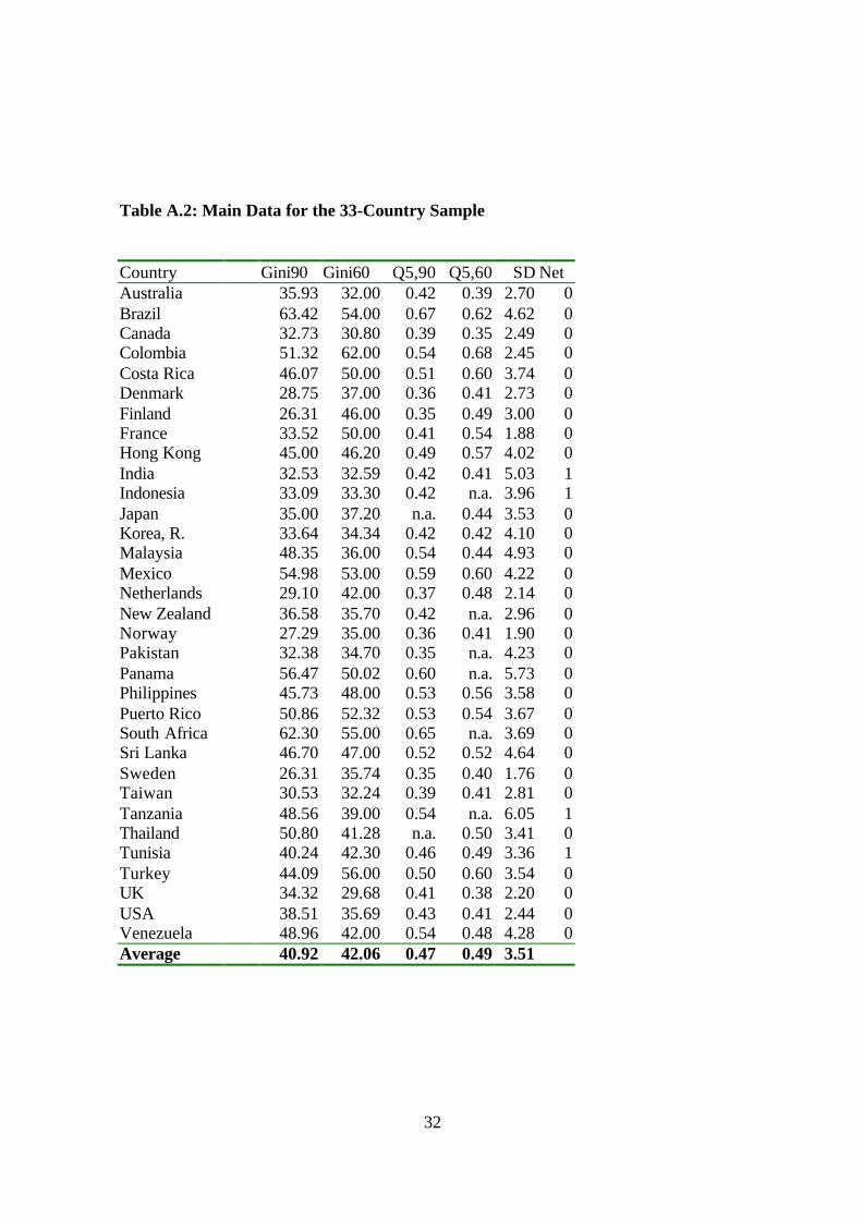
Our data set is substantially reduced when we incorporate an observation on
initial inequality (i.e around 1960). Further more, there are several countries for which an
observation exists for both periods, but income is measured in different ways. We
therefore consider only those countries in our sample for which we have two consistent
observations. This reduces the sample dramatically to 33 countries. Although small, our
sample is a representative set in the sense that it incorporates countries from different
regions (see table A.2, in the appendix).
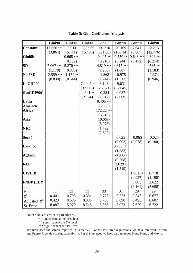
Table 5 reports the estimated regression equations for the Gini coefficient. The
first column presents the basic equation: volatility has the expected positive coefficient
and is highly significant. We have dropped the squared-volatility term and the dummy
variable for net income, and replaced them with the interaction between volatility and net

15
income.5 In this smaller sample, the coefficient on the square of volatility becomes
insignificant, the reason being that we have lost all the observations with very high levels
of volatility (Algeria, Bangladesh, Botswana, Gambia, Ghana, Guinea Bissau, Guyana,
Iran, Jordan, Kenya, Lesotho, Mauritius, Nepal, Nicaragua, Niger, Nigeria). The
interactive term provided a better fit than a model with a dummy variable for net.
Table 5 around here
In general, the results that we obtained with the larger sample are reproduced by
the smaller one. The effect of volatility on inequality is not eroded by controlling for
initial inequality, as its coefficient remains positive and significant. In Column 3 of the
table we estimate a simple Kuznets curve and we obtain the expected inverse U-shaped
relationship. However, once volatility and regional dummies are included as regressors
(column 4) the coefficients on the two income variables become insignificant. The last
three columns test for the effect of, on the one hand, dualism and, on the other, financial
development and civil liberties. Two things are worth noting. First, that in all the
specifications the coefficient on volatility remains positive, statistically significant, and
economically important (an increase in volatility of one standard deviation, implies a rise
in the Gini coefficient of half its standard deviation in the smaller sample). Second, that
once we include initial inequality and volatility the coefficients on most other variables
become insignificant.
Table 6 reports regression equations for quintile shares, which again are similar to
those obtained with the larger sample, with volatility increasing the share of the top
quintile and reducing that of the second and third. Given our previous results, it is
5 As in the larger sample, the dummies for personal income and expenditure-based estimates prove to have insignificant
coefficients.

16
surprising to find hardly any effect of relative labour productivity. This is probably due to
the fact that, since almost half of the countries in the sample are developed economies,
there is not much variability in this variable (the standard deviation of this variable drops
dramatically, from 3.9 in the large sample to 1.6 in the small one).
Table 6 around here
We ran the small sample models (i.e. those that include initial inequality) on a
different data set consisting of only the ‘high quality’ observations in the Deininger and
Squire dataset (these results are available on request from the authors). We found that the
coefficients of most variables were generally not robust to either the specification or the
data set used. By contrast, the volatility effect was consistently strong and significant.
3.5. Alternative measures of volatility
Using the standard deviation of growth rates as a measure of volatility is the approach
generally followed by the literature on this topic. It may, however, be an unsatisfactory
proxy (see Pritchett, 1998). Consider, for instance, two countries with the following
growth patterns: country A has annual growth rates of 4%, 2%, 4%, 2%, 4%, and 2%,
while country B has 4%, 4%, 4%, 2%, 2%, and 2%. They will have the same average rate
of growth and standard deviation (3% and 1.095, respectively) but clearly correspond to
different levels of volatility. A possible way of dealing with this problem is to define
higher order measures, such as the standard deviation of the first differences of the annual
growth rates. This alternative measure of volatility yields a value of 2.19 for the first
series, and of 0.89 for the second one, indicating that A is more volatile than B.
We follow this approach and calculate the standard deviation of changes in the
annual rate of growth, denoted SD(∆g). The correlation between this measure and the

17
standard deviation of the annual rate of growth is 0.95. This seems to indicate that, in
general, we are not dealing with processes such as that in country B. When we re-
estimate our basic regression equation using this new measure of volatility, we obtain the
following equation:
(2.119) (0.055) (0.973) (3.403)
1787.6)(315.0)(395.6102.21)( 2 NetgSDgSDGE iii −∆−∆+=
( 278.02 =R , SE=8.802, standard errors in parenthesis). The results are very similar to
those reported in table 1, and the fit of the regression equation is only slightly worse than
when we use our original measure. A similar equation is obtained when we use as our
measure of volatility the average of the absolute values of the changes in the rate of
growth, as suggested by Pritchett (1998). Substituting either of these two variables for SD
in other specifications of the regression equation yielded results almost identical to those
previously obtained.
We also used the standard deviation of the level of GDP as an explanatory
variable, and found that it has no significant effect in any of our formulations. This
contrasts with the evidence discussed by Hausmann and Gavin (1996). It is, however,
difficult to compare the two analyses given that they do not report either the sample or
the period over which the standard deviation was calculated.
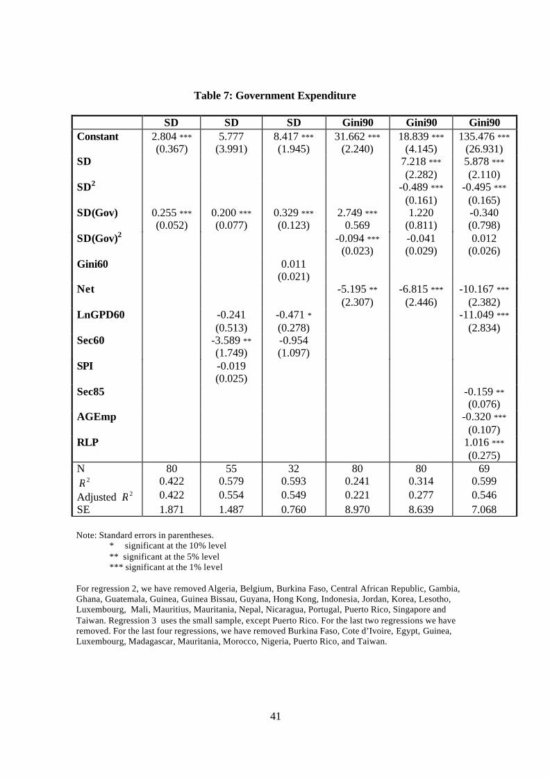
There is a second sense in which our measure of volatility may not be completely
satisfactory. Fluctuations in output growth are likely to be driven by economic or social
variables. In particular, we follow Ramey and Ramey (1995) and investigate the impact
of government spending as a source of volatility. Let Gov be the annual rate of growth of
real government expenditure, and SD(Gov) its standard deviation over the period 1960-
90. We regress the standard deviation of the rate of growth of output on that of the rate of

18
growth of government expenditure. We can see in Table 7, column 1, that this variable is
a major determinant of the volatility of output growth (as found by Ramey and Ramey,
1995). In the next two columns we add other variables to the regression equation. Socio-
political instability is an obvious candidate to try to explain the volatility of output
growth. We also test for the effect of initial inequality (measured by the Gini coefficient
in 1960) on volatility. Neither of these variables has a significant effect.
Table 7 around here
The last three columns of table 7 compare the effect that the volatility of output
growth and of government expenditure have on inequality in 1990. Government
expenditure volatility has a positive and significant impact on inequality, but this effect
disappears once we include the standard deviation of output growth, indicating that
government expenditure affects inequality in so far as it makes output more volatile. We
tried alternative specifications, and obtained similar results when we used as our measure
of volatility the standard deviation of government expenditure as a proportion of GDP.
The average rate of growth of government expenditure proved to have no significant
effect.
4. Causal Considerations
There is a substantial literature that examines the mechanisms that relate fluctuations in
the rate of growth with the mean rate of growth of output.6 However, no work has been
done so far on why fluctuations may affect the distribution of income. This section
proposes a possible explanation for our findings that greater volatility increases
6 Examples of this are Kydland and Prescott (1982), Long and Plosser (1983), and Ramey and Ramey (1991). See Ramey and
Ramey (1995) for a discussion of these models.

19
inequality across countries. We present a simple model of an economy with workers and
managers. If managers are less risk-averse than workers, the degree of riskiness of the
production technology will affect the share of output obtained by each group and hence
the distribution of income.
Consider an economy that consists of workers and managers. There are two
differences between them. First, managers have direct access to the manufacturing
production technology, while workers do not. A worker can either be employed by a
manager in manufacturing, or use a backyard technology by herself. Second, they differ
in their degree of risk-aversion. Workers are assumed to be more risk-averse than
managers, that is, their utility function is more concave. For simplicity of exposition we
will assume that managers are risk-neutral, although this is not necessary for the results.
Let workers' utility be given by U(I), where 0>I represents income. U(I) is a Von
Neumann Morgenstern utility function, such that the first and second derivatives with
respect to income, IU and IIU , exist and are continuous, and 0>IU and 0<IIU .
One can think of this situation as the extreme version of a model in which both
types of agents have the same utility function, which exhibits decreasing absolute risk-
aversion. Richer individuals are thus more willing to accept a certain amount of risk than
poorer individuals. Hence, if managers have accumulated wealth and workers do not, the
former will choose to bear more risk.
When a worker uses the backyard technology, her output at time t is 1−⋅= tt yzz ,
where z is a constant parameter. When an entrepreneur employs a worker, output is
produced according to the risky technology
1−= ttt yy σ , (1)

20
where 1−ty is last period’s output and tσ is the value taken by a non-degenerate random
parameter. The random variable σ is the economy-wide level of technology (it could
also be interpreted as a demand parameter affecting output). Its density function is given
by f(σ ), with support ],0[ Ω∈σ , where ∞<Ω<0 , and mean σ .
A greater dispersion of the distribution of σ implies that managers face greater
risk. It also affects the aggregate rate of growth. Let the number of workers be normalised
to one, so that the rate of growth is given by 1/ 1 −= −ttt yyg (we will show below that,
in equilibrium, the backyard technology is never employed). Using equation (1), we can
express it as 1−= ttg σ . A greater dispersion of the distribution of σ then also implies
that the growth rate is more volatile over time.
The sequence of events is as follows. An entrepreneur hires workers and offers
them contracts that specify their wages. The state of the world, i.e. the value of σ , is then
realized, and all agents observe it. Wages are then paid. Given the timing we have just
described, it is possible to make wages conditional on the realization of the shock.
For simplicity, suppose that managers may offer only two types of contracts: they
could either pay workers a fraction of their random output at each point in time, or they
could pay a constant wage. Suppose that when a random-wage contract is offered,
workers and managers bargain over how to share output. Let β be the (given) share
received by workers and )1( β− that received by the entrepreneur, where )1,0(∈β . We
assume that z>σβ , as otherwise workers would always choose to use the backyard
technology. Under a random wage, the expected utility of a worker is
∫Ω
− ⋅⋅=⋅0 1 )()()( σσββ dFyUyEU tt . (2)

21
If the worker is offered a constant wage w, her expected utility is simply ( )twU ; while if
she is not employed in manufacturing and uses the backyard technology, she obtains
( )tzU .
Managers will prefer to offer a fixed-wage contract if the expected profits it
generates are greater than those from a random-wage contract. That is, if
ttttt yyEwywE σββπσπ ⋅−=⋅>−= −− )1()()()( 11 . (3)
This expression reduces to tt wy >⋅ −1σβ . From the point of view of the entrepreneur, the
optimal constant wage is the lowest wage that would make a worker prefer to work under
a fixed-wage than under a random-wage contract. That is, it is the wage that makes the
worker indifferent between the two types of contract, subject to the constraint imposed by
the outside option (the possibility of working with the backyard technology). The wage
offered by the manager, *tw , is then defined by
( ) ( ) ttt zUyEUwU ,max)( * ⋅= β . (4)
Since workers are risk-averse, the certainty equivalent wage is lower than the expected
random wage. That is, ttt zwy ≥>⋅ −*
1σβ , which implies that equation (3) always holds.
All managers will therefore offer the (bounded) certainty equivalent wage *tw ,
and all workers will be willing to accept it. The expected income shares of the two groups
are given by
1
*
−
=t
tW y
wS
σand .1
1
*
−
−=t
tE y
wS
σ(5)
We now want to examine the effect of an increase in the volatility of output
growth on the income of the two types of individuals. Consider two possible distributions
22
of the random productivity level. Denote the two distributions by R and R′ , and suppose
that R′ is “more risky” on the sense that it is a mean-preserving spread (MPS) of R.
Recall that the wage is determined by ( ) ( )1* )( −⋅= tRt yUERwU σβ , where (.)UER is the
value of a worker’s expected utility when the distribution of σ is given by R. Because
workers’ utility function is concave, a mean preserving spread of the distribution of σ
reduces expected utility. That is, )()( 11 −′− ⋅>⋅ tRtR yUEyUE σβσβ , and hence the certainty
equivalent wage is greater for the less risky distribution, )()( ** RwRw tt ′> . Consequently,
expected profits are greater for R′ than for R, and the share of managers in total output,
as given by equation (5) is also greater for the more risky distribution.
The intuition for this result is simple. Because managers are less risk-averse than
workers, they are willing to bear more risk (under our assumption of risk-neutrality they
bear all the risk). This implies that they can extract a risk premium from workers and
hence increase their profits. The more risky the economy is, the greater the risk premium
–i.e. the lower the wage– and the higher the income received by managers is. More
volatility is hence associated with greater inequality, as it raises the income share of the
top income group.
The impact of volatility on inequality is, however, bounded. As risk keeps
increasing, the certainty equivalent wage falls. It will eventually reach the lower bound
imposed by the backyard technology, tt zRw =′)(* . If the riskyness of σ increases any
more, entrepreneurs cannot further reduce the wage, as this would result in all workers
choosing to leave manufacturing. The wage thus remains at tz . Consequently, for very
high levels of volatility, the relationship between inequality and volatility breaks down.
23
5. Conclusions
Policy-makers are often concerned by macroeconomic volatility, and electoral programs
are often full of references to “attaining economic stability”. This paper has demonstrated
one reason why that concern is well founded: macroeconomic volatility affects the degree
of income inequality in an economy.
Our analysis of cross-country data shows that greater volatility, measured by the
standard deviation of the rate of growth of output, is associated with a higher degree of
inequality. This relationship is robust to controls for all the factors that previous research
has shown to be determinants of income inequality. In fact, volatility, together with
relative labour productivity in agriculture and the share of employment in agriculture,
prove to be the most robust factors affecting income distribution. In order to understand
how volatility affects the distribution of income, we have examined its impact on the
income shares of the various quintiles. Greater volatility results in a redistribution from
middle-income groups (second and third quintiles) to the top-income group (fifth
quintile), while its effect on the share of the lowest 20% of the population is weak.
We have presented a simple model in which greater volatility is associated with a
higher degree of inequality. High income individuals (managers) are characterized by a
lower degree of risk-aversion than workers, and hence insure the latter. In this context,
greater volatility of output, by increasing risk, shifts income from managers to workers
and thus increases the degree of inequality. There are, of course, other possible
mechanisms through which output fluctuations can affect distribution. For example, if
education investments are characterised by fixed costs and capital markets are imperfect,
the level of output will determine whether or not low-income dynasties can invest in

24
education. The degree of volatility may then affect the distribution of human capital, and
hence that of income. There could also be a loss of human capital if, in bad periods, those
with less skills become unemployed and lose skills. Next period, the difference in skills
(and hence wages) between these workers and those who remained in employment would
be even greater.
A detailed examination of these mechanisms is needed if we want to fully
understand the impact of volatility on inequality. However, the relationship that we have
identified has in itself important implications for policy making, as it challenges the long-
standing argument that distributional targets may be incompatible with efficiency goals.
Policies aimed at ensuring macroeconomic stability will at the same time reduce the
degree of income inequality in an economy.
25
References
Aghion, P., Caroli, E. and García-Peñalosa, C. 1998: “Inequality and Economic Growth:
The Perspective from the New Growth Theories”, mimeo, Nuffield College.
Alesina, A. and Perotti, R. 1996: “Income Distribution, Political Instability and
Investment”, European Economic Review 109(2): 465-90.
Alesina, A. and Rodrik, D. 1994: “Distributive Politics and Economic Growth”,
Quarterly Journal of Economics 109: 465-90.
Anand, S and Kanbur, S.M.R. 1993a: “The Kuznets Process and the Inequality-
Development Relationship”, Journal of Development Economics 40(1): 25-52.
Anand, S and Kanbur, S.M.R. 1993b: “Inequality and Development: A Critique”, Journal
of Development Economics 41(1): 19-43.
Atkinson, A.B. 1996: “Seeking to Explain the Distribution of Income”, in New
Inequalities: The Changing Distribution of Income and Wealth in the United
Kingdom. John Hills, ed. Cambridge: Cambridge University Press: 19-48.
Atkinson, A.B. 1997: “Bringing the Income Distribution in from the Cold”, Economic
Journal, 107(441): 297-321.
Barro, R.J. and Lee, J.-W. 1993: “International Comparisons of Educational Attainment”,
Journal of Monetary Economics, 32 (3): 363-94.
Bourguignon, F. and Morrisson, C. 1990. “Income distribution, development and foreign
trade: a cross-section analysis”, European Economic Review, 34 (): 1113-32.
Bourguignon, F. and Morrisson, C. 1998. “Inequality and development and: the role of
dualism”, Journal of Development Economics, 57 (): 233-57.
Chen, S., Datt G. and Ravaillon, M. 1994. “Is Poverty increasing in the Developing
World?”, Review of Income and Wealth, 40 (4): 359-76.
Deininger, K. and Squire, L. 1996: “Measuring income inequality: a new data base”, The
World Bank Economic Review 10 (3): 565-591.
FAO. 1992. Production yearbook, Food and Agriculture Organization, Rome.
Fiszbein, Ariel and George Psacharopoulos. 1995. “Income Inequality Trends in Latin
America”, in Nora Lustig, ed. Coping with Austerity: Poverty and Inequality in
Latin America, The Brookings Institution, Washington.
Gastil, R. Freedom in the World, Westport: Greenwood.

26
Gottschalk, Peter and Timothy M. Smeeding 1997 ‘Cross-National Comparisons of
Earnings and Income Inequality’ Journal of Economic Literature, 35: 633-687.
Hausmann, R., and Gavin, M. 1996: “Securing Stability and Growth in a Shock Prone
Region: The Policy Challenges for Latin America”, in Hausmann, R. and Reisen,
H. (eds.) Securing Stability and Growth in Latin America, OECD Paris.
King, R.G. and Levine, R. 1993: “Finance, Managership, and Growth: Theory and
Evidence”, Journal of Monetary Economics 32 (3): 513-42..
Kuznets, S. 1955: “Economic Growth and Income Inequality”, American Economic
Review 45 (1): 1-28.
Kuznets, Simon. 1963. “Quantitative Aspects of the Economic Growth of Nations”,
Economic Development and Cultural Change, 11(2): 1-80.
Levine, R. and Renelt, D. 1992: “A Sensitivity Analysis of Cross-Country Growth
Models” American Economic Review 82: 942-63.
Li, H., Squire, L. and Zou, H.-F. 1998: “Explaining International and Intertemporal
Variations in Income Inequality”, Economic Journal 108: 26-43.
Kihlstrom, R.E. and Laffont, J.-J. 1979: “A General Equilibrium Entrepreneurial Theory
of Firm Formation Based on Risk Aversion”, Journal of Political Economy 87(4):
719-748.
Kuznets, S. 1955: “Economic Growth and Income Inequality”, American Economic
Review, 45: 1-28.
Kydland, F.E. and Prescott, E.C. 1982: “Time to Build and Aggregate Fluctuations”,
Econometrica, 50(6): 1345-70.
Long, J.B. and Plosser, C.I. 1983: “Real Business Cycles”, Journal of Political Economy,
91(1): 39-69.
Perotti, R. 1996: “Growth, Income Distribution and Democracy: What the Data Say”,
Journal of Economic Growth, 1: 149-187.
Pritchett, L. 1998. “Patterns of Economic Growth: Hills, Plateaus, Mountains, and
Plains”, miemo, World Bank.
Ramey, G. and Ramey, V.A. 1995: “Cross-Country Evidence on the Link Between
Volatility and Growth”, American Economic Review, 85(5): 1138-1151.

27
Ramey, G. and Ramey, V.A. 1991: “Technology Commitment and the Cost of Economic
Fluctuations”, NBER Working Paper: 3755.
Summers, and Heston : “Penn World Tables, Mark 5.6”.
World Bank. 1993. World Tables.World Bank. 1996: World Development Report.

28
Appendix: Data Sources and Main Data
A.1. Inequality
Almost all the data on inequality is from Deininger and Squire (1996), obtained from the
World Bank Webb Site (version 13/6/97). We first selected all the observations that were
obtained from surveys of national coverage, for the years of interest (or as close as
possible, ranging between 1984 and 1995). This implied that for many countries there
were several observations for the same year, in some cases giving rather different values.
For the OECD we chose the observations recommended by Atkinson and Brandolini
(1999). This means that we have, in most cases, used the LIS data. For Italy in 1991 we
have used the data available in the LIS Webb site, following the suggestion of Atkinson
and Brandolini. For developing countries, we have mainly used the data from Chen, Datt
and Ravaillon (1994) and the World Development Report, as reported by Deininger and
Squire. When, exceptionally, the data from these two sources differed, we have computed
an average value (this was the case for Tanzania, Zambia and Venezuela). Whenever
possible, we have used observations of the distribution of income rather than expenditure.
For this reason, the observation we have used for Bangladesh is that for 1986, rather than
those for 1989 and 1990. We also selected observations that reported the distribution of
gross (rather than net) and personal or person equivalent (rather than household) income.
This was not always possible.
GINIxx: Gini coefficient of income in or around the year 19xx.
Qy,xx: Income share of the yth quintile in or around the year 19xx.
Net: Dummy variable taking the value 1 if the inequality measure is based on net income,
and 0 if it is based on gross income.
29
A.2. Output and volatility
LnGDPXX: Logarithm of real per capita GDP in the year 19XX. The output variable
used is real GDP per capita in 1985 constant dollars (Chain Index).
SD: Standard deviation of the rate of output growth. Output is real per capita GDP. We
calculate the annual rate of growth of over the period 1960 to 1990, and then the standard
deviation of annual growth rates.
Growth60-90: Average annual rate of growth of real per capita GDP over 1960 to 1990.
SD(∆g): Standard deviation of the year to year changes in the annual rate of output
growth, over the period 1960 to 1990.
Gov: Annual rate of growth of real government expenditure (1985 prices). Obtained by
multiplying the real government share of GDP by real per capita GDP.
SD(Gov): Standard deviation of the annual rate of growth of real government expenditure
over the period 1960-90.
Source: Summers and Heston, Penn World Tables Mark 5.6.
A.3. Education
Sec85: Percentage of “secondary schooling attained” in the total population in 1985.
MYSch: mean years of secondary schooling in the total population in 1960.
Source: Barro and Lee (1993).
A.4. Agriculture
AgEmp: Percentage of the economically active population employed in agriculture.
Land pc: Arable land and land under permanent crops in 1991 (in 1000 Ha) divided by
the total population in 1990 (in 1000s).
Source: FAO Production yearbook, 1992, Tables 1 and 3.
30
AgShare: Agricultural output as a share of GDP. Three years averages (for 1988, 1989,
and 1990) are used in order to smooth possible fluctuations in agricultural prices. For
some countries the data are for 1987-89, for Peru it is for 1978-80.
Source: World Bank World Tables 1993.
RLP: Relative labour productivity (non-agriculture/agriculture). Calculated as RLP=(1-
AgShare)AgEmp/((1-AgEmp)AgShare).
A.5. Other variables
CIVLIB: Index of civil liberties, averaged over 1960-89. A value of 1 is assigned to
countries with the largest degree of civil liberties, and 7 to those with the smallest.
FNDV (M1Y): Degree of financial development, measured by the ratio of M1 to GDP
averaged over 1960-1989.
FNDV (LLY): Degree of financial development, measured by the ratio of liquid
liabilities to GDP averaged over 1960-1989.
INV: Investment share in GDP, averaged over the period 1960-89.
TRD: Ratio of total trade (imports plus exports) to GDP, averaged over 1960-89.
X: export share of GDP, averaged over the period 1960-89.
TRDG: Growth of the ratio of total trade to GDP between 1960 and 1990.
Source of all the above: King and Levine (1993). The names of the variables in the
original data set are, respectively, CIVL, LLY, INV, TRD, X, TRDG.
SPI: Index of socio-political instability over the period 1960-85, where a higher value
indicates more instability. From Alesina and Perotti (1996)
31
Table A.1: Main Data for the 80-Country Sample
Country Gini SD Country Gini SDAlgeria 38.73 7.553 Korea, R. 33.64 4.097Australia 35.93 2.698 Lesotho 60.90 7.443Austria 31.60 1.74 Luxembourg 23.81 4.203Bangladesh 37.00 8.961 Madagascar 43.44 4.229Belgium 29.24 2.218 Malawi 62.00 5.043Bolivia 42.04 3.473 Malaysia 48.35 4.926Botswana 54.21 8.582 Mali 54.00 5.371Brazil 63.42 4.624 Mauritania 42.53 6.820Burkina Faso 39.00 4.703 Mauritius 36.69 8.308C. Afr. Rep. 55.00 4.171 Mexico 54.98 4.220Canada 32.73 2.486 Morocco 39.20 5.514Chile 56.49 6.458 Nepal 30.06 7.460Colombia 51.32 2.448 Netherlands 29.10 2.139Costa Rica 46.07 3.739 New Zealand 36.58 2.957Cote d'Ivoire 38.00 6.562 Nicaragua 50.32 9.268Denmark 28.75 2.726 Niger 36.10 9.841Dom. Rep. 50.46 6.843 Nigeria 41.15 11.160Ecuador 43.00 4.774 Norway 27.29 1.900Egypt 32.00 3.362 Pakistan 32.38 4.231Finland 26.31 3.000 Panama 56.47 5.726France 33.52 1.879 Peru 44.87 6.598Gambia 39.00 9.760 Philippines 45.73 3.585Germany 26.00 2.250 Portugal 36.76 4.364Ghana 36.74 7.069 Puerto Rico 50.86 3.672Greece 37.67 3.732 Senegal 54.12 4.274Guatemala 59.06 3.071 Singapore 41.00 4.802Guinea 40.40 6.411 South Africa 62.30 3.689Guin. Bissau 56.12 9.455 Spain 25.91 3.253Guyana 40.22 11.773 Sri Lanka 46.70 4.643Honduras 52.63 2.978 Sweden 26.31 1.760Hong Kong 45.00 4.020 Taiwan 30.53 2.805India 32.53 5.029 Tanzania 48.56 6.046Indonesia 33.09 3.960 Thailand 50.80 3.408Iran 42.90 9.468 Tunisia 40.24 3.362Ireland 37.90 2.580 Turkey 44.09 3.536Italy 29.00 2.667 UK 34.32 2.198Jamaica 41.79 4.917 USA 38.51 2.439Japan 35.00 3.526 Venezuela 48.96 4.276Jordan 40.66 10.118 Zambia 47.46 6.509Kenya 54.39 7.681 Zimbabwe 56.83 5.731
Average 41.98 4.99
32
Table A.2: Main Data for the 33-Country Sample
Country Gini90 Gini60 Q5,90 Q5,60 SD NetAustralia 35.93 32.00 0.42 0.39 2.70 0Brazil 63.42 54.00 0.67 0.62 4.62 0Canada 32.73 30.80 0.39 0.35 2.49 0Colombia 51.32 62.00 0.54 0.68 2.45 0Costa Rica 46.07 50.00 0.51 0.60 3.74 0Denmark 28.75 37.00 0.36 0.41 2.73 0Finland 26.31 46.00 0.35 0.49 3.00 0France 33.52 50.00 0.41 0.54 1.88 0Hong Kong 45.00 46.20 0.49 0.57 4.02 0India 32.53 32.59 0.42 0.41 5.03 1Indonesia 33.09 33.30 0.42 n.a. 3.96 1Japan 35.00 37.20 n.a. 0.44 3.53 0Korea, R. 33.64 34.34 0.42 0.42 4.10 0Malaysia 48.35 36.00 0.54 0.44 4.93 0Mexico 54.98 53.00 0.59 0.60 4.22 0Netherlands 29.10 42.00 0.37 0.48 2.14 0New Zealand 36.58 35.70 0.42 n.a. 2.96 0Norway 27.29 35.00 0.36 0.41 1.90 0Pakistan 32.38 34.70 0.35 n.a. 4.23 0Panama 56.47 50.02 0.60 n.a. 5.73 0Philippines 45.73 48.00 0.53 0.56 3.58 0Puerto Rico 50.86 52.32 0.53 0.54 3.67 0South Africa 62.30 55.00 0.65 n.a. 3.69 0Sri Lanka 46.70 47.00 0.52 0.52 4.64 0Sweden 26.31 35.74 0.35 0.40 1.76 0Taiwan 30.53 32.24 0.39 0.41 2.81 0Tanzania 48.56 39.00 0.54 n.a. 6.05 1Thailand 50.80 41.28 n.a. 0.50 3.41 0Tunisia 40.24 42.30 0.46 0.49 3.36 1Turkey 44.09 56.00 0.50 0.60 3.54 0UK 34.32 29.68 0.41 0.38 2.20 0USA 38.51 35.69 0.43 0.41 2.44 0Venezuela 48.96 42.00 0.54 0.48 4.28 0Average 40.92 42.06 0.47 0.49 3.51

33
Figure 1:Volatility and the Gini Coefficient
0
10
20
30
40
50
60
70
0 2 4 6 8 10 12 14Standard Deviation 1960-90
Gin
i Co
effi
cien
t 19
90

34
Figure 2:Volatility and the Gini Coefficient by Region
OECD
NICsAsia
Africa
Latin America
0
10
20
30
40
50
60
0 1 2 3 4 5 6 7
Standard Deviation 1960-90
Gin
i Co
effi
cien
t

35
Table 1: Gini Coefficient Analysis
Gini90 Gini90 Gini90 Gini90 Gini90 Gini90Constant 16.033 ***
(3.694)-43.258(54.782)
13.927(57.068)
66.888 ***(13.197)
34.775 ***(5.136)
32.094 ***(6.568)
SD 10.067 ***(1.470)
5.171 ***(1.593)
5.833 ***(1.553)
8.020 ***(1.477)
7.846 ***(1.621)
SD2 -0.680 ***
(0.112)-0.407 ***
(0.116)-0.453 ***
(0.117)-0.611 ***
(0.122)-0.577 ***
(0.114)Net -6.320 ***
(2.367)-7.917 ***
(2.106)-8.213 ***
(2.585)-8.757 ***
(2.602)-8.586 ***
(2.513)-7.853 ***
(2.634)LnGPD90 29.322 **
(13.538)10.188
(14.655)-3.845 ***
(1.343)(LnGPD90)2 -2.220 ***
(0.827)-0.892(0.919)
Sec85 -0.162 **(0.075)
-0.187 ***(0.074)
-0.282 ***(0.071)
-0.323 ***(0.080)
Growth60-90 -1.438 ***
(0.536)Investment 1.058
(22.16)N 80 80 70 70 70 68
2R 0.291 0.413 0.505 0.498 0.495 0.463Adjusted 2R 0. 273 0.398 0.466 0.467 0.464 0.429Standard Error 8.671 7.886 7.677 7.665 7.686 7.892
Note: Standard errors in parentheses.* significant at the 10% level** significant at the 5% level*** significant at the 1% level
Due to data availability, we have removed Burkina Faso, Cote d’Ivoire, Egypt, Guinea, Luxembourg,Madagascar, Mauritania, Morocco, Nigeria, and Puerto Rico from the last four regression equations. Forthe last one, we have also removed Nepal and Taiwan.
36
Table 2: Regional Dummies and Dualism
Gini90 Gini90 Gini90 Gini90Constant 25.247 ***
(3.384)-0.947
(75.742)117.752 *(69.541)
56.460(104.4)
SD 4.271 ***(1.621)
3.788 **(1.650)
5.252 ***(1.467)
7.728 ***(2.399)
SD2 -0.316 ***
(0.109)-0.312 ***
(0.121)-0.450 ***
(0.115)-0.665 ***
(0.221)Net -8.181 ***
(1.899)-8.859 ***
(2.143)-10.040 ***
(2.443)-8.733 ***
(3.063)LnGDP90 10.264
(19.037)-7.117
(15.884)4.123
(23.939)(LnGPD90) 2 -0.726
(1.177)-0.220(0.932)
-0.802(1.402)
Sec85 -0.116 *(0.069)
-0.159 ** (0.075)
-0.093 (0.076)
LatinAmerica
15.863 ***
(2.323)10.997 ***
(3.472)Africa 15.747 ***
(3.274)13.482 ***
(5.064)Asia 7.529 **
(3.683)2.663
(4.825)NIC 2.392
(3.403)0.975
(3.654)Land pc 1.607 *
(0.887)AgEmp -0.309 ***
(0.111)-0.268 **
(0.135)RLP 0.972 ***
(0.302)0.987 ***
(0.319)SPI -0.0503
(0.101)N 80 70 69 50
2R 0.559 0.629 0.601 0.665
Adjusted 2R 0.523 0.573 0.548 0.600Standard Error 7.027 6.861 7.049 6.827
Note: Standard errors in parentheses.* significant at the 10% level** significant at the 5% level*** significant at the 1% level
For all but the first regression, we have removed Burkina Faso, Cote d’Ivoire, Egypt, Guinea, Luxembourg,Madagascar, Mauritania, Morocco, Nigeria, and Puerto Rico, due to data availability. For regression 3 wehave also removed Taiwan. For the last regression we have also removed Algeria, Belgium, CentralAfrican Republic, Gambia, Ghana, Guatemala, Guinea Bissau, Guyana, Hong Kong, Indonesia, Jordan,Korea, Lesotho, Mali, Mauritius, Nepal, Nicaragua, Portugal, Singapore and Taiwan.

37
Table 3: Financial Development and Civil Liberties
Gini90 Gini90 Gini90 Gini90 Gini90 Gini90Constant 37.925 ***
(3.820)37.945 ***
(4.451)38.190 ***
(5.732)35.164 ***
(6.059)92.904
(70.658)91.604
(71.567)
SD 4.177 **(1.702)
4.921 ***(1.758)
3.681 **(1.703)
4.106 **(1.699)
SD2 -0.336 ***(0.126)
-0.388 ***0.135
-0.345 ***(0.126)
-0.379 ***(0.124)
Net -7.023 **
(2.758)-7.874 ***
(2.622)-8.617 ***
(2.864)-9.334 ***
(2.573)MYSch 0.618
(1.558)1.025
(1.759)LnGDP90 -1.6577
(16.735)-1.146
(16.836)(LnGPD90) 2 0.461
(1.007)-0.553(1.013)
Sec85 -0.243 ***(0.080)
-0.214 ***(0.080)
-0.156 **(0.078)
-0.118(0.076)
CIVLIB 2.830 ***
(0.734)2.463 ***
(0.749)1.584 *(0.841)
1.523 *(0.875)
0.844(0.746)
0.719(0.730)
FNDV (M1Y) -34.118***
(9.508)-19.139 *(9.833)
-13.804(12.793)
FNDV (LLY) -13.625 **(5.578)
-6.567(4.366)
-1.037(5.556)
AgEmp -0.306 ***(0.108)
-0.307 *** (0.108)
RLP 0.991 **(0.504)
1.007 **(0.498)
N 62 63 61 62 61 622R 0.352 0.344 0.521 0.520 0.615 0.622
Adjusted 2R 0.330 0.322 0.477 0.477 0.564 0.573Standard Error 8.142 8.309 7.197 7.302 6.709 6.733
Note: Standard errors in parentheses.* significant at the 10% level** significant at the 5% level*** significant at the 1% level
For all regressions, we have removed Botswana, Burkina Faso, Cote d’Ivoire, Guinea, Guyana, HongKong, Lesotho, Luxembourg, Madagascar, Mauritania, Morocco, Nepal, Nigeria, Puerto Rico, Taiwan, andZimbabwe, due to data availability. For regression 1 we have also removed Chile and Sweden; forregression 2, Mexico; for regressions 3 and 5, Chile, Egypt and Sweden; for regressions 4 and 6, Egypt andMexico.

38
Table 4: Quintile Analysis
Q5,90 Q4,90 Q3,90 Q2,90 Q1,90Constant 124. 923 *** 5.637 -6.563 -12.802 -11.188 *
(26.056) (6.707) (7.249) (8.659) (6.622)SD 4.189 *** -0.773 ** -1.539 *** -1.592 *** -0.905 **
(1.223) (0.324) (0.334) (0.397) (0.357)SD2 -0.388 *** 0.057 ** 0.124 *** 0.131 *** 0.076 **
(0.100) (0.026) (0.027) (0.033) (0.030)Net -9.318 *** 2.240 *** 2.525 *** 2.342 *** 2.211 ***
(2.237) (0.880) (0.616) (0.740) (0.557)LnGPD90 -9.262 *** 1.898 *** 2.588 *** 2.822 *** 1.954
(2.745) (0.719) (0.774) (0.915) (0.705)Sec85 -0.124 * 0.027 0.042 ** 0.030 0.024
(0.068) (0.019) (0.020) (0.022) (0.018)AgEmp -0.286 *** 0.043 ** 0.082 *** 0.093 *** 0.067 **
(0.096) (0.019) (0.026) (0.032) (0.028)RLP 0.920 *** -0.187 *** -0.267 *** -0.275 *** -0.189 ***
(0.230) (0.062) (0.067) (0.073) (0.064)N
2RAdjusted 2RSt. Error
590.5860.5386.164
590.4980.4401.772
590.6260.5831.700
590.5150.4592.022
590.4180.3511.645
Note: Standard errors in parentheses.* significant at the 10% level** significant at the 5% level*** significant at the 1% level
For all these regressions, we have removed Burkina Faso, Central African Rep., Cote d’Ivoire, Egypt,Gambia, Germany, Guinea, Iran, Japan, Lesotho, Luxembourg, Madagascar, Malawi, Mali, Mauritania,Morocco, Nigeria, Puerto Rico, Taiwan, Thailand, and Zambia, due to data availability.
39
Table 5: Gini Coefficient Analysis
Gini90 Gini90 Gini90 Gini90 Gini90 Gini90 Gini90Constant 17.556 *** -5.011 -238.966 -50.210 79.109 7.641 -2.216
(3.864) (5.411) (157.86) (121.86) (180.14) (8.867) (12.776)Gini60 0.668 *** 0.495 ** 0.550 ** 0.648 *** 0.604 ***
(0.129) (0.210) (0.244) (0.172) (0.214)SD 7.067 *** 5.270 *** 4.819 *** 4.315 *** 4.565 ***
(1.178) (0.880) (1.260) (1.607) (1.183)Net*SD -2.559 *** -1.152 ** -1.868 -0.975 -1.374
(0.830) (0.544) (1.244) (1.513) (0.946)LnGDP90 72.947 * 8.148 -9.031
(37.113) (26.671) (37.045)(LnGDP90)2 -4.641 ** -0.284 0.037
(2.164) (1.517) (2.009)Latin 9.405 ***
America (3.500)Africa 17.122 ***
(6.518)Asia 10.068*
(5.075)NIC 1.792
(2.622)Sec85 0.025 -0.065 -0.025
(0.093) (0.078) (0.100)Land pc 3.700 ***
(1.383)AgEmp -0.385 *
(0.208)RLP 2.629 *
(1.519)CIVLIB 1.961 ** 0.718
(0.927) (1.190)FNDP (LLY) 5.085 2.622
(6.161) (5.680) N
2R Adjusted 2R St. Error
330.4410.4238.087
330.7060.6865.970
330.3510.3308.715
330.7750.7005.866
310.7730.6905.973
290.5470.4937.629
290.6770.6076.722
Note: Standard errors in parentheses.* significant at the 10% level** significant at the 5% level*** significant at the 1% level
We have used the sample reported in Table A.2. For the last three regressions, we have removed Taiwanand Puerto Rico, due to data availability. For the last two, we have also removed Hong Kong and Mexico.

40
Table 6: Quintile Analysis
Q5,90 Q4,90 Q3,90 Q2,90 Q1,90Constant 113.357 * 5.575 -7.875 -20.134 -22.370 **
(57.570) (5.706) (10.497) (14.317) (10.338)Q5,60 0.212
(0.197)Q4,60 0.060
(0.158)Q3,60 0.372 *
(0.191)Q2,60 0.009
(0.208)Q1,60 -0.164
(0.187)SD 3.731 ** -0.469 -1.231 ** -1.028 * -0.491
(1.575) (0.389) (0.473) (0.510) (0.425)Net*SD -2.563 *** 0.462 *** 0.477 * 0.973 *** 1.055 ***
(0.896) (0.112) (0.243) (0.291) (0.232)LnGDP90 -9.440 * 1.810 ** 2.301 * 3.563 ** 3.176 **
(5.257) (0.800) (1.238) (1.636) (1.084)Sec85 -0.047 0.015 -0.001 0.027 0.025
(0.065) (0.017) (0.021) (0.023) (0.016)AgEmp -0.364 * -0.054 0.091 * 0.135 ** 0.131 ***
(0.189) (0.034) (0.048) (0.058) (0.036)RLP 1.490 -0.600 -0.227 0.537 -0.512
(1.875) (0.366) (0.550) (0.553) (0.364) N
2R Adjusted 2R St. Error
230.8230.7574.390
230.7870.7071.054
230.8500.7941.224
230.7630.6741.520
230.7060.5961.281
Note: Standard errors in parentheses.* significant at the 10% level** significant at the 5% level*** significant at the 1% level
Due to data availability, we have removed Indonesia, Japan, New Zealand, Pakistan, Panama, South Africa,Taiwan, Tanzania, Thailand, and Puerto Rico from all regressions.
41
Table 7: Government Expenditure
SD SD SD Gini90 Gini90 Gini90Constant 2.804 ***
(0.367)5.777
(3.991)8.417 ***(1.945)
31.662 ***(2.240)
18.839 ***(4.145)
135.476 ***(26.931)
SD 7.218 ***
(2.282)5.878 ***
(2.110)SD2 -0.489 ***
(0.161)-0.495 ***
(0.165)SD(Gov) 0.255 ***
(0.052)0.200 ***(0.077)
0.329 ***(0.123)
2.749 ***0.569
1.220(0.811)
-0.340(0.798)
SD(Gov)2 -0.094 ***(0.023)
-0.041(0.029)
0.012(0.026)
Gini60 0.011(0.021)
Net -5.195 **
(2.307)-6.815 ***
(2.446)-10.167 ***
(2.382)LnGPD60 -0.241
(0.513)-0.471 *(0.278)
-11.049 ***
(2.834)Sec60 -3.589 **
(1.749)-0.954(1.097)
SPI -0.019(0.025)
Sec85 -0.159 **(0.076)
AGEmp -0.320 ***
(0.107)RLP 1.016 ***
(0.275)N 80 55 32 80 80 69
2R 0.422 0.579 0.593 0.241 0.314 0.599Adjusted 2R 0.422 0.554 0.549 0.221 0.277 0.546SE 1.871 1.487 0.760 8.970 8.639 7.068
Note: Standard errors in parentheses.* significant at the 10% level** significant at the 5% level*** significant at the 1% level
For regression 2, we have removed Algeria, Belgium, Burkina Faso, Central African Republic, Gambia,Ghana, Guatemala, Guinea, Guinea Bissau, Guyana, Hong Kong, Indonesia, Jordan, Korea, Lesotho,Luxembourg, Mali, Mauritius, Mauritania, Nepal, Nicaragua, Portugal, Puerto Rico, Singapore andTaiwan. Regression 3 uses the small sample, except Puerto Rico. For the last two regressions we haveremoved. For the last four regressions, we have removed Burkina Faso, Cote d’Ivoire, Egypt, Guinea,Luxembourg, Madagascar, Mauritania, Morocco, Nigeria, Puerto Rico, and Taiwan.