03/03/2020

1

* 7.4 text Drivers of Income Distribution Changes https://www.cps.fgv.br/cps/bd/curso/Drivers_IncomeDistribution_Neri_Brazill_Updated_GMD.pdf

*8b Horizontal Inequality, Labor Markets and Education

Marcelo Neri (FGV Social )

***Returns to education and intergenerational mobilityhttps://www.wider.unu.edu/publication/returns-education-intergenerational-mobility-and-inequality-trends-brazil-0

Labor decompositions, Mincerian and Markovian equations, D in D

Measurement Error, Selectivity and Ommited Variable Biases

EDUEDUCATION

JORNADAWORKING TIME

OCUP

PEA

OCCUPIED

PEAPEA

POP

PEA

PIA

N ível

Educa ção

Years of

Schooling JornadaWeekly HoursOcupa ção Occupation Rate Participa ç

ão

Participation Rate

RENDA TOTAL/

REDA TRABALHO

TOTAL INCOME

LABOR EARNINGS

Importância

de outras

Fontes de

Renda

Alternativas a

do Trabalho

Importance

of Alternative

Income Sources

SAL Á RIO

JORNADA

EDUCA Ç ÃO

HOURLY WAGE

EDUCATION

Retorno

da

Educa ç ão

Education

X X X XXRENDA TOTAL

DO JOVEM

TOTAL INCOME =

Premium

other than Labor

Demographic

Bonus

PIA

POP

INCOME POLICIES PRODUCTIVITY WORK EFFORT

Labor Market, Income Policies and Demographic Bonus Decomposition

Labor EconomicsOccupied population (E): People working

Unemployed population (U): People looking

for job but not occupied

Inactive population (I): People not occupied

Active Age Population AAP (PIA):

occupied + unemployed + inactive = (E + U + I)

Economically Active Population EAP (PEA)

occupied + unemployed (E + U )

Participation Rate: (PEA) / (PIA) = ( E + U ) / ( E + U + I )

Unemployment Rate: (Unemployed) / (PEA) = ( U ) / ( E + U )

Occupation Rate in PEA: (Occupied) / (PEA) = ( E ) / ( E + U )

Definitions and Formulas

03/03/2020

2

Mean Earnings =

Hourly-wage by education

Education Working time

Occupied in EAP

EAP in AAP

Unemployment Effect

Participation Effect

Variation Rate (%)2014 / 2019

Total Population

-1,13

-6,28

8,97

-1,92

-4,59

3,45

Source: FGV Social from PNADC/IBGE microdata individual normal Labor Earnings

Individual Earnings Mean Decomposition

Decomposition of Individual Earnings Growth Rates by Classic Labor

Ingredients - per Capita Income Groups from 2014.T4 to 2019.T2

Source: FGV Social/CPS from quarterly PNADC microdata/IBGE- 15 to 59 years of age

-19

% -15

%

11%

-5%

-13%

3,5

%

-4%

-11

%

8%

-1,2

%

-2,7

%

3,1

%

3%

-4%

4%

1%

-0,6

%

3,0%

15%

1,4%

5% 6

%

-0,1

%

1,6%

Renda Total = RetornoEducação X

Educação X Jornada X Desemprego X Participação

50 - 40 + - 10 + 1 +

Total Income = Education Returns XEducation X Journey X Unemployment X Participation

03/03/2020

3

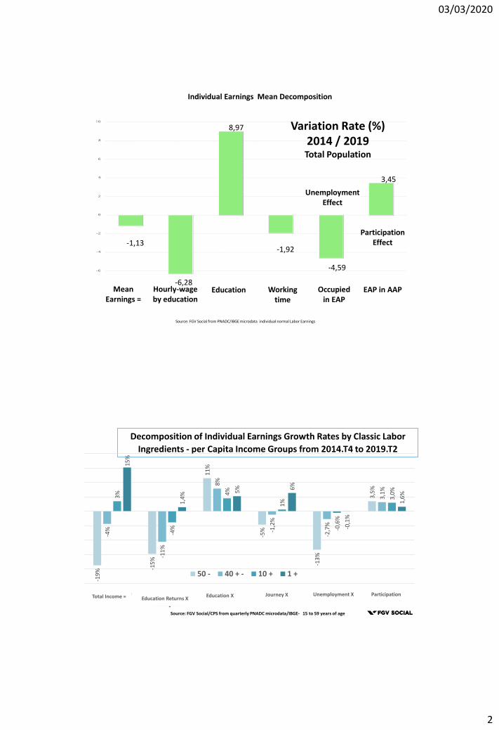
Individual All Sources Incomes Annual Growth Rates - 2001 to 2014

3,6%

4,8%

5,9%

4,9%5,1%

5,6%

6,4%

5,5%

6,0%

3,0%

3,5%

4,0%

4,5%

5,0%

5,5%

6,0%

6,5%

7,0%

Total Northeast Rural Females Blacks Mulattos IlliteratesHeads

Sons Spouses

Source FGV Social from PNAD e PNADC/IBGE microdata

Horizontal Inequality – Individual Income Growth Rate Excluded Groups

-0,49

-3,49

-2,64

-1,35

-2,52

-3,14

-6,50

-3,60

-2,66

-3,01

-1,16

-0,61

-6,33

-8,75

-2,31

-1,50

Total

0 year of study

1 to 3 years of studies

Males

Heads

Sons

Youth 15 to 19

Youth 20 to 24

Youth 25 to 29

More than 6 people

Black

Brown

Aracaju Capital

Recife Periphery

North

Northest

Individual Income from Labor - 15 to 59 years (%.)

Annual Variation from 2014 to 2019

Mincerian Model: (Mincer 1974; Lemieux 2006, Card 2001)

𝑦𝑖 = ln 𝑌𝑖 = 𝛼 + 𝛽𝑆𝑖 + 𝑥𝑖′𝛾 + 𝜀𝑖

where 𝑌𝑖 is the labour income of individual 𝑖 (we change this metric below) , 𝑆𝑖 is the level of education of individual 𝑖 measured by years of schooling, 𝑥𝑖 is a vector of controls and 𝜀𝑖 is an error term.

The Coefficient and Attribute Premium

This is a regression model in the log-level format, that is, the dependent variable, the wage is in logarithmic format and the most

relevant independent variable, schooling, is in level format. Therefore, the coefficient β1 measures how much one year more of

schooling causes in proportional variation in the wage of the individual. For example, if β1 is estimated at 0.18, this means that

each additional year of study is related on average with a wage increase of 18%. This corresponds to the premium of the

attribute (or rate of return if the costs were zero). Mathematically, we have:

Deriving, we find that: ( ∂ ln y / ∂ educ )= β1

On the other hand, by the chain rule, we have:

( ∂ ln y / ∂ educ ) = ( ∂ y / ∂ educ ) ( 1 / w ) = ( ∂ y / ∂ educ ) / y)

Thus, β1=(∂ y /∂educ)/ y, corresponds to the percentage variation of the wage from a increase of one year of study..

The coefficient of the mincerian regression with only the constant and a specific variable, say education, gives the gross or

uncontrolled relative premium in terms of income variation.

The coefficient of a variable of a multivariate mincerian regression (that is, a log-linear equation with a constant and a series of

additional variables) gives us the marginal controlled relative premium in terms of income variation. Thus, a tentative to isolate

the effect of this variable from the possible correlations with the other variables considered.

03/03/2020

4

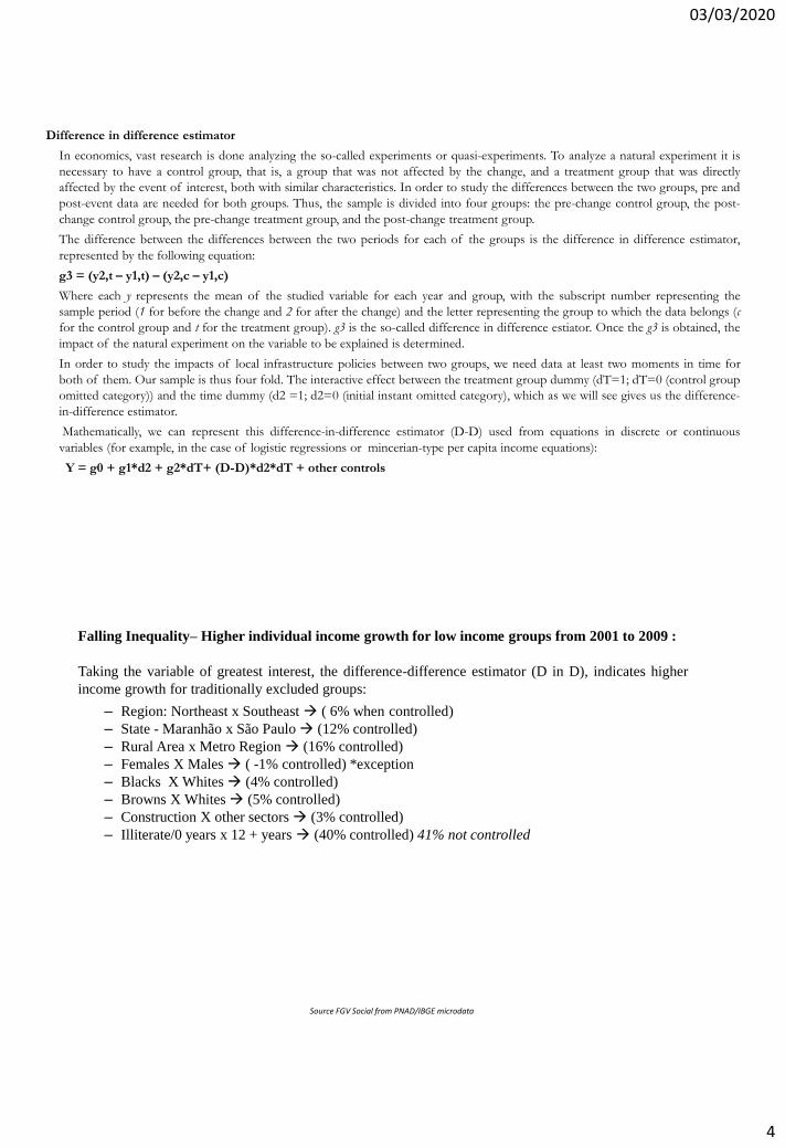
Difference in difference estimator

In economics, vast research is done analyzing the so-called experiments or quasi-experiments. To analyze a natural experiment it is

necessary to have a control group, that is, a group that was not affected by the change, and a treatment group that was directly

affected by the event of interest, both with similar characteristics. In order to study the differences between the two groups, pre and

post-event data are needed for both groups. Thus, the sample is divided into four groups: the pre-change control group, the post-

change control group, the pre-change treatment group, and the post-change treatment group.

The difference between the differences between the two periods for each of the groups is the difference in difference estimator,

represented by the following equation:

g3 = (y2,t – y1,t) – (y2,c – y1,c)

Where each y represents the mean of the studied variable for each year and group, with the subscript number representing the

sample period (1 for before the change and 2 for after the change) and the letter representing the group to which the data belongs (c

for the control group and t for the treatment group). g3 is the so-called difference in difference estiator. Once the g3 is obtained, the

impact of the natural experiment on the variable to be explained is determined.

In order to study the impacts of local infrastructure policies between two groups, we need data at least two moments in time for

both of them. Our sample is thus four fold. The interactive effect between the treatment group dummy (dT=1; dT=0 (control group

omitted category)) and the time dummy (d2 =1; d2=0 (initial instant omitted category), which as we will see gives us the difference-

in-difference estimator.

Mathematically, we can represent this difference-in-difference estimator (D-D) used from equations in discrete or continuous

variables (for example, in the case of logistic regressions or mincerian-type per capita income equations):

Y = g0 + g1*d2 + g2*dT+ (D-D)*d2*dT + other controls

Falling Inequality– Higher individual income growth for low income groups from 2001 to 2009 :

Taking the variable of greatest interest, the difference-difference estimator (D in D), indicates higher

income growth for traditionally excluded groups:

– Region: Northeast x Southeast ( 6% when controlled)

– State - Maranhão x São Paulo (12% controlled)

– Rural Area x Metro Region (16% controlled)

– Females X Males ( -1% controlled) *exception

– Blacks X Whites (4% controlled)

– Browns X Whites (5% controlled)

– Construction X other sectors (3% controlled)

– Illiterate/0 years x 12 + years (40% controlled) 41% not controlled

Source FGV Social from PNAD/IBGE microdata

03/03/2020

5

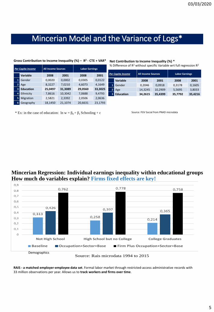
Per Capita Income All Income Sources Labor Earnings

Variable 2008 2001 2008 2001

1 Gender 0,0020 0,0002 0,0305 0,0122

2 Age 8,3227 7,0210 4,6073 4,1649

3 Education 25,0497 31,3089 29,0560 33,3025

4 Ethnicity 7,8616 10,3042 7,0688 9,4793

5 Migration 2,5821 2,3392 2,0506 2,0636

6 Geography 18,1450 21,1074 20,6631 23,1793

Gross Contribution to Income Inequality (%) – R2 - CTE + VAR*

* Ex: in the case of education: ln w = β0 + β1 Schooling + є

Net Contribution to Income Inequality (%) *% Difference of R2 without specific Variable wrt full regression R2

Per Capita Income All Income Sources Labor Earnings

Variable 2008 2001 2008 2001

1 Gender 0,2046 0,0918 0,3178 0,1605

2 Age 14,3245 10,2909 5,5695 3,8033

3 Education 34,2615 35,4399 35,7792 35,4216

Source: FGV Social from PNAD microdata

Mincerian Model and the Variance of Logs*

Mincerian Regression: Individual earnings inequality within educational groups How much do variables explain? Firms fixed effects are key!

Source: Rais microdata 1994 to 2015 Demographics

RAIS - a matched employer-employee data set. Formal labor market through restricted-access administrative records with 33 million observations per year. Allows us to track workers and firms over time.

03/03/2020

6

Returns to education and intergenerational mobilityMotivation:

• Address Measurement error: make use of the information of who responded to the PNAD questionnaire on income and education, as a proxy for measurement error.

Research Questions:

03/03/2020

7

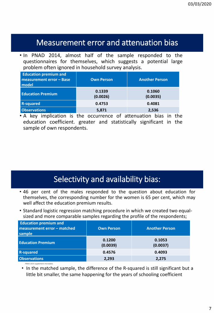
Measurement error and attenuation bias

• In PNAD 2014, almost half of the sample responded to thequestionnaires for themselves, which suggests a potential largeproblem often ignored in household survey analysis.

• A key implication is the occurrence of attenuation bias in theeducation coefficient. greater and statistically significant in thesample of own respondents.

Education premium and measurement error – Base model

Own Person Another Person

Education Premium0.1339

(0.0026)0.1060

(0.0035)

R-squared 0.4753 0.4081

Observations 5,871 2,536PNAD 2014 supplement microdata.

Selectivity and availability bias:

• 46 per cent of the males responded to the question about education forthemselves, the corresponding number for the women is 65 per cent, which maywell affect the education premium results.

• Standard logistic regression matching procedure in which we created two equal-sized and more comparable samples regarding the profile of the respondents;

Education premium and measurement error – matched sample

Own Person Another Person

Education Premium0.1200

(0.0039)0.1053

(0.0037)

R-squared 0.4576 0.4093

Observations 2,293 2,275

• In the matched sample, the difference of the R-squared is still significant but alittle bit smaller, the same happening for the years of schooling coefficient

PNAD 2014 supplement microdata.

03/03/2020

8

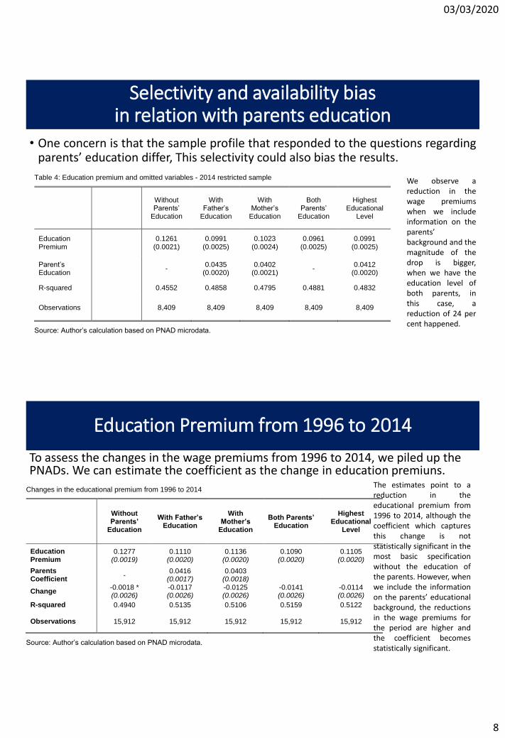
Selectivity and availability bias in relation with parents education

• One concern is that the sample profile that responded to the questions regardingparents’ education differ, This selectivity could also bias the results.

Table 4: Education premium and omitted variables - 2014 restricted sample

Without Parents’

Education

With Father’s

Education

With Mother’s

Education

Both Parents’

Education

Highest Educational

Level

Education Premium

0.1261

(0.0021) 0.0991

(0.0025) 0.1023

(0.0024) 0.0961

(0.0025) 0.0991

(0.0025)

Parent’s Education

-

0.0435 (0.0020)

0.0402 (0.0021)

- 0.0412

(0.0020)

R-squared 0.4552 0.4858 0.4795 0.4881 0.4832

Observations

8,409 8,409 8,409 8,409 8,409

Source: Author’s calculation based on PNAD microdata.

We observe areduction in thewage premiumswhen we includeinformation on theparents’background and themagnitude of thedrop is bigger,when we have theeducation level ofboth parents, inthis case, areduction of 24 percent happened.

Education Premium from 1996 to 2014

To assess the changes in the wage premiums from 1996 to 2014, we piled up the PNADs. We can estimate the coefficient as the change in education premiuns.

Changes in the educational premium from 1996 to 2014

Without Parents’

Education

With Father’s Education

With Mother’s

Education

Both Parents’ Education

Highest Educational

Level

Education Premium

0.1277 (0.0019)

0.1110 (0.0020)

0.1136 (0.0020)

0.1090 (0.0020)

0.1105 (0.0020)

Parents Coefficient

- 0.0416

(0.0017) 0.0403

(0.0018)

Change -0.0018 * (0.0026)

-0.0117 (0.0026)

-0.0125 (0.0026)

-0.0141 (0.0026)

-0.0114 (0.0026)

R-squared 0.4940 0.5135 0.5106 0.5159 0.5122

Observations 15,912 15,912 15,912 15,912 15,912

Source: Author’s calculation based on PNAD microdata.

The estimates point to areduction in theeducational premium from1996 to 2014, although thecoefficient which capturesthis change is notstatistically significant in themost basic specificationwithout the education ofthe parents. However, whenwe include the informationon the parents’ educationalbackground, the reductionsin the wage premiums forthe period are higher andthe coefficient becomesstatistically significant.

03/03/2020

9

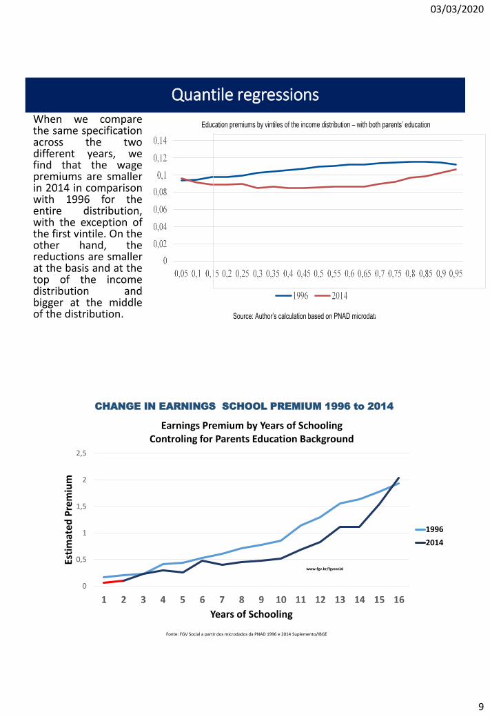
Quantile regressionsWhen we comparethe same specificationacross the twodifferent years, wefind that the wagepremiums are smallerin 2014 in comparisonwith 1996 for theentire distribution,with the exception ofthe first vintile. On theother hand, thereductions are smallerat the basis and at thetop of the incomedistribution andbigger at the middleof the distribution.

Education premiums by vintiles of the income distribution – with both parents’ education

Source: Author’s calculation based on PNAD microdata.

Education premiums by vintiles of the income distribution – with both parents’ education

Source: Author’s calculation based on PNAD microdata.

Education premiums by vintiles of the income distribution – with both parents’ education

Source: Author’s calculation based on PNAD microdata.

CHANGE IN EARNINGS SCHOOL PREMIUM 1996 to 2014

www.fgv.br/fgvsocial

Fonte: FGV Social a partir dos microdados da PNAD 1996 e 2014 Suplemento/IBGE

0

0,5

1

1,5

2

2,5

1 2 3 4 5 6 7 8 9 10 11 12 13 14 15 16

Esti

mat

edP

rem

ium

Years of Schooling

Earnings Premium by Years of SchoolingControling for Parents Education Background

1996

2014

03/03/2020

10

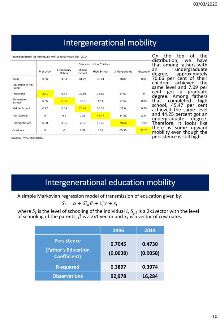
Intergenerational mobility

On the top of thedistribution, we havethat among fathers withan undergraduatedegree, approximately70.66 per cent of theirchildren achieved thesame level and 7.09 percent got a graduatedegree. Among fathersthat completed highschool, 45.47 per centachieved the same leveland 44.25 percent got anundergraduate degree.Therefore, it looks likethere is some upwardmobility even though thepersistence is still high.

Transition matrix for individuals with 15 to 59 years old - 2014

Education of the Children

Preschool Elementary

School Middle School

High School Undergraduate Graduate

Total 0.06 4.84 31.27 40.24 18.07 0.82

Education of the Father

Preschool 2.41 6.84 32.91 33.52 14.97 0

Elementary School

0.05 5.56 30.6 42.1 17.64 0.86

Middle School 0.12 0.04 20.47 56.35 21.6 0.79

High School 0 0.2 7.25 45.47 44.25 2.24

Undergraduate 0.03 0.05 2.19 19.55 70.66 7.09

Graduate 0 0 1.32 8.27 65.96 22.75

Source: PNAD microdata.

Intergenerational education mobility

A simple Markovian regression model of transmission of education given by:

𝑆𝑖 = 𝛼 + 𝑆𝑝𝑖′ 𝛽 + 𝑥𝑖

′𝛾 + 𝜀𝑖

where 𝑆𝑖 is the level of schooling of the individual 𝑖, 𝑆𝑝𝑖 is a 2x1vector with the level of schooling of the parents, 𝛽 is a 2x1 vector and 𝑥𝑖 is a vector of covariates.

1996 2014

Persistence

(Father’s Education Coefficient)

0.7045

(0.0038)

0.4730

(0.0058)

R-squared 0.3897 0.3974

Observations 92,978 16,284

03/03/2020

11

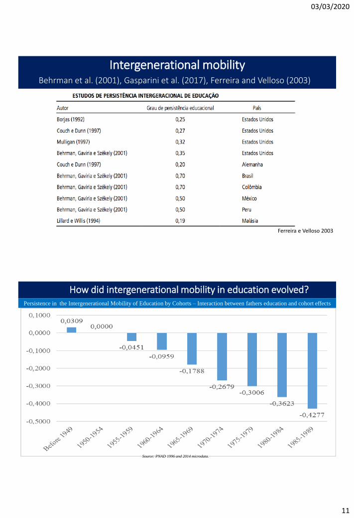
Intergenerational mobility Behrman et al. (2001), Gasparini et al. (2017), Ferreira and Velloso (2003)

Ferreira e Velloso 2003

How did intergenerational mobility in education evolved?Persistence in the Intergenerational Mobility of Education by Cohorts – Interaction between fathers education and cohort effects

Source: PNAD 1996 and 2014 microdata.

03/03/2020

12

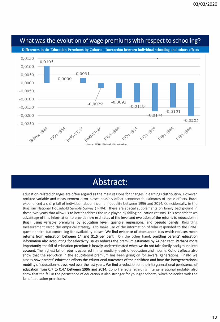
What was the evolution of wage premiums with respect to schooling?

Differences in the Education Premiums by Cohorts - Interaction between individual schooling and cohort effects

.

Source: PNAD 1996 and 2014 microdata.

Education-related changes are often argued as the main reasons for changes in earnings distribution. However,omitted variable and measurement error biases possibly affect econometric estimates of these effects. Brazilexperienced a sharp fall of individual labour income inequality between 1996 and 2014. Coincidentally, in theBrazilian National Household Sample Survey ( PNAD) there are special supplements on family background inthese two years that allow us to better address the role played by falling education returns. This research takesadvantage of this information to provide new estimates of the level and evolution of the returns to education inBrazil using variable premiums by education level, quantile regressions, and pseudo panels. Regardingmeasurement error, the empirical strategy is to make use of the information of who responded to the PNADquestionnaire but controlling for availability biases. We find evidence of attenuation bias which reduces meanreturns from education between 14 and 31.5 per cent. On the other hand, omitting parents’ educationinformation also accounting for selectivity issues reduces the premium estimates by 24 per cent. Perhaps moreimportantly, the fall of education premium is heavily underestimated when we do not take family background intoaccount. The highest fall of returns occurred in intermediary levels of education and income. Cohort effects alsoshow that the reduction in the educational premium has been going on for several generations. Finally, weassess how parents’ education affects the educational outcomes of their children and how the intergenerationalmobility of education has evolved over the last years. We find a reduction on the intergenerational persistence ofeducation from 0.7 to 0.47 between 1996 and 2014. Cohort effects regarding intergenerational mobility alsoshow that the fall in the persistence of education is also stronger for younger cohorts, which coincides with thefall of education premiums.

Abstract:

03/03/2020

13

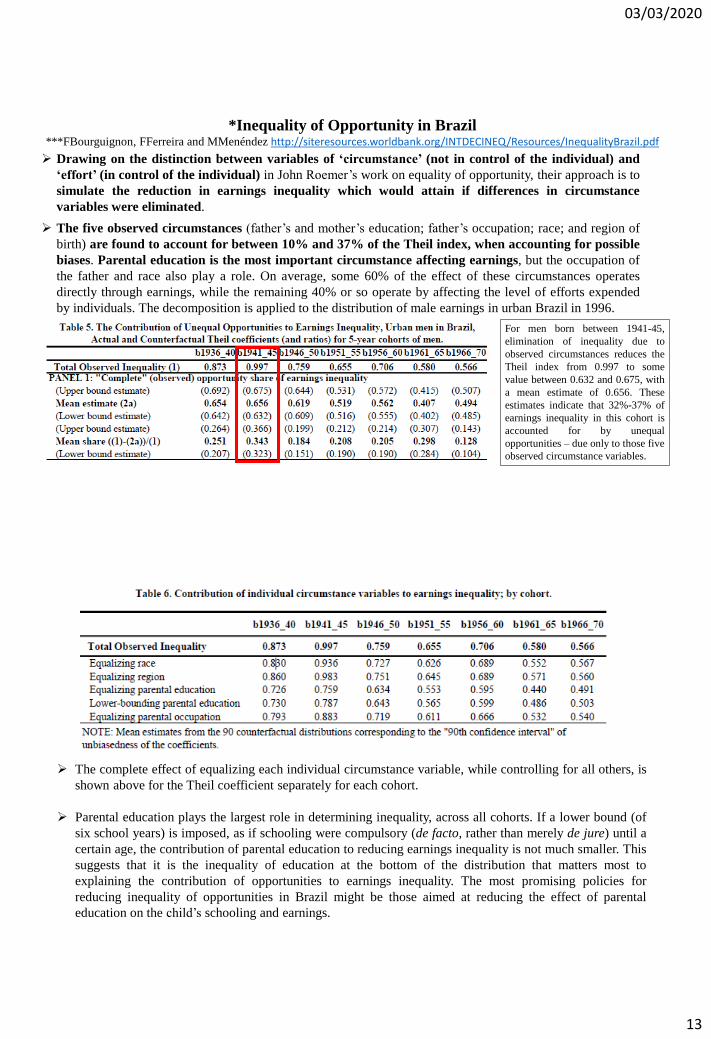
*Inequality of Opportunity in Brazil***FBourguignon, FFerreira and MMenéndez http://siteresources.worldbank.org/INTDECINEQ/Resources/InequalityBrazil.pdf

Drawing on the distinction between variables of ‘circumstance’ (not in control of the individual) and

‘effort’ (in control of the individual) in John Roemer’s work on equality of opportunity, their approach is to

simulate the reduction in earnings inequality which would attain if differences in circumstance

variables were eliminated.

The five observed circumstances (father’s and mother’s education; father’s occupation; race; and region of

birth) are found to account for between 10% and 37% of the Theil index, when accounting for possible

biases. Parental education is the most important circumstance affecting earnings, but the occupation of

the father and race also play a role. On average, some 60% of the effect of these circumstances operates

directly through earnings, while the remaining 40% or so operate by affecting the level of efforts expended

by individuals. The decomposition is applied to the distribution of male earnings in urban Brazil in 1996.

For men born between 1941-45,

elimination of inequality due to

observed circumstances reduces the

Theil index from 0.997 to some

value between 0.632 and 0.675, with

a mean estimate of 0.656. These

estimates indicate that 32%-37% of

earnings inequality in this cohort is

accounted for by unequal

opportunities – due only to those five

observed circumstance variables.

The complete effect of equalizing each individual circumstance variable, while controlling for all others, is

shown above for the Theil coefficient separately for each cohort.

Parental education plays the largest role in determining inequality, across all cohorts. If a lower bound (of

six school years) is imposed, as if schooling were compulsory (de facto, rather than merely de jure) until a

certain age, the contribution of parental education to reducing earnings inequality is not much smaller. This

suggests that it is the inequality of education at the bottom of the distribution that matters most to

explaining the contribution of opportunities to earnings inequality. The most promising policies for

reducing inequality of opportunities in Brazil might be those aimed at reducing the effect of parental

education on the child’s schooling and earnings.