Income Shocks and Suicides:

Causal Evidence From Indonesia∗

Cornelius Christian, Lukas Hensel, and Christopher Roth

July 31, 2018

Abstract

We examine how income shocks affect the suicide rate in Indonesia. We use both

a randomized conditional cash transfer experiment, and a difference-in-differences

approach exploiting the cash transfer’s nation-wide roll-out. We find that the cash

transfer reduced yearly suicides by 0.36 per 100,000 people, corresponding to an 18

percent decrease. Agricultural productivity shocks also causally affect suicide rates.

Moreover, the cash transfer program reduces the causal impact of the agricultural

productivity shocks, suggesting an important role for policy interventions. Finally,

we provide evidence for a psychological mechanism by showing that agricultural

productivity shocks affect depression.

Keywords: Economic Shocks, Mental Health, Suicides, Cash Transfer.

JEL classification: D12, C21, I38.

∗ Cornelius Christian, Department of Economics, Brock University; e-mail: cchris-

tian2@brocku.ca; Lukas Hensel, Department of Economics, University of Oxford; e-mail:

Lukas.Hensel@economics.ox.ac.uk. Christopher Roth, Institute on Behavior and Inequality; e-

mail: Chris.Roth@briq-institute.org. We thank the co-editor, Rohini Pande, and four anonymous

referees for very useful suggestions. We would like to thank Damian Clarke, Jon de Quidt, Esther

Duflo, Jan Emanuelle De Neve, James Fenske, Thomas Graeber, Alexis Grigorieff, Ingar Haaland,

Johannes Haushofer, Johannes Hermle, Matt Lowe, Climent Quintana-Domeque, Simon Quinn, Timo

Reinelt, Marc Witte, and Johannes Wohlfart for comments and help. We also thank various confer-

ence and seminar participants for comments on the paper. We are grateful to Sudarno Sumarto, Jan

Priebe, Matthew Gudgeon, the National Team for the Acceleration of poverty reduction (TNP2K)

and the World Bank for sharing several sources of data. Lukas Hensel gratefully acknowledges

financial support by the Economic and Social Research Council (ESRC). Any errors are our own.

1

1 Introduction

Suicide is a pressing public health concern, causing 800,000 deaths per year globally

(WHO, 2014). Suicidal behavior is one of the leading causes of death for people with

severe mental illness (Hawton et al., 2013). While the effects of economic conditions

on mental health and depression are well-established (Baird et al., 2011; Haushofer and

Shapiro, 2016), little is known about the causal effect of economic well-being on suicidal

behavior. More specifically, no causal evidence exists that examines whether positive

income shocks, such as poverty alleviation programs, can decrease suicides.

It is difficult to credibly quantify the impact of improved economic well-being and,

in particular, poverty alleviation programs on suicides. First, it is challenging to find

suicide data at sufficiently low levels of geographic disaggregation for statistical power.

Second, the timing and geographic placement of large government programs is usually

endogenous, and even if small-scale programs demonstrate causality, external validity

concerns predominate (Allcott, 2015; Deaton, 2010).

Our data and empirical setting address these difficulties. We focus on Indonesia, the

world’s fourth most populous country. We leverage unique Indonesian village-level census

data from 2000 to 2014, and use several identification strategies to examine the causal

effect of income shocks: First, we use a conditional cash transfer program, Program

Keluarga Harapan (PKH), which provides households with yearly cash transfers worth

about 10% of their pre-treatment annual consumption over six years. Using a difference-

in-differences specification, we estimate the effect of the program’s nationwide roll-out.

The program targeted subdistricts with high poverty, sufficient supply-side institutions

(health and educational institutions), and was launched in 2007 when it covered 13% of

Indonesian subdistricts in seven provinces and was strongly expanded, reaching 57% of

subdistricts in all 33 provinces in 2013. We also analyze a randomized controlled trial

of the same program. Second, we exploit plausibly exogenous agricultural productivity

shocks using rainfall variation and we examine whether the effects of the cash transfer

vary systematically with these agricultural productivity shocks.

2

We establish several novel facts on the relationship between economic well-being and

suicides. Our first finding is that both the cash transfer’s roll-out and the randomized

cash transfer cause a large reduction in suicides. Our preferred specification suggests

that an average per-capita transfer of 22.45 USD targeted at the poorest 10 percent of

households causes a decrease by approximately 0.36 suicides per 100,000 population per

year. This corresponds to a reduction of the suicide rate by approximately 18 percent

relative to the mean suicide rate (in 2011 and 2014) of 2 suicides per 100,000 in control

subdistricts. Second, we show that agricultural productivity shocks, proxied by rainfall,

significantly affect the incidence of suicide. A one-standard deviation increase in rain-

fall increases yearly per-capita consumption by 21.6 USD and decreases the number of

suicides per 100,000 inhabitants by approximately 0.08, corresponding to a reduction by

6 percent relative to the average suicide rate in Indonesia between 2000 and 2014. For

the subsamples affected by the income shocks, our calculations suggest that per-dollar

effects on suicides identified using rainfall are significantly smaller than those from cash

transfers. Third, we establish that cash transfers lower suicides most strongly in sub-

districts experiencing negative agricultural productivity shocks. This is consistent with

social welfare programs mitigating the adverse effects of negative economic shocks.

Finally, we provide evidence that economic hardship may ignite suicidal behavior by

affecting people’s mental health. The medical literature suggests that stress (Mann et al.,

1999) and mental illness, such as depression, are major causes for suicides (Boldrini and

Mann, 2015). We use panel data from the Indonesian Family Life Survey to show that

agricultural productivity shocks causally affect farmers’ mental health. A one-standard

deviation increase in subdistrict level rainfall increases consumption by approximately

seven percent, and reduces depression by 0.12 of a standard deviation. Moreover, the

relationship between rainfall and depression is absent for non-farmers, indicating that

the effects of rainfall operate through an economic channel.

We contribute to the literature on how economic and social circumstances affect sui-

cides (Becker and Woessmann, 2018; Campaniello et al., 2017; Cutler et al., 2001; Daly

et al., 2013; Ludwig et al., 2009; Stevenson and Wolfers, 2006). Concurrent work by

3

Carleton (2017) shows that, across Indian states, for temperatures above 20◦C, a 1◦C rise

causes roughly 70 suicides per day, particularly during the agricultural growing season.1

Our evidence supports the view that cash transfer programs’ positive effects on recipi-

ents’ mental health (Haushofer and Shapiro, 2016) outweigh negative spillovers of such

programs (Baird et al., 2013).

Moreover, our paper contributes to the literature on poverty, income shocks, and men-

tal health, the latter of which is usually measured through self-reported scales (Adhvaryu

et al., forthcoming; Apouey and Clark, 2015; Baicker et al., 2013; Cesarini et al., 2015;

Das et al., 2007; Devoto et al., 2012; Friedman and Thomas, 2009; Gardner and Oswald,

2007; Kling et al., 2007; Kuhn et al., 2011; Persson and Rossin-Slater, 2018; Stillman et

al., 2009). In particular, previous papers examine the effects of randomized cash transfers

on mental health through survey questions (Baird et al., 2013; Paxson and Schady, 2007).

An exception is Haushofer and Shapiro (2016), who show that large, unconditional cash

transfers can reduce cortisol levels, consistent with self-reported reductions in stress.

Our study advances the literature on poverty and mental health in three ways. First,

we provide the first causal evidence on whether positive income shocks, and in particular

government poverty alleviation programs, reduce suicides. Second, unlike previous evi-

dence on income shocks and mental health which mostly relies on small-scale experiments,

we use both a large-scale nation-wide roll-out of a conditional cash transfer program and

a randomized evaluation of the same program. Finally, we provide the first evidence on

the interaction between social welfare programs and agricultural productivity shocks on

mental health, underlining the potential of government programs to alleviate negative

consequences of adverse economic shocks.

We proceed as follows. In Section 2, we outline a conceptual framework, describe the

data, and the cash transfer program. In Section 3, we present our identification strategies,

and describe our results using both the cash transfer and agricultural productivity shocks.

In Section 4, we examine mechanisms underlying our estimated treatment effects by

1 There is also correlational evidence highlighting that recessions increase suicides (Barr et al., 2012;

Chang et al., 2013; Reeves et al., 2012).

4

employing microdata on depression. In Section 5, we discuss effect sizes and we conclude

in Section 6.

2 Conceptual Framework, Context, and Data

In this Section we describe the conceptual framework, the main features of the conditional

cash transfer program, the suicide data, and the construction of the subdistrict panel.

Finally, we report some basic descriptive statistics about Indonesian suicide rates.

2.1 Conceptual Framework

Related literature What are the theoretical links between economic well-being and

suicides? Previous psychiatric disorders are the most important factor in explaining death

by suicide; 90% of those who commit suicides had such a disorder (Cavanagh et al., 2003).

Hawton et al. (2013) claim that specific mental health problems, like depression, are

mainly responsible for the decision to commit suicides. Poverty and negative economic

shocks are, in turn, associated with mental health disorders and depression in particular

(Haushofer and Fehr, 2014; McInerney et al., 2013; Schilbach et al., 2016). Negative life

experiences, such as loss of income and job loss, have also been identified as risk factors

for suicide.2

Stress is a likely mechanism at play as suicide risk is correlated with abnormal cortisol

concentrations, and a maladaptive cortisol response to stress (O’Connor and Nock, 2014).

This is line with psychological models of suicide that emphasize that pre-existing medical

conditions lead to suicidal tendencies when compounded by stress (Mann et al., 1999).3

2 In addition, there is a literature emphasizing that suicides can be contagious, i.e. that the social

environment plays an important role (Hedstrom et al., 2008). There are also literatures that examine

how genes (Roy, 1992), social isolation (Appleby et al., 1999), and personality traits (Bluml et al.,

2013) affect people’s tendency to commit suicides.3 Joiner (2005) puts forward an interpersonal theory of suicide, which posits that the coexistence of

high feelings of burdensomeness, low levels of belongingness, and the belief that these conditions are

5

The main object of interest in this paper is to understand how economic shocks affect

the suicide rate. Positive economic shocks could affect the suicide rate directly by miti-

gating the consequences of negative live experiences or through improvements in mental

health. In Section 4, we provide suggestive evidence in support of mental health as a

channel by analyzing the relationship between economic shocks and depression.

Functional Form Our data and setting allow us to provide evidence on the functional

form of the relationship between income and suicides. Models of reference-dependent

preferences predict declining effects of permanent income shocks over time as individuals’

reference points adapt to the income level.4 Indeed, previous evidence suggests that the

effects of permanent improvements in economic circumstances on self-reported mental

well-being decline over time as individuals adapt to their new economic situation (e.g.

Frederick and Loewenstein, 1999; Galiani et al., forthcoming). We test the predictions

of models of reference-dependence by analyzing the dynamic treatment effects over the

program duration of six years.

Are the marginal returns of income on mental health and suicide decreasing in income?

To address this question, we shed light on the functional form between the suicide rate and

income. If the relationship between the suicide rate and income is concave (convex) the

impact of a positive income shock should be larger (smaller) if the recipients of the shock

are poorer to begin with. If the relationship is linear there should be no heterogeneity by

initial poverty levels. We test between different functional forms by analyzing treatment

heterogeneity of the cash transfer program by the extent of initial poverty as proxied by

agricultural productivity shocks and pre-treatment per-capita household consumption.

Types of Income Shocks Different types of income shocks may have different quan-

titative impacts on the suicide rate. The effect of an income shock likely depends on

hopeless to change, lead to the development of suicidal desires. Finally, social isolation and lack of

social support consistently predict suicide risk (Appleby et al., 1999).4 Models in which the reference point fully adapts after one period predict that there is a fall in suicides

only in the first year of a permanent income shock and no effects thereafter.

6

its effect on expected lifetime income and the uncertainty about lifetime income, that is

its current consumption value. Therefore, predictable and regular cash transfers should

have larger per-dollar impacts on the suicide rate than unpredictable agricultural income

shocks, a prediction that we test in this paper.

2.2 The Conditional Cash Transfer Program

We use the Program Keluarga Harapan (PKH) conditional cash transfer program to ana-

lyze the impact on suicide rates (Banerjee et al., 2017; Cahyadi et al., 2018; World Bank,

2011). A pilot version of the PKH was introduced in 2007 for 600,000 households and

the program was then expanded to cover 5.2 million households in 2014 with a target

of 10 million recipients in 2018 (World Bank, 2011). The introduction of the PKH pro-

gram was part of a wider effort to reform the Indonesian social safety system. In 2005

the Indonesian government removed universal fuel subsidies. To alleviate the immediate

inflationary shock for poor and near-poor households, the Indonesian government intro-

duced an unconditional cash transfer program covering 19 million households from 2005 to

2006. Furthermore, with the end of fuel subsidies already existing large-scale social assis-

tance programs such as rice subsidies for poor households (Beras untuk Rakyat Miskin,

or Raskin) and subsidized health insurance for the poor (Asuransi Kesehatan Miskin,

Askeskin) were expanded. The PKH program was introduced in 2007 after the uncondi-

tional cash transfer ended to provide more targeted assistance to the poorest households

(World Bank, 2012).5

PKH was designed to improve poor households’ health and education through a cash

transfer, conditional on their participation in health and education services (World Bank,

2011). The intervention’s size is substantial: households received between 39 and 220 US

dollars per year. The average received amount constituted about 10% of pre-PKH yearly

household expenditure (80.82 US dollars at 2005 prices) between 2007 and 2014 (World

5 PKH’s coverage is significantly below of that of the other social benefit programs, but due to its

targeted nature the World Bank considers it one of the most effective Indonesian social assistance

programs (World Bank, 2017).

7

Bank, 2011, 2017). Households are part of the PKH program for up to six years.

The total cost of the PKH program from 2007 to 2014 was around 716 million USD at

2005 prices. In total there were 7.6 million household-years of cash transfer such that the

average expenditure per household-year was 94 USD (World Bank, 2017). According to

the 2011 village census, the average household size in Indonesia in 2011 was 3.6 individuals

which implies an expenditure of 26.11 USD per treated individual and year. Subtracting

administrative overhead households received, on average, 22.45 USD per capita.

Geographic Roll-Out of Program In Section 3.1 we exploit the roll-out of the PKH

program for identification. The program was first implemented as a pilot program in

2007 in seven provinces: West Java, East Java, North Sulawesi, Gorontalo, East Nusa

Tenggara (NTT), West Sumatra and DKI Jakarta. These provinces are quite diverse in

terms of their poverty levels, and other economic and geographic characteristics. Because

the program’s focus is on poverty alleviation, upper income quintile districts were initially

excluded from PKH eligibility, based on an index considering poverty rates, malnutrition

and schooling records.6 The 2007 roll-out of the program was randomized among selected

eligible districts.

From 2008 to 2010, the program maintained its pilot status but was further rolled

out in the following provinces: Nanggroe Aceh Darussalam, North Sumatra, Banten,

South Kalimanten, West Nusa Tenggara, and the Yogyakarta Special Region. From 2010

onward, the Secretariat of the National Team for the Acceleration of Poverty Reduc-

tion (TNP2K), at the Office of the Vice-President, has been promoting the nation-wide

expansion of PKH leading to all Indonesian provinces being covered by 2012. Of the sub-

districts included in our analysis, the PKH program covered about 13% of all Indonesian

subdistricts when it started in 2007. By 2013, 57% of all Indonesian subdistricts in our

sample were in receipt of the program.

6 Districts receiving the rural community-driven development project were eligible for the community

cash transfer program (PNPM Generasi), and therefore were ineligible for the PKH program during

the pilot operation.

8

At the macro level, targets for overall recipient numbers and total expenditure were

set at the national level which determined the overall speed of the roll-out. At the micro

level, target subdistricts were determined in cooperation with provincial and district

governments who made recommendations. The final decisions took into account three

main factors: subdistrict poverty levels, existence of the necessary supply-side institutions

(e.g. educational institutions and health centers), and the willingness of local partners to

cooperate.

Randomized Experiment In Section 3.2 we use a subsample of subdistricts in which

the treatment status was randomly assigned and which formed the basis for the World

Bank’s evaluation of the program (World Bank, 2011). A total of 736 subdistricts were in-

cluded in the sample, with 438 subdistricts randomized to the treatment group (Cahyadi

et al., 2018). Out of these, we observe treatment assignment for 360 subdistricts that

were randomly chosen for data collection by the World Bank (180 treatment, 180 con-

trol). Political pressures and a consequent unexpected program expansion in East Java

resulted in deviations of the realized allocation from the intended one.7 To deal with this

contamination, we use the original treatment assignment to measure the conditional cash

transfer program’s impact on suicide.

Beneficiary Selection At the subdistrict level, the cash transfer program was offered

to a list of eligible households that satisfied both certain demographic as well as cer-

tain economic requirements. A 2005 census from a national unconditional cash transfer

program was initially used to construct the list of eligible households per village. Ap-

proximately 30-40 percent of beneficiaries from the unconditional cash transfer program

7 In particular, 37 out of the 360 subdistricts that were supposed to be part of the control group received

PKH funds before 2011. Moreover, for a very few subdistricts, the program started in 2008 or 2009

rather than in 2007. Bias might result from this contamination, since it is possible that unobserved

factors within the contaminated subdistricts also affected household responses. The contamination

increased further leading to 30 percent of control subdistricts receiving the program by 2014.

9

were not included in the list of eligible households.8 Based on this list of households, de-

mographic data was used to identify eligible households that fulfilled one of the following

program criteria: (i) households with pregnant and/or lactating women; (ii) households

with children aged 0-15 years; (iii) households with children aged 16-18 years who have

not yet completed 9 years of basic education. However, only the subset of eligible house-

holds with the lowest predicted consumption were included in the program. In the end,

approximately 10% of households received the program. The classification was based on

proxy-means tests of all households on the list of eligibles to identify program beneficia-

ries. The proxy-means tests consisted of 29 variables, including housing characteristics,

education levels, sources of fuel, employment information, and access to health and edu-

cation services.

2.3 Data

We use the censuses of all Indonesian villages (PODES) from 2000, 2003, 2005, 2011, and

2014 to examine the PKH program’s effect on suicide rates. The PODES data covers all

80,000 villages in Indonesia. In the village census, village heads report village character-

istics, such as population size, the presence of health and educational institutions, and

data on the percentage of farmers.

Outcome Definitions The census contains data on suicides at the village level. In

2000, 2003 and 2005 the village head was asked whether any suicide occurred in their

village in the previous year. In 2011 village heads were asked about the number of suicides

committed in the last year. Finally, in 2014 the PODES survey asked for the number

of suicides and suicide attempts in the village last year. Village level population data is

available from 2000 to 2011, but not for 2014. To obtain population data for 2014, we

extrapolate population size using a liner trend from the years 2005 and 2011 to 2014 at

the subdistrict level.

8 Statistics Indonesia also conducted additional interviews in targeted subdistricts to identify newly

poor households, in an attempt to minimize exclusion errors.

10

We use the PODES census data to construct our main outcome measure of interest:

the number of suicides per 100,000 inhabitants at the subdistrict level. For the years 2000,

2003 and 2005 (all prior to the cash transfer program), we use the number of villages with

at least one suicide per 100,000 inhabitants as a proxy for the actual suicide rate. For

the PODES 2011 data we directly use the number of suicides per 100,000 inhabitants at

the subdistrict level. Lastly, we define the suicide rate in 2014 as the number of suicides

and suicide attempts per 100,000 inhabitants.

We also construct a measure of the suicide rate whose definition does not vary across

years (except for 2014 when the question included suicide attempts). Specifically, we

extrapolate the expected suicide rate from the subdistrict mean of village level occurrences

of at least one suicide. We rely on two assumptions for this exercise: First, we assume

that suicides are Poisson-distributed. Second, we assume that suicides in all villages of the

same subdistrict are independent and have the same Poisson parameter λ. Under these

assumptions we can use the mean incidence of at least one suicide (s) to calculate the

expected number of suicides Ev(s) in a given village as Ev(s) = − ln (1− s).9 To calculate

the expected number of suicides at the subdistrict level we multiply Ev(s) by the number

of villages in a subdistrict. We validate this measure with data on the actual number

of suicides in the years 2011 and 2014 and find a correlation of ρ = 0.95. Moreover, in

Section 3.4 we show that our results are robust to using different outcome measures.

According to the WHO Health Data repository the age-standardized suicide rate in

Indonesia stood at around 3 per 100,000 in 2015. This seems relatively well-aligned with

our data where we find mean raw suicide rates of approximately 2 per 100,000 at the

subdistrict level in 2011 and 2014, respectively.10

9 This is derived from the cumulative distribution function of the Poisson Distribution: CDF (k) =

e−λ∑bkci=0

λi

i! . We observe the fraction of villages with zero reported suicides, which gives a subdistrict

specific estimate of CDF (0). Expressed as fraction of villages with at least one suicide we get:

CDF (0) = 1 − s. Using the functional form of the Poisson distribution we obtain Ev(s) = λ =

− ln (1− s). There is one subdistrict in 2014 where all villages have at least one suicide or suicide

attempt. For this observation we use the average subdistrict λ over the preceding four years.10 The slight discrepancy between those numbers can be explained by the fact that the WHO estimates

11

Indonesia has low suicide rates from an international perspective. In a WHO world-

wide ranking of all nations by suicide rates, Indonesia ranked 173 out of 183 nations. This

low baseline suicide rate could imply stronger social norms against suicides in Indonesia.

These norms might not only affect the level of the suicide rate, but also the elasticity of

suicides with respect to economic shocks. However, it is theoretically unclear how these

norms would affect the relationship between the suicide rate and economic circumstances.

On the one hand, decisions to commit suicide might be more marginal than in other

countries, that is a small improvement in economic circumstances could prevent more

suicides. On the other hand, it is possible that because of the strong stigma non-economic

factors play a more important role for suicides in Indonesia.

Subdistrict Panel Construction Since our key identifying variation is at the sub-

district level, we aggregate our village panel at the subdistrict level, and collapse our

observations at the subdistrict boundaries from 2000. We use 2000 subdistrict bound-

aries as 2000 is the first year for which suicide data is available.11 For practical reasons

we construct our panel at the subdistrict level as the number of administrative units in

Indonesia substantially increased over time.12 In the experimental sample there are 314

subdistricts according to 2000 boundary definitions. In our analysis we only make use of

310 subdistricts for which we can construct a cross-walk between 2000 and 2014. For the

roll-out of the program and the analysis of agricultural productivity shocks (presented in

are model-based and only partially take into account micro-data on suicides in Indonesia.11 We use 2000 borders to provide a consistent interpretation of coefficients for all our subdistrict level

specifications. Furthermore, using subdistrict border definitions from after 2000 would complicate

both the presentation of pre-trends and the analysis of interactions between agricultural productivity

shocks and cash transfers (presented in Section 3.1 and 3.6). We show that our results are robust to

using the 2006 subdistrict borders (Tables A.8 and A.14).12 Decentralization reforms beginning from 1998 significantly increased the proliferation of administrative

units. For example, the number of districts increased from 302 in 1999 to more than 500 in 2014 (Bazzi

and Gudgeon, 2018). The number of subdistricts increased from about 3000 in the late 1990s to

approximately 7000 in 2014. Constructing a cross-walk at the village level is particularly challenging

and would necessarily result in a large number of incorrect matches over time. This in turn would

substantially increase measurement error of outcomes.

12

Section 3.4) we employ the universe of Indonesian subdistricts for which we could con-

struct a consistent panel between 2000 and 2014. We were able to construct such a panel

for 3138 out of all 3928 subdistricts according to 2000 boundary definitions. The panel’s

construction was based on a subdistrict-level crosswalk for the time period of 2000 to

2014. Owing to the subdistrict-splits, there are 1485 cases in which a subdistrict split

from 2000 to 2014. If only a part of the 2000 subdistrict received the cash transfer in

a given year, we define the treatment indicator as the fraction of new subdistricts re-

ceiving the PKH program. When we drop the observations with partially treated origin

subdistricts our estimated treatment effects barely change (see Tables A.6 and A.12).

Descriptives and Correlates of Suicide Rates Table 1 displays descriptive statis-

tics at the subdistrict level from the PODES 2005 data, before the cash transfer was

implemented. On average, a subdistrict consists of 17.6 villages and has a population of

approximately 56,000. Most subdistricts are relatively rural, with on average 74% of vil-

lages classified as rural and 56% of the population working as farmers. Thus, agricultural

productivity shocks are likely to affect large parts of the population. The RCT sample is

more rural than the average, but otherwise is similar to non-RCT subdistricts.

[Insert Table 1]

Second, we exploit baseline data from the 2005 census to characterize the correlates

of suicides. We find a strong economic gradient in suicide rates. Subdistricts in districts

with a 10% larger share of the households below the poverty line have, on average, a

0.142 higher suicide rate per 100,000 people (see Column 1 of Table A.1 in the Online

Appendix). The same pattern is apparent when we consider per capita expenditure at

the district level. Moreover, the share of farmers at the subdistrict level is strongly

positively correlated with suicide rates. The share of farmers at the subdistrict level

remains significantly correlated with suicide rates after controlling for local crime rates,

and health, education, and social institutions.13 Table A.1 also reveals that crime per

13 Since the share of farmer variable is available at the subdistrict level, this may explain why it remains

statistically significant, while per capita expenditure and fraction poor which are measured at the

13

capita is weakly positively related to suicide incidence, but that social organizations per

capita and educational institutions per capita are not correlated with suicide rates.14

Finally, we observe an increase in the occurrence of any suicide in subdistricts over

time. Specifically, the incidence of at least one suicide at the subdistrict level increased

from 21 percent in 2000 to 45 percent in 2005 and 52 percent in 2011 and 2014.15,16

3 Main Results

In this Section, we first present evidence from the difference-in-differences approach using

the population-wide roll-out of the cash transfer program. Then we show results of a

randomized controlled trial of the same program. Thereafter, we examine the dynamics

of treatment effects, and assess the robustness of our findings. Finally, we study how

agricultural productivity shocks affect suicide rates, and examine how they interact with

the roll-out of the cash transfer program.

3.1 Nation-Wide Program Roll-Out

We provide evidence that the PKH conditional cash transfer program substantially de-

creased the suicide rate using a difference-in-differences approach exploiting the nation-

wide roll-out of the program. For our main specification we use suicide data from the

census of villages from 2005, 2011, and 2014, but we also employ data from 2000 and 2003

to assess robustness and pre-trends. Our dependent variable is the number of suicides

district level, become statistically insignificant.14 We find that health institutions per capita are positively correlated with suicide rates, consistent with

the government targeting health care provision to more needy subdistricts.15 The increase in reported suicides between 2000 and 2005 could be the result of shifting norms around

suicides, potentially affecting the willingness to report suicides by the village chiefs. However, such a

shift of norms can only explain our results if it occurred differentially in subdistricts with and without

the cash transfer program and in subdistricts with and without agricultural productivity shocks.16 Comparing other measures of suicides over time is complicated by changing survey questions and

changes in the number of villages per subdistrict.

14

per 100,000 individuals (yst) in subdistrict s and at time t.

To estimate treatment effects, we include subdistrict fixed effects (αs), time fixed

effects (φt), and a treatment indicator, Treatst, taking value one when a subdistrict started

receiving the program.17 Even though the identifying variation is at the subdistrict

level, we cluster standard errors at the district level, as the roll-out of the program was

correlated at the district level. We estimate all of our main specifications with OLS and

employ population weights from 2005.18 Our specification of interest is:

yst = δ1Treatst + αs + φt + εst (1)

Our main coefficient of interest is δ1, which provides us with the treatment effect for the

subdistricts that had started receiving the program at the time of the data collection.

Column 1 of Table 2 shows that receiving the cash transfer program of on average 22.45

USD per year reduces the number of suicides per 100,000 inhabitants by 0.36. This

corresponds to a reduction by approximately 18 percent relative to the control mean in

2011 and 2014. Our estimates remain economically and statistically significant when

(i) clustering errors at the subdistrict level (Column 2), (ii) excluding the sample of

subdistricts with randomized treatment assignment employed in Section 3.2 (Column 3),

including all pre-treatment periods (Column 4) and including subdistrict specific time

trends (Column 5). Column 6 displays the treatment effects that give equal weight to

the subdistricts regardless of their population size in 2005. This reveals an estimate of

-0.591 suicides per 100,000 people, suggesting that the suicide reductions are larger in

subdistricts with smaller population sizes.19

17 For subdistricts that split up over time, the treatment variable indicates the fraction of subdistricts

(based on the 2000 boundary definitions) that receive the treatment.18 We use population weights since the welfare relevant metric of interest are changes in the overall

Indonesian suicide rate and not the average subdistrict suicide rate. Furthermore, the suicide rate is

measured with less error in larger subdistricts which increases the precision of our estimates.19 Our results are also robust to using district fixed effects instead of subdistrict fixed effects, controlling

for district trends, including controls in a specification without subdistrict fixed effects, and allowing

for differential trends by baseline covariates (Table A.9).

15

[Insert Table 2]

A key assumption underlying the difference-in-differences approach is that treatment

and control subdistricts are on parallel trends. Figure 1 provides evidence supportive

of the common trend assumption.20 It displays pre-trends relative to the timing of the

introduction of the conditional cash transfer program by treatment wave. Differences in

the first period before the treatment are normalized to zero. The displayed coefficients

are the difference-in-differences treatment effect estimates compared to subdistricts that

had not received the PKH program until 2013. Moreover, as shown above, the effects

remain both economically and statistically significant after controlling for subdistrict-

specific trends. All in all we find consistently large negative and significant effects across

a series of specifications. While we have provided evidence in support of the parallel-trend

assumption, there is no formal test of the validity of this identification assumption.

[Insert Figure 1]

3.2 Randomized Controlled Trial

In this subsection, we use a subset of subdistricts in which the treatment was randomly

assigned to test whether the experimental treatment effect estimates are in line with the

non-experimental roll-out analysis from the previous section.

Balance As a first step, we test whether the treatment and control group are balanced in

terms of observables. Let Ts denote the PKH program’s original allocation, where Ts = 1

if the subdistrict was randomly assigned to receive the program, and Ts = 0 otherwise.

We consider whether baseline balance holds for the original treatment assignment by

comparing means and clustering standard errors at the subdistrict level. In Table A.2,

20 We also provide further analysis consistent with parallel trends. Figure A.1 displays the evolution

of mean suicide rates over time. Table A.3 shows that pre-trends are uncorrelated with timing of

entry (Column 1) and that the level of the suicide rate in the period before a subdistrict received the

program does not drive the treatment effects (Column 2).

16

we provide evidence of baseline balance on a set of observables. We cannot reject the null

hypothesis of global balance (p = 0.57).

Results We estimate treatment effects using the randomized assignment of the cash

transfer program, clustering standard errors at the subdistrict level and weighting obser-

vations by population size in 2005.21 Despite the randomization of cash transfers at the

subdistrict level, we find some evidence that treated subdistricts were on an upward trend

compared to control subdistricts (Figure A.4) and some gap in the suicide rate before

the program was launched (Table A.2). As a result of the common trend violation and

the slight baseline imbalance, difference-in-differences estimators might be upward biased

and a more conservative way of evaluating treatment effects is to employ an ANCOVA

and a post-estimator.

The ANCOVA specification in Column 1 of Table 3 shows that subdistricts randomly

assigned to receive the same conditional cash transfer program as in Section 3.1 have, on

average, a 0.337 lower suicide rate (about 19% of the control mean in 2011). Comparing

mean suicide rates between treatment and control subdistricts in 2011 also yields an

insignificant average decrease of 0.258 suicides per 100,000 (Column 2). While the size

of the effect is economically meaningful and of very similar magnitude to the roll-out

estimates, it is statistically insignificant. We attribute this lack of significance to low

statistical power.22

We also estimate the effect of the RCT using difference-in-differences specifications

and find mostly significant and stronger negative treatment effects (Columns 3 to 6 of

21 We do not use the 2014 census in this section. While contamination of the randomization was quite

low in 2011 (with 10 percent of subdistricts having an actual treatment status differing from the

randomly assigned one), the contamination of the program strongly increased over time. By 2014, 30

percent of control subdistricts received the program. Moreover, the cash transfer ended in 2012 and

2013 so that only a subset of subdistricts was still receiving the program during the relevant period

from PODES 2014. We discuss the long-run effects of the PKH program in Section 3.3.22 Ex-post power calculations show that we had 80% power to detect a 0.770 effect size at the five percent

level.

17

Table 3) confirming that the cash transfer program reduced suicides. However, given

the pre-trend violation and slight baseline imbalance we think that the effect sizes of the

ANCOVA and post-estimator are more credible. All in all, the results of the RCT are in

line with the roll-out results. The key difference between the two strategies is that the

results from the roll-out are much more precisely estimated as they are based on a 10

times larger sample size than the estimates from the RCT.

[Insert Table 3]

3.3 Dynamics of Treatment Effects

The cash transfer program had persistent treatment effects throughout the six-year du-

ration of the program. Figure 2 plots the evolution of the estimated treatment effect

of the PKH program on suicide rates over time. To estimate the plotted coefficients we

exploit the fact that the census data-collection happened at different points in time rel-

ative to the beginning of the treatment for different subdistricts. This means that each

point-estimate is obtained comparing a different sample of treatment and control subdis-

tricts.23 Treated subdistricts in a given period t are defined as having received the cash

transfer program exactly t before (or after) the census. For t ≥ 0 control subdistricts are

defined as subdistricts that had not received the treatment at the time of the census. For

t < 0 control subdistricts are defined as not having received the treatment t years after

the census. This also leads to differences in sample size and precision in the estimation

of treatment effects as apparent by variation in the width of confidence intervals.

A clear temporal pattern emerges from Figure 2. Similar to the roll-out analysis there

are no detectable difference between treatment and control subdistricts in the years prior

to receiving the cash transfer program. However, starting in the year subdistricts first

receive the treatment cash transfer program the suicide rate declines by about -0.3 in line

23 We do observe some treated subdistricts at two different points in time which allows us to directly

compare treatment effects over time (Table A.16). The treatment effects for the subsample of treated

subdistricts we observe twice are in line with the results from the overall sample.

18

with the aggregate analysis. The difference in the suicide rate persists throughout the

six-year duration of the cash transfer program without any obvious changes in the effect

size.24 The treatment effect also persists into year seven after the treatment potentially

suggesting a persistence beyond the receipt of the program. However, the periods are

defined in calendar years so that we cannot rule out that persistence is driven by subdis-

tricts who started receiving the program in late 2007 still receiving the program at the

time of the census data collection in early 2014.

These findings also imply that the duration of exposure to the treatment does not

affect the estimated effects of the program. To more formally test this we run a regression

in which we include a treatment indicator as well as a variable on the number of years

of treatment received by the subdistrict. Duration of receipt is not significantly related

to suicide rates, and barely affects the coefficient on whether a given subdistrict received

the program (Table A.18). All in all, we find comparable effect sizes for short-run and

medium-run effects of the program. This finding is inconsistent with a model of reference

dependence over past income levels which predicts declining effects on suicides as soon

as people’s reference point adjusts to the new income level.

[Insert Figure 2]

3.4 Robustness: Outcome Definitions

One concern with our analysis could be that the definitions of the suicide rate change

over time. We provide three pieces of evidence that demonstrate the robustness of our

results to using less rich but time-invariant measures of subdistrict suicides.

First, we employ a measure of the suicide rate using the Poisson extrapolation de-

scribed in Section 2.3. Using this extrapolated suicide rate as outcome for all years we

see the same treatment effect patterns with similar effect sizes (Columns 1 to 5 of Table

A.4 and Figures A.6 and A.7). Second, we use a version of the suicide rate based on the

24 This finding is in line with the evidence of constant and persistent effects of the PKH program on

child health, education, and the prevalence of child labor (Cahyadi et al., 2018).

19

number of villages in a given subdistrict that report at least one suicide. This is effec-

tively a truncated version of our main outcome variable. Our treatment effect estimates

with this outcome definition remain largely unchanged (Columns 6 to 10 of Table A.4).

Third, we employ a binary variable indicating whether any suicide occurred in a given

subdistrict-year. The treatment effects are qualitatively similar to our main specification

(Columns 11 to 15 of Table A.4). Our preferred specification implies that receiving the

cash transfer reduces the likelihood of at least one suicide by 6 percentage points or 12

percent. Therefore, changes in the survey structure over time do not seem to affect our

results.

Another concern could be that the cash transfer program affects migration patterns,

and thereby shapes our treatment effect estimates. To test whether these potential

changes in migration affect our results, we estimate treatment effects on two further

outcomes not subject to this bias. First, we construct the suicide rate per 100,000 inhab-

itants using 2005 population for all years. This definition of the suicide rate is unaffected

by changes in migration induced by the cash transfer. We find that with this measure

treatment effects on the suicide rate are still highly significant (Columns 1 to 5 of Ta-

ble A.5). Second, we use the number of suicides as the outcome variable.25 Again, the

treatment effect patterns remain largely unchanged. The point estimate of our preferred

specification indicates that the cash transfer program decreased the number of suicides

per subdistrict by 0.2 (Column 11 of Table A.5). This set of results suggests that changes

in migration do not drive our main results.26

25 For this analysis we stick with the definition used for our main outcome variable and use the actual

number of suicides when available. The results remain very similar when we use the number of villages

with at least one suicide as outcome (results available upon request).26 The results for the RCT are also robust to changing outcome definitions, though the results are more

noisily measured (Tables A.10 and A.11).

20

3.5 Agricultural Productivity Shocks and Suicides

Our evidence from previous sections shows that a positive economic shock, the receipt of

a conditional cash transfer, can lower suicide rates. In this section, we examine whether

agricultural productivity shocks, as measured by rainfall, also affect suicide rates.

Rainfall Analysis The rainfall analysis has at least two advantages compared to the

analysis of the cash transfer program: First, it enables us examine whether positive and

negative income shocks have symmetric effects on the incidence of suicide. Second, it

allows us to retrieve estimates with no concerns regarding differential social desirability

bias between the treatment and the control group.27

Data Our empirical strategy relies on the following two facts: First, the agricultural

sector in Indonesia is to a large extent governed by seasonal monsoon rainfall. Second,

Indonesian rainfall exhibits substantial variability within a given year across subdistricts

as well as within subdistricts over time. To examine the causal effect of agricultural

productivity shocks, we leverage the ERA-Interim Reanalysis dataset which provides

precipitation data from 1979 until 2016 on a 0.25×0.25 degree resolution (roughly a

27.5×27.5 kilometer grid at the equator). We define rainfall at the subdistrict level as

weighted average rainfall at the five grid points closest to the geometric center of the

subdistrict.28 Each grid point is weighted with the inverse of the squared distances to

the subdistrict center. Reanalysis data is based on a mix of real weather observations

(station and satellite data) and an atmospheric climate model. The main advantage of

reanalysis data is the homogeneous data quality across time and space, which alleviates

the concern of endogenous placement of weather stations. The rainfall data is matched

to the 2000 subdistrict boundaries. We use suicide data from the 2000, 2003, 2005, 2011

27 One may be concerned that village heads whose villages are in receipt of the PKH program report

more favorable outcomes, but this critique does not apply to the rainfall analysis.28 We lack coordinates for 14 subdistricts. We use average rainfall and coordinates of other subdistricts

in the same district for these subdistricts. For one district all subdistricts have missing coordinates.

For those we use province level average rainfall and coordinates.

21

and 2014 waves of the Indonesian village census. As before, our main outcome variable

of interest, yst, is the suicide rate in a given subdistrict, s at time t.

Specification and Results We follow the recommendation in Levine and Yang (2014)

and Maccini and Yang (2009) and calculate rainfall in a particular year by focusing on

rainfall in complete wet seasons (rather than in calendar years). As in Maccini and

Yang (2009), we define rainfall, zrainst, as the normalized deviation of rainfall from the

long-term mean within a given subdistrict.29 This measure of rainfall has been shown

to significantly and strongly predict rice output (Levine and Yang, 2014). In all of our

specifications we control for subdistrict level fixed effects, αs, as well as time fixed effects,

φt. As rainfall is heavily spatially correlated, we report Conley (1999) standard errors

allowing for arbitrary spatial and temporal correlation of error terms in a 100km radius

around the subdistrict center (we also report standard errors clustered at the district

level). We estimate the following equation, using 2005 population to weight the subdistrict

observations:30

yst = γ1zrainst + αs + φt + εst (2)

Table 4 provides evidence that higher rainfall significantly reduces suicides. In Col-

umn 1 we show that increases in subdistrict-rainfall by one standard deviation from the

long-run subdistrict mean lowers the suicide rate by 0.08. In Column 3 we include sub-

district trends, to rule out that differential trends can explain our findings. We find

that our results are virtually unchanged by the inclusion of trends, and if anything, be-

come somewhat stronger.31 Column 5 assesses the sensitivity of our estimates to also

29 We use rainfall data from 1979 to 2016 to construct the subdistrict specific leave-one-out long-run

means and leave-one-out long-run standard deviations. Our results are robust to constructing the

rainfall variable in different ways. As Indonesia is located around the equator, temperature is rela-

tively constant and therefore does not have effects on agricultural yields (Kleemans and Magruder,

forthcoming).30 We use 2005 population weights to make the analysis comparable to the cash transfer estimates.31 We also estimate the impact of a detrended (at the subdistrict level) measure of rainfall on the suicide

22

controlling for the first, second, and third lag of rainfall. This leaves our estimated coef-

ficients largely unaffected. Our estimated coefficients increase further both in economic

and statistical significance once we give equal weight to subdistricts, i.e. once we do not

weight by population size (see Table A.20). This most likely reflects that subdistricts with

lower population size are more strongly economically affected by agricultural productivity

shocks.

Table A.19 tests whether the relationship between positive and negative rainfall shocks

and the suicide rate is approximately symmetric. To do so we augment the above equation

by two dummy variables: posshockst, taking value one for subdistricts experiencing a

positive shock in rainfall (top one third of the standardized rainfall distribution in our

sample) and negshockst, taking value one for districts experiencing a negative shock in

rainfall (one third percent of the standardized rainfall distribution in our sample). Then

we estimate the following equation:

yst = β1zrainst + β2posshockst + β3negshockst + αs + φt + εst (3)

We find little evidence of asymmetric responses to shocks. While the absolute value of the

point estimates for β2 are slightly larger than the estimates of β3, we cannot reject that

they are of equal size. In Figure 3 we non-parametrically assess the relationship between

rainfall and suicide. To do so, we partial out time fixed effects, subdistrict fixed effects,

and subdistrict-trends from both suicide rates and the rainfall measure. Then we use the

predicted residuals from these regressions to run local polynomial regressions between

these residuals. Figure 3 highlights a strong negative relationship between rainfall and

the suicide rate, confirms our previous result that the responses to positive and negative

rainfall shocks are fairly symmetric, and that the overall relationship is approximately

linear. However, at the top end of the rainfall distribution we observe a slight flattening

of the relationship, potentially indicating a concave relationship between income and the

rate (Tables A.22 and A.23). The results are qualitatively in line with the results from the main

specification.

23

suicide rate.

3.6 Cash Transfers and Agricultural Productivity Shocks

Do the cash transfers mitigate the adverse effects of agricultural productivity shocks on

suicides? If economic hardship caused by negative economic shocks affects suicide rates,

then we would expect cash transfers to more strongly reduce suicide rates in the face

of negative economic shocks. We test whether there are significant interactions between

receiving the cash transfer, Treatst, and rainfall, zrainst. We leverage the suicide data

from 2000 to 2014, and estimate the following equation, reporting Conley standard errors

and standard errors clustered at the district level:32

yst = γ1zrainst + γ2Treatst + γ3zrainst × Treatst + αs + φt + εst (4)

Our key coefficient of interest is γ3. Column 2 of Table 4 reveals that there is a significant

interaction effect, consistent with the idea that cash transfers are more (less) effective at

lowering suicides in years with lower (higher) agricultural productivity. Our estimates

imply that cash transfers lower suicides by 0.3 suicides per 100,000 inhabitants in a year

with subdistrict rainfall one standard deviations below its long-run mean, but only lower

suicides by 0.1 suicides per 100,000 inhabitants in a year with subdistrict rainfall one

standard deviations above its long-run mean.

These effects become slightly smaller and statistically insignificant, but remain eco-

nomically meaningful, once we control for subdistrict trends. This most likely reflects

the limited power for studying interaction effects after controlling for subdistrict trends.

The estimated effects of the interaction between the cash transfer and rainfall are much

stronger in specifications that do not use population weighting (see Table A.20). This

stems from the fact that rainfall more strongly impacts incomes in more rural subdis-

tricts which have a lower population size. We also analyze whether the effect of the cash

transfer separately for positive and negative rainfall shocks in Table A.21. While this

32 As in all other main specifications we use population size from 2005 to weight the observations.

24

analysis is limited by lower statistical power, the estimates suggest that the cash transfer

program reduces the effects of both positive and negative agricultural productivity shocks

symmetrically.

The observed heterogeneity in treatment effects suggests that social welfare programs

can dampen the effects of negative and positive economic shocks. Put differently, the

cash transfer program breaks the relationship between agricultural productivity shocks

and suicides.33 The finding of a positive interaction effect between rainfall and the receipt

of the cash transfer suggests that the relationship between the suicide rate and income is

concave and not linear or convex.

Further Heterogeneity Do other covariates predict heterogeneous responses to the

cash transfer program? There is no statistically significant heterogeneity by any prede-

termined characteristics (fraction of farmers, fraction poor, per capita expenditure, per

capita crimes, per capita social institutions, and per capita health institutions; see Table

A.27). However, our effective statistical power to detect statistical differences in treat-

ment effects across groups is quite limited (see the minimum detectable effect sizes in

Table A.27).

4 Mechanism

In the next section, we provide suggestive evidence in favor of depression as a channel

through which economic circumstances could affect people’s inclination to commit sui-

cides. In particular, we show that economic shocks directly affect a measure of depression,

in line with the framework in Section 2.1. Finally, we examine the importance of several

potential subdistrict-level mediators.

33 This interaction results suggest that the effects of the cash transfer are not driven by differential social

desirability bias between the treatment and the control group.

25

Economic Shocks and Depression: Micro-Evidence To provide evidence that

economic circumstances affect people’s inclination to commit suicides through changes

in mental health, we use unique individual-level data on depression from the Indonesian

Family Life Survey (IFLS). The IFLS waves 4 and 5 (in 2007 and 2014) administer a ten

question version of the CES-D depression scale (Radloff, 1997). The raw CES-D score

ranges from 0 (not depressed) to 30 (severely depressed).34 Moreover, we leverage rich

data on household expenditure available for all five waves of the IFLS (1993, 1997, 2000,

2007, and 2014).

As in Section 3.5, we exploit agricultural productivity shocks to study the effects of

economic circumstances. Specifically, we assess the effects of rainfall, zrainst, on depres-

sion, depressionist, as measured by the CES-D score and monthly per captita household

expenditure, expist, in levels and logs. Our object of interest are households with at least

one agricultural worker, the group of households whose income is most strongly depen-

dent on rainfall.35 We employ the same subdistrict-level rainfall measure as in Section

3.5, and also report both Conley standard errors and standard errors clustered at the

district level. We also include individual level fixed effects, αi, in our regression which

allows us to control for time-invariant individual-specific unobservables. Specifically, we

estimate the following equation:

yist = δ1zrainst + αi + φt + εist (5)

Table 5 shows that a one-standard deviation increase in rainfall increases monthly per

34 The literature estimates that 80 percent of suicides are committed by individuals with a CES-D score

above 9 (Cheung et al., 2007). This suggests that depression could be a key mechanism through which

economic shocks alter people’s inclination to commit suicides. Individuals who received the PKH cash

transfer in 2014, had higher depression scores in 2007 (0.14 standard deviation; see Table A.25).35 Households count as “working in agriculture” if any household member works in agriculture either in

self-employment (without permanent employees), or as a casual or family worker in any of the five

IFLS waves. There is no sector information for IFLS Wave 1. We therefore use working “in self-

employment without permanent employees” or working as “temporary worker” as proxies. The sample

is restricted to individuals observed in all 5 IFLS waves.

26

capita consumption of farmers by 40,000 Rupiah (Column 1), monthly log consumption by

6.9 percent (Column 2)36, and decreases depression by 0.12 standard deviations (Column

3). Columns 4 to 6 of Table 5 also provide evidence that the rainfall shocks operate

through an economic mechanism by showing that both depression and consumption of

non-farmers do not respond to rainfall shocks. This suggests that our estimated effects on

depression do not operate through direct effects of weather on mental health. Indeed, the

coefficients on the effects of rainfall on log consumption and mental health are statistically

different between farmers and non-farmers (p < 0.06).37 We also use the individual level

data to study heterogeneous effects of agricultural productivity shocks on depression.

We find that depression scores of individuals with higher baseline expenditure are more

strongly affected by rainfall shocks (Table A.24). This is consistent with the finding

that cash transfers more strongly reduce suicides in the presence of negative agricultural

productivity shocks and suggests a concave relationship between depression and income.

The effects are also significantly larger for women and below median age individuals.

Mediation Analysis What other factors could account for the effects of the cash

transfer program on suicide rates? The cash transfer increased recipients’ welfare by

increasing their consumption and improving their health outcomes (World Bank, 2011).

Guided by this, we examine several potential subdistrict-level mediators, including local

crime rates, health, and education institutions, and social organizations through which

the cash transfer program could lower the incidence of suicides. Therefore, we include

time-varying endogenous controls at the subdistrict level in our main specification of

interest. These controls could have been affected by the cash transfer in systematic ways

and therefore act as a channel through which our treatment effects operate. However, we

find little evidence that any subdistrict level institutions mediate our results. Indeed, the

treatment effect estimates hardly move when the potential mediators are included (Table

A.26). This mediation analysis is limited by the fact that we have to rely on subdistrict

36 A 6.9 percent increase over the median per-capita consumption across all years corresponds to ca.

18,000 Rupiahs or roughly 1.8 USD at 2005 prices.37 The difference in effects on consumption levels are marginally insignificant (p = 0.162).

27

level mediators, and points to the importance of individual level mediators.

5 Interpreting Effect Sizes

The impact of cash transfers on suicides of cash transfer recipients is quantitatively very

large if we assume no spillovers in suicides. Spillovers similar to those identified in previous

work are consistent with moderately large direct effects. Implied direct per-dollar effects

of income on suicides identified using rainfall are significantly smaller than those from

cash transfers.

Cash Transfer Program There are two main factors to consider when calculating the

size of the cash transfer program on recipients: First, there is a strong economic gradient

in the suicide rate. The correlation between the fraction of individuals classified as poor

and the suicide rate is large and positive (see Section A.2). A 10% higher share of the

poor population is, on average, associated with a 0.14 higher suicide rate in 2005 (Table

A.1). A back-of-the-envelope calculation suggests that poor individuals are 2.24 times

more likely to commit suicides than non-poor households.38 Second, there are likely two

types of spillover effects on non-treated individuals. First, there is evidence that suicides

are highly contagious (Hedstrom et al., 2008). Furthermore, the conditional cash transfer

might have positive economic spill-overs to households not receiving the PKH program

(Angelucci and De Giorgi, 2009). Thus, we would expect that reducing suicides among

PKH recipients may also decrease suicides among non-recipients. Assuming no spillovers,

our preferred treatment effect estimate (0.36 suicides per 100,000 people) implies that

the suicide rate among the poor decreased by 3.6 suicides per 100,000 or 89% of the

implied mean suicide rate. This effect size would imply that the suicide rate among PKH

recipients who received the transfer is lower than the rate among non-recipients post-

treatment. Therefore, it may be more reasonable to calculate the implied suicide rate

reduction among PKH recipients assuming that the cash transfer equalized suicide rates

38 For details for this and the following back of the envelope calculations see Section A.1.

28

between poor and non-poor households. This yields an estimate of a direct treatment

effect of 2.36 per 100,000 or 58.7% of the implied control group mean for PKH recipients

and an indirect effect of 0.12 for non-poor individuals (4.9% of the direct treatment

effect). Our estimated effect sizes of spillovers are modest compared to estimates from

the literature on suicide contagion (Hedstrom et al., 2008). We estimate that the program

prevented about 1065 suicides, i.e. one suicide for every 672,000 USD spent.

Agricultural Productivity Shocks To estimate the per-dollar effect size of agricul-

tural productivity shocks we use micro data from the Indonesian Family Life Survey. We

show that a one standard deviation change in rainfall induces a 6.9% change in monthly

per capita consumption for individuals in agricultural households (Table 5). This trans-

lates into a change of about 18,000 Rupiahs or roughly 1.8 USD of monthly per capita

consumption at the median consumption level. This is equivalent to a yearly change in

per capita expenditures by 21.6 USD at 2005 prices per one standard deviation change,

a similar magnitude as the annual cash transfer amount. We use this measure as our

preferred dollar values to deal with outliers in the consumption data which might more

strongly influence the level estimates. Assuming no spillovers to non-farmers our esti-

mates suggest that an increase in annual per capita expenditure of 21.6 USD decreases

the suicide rate by 0.14 per 100,000 farmers which is equivalent to 7.4% of the implied

mean suicide rate for farmers across all periods.

Effect Size Comparison Next, we compare the per-dollar impact of the cash transfer

program and of the agricultural productivity shocks. This comparison requires strong

assumptions, such as the baseline suicide rates of different groups of people. The implied

effect sizes in terms of percentage changes in the suicide rate for a 10 dollar change

in income or consumption (assuming no spillovers) for the cash transfer program are

roughly twelve times larger than of those of rainfall shocks (twenty-five times larger in

absolute terms of the suicide rate). Extrapolating linearly, we find that an increase in the

annual per capita income or consumption by 10 USD decreased the suicide rate of poor

29

individuals and farmers by 1.61 suicides (39.64%) or 0.06 suicides (3.34%), respectively.

We can reject the hypothesis of equality of the implied direct effect of the cash transfer and

the rainfall shocks in dollar terms (p<0.01). This finding implies that the income shock

targeted at initially poorer individuals was more effective, and is therefore consistent with

a concave relationship between the suicide rate and income.

The larger per-dollar impact of the cash transfer program compared to agricultural

productivity shocks of the same value is in line with the predictions outlined in Section

2.1. There are several reasons why the cash transfer could have larger effects. First, the

six year duration of the program substantially decreases uncertainty about future income

streams (alleviating a potentially important source of stress). Second, it is possible that

program recipients expected that the cash transfer may continue after the initial six year

period which would substantially increase the expected net present value of the program.

Third, the conditionalities of the cash transfer may have an additional effect on mental

health as they may induce more social interactions and may relieve stress related to

the children. Fourth, individuals classified as poor have higher implied mean suicide

rates than farmers. Thus, the cash transfer program targeted a high risk population and,

therefore, likely had a larger impact. Fifth, we assume that all farmers are affected equally

by rainfall, but there is a large degree of heterogeneity of how rainfall affects harvest, for

example, depending on the type of crop. Sixth, it is possible that the cash transfers have

a direct psychological effect. They may also act as a signal that the government may be

willing to offer insurance from bad outcomes more generally, thereby shifting recipients’

economic outlook.

6 Conclusion

We establish an important economic dimension in suicides. Using the nation-wide roll-

out of a conditional cash transfer program and a randomized experiment of the same

program, we show that the program decreased suicides by approximately 0.36 per 100,000

inhabitants. We also show that agricultural productivity shocks, proxied by rainfall,

30

significantly affect the suicides. A one-standard deviation increase in rainfall lowers the

number of suicides per 100,000 inhabitants by approximately 0.08. Moreover, we establish

that cash transfers lower suicides most strongly in subdistricts experiencing negative

agricultural productivity shocks. This supports the idea that social welfare programs can

mitigate the adverse effects of negative economic shocks on mental health. Our evidence

points to an important role of government policies in alleviating the consequences of

poverty on mental health.

We also use micro-data from the Indonesian Family Life Panel showing that agricul-

tural productivity shocks affect the mental health of farmers. This suggests that economic

shocks may affect people’s inclination to commit suicides through mental health. How-

ever, understanding the exact mechanisms through which economic shocks ignite suicidal

behavior leaves ample scope for future research. We believe that there are several fruitful

avenues for future research: first, we need better micro-data on how economic circum-

stances affect mental health, the formation of economic beliefs and preferences (e.g. time

preferences). Second, more research should be carried out to understand which economic

and psychological interventions are best-suited to increase mental health and prevent

suicides. Third, we still lack an understanding of which populations to target to most

cost-effectively increase mental health and lower suicides.

References

Adhvaryu, Achyuta, James Fenske, and Anant Nyshadham, “Early Life Circum-

stance and Adult Mental Health,” Journal of Political Economy, forthcoming.

Allcott, Hunt, “Site Selection Bias in Program Evaluation,” The Quarterly Journal of

Economics, 2015, 130 (3), 1117 – 1165.

Angelucci, Manuela and Giacomo De Giorgi, “Indirect Effects of an Aid Program:

How Do Cash Transfers Affect Ineligibles’ Consumption?,”American Economic Review,

2009, 99 (1), 486–508.

31

Apouey, Benedicte and Andrew E. Clark, “Winning Big but Feeling no Better?

The Effect of Lottery Prizes on Physical and Mental Health,” Health Economics, 2015,

24 (5), 516–538.

Appleby, Louis, Jayne Cooper, Tim Amos, and Brian Faragher, “Psychological

Autopsy Study of Suicides by People Aged Under 35,” British Journal of Psychiatry,

1999, 175, 168–174.

Baicker, Katherine, Sarah L. Taubman, Heidi L. Allen, Mira Bernstein,

Jonathan H. Gruber, Joseph P. Newhouse, Eric C. Schneider, Bill J. Wright,

Alan M. Zaslavsky, and Amy N. Finkelstein, “The Oregon Experiment — Effects

of Medicaid on Clinical Outcomes,” New England Journal of Medicine, 2013, 368 (18),

1713–1722.

Baird, Sarah, Craig McIntosh, and Berk Ozler, “Cash or condition? Evidence

from a Cash Transfer Experiment,” The Quarterly Journal of Economics, 2011, 126

(4), 1709–1753.

, Jacobus De Hoop, and Berk Ozler, “Income Shocks and Adolescent Mental

Health,” Journal of Human Resources, 2013, 48 (2), 370–403.

Banerjee, Abhijit V., Rema Hanna, Gabriel E. Kreindler, and Benjamin A.

Olken, “Debunking the Stereotype of the Lazy Welfare Recipient: Evidence from cash

transfer programs,” The World Bank Research Observer, 2017, 32 (2), 155–184.

Barr, Ben, David Taylor-Robinson, Alex Scott-Samuel, Martin McKee, and

David Stuckler, “Suicides Associated with the 2008-10 Economic Recession in Eng-

land: Time Trend Analysis,” British Medical Journal, 2012, 345, e5142.

Bazzi, Sam and Matthew Gudgeon, “The Political Boundaries of Ethnic Divisions,”

NBER Working Paper No. 24625, 2018.

Becker, Sascha O. and Ludger Woessmann, “Social Cohesion, Religious Beliefs, and

the Effect of Protestantism on Suicide,” Review of Economics and Statistics, 2018, 100

(3), 377–391.

32

Bluml, Victor, Nestor D. Kapusta, Stephan Doring, Elmar Brahler, Birgit

Wagner, and Anette Kersting, “Personality Factors and Suicide Risk in a Repre-

sentative Sample of the German General Population,” PLoS One, 2013, 8 (10), e76646.

Boldrini, Maura and J. John Mann, “Depression and Suicide,” in Michael J. Zig-

mond, Lewis P. Rowland, and Joseph T. Coyle, eds., Neurobiology of Brain Disorders,

London: Academic Press, 2015, chapter 43, p. 709–729.

Cahyadi, Nur, Rema Hanna, Benjamin A. Olken, Rizal Adi Prima, Elan Satri-

awan, and Ekki Syamsulhakim, “Cumulative Impacts of Conditional Cash Transfer

Programs: Experimental Evidence from Indonesia,” NBER Working Paper No. 24670,

2018.

Campaniello, Nadia, Theodoros M. Diasakos, and Giovanni Mastrobuoni, “Ra-

tionalizable Suicides: Evidence from Changes in Inmates’ Expected Length of Sen-

tence,” Journal of the European Economic Association, 2017, 15 (2), 388–428.

Carleton, Tamma, “Crop-Damaging Temperatures Increase Suicide Rates in India,”

Proceedings of the National Academy of Sciences, 2017, 114 (33), 8746–8751.

Cavanagh, Jonathan T., Alan J. Carson, Michael Sharpe, and Stephen M.

Lawrie, “Psychological Autopsy Studies of Suicide: a Systematic Review,” Psycholog-

ical Medicine, 2003, 33 (3), 395–405.

Cesarini, David, Erik Lindqvist, Robert Ostling, and Bjorn Wallace, “Wealth,

Health, and Child Development: Evidence from Administrative Data on Swedish Lot-

tery Players,” The Quarterly Journal of Economics, 2015, 131 (2), 687–738.

Chang, Shu-Sen, David Stuckler, Paul Yip, and David Gunnell, “Impact of 2008

Global Economic Crisis on Suicide: Time Trend Study in 54 countries,” British Medical

Journal, 2013, 347 (7925), f5239.

Cheung, Yin Bun, Ka Yuet Liu, and Paul S. F. Yip, “Performance of the CES-

D and its Short Forms in Screening Suicidality and Hopelessness in the Community,”

Suicide and Life-Threatening Behavior, 2007, 37 (1), 79 – 88.

33

Conley, Timothy G., “GMM Estimation with Cross Sectional Dependence,” Journal

of Econometrics, 1999, 92 (1), 1–45.

Cutler, David M., Edward L. Glaeser, and Karen E. Norberg, “Explaining the

Rise in Youth Suicide,” in Jonathan Gruber, ed., Risky Behavior Among Youths: An

Economic Analysis, Chicago, Ill: University of Chicago Press, 2001, pp. 219–270.

Daly, Mary C, Daniel J. Wilson, and Norman J. Johnson, “Relative Status and

Well-Being: Evidence from US Suicide Deaths,” Review of Economics and Statistics,

2013, 95 (5), 1480–1500.

Das, Jishnu, Quy-Toan Do, Jed Friedman, David McKenzie, and Kinnon

Scott, “Mental Health and Poverty in Developing Countries: Revisiting the Relation-

ship,” Social Science & Medicine, 2007, 65 (3), 467–480.

Deaton, Angus, “Instruments, Randomization, and Learning about Development,”

Journal of Economic Literature, 2010, 48 (2), 424–455.

Devoto, Florencia, Esther Duflo, Pascaline Dupas, William Pariente, and Vin-

cent Pons, “Happiness on Tap: Piped Water Adoption in Urban Morocco,” American

Economic Journal: Economic Policy, 2012, 4 (4), 68–99.

Frederick, Shane and George Loewenstein, “Hedonic Adaptation,” Well-Being. The

foundations of Hedonic Psychology/Eds. D. Kahneman, E. Diener, N. Schwarz. NY:

Russell Sage, 1999, pp. 302–329.

Friedman, Jed and Duncan Thomas, “Psychological Health Before, During, and

After an Economic Crisis: Results from Indonesia, 1993–2000,” The World Bank Eco-

nomic Review, 2009, 23 (1), 57–76.

Galiani, Sebastian, Paul J. Gertler, and Raimundo Undurraga, “The Half-Life

of Happiness: Hedonic Adaptation in the Subjective Well-Being of Poor Slum Dwellers

to a Large Improvement in Housing,” Journal of the European Economic Association,

forthcoming.

34

Gardner, Jonathan and Andrew J. Oswald, “Money and Mental Well-being: A Lon-

gitudinal Study of Medium-sized Lottery Wins,” Journal of Health Economics, 2007,

26 (1), 49–60.

Haushofer, Johannes and Ernst Fehr, “On the Psychology of Poverty,” Science, 2014,

344 (6186), 862–867.

and Jeremy Shapiro, “The Short-term Impact of Unconditional Cash Transfers to

the Poor: Experimental Evidence from Kenya,” The Quarterly Journal of Economics,

2016, 131 (4), 1973–2042.

Hawton, Keith, Carolina Casanas i Comabella, Camilla Haw, and Kate Saun-

ders, “Risk Factors for Suicide in Individuals with Depression: a Systematic Review,”

Journal of Affective Disorders, 2013, 147 (1), 17–28.

Hedstrom, Peter, Ka-Yuet Liu, and Monica K. Nordvik, “Interaction Domains

and Suicide: A Population-based Panel Study of Suicides in Stockholm, 1991-1999,”

Social Forces, 2008, 87 (2), 713–740.

Joiner, Thomas, Why People Die by Suicide, Cambridge, MA: Harvard University

Press, 2005.

Kleemans, Marieke and Jeremy Magruder, “Labor Market Changes In Response

To Immigration,” Economic Journal, forthcoming.

Kling, Jeffrey R., Jeffrey B. Liebman, and Lawrence F. Katz, “Experimental

Analysis of Neighborhood Effects,” Econometrica, 2007, 75 (1), 83–119.

Kuhn, Peter, Peter Kooreman, Adriaan Soetevent, and Arie Kapteyn, “The

Effects of Lottery Prizes on Winners and their Neighbors: Evidence from the Dutch

Postcode Lottery,” American Economic Review, 2011, 101 (5), 2226–2247.

Levine, David I. and Dean Yang, “The Impact of Rainfall on Rice Output in Indone-

sia,” NBER Working Paper No. 20302, 2014.

35

Li, Qi and Jeffrey Scott Racine, Nonparametric Econometrics Theory and Practice,

Princeton: Princeton University Press, 2006.

Ludwig, Jens, Dave E Marcotte, and Karen Norberg, “Anti-depressants and Sui-

cide,” Journal of Health Economics, 2009, 28 (3), 659–676.

Maccini, Sharon and Dean Yang, “Under the Weather: Health, Schooling, and Eco-

nomic Consequences of Early-life Rainfall,” American Economic Review, 2009, 99 (3),

1006–1026.

Mann, J. John, Christine Waternaux, Gretchen L. Haas, and Kevein M. Mal-

one, “Toward a Clinical Model of Suicidal Behavior in Psychiatric Patients,” American

Journal of Psychiatry, 1999, 156 (2), 181–189.

McInerney, Melissa, Jennifer M. Mellor, and Lauren Hersch Nicholas, “Reces-

sion Depression: Mental Health Effects of the 2008 Stock Market Crash.,” Journal of

Health Economics, 2013, 32, 1090–1104.

O’Connor, Rory C. and Matthew K. Nock, “The Psychology of Suicidal Behaviour,”

Lancet Psychiatry, 2014, 1 (1), 73–85.

Paxson, Christina and Norbert Schady, “Cognitive Development Among Young

Children in Ecuador the Roles of Wealth, Health, and Parenting,” Journal of Human

Resources, 2007, 42 (1), 49–84.

Persson, Petra and Maya Rossin-Slater, “Family Ruptures, Stress, and the Mental

Health of the Next Generation,” American Economic Review, 2018, 108, 1214–52.

Radloff, Lenore Sawyer, “The CES-D Scale: A Self-Report Depression Scale for Re-

search in the General Population,” Applied Psychological Measurement, 1997, 1 (3),

385–401.

Reeves, Aaron, David Stuckler, Martin McKee, David Gunnell, Shu-Sen

Chang, and Sanjay Basu, “Increase in State Suicide Rates in the USA During

Economic Recession,” The Lancet, 2012, 380, 1813–1814.

36

Roy, Alex, “Are There Genetic Factors in Suicide?,” International Review of Psychiatry,

1992, 4 (2), 169–175.

Schilbach, Frank, Heather Schofield, and Sendhil Mullainathan, “The Psycho-

logical Lives of the Poor,” American Economic Review: Papers and Proceedings, 2016,

106 (5), 435–40.

Stevenson, Betsey and Justin Wolfers, “Bargaining in the Shadow of the Law:

Divorce Laws and Family Distress,” The Quarterly Journal of Economics, 2006, 12

(121), 267–288.

Stillman, Steven, David McKenzie, and John Gibson, “Migration and Mental

Health: Evidence from a Natural Experiment,” Journal of Health Economics, 2009, 28

(3), 677–687.

WHO, Preventing Suicide: A Global Imperative, Geneva: World Health Organization,

2014.

World Bank, Program Keluarga Harapan - Main Findings from the Impact Evaluation

of Indonesia’s Pilot Household Conditional Cash Transfer Program, Washington, DC:

The World Bank, 2011.

, Protecting Poor and Vulnerable Households in Indonesia, Washington, DC: The World

Bank, 2012.

, Towards a Comprehensive, Integrated, and Effective Social Assistance System in In-

donesia, Washington, DC: The World Bank, 2017.

37

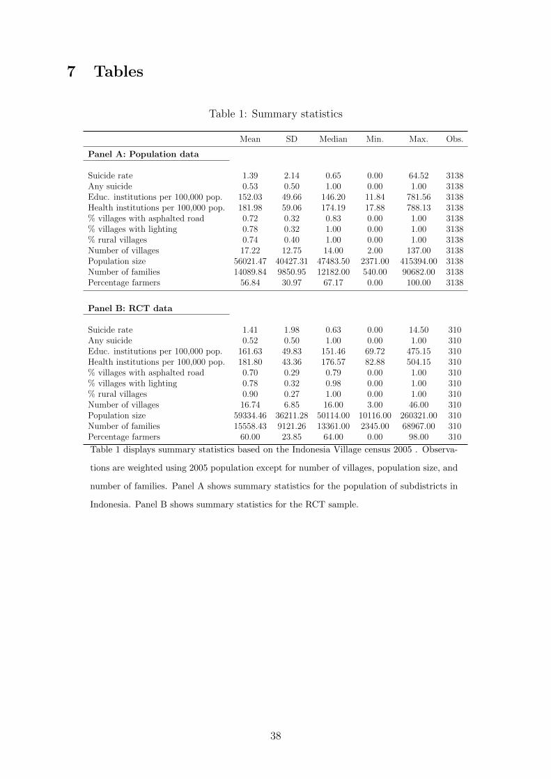
7 Tables

Table 1: Summary statistics

Mean SD Median Min. Max. Obs.

Panel A: Population data

Suicide rate 1.39 2.14 0.65 0.00 64.52 3138Any suicide 0.53 0.50 1.00 0.00 1.00 3138Educ. institutions per 100,000 pop. 152.03 49.66 146.20 11.84 781.56 3138Health institutions per 100,000 pop. 181.98 59.06 174.19 17.88 788.13 3138% villages with asphalted road 0.72 0.32 0.83 0.00 1.00 3138% villages with lighting 0.78 0.32 1.00 0.00 1.00 3138% rural villages 0.74 0.40 1.00 0.00 1.00 3138Number of villages 17.22 12.75 14.00 2.00 137.00 3138Population size 56021.47 40427.31 47483.50 2371.00 415394.00 3138Number of families 14089.84 9850.95 12182.00 540.00 90682.00 3138Percentage farmers 56.84 30.97 67.17 0.00 100.00 3138

Panel B: RCT data

Suicide rate 1.41 1.98 0.63 0.00 14.50 310Any suicide 0.52 0.50 1.00 0.00 1.00 310Educ. institutions per 100,000 pop. 161.63 49.83 151.46 69.72 475.15 310Health institutions per 100,000 pop. 181.80 43.36 176.57 82.88 504.15 310% villages with asphalted road 0.70 0.29 0.79 0.00 1.00 310% villages with lighting 0.78 0.32 0.98 0.00 1.00 310% rural villages 0.90 0.27 1.00 0.00 1.00 310Number of villages 16.74 6.85 16.00 3.00 46.00 310Population size 59334.46 36211.28 50114.00 10116.00 260321.00 310Number of families 15558.43 9121.26 13361.00 2345.00 68967.00 310Percentage farmers 60.00 23.85 64.00 0.00 98.00 310

Table 1 displays summary statistics based on the Indonesia Village census 2005 . Observa-

tions are weighted using 2005 population except for number of villages, population size, and

number of families. Panel A shows summary statistics for the population of subdistricts in

Indonesia. Panel B shows summary statistics for the RCT sample.

38

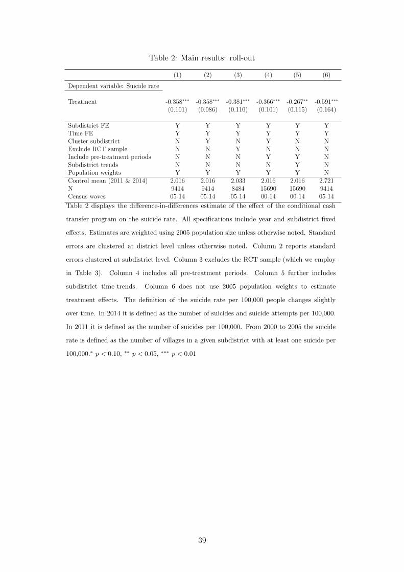
Table 2: Main results: roll-out

(1) (2) (3) (4) (5) (6)

Dependent variable: Suicide rate

Treatment -0.358∗∗∗ -0.358∗∗∗ -0.381∗∗∗ -0.366∗∗∗ -0.267∗∗ -0.591∗∗∗

(0.101) (0.086) (0.110) (0.101) (0.115) (0.164)

Subdistrict FE Y Y Y Y Y YTime FE Y Y Y Y Y YCluster subdistrict N Y N Y N NExclude RCT sample N N Y N N NInclude pre-treatment periods N N N Y Y NSubdistrict trends N N N N Y NPopulation weights Y Y Y Y Y NControl mean (2011 & 2014) 2.016 2.016 2.033 2.016 2.016 2.721N 9414 9414 8484 15690 15690 9414Census waves 05-14 05-14 05-14 00-14 00-14 05-14

Table 2 displays the difference-in-differences estimate of the effect of the conditional cash

transfer program on the suicide rate. All specifications include year and subdistrict fixed

effects. Estimates are weighted using 2005 population size unless otherwise noted. Standard

errors are clustered at district level unless otherwise noted. Column 2 reports standard

errors clustered at subdistrict level. Column 3 excludes the RCT sample (which we employ

in Table 3). Column 4 includes all pre-treatment periods. Column 5 further includes

subdistrict time-trends. Column 6 does not use 2005 population weights to estimate

treatment effects. The definition of the suicide rate per 100,000 people changes slightly

over time. In 2014 it is defined as the number of suicides and suicide attempts per 100,000.

In 2011 it is defined as the number of suicides per 100,000. From 2000 to 2005 the suicide

rate is defined as the number of villages in a given subdistrict with at least one suicide per

100,000.∗ p < 0.10, ∗∗ p < 0.05, ∗∗∗ p < 0.01

39

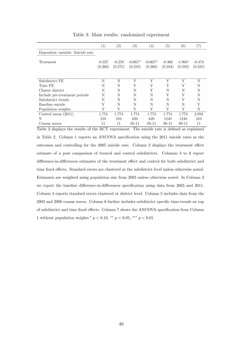
Table 3: Main results: randomized experiment

(1) (2) (3) (4) (5) (6) (7)

Dependent variable: Suicide rate

Treatment -0.337 -0.258 -0.665∗∗ -0.665∗∗ -0.466 -1.064∗ -0.474(0.266) (0.275) (0.318) (0.266) (0.334) (0.593) (0.325)

Subdistrict FE N N Y Y Y Y NTime FE N N Y Y Y Y NCluster district N N N Y N N NInclude pre-treatment periods N N N N Y Y NSubdistrict trends N N N N N Y NBaseline suicide Y N N N N N YPopulation weights Y Y Y Y Y Y NControl mean (2011) 1.774 1.774 1.774 1.774 1.774 1.774 2.058N 310 310 620 620 1240 1240 310Census waves 11 11 05-11 05-11 00-11 00-11 11

Table 3 displays the results of the RCT experiment. The suicide rate is defined as explained

in Table 2. Column 1 reports an ANCOVA specification using the 2011 suicide rates as the

outcomes and controlling for the 2005 suicide rate. Column 2 displays the treatment effect

estimate of a post comparison of treated and control subdistricts. Columns 3 to 6 report

difference-in-differences estimates of the treatment effect and control for both subdistrict and

time fixed effects. Standard errors are clustered at the subdistrict level unless otherwise noted.

Estimates are weighted using population size from 2005 unless otherwise noted. In Column 3

we report the baseline difference-in-differences specification using data from 2005 and 2011.

Column 4 reports standard errors clustered at district level. Column 5 includes data from the

2003 and 2000 census waves. Column 6 further includes subdistrict specific time-trends on top

of subdistrict and time fixed effects. Column 7 shows the ANCOVA specification from Column

1 without population weights.∗ p < 0.10, ∗∗ p < 0.05, ∗∗∗ p < 0.01

40

Table 4: Interactions between agricultural productivity shocks and the cash transfers

(1) (2) (3) (4) (5) (6)

Dependent variable: Suicide rate

Rain (z-scored) -0.082∗ -0.112∗∗ -0.081∗ -0.106∗∗ -0.094∗ -0.129∗∗

(0.045) (0.050) (0.044) (0.048) (0.049) (0.054)[0.039] [0.043] [0.038] [0.042] [0.039] [0.046]

Treat -0.216∗∗ -0.255∗∗ -0.193(0.109) (0.101) (0.117)[0.122] [0.115] [0.130]

Rain (z-scored)× Treat 0.118∗ 0.096 0.133∗

(0.072) (0.068) (0.079)[0.070] [0.068] [0.077]

Subdistrict FE Y Y Y Y Y YTime FE Y Y Y Y Y YSubdistrict trends N N Y Y N NInclude lagged rainfall N N N N Y Y

N 15690 15690 15690 15690 15690 15690Census waves 00-14 00-14 00-14 00-14 00-14 00-14

Table 4 displays the impact of rainfall on the suicide rate. The suicide rate is defined as explained

in Table 2. Odd columns report the impact of standardized rainfall on suicides. Even columns

include the treatment variable from the conditional cash transfer roll-out and the interaction with

rainfall. All specifications include subdistrict and year fixed effects. Columns 3 and 4 control

for subdistrict time-trends. Columns 5 and 6 include the first, second and third lag of rainfall.

Parentheses report Conley (1999) standard errors, allowing for arbitrary time correlation and

two-dimensional spatial correlation within a 100 kilometre radius of the subdistrict centroid (used

for stars). Standard errors clustered at the district level are in square brackets. ∗ p < 0.10, ∗∗

p < 0.05, ∗∗∗ p < 0.01

41

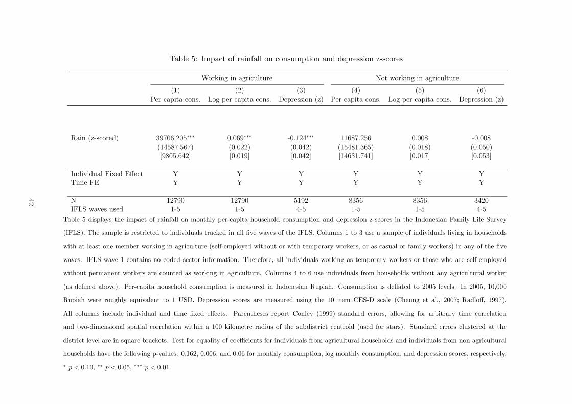
Table 5: Impact of rainfall on consumption and depression z-scores

Working in agriculture Not working in agriculture

(1) (2) (3) (4) (5) (6)Per capita cons. Log per capita cons. Depression (z) Per capita cons. Log per capita cons. Depression (z)

Rain (z-scored) 39706.205∗∗∗ 0.069∗∗∗ -0.124∗∗∗ 11687.256 0.008 -0.008(14587.567) (0.022) (0.042) (15481.365) (0.018) (0.050)[9805.642] [0.019] [0.042] [14631.741] [0.017] [0.053]

Individual Fixed Effect Y Y Y Y Y YTime FE Y Y Y Y Y Y

N 12790 12790 5192 8356 8356 3420IFLS waves used 1-5 1-5 4-5 1-5 1-5 4-5

Table 5 displays the impact of rainfall on monthly per-capita household consumption and depression z-scores in the Indonesian Family Life Survey

(IFLS). The sample is restricted to individuals tracked in all five waves of the IFLS. Columns 1 to 3 use a sample of individuals living in households

with at least one member working in agriculture (self-employed without or with temporary workers, or as casual or family workers) in any of the five

waves. IFLS wave 1 contains no coded sector information. Therefore, all individuals working as temporary workers or those who are self-employed

without permanent workers are counted as working in agriculture. Columns 4 to 6 use individuals from households without any agricultural worker

(as defined above). Per-capita household consumption is measured in Indonesian Rupiah. Consumption is deflated to 2005 levels. In 2005, 10,000

Rupiah were roughly equivalent to 1 USD. Depression scores are measured using the 10 item CES-D scale (Cheung et al., 2007; Radloff, 1997).

All columns include individual and time fixed effects. Parentheses report Conley (1999) standard errors, allowing for arbitrary time correlation

and two-dimensional spatial correlation within a 100 kilometre radius of the subdistrict centroid (used for stars). Standard errors clustered at the

district level are in square brackets. Test for equality of coefficients for individuals from agricultural households and individuals from non-agricultural

households have the following p-values: 0.162, 0.006, and 0.06 for monthly consumption, log monthly consumption, and depression scores, respectively.

∗ p < 0.10, ∗∗ p < 0.05, ∗∗∗ p < 0.01

42

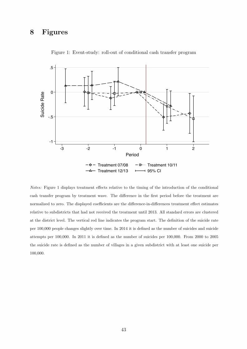
8 Figures

Figure 1: Event-study: roll-out of conditional cash transfer program

-1

-.5

0

.5

Suic

ide

Rat

e

-3 -2 -1 0 1 2Period

Treatment 07/08 Treatment 10/11Treatment 12/13 95% CI

Notes: Figure 1 displays treatment effects relative to the timing of the introduction of the conditional

cash transfer program by treatment wave. The difference in the first period before the treatment are

normalized to zero. The displayed coefficients are the difference-in-differences treatment effect estimates

relative to subdistricts that had not received the treatment until 2013. All standard errors are clustered

at the district level. The vertical red line indicates the program start. The definition of the suicide rate

per 100,000 people changes slightly over time. In 2014 it is defined as the number of suicides and suicide

attempts per 100,000. In 2011 it is defined as the number of suicides per 100,000. From 2000 to 2005

the suicide rate is defined as the number of villages in a given subdistrict with at least one suicide per

100,000.

43

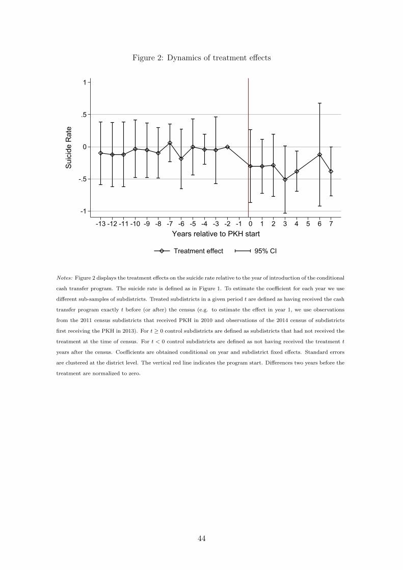
Figure 2: Dynamics of treatment effects

-1

-.5

0

.5

1

Suic

ide

Rat

e

-13 -12 -11 -10 -9 -8 -7 -6 -5 -4 -3 -2 -1 0 1 2 3 4 5 6 7Years relative to PKH start

Treatment effect 95% CI

Notes: Figure 2 displays the treatment effects on the suicide rate relative to the year of introduction of the conditional

cash transfer program. The suicide rate is defined as in Figure 1. To estimate the coefficient for each year we use

different sub-samples of subdistricts. Treated subdistricts in a given period t are defined as having received the cash

transfer program exactly t before (or after) the census (e.g. to estimate the effect in year 1, we use observations

from the 2011 census subdistricts that received PKH in 2010 and observations of the 2014 census of subdistricts

first receiving the PKH in 2013). For t ≥ 0 control subdistricts are defined as subdistricts that had not received the

treatment at the time of census. For t < 0 control subdistricts are defined as not having received the treatment t

years after the census. Coefficients are obtained conditional on year and subdistrict fixed effects. Standard errors

are clustered at the district level. The vertical red line indicates the program start. Differences two years before the

treatment are normalized to zero.

44

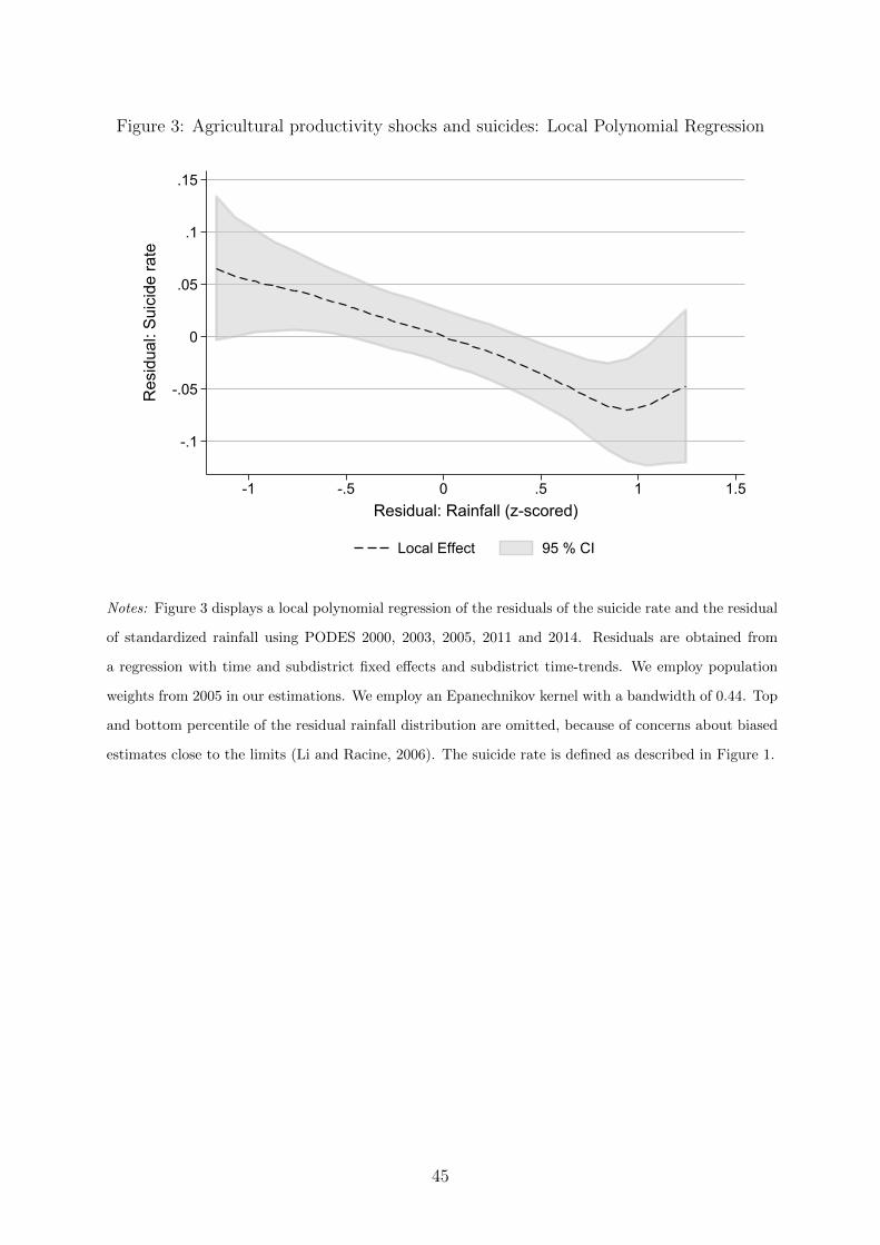
Figure 3: Agricultural productivity shocks and suicides: Local Polynomial Regression

-.1

-.05

0

.05

.1

.15

Res

idua

l: Su

icid

e ra

te

-1 -.5 0 .5 1 1.5Residual: Rainfall (z-scored)

Local Effect 95 % CI

Notes: Figure 3 displays a local polynomial regression of the residuals of the suicide rate and the residual

of standardized rainfall using PODES 2000, 2003, 2005, 2011 and 2014. Residuals are obtained from

a regression with time and subdistrict fixed effects and subdistrict time-trends. We employ population

weights from 2005 in our estimations. We employ an Epanechnikov kernel with a bandwidth of 0.44. Top

and bottom percentile of the residual rainfall distribution are omitted, because of concerns about biased

estimates close to the limits (Li and Racine, 2006). The suicide rate is defined as described in Figure 1.

45

Online Appendix: Income Shocks and Suicides:Causal Evidence From Indonesia

Cornelius Christian, Lukas Hensel, and Christopher Roth

Summary of the Online appendix

The Appendix starts with detailing the calculations used to obtain the direct effect sizes

discussed in Section 5 of the paper.

In Section A.2 we present descriptive statistics. Table A.1 shows correlates of suicide

rates. Table A.2 shows evidence in favor of the integrity of the randomization. Section A.3

examines the sensitivity of our results from the difference-in-differences strategy. Table

A.3 provides further checks on the assumption that the timing of roll-out of the program

was quasi-random. Tables A.4 and A.5 examine robustness of the roll-out results to using

different definitions of the outcome variables. Table A.6 examine sensitivity of our results

to dropping partially treated subdistricts. Table A.7 shows the main roll-out results

without using population weights. Table A.8 shows the results using 2006 subdistrict

definitions. Table A.9 shows further robustness checks.

Section A.4 examines the sensitivity of the results from the randomized cash trans-

fer program. Tables A.10 and A.11 examine robustness of the RCT results to using

different definitions of the outcome variables. Table A.12 examines sensitivity of our

results to dropping partially treated subdistricts. Table A.13 shows the RCT results

without employing population weights. Table A.14 shows the results using 2006 subdis-

trict definitions. Finally, Table A.15 shows further robustness checks for the RCT results.

Section A.5 presents further analysis of the dynamics of treatment effects. Table A.16

present the results on “dynamic treatment effects” which using population weights. Table

A.17 present the results on “dynamic treatment effects” which does not apply population

weights. Table A.18 examines whether treatment effects vary with treatment intensity.

Section A.6 provides further robustness checks for the rainfall analysis. Table A.19

1

examines whether rainfall and suicide rates are symmetrically related. Table A.20 presents

the main specifications without using population weights. Table A.21 examines whether

the interaction of rainfall and conditional cash transfers are non-linearly related. Table

A.22 shows the main specification with rainfall detrended at the subdistrict level using

population weights. Table A.23 shows the main specification with rainfall detrended at

the subdistrict level without using population weights.

Section A.7 presents micro-evidence using the Indonesian Family Life Survey. Table

A.24 analyzes heterogeneous effect of rainfall shocks on depression symptoms by gender,

age and baseline expenditures. Table A.25 examines whether PKH recipients have higher

depression scores before the receipt of the cash transfer program.

Section A.8 sheds further light on mechanisms. Table A.26 examines whether our

results are mediated by changes in crime rates, the quality of local institutions or social

capital. Table A.27 describes heterogeneous responses to the treatment.

Section B presents additional figures. Figure A.1 displays the evolution of mean suicide

rates over time for different treatment groups. Figure A.2 displays mean suicide rates

over time by treatment wave without applying population weights. Figure A.3 shows

the event-study analysis without applying population weights. Figure A.4 presents an

event-study analysis for our RCT sample with effects normalized relative to 2005. Figure

A.4 presents an event-study analysis for our RCT sample with effects normalized relative

to 2000. Figure A.4 presents an event-study analysis for our RCT sample. Figure A.6

displays mean suicide rates (based on a Poisson extrapolation) over time by treatment

wave. Finally, Figure A.7 showcases the event-study graph using the Poisson extrapolated

suicide rates.

2

A Online Appendix

A.1 Effect Size Calculations

This section explains how we calculate the implied direct effect on cash transfer recipients

and farmers. This section is not meant to provide unambiguous estimates of direct effects,

but rather to provide a back of the envelope calculation based on several simplifying

assumptions. We conduct this analysis in the following steps for the cash transfer program

and agricultural productivity shocks.

1. Calculate the economic gradient of suicide rates.

2. Calculate the implied direct treatment effect on treated individuals.

3. Account for potential spillover effects of changing suicide rates.

A.1.1 The Cash Transfer Program

First, we calculate the economic gradient of the suicide rate with respect to being classified

as poor. We use this specification as a proxy for households eligible to receive PKH.1

Column 1 of Table A.1 suggests that a 10% higher share of the eligible household is, on

average, associated with a 0.142 higher suicide rate 2005 before the program was rolled

out. Assuming that this linear relationship between the fraction of poor individuals

and the suicide rate holds we can use the constant as the suicide rate for non-eligible

individuals (snon-elig = 1.15 ). The relationship between the share of eligible individuals

(xelig = 0.1) and the suicide rate is:

1.15 + 1.42 · xelig = (1− xelig) · 1.15 + xelig · selig

1 We abstract from the fact that 15% of the population is classified as poor and assuming that 10%

of the population is poor and that only these 10% are eligible for treatment. If anything this would

make us underestimate the economic gradient between PKH recipient and non-recipients.

3

From this we obtain the implied suicide rate for poor individuals selig = 2.57. Thus,

we conclude that eligible individuals are 2.24 times more likely to commit suicides than

non-eligible individuals.

Second, we calculate the implied direct effect on eligible individuals assume that this

ratio of suicide rates for eligible and non-eligible individuals relationship remains the same

for 2011 and 2014 for non-treated subdistricts. As a first step, we calculate the implied

suicide rates for eligible and non-eligible individuals in 2011 and 2014. The control mean

(scontrol = 2.02) is equal to a weighted average of eligible and non-eligible individuals:

scontrol = 2.02 = 0.9 · snon-elig + 0.1 · 2.24 · snon-elig︸ ︷︷ ︸selig

(6)

From this we obtain snon-elig = 1.80 and selig = 4.03. Next, we use the calculated suicide

rate in treated subdistricts streat = 2.02 − 0.36 = 1.66 to calculate the implied direct

treatment effect on eligible individuals. Assuming no spillovers on untreated individuals

we obtain:

0.9 · 1.8 + 0.1 · (4.03 + ∆selig) = 1.66 (7)

.

This yields a direct treatment effect on PKH recipients as ∆selig = −3.6 or a reduction

of about 89% of the implied control suicide rate for eligible individuals.

These numbers imply that the suicide rate of eligible individuals receiving the cash

transfer would be reduced to levels below the suicide rate of non-eligible households.

Therefore, we conduct a further calculation allowing for the cash transfer program to

have positive spillovers on non-eligible individuals, in line with evidence on cash transfers

and suicides (Angelucci and De Giorgi, 2009; Hedstrom et al., 2008). Our benchmark

specification calibrates the strength of within subdistrict spill-overs such that the ex-post

suicide rates of eligible and non-eligible individuals in treated subdistricts is equalized.

We model the total treatment effect as consisting of a multiplier effect and a direct

treatment effect. This requires an assumption about the functional form of the multiplier.

4

We assume that the suicide rate of non-PKH recipients in treated subdistricts is a function

of the direct treatment effect times a multiplier µ. The suicide rate in treated subdistricts

can then be written as:

streat = 0.9 · (scontr,non-elig + µ(streat,elig − scontr,elig)︸ ︷︷ ︸Spill-overs

) + 0.1 · streat,elig (8)

From this we can obtain the implied direct treatment effect on PKH recipients as:

∆selig = streat,elig − scontr,elig =streat − 0.9 · scontr, non-elig − 0.1 · scontr,elig

0.9 · µ+ 0.1(9)

Equation 9 confirms the intuition that the implied direct effect on poor individuals

decreases with size of the multiplier µ. Setting ex-post suicide rates for poor and non-

eligible individuals equal at the mean suicide rate in treated subdistricts of 1.66 suicides

per 100,000, we obtain a multiplier of µ = 0.049 and an implied direct effect on PKH

recipients of 2.36 per 100,000 or 58.7% of the implied control group mean.

Effect on number of suicides Our preferred estimate for the number of suicides is

Column 11 of Table A.5 which shows an average treatment effect of 0.2 suicides. In total,

there we observe 5324 subdistrict-years for treated subdistricts over time. Assuming

constant treatment effects over time, we calculate that the PKH program prevented 1065

suicides.

A.1.2 Rainfall

To calculate the effect size of agricultural productivity shocks, we conduct a similar

calculation.

First, we obtain the economic gradient of the suicide rate with the share of farmers

using the results from Column 2 of Table A.1. We observe that in 2005 an increase in

the share of farmer by 10% is associated with an increase in the suicide rate of 1.19. The

5

population weighted average share of farmers in 2005 is xfarm = 0.56.2

We again use the constant as the suicide rate for non-farmers (snon-farm = 0.72 ). The

relationship between the share of farmers xfarm and the suicide rate is:

0.72 + 1.19 · xfarm = (1− xfarm) · 0.71 + xfarm · sfarm

From this we obtain the implied suicide rate for farmers sfarm = 1.91. Thus, farmers

are 2.67 time more likely to commit suicides than non-farmers households. The calcula-

tions for the effect of rainfall are complicated by the fact that there is no clear control

group. Therefore, we use the population weighted mean suicide rate across all years (1.39

suicides per 100,000). Assuming no spill-over effects, we then calculate the implied suicide

rates for farmers and non-farmers using the following equation:

s = 1.39 = 0.44 · scontr,non-farm + 0.56 · 2.67 · scontr, non-farm︸ ︷︷ ︸=scontr, farm

We obtain mean suicide rates of scontr, farm = 1.91 for farmers and scontr, non-farm = 0.72

for non-farmers

Based on these implied means we can then calculate the implied direct effect size as-

suming no spill-overs. The average effect of a one-standard deviation in rainfall according

to our preferred specification is −0.08. We obtain streat = 1.31 by subtracting a one stan-

dard deviation treatment effect (0.08) from the population weighted mean suicide rate

across all years (1.39). We then use an analogue equation to the cash transfer calculations

to compute the implied direct effect:

streat = 1.31 = 0.44 · scontr,non-farm + 0.56 · (scontr, farm + ∆sfarm)

With these assumptions, we obtain an implied direct effect size as ∆sfarm = −0.14

which is equivalent to 7.4 percent of the implied long-term mean for farmers. Allowing

2 We use the 2005 share to make the calculation comparable to the cash transfer calculations.

6

for spillover with a multiplier in line with the cash transfer (0.049), the implied direct

treatment effect decreases to −0.047 suicides per 100,000 or 2.5 percent of the implied

long-term mean for farmers.

A.1.3 Calculating per-dollar impacts for implied direct effects

This section outlines how we calculate comparable monetary values for implied direct

effect of the cash transfer and agricultural productivity shocks. For this exercise, we

need to assume that the impact is linear in dollar amounts. For the cash transfer, we

estimate that 22.45 USD lower the suicide rate by 3.6 suicides per 100,000 or 89 percent,

so that 10 USD would lower the suicide rate by 1.61 suicides per 100,000 or 39.64 percent.

For agricultural productivity shocks, we estimate that a yearly per-capita consumption

increase by 21.6 USD reduces the suicide rate by 0.14 suicides per 100,000 or 7.4 percent.

This implies that 10 USD would reduce the suicide rate by 0.06 suicides per 100,000 or

3.34 percent.

7

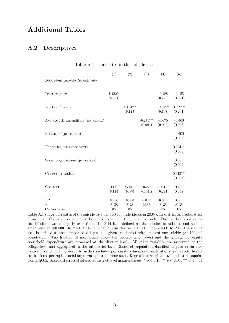
Additional Tables

A.2 Descriptives

Table A.1: Correlates of the suicide rate

(1) (2) (3) (4) (5)

Dependent variable: Suicide rate

Fraction poor 1.422∗∗ -0.488 -0.155(0.591) (0.721) (0.684)

Fraction farmers 1.194∗∗∗ 1.109∗∗∗ 0.692∗∗∗

(0.129) (0.168) (0.204)

Average HH expenditure (per capita) -0.273∗∗∗ -0.075 -0.063(0.051) (0.067) (0.066)

Education (per capita) -0.000(0.001)

Health facilities (per capita) 0.004∗∗∗

(0.001)

Social organisations (per capita) 0.000(0.000)

Crime (per capita) 0.013∗∗∗

(0.003)

Constant 1.147∗∗∗ 0.715∗∗∗ 2.035∗∗∗ 1.024∗∗∗ 0.120(0.114) (0.070) (0.144) (0.294) (0.348)

R2 0.006 0.030 0.017 0.030 0.066N 3138 3138 3138 3138 3138Census wave 05 05 05 05 05

Table A.1 shows correlates of the suicide rate per 100,000 individuals in 2005 with district and subdistrictcovariates. Our main outcome is the suicide rate per 100,000 individuals. Due to data constraintsits definition varies slightly over time. In 2014 it is defined as the number of suicides and suicideattempts per 100,000. In 2011 it the number of suicides per 100,000. From 2000 to 2005 the suiciderate is defined as the number of villages in a given subdistrict with at least one suicide per 100,000population. The fraction of individuals below the poverty line (poor) and the average per-capitahousehold expenditure are measured at the district level. All other variables are measured at thevillage level and aggregated to the subdistrict level. Share of population classified as poor or farmersranges from 0 to 1. Column 5 further includes per capita educational institutions, per capita healthinstitutions, per capita social organizations, and crime rates. Regressions weighted by subdistrict popula-tion in 2005. Standard errors clustered at district level in parentheses. ∗ p < 0.10, ∗∗ p < 0.05, ∗∗∗ p < 0.01

8

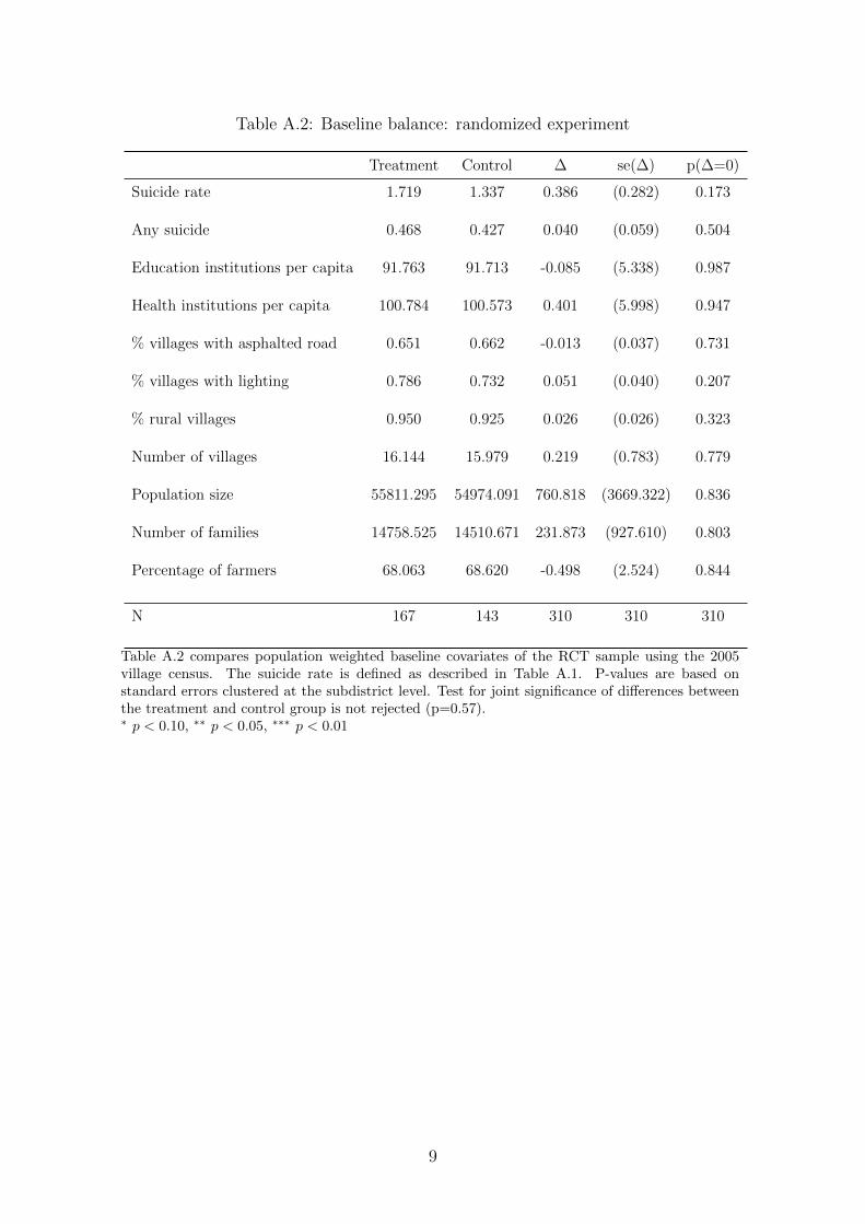
Table A.2: Baseline balance: randomized experiment

Treatment Control ∆ se(∆) p(∆=0)

Suicide rate 1.719 1.337 0.386 (0.282) 0.173

Any suicide 0.468 0.427 0.040 (0.059) 0.504

Education institutions per capita 91.763 91.713 -0.085 (5.338) 0.987

Health institutions per capita 100.784 100.573 0.401 (5.998) 0.947

% villages with asphalted road 0.651 0.662 -0.013 (0.037) 0.731

% villages with lighting 0.786 0.732 0.051 (0.040) 0.207

% rural villages 0.950 0.925 0.026 (0.026) 0.323

Number of villages 16.144 15.979 0.219 (0.783) 0.779

Population size 55811.295 54974.091 760.818 (3669.322) 0.836

Number of families 14758.525 14510.671 231.873 (927.610) 0.803

Percentage of farmers 68.063 68.620 -0.498 (2.524) 0.844

N 167 143 310 310 310

Table A.2 compares population weighted baseline covariates of the RCT sample using the 2005village census. The suicide rate is defined as described in Table A.1. P-values are based onstandard errors clustered at the subdistrict level. Test for joint significance of differences betweenthe treatment and control group is not rejected (p=0.57).∗ p < 0.10, ∗∗ p < 0.05, ∗∗∗ p < 0.01

9

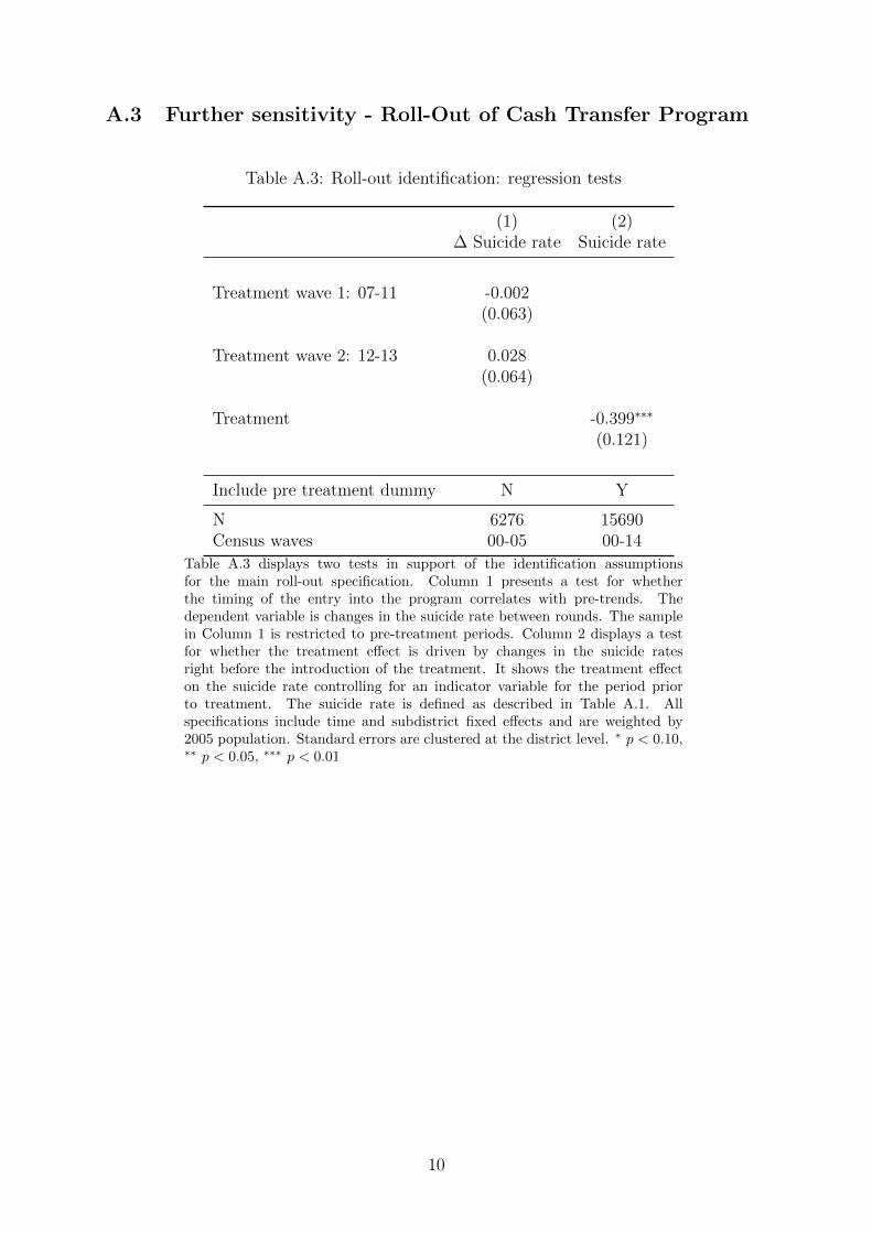
A.3 Further sensitivity - Roll-Out of Cash Transfer Program

Table A.3: Roll-out identification: regression tests

(1) (2)∆ Suicide rate Suicide rate

Treatment wave 1: 07-11 -0.002(0.063)

Treatment wave 2: 12-13 0.028(0.064)

Treatment -0.399∗∗∗

(0.121)

Include pre treatment dummy N Y

N 6276 15690Census waves 00-05 00-14

Table A.3 displays two tests in support of the identification assumptionsfor the main roll-out specification. Column 1 presents a test for whetherthe timing of the entry into the program correlates with pre-trends. Thedependent variable is changes in the suicide rate between rounds. The samplein Column 1 is restricted to pre-treatment periods. Column 2 displays a testfor whether the treatment effect is driven by changes in the suicide ratesright before the introduction of the treatment. It shows the treatment effecton the suicide rate controlling for an indicator variable for the period priorto treatment. The suicide rate is defined as described in Table A.1. Allspecifications include time and subdistrict fixed effects and are weighted by2005 population. Standard errors are clustered at the district level. ∗ p < 0.10,∗∗ p < 0.05, ∗∗∗ p < 0.01

10

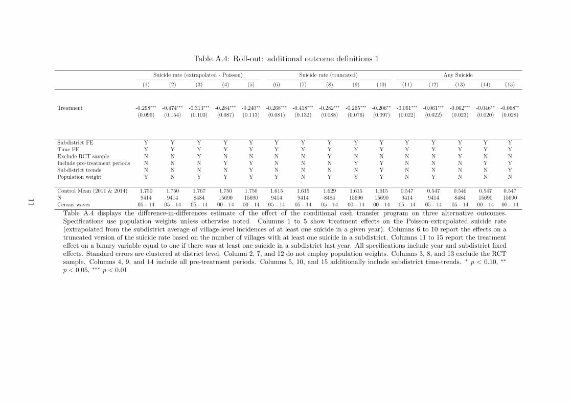
Table A.4: Roll-out: additional outcome definitions 1

Suicide rate (extrapolated - Poisson) Suicide rate (truncated) Any Suicide

(1) (2) (3) (4) (5) (6) (7) (8) (9) (10) (11) (12) (13) (14) (15)

Treatment -0.298∗∗∗ -0.474∗∗∗ -0.313∗∗∗ -0.284∗∗∗ -0.240∗∗ -0.268∗∗∗ -0.418∗∗∗ -0.282∗∗∗ -0.265∗∗∗ -0.206∗∗ -0.061∗∗∗ -0.061∗∗∗ -0.062∗∗∗ -0.046∗∗ -0.068∗∗

(0.096) (0.154) (0.103) (0.087) (0.113) (0.081) (0.132) (0.088) (0.076) (0.097) (0.022) (0.022) (0.023) (0.020) (0.028)

Subdistrict FE Y Y Y Y Y Y Y Y Y Y Y Y Y Y YTime FE Y Y Y Y Y Y Y Y Y Y Y Y Y Y YExclude RCT sample N N Y N N N N Y N N N N Y N NInclude pre-treatment periods N N N Y Y N N N Y Y N N N Y YSubdistrict trends N N N N Y N N N N Y N N N N YPopulation weight Y N Y Y Y Y N Y Y Y N Y N N N

Control Mean (2011 & 2014) 1.750 1.750 1.767 1.750 1.750 1.615 1.615 1.629 1.615 1.615 0.547 0.547 0.546 0.547 0.547N 9414 9414 8484 15690 15690 9414 9414 8484 15690 15690 9414 9414 8484 15690 15690Census waves 05 - 14 05 - 14 05 - 14 00 - 14 00 - 14 05 - 14 05 - 14 05 - 14 00 - 14 00 - 14 05 - 14 05 - 14 05 - 14 00 - 14 00 - 14

Table A.4 displays the difference-in-differences estimate of the effect of the conditional cash transfer program on three alternative outcomes.Specifications use population weights unless otherwise noted. Columns 1 to 5 show treatment effects on the Poisson-extrapolated suicide rate(extrapolated from the subdistrict average of village-level incidences of at least one suicide in a given year). Columns 6 to 10 report the effects on atruncated version of the suicide rate based on the number of villages with at least one suicide in a subdistrict. Columns 11 to 15 report the treatmenteffect on a binary variable equal to one if there was at least one suicide in a subdistrict last year. All specifications include year and subdistrict fixedeffects. Standard errors are clustered at district level. Column 2, 7, and 12 do not employ population weights. Columns 3, 8, and 13 exclude the RCTsample. Columns 4, 9, and 14 include all pre-treatment periods. Columns 5, 10, and 15 additionally include subdistrict time-trends. ∗ p < 0.10, ∗∗

p < 0.05, ∗∗∗ p < 0.01

11

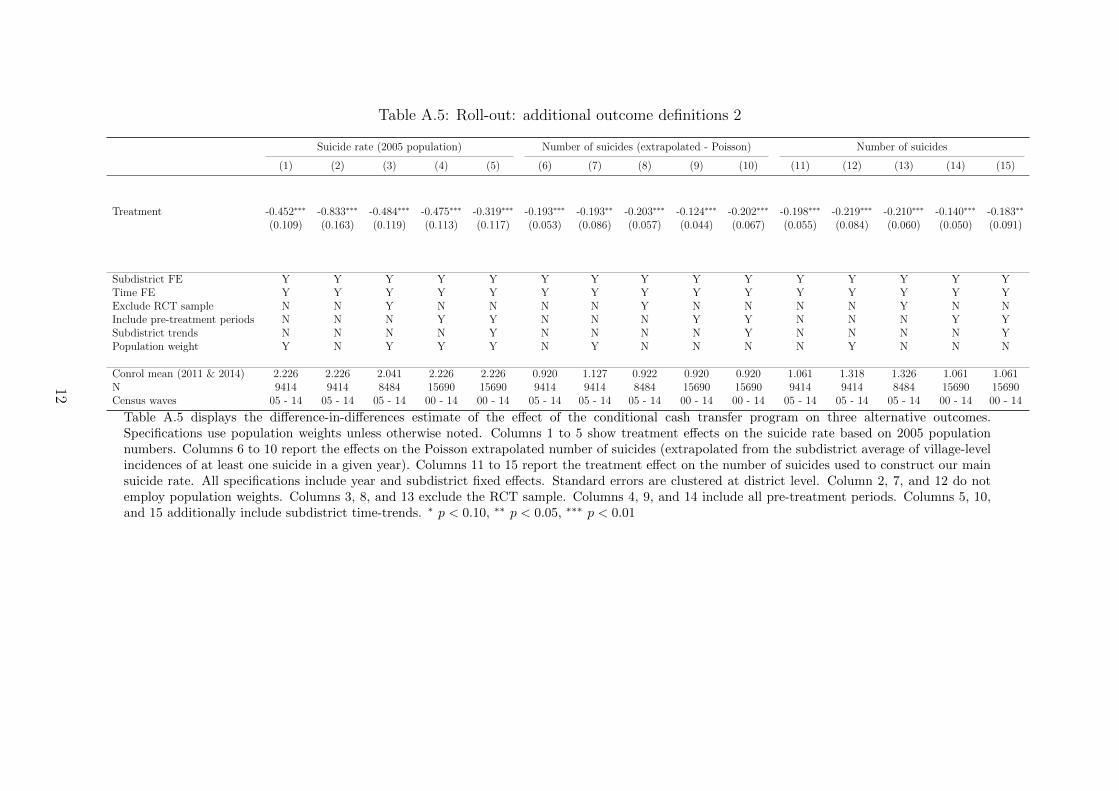
Table A.5: Roll-out: additional outcome definitions 2

Suicide rate (2005 population) Number of suicides (extrapolated - Poisson) Number of suicides

(1) (2) (3) (4) (5) (6) (7) (8) (9) (10) (11) (12) (13) (14) (15)

Treatment -0.452∗∗∗ -0.833∗∗∗ -0.484∗∗∗ -0.475∗∗∗ -0.319∗∗∗ -0.193∗∗∗ -0.193∗∗ -0.203∗∗∗ -0.124∗∗∗ -0.202∗∗∗ -0.198∗∗∗ -0.219∗∗∗ -0.210∗∗∗ -0.140∗∗∗ -0.183∗∗

(0.109) (0.163) (0.119) (0.113) (0.117) (0.053) (0.086) (0.057) (0.044) (0.067) (0.055) (0.084) (0.060) (0.050) (0.091)

Subdistrict FE Y Y Y Y Y Y Y Y Y Y Y Y Y Y YTime FE Y Y Y Y Y Y Y Y Y Y Y Y Y Y YExclude RCT sample N N Y N N N N Y N N N N Y N NInclude pre-treatment periods N N N Y Y N N N Y Y N N N Y YSubdistrict trends N N N N Y N N N N Y N N N N YPopulation weight Y N Y Y Y N Y N N N N Y N N N

Conrol mean (2011 & 2014) 2.226 2.226 2.041 2.226 2.226 0.920 1.127 0.922 0.920 0.920 1.061 1.318 1.326 1.061 1.061N 9414 9414 8484 15690 15690 9414 9414 8484 15690 15690 9414 9414 8484 15690 15690Census waves 05 - 14 05 - 14 05 - 14 00 - 14 00 - 14 05 - 14 05 - 14 05 - 14 00 - 14 00 - 14 05 - 14 05 - 14 05 - 14 00 - 14 00 - 14

Table A.5 displays the difference-in-differences estimate of the effect of the conditional cash transfer program on three alternative outcomes.Specifications use population weights unless otherwise noted. Columns 1 to 5 show treatment effects on the suicide rate based on 2005 populationnumbers. Columns 6 to 10 report the effects on the Poisson extrapolated number of suicides (extrapolated from the subdistrict average of village-levelincidences of at least one suicide in a given year). Columns 11 to 15 report the treatment effect on the number of suicides used to construct our mainsuicide rate. All specifications include year and subdistrict fixed effects. Standard errors are clustered at district level. Column 2, 7, and 12 do notemploy population weights. Columns 3, 8, and 13 exclude the RCT sample. Columns 4, 9, and 14 include all pre-treatment periods. Columns 5, 10,and 15 additionally include subdistrict time-trends. ∗ p < 0.10, ∗∗ p < 0.05, ∗∗∗ p < 0.01

12

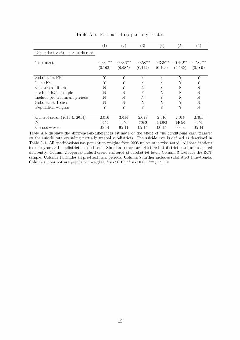
Table A.6: Roll-out: drop partially treated

(1) (2) (3) (4) (5) (6)

Dependent variable: Suicide rate

Treatment -0.336∗∗∗ -0.336∗∗∗ -0.358∗∗∗ -0.339∗∗∗ -0.442∗∗ -0.582∗∗∗

(0.103) (0.087) (0.112) (0.103) (0.180) (0.169)

Subdistrict FE Y Y Y Y Y YTime FE Y Y Y Y Y YCluster subdistrict N Y N Y N NExclude RCT sample N N Y N N NInclude pre-treatment periods N N N Y N NSubdistrict Trends N N N N Y NPopulation weights Y Y Y Y Y N

Control mean (2011 & 2014) 2.016 2.016 2.033 2.016 2.016 2.391N 8454 8454 7686 14090 14090 8454Census waves 05-14 05-14 05-14 00-14 00-14 05-14

Table A.6 displays the difference-in-differences estimate of the effect of the conditional cash transferon the suicide rate excluding partially treated subdistricts. The suicide rate is defined as described inTable A.1. All specifications use population weights from 2005 unless otherwise noted. All specificationsinclude year and subdistrict fixed effects. Standard errors are clustered at district level unless noteddifferently. Column 2 report standard errors clustered at subdistrict level. Column 3 excludes the RCTsample. Column 4 includes all pre-treatment periods. Column 5 further includes subdistrict time-trends.Column 6 does not use population weights. ∗ p < 0.10, ∗∗ p < 0.05, ∗∗∗ p < 0.01

13

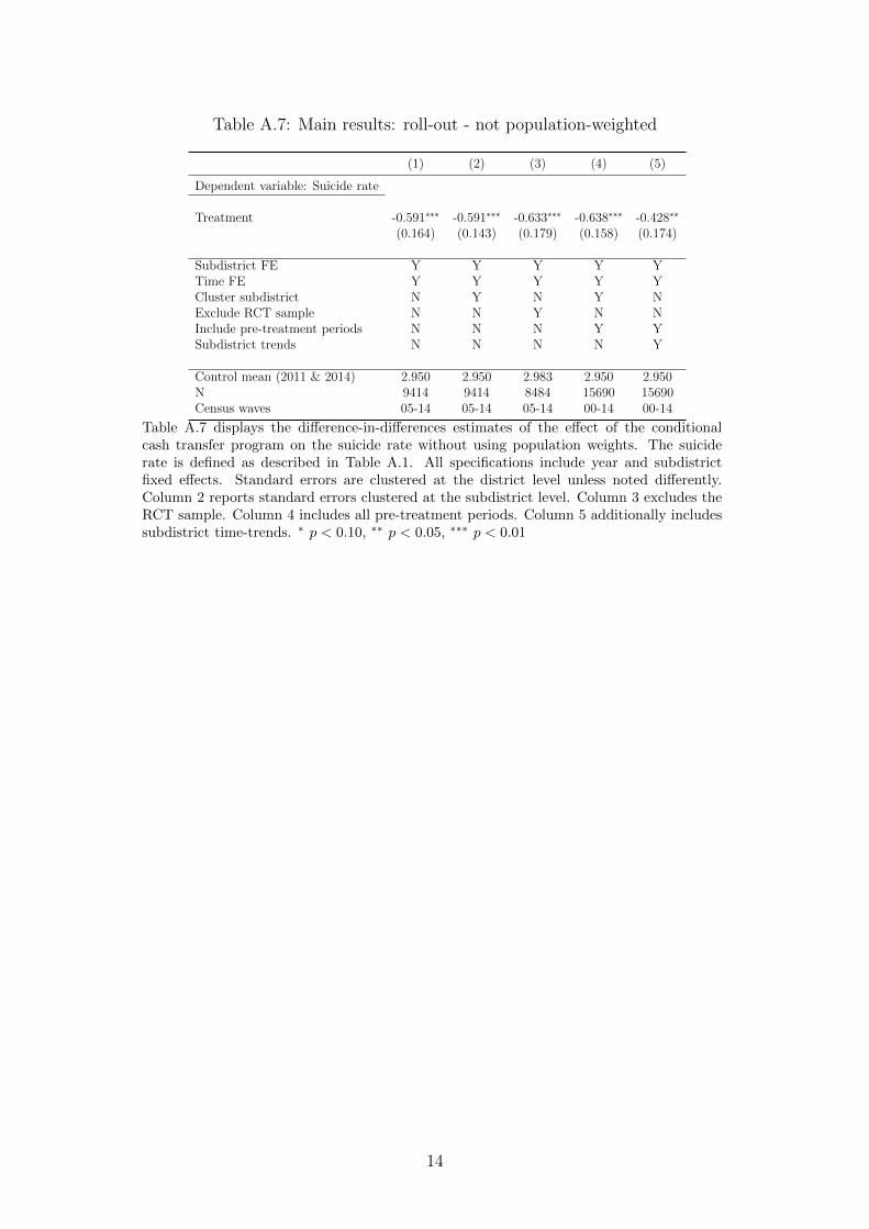
Table A.7: Main results: roll-out - not population-weighted

(1) (2) (3) (4) (5)

Dependent variable: Suicide rate

Treatment -0.591∗∗∗ -0.591∗∗∗ -0.633∗∗∗ -0.638∗∗∗ -0.428∗∗

(0.164) (0.143) (0.179) (0.158) (0.174)

Subdistrict FE Y Y Y Y YTime FE Y Y Y Y YCluster subdistrict N Y N Y NExclude RCT sample N N Y N NInclude pre-treatment periods N N N Y YSubdistrict trends N N N N Y

Control mean (2011 & 2014) 2.950 2.950 2.983 2.950 2.950N 9414 9414 8484 15690 15690Census waves 05-14 05-14 05-14 00-14 00-14

Table A.7 displays the difference-in-differences estimates of the effect of the conditionalcash transfer program on the suicide rate without using population weights. The suiciderate is defined as described in Table A.1. All specifications include year and subdistrictfixed effects. Standard errors are clustered at the district level unless noted differently.Column 2 reports standard errors clustered at the subdistrict level. Column 3 excludes theRCT sample. Column 4 includes all pre-treatment periods. Column 5 additionally includessubdistrict time-trends. ∗ p < 0.10, ∗∗ p < 0.05, ∗∗∗ p < 0.01

14

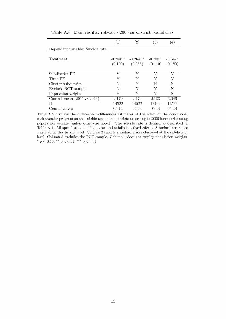
Table A.8: Main results: roll-out - 2006 subdistrict boundaries

(1) (2) (3) (4)

Dependent variable: Suicide rate

Treatment -0.264∗∗∗ -0.264∗∗∗ -0.255∗∗ -0.347∗

(0.102) (0.088) (0.110) (0.180)

Subdistrict FE Y Y Y YTime FE Y Y Y YCluster subdistrict N Y N NExclude RCT sample N N Y NPopulation weights Y Y Y NControl mean (2011 & 2014) 2.170 2.170 2.183 3.046N 14522 14522 13469 14522Census waves 05-14 05-14 05-14 05-14

Table A.8 displays the difference-in-differences estimates of the effect of the conditionalcash transfer program on the suicide rate in subdistricts according to 2006 boundaries usingpopulation weights (unless otherwise noted). The suicide rate is defined as described inTable A.1. All specifications include year and subdistrict fixed effects. Standard errors areclustered at the district level. Column 2 reports standard errors clustered at the subdistrictlevel. Column 3 excludes the RCT sample. Column 4 does not employ population weights.∗ p < 0.10, ∗∗ p < 0.05, ∗∗∗ p < 0.01

15

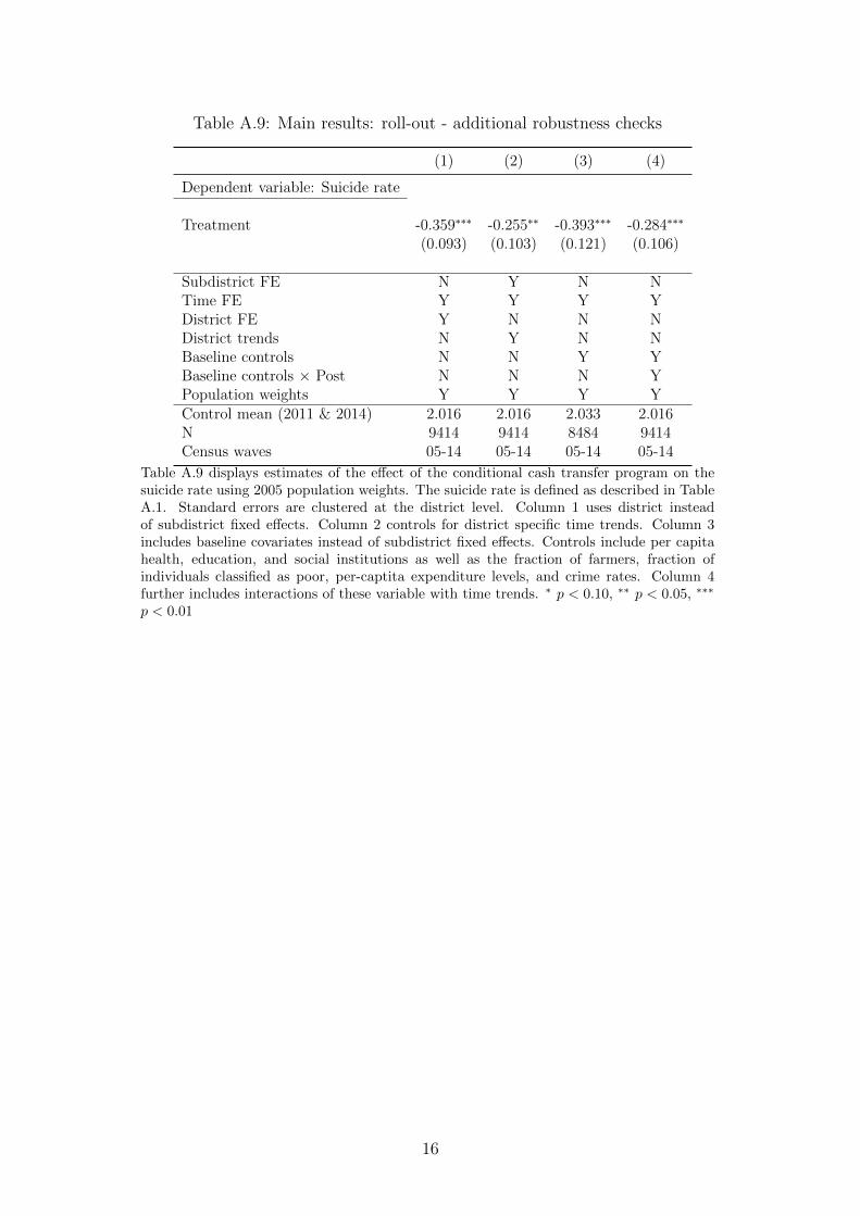
Table A.9: Main results: roll-out - additional robustness checks

(1) (2) (3) (4)

Dependent variable: Suicide rate

Treatment -0.359∗∗∗ -0.255∗∗ -0.393∗∗∗ -0.284∗∗∗

(0.093) (0.103) (0.121) (0.106)

Subdistrict FE N Y N NTime FE Y Y Y YDistrict FE Y N N NDistrict trends N Y N NBaseline controls N N Y YBaseline controls × Post N N N YPopulation weights Y Y Y YControl mean (2011 & 2014) 2.016 2.016 2.033 2.016N 9414 9414 8484 9414Census waves 05-14 05-14 05-14 05-14

Table A.9 displays estimates of the effect of the conditional cash transfer program on thesuicide rate using 2005 population weights. The suicide rate is defined as described in TableA.1. Standard errors are clustered at the district level. Column 1 uses district insteadof subdistrict fixed effects. Column 2 controls for district specific time trends. Column 3includes baseline covariates instead of subdistrict fixed effects. Controls include per capitahealth, education, and social institutions as well as the fraction of farmers, fraction ofindividuals classified as poor, per-captita expenditure levels, and crime rates. Column 4further includes interactions of these variable with time trends. ∗ p < 0.10, ∗∗ p < 0.05, ∗∗∗

p < 0.01

16

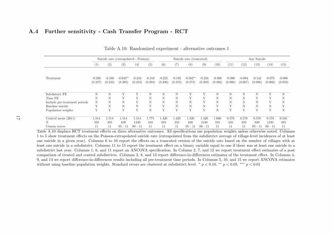
A.4 Further sensitivity - Cash Transfer Program - RCT

Table A.10: Randomized experiment - alternative outcomes 1

Suicide rate (extrapolated - Poisson) Suicide rate (truncated) Any Suicide

(1) (2) (3) (4) (5) (6) (7) (8) (9) (10) (11) (12) (13) (14) (15)

Treatment -0.236 -0.160 -0.633∗∗ -0.244 -0.318 -0.225 -0.192 -0.562∗∗ -0.224 -0.306 -0.096 -0.084 -0.142 -0.078 -0.086(0.227) (0.234) (0.305) (0.224) (0.294) (0.206) (0.253) (0.272) (0.203) (0.266) (0.066) (0.067) (0.086) (0.066) (0.059)

Subdistrict FE N N Y Y N N N Y Y N N N Y Y NTime FE N N Y Y N N N Y Y N N N Y Y NInclude pre-treatment periods N N N Y N N N N Y N N N N Y NBaseline suicide Y N N N Y Y N N N Y Y N N N YPopulation weights Y Y Y Y N Y Y Y Y N Y Y Y Y N

Control mean (2011) 1.514 1.514 1.514 1.514 1.775 1.420 1.420 1.420 1.420 1.666 0.578 0.578 0.578 0.578 0.545N 310 310 620 1240 310 310 310 620 1240 310 310 310 620 1240 310Census waves 11 11 05 - 11 00 - 11 11 11 11 05 - 11 00 - 11 11 11 11 05 - 11 00 - 11 11

Table A.10 displays RCT treatment effects on three alternative outcomes. All specifications use population weights unless otherwise noted. Columns1 to 5 show treatment effects on the Poisson-extrapolated suicide rate (extrapolated from the subdistrict average of village-level incidences of at leastone suicide in a given year). Columns 6 to 10 report the effects on a truncated version of the suicide rate based on the number of villages with atleast one suicide in a subdistrict. Columns 11 to 15 report the treatment effect on a binary variable equal to one if there was at least one suicide in asubdistrict last year. Columns 1, 6, and 11 report an ANCOVA specification. In Column 2, 7, and 12 we report treatment effect estimates of a postcomparison of treated and control subdistricts. Columns 3, 8, and 13 report difference-in-differences estimates of the treatment effect. In Columns 4,9, and 14 we report difference-in-differences results including all pre-treatment time periods. In Columns 5, 10, and 15 we report ANCOVA estimateswithout using baseline population weights. Standard errors are clustered at subdistrict level. ∗ p < 0.10, ∗∗ p < 0.05, ∗∗∗ p < 0.01

17

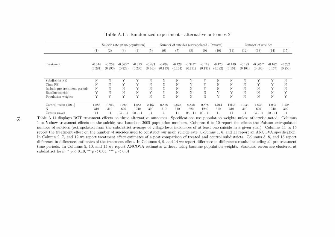
Table A.11: Randomized experiment - alternative outcomes 2

Suicide rate (2005 population) Number of suicides (extrapolated - Poisson) Number of suicides

(1) (2) (3) (4) (5) (6) (7) (8) (9) (10) (11) (12) (13) (14) (15)

Treatment -0.344 -0.256 -0.663∗∗ -0.313 -0.483 -0.099 -0.129 -0.345∗∗ -0.118 -0.170 -0.149 -0.129 -0.365∗∗ -0.167 -0.232(0.281) (0.293) (0.328) (0.280) (0.340) (0.133) (0.164) (0.171) (0.131) (0.182) (0.161) (0.164) (0.183) (0.157) (0.250)

Subdistrict FE N N Y Y N N N Y Y N N N Y Y NTime FE N N Y Y N N N Y Y N N N Y Y NInclude pre-treatment periods N N N Y N N N N Y N N N N Y NBaseline suicide Y N N N Y Y N N N Y Y N N N YPopulation weights Y Y Y Y N N N N N Y N N N N Y

Control mean (2011) 1.883 1.883 1.883 1.883 2.167 0.878 0.878 0.878 0.878 1.014 1.035 1.035 1.035 1.035 1.228N 310 310 620 1240 310 310 310 620 1240 310 310 310 620 1240 310Census waves 11 11 05 - 11 00 - 11 11 11 11 05 - 11 00 - 11 11 11 11 05 - 11 00 - 11 11

Table A.11 displays RCT treatment effects on three alternative outcomes. Specifications use population weights unless otherwise noted. Columns1 to 5 show treatment effects on the suicide rate based on 2005 population numbers. Columns 6 to 10 report the effects the Poisson extrapolatednumber of suicides (extrapolated from the subdistrict average of village-level incidences of at least one suicide in a given year). Columns 11 to 15report the treatment effect on the number of suicides used to construct our main suicide rate. Columns 1, 6, and 11 report an ANCOVA specification.In Column 2, 7, and 12 we report treatment effect estimates of a post comparison of treated and control subdistricts. Columns 3, 8, and 13 reportdifference-in-differences estimates of the treatment effect. In Columns 4, 9, and 14 we report difference-in-differences results including all pre-treatmenttime periods. In Columns 5, 10, and 15 we report ANCOVA estimates without using baseline population weights. Standard errors are clustered atsubdistrict level. ∗ p < 0.10, ∗∗ p < 0.05, ∗∗∗ p < 0.01

18

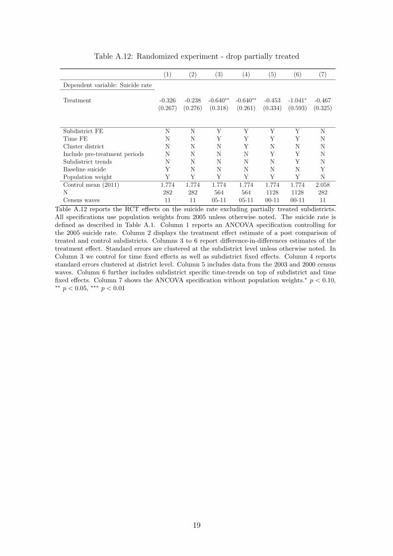
Table A.12: Randomized experiment - drop partially treated

(1) (2) (3) (4) (5) (6) (7)

Dependent variable: Suicide rate

Treatment -0.326 -0.238 -0.640∗∗ -0.640∗∗ -0.453 -1.041∗ -0.467(0.267) (0.276) (0.318) (0.261) (0.334) (0.593) (0.325)

Subdistrict FE N N Y Y Y Y NTime FE N N Y Y Y Y NCluster district N N N Y N N NInclude pre-treatment periods N N N N Y Y NSubdistrict trends N N N N N Y NBaseline suicide Y N N N N N YPopulation weight Y Y Y Y Y Y NControl mean (2011) 1.774 1.774 1.774 1.774 1.774 1.774 2.058N 282 282 564 564 1128 1128 282Census waves 11 11 05-11 05-11 00-11 00-11 11

Table A.12 reports the RCT effects on the suicide rate excluding partially treated subdistricts.All specifications use population weights from 2005 unless otherwise noted. The suicide rate isdefined as described in Table A.1. Column 1 reports an ANCOVA specification controlling forthe 2005 suicide rate. Column 2 displays the treatment effect estimate of a post comparison oftreated and control subdistricts. Columns 3 to 6 report difference-in-differences estimates of thetreatment effect. Standard errors are clustered at the subdistrict level unless otherwise noted. InColumn 3 we control for time fixed effects as well as subdistrict fixed effects. Column 4 reportsstandard errors clustered at district level. Column 5 includes data from the 2003 and 2000 censuswaves. Column 6 further includes subdistrict specific time-trends on top of subdistrict and timefixed effects. Column 7 shows the ANCOVA specification without population weights.∗ p < 0.10,∗∗ p < 0.05, ∗∗∗ p < 0.01

19

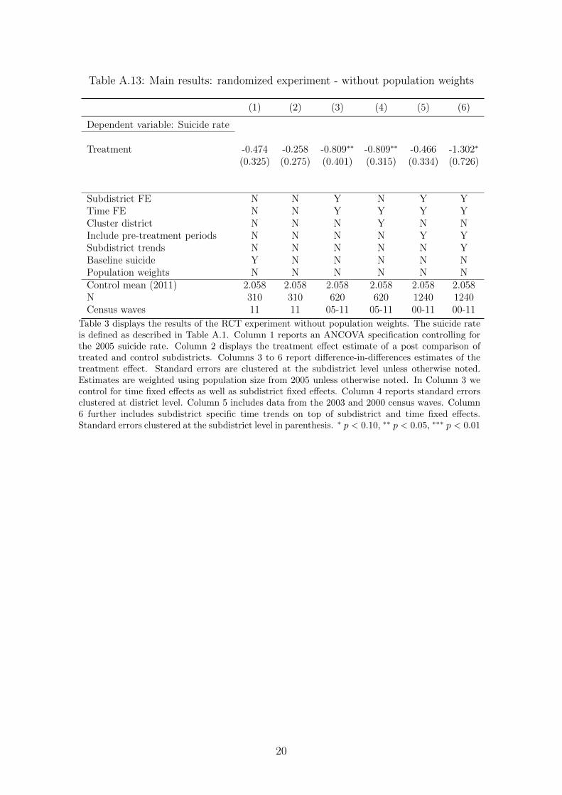
Table A.13: Main results: randomized experiment - without population weights

(1) (2) (3) (4) (5) (6)

Dependent variable: Suicide rate

Treatment -0.474 -0.258 -0.809∗∗ -0.809∗∗ -0.466 -1.302∗

(0.325) (0.275) (0.401) (0.315) (0.334) (0.726)

Subdistrict FE N N Y N Y YTime FE N N Y Y Y YCluster district N N N Y N NInclude pre-treatment periods N N N N Y YSubdistrict trends N N N N N YBaseline suicide Y N N N N NPopulation weights N N N N N NControl mean (2011) 2.058 2.058 2.058 2.058 2.058 2.058N 310 310 620 620 1240 1240Census waves 11 11 05-11 05-11 00-11 00-11

Table 3 displays the results of the RCT experiment without population weights. The suicide rateis defined as described in Table A.1. Column 1 reports an ANCOVA specification controlling forthe 2005 suicide rate. Column 2 displays the treatment effect estimate of a post comparison oftreated and control subdistricts. Columns 3 to 6 report difference-in-differences estimates of thetreatment effect. Standard errors are clustered at the subdistrict level unless otherwise noted.Estimates are weighted using population size from 2005 unless otherwise noted. In Column 3 wecontrol for time fixed effects as well as subdistrict fixed effects. Column 4 reports standard errorsclustered at district level. Column 5 includes data from the 2003 and 2000 census waves. Column6 further includes subdistrict specific time trends on top of subdistrict and time fixed effects.Standard errors clustered at the subdistrict level in parenthesis. ∗ p < 0.10, ∗∗ p < 0.05, ∗∗∗ p < 0.01

20

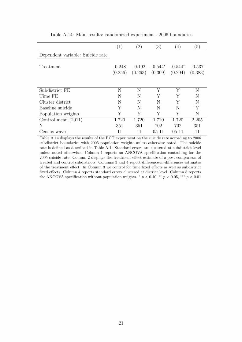
Table A.14: Main results: randomized experiment - 2006 boundaries

(1) (2) (3) (4) (5)

Dependent variable: Suicide rate

Treatment -0.248 -0.192 -0.544∗ -0.544∗ -0.537(0.256) (0.263) (0.309) (0.294) (0.383)

Subdistrict FE N N Y Y NTime FE N N Y Y NCluster district N N N Y NBaseline suicide Y N N N YPopulation weights Y Y Y Y NControl mean (2011) 1.720 1.720 1.720 1.720 2.205N 351 351 702 702 351Census waves 11 11 05-11 05-11 11

Table A.14 displays the results of the RCT experiment on the suicide rate according to 2006subdistrict boundaries with 2005 population weights unless otherwise noted. The suiciderate is defined as described in Table A.1. Standard errors are clustered at subdistrict levelunless noted otherwise. Column 1 reports an ANCOVA specification controlling for the2005 suicide rate. Column 2 displays the treatment effect estimate of a post comparison oftreated and control subdistricts. Columns 3 and 4 report difference-in-differences estimatesof the treatment effect. In Column 3 we control for time fixed effects as well as subdistrictfixed effects. Column 4 reports standard errors clustered at district level. Column 5 reportsthe ANCOVA specification without population weights. ∗ p < 0.10, ∗∗ p < 0.05, ∗∗∗ p < 0.01

21

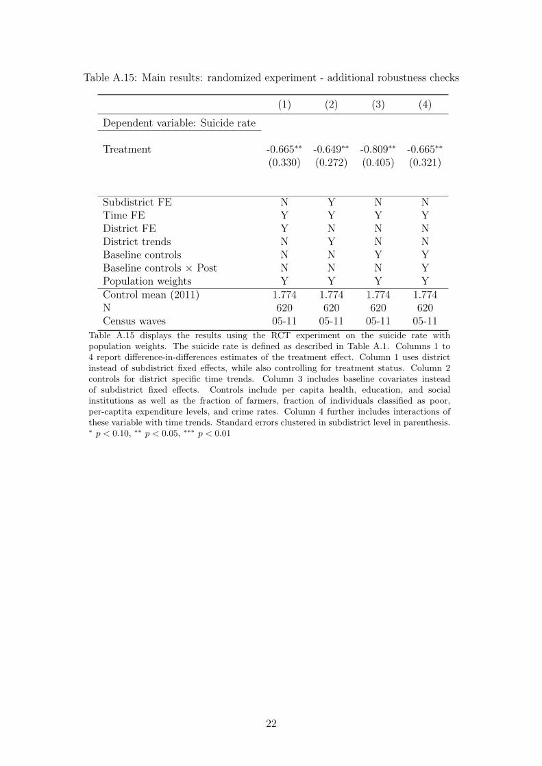
Table A.15: Main results: randomized experiment - additional robustness checks

(1) (2) (3) (4)

Dependent variable: Suicide rate

Treatment -0.665∗∗ -0.649∗∗ -0.809∗∗ -0.665∗∗

(0.330) (0.272) (0.405) (0.321)

Subdistrict FE N Y N NTime FE Y Y Y YDistrict FE Y N N NDistrict trends N Y N NBaseline controls N N Y YBaseline controls × Post N N N YPopulation weights Y Y Y YControl mean (2011) 1.774 1.774 1.774 1.774N 620 620 620 620Census waves 05-11 05-11 05-11 05-11

Table A.15 displays the results using the RCT experiment on the suicide rate withpopulation weights. The suicide rate is defined as described in Table A.1. Columns 1 to4 report difference-in-differences estimates of the treatment effect. Column 1 uses districtinstead of subdistrict fixed effects, while also controlling for treatment status. Column 2controls for district specific time trends. Column 3 includes baseline covariates insteadof subdistrict fixed effects. Controls include per capita health, education, and socialinstitutions as well as the fraction of farmers, fraction of individuals classified as poor,per-captita expenditure levels, and crime rates. Column 4 further includes interactions ofthese variable with time trends. Standard errors clustered in subdistrict level in parenthesis.∗ p < 0.10, ∗∗ p < 0.05, ∗∗∗ p < 0.01

22

A.5 Dynamics of treatment effects

23

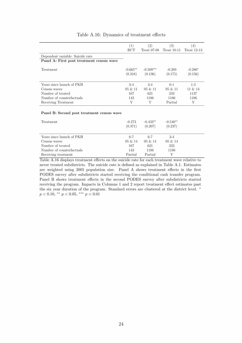
Table A.16: Dynamics of treatment effects

(1) (2) (3) (4)RCT Treat 07-08 Treat 10-11 Treat 12-13

Dependent variable: Suicide ratePanel A: First post treatment census wave

Treatment -0.665∗∗ -0.509∗∗∗ -0.289 -0.280∗

(0.318) (0.136) (0.175) (0.156)

Years since launch of PKH 3-4 3-4 0-1 1-2Census waves 05 & 11 05 & 11 05 & 11 11 & 14Number of treated 167 621 233 1137Number of counterfactuals 143 1186 1186 1186Receiving Treatment Y Y Partial Y

Panel B: Second post treatment census wave

Treatment -0.273 -0.433∗∗ -0.540∗∗

(0.371) (0.207) (0.237)

Years since launch of PKH 6-7 6-7 3-4Census waves 05 & 14 05 & 14 05 & 14Number of treated 167 621 233Number of counterfactuals 143 1186 1186Receiving treatment Partial Partial Y

Table A.16 displays treatment effects on the suicide rate for each treatment wave relative tonever treated subdistricts. The suicide rate is defined as explained in Table A.1. Estimatesare weighted using 2005 population size. Panel A shows treatment effects in the firstPODES survey after subdistricts started receiving the conditional cash transfer program.Panel B shows treatment effects in the second PODES survey after subdistricts startedreceiving the program. Impacts in Columns 1 and 2 report treatment effect estimates pastthe six year duration of the program. Standard errors are clustered at the district level. ∗

p < 0.10, ∗∗ p < 0.05, ∗∗∗ p < 0.01

24

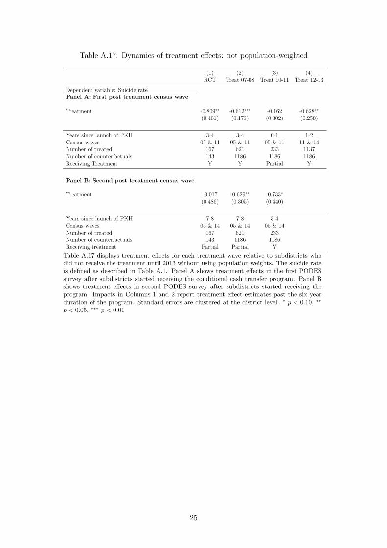
Table A.17: Dynamics of treatment effects: not population-weighted

(1) (2) (3) (4)RCT Treat 07-08 Treat 10-11 Treat 12-13

Dependent variable: Suicide ratePanel A: First post treatment census wave

Treatment -0.809∗∗ -0.612∗∗∗ -0.162 -0.628∗∗

(0.401) (0.173) (0.302) (0.259)

Years since launch of PKH 3-4 3-4 0-1 1-2Census waves 05 & 11 05 & 11 05 & 11 11 & 14Number of treated 167 621 233 1137Number of counterfactuals 143 1186 1186 1186Receiving Treatment Y Y Partial Y

Panel B: Second post treatment census wave

Treatment -0.017 -0.629∗∗ -0.733∗

(0.486) (0.305) (0.440)

Years since launch of PKH 7-8 7-8 3-4Census waves 05 & 14 05 & 14 05 & 14Number of treated 167 621 233Number of counterfactuals 143 1186 1186Receiving treatment Partial Partial Y

Table A.17 displays treatment effects for each treatment wave relative to subdistricts whodid not receive the treatment until 2013 without using population weights. The suicide rateis defined as described in Table A.1. Panel A shows treatment effects in the first PODESsurvey after subdistricts started receiving the conditional cash transfer program. Panel Bshows treatment effects in second PODES survey after subdistricts started receiving theprogram. Impacts in Columns 1 and 2 report treatment effect estimates past the six yearduration of the program. Standard errors are clustered at the district level. ∗ p < 0.10, ∗∗

p < 0.05, ∗∗∗ p < 0.01

25

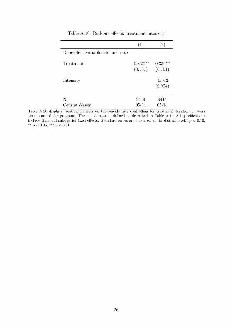
Table A.18: Roll-out effects: treatment intensity

(1) (2)

Dependent variable: Suicide rate

Treatment -0.358∗∗∗ -0.336∗∗∗

(0.101) (0.101)

Intensity -0.012(0.024)

N 9414 9414Census Waves 05-14 05-14

Table A.26 displays treatment effects on the suicide rate controlling for treatment duration in yearssince start of the program. The suicide rate is defined as described in Table A.1. All specificationsinclude time and subdistrict fixed effects. Standard errors are clustered at the district level.∗ p < 0.10,∗∗ p < 0.05, ∗∗∗ p < 0.01

26

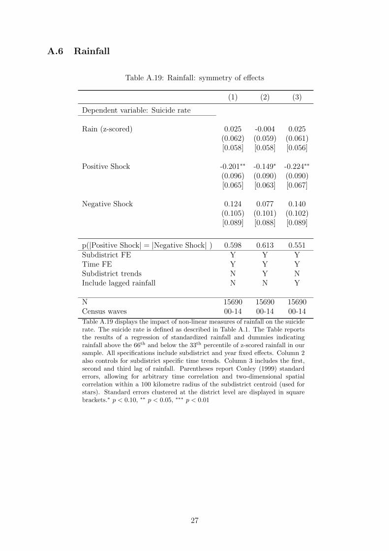
A.6 Rainfall

Table A.19: Rainfall: symmetry of effects

(1) (2) (3)

Dependent variable: Suicide rate

Rain (z-scored) 0.025 -0.004 0.025(0.062) (0.059) (0.061)[0.058] [0.058] [0.056]

Positive Shock -0.201∗∗ -0.149∗ -0.224∗∗

(0.096) (0.090) (0.090)[0.065] [0.063] [0.067]

Negative Shock 0.124 0.077 0.140(0.105) (0.101) (0.102)[0.089] [0.088] [0.089]

p(|Positive Shock| = |Negative Shock| ) 0.598 0.613 0.551Subdistrict FE Y Y YTime FE Y Y YSubdistrict trends N Y NInclude lagged rainfall N N Y

N 15690 15690 15690Census waves 00-14 00-14 00-14

Table A.19 displays the impact of non-linear measures of rainfall on the suiciderate. The suicide rate is defined as described in Table A.1. The Table reportsthe results of a regression of standardized rainfall and dummies indicatingrainfall above the 66th and below the 33th percentile of z-scored rainfall in oursample. All specifications include subdistrict and year fixed effects. Column 2also controls for subdistrict specific time trends. Column 3 includes the first,second and third lag of rainfall. Parentheses report Conley (1999) standarderrors, allowing for arbitrary time correlation and two-dimensional spatialcorrelation within a 100 kilometre radius of the subdistrict centroid (used forstars). Standard errors clustered at the district level are displayed in squarebrackets.∗ p < 0.10, ∗∗ p < 0.05, ∗∗∗ p < 0.01

27

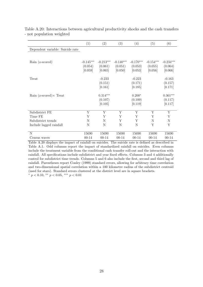
Table A.20: Interactions between agricultural productivity shocks and the cash transfers- not population weighted

(1) (2) (3) (4) (5) (6)

Dependent variable: Suicide rate

Rain (z-scored) -0.145∗∗∗ -0.213∗∗∗ -0.140∗∗∗ -0.170∗∗∗ -0.154∗∗∗ -0.234∗∗∗

(0.054) (0.061) (0.051) (0.053) (0.055) (0.064)[0.059] [0.065] [0.050] [0.053] [0.056] [0.066]

Treat -0.233 -0.223 -0.163(0.151) (0.171) (0.157)[0.161] [0.185] [0.171]

Rain (z-scored)× Treat 0.314∗∗∗ 0.200∗ 0.361∗∗∗

(0.107) (0.109) (0.117)[0.105] [0.119] [0.117]

Subdistrict FE Y Y Y Y Y YTime FE Y Y Y Y Y YSubdistrict trends N N Y Y N NInclude lagged rainfall N N N N Y Y

N 15690 15690 15690 15690 15690 15690Census waves 00-14 00-14 00-14 00-14 00-14 00-14

Table A.20 displays the impact of rainfall on suicides. The suicide rate is defined as described inTable A.1. Odd columns report the impact of standardized rainfall on suicides. Even columnsinclude the treatment variable from the conditional cash transfer roll-out and the interaction withrainfall. All specifications include subdistrict and year fixed effects. Columns 3 and 4 additionallycontrol for subdistrict time trends. Columns 5 and 6 also include the first, second and third lag ofrainfall. Parentheses report Conley (1999) standard errors, allowing for arbitrary time correlationand two-dimensional spatial correlation within a 100 kilometre radius of the subdistrict centroid(used for stars). Standard errors clustered at the district level are in square brackets.∗ p < 0.10, ∗∗ p < 0.05, ∗∗∗ p < 0.01

28

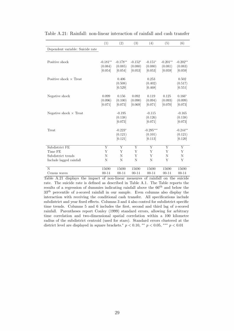
Table A.21: Rainfall: non-linear interaction of rainfall and cash transfer

(1) (2) (3) (4) (5) (6)

Dependent variable: Suicide rate

Positive shock -0.181∗∗ -0.178∗∗ -0.152∗ -0.151∗ -0.201∗∗ -0.202∗∗

(0.084) (0.085) (0.080) (0.080) (0.081) (0.083)[0.054] [0.054] [0.053] [0.053] [0.059] [0.059]

Positive shock × Treat 0.406 0.253 0.502(0.508) (0.402) (0.517)[0.529] [0.468] [0.551]

Negative shock 0.099 0.156 0.092 0.119 0.125 0.166∗

(0.096) (0.100) (0.090) (0.094) (0.093) (0.099)[0.071] [0.073] [0.069] [0.071] [0.070] [0.073]

Negative shock × Treat -0.195 -0.115 -0.165(0.138) (0.126) (0.138)[0.073] [0.071] [0.073]

Treat -0.223∗ -0.295∗∗∗ -0.244∗∗

(0.121) (0.101) (0.121)[0.121] [0.113] [0.120]

Subdistrict FE Y Y Y Y Y YTime FE Y Y Y Y Y YSubdistrict trends N N Y Y N NInclude lagged rainfall N N N N Y Y

N 15690 15690 15690 15690 15690 15690Census waves 00-14 00-14 00-14 00-14 00-14 00-14

Table A.21 displays the impact of non-linear measures of rainfall on the suiciderate. The suicide rate is defined as described in Table A.1. The Table reports theresults of a regression of dummies indicating rainfall above the 66th and below the33th percentile of z-scored rainfall in our sample. Even columns also display theinteraction with receiving the conditional cash transfer. All specifications includesubdistrict and year fixed effects. Columns 3 and 4 also control for subdistrict specifictime trends. Columns 5 and 6 includes the first, second and third lag of z-scoredrainfall. Parentheses report Conley (1999) standard errors, allowing for arbitrarytime correlation and two-dimensional spatial correlation within a 100 kilometreradius of the subdistrict centroid (used for stars). Standard errors clustered at thedistrict level are displayed in square brackets.∗ p < 0.10, ∗∗ p < 0.05, ∗∗∗ p < 0.01

29

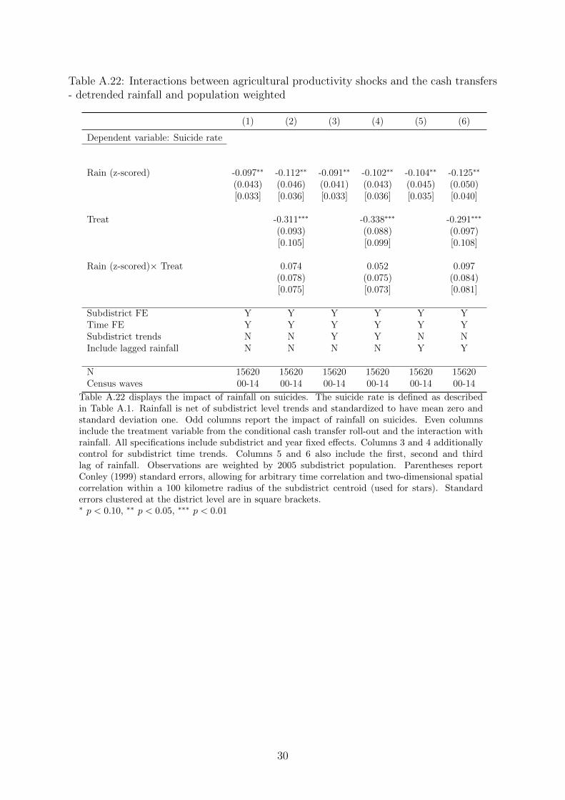
Table A.22: Interactions between agricultural productivity shocks and the cash transfers- detrended rainfall and population weighted

(1) (2) (3) (4) (5) (6)

Dependent variable: Suicide rate

Rain (z-scored) -0.097∗∗ -0.112∗∗ -0.091∗∗ -0.102∗∗ -0.104∗∗ -0.125∗∗

(0.043) (0.046) (0.041) (0.043) (0.045) (0.050)[0.033] [0.036] [0.033] [0.036] [0.035] [0.040]

Treat -0.311∗∗∗ -0.338∗∗∗ -0.291∗∗∗

(0.093) (0.088) (0.097)[0.105] [0.099] [0.108]

Rain (z-scored)× Treat 0.074 0.052 0.097(0.078) (0.075) (0.084)[0.075] [0.073] [0.081]

Subdistrict FE Y Y Y Y Y YTime FE Y Y Y Y Y YSubdistrict trends N N Y Y N NInclude lagged rainfall N N N N Y Y

N 15620 15620 15620 15620 15620 15620Census waves 00-14 00-14 00-14 00-14 00-14 00-14

Table A.22 displays the impact of rainfall on suicides. The suicide rate is defined as describedin Table A.1. Rainfall is net of subdistrict level trends and standardized to have mean zero andstandard deviation one. Odd columns report the impact of rainfall on suicides. Even columnsinclude the treatment variable from the conditional cash transfer roll-out and the interaction withrainfall. All specifications include subdistrict and year fixed effects. Columns 3 and 4 additionallycontrol for subdistrict time trends. Columns 5 and 6 also include the first, second and thirdlag of rainfall. Observations are weighted by 2005 subdistrict population. Parentheses reportConley (1999) standard errors, allowing for arbitrary time correlation and two-dimensional spatialcorrelation within a 100 kilometre radius of the subdistrict centroid (used for stars). Standarderrors clustered at the district level are in square brackets.∗ p < 0.10, ∗∗ p < 0.05, ∗∗∗ p < 0.01

30

Table A.23: Interactions between agricultural productivity shocks and the cash transfers- detrended and not population weighted

(1) (2) (3) (4) (5) (6)

Dependent variable: Suicide rate

Rain (z-scored) -0.149∗∗∗ -0.194∗∗∗ -0.139∗∗ -0.175∗∗∗ -0.162∗∗∗ -0.217∗∗∗

(0.057) (0.060) (0.056) (0.058) (0.059) (0.064)[0.050] [0.055] [0.049] [0.053] [0.049] [0.057]

Treat -0.414∗∗∗ -0.479∗∗∗ -0.376∗∗∗

(0.128) (0.127) (0.130)[0.147] [0.142] [0.150]

Rain (z-scored)× Treat 0.256∗∗ 0.204∗ 0.301∗∗

(0.110) (0.108) (0.118)[0.107] [0.106] [0.117]

Subdistrict FE Y Y Y Y Y YTime FE Y Y Y Y Y YSubdistrict trends N N Y Y N NInclude lagged rainfall N N N N Y Y

N 15620 15620 15620 15620 15620 15620Census waves 00-14 00-14 00-14 00-14 00-14 00-14

Table A.23 displays the impact of rainfall on suicides. The suicide rate is defined as describedin Table A.1. Rainfall is net of subdistrict level trends and standardized to have mean zero andstandard deviation one. Odd columns report the impact of rainfall on suicides. Even columnsinclude the treatment variable from the conditional cash transfer roll-out and the interaction withrainfall. All specifications include subdistrict and year fixed effects. Columns 3 and 4 additionallycontrol for subdistrict time trends. Columns 5 and 6 also include the first, second and third lag ofrainfall. Parentheses report Conley (1999) standard errors, allowing for arbitrary time correlationand two-dimensional spatial correlation within a 100 kilometre radius of the subdistrict centroid(used for stars). Standard errors clustered at the district level are in square brackets.∗ p < 0.10, ∗∗ p < 0.05, ∗∗∗ p < 0.01

31

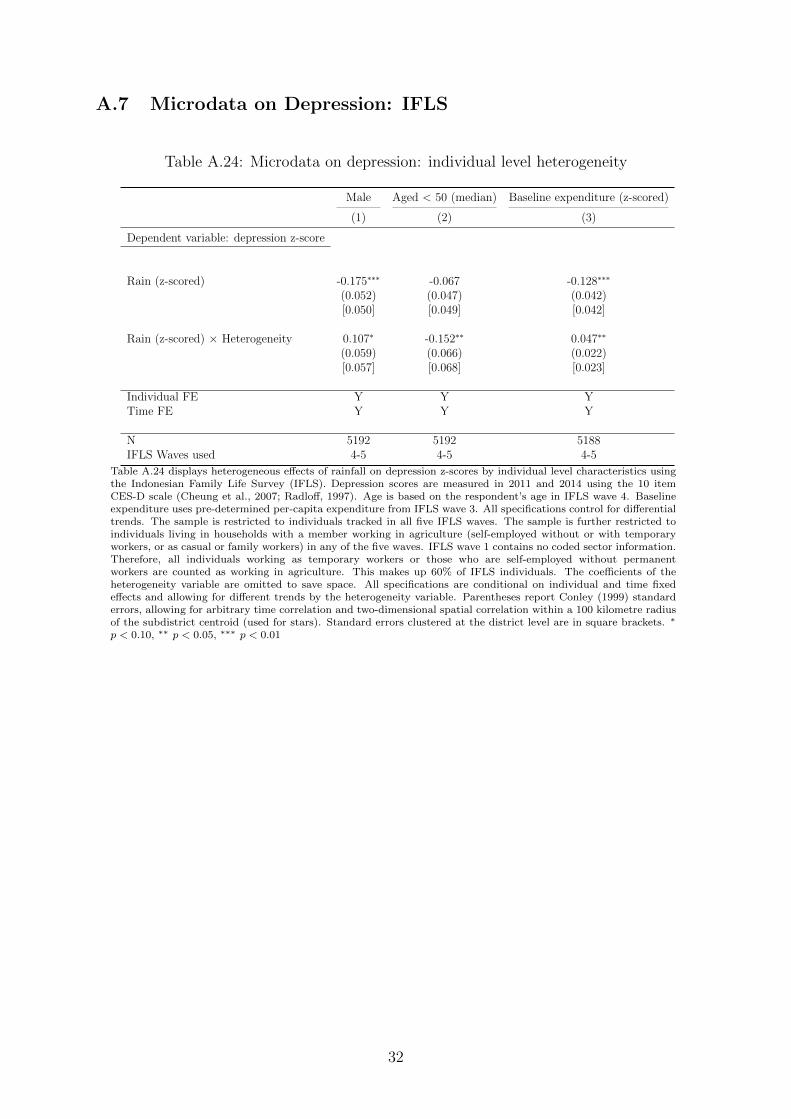
A.7 Microdata on Depression: IFLS

Table A.24: Microdata on depression: individual level heterogeneity

Male Aged < 50 (median) Baseline expenditure (z-scored)

(1) (2) (3)

Dependent variable: depression z-score

Rain (z-scored) -0.175∗∗∗ -0.067 -0.128∗∗∗

(0.052) (0.047) (0.042)[0.050] [0.049] [0.042]

Rain (z-scored) × Heterogeneity 0.107∗ -0.152∗∗ 0.047∗∗

(0.059) (0.066) (0.022)[0.057] [0.068] [0.023]

Individual FE Y Y YTime FE Y Y Y

N 5192 5192 5188IFLS Waves used 4-5 4-5 4-5

Table A.24 displays heterogeneous effects of rainfall on depression z-scores by individual level characteristics usingthe Indonesian Family Life Survey (IFLS). Depression scores are measured in 2011 and 2014 using the 10 itemCES-D scale (Cheung et al., 2007; Radloff, 1997). Age is based on the respondent’s age in IFLS wave 4. Baselineexpenditure uses pre-determined per-capita expenditure from IFLS wave 3. All specifications control for differentialtrends. The sample is restricted to individuals tracked in all five IFLS waves. The sample is further restricted toindividuals living in households with a member working in agriculture (self-employed without or with temporaryworkers, or as casual or family workers) in any of the five waves. IFLS wave 1 contains no coded sector information.Therefore, all individuals working as temporary workers or those who are self-employed without permanentworkers are counted as working in agriculture. This makes up 60% of IFLS individuals. The coefficients of theheterogeneity variable are omitted to save space. All specifications are conditional on individual and time fixedeffects and allowing for different trends by the heterogeneity variable. Parentheses report Conley (1999) standarderrors, allowing for arbitrary time correlation and two-dimensional spatial correlation within a 100 kilometre radiusof the subdistrict centroid (used for stars). Standard errors clustered at the district level are in square brackets. ∗

p < 0.10, ∗∗ p < 0.05, ∗∗∗ p < 0.01

32

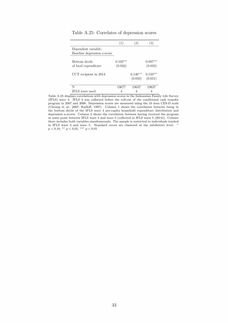
Table A.25: Correlates of depression scores

(1) (2) (3)

Dependent variable:Baseline depression z-score

Bottom decile 0.102∗∗∗ 0.097∗∗∗

of food expenditure (0.032) (0.033)

CCT recipient in 2014 0.146∗∗∗ 0.133∗∗∗

(0.050) (0.051)

N 19677 19637 19637IFLS wave used 4 4 4

Table A.25 displays correlations with depression scores in the Indonesian Family Life Survey(IFLS) wave 4. IFLS 4 was collected before the roll-out of the conditional cash transferprogram in 2007 and 2008. Depression scores are measured using the 10 item CES-D scale(Cheung et al., 2007; Radloff, 1997). Column 1 shows the correlation between being inthe bottom decile of the IFLS wave 4 per-capita household expenditure distribution anddepression z-scores. Column 2 shows the correlation between having received the programat some point between IFLS wave 4 and wave 5 (collected in IFLS wave 5 (2014)). Columnthree includes both variables simultaneously. The sample is restricted to individuals trackedin IFLS wave 4 and wave 5. Standard errors are clustered at the subdistrict level. ∗

p < 0.10, ∗∗ p < 0.05, ∗∗∗ p < 0.01

33

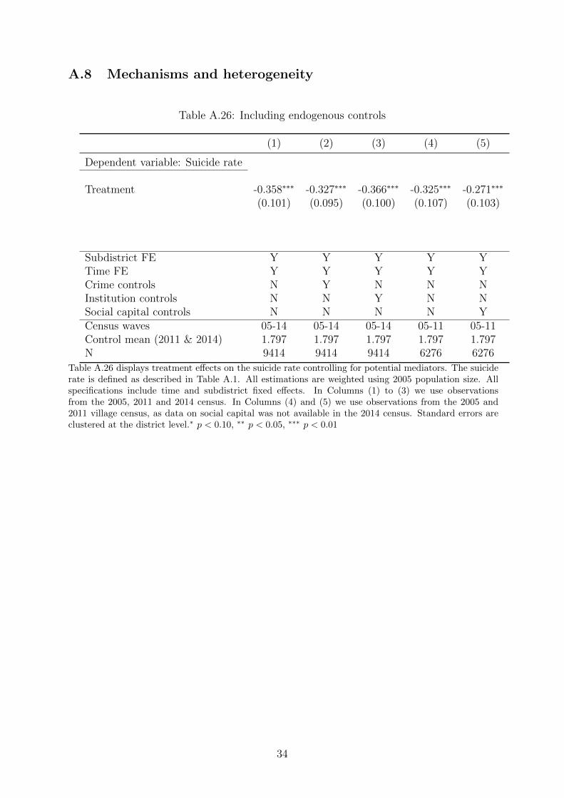
A.8 Mechanisms and heterogeneity

Table A.26: Including endogenous controls

(1) (2) (3) (4) (5)

Dependent variable: Suicide rate

Treatment -0.358∗∗∗ -0.327∗∗∗ -0.366∗∗∗ -0.325∗∗∗ -0.271∗∗∗

(0.101) (0.095) (0.100) (0.107) (0.103)

Subdistrict FE Y Y Y Y YTime FE Y Y Y Y YCrime controls N Y N N NInstitution controls N N Y N NSocial capital controls N N N N YCensus waves 05-14 05-14 05-14 05-11 05-11Control mean (2011 & 2014) 1.797 1.797 1.797 1.797 1.797N 9414 9414 9414 6276 6276

Table A.26 displays treatment effects on the suicide rate controlling for potential mediators. The suiciderate is defined as described in Table A.1. All estimations are weighted using 2005 population size. Allspecifications include time and subdistrict fixed effects. In Columns (1) to (3) we use observationsfrom the 2005, 2011 and 2014 census. In Columns (4) and (5) we use observations from the 2005 and2011 village census, as data on social capital was not available in the 2014 census. Standard errors areclustered at the district level.∗ p < 0.10, ∗∗ p < 0.05, ∗∗∗ p < 0.01

34

Table A.27: Subdistrict level heterogeneous treatment effects

(1) (2) (3) (4) (5) (6) (7)

Dependent variable: Suicide rate

Treatment -0.234 -0.357∗∗∗ -0.356∗∗∗ -0.380∗∗∗ -0.346∗∗∗ -0.283∗∗ -0.274∗

(0.147) (0.101) (0.113) (0.103) (0.108) (0.139) (0.145)

Treatment × 0.218∗ 0.122Fract poor (z) (0.122) (0.095)

Treatment × -0.105 -0.117Perc. Farmers (z) (0.102) (0.072)

Treatment × 0.120 0.026Per Capita Excp (z) (0.086) (0.059)

Treatment × 0.145 0.077Per Capita Crimes (z) (0.218) (0.183)

Treatment × 0.277 0.015Per Capita Social Institutions (z) (0.198) (0.191)

Treatment × -0.244 -0.127Per Capita Health Institutions (z) (0.256) (0.223)

Minimum detectable effect size 0.266 0.202 0.165 0.512 0.535 0.624N 9414 9414 9414 9414 9414 9414 9414Census waves 05-14 05-14 05-14 05-14 05-14 05-14 05-14

Table A.27 displays heterogeneous treatment effects on the suicide rate for the cash transfer roll-out bybaseline district level characteristics. The suicide rate is defined as described in Table A.1. All specifica-tion include time and subdistrict fixed effects. All estimations are weighted using 2005 population size.All interaction term variables, interactsd, are based on the 2005 census, and are z-scored using the meanand standard deviation of the sample. All specifications control for differential trends by interactionvariables, interactsd × postt, where post is defined as post-baseline years. “Minimum detectable effectsize” provides us with the minimum detectable effect size at 0.8 power and significance levels of 0.05for heterogeneous treatment effects for the different interactions variables. Estimates are based onyears 2005 to 2014. Standard errors are clustered at the district level. ∗ p < 0.10, ∗∗ p < 0.05, ∗∗∗ p < 0.01

35

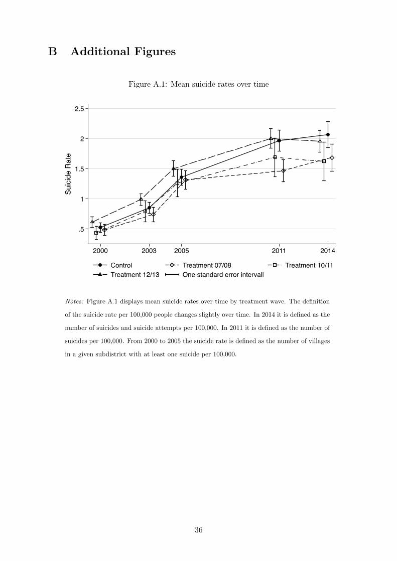
B Additional Figures

Figure A.1: Mean suicide rates over time

.5

1

1.5

2

2.5

Suici

de R

ate

2000 2003 2005 2011 2014

Control Treatment 07/08 Treatment 10/11Treatment 12/13 One standard error intervall

Notes: Figure A.1 displays mean suicide rates over time by treatment wave. The definition

of the suicide rate per 100,000 people changes slightly over time. In 2014 it is defined as the

number of suicides and suicide attempts per 100,000. In 2011 it is defined as the number of

suicides per 100,000. From 2000 to 2005 the suicide rate is defined as the number of villages

in a given subdistrict with at least one suicide per 100,000.

36

Figure A.2: Mean suicide rates by treatment group over time – not population-weighted

0

1

2

3

4

Suic

ide

Rat

e

2000 2003 2005 2011 2014

Control Treatment 07/08 Treatment 10/11Treatment 12/13 One standard error intervall

Notes: Figure A.2 displays mean suicide rates over time by treatment wave without population weights. The suicide rateis defined as in Figure A.1.

37

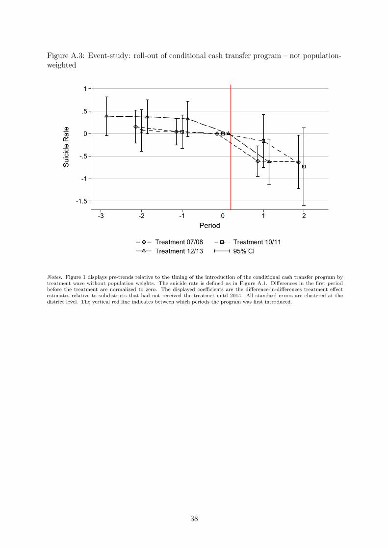
Figure A.3: Event-study: roll-out of conditional cash transfer program – not population-weighted

-1.5

-1

-.5

0

.5

1

Suic

ide

Rat

e

-3 -2 -1 0 1 2Period

Treatment 07/08 Treatment 10/11Treatment 12/13 95% CI

Notes: Figure 1 displays pre-trends relative to the timing of the introduction of the conditional cash transfer program bytreatment wave without population weights. The suicide rate is defined as in Figure A.1. Differences in the first periodbefore the treatment are normalized to zero. The displayed coefficients are the difference-in-differences treatment effectestimates relative to subdistricts that had not received the treatmet until 2014. All standard errors are clustered at thedistrict level. The vertical red line indicates between which periods the program was first introduced.

38

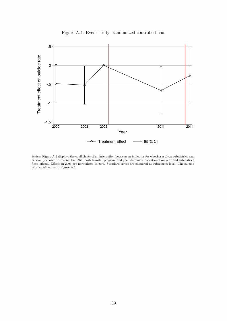
Figure A.4: Event-study: randomized controlled trial

-1.5

-1

-.5

0

.5

Trea

tmen

t effe

ct o

n su

icid

e ra

te

2000 2003 2005 2011 2014Year

Treatment Effect 95 % CI

Notes: Figure A.4 displays the coefficients of an interaction between an indicator for whether a given subdistrict wasrandomly chosen to receive the PKH cash transfer program and year dummies, conditional on year and subdistrictfixed effects. Effects in 2005 are normalized to zero. Standard errors are clustered at subdistrict level. The suiciderate is defined as in Figure A.1.

39

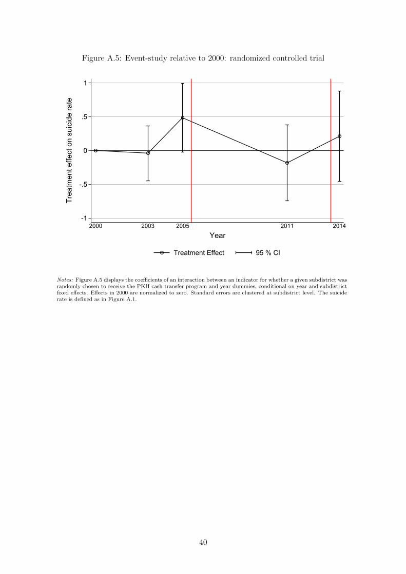
Figure A.5: Event-study relative to 2000: randomized controlled trial

-1

-.5

0

.5

1

Trea

tmen

t effe

ct o

n su

icid

e ra

te

2000 2003 2005 2011 2014

Year

Treatment Effect 95 % CI

Notes: Figure A.5 displays the coefficients of an interaction between an indicator for whether a given subdistrict wasrandomly chosen to receive the PKH cash transfer program and year dummies, conditional on year and subdistrictfixed effects. Effects in 2000 are normalized to zero. Standard errors are clustered at subdistrict level. The suiciderate is defined as in Figure A.1.

40

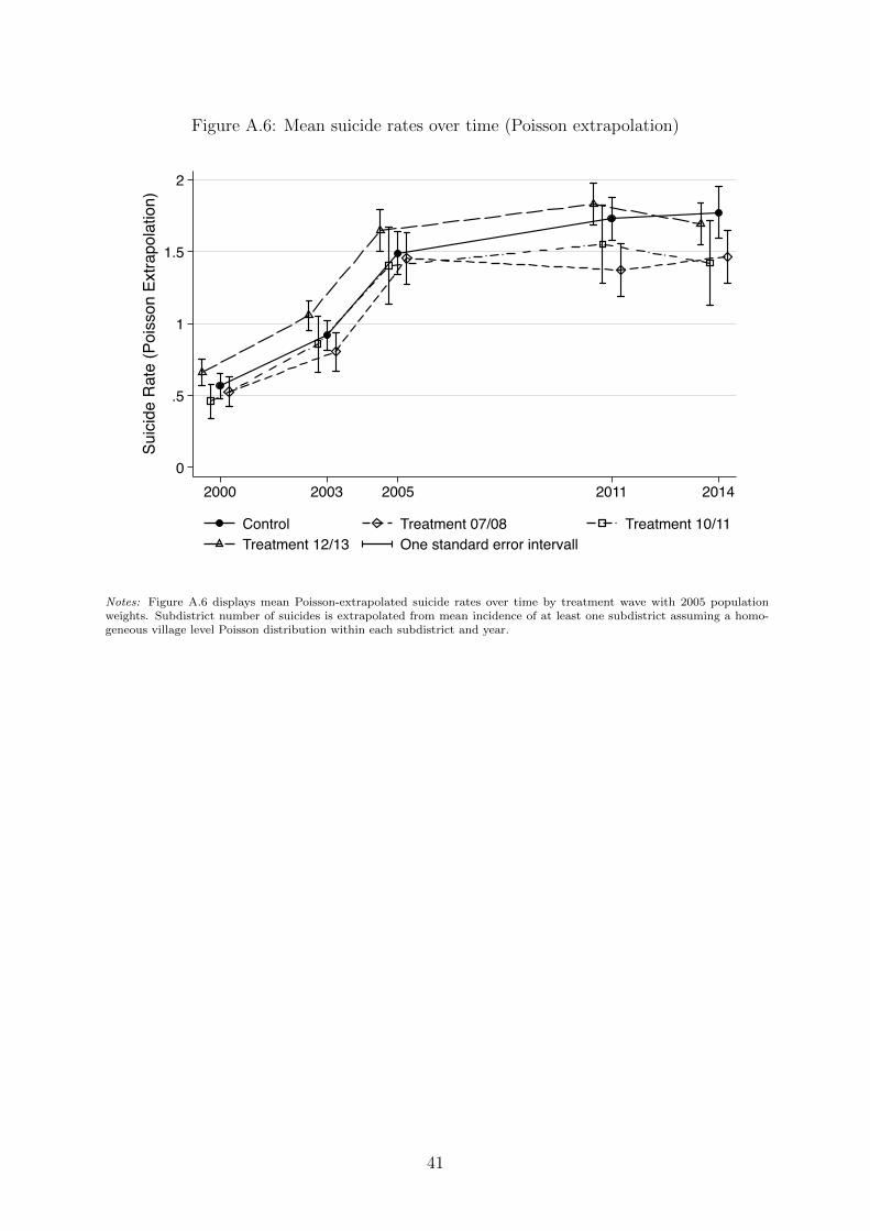
Figure A.6: Mean suicide rates over time (Poisson extrapolation)

0

.5

1

1.5

2

Suici

de R

ate

(Poi

sson

Ext

rapo

latio

n)

2000 2003 2005 2011 2014

Control Treatment 07/08 Treatment 10/11Treatment 12/13 One standard error intervall

Notes: Figure A.6 displays mean Poisson-extrapolated suicide rates over time by treatment wave with 2005 populationweights. Subdistrict number of suicides is extrapolated from mean incidence of at least one subdistrict assuming a homo-geneous village level Poisson distribution within each subdistrict and year.

41

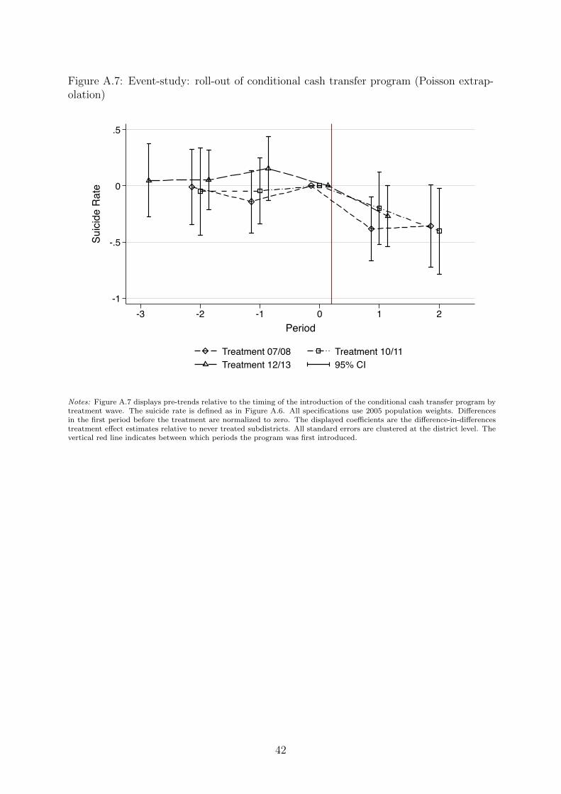
Figure A.7: Event-study: roll-out of conditional cash transfer program (Poisson extrap-olation)

-1

-.5

0

.5

Suic

ide

Rat

e

-3 -2 -1 0 1 2Period

Treatment 07/08 Treatment 10/11Treatment 12/13 95% CI

Notes: Figure A.7 displays pre-trends relative to the timing of the introduction of the conditional cash transfer program bytreatment wave. The suicide rate is defined as in Figure A.6. All specifications use 2005 population weights. Differencesin the first period before the treatment are normalized to zero. The displayed coefficients are the difference-in-differencestreatment effect estimates relative to never treated subdistricts. All standard errors are clustered at the district level. Thevertical red line indicates between which periods the program was first introduced.

42