INCOMPLETE LU PRECONDITIONER BASED ON

SIAM J. MATRIX ANAL. APPL. c© 2017 SIAM. Published by SIAM under the termsVol. 38, No. 4, pp. 1160–1189 of the Creative Commons 4.0 license

INCOMPLETE LU PRECONDITIONER BASED ONMAX-PLUS APPROXIMATION OF LU FACTORIZATION∗

JAMES HOOK† AND FRANCOISE TISSEUR‡

Abstract. We present a new method for the a priori approximation of the orders of magnitude ofthe entries in the LU factors of a complex or real matrix A. This approximation is used to determinethe positions of the largest entries in the LU factors of A, and these positions are used as the sparsitypattern for an incomplete LU factorization preconditioner. Our method uses max-plus algebra andis based solely on the moduli of the entries of A. We also present techniques for predicting whichpermutation matrices will be chosen by Gaussian elimination with partial pivoting. We exploit thestrong connection between the field of Puiseux series and the max-plus semiring to prove propertiesof the max-plus LU factors. Experiments with a set of test matrices from the University of FloridaSparse Matrix Collection show that our max-plus LU preconditioners outperform traditional level offill methods and have similar performance to those preconditioners computed with more expensivethreshold-based methods.

Key words. max-plus algebra, LU factorization, Hungarian scaling, linear systems of equations,sparse matrices, incomplete LU factorization, preconditioning

AMS subject classifications. 65F08, 65F30, 15A23, 15A80

DOI. 10.1137/16M1094579

1. Introduction. Max-plus algebra is the analogue of linear algebra developedfor the binary operations max and plus over the real numbers together with −∞,the latter playing the role of additive identity. Max-plus algebraic techniques havealready been used in numerical linear algebra to, for example, approximate the ordersof magnitude of the roots of scalar polynomials [19], approximate the moduli of theeigenvalues of matrix polynomials [1, 10, 14], and approximate singular values [9].These approximations have been used as starting points for iterative schemes andin the design of preprocessing steps to improve the numerical stability of standardalgorithms [3, 6, 7, 14, 20]. Our aim is to show how max-plus algebra can be usedto approximate the sizes of the entries in the LU factors of a complex or real matrixA and how these approximations can subsequently be used in the construction of anincomplete LU (ILU) factorization preconditioner for A.

In order to be able to apply max-plus techniques to the matrix A ∈ Cn×n wemust first transform it into a max-plus matrix. We do this using the valuation map

(1) Vc : C→ R := R ∪ {−∞}, Vc(x) = log |x| (log 0 = −∞).

The valuation map is applied to matrices componentwise, so that Vc(A) ∈ Rn×n is amax-plus matrix. Note that for x, y ∈ C, Vc(xy) = Vc(x) + Vc(y), and when |x| � |y|or |x| � |y|, then Vc(x+ y) ≈ max{Vc(x),Vc(y)}. This suggests using the operations

∗Received by the editors September 19, 2016; accepted for publication (in revised form) by D. B.Szyld August 21, 2017; published electronically October 19, 2017.

http://www.siam.org/journals/simax/38-4/M109457.htmlFunding: This work was supported by Engineering and Physical Sciences Research Council

grant EP/I005293. The work of the second author was also supported by a Royal Society-WolfsonResearch Merit Award.†Bath Institute for Mathematical Innovation, University of Bath, Bath BA2 7AY, UK (j.l.hook@

bath.ac.uk).‡School of Mathematics, The University of Manchester, Manchester M13 9PL, UK (francoise.

[email protected]).

1160

c© 2017 SIAM. Published by SIAM under the terms of the Creative Commons 4.0 license

Dow

nloa

ded

10/3

1/17

to 1

30.8

8.16

.37.

Red

istr

ibut

ion

subj

ect t

o C

CB

Y li

cens

e

http://www.siam.org/journals/simax/38-4/M109457.html

mailto:[email protected]




MAX-PLUS INCOMPLETE LU PRECONDITIONER 1161

max and plus, which we denote by ⊕ and ⊗, respectively, in place of the classicaladdition and multiplication once we have applied the map Vc.

The fundamental basis for our approximation of the magnitude of the entries ofthe LU factors of A ∈ Cn×n is

(a) the fact that the entries in the lower triangle of L and the upper triangle ofU can be expressed explicitly in terms of determinants of submatrices S ofA, and

(b) the heuristic that, when the matrix S has large variation in the size of itsentries, Vc(det(S)) ≈ perm(Vc(S)), where perm is the max-plus permanent.

We use (a) and (b) to define a lower triangular max-plus matrix L and an uppertriangular max-plus matrix U such that

(2) Vc(L) ≈ L, Vc(U) ≈ U ,

and we refer to L and U as the max-plus LU factors of A := Vc(A) ∈ Rn×n. Theapproximation (2) is a heuristic which only aims to capture the order of magnitude ofthe entries of L and U . One way to think about the max-plus LU approximation of theLU factors of A is as an intermediate between the true LU factors of A and a symbolicor Boolean factorization which, based purely on the pattern of nonzero entries in A,predicts the nonzero patterns of the LU factors. We show that the matrix-matrixproduct L⊗U is usually not a factorization of A but that it “balances” A, in a sensemade precise below.

In order for the max-plus approximation to be useful in practice, it is essentialthat the cost of computing it be less than the cost of computing the LU factorizationexactly. We show that the max-plus LU factors can be computed by solving maximallyweighted tree problems. As a result we provide an algorithm for computing the LUapproximation of A ∈ Cn×n with worst case cost O(nτ + n2 log n), where τ is thenumber of nonzero entries in A. Note that this cost depends on the number of nonzeroentries in A and not on the number of nonzero entries in the LU factors of A. Thuswhile the approximate LU factors will exhibit fill-in just as in the exact case, the costof computing the approximation is not affected by fill-in and will therefore be less thanthat of computing the exact LU factors. If the matrix A is first reordered accordingto its optimal assignment, so that the product of the moduli of the entries on itsdiagonal is maximized, then our approximation of the LU factors can be computed inparallel by n separate computations, each of individual cost O(τ +n log n). If we seekonly the positions and values of the k largest entries in each row of U and column ofL, or if we seek only the position and values of the entries that are greater in modulusthan some threshold, then this cost can be reduced further.

An approximation of the size of the entries in the LU factors of a sparse matrixA can be used to help construct an ILU preconditioner for solving Ax = b, that is, apair of sparse lower- and upper triangular matrices L,U such that the preconditionedmatrix AU−1L−1 is more amenable to iterative methods such as GMRES [17]. Twoclasses of ILU preconditioners are threshold ILU and ILU(k). In threshold ILU,Gaussian elimination is applied to A, but any computed element with modulus lessthan some threshold value is set to zero. By storing only the larger entries, thresholdILU is able to compute effective preconditioners.

For ILU(k) preconditioners, a sparsity pattern for the ILU factors is first computedfrom a symbolic factorization that determines the level of fill-in of each fill-in entryof A [17, sec. 10.3]. A fill-in entry is dropped when its level of fill is above k, and thecorresponding entry in the sparsity pattern matrix is set to zero. The ILU factorsare then computed using a variant of Gaussian elimination restricted to the sparsity


Dow

nloa

ded

10/3

1/17

to 1

30.8

8.16

.37.

Red

istr

ibut

ion

subj

ect t

o C

CB

Y li

cens

e

1162 JAMES HOOK AND FRANCOISE TISSEUR

pattern, such as that presented in [17, Alg. 10.3]. ILU(k) preconditioners can becomputed using fast parallel algorithms, e.g., [12], but that may not reliably result ineffective preconditioners because the sparsity pattern of the factors depends only onthe sparsity pattern of A and not on the numerical values of its entries.

Our max-plus LU approximation enables us to take a hybrid approach that offersthe best of both of these methods. We use the max-plus LU factors L and U to definethe sparsity pattern of the ILU preconditioners by allowing only entries with a valueover a certain threshold. Provided the entries of L and U give good approximationsof the size of the true LU entries, our approach results in an ILU pair very close tothat obtained through standard threshold ILU. Our method for computing the max-plus sparsity pattern makes n independent calls to Dijkstra’s algorithm with an earlystopping condition. This is remarkably similar to the basic method for computing anILU(k) sparsity pattern, which makes n independent calls to the breadth first searchalgorithm with an early stopping condition. So it is reasonable to assume that themax-plus sparsity pattern can be computed almost as efficiently as the ILU(k) sparsitypattern. As a result, the total time for computing the max-plus ILU factors should becompetitive with that of the ILU(k) factors, since once we have the max-plus sparsitypattern, we can use the same efficient algorithm for computing the incomplete factorsas ILU(k) does.

The remainder of this paper is organized as follows. In section 2 we introducethe max-plus permanent and discuss how it can be used to approximate the order ofmagnitude of the determinant of a complex matrix. This approximation forms thebasis of our LU factor approximation. In section 3 we define the max-plus LU factorsof a max-plus matrix and argue that they can be used to approximate the orders ofmagnitude of the entries in the LU factors of a complex matrix. We also show how ourmax-plus LU factorization can be adapted to include pivoting and examine the specialcase of Hungarian scaled matrices. In section 4 we examine the connection betweenmax-plus LU factors and the LU decomposition of matrices of Puiseux series, and usethis connection to prove several of the theoretical results that are stated earlier in thepaper. In section 5 we give a derivation of our different max-plus LU algorithms anddescribe our max-plus ILU preconditioner. In section 6 we apply our max-plus LUapproximation and ILU preconditioning technique to a set of test problems from reallife scientific computing problems.

Throughout this paper, complex matrices will be denoted by capital letters,with their entries denoted by the corresponding lowercase letter in the usual way,A = (aij) ∈ Cn×n. Matrices of complex Puiseux series will be denoted by capitalletters with a tilde, and their entries by the corresponding lowercase letter also with atilde, A = (aij) ∈ C{{z}}n×n, where C{{z}} denotes the field of Puiseux series. Max-plus matrices will be denoted by calligraphic capital letters, and their entries by thecorresponding lowercase calligraphic letter, A = (aij) ∈ Rn×n. Since the most impor-tant results of this paper are the heuristic max-plus approximations, we will presentthese results in the style of theorems with a justification following each heuristic inlieu of a proof.

2. Heuristic approximation of the determinant. If we replace the sum by amaximum and the product by a summation in the Leibniz formula for the determinantof A ∈ Cn×n,

det(A) =∑

π∈Π(n)

sgn(π)n∏i=1

ai,π(i),


Dow

nloa

ded

10/3

1/17

to 1

30.8

8.16

.37.

Red

istr

ibut

ion

subj

ect t

o C

CB

Y li

cens

e


where Π(n) is the set of all permutations on {1, . . . , n}, and replace the complex scalarsai,π(i) by scalars ai,π(i) ∈ R, we obtain the formula for the max-plus permanent of

A = (aij) ∈ Rn×n,

(3) perm(A) = maxπ∈Π(n)

n∑i=1

ai,π(i) =⊕

π∈Π(n)

n⊗i=1

ai,π(i).

The following heuristic is fundamental to our max-plus LU approximation.

Heuristic 2.1. Let A ∈ Cn×n be sparse with nonzero entries that vary widely inmagnitude, and let Vc be as in (1). Then

(4) Vc(

det(A))≈ perm

(Vc(A)

).

Justification. The determinant of A is a sum of terms the vast majority of whichare zero (due to sparsity) and the remainder of which vary widely in order of magnitude(due to the wide variation in entry magnitude). The order of magnitude of the sum ofa small number of terms of widely varying magnitude can then be approximated by theorder of magnitude of the greatest of those terms, which is precisely perm(Vc(A)).

We show in section 4 that the permanent can also be used to calculate the exactasymptotic growth rate of the determinant of a generic matrix of a Puiseux series,which provides some additional support for Heuristic 2.1. In the meantime let us lookat a few examples.

Example 2.2. We use the logarithm in base 10 for Vc and consider

A =

10 0 10001 10 00 1 1

, A = Vc(A) =

1 −∞ 30 1 −∞−∞ 0 0

.For this example, perm(A) = 3, which provides an order of magnitude approximationof det(A) = −900 since log |det(A)| ≈ 2.95.

Of course we can easily find counterexamples where the approximation in (4)is very poor. However, we can think of these matrices as occupying a set of smallmeasure, so that the order of magnitude of the determinant of a “typical” complexmatrix will be well approximated.

Example 2.3. Consider A ∈[ω1ω3

ω2ω4

]∈ C2×2 with |ωi| = 1, i = 1, . . . , 4, so that

Vc(A) =[ 0

000

], where Vc(x) := log10 |x|. Choosing ωi = 1, i = 1, . . . , 4, yields a singu-

lar A and log |det(A)| = −∞, which is not detected by the max-plus approximationsince perm(Vc(A)) = 0. Likewise whenever det(A) is close to zero, the max-plus ap-proximation will not be accurate. However, for most choices of ω the approximationwill capture the order of magnitude of det(A). Indeed, if each ωi is an independent ran-dom variable uniformly distributed on the unit circle, then |det(A)| has expected valueE(|det(A)|) = 4/π ≈ 1, and for small ε > 0 the probability P(|det(A)| ≤ ε) ≈ ε/π.Thus the choices of ωi for which the max-plus approximation fails to capture the orderof magnitude of det(A) represent a set of small measure.

3. Max-plus LU factors. An LU decomposition of A ∈ Cn×n is a factorizationof A into two factors, a unit lower triangular matrix denoted by L and an uppertriangular matrix denoted by U such that A = LU . The entries of the L and U


Dow

nloa

ded

10/3

1/17

to 1

30.8

8.16

.37.

Red

istr

ibut

ion

subj

ect t

o C

CB

Y li

cens

e


factors can be given explicitly in terms of determinants of submatrices of A (see [5,p. 35] or [11, p. 11]) by

lik = det(A([1 : k − 1, i], 1 : k)

)/ det

(A(1 : k, 1 : k)

), i ≥ k,(5)

ukj = det(A(1 : k, [1 : k − 1, j])

)/ det

(A(1 : k − 1, 1 : k − 1)

), j ≥ k,(6)

and lik = ukj = 0 for i, j < k, where A(i : j, k : `) denotes the submatrix of A formedby the intersection of the rows i to j and columns k to `. If both the numeratorand denominator in (5)–(6) are zero, then we use the convention 0/0 = 0. If thedenominator is equal to zero but the numerator is not, then we say that A does notadmit an LU decomposition. If all of the denominators in (5)–(6) are nonzero, thenA = LU is the unique LU decomposition of A.

Based on these formulae we define the max-plus LU factors of A ∈ Rn×n to be theunit lower triangular max-plus matrix L and the upper triangular max-plus matrix Uwith entries given by

lik = perm(A([1 : k − 1, i], 1 : k)

)− perm

(A(1 : k, 1 : k)

), i > k, lii = 0,(7)

ukj = perm(A(1 : k, [1 : k − 1, j])

)− perm

(A(1 : k − 1, 1 : k − 1)

), j ≥ k,(8)

and lik = ukj = −∞ if i, j < k. If the two terms on the right-hand side of (7) or (8)are −∞, then we use the convention −∞− (−∞) = −∞. If the second term is −∞but the first is not, then we say that A does not admit max-plus LU factors.

Heuristic 3.1. Let A ∈ Cn×n, and suppose that Vc(A) admits max-plus LU fac-tors L,U ∈ Rn×n. Then A admits an LU decomposition A = LU with

Vc(L) ≈ L, Vc(U) ≈ U .

Justification. From Heuristic 2.1, we expect that the determinant of a submatrixof A is zero if and only if the permanent of the corresponding submatrix of Vc(A) isminus infinity. Therefore if Vc(A) admits max-plus LU factors, then A admits an LUfactorization A = LU , where the LU factors are as in (5)–(6). Taking the valuation ofthese expressions, applying Heuristic 2.1, and comparing to (7)–(8) gives the requiredresult.

Example 3.2. The matrix A of Example 2.2 has LU factorization

A =

10 0 10001 10 00 1 1

=

1 0 00.1 1 00 0.1 1

10 0 10000 10 −1000 0 11

= LU

and max-plus LU factors

L =

0 −∞ −∞−1 0 −∞−∞ −1 0

, U =

1 −∞ 3−∞ 1 2−∞ −∞ 1

,which provide good approximations of the orders of magnitude of the entries in L,U .

Example 3.3. The LU factorization of the matrix A of Example 2.3 with |ωi| = 1is given by

A =[ω1 ω2ω3 ω4

]=[

1 0ω3ω1

1

] [ω1 ω20 ω4 − ω2ω3

ω1

]= LU,


Dow

nloa

ded

10/3

1/17

to 1

30.8

8.16

.37.

Red

istr

ibut

ion

subj

ect t

o C

CB

Y li

cens

e


and the max-plus LU factors of Vc(A) are given by

L =[

0 −∞0 0

], U =

[0 0−∞ 0

].

Since Vc(A) is independent of the choice of the ωi since |ωi| = 1, so are its max-plusLU factors. The (2, 2) entry of U is the only entry where the max-plus approximationis not guaranteed to be perfectly accurate, but for most choices of the ωi the max-plusapproximation captures the order of magnitude of the entries of L and U . There is,however, a small set of parameter values of small measure for which the max-plusapproximation is not accurate.

Our definition of the max-plus LU factors of a max-plus matrix was chosen sothat that we could use it to approximate the orders of magnitude of the entries in theLU factors of a complex matrix. But what do the max-plus LU factors of a max-plusmatrix A ∈ Rn×n tell us about A?

Theorem 3.4. Suppose that A = (aij) ∈ Rn×n has max-plus LU factors L,U ∈Rn×n. Then for each i, j = 1, . . . , n either

(9) (L ⊗ U)ij := max1≤k≤n

(lik + ukj) > aij ,

where the maximum is attained by at least two different values of k, or

(10) (L ⊗ U)ij = aij .

The proof of Theorem 3.4 is provided in section 4. We say that the max-plusmatrix product L ⊗ U balances A.

3.1. Pivoting. After k steps of Gaussian elimination applied to A ∈ Cn×n, thematrix A is reduced to

(11) Mk · · ·M1A = U (k) =[U

(k)11 U

(k)12

0 U(k)22

],

where the Mi are Gauss transforms and U(k)11 ∈ Ck×k is upper triangular. Like the

LU factors themselves, the entries of U (k) can be expressed in terms of determinantsof submatrices of A, as the next lemma shows.

Lemma 3.5. Let A ∈ Cn×n have an LU factorization, and let U (k) be as in (11).Then

(12) u(k)ij =

{det(A([1 : k, i], [1 : k, j])

)/ det

(A(1 : k, 1: k)

), i, j > k,

uij otherwise,

where U = U (n−1) is the upper triangular factor in the LU factorization of A.

Proof. Suppose that i, j > k. Let Ri and Cj be elementary matrices swappingrows k + 1 and i, and columns k + 1 and j, respectively. Define A′ := RiACj , andlet U ′(k) be the matrix obtained after performing k steps of Gaussian elimination onA′. Then U ′(k) = RiU

(k)Cj and in particular u′(k)k+1,k+1 = u

(k)ij . The Gauss transform

M ′k+1 at step k+1 has the form I+mk+1eTk+1, where eTi mk+1 = 0 for i = 1, . . . , k+1


Dow

nloa

ded

10/3

1/17

to 1

30.8

8.16

.37.

Red

istr

ibut

ion

subj

ect t

o C

CB

Y li

cens

e


so that the (k+ 1, k+ 1) entries of U ′(k) and M ′k+1U′(k) = U ′(k+1) are the same, that

is, u′(k)k+1,k+1 = u

′(k+1)k+1,k+1. But u′(k+1)

k+1,k+1 = u′k+1,k+1, and by (6),

u′k+1,k+1 = det(A′(1 : k + 1, [1 : k + 1])

)/det

(A′(1 : k, 1 : k)

)= det

(A([1 : k, i], [1 : k, j])

)/ det

(A(1 : k, 1: k)

).

The next steps of Gaussian elimination leave the (i, j) entries of U (k) with min{i, j} ≤k unchanged so that u(k)

ij = uij for min{i, j} ≤ k.

We say that A ∈ Cn×n is partial pivoting free if

(13) |u(k)k+1,k+1| = max

k+1≤i≤n|u(k)i,k+1|, k = 0, . . . , n− 1,

where U (0) = A. If the matrix A is partial pivoting free, then it is possible toapply Gaussian elimination with partial pivoting to A without the need for any rowinterchanges.

Let A = LU be the LU decomposition of A, and suppose that we compute anapproximate LU pair L, U ∈ Cn×n using Gaussian elimination. The backward errorof these approximate LU factors is equal to the perturbation ∆A ∈ Cn×n such thatA+ ∆A = LU and is known to satisfy [8, Lem. 9.6]:

‖∆A‖∞ ≤nu

1− nu‖|L||U |‖∞ ≤

nu

1− nu(1 + 2(n2 − n)ρn(A)

)‖A‖∞,

where u is the unit roundoff and ρn(A) is the growth factor for A defined by

(14) ρn(A) =max0≤k≤n−1

(maxk≤i,j≤n|u(k)

ij |)

maxi,j |aij |.

Thus if ‖∆A‖∞ is small relative to ‖A‖∞, which certainly happens when ρn(A) issmall, then the factorization is stable; otherwise it it unstable [8, sec. 9.3].

In analogy to (13), we say that the max-plus matrix A ∈ Rn×n is partial pivotingfree if

(15) u(k)k+1,k+1 = max

k+1≤i≤nu(k)i,k+1, k = 0, . . . , n− 1,

where u(0)ij := aij and

(16) u(k)ij :=

{perm

(A([1 : k, i], [1 : k, j])

)− perm

(A(1 : k, 1 : k)

), i, j > k,

uij otherwise.

Also, in analogy to (14) we define the max-plus growth factor of A ∈ Rn×n by

(17) %n(A) = max0≤k≤n−1

(max

k≤i,j≤nu(k)ij

)− max

1≤i,j≤naij .

Theorem 3.6. If A ∈ Rn×n is partial pivoting free, then %n(A) = 0.

The proof of Theorem 3.6 is deferred to the end of section 4.

Heuristic 3.7. For A ∈ Cn×n we have Vc(ρn(A)) ≈ %n(Vc(A)).


Dow

nloa

ded

10/3

1/17

to 1

30.8

8.16

.37.

Red

istr

ibut

ion

subj

ect t

o C

CB

Y li

cens

e


Justification. From Lemma 3.5 and Heuristic 2.1 we have Vc(U (k)) ≈ U (k) fork = 0, . . . , n− 1. Then using this and taking the valuation of (14) yields

Vc(ρn(A)

)= log

∣∣∣∣∣max0≤k≤n−1(

maxk≤i,j≤n|u(k)ij |)

maxi,j |aij |

∣∣∣∣∣= max

0≤k≤n−1

(max

k≤i,j≤nlog |u(k)

ij |)− max

1≤i,j≤nlog |aij |

≈ max0≤k≤n−1

(max

k≤i,j≤nu(k)ij

)− max

1≤i,j≤naij = %n(A).

If Vc(A) is partial pivoting free, then it follows from Theorem 3.6 that %n(Vc(A)

)=

0 so that, based on Heuristic 3.7, the growth factor ρn(A) should be of order one,implying a backward stable LU factorization. As before, this is a heuristic, and it isnot difficult to construct counterexample matrices A for which Vc(A) is partial or fullpivoting free but that cannot be factorized in a stable way without further pivoting.

Theorem 3.6 and Heuristic 3.7 suggest applying a permutation P to a given Asuch that Vc(PA) is partial pivoting free. We show in section 5.2 how to updateour max-plus LU algorithm to include partial pivoting. Another option is to applyHungarian scaling, which is a two-sided diagonal scaling applied to A ∈ Cn×n alongwith a permutation P that maximizes the product of the moduli of the diagonalentries of the matrix

(18) H = PD1AD2,

where D1, D2 ∈ Rn×n are nonsingular and diagonal, and such that H’s entries satisfy

(19) |hij | ≤ 1, |hii| = 1, i, j = 1, . . . , n.

We refer to any complex matrix satisfying (19) as a Hungarian matrix. The max-plusmatrix H = Vc(H) ∈ Rn×n is such that hij ≤ 0, hii = 0, i, j = 1, . . . , n, and is referredto as a max-plus Hungarian matrix.

Theorem 3.8. Max-plus Hungarian matrices always admit max-plus LU factors.

Proof. Suppose that H ∈ Rn×nmax is Hungarian. From (7) and (8) we have that

perm(H(1 : k, 1 : k)

)6= −∞, k = 1, . . . , n,

is a sufficient condition for H to admit max-plus LU factors. Since hii = 0 fori = 1, . . . , n, we have perm(H(1 : k, 1 : k)) ≥ 0 for k = 1, . . . , n.

Theorem 3.9. A max-plus Hungarian matrix is partial pivoting free.

Proof. It follows from (15) and (16) that H is partial pivoting free if

(20) perm(H(1 : k + 1, 1 : k + 1)

)≥ perm

(H([1 : k, i], [1 : k + 1])

)for all i = k + 1, . . . , n and for all k = 0, . . . , n − 1. But since hij ≤ 0 for all i, j, thepermanent of any submatrix of H must be nonpositive. Hence the right-hand sideof the inequality in (20) must be less than or equal to zero. Also, since H has zerodiagonal entries, the permanent of any principal leading submatrix of H is equal tozero. Therefore the inequality in (20) must have left-hand side equal to zero, so thatH is partial pivoting free.


Dow

nloa

ded

10/3

1/17

to 1

30.8

8.16

.37.

Red

istr

ibut

ion

subj

ect t

o C

CB

Y li

cens

e


Therefore, given A ∈ Cn×n, we apply Hungarian scaling to obtain H = PD1AD2,and from Theorems 3.6 and 3.9 and Heuristic 3.7, we expect that it should be possibleto factorize H in a stable way without any need for interchange. This preprocessingtechnique was originally suggested by Olschowka and Neumaier in [15]. They provethat Hungarian scaling removes the need for interchange in Gaussian eliminationfor some special classes of matrices. While our results do not constitute a definitetheorem, they provide some intuitive explanation for the widely observed fact thatHungarian scaling significantly reduces the need for pivoting (see section 6).

Example 3.10. Let A =[ 1

1010−3

1

]. We have that Vc(A) =

[ 01−30

]is not partial

pivoting free since U (0) = Vc(A) is such that u(0)21 = 1 > u(0)

11 = 0. Similarly A isnot partial pivoting free. It is easy to check that the matrices PA and Vc(PA) withP =

[ 01

10

]are both partial pivoting free. Now a Hungarian scaling for A with P = I,

D1 = diag(1, 10−2), and D2 = diag(1, 102) is given by H = PD1AD2 =[ 1

10−110−1

1

]so that Vc(H) =

[ 0−1−10

]. Theorem 3.9 guarantees that Vc(H) is partial pivoting free,

and it is easy to check that H is also partial pivoting free.

4. Puiseux series. There is a stronger connection between the field of complexPuiseux series and the semiring Rmax = (R,⊕,⊗) than between the field of complexnumbers and Rmax, which we now exploit to prove properties of the max-plus LUfactors as well as Theorems 3.4 and 3.6 and to provide further justification of Heuris-tic 2.1. This section is not needed for the derivation of the max-plus LU algorithmspresented in section 5.

Complex Puiseux series

(21) f(z) =∞∑i=k

cizim ,

with m ∈ N, k ∈ Z, ci ∈ C, i ≥ k, and ck 6= 0 form an algebraically closed fieldunder addition and multiplication denoted by C{{z}}. On that field, we define thevaluation

(22) Vp : C{{z}} 7→ R, Vp(f) = −k/m,

that is, the valuation of a Puiseux series is minus the degree of its lowest order term.This valuation provides a near homeomorphism between C{{z}} and Rmax,

Vp(fg) = Vp(f)⊗ Vp(g) for all f, g ∈ C{{z}},(23)Vp(f + g) ≤ Vp(f)⊕ Vp(g) for all f, g ∈ C{{z}},Vp(f + g) = Vp(f)⊕ Vp(g) for almost all f, g ∈ C{{z}},

where the third relation holds except for when Vp(f) = Vp(g) and where the coefficientof the lowest order term of f is equal to minus that of g. As for complex matrices,the valuation Vp is applied componentwise to matrices with Puiseux series entries.We decorate matrices in C{{z}}n×n with a tilde to distinguish them from matricesin Cn×n.

Any entry of A ∈ C{{z}}n×n can be written as

aij = cijz−Vp(aij) + higher order terms,

where C = (cij) =: L(A) ∈ Cn×n is the matrix of lowest order term coefficients ofA with L : C{{z}}n×n 7→ Cn×n. For a set of permutations Φ ⊂ Π(n), we define the


Dow

nloa

ded

10/3

1/17

to 1

30.8

8.16

.37.

Red

istr

ibut

ion

subj

ect t

o C

CB

Y li

cens

e


map gΦ : Cn×n 7→ C by

(24) gΦ(C) =∑π∈Φ

sign(π)n∏i=1

ciπ(i).

Note that gΠ(n)(C) = det(C). For A ∈ Rn×n such that perm(A) 6= −∞ we denote by

ap(A) =

{π ∈ Π(n) :

n∑i=1

aiπ(i) = perm(A)

}the set of optimal assignments for A.

The next lemma identifies the set of matrices with Puiseux series entries suchthat the valuation of the determinant is exactly the permanent of the valuation (seeHeuristic 2.1 for matrices with complex entries).

Lemma 4.1. Let A ∈ C{{z}}n×n, and suppose that gap(Vp(A))

(L(A)) 6= 0, where

g, ap, and L are defined above. Then Vp(det(A)) = perm(Vp(A)).

Proof. Let A = Vp(A) ∈ Rn×n. First suppose that perm(A) = −∞. Then foreach permutation π ∈ Π(n) there exists i such that aiπ(i) = −∞ so that aiπ(i) = 0.Thus det(A) =

∑π∈Π(n) sign(π)

∏ni=1 aiπ(i) = 0 and Vp(det(A)) = perm(A).

Now suppose that perm(A) 6= −∞, and let C = L(A). Then

det(A) =∑

π∈Π(n)

sign(π)n∏i=1

aiπ(i) =∑

π∈Π(n)

sign(π)

(z−

∑ni=1 aiπ(i)

n∏i=1

ciπ(i) + h.o.t.

),

where h.o.t. stands for higher order terms. We break the sum into two parts, one overap(A) and one over Π(n) \ ap(A). We have that∑π∈ap(A)

sign(π)

(z−

∑ni=1 aiπ(i)

n∏i=1

ciπ(i) + h.o.t.

)= z−perm(A)

∑π∈ap(A)

sign(π)n∏i=1

ciπ(i)

+ h.o.t.

= z−perm(A)gap(A)(C) + h.o.t.,

where gap(A)(C) is defined in (25). Since for π ∈ Π(n)\ap(A),∑ni=1 aiπ(i) < perm(A),

z−∑ni=1 aiπ(i) is higher order than z−perm(A) and so is∑

π∈Π(n)\ap(A)

sign(π)

(z−

∑ni=1 aiπ(i)

n∏i=1

ciπ(i) + h.o.t.

).

Hence, det(A) = z−perm(A)gap(A)(C) + h.o.t., and Vp(det(A)) = perm(A) sincegap(A)(C) 6= 0.

The next lemma will be useful in showing that Vp(det(A)) = perm(Vp(A)) holdsfor generic matrices A ∈ C{{z}}n×n but also in explaining what we mean by genericin this context.

Lemma 4.2. Let gΦ be as in (24). Then the set

(25) Gn = {C ∈ Cn×n : gΦ(C) 6= 0 for all nonempty Φ ⊂ Π(n)}

is a generic (open and dense) subset of Cn×n.


Dow

nloa

ded

10/3

1/17

to 1

30.8

8.16

.37.

Red

istr

ibut

ion

subj

ect t

o C

CB

Y li

cens

e


Proof. For each Φ ⊂ Π(n), gΦ(C) is a polynomial in the coefficients of C. Apolynomial is either identically equal to zero or only zero on some low dimensionalsubset. Therefore

V (gφ) = {C ∈ Cn×n : gΦ(C) = 0}

is either the whole of Cn×n or it is a lower dimensional subset of Cn×n. Choosesome permutation π ∈ Φ, and define Cπ ∈ Cn×n by cij = 1 if j = π(i) and cij = 0otherwise. By construction we have gΦ(Cπ) = sign(π) = ±1 6= 0 and thereforeCπ 6∈ V (gφ). Therefore V (gφ) cannot be the whole of Cn×n and must instead be alower dimensional subset. Thus Cn×n \ V (gφ) is a generic subset of Cn×n. Finallynote that

Gn =⋂

φ⊂Π(n)

{Cn×n \ V (gφ)

}is a finite intersection of generic subsets and is therefore generic.

Now if A ∈ C{{z}}n×n is such that L(A) ∈ Gn, then gap(Vp(A))

(L(A)) 6= 0.

Lemma 4.2 states that Gn is a generic set, so that the property gap(Vp(A))

(L(A)) 6= 0

is a generic property for A ∈ C{{z}}n×n with respect to the topology induced bythe map L : C{{z}}n×n 7→ Cn×n. A more intuitive way of understanding this resultis that, if we have a matrix A where the leading order coefficients L(A) have beenchosen at random, according to a continuous distribution, then with probability oneg

ap(Vp(A))(L(A)) 6= 0 will hold. We then say that Vp(det(A)) = perm(Vp(A)) holds

for “almost all” A ∈ C{{z}}n×n.

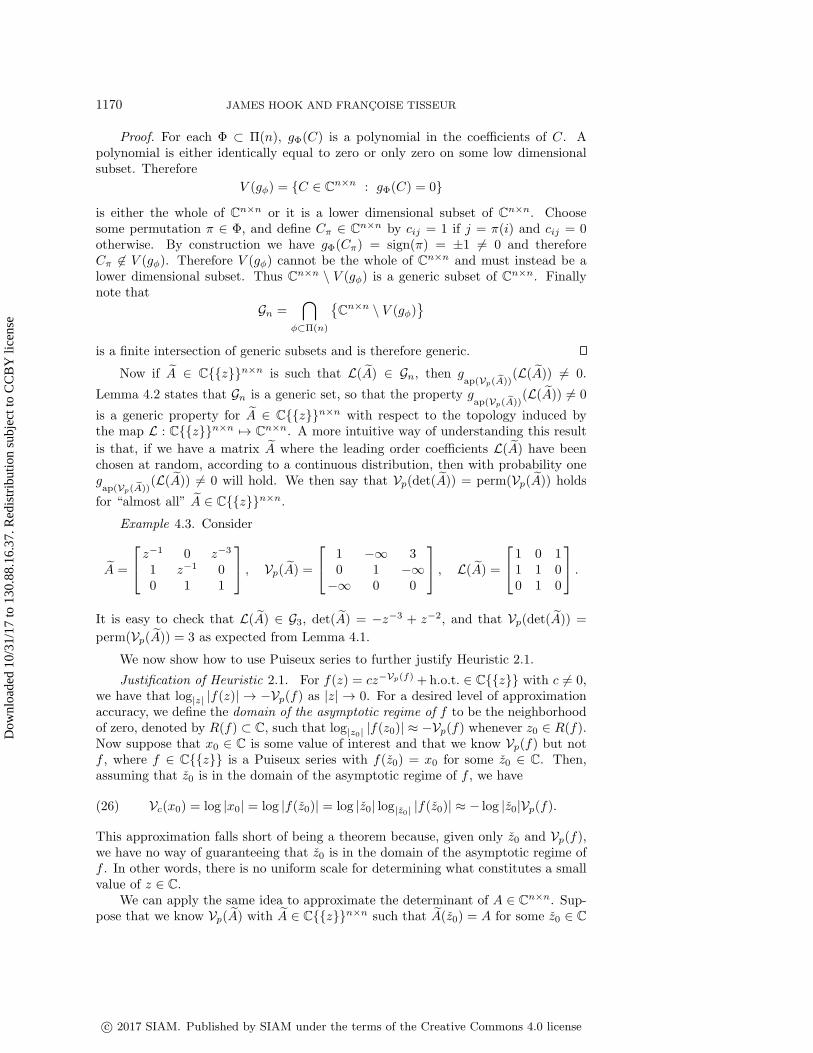
Example 4.3. Consider

A =

z−1 0 z−3

1 z−1 00 1 1

, Vp(A) =

1 −∞ 30 1 −∞−∞ 0 0

, L(A) =

1 0 11 1 00 1 0

.It is easy to check that L(A) ∈ G3, det(A) = −z−3 + z−2, and that Vp(det(A)) =perm(Vp(A)) = 3 as expected from Lemma 4.1.

We now show how to use Puiseux series to further justify Heuristic 2.1.

Justification of Heuristic 2.1. For f(z) = cz−Vp(f) + h.o.t. ∈ C{{z}} with c 6= 0,we have that log|z| |f(z)| → −Vp(f) as |z| → 0. For a desired level of approximationaccuracy, we define the domain of the asymptotic regime of f to be the neighborhoodof zero, denoted by R(f) ⊂ C, such that log|z0| |f(z0)| ≈ −Vp(f) whenever z0 ∈ R(f).Now suppose that x0 ∈ C is some value of interest and that we know Vp(f) but notf , where f ∈ C{{z}} is a Puiseux series with f(z0) = x0 for some z0 ∈ C. Then,assuming that z0 is in the domain of the asymptotic regime of f , we have

(26) Vc(x0) = log |x0| = log |f(z0)| = log |z0| log|z0| |f(z0)| ≈ − log |z0|Vp(f).

This approximation falls short of being a theorem because, given only z0 and Vp(f),we have no way of guaranteeing that z0 is in the domain of the asymptotic regime off . In other words, there is no uniform scale for determining what constitutes a smallvalue of z ∈ C.

We can apply the same idea to approximate the determinant of A ∈ Cn×n. Sup-pose that we know Vp(A) with A ∈ C{{z}}n×n such that A(z0) = A for some z0 ∈ C


Dow

nloa

ded

10/3

1/17

to 1

30.8

8.16

.37.

Red

istr

ibut

ion

subj

ect t

o C

CB

Y li

cens

e


and L(A) ∈ Gn. Then, assuming z0 is in the domain of the asymptotic regime of A,it follows from (26) that

(27) Vc(A) ≈ − log |z0|Vp(A).

Since A(z0) = A we have det(A(z0)) = det(A). Assuming that z0 is in the domain ofthe asymptotic regime of det(A) ∈ C{{z}} and applying (26), we have

Vc(

det(A))≈ − log |z0|Vp(det(A)).

Using Lemma 4.1 and (27), we obtain that Vc(det(A)) ≈ perm(Vc(A)), which providesanother justification for Heuristic 2.1.

We will need the next lemma.

Lemma 4.4. Let C ∈ Cn×n \ Gn with Gn as in (25). Then any k × k submatrixof C is in Ck×k \ Gk.

Proof. If P,Q ∈ Cn×n are permutation matrices, then C ∈ Cn×n \ Gn if and onlyif PCQ ∈ Cn×n \Gn, so it suffices to prove the result for the principal submatrix C oforder k, which we denote by S. For any Ψ ⊂ Π(k) we construct Φ ⊂ Π(n) by settingΦ = {π[ϕ] ∈ Π(n) : ϕ ∈ Ψ}, where

π[ϕ](i) ={ϕ(i), 1 ≤ i ≤ k,i, k + 1 ≤ i ≤ n.

Then

gΦ(C) =∑π∈Φ

sign(π)n∏i=1

ciπ(i) =∑$∈Ψ

sign($)k∏i=1

si$(i)

n∏i=k+1

cii = gΨ(S)n∏

i=k+1

cii

so that gΨ(S) = 0 if and only if gΦ(C) = 0. Hence C ∈ Cn×n \ Gn if and only ifS ∈ Ck×k \ Gk.

As for complex matrices, an LU factorization of A ∈ C{{z}}n×n is a factorizationof A into a lower triangular matrix L ∈ C{{z}}n×n with ones on the diagonal and anupper triangular matrix U ∈ C{{z}}n×n such that A = LU . When the factorizationexists, the nonzero entries of L and U can be defined as in (5)–(6) with A in place ofA. The next result should be compared to Heuristic 3.1.

Theorem 4.5. Let A ∈ C{{z}}n×n be such that L(A) ∈ Gn, and suppose thatVp(A) ∈ Rn×n admits max-plus LU factors L,U ∈ Rn×n. Then A admits an LUfactorization A = LU , where

Vp(L) = L, Vp(U) = U .

If for A ∈ C{{z}}n×n, Vp(A) does not admit max-plus LU factors, then A does notadmit an LU factorization.

Proof. Let A = Vp(A). From Lemmas 4.1 and 4.4 we have

Vp(

det(A([i1, . . . , ik], [j1, . . . , jk])

))= perm

(A([i1, . . . , ik], [j1, . . . , jk])

)for all submatrices of A since L(A) ∈ Gn. Therefore a submatrix of A has zerodeterminant if and only if the corresponding submatrix of Vp(A) has permanent equal


Dow

nloa

ded

10/3

1/17

to 1

30.8

8.16

.37.

Red

istr

ibut

ion

subj

ect t

o C

CB

Y li

cens

e


to minus infinity. Thus if A admits max-plus LU factors, then an LU factorization ofA exists with entries given by (5)–(6).

If Vp(A) does not have max-plus LU factors, then this means that for some i, j, kthe first term on the right-hand side of (7) or (8) is equal to −∞ but the second termis not. As a result, the denominator on the right-hand side of (5) or (6) is equal to 0but the numerator is not, so A does not have an LU factorization.

Recall from section 3 that for A,B, C ∈ Rn×n the product A⊗B balances C if forevery i, j = 1, . . . , n either (A⊗B)ij = cij or (A⊗B)ij = max1≤k≤n(aik + bkj) > cij ,where the maximum must be attained by at least two different values of k.

Lemma 4.6. Let A, B ∈ C{{z}}n×n. Then the product Vp(A) ⊗ Vp(B) balancesVp(AB).

Proof. We have (AB)ij = cz−max1≤k≤n(Vp(aik)+Vp(bkj)) +h.o.t., where c ∈ C is thecoefficient of the lowest order term in the sum. Therefore

(28) Vp(AB)ij = max1≤k≤n

(Vp(aik) + Vp(bkj)) =(Vp(A)⊗ Vp(B)

)ij,

unless c = 0, which is only possible if the maximum in (28) is attained more thanonce, in which case Vp(AB)ij < max1≤k≤n(Vp(aik) +Vp(bkj)) = (Vp(A)⊗Vp(B))ij .

We are now ready to prove Theorems 3.4 and 3.6.

Proof of Theorem 3.4. Suppose that A = Vp(A) ∈ Rn×n admits max-plus LUfactors L,U ∈ Rn×n, where A ∈ C{{z}}n×n is such that L(A) ∈ Gn. Then byTheorem 4.5, A has LU factorization A = LU with Vp(L) = L and Vp(U) = U , andby Lemma 4.6 the product L ⊗ U balances A = Vp(A).

Proof of Theorem 3.6. Let A ∈ C{{z}}n×n satisfy the conditions in the statementof Theorem 4.5. Now let U (k) = Mk · · · M1A = MkU

(k−1) be the matrix obtainedafter k steps of Gaussian elimination applied to A = U (0), where Mk = I−mke

Tk , with

ek the kth unit vector, mk = [0, . . . , 0, mk+1,k, . . . , mn,k]T , and mik = u(k−1)ik /u

(k−1)kk .

By Lemma 4.6, the product Vp(Mk)⊗ Vp(U (k−1)) balances Vp(U (k)), which yields

(29) Vp(u(k)ij ) =: u(k)

ij ≤ max{u(k−1)ij , u(k−1)

ik + u(k−1)kj − u(k−1)

kk }, i, j ≥ k.

Next, we show by induction on k that u(k)ij ≤ maxp,q ap,q for all i, j, and k. Since

U (0) = A, Vp(U (0)) = Vp(A) so that u(0)ij ≤ maxp,q ap,q for all i, j. Assume that

u(`)ij ≤ maxp,q ap,q for all i, j and ` ≤ k − 1. Since A = Vp(A) is partial pivoting free,

u(k−1)kk ≥ u(k−1)

ik , which combined with (29) and the induction hypothesis gives

u(k)ij ≤ max{u(k−1)

ij , u(k−1)kj } ≤ max

p,qap,q

for all i, j. Hence %n(A) = max0≤k≤n−1(maxk≤i,j≤n u(k)ij )−max1≤i,j≤n aij ≤ 0. But,

by definition, %n(A) ≥ 0, so %n(A) = 0.

5. Max-plus LU algorithm. Computing the max-plus LU factors directly fromthe formulae (7)–(8) is computationally expensive, as each entry in either the lowerpart of L or the upper part of U requires the computation of two max-plus permanentsor, in other words, the solution of two optimal assignment problems. The best known


Dow

nloa

ded

10/3

1/17

to 1

30.8

8.16

.37.

Red

istr

ibut

ion

subj

ect t

o C

CB

Y li

cens

e


A =

a b −∞c d e−∞ f −∞

x(1)

x(2)

x(3)

y(1)

y(2)

y(3)

ab

c

de

f

(a)

x(1)

x(2)

x(3)

y(1)

y(2)

y(3)

a−b−c

de

f

(b)

x(1)

x(2)

x(3)

y(1)

y(2)

y(3)

a−b

−cd

e

f

(c)

Fig. 1. (a) Bipartite graph G of A with matching M = {e12, e21} highlighted with thickerlines. (b) Residual graph RG(M) with directed path σ = {e32, e12, e11, e21, e23} highlighted withthicker lines. (c) Transpose residual graph RTG(M) with cycle c = {e12, e22, e21, e11} highlightedwith thicker lines.

algorithms for computing an optimal assignment of A ∈ Rn×nmax have worst case costO(nτ +n2 log n

), where τ is the number of nonzeros in A. So the computation of the

LU factors using (7)–(8) can cost as much as O(n2τ + n3 log n

)operations. We now

describe a more efficient approach, which consists of simultaneously computing all thepermanents needed for all the entries in a row of U or a column of L, while sharingsome of the computation along the way. The bipartite graph setup underpinning ourmethod will be familiar to readers who already have some knowledge of primal dualoptimal assignment solvers such as the Hungarian algorithm.

To A = (aij) ∈ Rn×n we associate a bipartite graph G = (X,Y ;E) with leftvertices X = {x(1), . . . , x(n)}, right vertices Y = {y(1), . . . , y(n)}, and edge set E.We include an edge eij in E from x(i) to y(j) with weight w(eij)) = aij wheneveraij 6= −∞. Thus the edges out of a left vertex x(i) represent the finite entries in theith row of A (see Figure 1(a)).

A matching M is a subset of E with the property that no vertex in M is incidentto more than one edge. Vertices which are incident to edges in M are said to bematched. The weight of a matching w(M) is the sum of its edge weights. Given amatching M , we define the residual graph RG(M) to be the bipartite graph obtainedfrom G by reversing the direction of all of the edges in M and changing the sign ofthe edges’ weights (see Figure 1(b)). Note that we maintain the labelling of edgeseven when they are reversed. Thus eij labels either the forward edge from x(i) toy(j) or the backward edge from y(j) to x(i), depending on whether or not it has beenreversed. We do not switch to labelling this edge as eji. We define the weight w(σ)of a directed path or cycle σ through RG(M) to be equal to the sum of the weightsof its constitute edges in RG(M). For the directed path σ = {e32, e12, e11, e21, e23}through RG(M) in Figure 1(b), w(σ) = f − b+ a− c+ e. We denote by RTG(M) thetranspose residual graph obtained from RG(M) by reversing the direction of all edges(see Figure 1(c)).

Given a subset S of the edges of RG(M), we augment M according to S, written


Dow

nloa

ded

10/3

1/17

to 1

30.8

8.16

.37.

Red

istr

ibut

ion

subj

ect t

o C

CB

Y li

cens

e


as M4S, by taking all the edges that appear in either M or S but not both; that is,

M4S := {M ∪ S} \ {M ∩ S}.

When we augment with respect to a path/cycle through RG(M), we treat the path/cycle as a set of edges. For the path σ = {e32, e12, e11, e21, e23} in Figure 1(b),we have that M4σ = {e11, e23, e32}, which is a matching between the left vertices{x(1), x(2), x(3)} and the right vertices {y(1), y(2), y(3)} with weight w(M4σ) =a+ e+ f = w(M) + w(σ).

Our max-plus LU algorithm relies on the following result.

Proposition 5.1. Let A ∈ Rn×n have max-plus LU factors L = (lij) and U =(uij), and for k = 1, . . . , n let U (k) = (u(k)

ij ) be the intermediate upper factors de-fined in (16). Let G be the bipartite graph associated with A with left vertices X ={x(1), . . . , x(n)} and right vertices Y = {y(1), . . . , y(n)}. Then there exists a se-quence of matchings M` between the left vertices {x(1), . . . , x(`)} and right vertices{y(1), . . . , y(`)}, ` = 1, . . . , n, such that with M0 = ∅,

(i) Mk = Mk−14σ, where σ is the maximally weighted path through RG(Mk−1)from x(k) to y(k);

(ii) uki is either the weight of the maximally weighted path through RG(Mk−1)from x(k) to y(i) for i ≥ k, or −∞ if there is no such path;

(iii) likis either the weight of the maximally weighted path through RTG(Mk) fromx(k) to x(i) for i > k, or −∞ if there is no such path;

(iv) u(k−1)ik is either the weight of the maximally weighted path through RG(Mk−1)

from x(i) to y(k) for i ≥ k, or −∞ if there is no such path.

The proof of Proposition 5.1 is technical and is left to Appendix A. Accordingto Proposition 5.1(i), the sequence of maximally weighted matchings M1, . . . ,Mn canbe obtained iteratively starting with M0 = ∅. At step k > 0, Mk−1 is augmentedwith respect to a maximally weighted path through RG(Mk−1) from x(k) to y(k) toform Mk. From Proposition 5.1(ii), the entries in the kth row of U are given by theweights of n − k different maximally weighted paths through RG(Mk−1). Likewise,from Proposition 5.1(iii), the entries in the kth columns of L are given by the weightsof n − k different maximally weighted paths through RTG(Mk). For a given k, theweights of these maximally weighted paths can be obtained by solving two maximallyweighted spanning tree problems rooted at x(k), one through RG(Mk−1), the otherthrough RTG(Mk). A maximally weighted spanning tree T through RG(M) rootedat x(k) consists of the maximally weighted paths from x(k) to every reachable leftand right vertex. The depth of a reachable vertex is the weight of the correspondingmaximally weighted path in T . If T does not reach a vertex, then this vertex hasdepth −∞. All these facts lead to the following algorithm.

Algorithm 5.2 (max-plus LU). Given A ∈ Rn×n, this algorithm returns a unitlower triangular matrix L and an upper triangular matrix U such that L,U are max-plus LU factors for A.

% G denotes the bipartite graph associated with A with left vertices% X = {x(1), . . . , x(n)} and right vertices Y = {y(1), . . . , y(n)}.

1 Set the lower part of U and strictly upper part of L to −∞, and the diagonalentries of L to 0.

2 Set M0 = ∅.3 for k = 1 : n4 Compute the maximally weighted spanning tree T through RG(Mk−1)


Dow

nloa

ded

10/3

1/17

to 1

30.8

8.16

.37.

Red

istr

ibut

ion

subj

ect t

o C

CB

Y li

cens

e


rooted at x(k).5 for j = k : n6 ukj = depth of y(j) in T .7 end8 Mk = Mk−14σ, where σ is the maximally weighted path through

RG(Mk−1) from x(k) to y(k).9 Compute the maximally weighted spanning tree T ′ through RTG(Mk)

rooted at x(k).10 for i = k + 1 : n11 lik = depth of x(k) in T ′.12 end13 end

If A does not admit max-plus LU factors, then at some step k of Algorithm 5.2,y(k) will have depth −∞ and there will be no path from x(k) to y(k), so the algorithmwill not be able to augment the matching Mk−1 in line 8.

x(1)

x(2)

x(3)

y(1)

y(2)

y(3)

13 0

1

0

0

(a) RG(M0) = G.

x(1)

x(2)

x(3)

y(1)

y(2)

y(3)

−1

3 0

1

0

0

(b) RG(M1).

x(1)

x(2)

x(3)

y(1)

y(2)

y(3)

−1

30

−1

00

(c) RG(M2).

x(1)

x(2)

x(3)

y(1)

y(2)

y(3)

−1

3 0

1 0

0

(d) RTG(M1).

x(1)

x(2)

x(3)

y(1)

y(2)

y(3)

−1

3 0−1

0

0

(e) RTG(M2).

Fig. 2. Bipartite graphs produced by Algorithm 5.2 for the matrix A of Example 5.3. Maximallyweighted spanning trees and paths are highlighted in thicker red lines.

Example 5.3. We apply Algorithm 5.2 to compute the max-plus LU factors for

A =

1 −∞ 30 1 −∞−∞ 0 0

.k = 1. The maximally weighted spanning tree T through RG(M0) = G rooted at

x(1) is highlighted with thicker red lines in Figure 2(a). The depths of theY vertices (i.e., 1 for y(1), −∞ for y(2), as it is not reached by the spanningtree, and 3 for y(3)) give the entries for the first row of U .The maximally weighted path σ through RG(M0) from x(1) to y(1) consistsof a single edge σ = {e11} so that M1 = M04σ = {e11}, yielding the residualgraph RG(M1) displayed in Figure 2(b).


Dow

nloa

ded

10/3

1/17

to 1

30.8

8.16

.37.

Red

istr

ibut

ion

subj

ect t

o C

CB

Y li

cens

e


The maximally weighted spanning tree T ′ through RTG(M1) rooted at x(1) ishighlighted with thicker red lines in Figure 2(d). The depths of the X verticesgive the entries for the first column of L.

k = 2. Figure 2(b) highlights the maximally weighted spanning tree T through theresidual graph RG(M(1)) rooted at x(2). The depths of the Y vertices givethe entries for the second row of U .The maximally weighted path σ through RG(M1) from x(2) to y(2) consists ofa single edge σ = {e22} (Figure 2(b)) so that M(2) = M(1)4σ = {e11, e22}.The residual graph RG(M(2)) is shown in Figure 2(c). The maximallyweighted spanning tree T ′ through RTG(M(2)) rooted at x(2) is highlightedin Figure 2(e). The depths of the X vertices give the entries for the secondcolumn of L below the diagonal.

k = 3. The maximally weighted spanning tree T through RG(M2) rooted at x(3) ishighlighted in Figure 2(c). The depth of the y(3) vertex gives the entry forthe third row of U .

The algorithm returns the max-plus LU factors

L =

0 −∞ −∞−1 0 −∞−∞ −1 0

, U =

1 −∞ 3−∞ 1 2−∞ −∞ 1

.Algorithm 5.2 requires the solution of maximally weighted spanning tree problems

in steps 4 and 9. Note that the spanning tree T in step 4 provides the maximallyweighted path σ needed in step 8. To efficiently solve the maximally weighted spanningtree problems for a given bipartite graph G = (X,Y ;E), we follow an approach takenby Orlin and Lee for the optimal assignment problem [16]. Their approach consistsof adjusting the edge weights of G by defining a potential φ : X,Y 7→ R so that,for each edge e ∈ E from a vertex a to a vertex b, the new edge weight is given byw′(e) = w(e)− φ(a) + φ(b) with the property that w′(e) ≤ 0. This leads to adjustedpath weights w′(σ) = w(σ)−φ(a)+φ(b) for a path σ from vertex a to vertex b. Henceif σ is a maximally weighted path from a to b for the original bipartite graph, thenit stays maximally weighted for the bipartite graph with adjusted weights, and viceversa. Now since all the adjusted edge weights are nonpositive, Dijkstra’s algorithmcan then be used to compute the maximally weighted spanning trees and the depthw′(σ) of each of its maximally weighted paths σ. Then the depth of σ for the originalgraph G is given by w(σ) = w′(σ) + φ(a)− φ(b).

The computational cost of adjusting the weights using the technique in [16] isO(τ) operations, where τ is the number of edges in G. Dijkstra’s algorithm solves themaximally weighted spanning tree problem with worst case cost O

(τ + n log n

)for a

graph with n vertices and τ edges. Since we need to compute 2n of such spanningtrees, our max-plus LU algorithm applied to A ∈ Rn×n will have worst case costO(nτ + n2 log n), where τ is the number of finite entries in A.

5.1. Max-plus LU algorithm for Hungarian matrices. Algorithm 5.2 sim-plifies if we first apply a Hungarian scaling and an optimal assignment to A to producea Hungarian scaled and reordered max-plus matrix H. In particular, if A = Vc(A)with A ∈ Cn×n, then H = Vc(H) with H as in (18) is Hungarian. The next lemmashows that there is no need to compute the sequence of maximally weighted match-ings M1, . . . ,Mn (see step 8 of Algorithm 5.2), as these come for free for Hungarianmatrices.


Dow

nloa

ded

10/3

1/17

to 1

30.8

8.16

.37.

Red

istr

ibut

ion

subj

ect t

o C

CB

Y li

cens

e


Lemma 5.4. Let H ∈ Rn×n be a Hungarian matrix (i.e., hij ≤ 0, hii = 0, 1 ≤i, j ≤ n), and let G = (X,Y ;E) be the corresponding bipartite graph. Then thesets of edges Mk = {e11, . . . , ekk}, k = 1, . . . , n, are maximally weighted matchingsbetween the left vertices {x(1), . . . , x(k)} and the right vertices {y(1), . . . , y(k)} fork = 1, . . . , n.

Proof. We note that every principal submatrix Hk of order k of a Hungarianmatrix H is Hungarian. Since Hk has nonpositive entries,

∑ki=1 hi,π(i) ≤ 0 for any

π ∈ Π(k). Now for π = id, the identity permutation,∑ki=1 hii = 0 so that π = id is an

optimal assignment for Hk. But an optimal assignment corresponds to a permutationrepresenting a maximally weighted perfect matching between the left and right verticesof the bipartite graph associated with Hk; in other words, Mk = {e11, . . . , ekk} is amaximally weighted matching between {x(1), . . . , x(k)} and {y(1), . . . , y(k)}.

Knowing this sequence of maximally weighted matchings a priori enables us toparallelize Algorithm 5.2. We no longer need to compute the maximally weightedpaths throughRG(Mk) before we can formMk+1 and compute the maximally weightedpaths through RG(Mk+1). Instead we can treat each RG(Mk) separately, computingthe kth row of U and (k − 1)th column of L in parallel. This approach yields thefollowing algorithm.

Algorithm 5.5 (max-plus LU for a Hungarian matrix). Given a Hungarian ma-trix H ∈ Rn×n, this algorithm returns a unit lower triangular matrix L and an uppertriangular matrix U such that L,U are max-plus LU factors for H.

% G denotes the bipartite graph associated with H with left vertices% X = {x(1), . . . , x(n)} and right vertices Y = {y(1), . . . , y(n)}.


2 Set M0 = ∅.3 for k = 1 : n4 Set Mk = {e11, . . . , ekk}.5 Compute the maximally weighted spanning tree T through RG(Mk−1)

rooted at x(k).6 for j = k : n7 ukj = depth of y(j) in T .8 end9 Compute the maximally weighted spanning tree T ′ through RTG(Mk)

rooted at x(k).10 for i = k + 1 : n11 lik = depth of x(k) in T ′.12 end13 end

Because the entries of H are nonpositive, we can use Dijkstra’s algorithm tocompute the maximally weighted spanning trees in steps 5 and 9. Thus our max-plusLU algorithm applied to H ∈ Rn×nmax will have worse case cost O

(nτ +n2 log n

), where

τ is the number of finite entries in H.Dijkstra’s algorithm permanently labels vertices in decreasing order of their depth

in the tree. This means that when we run Dijkstra’s algorithm to compute the kthrow of U or kth column of L, we are given the position and value of the entries one ata time in decreasing order of their value. If we are only interested in entries that aregreater than some threshold, or if we only want to know the m largest entries in each


Dow

nloa

ded

10/3

1/17

to 1

30.8

8.16

.37.

Red

istr

ibut

ion

subj

ect t

o C

CB

Y li

cens

e


row, then we can stop Dijkstra’s algorithm earlier and reduce the cost considerably.The exact cost of this implementation will depend heavily on the particular details ofthe problem matrix. This approach will not work for a non-Hungarian scaled matrixas, while Dijkstra’s algorithm will always label vertices in decreasing order, it will bein the order of their adjusted depths. So we cannot be sure that we have found the mlargest entries until we have computed all of the adjusted depths and then convertedthem back into their true depths using the potential.

5.2. Max-plus LU algorithm with partial pivoting. At each step k of Al-gorithm 5.6, the unmatched left vertices are permuted to maximize the weight of theaugmenting path. For this we find a maximally weighted path through RG(Mk−1)from {x(k), . . . , x(n)} to y(k). If this maximally weighted path begins at x(i), thenwe interchange x(i) with x(k) and perform step k of Algorithm 5.2. This is analogousto interchanging rows in Gaussian elimination with partial pivoting. Note that wecan compute the maximally weighted path through RG(Mk−1) from {x(k), . . . , x(n)}to y(k) by solving a single maximally weighted spanning tree problem. This is doneby adding a root vertex r and connecting it to each unmatched left vertex x(j),j = k, . . . , n, with an edge of weight zero (see Figure 3(a)). We then compute the max-imally weighted spanning tree through RG(Mk−1)∪{r} rooted at r. Then, rather thanchoosing the starting vertex of the maximally weighted path from {x(k), . . . , x(n)} toy(k), we take the second vertex on the maximally weighted path from r to y(k). Thisensures the same choice of vertex, but the algorithm requires us to compute fewermaximally weighted spanning trees. This approach yields the following algorithm.

Algorithm 5.6 (max-plus LU with partial pivoting). Given A ∈ Rn×n, thisalgorithm returns a permutation π, a unit lower triangular matrix L, and an uppertriangular matrix U such that L,U are max-plus LU factors for the partial pivotingfree matrix Pπ ⊗A, where (Pπ)ij = 0 for j = π(i) and (Pπ)ij = −∞ otherwise.

% Gπ denotes the bipartite graph associated with A with left vertices% Xπ = {x(π(1)), . . . , x(π(n))} and right vertices Y = {y(1), . . . , y(n)}% for some permutation π.


2 Set M0 = ∅ and π = [1, 2, . . . , n].3 for k = 1 : n4 Add a root vertex r and connect it to each left vertex x

(π(j)

),

j = k, . . . , n, by an edge of weight zero.5 Compute the maximally weighted spanning tree T through RGπ (Mk−1)

rooted at r.6 Swap π(k) with π(i), where x(π(i)) is the 2nd vertex on the maximally

weighted path from r to y(k).7 for j = k, . . . , n8 ukj = depth of y(j) in T.9 end

10 Mk = Mk−14σ, where σ is the maximally weighted path throughRGπ (Mk−1) from x(π(k)) to y(k).

11 Compute the maximally weighted spanning tree T ′ through RTGπ (Mk)rooted at x(π(k)).

12 for i = k + 1 : n13 lik = depth of x(π(k)) in T ′.14 end15 end


Dow

nloa

ded

10/3

1/17

to 1

30.8

8.16

.37.

Red

istr

ibut

ion

subj

ect t

o C

CB

Y li

cens

e


Line 6 in Algorithm 5.6 is the row interchanging step. Since we added a rootvertex r before the left vertices Xπ = {x(π(1)), . . . , x(π(n))}, we need to look for thesecond vertex, say x(π(i)), on the maximally weighted path from r to y(k), the firstvertex being r. We then swap π(k) with π(i), which corresponds to interchangingx(π(k)) with x(π(i)).

Proposition 5.7. For A ∈ Rn×n, Algorithm 5.6 returns a permutation π suchthat the permuted matrix Pπ ⊗A is partial pivoting free.

Proof. Applying the result of Proposition 5.1(iv) to the matrix Pπ ⊗A, we havethat u(k)

i,k+1 is the weight of the maximally weighted path through RG(Mk) from x(i)to y(k+ 1) for i ≥ k+ 1. But from line 6 in Algorithm 5.6 we are guaranteed becauseof the interchanging that the maximally weighted path from {x(k + 1), . . . , x(n)} toy(k + 1) is the path from x(k + 1) to y(k + 1) so that u(k)

k+1,k+1 = maxk+1≤i≤n u(k)i,k+1,

k = 0, . . . , n − 1, which is the definition of max-plus partial pivoting free as given in(15).

x(1)

x(2)

r

y(1)

y(2)

0

0

1

2

3

5

(a) RGπ (M0) ∪ {r}.

x(2)

x(1)

y(1)

y(2)

−3

5

1

2

(b) RGπ (M1).

x(2)

x(1)

y(1)

y(2)

−3

51

2

(c) RTGπ (M1).

x(2)

x(1)

r

y(1)

y(2)

0

−3

5

1

2

(d) RGπ (M1) ∩ {r}.

Fig. 3. Bipartite graphs produced by Algorithm 5.6 applied to A =[ 13

25

].

Example 5.8. Let us apply Algorithm 5.6 to A =[ 1

325

]. Let π = [1, 2].

k = 1. We adjoin a root vertex r to the bipartite graph RGπ (M0) = Gπ and connectit to the left vertices of x(π(1)), x(π(2)) by an edge of weight zero. Themaximally weighted spanning tree T through RGπ (M0) ∪ {r} rooted at r isshown with thicker lines in Figure 3(a). The depths of the Y vertices (i.e., 3 fory(1) and 5 for y(2)) define the entries of the first row of U . Since the maximallyweighted path is the one from x(π(2)), we swap π(1) with π(2) so that π =[2 1]. Then the maximally weighted path σ through RGπ (M0) from x(π(1))to y(1) consists of a single edge {eπ(1),1} = {e21}, so that M1 = M04{e21} ={e21}, yielding the residual graph RGπ (M1) displayed in Figure 3(b). Themaximally weighted spanning tree T ′ through RTGπ (M1) rooted at x(π(1)) =x(2) is highlighted with thicker red lines in Figure 3(c). The depths of thepath from x(π(1)) to x(π(2)), i.e., −2, defines l21.

k = 2. We adjoin a root vertex r to the bipartite graph RGπ (M1). Figure 3(d) high-lights the maximally weighted spanning tree T through RGπ (M1)∪{r} rootedat r. The depths of the Y vertices define the last row of U .


Dow

nloa

ded

10/3

1/17

to 1

30.8

8.16

.37.

Red

istr

ibut

ion

subj

ect t

o C

CB

Y li

cens

e


Hence we obtain

Pπ⊗A =[−∞ 0

0 −∞

]⊗[

1 23 5

]=[

3 51 2

], L =

[0 −∞−2 0

], U =

[3 5−∞ 3

].

5.3. Max-plus ILU preconditioner. Given the max-plus LU factors L and Uof Vc(A), we define the max-plus ILU preconditioner as follows. For a threshold t westore

(30) Sij ={

1 if lij ≥ log t+ maxk log |aik| or uij ≥ log t+ maxk log |aik|,0 otherwise.

We then compute the ILU factors for A restricted to positions where S is nonzerousing, for example, the general static pattern ILU algorithm described in [17, Alg. 10.1]or the more practical variant [17, Alg. 10.3].

6. Numerical experiments. For our numerical experiments, we select all realnonsymmetric matrices in the University of Florida sparse matrix collection [4] of size100 ≤ n ≤ 5000 that have numeric value symmetry no greater than 0.9, and that arestructurally nonsingular. When two matrices from the same group have size n andnumber of nonzero entries within 1% of each other, then we consider these matrices asduplicate and remove one of them. This leaves us with a total of 260 matrices. We usedMATLAB version R2015b to perform the computations. Note that our max-plus LUalgorithms are implemented as research codes rather than efficient implementationsand, for this reason, we only work with matrices of moderate sizes. For the valuationVc we use the logarithm to base 10.

6.1. Stability of Gaussian elimination with no pivoting. The aim of ourfirst set of experiments is to compare the numerical stability of Gaussian eliminationwith no pivoting applied to Hungarian scaled and reordered matrices H in (18), andto reordered matrices PπA, where π is the permutation returned by Algorithm 5.6.For each matrix A in the test set we construct H using the HSL code MC64 [18] andPπA using our MATLAB implementation of Algorithm 5.6. Theorem 3.6 togetherwith Heuristic 3.7 suggests that the growth factors for both H and PπA are of orderone since both Vc(H) and Vc(PπA) are partial pivoting free. Although this is justa heuristic, we expect the LU factorization with no pivoting of H and PπA to havebetter numerical stability than for A. To examine the stability of Gaussian eliminationon these two classes of matrices we compute the relative backward errors

ηX =‖X − LU‖F‖X‖F

for X = H and X = PπA, where L and U are the computed LU factors of the LUfactorization of X. We also use Gaussian elimination with no pivoting to computethe LU factorizations of the original matrices A. For each class of matrices, i.e.,X = A,H and PπA, we plot in Figure 4 the proportion of problems for which weare able to compute LU factors without breakdown and with ηX ≤ α against α. Ifthe factorization breaks down or if ηX ≥ 10−1, we record a fail. Without pivoting orscaling, the LU factorization fails for almost half of the test matrices A, and ηA ≤10−10 for 53% of the test matrices. After applying the max-plus LU permutation Pπto A, the number of failed LU factorizations falls from 120 to 60, and ηPπA ≤ 10−10

for 64% of the test matrices. The number of failed LU factorizations is lower forHungarian scaled matrices H (only 23 fails), and ηH ≤ 10−10 for 86% of the testmatrices. Since our aim is to build a new class of ILU preconditioners and because


Dow

nloa

ded

10/3

1/17

to 1

30.8

8.16

.37.

Red

istr

ibut

ion

subj

ect t

o C

CB

Y li

cens

e


10-15

10-10

10-5

α

0

0.2

0.4

0.6

0.8

1

ProportionofproblemswithηX≤

α

X = A (120 fails)

X = Pπ A (60 fails)

X = H (23 fails)

Fig. 4. Proportion of problems with relative backward error ηX ≤ α for X = A,H, PπA.

• for the vast majority of matrices in the test set a reasonably stable LU fac-torization with no pivoting is possible if A is Hungarian scaled and reorderedinto H,

• Hungarian scaling has been shown experimentally to be beneficial for iterativemethods [2],

• the max-plus LU algorithm is easier to implement for Hungarian scaled ma-trices,

from here on we will work with the subset of test problems for which the Hungarianscaled and reordered matrix H can be factorized with no pivoting and with ηH < 0.1.This results in a test subset of 233 matrices.

6.2. Max-plus LU approximation. The max-plus LU approximation can as-sist in the computation of an ILU preconditioner by providing a prediction of thepositions of larger entries in the LU factors of H. One way of measuring the qualityof this prediction is to treat the max-plus LU approximation as a binary classifier.For the LU factorization H = LU of a matrix H from the test set and its max-plusLU factors L,U , we predict that |lij | ≥ 10−t for i > j if and only if lij ≥ −t, andlikewise for the entries of U . The entries of L and U are then labeled as true positiveor true negative according to the scheme displayed in Figure 5(a). (For example, fora given t, the (i, j) entry of L is true positive if lij ≥ −t and log10 |lij | ≥ −t.) Theaccuracy of the classifier is defined by

accuracy =number of true positives and true negatives

number of nonzeros in L and U,

and the precision is defined by

precision =number of true positives

number of entries in L and U such that |lij | ≥ 10−t and |uij | ≥ 10−t.

We also define the soft accuracy and soft precision, which are calculated in the sameway using the number of entries in L and U that are soft true positive and soft truenegative, where the labelling “soft true positive” and “soft true negative” is done


Dow

nloa

ded

10/3

1/17

to 1

30.8

8.16

.37.

Red

istr

ibut

ion

subj

ect t

o C

CB

Y li

cens

e


lij , uij

log10 |lij |, log10 |uij |

false -ve true +ve

false +vetrue -ve

-2

(a)

lij , uij

log10 |lij |, log10 |uij |

softtrue +ve

softtrue -ve

-1

-2

-3

(b)

Fig. 5. Labelling of the nonzero entries in the L and U factors for calculating (soft) accuracyand (soft) precision for t = 2. The axes cross at (−2,−2).

Table 1Proportion of test problems with with (soft) accuracy and (soft) precision greater than p for

t = 2.

p 0.8 0.85 0.9 0.95A(p) 85% 83% 79% 71%SA(p) 97% 93% 90% 85%P (p) 86% 83% 80% 59%SP (p) 93% 91% 89% 72%

according to the scheme displayed in Figure 5(b). We record in Table 1 the followingproportions:

A(p) = proportion of test examples with accuracy ≥ p,SA(p) = proportion of test examples with soft accuracy ≥ p,P (p) = proportion of test examples with precision ≥ p,

SP (p) = proportion of test examples with soft precision ≥ p,

for p = 0.80, 0.85, 0.9, 0.95 and t = 2. The scores in Table 1 are quite high andshow that, for our test set, the max-plus LU factors provide a good prediction of theposition of the larger entries in L and U .

6.3. Behavior of max-plus ILU preconditioning. In this section, we exam-ine the behavior of our max-plus ILU preconditioner on our test set of 233 Hungar-ian matrices H. We apply GMRES with a right ILU preconditioner to the systemsHx = b. For the ILU preconditioner, we use one of the following:

1. Threshold ILU as implemented in the ilu function of MATLAB with the op-tion setup.type = ’crout’, which performs the Crout version of the thresh-old ILU factorization (see [17, sec. 10.4.6]) and drop tolerance equal to 10−2,which means that the nonzero and nondiagonal entries of U and L satisfy

|uij | ≥ 10−2‖H(i, :)‖2, |lij | ≥ 10−2‖H(:, j)‖2/|ujj |.

Since the Hungarian scaled matrices we are working with typically have allrow/col norms O(1), this choice of dropping strategy is roughly equivalent tothe max-plus method we describe below.


Dow

nloa

ded

10/3

1/17

to 1

30.8

8.16

.37.

Red

istr

ibut

ion

subj

ect t

o C

CB

Y li

cens

e


Table 2Number of test matrices N for which ILU(k) is used with level k.

Level k 0 1 2 3 4 5 ≥ 6# of test matrices 104 45 28 10 8 4 34

1 2 3 4 5 6

α

0

0.2

0.4

0.6

0.8

1

within

αof

best

Cost of GMRES solve (maxit = 100, right precond)

threshold ILU (15 fails)max-plus ILU (38 fails)ILU(k) (59 fails)ILU(0) (88 fails)no precond (144 fails)

1 2 3 4 5 6

α

0

0.2

0.4

0.6

0.8

1

within

αof

best

Cost of BICGSTAB solve (maxit = 100)

threshold ILU (42 fails)max-plus ILU (59 fails)ILU(k) (61 fails)ILU(0) (98 fails)no precond (157 fails)

Fig. 6. Performance profile comparing relative costs of GMRES (left plot) and BiCGSTAB(right plot) solves for different ILU preconditioning strategies.

2. ILU(k) through the MATLAB function iluk from [13], which is an optimizedimplementation of the incomplete LU factorization with fill level k describedin [17, Chap. 10].

3. ILU(0) with zero level of fill-in.4. Max-plus ILU by forming the pattern matrix S in (30) with t = 10−2 and by

calling iluk with input parameters set up to bypass the symbolic factoriza-tion.

The level k for ILU(k) is chosen as the smallest integer such that the resulting ILUfactors are denser than those obtained by the max-plus method. We justify this choiceat the end of this section. The distribution of the levels k is shown in Table 2.

We use unrestarted GMRES and stop the iterations when either the approximatesolution x satisfies ‖Hx − b‖2 ≤ 10−5‖b‖2, in which case we say that GMRES hasconverged, or the maximum number of iterations has been reached (maxit=100), inwhich case the test matrix is marked as a fail. For each preconditioned system, werecord the number of GMRES iterations required for convergence multiplied by thesum of the number of nonzero entries in H and the number of nonzero entries in theILU factors. For the unpreconditioned systems we record the number of GMRESiterations multiplied by the number of nonzero entries in H. These measures givean approximation of the cost of the GMRES solves but do not include the cost ofconstructing the preconditioner. The left plot in Figure 6 is a performance profile thatcompares this cost measure over the different ILU strategies. For the unpreconditionedsystems, GMRES fails to converge in less than maxit = 100 iterations for 144 outof 233 problems and has clearly the worse performance. Systems preconditioned byILU(k) have a cost more than double that of the best method for about 50% of theproblems. The figure shows that the performance of the max-plus ILU preconditionedsystems is close to that of the standard threshold ILU preconditioned systems. Forabout 80% of problems the cost of the max-plus method is within a factor of 2 of


Dow

nloa

ded

10/3

1/17

to 1

30.8

8.16

.37.

Red

istr

ibut

ion

subj

ect t

o C

CB

Y li

cens

e


the best method. We obtain an almost identical performance profile plot for GMRESwith left ILU preconditioners.

We performed the same set of tests but with BiCGSTAB in place of GMRESfor the iterative solver. The corresponding performance profile (see Figure 6(right))shows that the different ILU preconditioners exhibit the same behavior as for GMRES.

The cost measure that we have used for these performance profiles tends to de-crease with the number of nonzero positions included in the ILU factors for all threedifferent ILU techniques. As a result, our choice for the level k is slightly generousto the ILU(k) method. Of course the total cost of solving the linear system shouldalso include the cost of computing the ILU factors, which generally increases with thenumber of nonzero positions allowed, so that in practice choosing denser ILU factorsis not always an advantage. We use this cost measure here for its simplicity. In futurework we hope to develop an efficient implementation of our max-plus ILU algorithmthat can be timed against state-of-the-art ILU(k) and threshold ILU methods.

7. Conclusion. We have presented a new method for approximating the orderof magnitude of the entries in the LU factors of a matrix A ∈ Cn×n. This methoduses max-plus algebra and is based solely on the moduli of the entries in A. If thematrix A is first Hungarian scaled and reordered, then this LU approximation can becomputed in parallel with n independent computations, of cost O(τ + log n). If weseek only the positions and values of the largest entries in the LU factors, then thiscost can be reduced further.

We have shown that this approximation can be used to help compute an ILUpreconditioner for A. First we reorder and rescale A to obtain a Hungarian matrixH, then we compute the positions of the largest entries in the LU factors of H, andfinally we use these positions as the sparsity pattern for an ILU preconditioner. Theresulting preconditioner tends to outperform the comparable ILU(k) preconditionerand have performance very close to a comparable threshold ILU preconditioner whenapplied as preconditioner to GMRES or BiCGSTAB.

Like the traditional threshold ILU method, the idea behind our max-plus pre-conditioner is to try to capture the largest entries in the exact LU factors of A. Byattempting to find the locations of these large entries a priori using our heuristic max-plus approximation, we trade some accuracy for potential computational advantage.Inaccuracy in the approximation results in slightly less effective preconditioners whencompared to the threshold method. But since the columns of the max-plus sparsitypattern can be computed independently of each other and since we can then use thesame techniques as in ILU(k) to compute the numerical factors, there is potential todevelop a scalable parallel algorithm for max-plus ILU preconditioning.

The numerical examples presented in this paper represent a proof of principalthat the max-plus ILU technique can be advantageous in the solution of sparse linearsystems.

Appendix A. This appendix presents several technical results needed to proveProposition 5.1. We refer to section 5 for notation and definitions.

Lemma A.1. Let G be a bipartite graph with left vertices X = {x(1), . . . , x(n)}and right vertices Y = {y(1), . . . , y(n)}, and let M be a matching between {x(1), . . . ,x(k)} and {y(1), . . . , y(k)}. The following statements hold:

(i) If σ is a direct path through the residual graph RG(M) from the unmatchedleft vertex x(k + 1) to the unmatched right vertex y(k + 1), then M4σ isa matching between the left vertices {x(1), . . . , x(k), x(k + 1)} and the right


Dow

nloa

ded

10/3

1/17

to 1

30.8

8.16

.37.

Red

istr

ibut

ion

subj

ect t

o C

CB

Y li

cens

e


vertices {y(1), . . . , y(k), y(k + 1)}, with weight w(M4σ) = w(M) + w(σ).(ii) If C is a cycle through the residual graph RG(M), then M4C is a matching

between the same vertices as M with weight w(M4C) = w(M) + w(C).(iii) If σ is a direct path through the residual graph RG(M) from the unmatched

left vertex x(k+ 1) to the matched left vertex x(k), then M4σ is a matchingbetween the left vertices {x(1), . . . , x(k + 1)} \ {x(k)} and the right vertices{y(1), . . . , y(k)} with weight w(M4σ) = w(M) + w(σ).

(iv) If S1 and S2 are disjoint subsets of edges, each either a path or a cycle inRG(M), then w(M4(S1 ∪ S2)) = w(M) + w(S1) + w(S2).

Proof. (i) There are no edges into any unmatched left vertices or out of anyunmatched right vertices, so that σ can only visit its origin vertex x(k+1), destinationvertex y(k+ 1), as well as the vertices matched by M . Since σ is a path from x(k+ 1)it must include exactly one edge out of this vertex, and since this vertex is unmatchedin M there can be no edge out of it in M . Thus M4σ contains exactly one edgeincident to the origin vertex x(k + 1). Likewise for the destination vertex, M4σcontains exactly one edge incident to y(k + 1).

Let u be a matched left vertex visited by σ. Then σ must include an edge into u,which, being a right-to-left edge, must be an edge in M ; σ must also include an edgeout of u, which, being a left-to-right edge, must not be in M . Thus M4σ containsexactly one edge incident to u. Likewise if v is a matched right vertex visited by σ,then M4σ contains exactly one edge incident to v.

Matched vertices that are not visited by σ are unaffected; likewise unmatchedvertices are unaffected. Thus M4σ is a subset of E, with exactly one edge incidentto each of the left vertices {x(1), . . . , x(k), x(k + 1)} and each of the right vertices{y(1), . . . , y(k), y(k + 1)}, and no edge incident to any other vertices.

The weight of M4σ is equal to w(M) plus the weight of any edges in σ but not inM minus the weight of any edges in M and σ. Since any edge in M ∩σ is a backwardedge with an extra minus sign and any edge in σ/M is a forwards edge without anextra minus sign, we have w(M4σ) = w(M) + w(σ).

(ii) The proof of (ii) is the same as for (i) but without the origin or destinationvertices.

(iii) The argument is the same as (i) except for the destination vertex x(k). Thisvertex is incident to exactly one edge in M , which is a right-to-left vertex; since σ endsat this vertex it must also contain this edge, and therefore M4σ does not contain anedge incident to x(k).

(iv) Since S1 ∪ S2 = ∅ we have M4(S1 ∪ S2) = (M4S1)4S2. Hence,

w((M4S1)4S2

)= w(M4S1) + w(S2),

where w(S2) is the weight of the edge set S2 in the residual graph RG(M4S1).However, since S1 and S2 are disjoint we have w(S2) = w(S2), where w(S2) is theweight of the edge set S2 in the residual graph RG(M). (This follows because noneof the edges affected by augmenting with respect to S1 are in the set S2.) Thereforewe have

w(M4(S1 ∪ S2)

)= w

((M4S1)4S2

)= w(M4S1) + w(S2)= w(M) + w(S1) + w(S2).

For the residual graph RG(M) in Figure 1(b) and


Dow

nloa

ded

10/3

1/17

to 1

30.8

8.16

.37.

Red

istr

ibut

ion

subj

ect t

o C

CB

Y li

cens

e


(i) the path σ = {e32, e12, e11, e21, e23}, we have that M4σ = {e11, e23, e32},which is a matching between the left vertices {x(1), x(2), x(3)} and the rightvertices {y(1), y(2), y(3)} with weight w(M4σ) = a+ e+ f = w(M) +w(σ);

(ii) the cycle c = {e22, e12, e11, e21} through RG(M) with weight w(σ) = d −b + a − c, we have that M4c = {e11, e22}, which is a matching betweenthe left vertices {x(1), x(2)} and the right vertices {y(1), y(2)} with weightw(M4c) = a+ d = w(M) + w(c);

(iii) the path σ = {e32, e12, e11, e21} through RG(M) with weight w(σ) = f −b + a − c, we have that M4σ = {e11, e32}, which is a matching betweenthe left vertices {x(1), x(3)} and the right vertices {y(1), y(2)}, with weightw(M4σ) = a+ f = w(M) + w(σ).

Lemma A.2. Let G be the bipartite graph associated with A ∈ Rn×n with left ver-tices {x(1), . . . , x(n)} and right vertices {y(1), . . . , y(n)}. Then perm(A([i1, . . . , ik],[j1, . . . , jk]) is the weight of the maximally weighted matching between the left vertices{x(i1), . . . , x(ik)} and the right vertices {y(i1), . . . , y(ik)}.

Proof. Any matching M between the left vertices {x(1), . . . , x(k)} and the rightvertices {y(1), . . . , y(k)} can be represented by a unique permutation π ∈ Π(k) sothat Mπ is the matching that matches x(i) to y

(π(i)

). Now consider w(Mπ) =∑k

i=1 ax(i)y(π(i)) so that the weight of the maximally weighted matching is given by

maxπ∈Π(k)

w(Mπ) = maxπ∈Π(k)

k∑i=1

ax(i)y(π(i)) = perm(A([i1, . . . , ik], [j1, . . . , jk])).

Lemma A.3. Let G = (X,Y ;E) be a bipartite graph, and let Mπ ⊂ E, Mω ⊂ Ebe matchings defined by the permutations π ∈ Π(k) and ω ∈ Π(k + 1), respectively.Then there exists a path σ through RG(M) from x(k+1) to y(k+1) as well as disjointcycles C1, . . . , Cm through RG(M) such that Mω = Mπ4(σ ∪ C1 ∪ · · · ∪ Cm).

Proof. We will prove the lemma by constructing the path and cycles as follows.Set σ(1) = x(k + 1), then set

σ(2) = y(ω(k + 1)

), σ(3) =x

(π−1ω(k + 1)

),

σ(4) = y(ωπ−1ω(k + 1)

), σ(5) =x

(π−1ωπ−1ω(k + 1)

), . . . .

There is no right vertex y(j) with π−1(j) = k+ 1 since the domain of π is {1, . . . , k}.Also all subsequent vertices visited by the constructed path can have only one pre-decessor, as π and ω are permutations. Therefore σ cannot contain any cycle andmust terminate since there are only finitely many vertices that it can visit withoutrepetition. The only way that the path can terminate is by reaching a vertex wherethe next step is not well defined, and the only such vertex is y(k+1). The constructedpath therefore terminates at σ(2`) = y(k + 1).

Next we pick any left vertex x matched by Mπ, which is not visited by σ. Weconstruct a new path starting from x with the same rule that we used for constructingσ. Since there are no possible termination points, where π−1 or ω are not defined,this new path must be cyclic. If the constructed cycle is of length 2, then we discountthe cycle but still record the constituent vertices as having been visited. We constructfurther cycles C1, . . . , Cm until all matched vertices have been visited.

By construction each vertex matched by Mπ either has the same matching underMω or is incident to two edges in σ ∪C1 ∪ · · · ∪Cm, one edge from Mπ and one from


Dow

nloa

ded

10/3

1/17

to 1

30.8

8.16

.37.

Red

istr

ibut

ion

subj

ect t

o C

CB

Y li

cens

e


Mω. When we augment by taking the symmetric difference, the edge from Mπ isreplaced by the one from Mω. Likewise the origin and destination vertices are eachincident to an edge which is in Mω but not in Mπ, so these edges are also includedwhen we augment.

The following theorem shows us how we can obtain a sequence of maximallyweighted matchings by augmenting with respect to maximally weighted paths throughthe residual graph. This is the mechanism by which we will compute all of the entriesin the max-plus LU factors.

Theorem A.4. Let G = (X,Y ;E) be a bipartite graph, and let M be a maximallyweighted matching between the left vertices {x(1), . . . , x(k)} and the right vertices{y(1), . . . , y(k)}. The following hold:

(i) If σ is a maximally weighted path through RG(M) from the unmatched leftvertex x(k + 1) to the unmatched right vertex y(k + 1), then M4σ is a max-imally weighted matching between the left vertices {x(1), . . . , x(k + 1)} andthe right vertices {y(1), . . . , y(k + 1)}.

(ii) If σ be a maximally weighted path through RG(M) from the unmatched leftvertex x(k + 1) to the matched left vertex x(k), then M4σ is a maximallyweighted matching between the left vertices {x(1), . . . , x(k− 1), x(k+ 1)} andthe right vertices {y(k), . . . , y(k)}.

Proof. (i) Let σ be a path through RG(M), and let C1, . . . , Cm be disjoint cyclesin RG(M). Then by Lemma A.1(iv), w(M4(σ ∪ C1 ∪ · · · ∪ Cm)) = w(M) + w(σ) +w(C1) + · · · + w(Cm). It follows from Lemma A.1(ii) that if C is single cycle, thenM4C is a matching between the same vertices as M , and since M is the maximallyweighted matching on its matched vertices, w(M4C) = w(M) +w(C) ≤ w(M), andthus w(C) ≤ 0, showing that any cycle in RG(M) must have nonpositive weight.

Now consider maxM ′ w(M ′), where the maximum is taken over all matchingsfrom {x(1), . . . , x(k + 1)} to {y(k), . . . , y(k + 1)}. Lemma A.3 tells us that everymatching M ′ from {x(1), . . . , x(k + 1)} to {y(k), . . . , y(k + 1)} can be written as theaugmentation of the matching M with respect to some path and cycles. Therefore

maxM ′

w(M ′) = w(M) + maxσ,C1,...,Cm

w(σ) + w(C1) + · · ·+ w(Cm),

where the maximum is taken over all paths through RG(M) from x(k+ 1) to y(k+ 1)and disjoint cycles C1, . . . , Cm in RG(M). Since the cycle weights are all nonpositivewe have

maxM ′

w(M ′) ≤ w(M) + maxσ

w(σ),

and since the upper bound is attained by the matching M ′ = M4 arg maxσ w(σ),where arg maxσ w(σ) is a maximally weighted path through RG(M) from x(k+ 1) toy(k + 1), we have

maxM ′

w(M ′) = w(M4 arg max

σw(σ)

).

Hence M4 arg maxσ w(σ) is a maximally weighted matching between the left vertices{x(1), . . . , x(k + 1)} and the right vertices {y(1), . . . , y(k + 1)}.

(ii) This follows from Lemmas A.1 and A.3 in analogy to Theorem A.4.

We are now ready to prove Proposition 5.1.

Proof of Proposition 5.1. Statement (i) is simply Theorem A.4(i).Statement (ii): Let Mk−1 be a maximally weighted matching between the left

vertices {x(1), . . . , x(k − 1)} and the right vertices {y(1), . . . , y(k − 1)}, and let σ


Dow

nloa

ded

10/3

1/17

to 1

30.8

8.16

.37.

Red

istr

ibut

ion

subj

ect t

o C

CB

Y li

cens

e


be a maximally weighted path through RG(Mk−1) from the unmatched left vertexx(k) to the unmatched right vertex y(j) for j ≥ k. Then from Lemma A.2 we haveperm

(A(1 : k − 1, 1 : k − 1)

)= w(Mk−1). From Theorem A.4 we have that Mk−14σ

is the maximally weighted matching between the left vertices {x(1), . . . , x(k)} and theright vertices {y(1), . . . , y(k − 1), y(j)}. Thus from Lemma A.2 we have perm

(A(1 :

k, [1 : k − 1, j]))

= w(Mk−14σ). Finally, using Lemma A.1, we have w(Mk−14σ) =w(Mk−1) + w(σ), and using the expression for ukj for j ≥ k in (7), we have that

ukj = perm(A(1 : k, [1 : k − 1, j])

)− perm

(A(1 : k − 1, 1 : k − 1)

)= w(Mk−1) + w(σ)− w(Mk−1) = w(σ).

Statement (iii): Let Mk be a maximally weighted matching between the left ver-tices {x(1), . . . , x(k)} and the right vertices {y(1), . . . , y(k)}, and let σ be a maximallyweighted path through RG(Mk) from the unmatched left vertex x(i) with i > k tothe matched left vertex x(k). Then from Lemma A.2 we have perm(A(1 : k, 1 : k)) =w(Mk). From Theorem A.4 we have that Mk4σ is the maximally weighted matchingbetween the left vertices {x(1), . . . , x(k − 1), x(i)} and the right vertices {y(1), . . . ,y(k)}. Thus from Lemma A.2 we have perm(A([1 : k − 1, i], 1 : k)) = w(Mk4σ). Fi-nally, using Lemma A.1, we have w(Mk4σ) = w(Mk)+w(σ), and using the expressionfor lik for i > k in (7), we have that

lik=perm(A([1 : k − 1, i], 1 : k)

)− perm

(A(1 : k, 1 : k)

)=w(Mk) + w(σ)− w(Mk) = w(σ).

Statement (iv): From (16) we have

(31) u(k−1)ik = perm

(A([1 : k − 1, i], [1 : k])

)− perm

(A(1 : k − 1, 1: k − 1)

), i ≥ k.

Let Mk−1 be a maximally weighted matching between the left vertices {x(1), . . . ,x(k − 1)} and the right vertices {y(1), . . . , y(k − 1)}, and let σ be a maximallyweighted path through RG(Mk−1) from the unmatched left vertex x(i) with i ≤ k tothe unmatched right vertex y(k). Then from Lemma A.2 we have

perm(A(1 : k − 1, 1 : k − 1)

)= w(Mk−1).

From Theorem A.4 we have that Mk−14σ is the maximally weighted matching be-tween the left vertices {x(1), . . . , x(k − 1), x(i)} and the right vertices {y(1), . . . ,y(k − 1), y(k)}. Thus from Lemma A.2 we have

perm(A([1 : k − 1, i], [1 : k])

)= w(Mk−14σ).

Finally, using Lemma A.1, we have w(Mk−14σ) = w(M) + w(σ), and substitutingback into (31), we have that

u(k−1)ij = perm

(A([1 : k − 1, i], [1 : k])

)− perm

(A(1 : k − 1, 1: k − 1)

)= w(Mk−1) + w(σ)− w(Mk−1) = w(σ).

REFERENCES

[1] M. Akian, S. Gaubert, and A. Marchesini, Tropical bounds for eigenvalues of matrices,Linear Algebra Appl., 446 (2014), pp. 281–303, https://doi.org/10.1016/j.laa.2013.12.021.


Dow

nloa

ded

10/3

1/17

to 1

30.8

8.16

.37.

Red

istr

ibut

ion

subj

ect t

o C

CB

Y li

cens

e

https://doi.org/10.1016/j.laa.2013.12.021


[2] M. Benzi, J. C. Haws, and M. Tuma, Preconditioning highly indefinite and nonsymmet-ric matrices, SIAM J. Sci. Comput., 22 (2000), pp. 1333–1353, https://doi.org/10.1137/S1064827599361308.

[3] D. A. Bini and V. Noferini, Solving polynomial eigenvalue problems by means of the Ehrlich-Aberth method, Linear Algebra Appl., 439 (2013), pp. 1130–1149, https://doi.org/10.1016/j.laa.2013.02.024.

[4] T. A. Davis and Y. Hu, The University of Florida sparse matrix collection, ACM Trans. Math.Software, 38 (2011), 1, https://doi.org/10.1145/2049662.2049663.

[5] F. R. Gantmacher, The Theory of Matrices, Vol. 1, Chelsea, New York, 1959; ISBN 0-8284-0131-4.

[6] S. Gaubert and M. Sharify, Tropical scaling of polynomial matrices, in Positive Systems,Lecture Notes in Control Inform. Sci. 389, Springer-Verlag, Berlin, 2009, pp. 291–303.

[7] S. Hammarling, C. J. Munro, and F. Tisseur, An algorithm for the complete solution ofquadratic eigenvalue problems, ACM Trans. Math. Software, 39 (2013), 18, https://doi.org/10.1145/2450153.2450156.

[8] N. J. Higham, Accuracy and Stability of Numerical Algorithms, 2nd ed., SIAM, Philadelphia,2002, https://doi.org/10.1137/1.9780898718027.

[9] J. Hook, Max-plus singular values, Linear Algebra Appl., 486 (2015), pp. 419–442, https://doi.org/10.1016/0024-3795(95)00455-6.

[10] J. Hook and F. Tisseur, Max-plus eigenvalues and singular values: A useful tool in numericallinear algebra, manuscript, 2016.

[11] A. S. Householder, The Theory of Matrices in Numerical Analysis, Blaisdell, New York,1964; ISBN 0-486-61781-5.

[12] D. Hysom and A. Pothen, A scalable parallel algorithm for incomplete factor precon-ditioning, SIAM J. Sci. Comput., 22 (2001), pp. 2194–2215, https://doi.org/10.1137/S1064827500376193.

[13] K. Miller, ILU(k) Preconditioner, https://uk.mathworks.com/matlabcentral/fileexchange/48320-ilu-k--preconditioner.

[14] V. Noferini, M. Sharify, and F. Tisseur, Tropical roots as approximations to eigenvaluesof matrix polynomials, SIAM J. Matrix Anal. Appl., 36 (2015), pp. 138–157, https://doi.org/10.1137/14096637X.

[15] M. Olschowka and A. Neumaier, A new pivoting strategy for Gaussian elimination, LinearAlgebra Appl., 240 (1996), pp. 131–151, https://doi.org/10.1016/0024-3795(94)00192-8.

[16] J. B. Orlin and Y. Lee, Quickmatch—A Very Fast Algorithm for the Assignment Problem,Working papers 3547-93, Sloan School of Management, Massachusetts Institute of Tech-nology (MIT), Cambridge, MA, 1993.

[17] Y. Saad, Iterative Methods for Sparse Linear Systems, 2nd ed., SIAM, Philadelphia, 2003,https://doi.org/10.1137/1.9780898718003.

[18] Science and Technology Facilities Council, The HSL Mathematical Software Library,Fortran codes for large scale scientific computation, http://www.hsl.rl.ac.uk/.

[19] M. Sharify, Scaling Algorithms and Tropical Methods in Numerical Matrix Analysis: Appli-cation to the Optimal Assignment Problem and to the Accurate Computation of Eigen-values, Ph.D. thesis, Ecole Polytechnique, Palaiseau, France, 2011; available from http://hal.archives-ouvertes.fr/docs/00/64/38/36/PDF/thesis.pdf.

[20] M. Van Barel and F. Tisseur, Polynomial eigenvalue solver based on tropically scaled La-grange linearization, Linear Algebra Appl., 2017, to appear, https://doi.org/10.1016/j.laa.2017.04.025.


Dow

nloa

ded

10/3

1/17

to 1

30.8

8.16

.37.

Red

istr

ibut

ion

subj

ect t

o C

CB

Y li

cens

e

https://doi.org/10.1137/S1064827599361308

https://doi.org/10.1137/S1064827599361308



https://doi.org/10.1145/2049662.2049663

https://doi.org/10.1145/2450153.2450156

https://doi.org/10.1145/2450153.2450156

https://doi.org/10.1137/1.9780898718027

https://doi.org/10.1016/0024-3795(95)00455-6

https://doi.org/10.1016/0024-3795(95)00455-6

https://doi.org/10.1137/S1064827500376193

https://doi.org/10.1137/S1064827500376193

https://uk.mathworks.com/matlabcentral/fileexchange/48320-ilu-k--preconditioner

https://uk.mathworks.com/matlabcentral/fileexchange/48320-ilu-k--preconditioner

https://doi.org/10.1137/14096637X

https://doi.org/10.1137/14096637X

https://doi.org/10.1016/0024-3795(94)00192-8

https://doi.org/10.1137/1.9780898718003

http://www.hsl.rl.ac.uk/

http://hal.archives-ouvertes.fr/docs/00/64/38/36/PDF/thesis.pdf

http://hal.archives-ouvertes.fr/docs/00/64/38/36/PDF/thesis.pdf



Documents

INCOMPLETE LU PRECONDITIONER BASED ON