Inconsistency of uhyper and umat in Abaqus for compressiblehyperelastic materials

Herbert Baaser1 and Robert J. Martin2 and Patrizio Neff3

September 1, 2017

Dedicated to Zedenek Bažant

Abstract

We demonstrate an error in the implementation of the popular commercial Finite-Element-System Abaqusby an explicit and simple example. This error has previously been brought to attention by Bažant et al. who,in a series of papers, pointed out that the umat user interface subroutine returns erroneous results for nonlinearelastic models of highly compressible materials.

In this paper, we compare the uhyper and umat results for quasi-incompressible (rubber-like) as well asfor highly compressible (foam-like) materials, showing the inconsistencies in the compressible case. We alsoimplement a correction suggested by Bažant to demonstrate its capability to re-establish the correct results.

Mathematics Subject Classification: 74B20, 74S05

Key words: Abaqus, finite element methods, hyperelasticity, finite strain, Jaumann rate, compressible ma-terial, Cauchy stress, tangential stiffness

Contents1 Introduction 2

1.1 Stress rates and time integration . . . . . . . . . . . . . . . . . . . . . . . . . . . . . . . . . . . . . 3

2 Three ways of implementing hyperelasticity in Abaqus 42.1 Bažant’s proposed modification of the tangent modulus . . . . . . . . . . . . . . . . . . . . . . . . 5

3 Examples of numerical results for different implementations 53.1 Quasi-incompressible material behaviour . . . . . . . . . . . . . . . . . . . . . . . . . . . . . . . . . 63.2 Compressible material behaviour . . . . . . . . . . . . . . . . . . . . . . . . . . . . . . . . . . . . . 6

4 Conclusion 7

5 References 81Mechanical Engineering, University of Applied Sciences Bingen, Germany, h.baaser@th-bingen.de2Lehrstuhl für Nichtlineare Analysis und Modellierung, Fakultät für Mathematik, Universität Duisburg–Essen, Thea-Leymann

Str. 9, 45127 Essen, Germany, robert.martin@uni-due.de3Head of Lehrstuhl für Nichtlineare Analysis und Modellierung, Fakultät für Mathematik, Universität Duisburg–Essen, Thea-

Leymann Str. 9, 45127 Essen, Germany, patrizio.neff@uni-due.de

1

arX

iv:1

708.

0969

9v1

[m

ath.

NA

] 3

1 A

ug 2

017

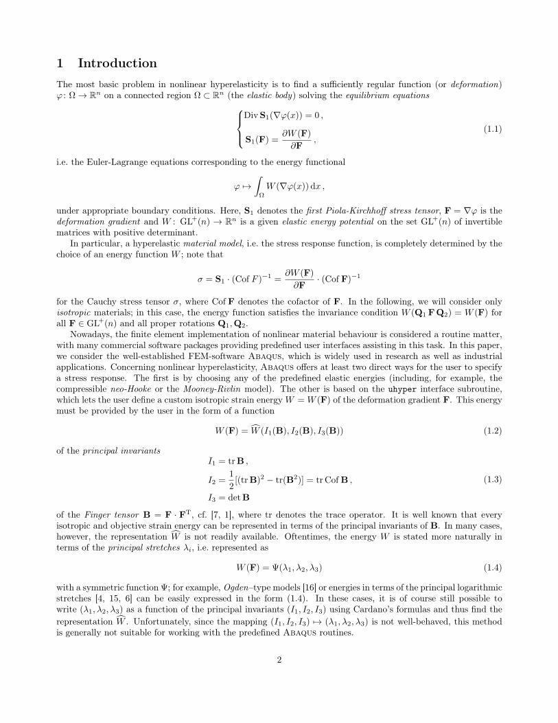
1 IntroductionThe most basic problem in nonlinear hyperelasticity is to find a sufficiently regular function (or deformation)ϕ : Ω→ Rn on a connected region Ω ⊂ Rn (the elastic body) solving the equilibrium equations

DivS1(∇ϕ(x)) = 0 ,

S1(F) =∂W (F)

∂F,

(1.1)

i.e. the Euler-Lagrange equations corresponding to the energy functional

ϕ 7→∫

Ω

W (∇ϕ(x)) dx ,

under appropriate boundary conditions. Here, S1 denotes the first Piola-Kirchhoff stress tensor, F = ∇ϕ is thedeformation gradient and W : GL+(n) → Rn is a given elastic energy potential on the set GL+(n) of invertiblematrices with positive determinant.

In particular, a hyperelastic material model, i.e. the stress response function, is completely determined by thechoice of an energy function W ; note that

σ = S1 · (Cof F )−1 =∂W (F)

∂F· (Cof F)−1

for the Cauchy stress tensor σ, where Cof F denotes the cofactor of F. In the following, we will consider onlyisotropic materials; in this case, the energy function satisfies the invariance condition W (Q1 FQ2) = W (F) forall F ∈ GL+(n) and all proper rotations Q1,Q2.

Nowadays, the finite element implementation of nonlinear material behaviour is considered a routine matter,with many commercial software packages providing predefined user interfaces assisting in this task. In this paper,we consider the well-established FEM-software Abaqus, which is widely used in research as well as industrialapplications. Concerning nonlinear hyperelasticity, Abaqus offers at least two direct ways for the user to specifya stress response. The first is by choosing any of the predefined elastic energies (including, for example, thecompressible neo-Hooke or the Mooney-Rivlin model). The other is based on the uhyper interface subroutine,which lets the user define a custom isotropic strain energyW = W (F) of the deformation gradient F. This energymust be provided by the user in the form of a function

W (F) = W (I1(B), I2(B), I3(B)) (1.2)

of the principal invariantsI1 = trB ,

I2 =1

2[(trB)2 − tr(B2)] = tr Cof B ,

I3 = detB

(1.3)

of the Finger tensor B = F · FT, cf. [7, 1], where tr denotes the trace operator. It is well known that everyisotropic and objective strain energy can be represented in terms of the principal invariants of B. In many cases,however, the representation W is not readily available. Oftentimes, the energy W is stated more naturally interms of the principal stretches λi, i.e. represented as

W (F) = Ψ(λ1, λ2, λ3) (1.4)

with a symmetric function Ψ; for example, Ogden–type models [16] or energies in terms of the principal logarithmicstretches [4, 15, 6] can be easily expressed in the form (1.4). In these cases, it is of course still possible towrite (λ1, λ2, λ3) as a function of the principal invariants (I1, I2, I3) using Cardano’s formulas and thus find therepresentation W . Unfortunately, since the mapping (I1, I2, I3) 7→ (λ1, λ2, λ3) is not well-behaved, this methodis generally not suitable for working with the predefined Abaqus routines.

2

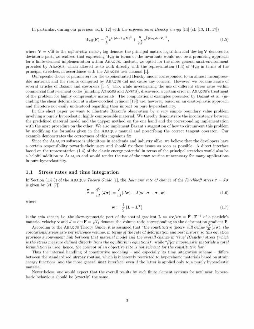
In particular, during our previous work [12] with the exponentiated Hencky energy [14] (cf. [13, 11, 17])

WeH(F) =µ

kek ‖dev log V‖2 +

κ

2 kek [(log detV)]2 , (1.5)

where V =√B is the left stretch tensor, log denotes the principal matrix logarithm and dev logV denotes its

deviatoric part, we realized that expressing WeH in terms of the invariants would not be a promising approachfor a finite-element implementation within Abaqus. Instead, we opted for the more general umat-environmentprovided by Abaqus, which allowed us to work directly with the representation (1.4) of WeH in terms of theprincipal stretches, in accordance with the Abaqus user manual [1].

Our specific choice of parameters for the exponentiated Hencky model corresponded to an almost incompress-ible material, and the results computed by Abaqus did not cause any concern. However, we became aware ofseveral articles of Bažant and coworkers [3, 9] who, while investigating the use of different stress rates withincommercial finite element codes (inluding Abaqus and Ansys), discovered a certain error in Abaqus’s treatmentof the problem for highly compressible materials. The computational examples presented by Bažant et al. (in-cluding the shear deformation at a skew-notched cylinder [18]) are, however, based on an elasto-plastic approachand therefore not easily understood regarding their impact on pure hyperelasticity.

In this short paper we want to illustrate Bažant’s observation by a very simple boundary value probleminvolving a purely hyperelastic, highly compressible material. We thereby demonstrate the inconsistency betweenthe predefined material model and the uhyper method on the one hand and the corresponding implementationwith the umat procedure on the other. We also implement Bažant’s suggestion of how to circumvent this problemby modifying the formulas given in the Abaqus manual and prescribing the correct tangent operator. Ourexample demonstrates the correctness of this ingenious fix.

Since the Abaqus software is ubiquitous in academia and industry alike, we believe that the developers havea certain responsibility towards their users and should fix these issues as soon as possible. A direct interfacebased on the representation (1.4) of the elastic energy potential in terms of the principal stretches would also bea helpful addition to Abaqus and would render the use of the umat routine unnecessary for many applicationsin pure hyperelasticity.

1.1 Stress rates and time integrationIn Section (1.5.3) of the Abaqus Theory Guide [1], the Jaumann rate of change of the Kirchhoff stress τ = Jσis given by (cf. [7])

∇τ =

d∇

dt(Jσ) :=

d

dt(Jσ)− J(w · σ − σ ·w) , (1.6)

wherew :=

1

2

(L− LT

)(1.7)

is the spin tensor, i.e. the skew-symmetric part of the spatial gradient L := ∂v/∂x = F · F−1 of a particle’smaterial velocity v and J = detF =

√I3 denotes the volume ratio corresponding to the deformation gradient F.

According to the Abaqus Theory Guide, it is assumed that “the constitutive theory will define d∇

dt (Jσ), thecorotational stress rate per reference volume, in terms of the rate of deformation and past history, so this equationprovides a convenient link between that material model and the overall change in ‘true’ (Cauchy) stress (whichis the stress measure defined directly from the equilibrium equations)”, while “ [f]or hyperelastic materials a totalformulation is used; hence, the concept of an objective rate is not relevant for the constitutive law.”

Thus the internal handling of constitutive modeling – and especially its time integration scheme – differsbetween the standardized uhyper routine, which is inherently restricted to hyperelastic materials based on strainenergy functions, and the more general umat interface, even if the latter is applied only to a purely hyperelasticmaterial.

Nevertheless, one would expect that the overall results by such finite element systems for nonlinear, hypere-lastic behaviour should be (exactly) the same.

3

2 Three ways of implementing hyperelasticity in Abaqus

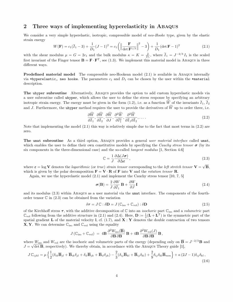
We consider a very simple hyperelastic, isotropic, compressible model of neo-Hooke type, given by the elasticstrain energy

W (F) = c1(I1 − 3) +1

D1(J − 1)2 = c1

(∥∥∥ F

detF1/3

∥∥∥2

− 3

)+

1

D1(detF− 1)2 (2.1)

with the shear modulus µ = G = 2c1 and the bulk modulus κ = K = 2D1

, where I1 = J−2/3 I1 is the scaledfirst invariant of the Finger tensor B = F ·FT, see (1.3). We implement this material model in Abaqus in threedifferent ways.

Predefined material model The compressible neo-Hookean model (2.1) is available in Abaqus internallyvia *hyperelastic, neo hooke. The parameters c1 and D1 can be chosen by the user within the *materialdescription.

The uhyper subroutine Alternatively, Abaqus provides the option to add custom hyperelastic models viaa user subroutine called uhyper, which allows the user to define the stress response by specifying an arbitraryisotropic strain energy. The energy must be given in the form (1.2), i.e. as a function W of the invariants I1, I2

and J . Furthermore, the uhyper method requires the user to provide the derivatives of W up to order three, i.e.

∂W

∂I1

,∂W

∂I2

,∂W

∂J,∂2W

∂I21

,∂2W

∂I1∂I2

, . . . . (2.2)

Note that implementing the model (2.1) this way is relatively simple due to the fact that most terms in (2.2) arezero.

The umat subroutine As a third option, Abaqus provides a general user material interface called umat,which enables the user to define their own constitutive models by specifying the Cauchy stress tensor σ (by itssix components in the three-dimensional case) and the so-called tangent modulus [1, Section 4.6]

C =1

J

∂∆(Jσ)

∂∆ε, (2.3)

where ε = logV denotes the logarithmic (or true) strain tensor corresponding to the left stretch tensor V =√B,

which is given by the polar decomposition F = V ·R of F into V and the rotation tensor R.Again, we use the hyperelastic model (2.1) and implement the Cauchy stress tensor [10, 7, 5]

σ(B) =2

J

∂W

∂I1

B +∂W

∂JI (2.4)

and its modulus (2.3) within Abaqus as a user material via the umat interface. The components of the fourth-order tensor C in (2.3) can be obtained from the variation

δτ = J C : δD = J (Ciso + Cvol) : δD (2.5)

of the Kirchhoff stress τ , with the additive decomposition of C into an isochoric part Ciso and a volumetric partCvol following from the additive structure in (2.1) and (2.4). Here, D := 1

2 (L + LT) is the symmetric part of thespatial gradient L of the material velocity l, cf. (1.7), and X : Y denotes the double contraction of two tensorsX,Y. We can determine Ciso and Cvol using the equality

J (Ciso + Cvol) = 4B∂2Wiso(B)

∂B ∂BB + 4B

∂2Wvol(J)

∂B ∂BB ,

where Wiso and Wvol are the isochoric and volumetric parts of the energy (depending only on B = J−2/3B andJ =√

detB, respectively). We thereby obtain, in accordance with the Abaqus Theory guide [1],

J Cijkl = µ1

2(δikBjl + Bikδjl + δilBjk + Bilδjk)− 2

3(δijBkl + Bijδkl) +

2

9δijδklBmm

+ κ (2J − 1)δijδkl ,

(2.6)

4

where δij is the Kronecker symbol for the second-order identity I, following the Einstein convention for summa-tion. An equivalent representation is given by Itskov [8]. Using (2.6) as well as (2.4), the neo-Hooke model (2.1)can now be implemented using the umat subroutine.

Remark 2.1. It is mentioned in the Abaqus Theory Guide [1] that, especially for “almost incompressible”materials, using the umat routine “ is suitable for material models that use an incremental formulation (forexample, metal plasticity) but is not consistent with a total formulation that is commonly used for hyperelasticmaterials.” Nevertheless, here we show the dramatic inconsistencies that arise from following the umat basedapproach for implementing (highly) compressible hyperelastic material behaviour.

In summary, we now have three different implementations of the neo-Hooke model (2.1) within Abaqus atour disposal: first the integrated material call, then the implementation via the uhyper routine and lastly theumat realization.

2.1 Bažant’s proposed modification of the tangent modulusIn addition to these three implementations, we also consider the modified tangent modulus

Cmodijkl = Cijkl − σijδkl , (2.7)

where C is given by (2.6) and σ = τ/J is the Cauchy stress tensor, which was proposed by Bažant [3, 9] tocompensate for the difference in results produced by Abaqus for different implementations. In order to comparethe numerical results, we implement the model with the umat subroutine again, this time using the modifiedmodulus Cmod

ijkl instead of C from (2.6).

3 Examples of numerical results for different implementationsUsing the different Abaqus implementations of our material model introduced in the previous section, we nowconsider two boundary value problems in order to highlight the discrepancies between the results.

casing

28 mm ∅ 2 mmgroove

MPa

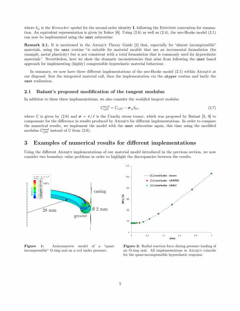
Figure 1: Axisymmetric model of a “quasi–incompressible” O-ring seal on a rod under pressure.

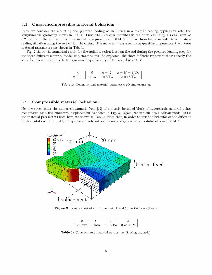
Figure 2: Radial reaction force during pressure loading ofan O-ring seal. All implementations in Abaqus coincidefor the quasi-incompressible hyperelastic response.

5

3.1 Quasi-incompressible material behaviourFirst, we consider the mounting and pressure loading of an O-ring in a realistic sealing application with theaxisymmetric geometry shown in Fig. 1. First, the O-ring is mounted in the outer casing by a radial shift of0.25 mm into the groove. It is then loaded by a pressure of 5.0 MPa (50 bar) from below in order to simulate asealing situation along the rod within the casing. The material is assumed to be quasi-incompressible; the chosenmaterial parameters are shown in Tab. 1.

Fig. 2 shows the numerical result for the radial reaction force on the rod during the pressure loading step forthe three different material model implementations. As expected, the three different responses show exactly thesame behaviour since, due to the quasi-incompressibility, J ≈ 1 and thus σ ≈ τ .

ri d µ = G κ = K = 2/D1

28 mm 2 mm 1.0 MPa 2000 MPa

Table 1: Geometry and material parameters (O-ring example).

3.2 Compressible material behaviourNext, we reconsider the numerical example from [12] of a mostly bounded block of hyperelastic material beingcompressed by a flat, unilateral displacement as shown in Fig. 3. Again, we use our neo-Hookean model (2.1);the material parameters used here are shown in Tab. 2. Note that, in order to test the behavior of the differentimplementations for a highly compressible material, we choose a very low bulk modulus of κ = 0.78 MPa.

MPa

5 mm, fixed

displacement

20 mm20 mm

Figure 3: Square sheet of a = 20 mm width and 5 mm thickness (fixed).

a t µ κ20 mm 5 mm 1.0 MPa 0.78 MPa

Table 2: Geometry and material parameters (footing example).

6

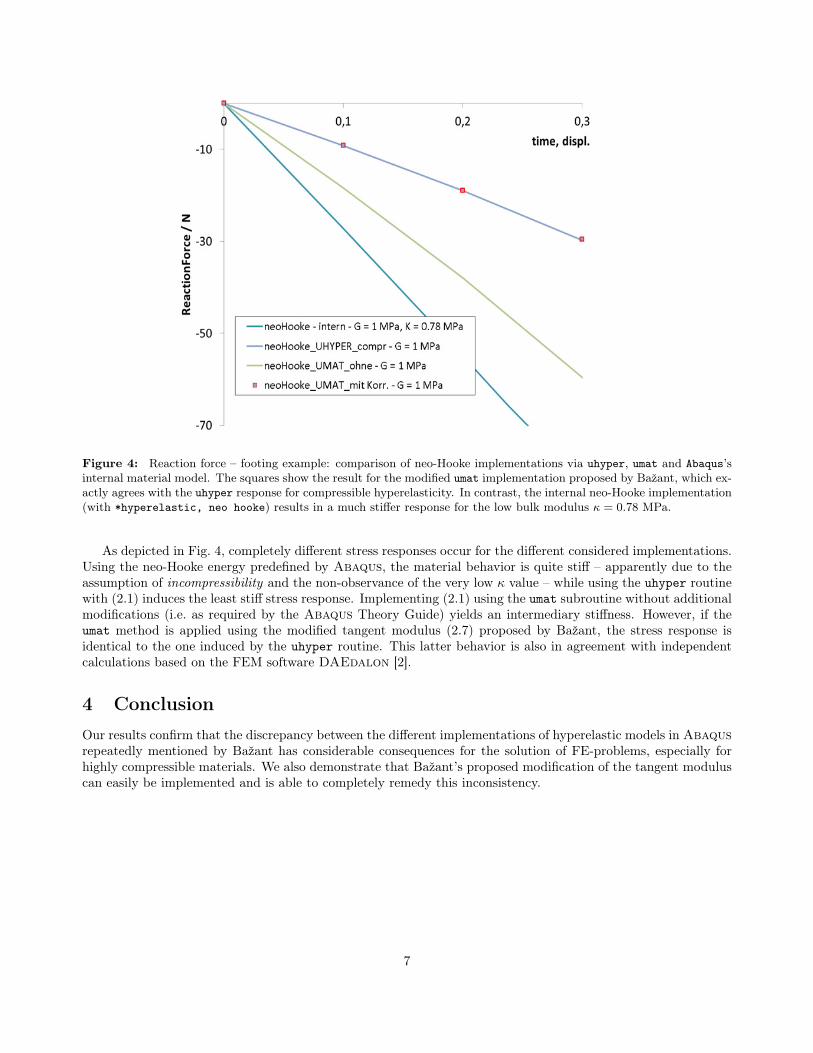
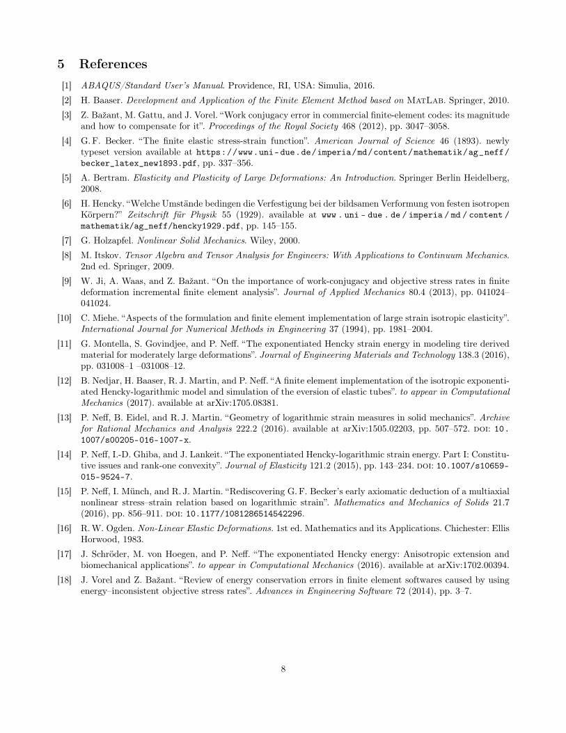
Figure 4: Reaction force – footing example: comparison of neo-Hooke implementations via uhyper, umat and Abaqus’sinternal material model. The squares show the result for the modified umat implementation proposed by Bažant, which ex-actly agrees with the uhyper response for compressible hyperelasticity. In contrast, the internal neo-Hooke implementation(with *hyperelastic, neo hooke) results in a much stiffer response for the low bulk modulus κ = 0.78 MPa.

As depicted in Fig. 4, completely different stress responses occur for the different considered implementations.Using the neo-Hooke energy predefined by Abaqus, the material behavior is quite stiff – apparently due to theassumption of incompressibility and the non-observance of the very low κ value – while using the uhyper routinewith (2.1) induces the least stiff stress response. Implementing (2.1) using the umat subroutine without additionalmodifications (i.e. as required by the Abaqus Theory Guide) yields an intermediary stiffness. However, if theumat method is applied using the modified tangent modulus (2.7) proposed by Bažant, the stress response isidentical to the one induced by the uhyper routine. This latter behavior is also in agreement with independentcalculations based on the FEM software DAEdalon [2].

4 ConclusionOur results confirm that the discrepancy between the different implementations of hyperelastic models in Abaqusrepeatedly mentioned by Bažant has considerable consequences for the solution of FE-problems, especially forhighly compressible materials. We also demonstrate that Bažant’s proposed modification of the tangent moduluscan easily be implemented and is able to completely remedy this inconsistency.

7

5 References[1] ABAQUS/Standard User’s Manual. Providence, RI, USA: Simulia, 2016.

[2] H. Baaser. Development and Application of the Finite Element Method based on MatLab. Springer, 2010.

[3] Z. Bažant, M. Gattu, and J. Vorel. “Work conjugacy error in commercial finite-element codes: its magnitudeand how to compensate for it”. Proceedings of the Royal Society 468 (2012), pp. 3047–3058.

[4] G. F. Becker. “The finite elastic stress-strain function”. American Journal of Science 46 (1893). newlytypeset version available at https://www.uni-due.de/imperia/md/content/mathematik/ag_neff/becker_latex_new1893.pdf, pp. 337–356.

[5] A. Bertram. Elasticity and Plasticity of Large Deformations: An Introduction. Springer Berlin Heidelberg,2008.

[6] H. Hencky. “Welche Umstände bedingen die Verfestigung bei der bildsamen Verformung von festen isotropenKörpern?” Zeitschrift für Physik 55 (1929). available at www . uni - due . de / imperia / md / content /mathematik/ag_neff/hencky1929.pdf, pp. 145–155.

[7] G. Holzapfel. Nonlinear Solid Mechanics. Wiley, 2000.

[8] M. Itskov. Tensor Algebra and Tensor Analysis for Engineers: With Applications to Continuum Mechanics.2nd ed. Springer, 2009.

[9] W. Ji, A. Waas, and Z. Bažant. “On the importance of work-conjugacy and objective stress rates in finitedeformation incremental finite element analysis”. Journal of Applied Mechanics 80.4 (2013), pp. 041024–041024.

[10] C. Miehe. “Aspects of the formulation and finite element implementation of large strain isotropic elasticity”.International Journal for Numerical Methods in Engineering 37 (1994), pp. 1981–2004.

[11] G. Montella, S. Govindjee, and P. Neff. “The exponentiated Hencky strain energy in modeling tire derivedmaterial for moderately large deformations”. Journal of Engineering Materials and Technology 138.3 (2016),pp. 031008–1 –031008–12.

[12] B. Nedjar, H. Baaser, R. J. Martin, and P. Neff. “A finite element implementation of the isotropic exponenti-ated Hencky-logarithmic model and simulation of the eversion of elastic tubes”. to appear in ComputationalMechanics (2017). available at arXiv:1705.08381.

[13] P. Neff, B. Eidel, and R. J. Martin. “Geometry of logarithmic strain measures in solid mechanics”. Archivefor Rational Mechanics and Analysis 222.2 (2016). available at arXiv:1505.02203, pp. 507–572. doi: 10.1007/s00205-016-1007-x.

[14] P. Neff, I.-D. Ghiba, and J. Lankeit. “The exponentiated Hencky-logarithmic strain energy. Part I: Constitu-tive issues and rank-one convexity”. Journal of Elasticity 121.2 (2015), pp. 143–234. doi: 10.1007/s10659-015-9524-7.

[15] P. Neff, I. Münch, and R. J. Martin. “Rediscovering G. F. Becker’s early axiomatic deduction of a multiaxialnonlinear stress–strain relation based on logarithmic strain”. Mathematics and Mechanics of Solids 21.7(2016), pp. 856–911. doi: 10.1177/1081286514542296.

[16] R.W. Ogden. Non-Linear Elastic Deformations. 1st ed. Mathematics and its Applications. Chichester: EllisHorwood, 1983.

[17] J. Schröder, M. von Hoegen, and P. Neff. “The exponentiated Hencky energy: Anisotropic extension andbiomechanical applications”. to appear in Computational Mechanics (2016). available at arXiv:1702.00394.

[18] J. Vorel and Z. Bažant. “Review of energy conservation errors in finite element softwares caused by usingenergy–inconsistent objective stress rates”. Advances in Engineering Software 72 (2014), pp. 3–7.

8