Embed Size (px)
Citation preview
Incorporating Climate Change Feedbacks into a General Economic Equilibrium Model
Sergey Paltsev and John Reilly
Joint Program on the Science and Policy of Global Change
Massachusetts Institute of Technology, Cambridge, MA 02139, USA Abstract:
To incorporate market and non-market effects of climate change into a computable general equilibrium (CGE) model, we begin with the basic data that supports CGE models, the Social Accounting Matrix (SAM). We identify where environmental damage appears in these accounts, estimate the physical loss, and value the loss within this accounting structure. Our approach is an exercise in environmental accounting, augmenting the standard national income and product accounts to include environmental damage. Examples of applying the approach in two areas are provided: air pollution health effects and economy-atmosphere-land-agriculture interactions.
We estimate market and non-market effects of air pollution on human health for the U.S. for the period from 1970 to 2000. The pollutants include tropospheric ozone, nitrogen dioxide, sulfur dioxide, carbon monoxide, and particulate matter. The health effects from exposure to air pollution are integrated into the MIT Emissions Prediction and Policy Analysis (EPPA) model, a computable general equilibrium model of the economy that has been widely used to study climate change policy. Benefits of air pollution regulations in USA rose steadily from 1975 to 2000 from $50 billion to $400 billion (from 2.1% to 7.6% of market consumption). We also estimate the economic burden of uncontrolled levels of air pollution over that period. In another case study, we examine the health-related economic benefits and costs of policy actions for China. We found that economic burden of uncontrolled levels of air pollution is lower that in the U.S. because of lower wage rates but macroeconomic impact is bigger than in the U.S. (in 2000 the economic burden in the USA is 4.7% of market consumption, in China - it is 10% of market consumption).
For assessing the impacts of environmental change on vegetation (crop productivity, forest productivity, pasture), we have augmented the EPPA model by further disaggregating the agricultural sector. This allows us to simulate economic effects of changes in yield (i.e., the productivity of cropland) on the regional economies of the world, including impacts on agricultural trade. We examine multiple scenarios where tropospheric ozone precursors are controlled or not, and where greenhouse gas emissions are abated or not. In general, a change in food consumption is smaller than a change in agriculture yield due to resource reallocation from or to the rest of the economy. ____ The paper is prepared for the Ninth Annual Conference on Global Economic Analysis in Addis Ababa, Ethiopia (June 15-17, 2006). We thank many of our colleagues and students in the MIT Joint Program. Their supportive comments, suggestions and research assistance have greatly improved the EPPA model and its applications.

2
1. Introduction
General equilibrium analysis accounts for the intersectoral reallocation of
resources that could occur as a consequence of climate change. A key strength of
Computable General Equilibrium (CGE) models is their ability to model economy-wide
effects of policies and other external shocks, rather than just on individual markets or
sectors. In this paper we present a methodology for incorporating market and non-market
effects of climate change into a CGE model. We begin with the basic data that supports
CGE models, the Social Accounting Matrix (SAM) that includes the input-output tables
of an economy, the use and supply of factors, and the disposition of goods in final
consumption. We identify where environmental damage appears in these accounts,
estimate the physical loss, and value the loss within this accounting structure. Our
approach is an exercise in environmental accounting, augmenting the standard national
income and product accounts to include environmental damage.
We provide examples of applying our approach in two areas: air pollution health
effects and economy-atmosphere-land-agriculture interactions. We integrate the health
effects from exposure to air pollution into the MIT Emissions Prediction and Policy
Analysis (EPPA) model (Paltsev et al., 2005), a computable general equilibrium model of
the economy that has been widely used to study climate change policy. We apply the
model to estimate the benefits of air pollution regulations and the economic burden
uncontrolled levels of air pollution in USA in China for 1975 to 2000.
Agriculture is another area where environmental change is likely to have
important effects. Multiple changes that may occur over the next century will affect
vegetation (crop productivity, forest productivity, pasture). Some of these effects are

3
likely to be positive (CO2 fertilization), some negative (tropospheric ozone damage), and
some may be either positive or negative (temperature and precipitation). Climate effects
may operate in either direction because the direction of change may differ across regions
(more precipitation in some areas and less in others) and warming may increase growing
season lengths in cold-limited growing areas while acting as a detriment to productivity
in areas with already high temperatures. Here we use the MIT Integrated Global Systems
Model (IGSM) (Sokolov et al., 2005) to analyze the economic impact of environmental
change effects on vegetation. For this work we have augmented the EPPA model by
further disaggregating the agricultural sector. This allows us to simulate economic effects
of changes in yield (i.e., the productivity of cropland) on the regional economies of the
world, including impacts on agricultural trade. The EPPA model includes multiple
channels of market-based adaptation, including input substitution and trade. We are thus
able to examine the extent to which market forces contribute toward adaptation and thus
modify the initial yield effects.
In the next section we describe a basic structure of a SAM and discuss a link
between economic value and supplemental physical flows. Section 3 presents the changes
in the SAM and the structure of our CGE model, which we have made to assess the
health impacts of air pollution. We also provide our estimates of the benefits of air
pollution regulations and the economic burden uncontrolled levels of air pollution in
USA in China for 1975 to 2000. In Section 4 we then provide a description of the
changes in the model structure for the analysis of climate change impacts on agriculture.
We examine several scenarios where tropospheric ozone precursors are controlled or not,
and where greenhouse gas emissions are abated or not, and show the impacts on

4
agriculture yield, food consumption and total macroeconomic consumption. Section 5
concludes.
2. Expanded Social Accounting Matrix and Linkage to Physical Flows
Data for a particular country or region are often organized in the form of a Social
Accounting Matrix (SAM), which presents a static image of the economy. The
information contained in the SAM provides a basis for the creation of a plausible CGE
model. A SAM describes the flows among the various sectors of the economy. It
represents the value of economic transactions in a given period of time. Transactions of
goods and services are broken down by intermediate and final use. A SAM also shows
the cost structure of production activities: intermediate inputs, compensation to labor and
capital, taxes on production. Figure 1 illustrates a general structure of a SAM, where
Matrix A represents an intermediate demand. Rows in the matrix A describe production
sector outputs. Columns represent sectors which use outputs of production as
intermediate inputs. As such, a number in a cell Aij tells the amount of sector i's output
used in the production of a sector j. A breakdown of a final demand on private
consumption, government consumption, investment, and export is shown in Matrix B.
Matrix C gives the information on total domestic production. Matrices D, E and F give
the corresponding information on imported goods and services. Payments to labor and
capital, depreciation, and indirect taxes are presented in Matrix G. Matrix H is normally
empty, and summation over rows in Matrix I gives information on value-added. If a SAM
is balanced, then columns of Matrix J should be the same as the rows of Matrix C
because total input equals total output for production sectors.

5
A SAM illustrates the circular process of demand leading to production leading to
income, which in turn leads back to demand. There is an exact correspondence between
rows and columns in a balanced SAM. This means that supply equals demand for all
goods and factors, tax payments equals tax receipts, there are no excess profits in
production, the value of each household expenditure equals the value of factor income
plus transfers, and the value of government tax revenue equals the value of transfers.
To build a CGE model, a modeler needs additional information on elasticities of
substitution between inputs in production and between goods in consumption. A SAM
does not provide this information. For importance of information on elasticity of
substitution for building a CGE model see Rutherford (1995). Another choice for a CGE
modeler is a structure of production and consumption bundles (i.e., a nesting structure of
substitution possibilities) and functional forms for production and utility functions. In this
paper we use the elasticities, nesting structures, and functional forms of the EPPA4
model as documented in Paltsev et al. (2005). We do not repeat them here, but we discuss
the changes and additions to the EPPA production and consumption structure we use for
incorporating climate change feedbacks in the consecutive sections.
The first step is to identify where environmental damage appears in a SAM,
estimate the physical loss, and value the loss within this accounting structure. For health
effects, one needs to account for lost productivity, a decrease in labor force, and changes
in expenditure in the health sector at the expense of other sector of the economy. For
agriculture productivity effects, one needs to keep track of land use database, to estimate
the changes in vegetation due to changed climate and pollution, and to introduce these
agriculture productivity changes back into an economic system. For a sea-level change,

6
which would affect the quantity and the value of land, an additional database on the area
and value of the coastal land, and estimates of protection of urban and agricultural land,
as well as costs of relocation of agriculture and urban areas are needed.
In many cases, it is important to include supplemental accounting of physical and
biological variables. For example, in EPPA we use such supplemental tables for physical
energy use, as they are necessary for accounting of carbon dioxide emissions and tracking
of physical depletion of energy resources. For impact on agriculture we disaggregate
agriculture to explicitly treat land use and feedbacks impacts on vegetation.
A SAM provides the data in value form, i.e., using total expenditure or sales as a
measure of the quantity of inputs and outputs in the economy. That is, these data do not
report quantities in tons of wheat, coal, iron ore, or steel produced or the hectares of land,
hours of labor, or exajoules of energy used to produce them. Instead they report the total
expenditure on energy or labor, rental payments to land and capital, and the total sales or
purchases of goods and services.
Measuring inputs and outputs in terms of expenditure or of the total value of sales
greatly facilitates aggregation. The economic theory underlying this practice holds that
the prices of goods reflect their marginal value as inputs into production or of
consumption.1 Different prices for varying grades of a particular commodity thus reflect
their differential value as a production input or for consumption. One might ideally desire
a fine disaggregation of inputs and outputs, but of course there are different varieties and
1 Problems of aggregation are eliminated in a base year, but they resurface when comparisons of real economic growth are to be made over time. One then must worry about the quality (and implicitly) the mix of products of different qualities in any aggregation. Much economic work has been devoted to creating prices indices that capture accurately the changing mix, but there remain difficult problems of changing quality that bedevil efforts to identify real growth and changes in the price level. To solve these problems requires going back to more fundamental and disaggregated observations.

7
grades of even such basic commodities as, for example, apples, wheat, coal or crude oil.
Similarly, the labor force is composed of individuals with widely varying skills, and land
has a wide range of characteristics that are more or less useful for different purposes. In
manufacturing and services, product differentiation is the rule rather than the exception,
and no one would believe it made much sense to measure hair cuts and financial services
in their natural units and add them together.
In economic models the problem of adding together apples and oranges (or
different varieties of apples) is solved by using price weights. For example, consider a
land owner with three different parcels of land: parcel #1 is 300 hectares and rents for
$75 per hectare, parcel #2 is 150 hectares and rents for $150 per hectare, and parcel #3 is
75 hectares and rents for $300 hectare. Most people would sum together the hectares and
conclude that the total land owned is 525 hectares. Economists are interested, however, in
the contribution this land makes to the economy, and they would thus observe that parcel
#2 is twice as valuable per hectare as parcel #1, and parcel #3 twice as valuable as parcel
#2. They use the rental value as an appropriate weight to sum these together. Parcel 1’s
annual value to the economy is $75 x 300= $22,500; parcel 2 is $150 x 150 =$22,500,
and parcel 3 is $300 x 75 =$22,500. The example here is constructed so that when
weighted by price, the three parcels are equal in size in terms of their input into the
economy, which is a very different conclusion than using hectares directly which would
indicate that parcel #1 is four times bigger than parcel #3.
The approach of weighting inputs and products by their marginal value allows
agricultural or steel production or energy input to be aggregated in an economically
meaningful manner. Agriculture output is composed of commodities like corn, wheat,

8
beef, lamb, apples, oranges, raspberries, and asparagus. It would be nonsensical to add
together total tons because that would mean that fruit and vegetable production is a minor
component of agriculture when in value terms it is as important as grain crops. Output of
the iron and steel industry includes specialty alloy products, cast iron, and more common
sheet or bar products. Similarly, an exajoule of coal is of less value to the economy than
an exajoule of oil, gas, or electricity.
Formally, a CGE model such as EPPA measures all inputs and outputs in the
economy in billions of dollars. Given the use of value as the quantity measure, all prices
are unit-less (=1.0) in the base year and so when multiplied times the input quantity one
then gets back expenditure or income as a monetary measure.2 Simulating the model
forward, or in a counterfactual case, is a process of finding prices that clear the markets
given some exogenous change or limitation on how the economy can use its resources.
Market-clearing prices in these simulations will typically vary from 1.0. If, for example,
the labor force is estimated to increase by 20% from $10 billion this will be simulated as
a labor input of $12 billion. The base year wage rate is defined as 1.0 and so wage
income (and the wage bill for employers in the economy) is $10 billion in the base year.
But in the future year if the market clearing wage rate falls to 0.95 relative to the
numeraire good then labor income will have increased by 0.95 x $12 billion =$11.4 or
only 14% but we still measure the “physical” increase in labor to be the 20% increase
from $10 to $12 billion.
If the focus is on purely economic results over the short and medium term, this
approach to economic modeling has proven useful. Changes in physical inputs are
implied by economic modeling but are not explicitly tracked. The limitation of this 2 For an introduction to the analytic procedures underlying CGE models see Sue Wing (2004).

9
approach for earth system and longer-term economic modeling is that there is no
straightforward way to keep track of important physical flows such as emissions of
pollutants, depletion of resources, changes in land use, and the efficiency of physical
processes such as conversion of fuels to electricity. This feature further limits the use of
engineering data on new technologies. For example, the electric sector data includes
multiple fuels, capital, labor, and intermediate inputs that lead to the fossil-based
production and transmission of electricity, but also includes technologies such as nuclear
and hydroelectric power that do not use fossil fuels. Engineering cost data for new
electricity technologies such as wind, natural gas combined cycle, or integrated coal
gasification with sequestration typically focus on generation cost rather than the broader
costs of running an electric utility company and transmitting and distributing the product.
Moreover, an aggregate electricity sector that includes both fossil sources and hydro,
nuclear, and other renewable sources cannot be evaluated directly to determine the
efficiency of energy conversion. Engineering estimates of future efficiency of conversion
and the technological costs of key options as they depend on resource availability and
quality is useful information that can help constrain and inform longer run economic-
energy forecasts. Finally, one must also recognize that environmental feedbacks on the
economy through changes in the productivity of crops and forests and impacts on the
human population will be mediated through impacts on physical systems. For all of these
reasons it is essential in climate analysis to link the changes in the physical and biological
environment of the earth system to the underlying economic variables.

10
3. Health Effects
The conventional approach to estimating health damage from air pollution is to
multiply a predicted illness or death by a constant value meant to capture the value of lost
life or the cost of the health care. However, health costs do not affect the overall economy
equally. When people get sick and miss work, their lost productivity will negatively
affect certain sectors. In addition, people buy medicine and use medical services, an
expenditure that will require more resources to be used in the health sector at the expense
of other sectors. People sometimes get ill not due to air pollution levels in a single day or
year but rather due to their lifetime exposures to pollutants. And if people die
prematurely due to pollution exposure, their contribution to the workforce is lost in every
year from their death until their normal retirement date.
To reflect these complexities in a CGE model, several steps are needed:
1. The model should be able to generate an estimate of emissions depending on the
changes in economic activity (this step is needed for projections into the future);
2. The air pollution model should be able to convert these emissions into concentrations,
because the existing epidemiological estimates reflect health impacts due to a change in a
concentration of a pollutant, not to a change in emissions (this step is needed for
projections into the future);
3. Expand SAM to include valuation of health effects;
4. Create a production structure for a pollution health service;
5. Get epidemiological estimates of the relationships between air pollution and health;
6. Create relationships on lost labor, leisure, and increase/reduction in medical services;

11
7. Run the model with a scenario of pollution without air-pollution policy, a scenario with
air pollution policy, and a scenario with a “natural” pollution, and compare the results;
Steps 1 and 2 are not needed if one tries to estimate the effects of historic regulations
and the data on pollutant concentrations are available. For more details on these steps see
Matus et al. (2006). Here we focus on presentation of the changes in the SAM and CGE
structure. Extending the model to included health effects involves valuation of non-wage
time (leisure) and inclusion of a household production of health services, which we
represent in a SAM as shown in Figure 2. The extensions of model are highlighted in
italic bold. We add a household service sector that provides a ‘pollution health service’ to
final consumption to capture economic effects of morbidity and mortality from acute
exposure. This household service sector is shown as ‘household mitigation of pollution
health effects.’ It uses ‘medical services’ (i.e., hospital care and physician services) from
the SERV sector of EPPA and household labor to produce a health service. The
household labor is drawn from labor and leisure and thus reduces the amount available
for other uses; i.e., an illness results in purchase of medical services and/or patient time to
recover when they cannot work or participate in other household activities. We use data
from traditional valuation work to estimate the amount of each of these inputs for each
health endpoint as discussed in the following sections. Changed pollution levels are
modeled as a Hick’s neutral technical change: higher pollution levels require
proportionally more of all inputs to deliver the same level of health service, or lower
levels require proportionally less.3
3 Modeled here as a negative technical change, greater expenditure due to more pollution draws resources from other uses and thus reduces consumption of other goods and leisure—more pollution is thus bad. The increased expenditures combat the pollution effects, and do not increase consumption and welfare. Of course, greater expenditure for a fixed level of pollution will generate more health benefits.
12
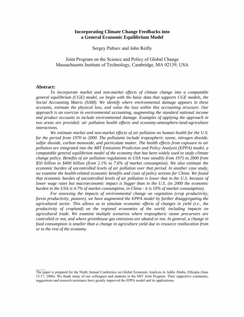
As presented in Figure 3, the EPPA model includes 16 countries/regions, 6 non-
energy sectors, and 15 energy sectors/technologies., but the model does not have
household production sector. Figure 4 shows the household service (production) structure
with the added components in bold italics. The key new additions are (1) leisure as a
component of consumption and (2) the Household Healthcare (HH) sector that includes
separate production relationships for health effects of each pollutant. The elasticity, σL, is
parameterized to represent a labor own-price supply elasticity typical of the literature, as
discussed in more detail later. The HH sector is Leontief in relationship to other goods
and services and among pollutant health endpoints. Mortality effects simply result in a
loss of labor and leisure, and thus are equivalent to a negative labor productivity shock.
Impacts on health are usually estimated to be the largest air pollution effects when
measured in economic terms using conventional valuation approaches, dominating other
losses such as damage to physical infrastructure, crops, ecosystems and loss of visibility
(e.g., US Environmental Protection Agency, 1999). The health effects of air pollution
present themselves as both a loss of current well-being (an illness brought on by acute
exposure to air pollution that results in temporary hospitalization or restricted activity)
and as an effect that lasts through many periods (years of exposure that eventually lead to
illness, and deaths where losses to society and the economy extend from the point of
premature death forward until that person would have died of other causes had they not
been exposed to pollution). Thus, we are faced with accounting both for stocks and flows
of labor endowment in the economy and the population’s exposure to pollution. Health
effects also present themselves as both market and non-market effects. Death or illness of
someone in the labor force means that person’s income is no longer part of the economy,
13
clearly a market effect. Illness also often involves expenditure on medical services,
counted as part of the market economy. Death and illness also involve loss of non-paid
work time, a non-market impact. This likely involves a loss of time for household chores
or a loss of time spent on leisure activities. The health effects area thus is both a large
component of total air pollution damages and provides an opportunity to develop
methods to handle a variety of issues faced in valuing changes in environmental
conditions.
Epidemiological relationships have been estimated for many pollutants, as they
relate to a variety of health impacts. The work has been focused on a set of substances
often referred to as ‘criteria pollutants,’ so-called because the U.S. EPA developed
health-based criteria as the basis for setting permissible levels. These same pollutants are
regulated in many countries. For more on epidemiological relationships that we use in our
study, see Matus et al. (2006).
As presented in Figure 5, the benefits from air pollution regulation in USA rose
steadily from 1975 to 2000 by our estimate. In terms of additional market consumption +
leisure, the benefits rose steadily from 1975 to 2000 from around 50 billion of 1997 USD
to 400 billion of 1997 USD. It is worthwhile to note that in the expanded accounting a
true willingness to pay estimate of benefits should be income constrained. In our
approach, benefits are not necessarily constrained by market income but by the total
resources available to the household including market income plus the value of leisure.
Faced with illness or death to a member, households will use their non-market resources
as well as income to combat the disease, and thus exhibit a willingness to pay (or use)
these resources.

14
Figure 5 also shows the remaining costs of pollution over the period of 1975-
2000. The results are less dependent on a projection of a counter-factual case. Essentially,
background levels of pollution are so low that slightly different assumptions about
background levels would have little effect on our estimates. Because the actual pollution
levels are falling over time, due to regulations, exposure to pollution per person is falling.
This alone would reduce pollution costs over time. The urban population is growing
slowly, but the more important factor is that the economy and wage rates are growing
over the period. As the value of lost work and leisure rise over time, the absolute
economic cost of pollution actually rises slightly over the entire period, despite a
substantial decrease in the level of pollution.
In another case study, we examine the health-related economic benefits and costs
of policy actions for China, as presented in Figure 6. We found that economic burden of
uncontrolled levels of air pollution is lower that in the U.S. because of lower wage rates
but macroeconomic impact is bigger than in the U.S. (in 2000 the economic burden in the
USA is 4.7% of market consumption, in China - it is 10% of market consumption).
For more information on benefits and costs by pollutant and a sensitivity analysis
see Matus et al. (2005) and Matus et al. (2006).
4. Agriculture Effects
Agriculture is another area where environmental change is likely to have important
effects. Multiple changes that may occur over the next century will affect vegetation
(crop productivity, forest productivity, pasture). Some of these effects are likely to be
positive (CO2 fertilization), some negative (tropospheric ozone damage), and some may

15
be either positive or negative (temperature and precipitation). Climate effects may
operate in either direction because the direction of change may differ across regions
(more precipitation in some areas and less in others) and warming may increase growing
season lengths in cold-limited growing areas while acting as a detriment to productivity
in areas with already high temperatures.
The steps we have done to focus on the vegetation and economic effects of climate
and ozone are as follows:
1. Disaggregate agriculture sector.
2. Get a separate food sector.
3. Get estimates on pollution in agriculture yield.
4. Run Business-As-Usual and other scenarios.
Here we use the MIT Integrated Global Systems Model (IGSM) to analyze the
economic impact of environmental change effects on vegetation, in particular its TEM
component, which is a process based biogeochemistry model that simulates the cycling of
carbon, nitrogen, and water among vegetation, soils, and the atmosphere. For this work
we have augmented the EPPA model by further disaggregating the agricultural sector.
This allows us to simulate economic effects of changes in yield (i.e., the productivity of
cropland) on the regional economies of the world, including impacts on agricultural trade.
The EPPA model includes multiple channels of market-based adaptation, including input
substitution and trade. We are thus able to examine the extent to which market forces
contribute toward adaptation and thus modify the initial yield effects. We examine
multiple scenarios where tropospheric ozone precursors are controlled or not, and where

16
greenhouse gas emissions are abated or not. This allows us to consider how these policies
interact. For more information on this study, see Reilly et al. (2006).
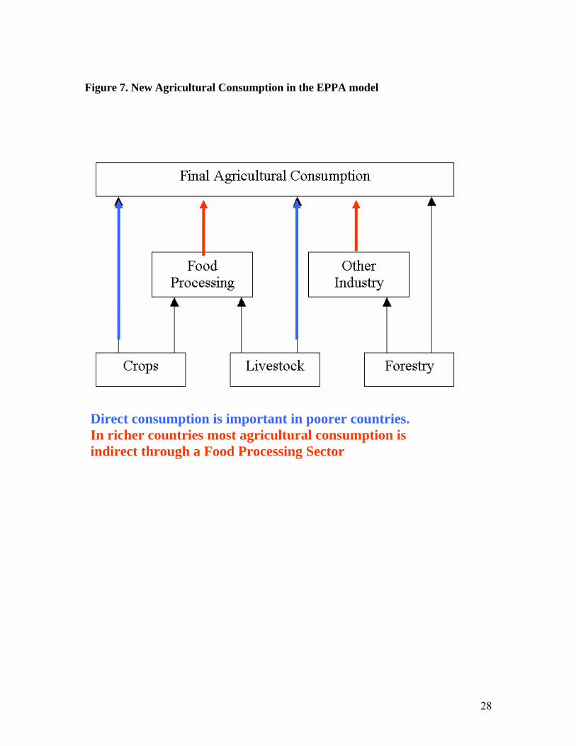
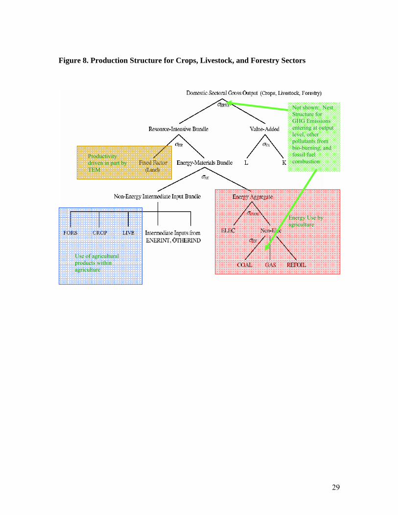
In a SAM we change a productivity of land, which would be reflected in the value
added for natural resources on Figure 1. We also disaggregate food processing sector and
change the structure of crop, livestock, and forestry sectors as presented on Figures 7-9.
We consider the following scenarios.
High Pollution: There are no efforts to control emissions of greenhouse gases (GHGs).
Emissions coefficients per unit of combustion for other pollutants decline in different
regions as incomes increase based on cross-section estimates of the relationship
between per capita income. The decline is estimated separately for each pollutant, and
for different combustion sources including large point source, small sources, and for
households. In principle, this would tend to create an environmental Kuznets’ curve
relationship, but the exhibited decline in emissions per unit of fuel combustion is
insufficient to offset increases in use of fuels, and so pollution levels rise
substantially.
Climate and GHGs only: The same climate and pollution scenario as the High Pollution
case but with the ozone damage mechanism in TEM turned off so that we can observe
the climate and CO2 effects alone without the effect of ozone damage.
Capped pollution: Conventional pollutants (CO, VOC, NOx, SO2, NH3, black carbon,
and organic carbon) are capped at 2005 levels, but GHG emissions remain
uncontrolled. The major effect of capping these pollutants is to reduce ozone levels
because many of these are important ozone precursors and thus ozone damage to
vegetation is reduced. The climate effects of reducing these pollutants are small

17
because of the offsetting effects from different pollutants. Sulfates are cooling
substances so reducing them tends to increase the temperature but ozone is a warming
substance and so reducing ozone precursors leads to less warming.
GHGs capped: Greenhouse gases are controlled along a path that starts with the Kyoto
Protocol, deepening the cuts in developed countries and expanding to include
developing countries on a pathway that keeps CO2 concentrations below 550 ppm by
2100 and with continued emissions reduction that could be consistent with
stabilization of concentrations at 550 ppm. This scenario is described in Reilly et al.
(1999). Because combustion of fossil fuels is affected, this scenario also leads to
significant reduction from reference of other pollutants including ozone precursors.
GHGs capped-no ozone: The same climate and GHG levels as in the GHGs capped
scenario but with the ozone damage mechanism in the TEM model again turned off
so that we can observe the climate and CO2 effects alone without the effect of ozone
damage.
GHGs and pollution capped: GHGs controlled as in the GHGs capped scenario and
conventional pollutants capped as in the Capped pollution scenario.
We focus first on global effects on production of these yield changes. To
effectively compare the global production effects with the yield changes, we construct a
measure of global yield change for crops, pasture, and forestry derived from TEM to
compare with estimated production change once we simulate the effect of these changes
in EPPA. The global yield changes are derived by summing the total level of
agroecosystem productivity (gC/year) for the globe and calculating the difference from

18
2000, as we did for each of the regions. Thus, the percentage change is weighted by the
absolute productivity in different regions. The global sector production (crop, livestock,
forestry) is measured in the total value of production in real terms in 1997 US dollars and
at 1997 market exchange rates as reported in EPPA. We calculate the difference from the
reference projection (without environment effects) to measure the effect on production of
each of the environmental change in terms of sector production levels. These are plotted
in Figures 10-12. For exposition, we have not plotted the GHGs capped-no ozone
scenario because it is very similar to GHGs and pollution capped scenario.
Figure 10 reports the results for crops. As expected, positive (negative) yield
effects of environmental change lead to positive (negative) production effects. However,
note that the production effects are far smaller than the yield effects. The global yield
effects are for an increase of over 60 percent (Climate and GHGs only) to a decline of
nearly 40 percent (High pollution) while the crop production effects are no larger than ±
8 percent. This reflects relative inelastic demand for crops because of a relatively
inelastic demand for food, the ability to substitute other inputs for land (adapt), and the
ability to shift land into or out of crops.
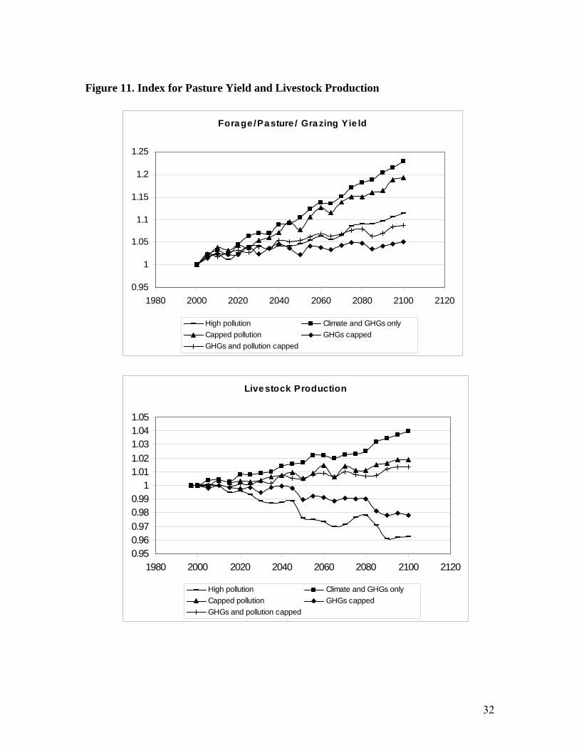
Figure 11 reports results for livestock. Here the livestock production results bear
little relationship to the yield effects for pasture. The pasture results are all positive
whereas several of the scenarios show reductions in livestock production. In fact, the
scenarios mirror closely the production effects on crops. This reflects the fact that
feedgrains and other crops are important inputs into livestock production, relatively more
important than pasture. A reduction (increase) in crop production is reflected in higher
(lower) prices for feedgrains and other crops used in livestock, and this tends to lead to

19
reduced (increased) production of livestock. Again, the percentage differences in
livestock production are relatively small compared with the crop production changes,
even in cases where production increases are driven both by an increase in crop
production and an increase in pasture productivity.
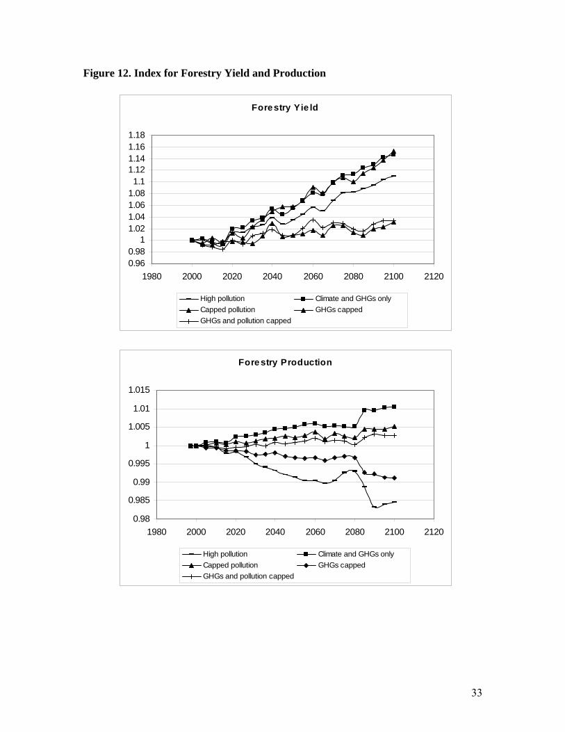
Figure 12 reports results for forestry. The general result is that the production
effects are very small—less than 1 percent compared with yield effects of 3 to 15 percent.
An important result of the general equilibrium modeling of these impacts is that
effects can be felt beyond the agricultural sector. We show this in Figure 13 where we
have plotted macroeconomic consumption change and the change in food consumption
both as a percent of food consumption in a reference case where there is no
environmental feedback on the economy. To illustrate this effect, we present the results
for two scenarios – High pollution and Climate and GHGs only, because those are the
ones that show the biggest change. This shows that, in general, the aggregate
consumption effect is bigger in absolute terms than the agricultural production effect.
Thus, adaptation in the agricultural sector which was seen most clearly in the crop sector
results, but by the general result that the production effects were much smaller than the
yield effects, is partly the result of shifting of resources into or out of these sectors,
thereby affecting the rest of the economy. Thus, we see in our results the frequently
expressed view that the adaptation potential of the agricultural sector is considerable—
most yield effects are offset leaving very little change in food consumption. But, we also
see that this comes about through resource reallocation from or to the rest of the economy
and so to focus only the changes in the agricultural sector/food consumption
underestimates damages (or benefits) of the environmental change. Thus, while yield

20
change alone overestimates the economic effect, focusing on agricultural production or
food consumption underestimates the full economic effect. Fully measuring the
economic effect requires a general equilibrium approach that evaluates the impact on
resource reallocation beyond the agricultural sector.
Finally, we focus on the regional economic effects for the High pollution and
Climate and GHGs only scenarios for selected countries on Figure 14. These illustrate
several important results. First, the impact as a percentage of the economy differs
because of the different importance of these sectors in the economy. Food consumption
is generally income inelastic, a feature we have approximated in EPPA, and this means
agriculture is generally falling as a share of all economies over time. However, for
developing country regions agriculture is currently a relatively large share of the
economy, as much as 20%, compared with as little 1 or 2 percent in developed countries.
Second, trade effects can be important. In the High pollution case, tropical, Southern
Hemisphere and far northern regions (AFR, LAM, ANZ, CAN) benefit economically
even though they suffer crop yield losses (or no change in the case of LAM). Economic
gains result because they export agricultural products to other regions where crop yields
are severely reduced due to ozone. The trade effects in the Climate and GHGs only
scenario are less obvious from the total economic impact, but ANZ, a major agricultural
exporter suffers economic loss from lower export prices even though crop yields are
estimated to rise by over 80 percent. Thus, the net economic effect due to changes in
agriculture, pasture, and forestry productivity are a complex combination of a changing
pattern of trade among regions and resource reallocation between the agriculture sectors
and other sectors of the economy.

21
5. Conclusion
In this paper we present a methodology for incorporating market and non-market
effects of climate change into a CGE model. We begin with the basic data that supports
CGE models, the Social Accounting Matrix (SAM) that includes the input-output tables
of an economy, the use and supply of factors, and the disposition of goods in final
consumption. We identify where environmental damage appears in these accounts,
estimate the physical loss, and value the loss within this accounting structure. Our
approach is an exercise in environmental accounting, augmenting the standard national
income and product accounts to include environmental damage. For more information on
application of this methodology and related caveats for air pollution health effects and
economy-atmosphere-land-agriculture interactions, we refer a reader to Matus et al.
(2006) and Reilly et al. (2006).

22
References
Matus K., J. Reilly, T. Yang, and S. Paltsev (2005). Benefits of Environmental Regulation: Calculating the Economic Gains from Better Health. Energy and Environment. MIT Laboratory for Energy and Environment Newsletter. July 2005. Cambridge, MA. (http://lfee.mit.edu/public/e%26e_July05_FINAL.pdf)
Matus K., J. Reilly, S. Paltsev, T. Yang, and K-M. Nam (2006). “Economic Benefits of Air Pollution Regulation in USA: An Integrated Approach”, Climatic Change, forthcoming.
Paltsev, S., J. Reilly, H. Jacoby, R. Eckaus, J. McFarland, M. Sarofim, M. Asadoorian, and M. Babiker (2005). The MIT Emissions Prediction and Policy Analysis (EPPA) Model: Version 4, MIT Joint Program on the Science and Policy of Global Change, Report 125, Cambridge MA. (http://web.mit.edu/globalchange/www/MITJPSPGC_Rpt125.pdf).
Reilly J., S. Paltsev, B. Felzer, X. Wang, D. Kicklighter, J. Melillo, R. Prinn, M. Sarofim, A. Sokolov, C. Wang (2006). “Global Economic Effects of Changes in Crops, Pasture, and Forests due to Changing Climate, Carbon Dioxide, and Ozone”, Energy Policy, forthcoming.
Rutherford T. (1995). Demand Theory and General Equilibrium: An Intermediate Level Introduction to MPSGE, GAMS Development Corporation, Washington, DC. (http://www.gams.com/solvers/mpsge/gentle.htm)
Sokolov, A.P., C.A. Schlosser, S. Dutkiewicz, S. Paltsev, D.W. Kicklighter, H.D. Jacoby, R.G. Prinn, C.E. Forest, J. Reilly, C. Wang, B. Felzer, M.C. Sarofim, J. Scott, P.H. Stone, J.M. Melillo, and J. Cohen (2005). The MIT Integrated Global System Model (IGSM) Version 2: Model Description and Baseline Evaluation, Report 124, MIT Joint Program on the Science and Policy of Global Change, Cambridge, MA. (http://web.mit.edu/globalchange/www/MITJPSPGC_Rpt124.pdf).
Sue Wing, I. (2004). Computable General Equilibrium Models and Their Use in Economy-Wide Policy Analysis, MIT Joint Program on the Science and Policy of Global Change, Technical Note 6, Cambridge, MA.

23
Figure 1. Social Accounting Matrix
INTERMEDIATE
USE FINAL USE
by Production
Sectors Private Government OUT- 1 2 ...j... n Consump. Consumption Investment Export PUT 1
Domestic 2 Production :
i A B C : n 1 2
Imports : i D E F : n
Value added: -labor
-capital G H I
- natural resources
INPUT J

24
Figure 2. Expanded SAM for health effects.
INTERMEDIATE
USE FINAL USE
by Production
Sectors
Household
Services Private Gov't OUT-
1 2 ...j... n
Mitigation of
Pollution Health Effects
Labor-Leisure Choice consum. consum. Invest. Export PUT
1 Domestic 2
Production : i A B C :
Medical Services
for Health
Pollution Medical Services
Health Services
n 1 2
Imports : i D E F : n
Leisure Leisure Leisure Value added: -labor Labor Labor Labor
-capital G H I
- natural resources
INPUT J Added components are in bold italic.

25
Figure 3. Regions and Sectors in the EPPA4 Model Country/Region Sectors _______________________________________________________________ Annex B Non-Energy United States (USA) Agriculture (AGRI) Canada (CAN) Services (SERV) Japan (JPN) Energy Intensive products (EINT) European Union+a (EUR) Other Industries products (OTHR) Australia/New Zealand (ANZ) Industrial Transportation (TRAN) Former Soviet Union (FSU) Household Transportation (HTRN) Eastern Europeb (EET) Energy Non-Annex B Coal (COAL) India (IND) Crude Oil (OIL) China (CHN) Refined Oil (ROIL) Indonesia (IDZ) Natural Gas (GAS) Higher Income East Asiac (ASI) Electric: Fossil (ELEC) Mexico (MEX) Electric: Hydro (HYDR) Central and South America (LAM) Electric: Nuclear (NUCL) Middle East (MES) Advanced Energy Technologies Africa (AFR) Electric: Biomass (BELE) Rest of Worldd (ROW) Electric: Natural Gas Combined Cycle (NGCC)
Electric: NGCC w/ Sequestration (NGCAP) Electric: Integrated Coal Gasification with
Combined Cycle and Sequestration (IGCAP) Electric: Solar and Wind (SOLW)
Liquid fuel from biomass (BOIL) Oil from Shale (SYNO)
Synthetic Gas from Coal (SYNG) aThe European Union (EU-15) plus countries of the European Free Trade Area (Norway, Switzerland, Iceland). bHungary, Poland, Bulgaria, Czech Republic, Romania, Slovakia, Slovenia. cSouth Korea, Malaysia, Phillipines, Singapore, Taiwan, Thailand dAll countries not included elsewhere: Turkey, and mostly Asian countries.

26
Figure 4. Expanded Consumption Structure in include health related household activities Added health related household activities are in bold italic. Pollutant labels (Ozone, PM, CO, SO2, NO2, Nitrates) are used as shorthand reference to health services used to combat various health effects from the pollutant.
Household Healthcare(HH)
HH l abor Medical Services
Ozone PM CO SO2 Nitrates NO2
Consumption
Leisure
σL= 0.2
SERV …. AGRI OTHR
….
HH TRAN
PTS OTS

27
Figure 5. Air Pollution Health Effects for USA
Figure 6. Air Pollution Health Effects for China
Change in Welfare
0
1020
3040
50
6070
80
1975 1980 1985 1990 1995 2000 2005
Year
$bill
ions
199
7 US
D
Cost of Pollution
Benefit of WHOstandards
28
Figure 7. New Agricultural Consumption in the EPPA model
Direct consumption is important in poorer countries. In richer countries most agricultural consumption is indirect through a Food Processing Sector
29
Figure 8. Production Structure for Crops, Livestock, and Forestry Sectors
Use of agricultural products within agriculture
Energy Use by agriculture
Productivity driven in part by TEM
Not shown: Nest Structure for GHG Emissions entering at output level, other pollutants from bio-burning, and fossil fuel combustion

30
Figure 9. Production Structure for Food Processing Sector
Agricultural inputs, Leontief
Energy Inputs, a s in other EPPA Industry Sectors

31
Figure 10. Index for Crop Yield and Production
Crop Yie ld
00.20.40.60.8
11.21.41.61.8
1980 2000 2020 2040 2060 2080 2100 2120
High pollution Climate and GHGs onlyCapped pollution GHGs cappedGHGs and pollution capped
Crop Production
0.880.9
0.920.940.960.98
11.021.041.061.081.1
1980 2000 2020 2040 2060 2080 2100 2120
High pollution Climate and GHGs onlyCapped pollution GHGs cappedGHGs and pollution capped
32
Figure 11. Index for Pasture Yield and Livestock Production
Forage /Pasture / Grazing Yie ld
0.95
1
1.05
1.1
1.15
1.2
1.25
1980 2000 2020 2040 2060 2080 2100 2120
High pollution Climate and GHGs onlyCapped pollution GHGs cappedGHGs and pollution capped
Livestock Production
0.950.960.970.980.99
11.011.021.031.041.05
1980 2000 2020 2040 2060 2080 2100 2120
High pollution Climate and GHGs onlyCapped pollution GHGs cappedGHGs and pollution capped
33
Figure 12. Index for Forestry Yield and Production
Forestry Yie ld
0.960.98
11.021.041.061.081.1
1.121.141.161.18
1980 2000 2020 2040 2060 2080 2100 2120
High pollution Climate and GHGs onlyCapped pollution GHGs cappedGHGs and pollution capped
Forestry Production
0.98
0.985
0.99
0.995
1
1.005
1.01
1.015
1980 2000 2020 2040 2060 2080 2100 2120
High pollution Climate and GHGs onlyCapped pollution GHGs cappedGHGs and pollution capped

34
Figure 13. Change in Global Food Consumption and Total Global Macroeconomic Consumption as a share of Agriculture Production
-0.15
-0.1
-0.05
0
0.05
0.1
1980 2000 2020 2040 2060 2080 2100 2120
"High pollution" food consumption"High pollution" total consumption"Climate and GHGs only" food consumption"Climate and GHGs only" total consumption

35
Figure 14. Percent Change in Macroeconomic Consumption, Selected Regions: High Pollution Scenario (top panel); Climate and GHGs only Scenario (bottom panel).
-5
-4
-3
-2
-1
0
1
2
3
2000 2020 2040 2060 2080 2100
USACANANZEURCHNASIAFRLAMglobal
-0.2
0
0.2
0.4
0.6
0.8
1
1.2
1.4
1.6
2000 2020 2040 2060 2080 2100
USACANANZEURCHNASIAFRLAMglobal