Incorporating Climate Change into Water Supply · PDF fileIncorporating Climate Change into Water Supply Planning and Yield Studies: A Demonstration and ... Section 4 – Results 4.1

Oklahoma Comprehensive Water Plan

Supplemental Report

Incorporating Climate Change into

Water Supply Planning and Yield Studies:

A Demonstration and Comparison

of Practical Methods

March 2012

Incorporating Climate Change into Water Supply Planning and

Yield Studies:A Demonstration and

Comparison of Practical Methods

Prepared for:

Bureau of Reclamation’s 2011 WaterSMART Program Grant No. R10SF80326

Prepared by: Tim Cox, CDM Smith Mark McCluskey, CDM Smith Kyle Arthur, OWRB

Contact:

[email protected]

March 2012

i

Executive Summary

Section 1 – Introduction

1.1 Modeling Uncertainty ...................................................................................................................... 1‐1 1.2 Hydrologic Models ............................................................................................................................. 1‐2 1.3 Firm Yield .............................................................................................................................................. 1‐3 1.4 Study Goals ........................................................................................................................................... 1‐3

Section 2 – Case Study Site Locations

Section 3 – Methods

3.1 Climate Data Processing ................................................................................................................. 3‐2 3.2 Hydrologic Modeling ........................................................................................................................ 3‐3

3.2.1 Catchment‐Scale Mechanistic Model ....................................................................... 3‐3 3.2.2 Empirical Regression Models ...................................................................................... 3‐4 3.2.3 Delta Method ...................................................................................................................... 3‐5 3.2.4 Macro‐Scale with Bias Correction ............................................................................. 3‐5

3.3 Evaporation Analysis ........................................................................................................................ 3‐7 3.4 Firm Yield Modeling ......................................................................................................................... 3‐7

Section 4 – Results

4.1 Climate Projections ........................................................................................................................... 4‐1 4.2 Hydrologic Model Parameterization ......................................................................................... 4‐6 4.3 Evaporation Model Parameterization .................................................................................... 4‐14 4.4 2060 Hydrology Projections ...................................................................................................... 4‐15 4.5 2060 Evaporation Projections ................................................................................................... 4‐18 4.6 Firm Yield Modeling ...................................................................................................................... 4‐19

Section 5 – Discussion

Section 6 – Conclusions

Section 7 – Acknowledgements

Section 8 – References

Table of Contents

Table of Contents

ii

Figures 1 Case Study Catchments .......................................................................................................................................... 2‐2 2 Methods Overview ................................................................................................................................................... 3‐1 3 Gridded Runoff Projections with Simple Routing: 1950 – 1999 ......................................................... 3‐6 4 Foss Catchment 2060 Temperature Projections ......................................................................................... 4‐2 5 Foss Catchment 2060 Precipitation Projections ......................................................................................... 4‐3 6 Lugert‐Altus Catchment 2060 Temperature Projections ........................................................................ 4‐4 7 Lugert‐Altus Catchment 2060 Precipitation Projections........................................................................ 4‐5 8 Comparison of Climate Data Ensembling Foss Reservoir Catchment ............................................... 4‐6 9 Hydrologic Model Calibration Results: Annual Timeseries ................................................................ 4‐10 10 Hydrologic Model Calibration Results: Cumulative Flow Volume ................................................... 4‐11 11 Hydrologic Model Calibration Results: Annual Percentiles ................................................................ 4‐12 12 Hydrologic Model Calibration Results: Mean Monthly Flow .............................................................. 4‐13 13 Hydrologic Model Verification Results: Annual Timeseries ............................................................... 4‐14 14 Evaporation Regression Models...................................................................................................................... 4‐15 15 Foss Catchment 2060 Stream Flow Projections ...................................................................................... 4‐16 16 Lugert‐Altus Catchment 2060 Stream Flow Projections ..................................................................... 4‐17 17 Foss Reservoir 2060 Evaporation Projections.......................................................................................... 4‐19 18 Reservoir Firm Yield Modeling Results ....................................................................................................... 4‐22

Tables 1 Summary Case Study Reservoirs ....................................................................................................................... 2‐2 2 Summary of Upstream Flow Gages ................................................................................................................... 2‐2 3 Summary of Selected GCMs .................................................................................................................................. 3‐2 4 Monthly Demand Distributions Assumed in Firm Yield Modeling ..................................................... 3‐8 5 WEAP Model Parameterization .......................................................................................................................... 4‐7 6 Empirical Regression Models .............................................................................................................................. 4‐7 7 Gridded Runoff Regression Models .................................................................................................................. 4‐8 8 Model Calibration Statistics .............................................................................................................................. 4‐14 9 Model Verification Statistics ............................................................................................................................. 4‐14 10 Mean Annual Evaporation Projections ........................................................................................................ 4‐18 11 Summary of Foss Reservoir Firm Yield Calculations ............................................................................. 4‐20 12 Summary of Lugert‐Altus Reservoir Yield Calculations ....................................................................... 4‐21 13 Summary of Uncertainties at Various Analysis Stages ............................................................................. 5‐1

Table of Contents

iii

Acronyms

°C degrees CelsiusAF acre‐feetAFY acre‐feet per yearCDP Climate Data ProcessorEPA U.S. Environmental Protection AgencyET evapotranspirationGCMs global climate modelsGFDL Geophysical Fluid Dynamics LaboratoryGIS geographical information systemHDe hybrid delta ensembleM&I municipal and industrialMi2 square milesOCS Oklahoma Climatological SurveyOCWP Oklahoma Comprehensive Water PlanOWRB Oklahoma Water Resources BoardP precipitationR2 coefficient of determinationReclamation Bureau of ReclamationRMSE root mean squared errorSRES Special Report on Emission ScenariosT temperatureUSGS U.S. Geological SurveyVIC Variable Infiltration CapacityWEAP Water Evaluation and Planning

ES‐1

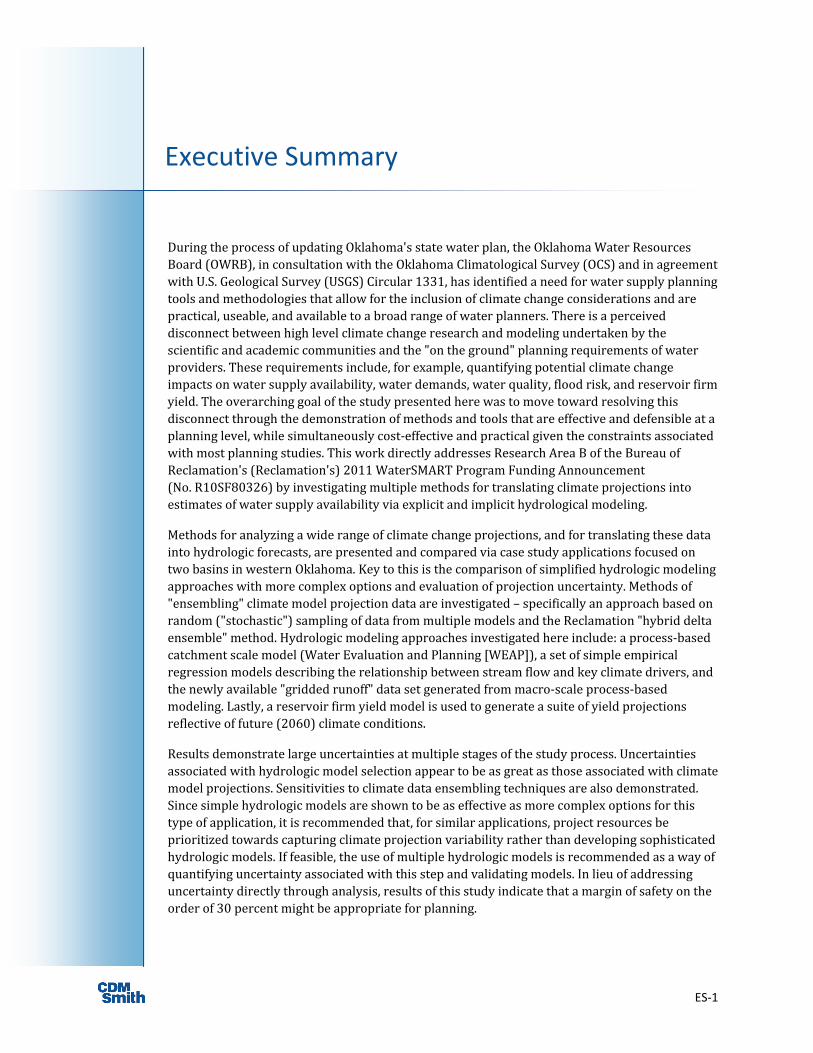
Executive Summary

During the process of updating Oklahoma's state water plan, the Oklahoma Water Resources Board (OWRB), in consultation with the Oklahoma Climatological Survey (OCS) and in agreement with U.S. Geological Survey (USGS) Circular 1331, has identified a need for water supply planning tools and methodologies that allow for the inclusion of climate change considerations and are practical, useable, and available to a broad range of water planners. There is a perceived disconnect between high level climate change research and modeling undertaken by the scientific and academic communities and the "on the ground" planning requirements of water providers. These requirements include, for example, quantifying potential climate change impacts on water supply availability, water demands, water quality, flood risk, and reservoir firm yield. The overarching goal of the study presented here was to move toward resolving this disconnect through the demonstration of methods and tools that are effective and defensible at a planning level, while simultaneously cost‐effective and practical given the constraints associated with most planning studies. This work directly addresses Research Area B of the Bureau of Reclamation's (Reclamation's) 2011 WaterSMART Program Funding Announcement (No. R10SF80326) by investigating multiple methods for translating climate projections into estimates of water supply availability via explicit and implicit hydrological modeling.

Methods for analyzing a wide range of climate change projections, and for translating these data into hydrologic forecasts, are presented and compared via case study applications focused on two basins in western Oklahoma. Key to this is the comparison of simplified hydrologic modeling approaches with more complex options and evaluation of projection uncertainty. Methods of "ensembling" climate model projection data are investigated – specifically an approach based on random ("stochastic") sampling of data from multiple models and the Reclamation "hybrid delta ensemble" method. Hydrologic modeling approaches investigated here include: a process‐based catchment scale model (Water Evaluation and Planning [WEAP]), a set of simple empirical regression models describing the relationship between stream flow and key climate drivers, and the newly available "gridded runoff" data set generated from macro‐scale process‐based modeling. Lastly, a reservoir firm yield model is used to generate a suite of yield projections reflective of future (2060) climate conditions.

Results demonstrate large uncertainties at multiple stages of the study process. Uncertainties associated with hydrologic model selection appear to be as great as those associated with climate model projections. Sensitivities to climate data ensembling techniques are also demonstrated. Since simple hydrologic models are shown to be as effective as more complex options for this type of application, it is recommended that, for similar applications, project resources be prioritized towards capturing climate projection variability rather than developing sophisticated hydrologic models. If feasible, the use of multiple hydrologic models is recommended as a way of quantifying uncertainty associated with this step and validating models. In lieu of addressing uncertainty directly through analysis, results of this study indicate that a margin of safety on the order of 30 percent might be appropriate for planning.

Executive Summary

ES‐2

Lastly, results demonstrate significant potential impacts of climate change on surface water yields in western Oklahoma. These arise from a combination of projected reductions in precipitation, changes in annual sequencing of precipitation (e.g., extended droughts), and increased evaporation and evapotranspiration (ET) due to temperature increases. Water resources practitioners are encouraged to consider these impacts in planning studies.

1‐1

Climate change science is evolving and becoming more accessible for water resources planning. For example, modeling projections of both future climate (precipitation [P]and temperature [T]) and surface runoff, representing 116 different sets of climate model projections, are now readily available for public download (http://gdo‐dcp.ucllnl.org/downscaled_cmip3_projections). These data have been downscaled to a useable spatial resolution for water resources planning studies (1/8° degree grid, 8 miles by 8 miles). They have also undergone "bias correction" to achieve acceptable reproduction of historical climate data and lend confidence to the predictions of the future. The data set represents a highly valuable contribution to the water resources planning community. However, challenging questions persist with respect to how best to use these data for water resources planning. There is a risk of under‐using the available data and modeling options and poorly informing decisionmaking due to scope limitations. There is also a risk of getting "lost" in the spectrum of available data and not generating useful results. These risks are primarily attributable to the large volume of model output now available and the uncertainty associated with these output – as demonstrated by the range of values projected. Methods that are both practical and defensible are therefore required for incorporating climate change science into water resources planning studies and for addressing the uncertainties in the analysis.

1.1 Modeling Uncertainty Multiple potential sources of uncertainty exist in climate change studies for water resources. The first major source of uncertainty is that directly attributable to differences in the global climate models (GCMs) used to develop the projections described above. These differences include differences in model construction, parameterization, and underlying assumptions. As stated in Brown (2011), "There are many sources of uncertainty that affect the projections, including uncertainty in the response of the Earth's climate system to greenhouse gas emissions, errors in the ways the models represent the Earth's climate system, and the unknown greenhouse gas emissions of the future. In some cases, the differences between projections from different models are so wide that planning for one climate projection would contradict planning for another."

A second major source of uncertainty in these types of studies is the modeling used to translate climate projections into the hydrologic parameters required for planning models (Xu et al. 2011; Prudhomme et al. 2009; Minville et al. 2008). Hydrologic modeling is subject to the same types of uncertainty identified for the climate models, resulting from basic model construction and underlying mathematical equations and assumptions and from model parameterization. No model is perfect in its numerical representation of complex natural processes; there is error in every prediction. The magnitude of this error is unknown – thus the uncertainty. We can reduce model uncertainty, and increase our confidence in model predictions, through calibration and verification exercises using measured data. Knowing that a model performs well in reproducing the past gives us some level of confidence in our predictions of the future.

Section 1 Introduction


1‐2

This is particularly true if the range of future conditions do not deviate significantly from the range contained in the calibration period. An important complication for climate change studies, however, is that this is often not the case. For example, a 50‐year historical record of climate data is unlikely to include the extent of high temperatures, nor possibly the extreme precipitation fluctuations, predicted by the climate models. The confidence added through calibration is therefore less compared to other types of studies.

Addressing uncertainty is a critical component to any climate change study. A recently published U.S. Environmental Protection Agency (EPA) handbook (CDM Smith 2011) suggests two general approaches for quantifying uncertainty in climate change impact studies: scenario planning and probabilistic methods. Scenario planning involves multiple model applications using discrete climate change scenarios, preferably spanning a range of climate forecasts (e.g., Xu et al. 2011; Cullis et al. 2011). Probabilistic methods involve fitting probability distributions to uncertain climate variables, likely using a large range of climate model projections. Generally some type of random sampling of these input distributions would be applied to generate probabilistic output (e.g., Manning et al. 2009; Ghosh and Mujumdar 2007; Wilby and Harris 2006). It should be noted that, since model predictions rather than observations are used, these types of output represent levels of consensus among the sampled models rather than true probabilities of occurrence. However, measures of model consensus are useful for assessing relative uncertainty levels. Although difficult to confirm, we presume that greater agreement among models is indicative of lower uncertainty in the predictions. With either probabilistic methods or scenario planning, final results are presented as a range of values, reflecting analysis uncertainty rather than a single deterministic value.

As part of either scenario planning or probabilistic methods, "ensembling" of climate projections is a popular approach for addressing uncertainties in GCM projections (Reclamation 2010; Manning et al. 2009). Ensembling involves the combining of GCM data sets into a single set that reflects the predictions of multiple GCMs. The ensemble data set is then used in subsequent analyses. There appears to be consensus in the literature that selecting a single "best" climate projection is challenging, if not impossible. Consequently, the use of multiple climate model projections in planning studies is recommended over relying on a single projection.

Reclamation (2010) previously investigated uncertainty associated with three combinations of ensemble‐hydrologic modeling approaches: delta method, hybrid‐delta method, and ensemble hybrid‐delta method. This Oklahoma‐specific study quantified significant differences in projections of both runoff and ET across the three methods.

1.2 Hydrologic Models A variety of hydrologic models, with a range of complexity and sophistication, have been applied in the literature for translating climate change projections into flow projections. These include mechanistic models, where the key physical processes are explicitly represented in the model (e.g., Gosling et al. 2011; Traynham et al. 2011; Minville et al. 2008) and empirical models where the processes are implicit in the model (e.g., Nilsson et al. 2008; Stewart et al. 2004; Duell 1994). These also include both macro‐scale models without site‐specific calibration (e.g., Maurer et al. 2010; Maurer 2007) and models that are locally calibrated and applied (e.g., Yates et al. 2009; Groves et al. 2008). The studies of Gosling et al. (2011) and Maurer et al. (2010) assessed the importance of hydrologic model selection in climate change studies. Both studies concluded that the uncertainty associated with hydrologic model selection is secondary compared to climate model uncertainty with respect to predicting changes in mean annual flow. However, both studies also showed a greater sensitivity to the selection of hydrologic models when the models are used for simulating low flows. Presumably, this result is particularly significant for studies focused on water supply gaps or firm yields where low flows are critical.


1‐3

A 2011 study for the State of Oklahoma (AMEC 2011) quantified streamflow sensitivity to climate change at a statewide scale. This study used the Reclamation "hybrid delta ensemble" method (Reclamation 2010) to modify historical flow records based on projections of future changes in runoff using a suite of GCM projections and a macro‐scale hydrologic model. The hydrologic model was essentially uncalibrated at a local scale. Results of this study indicate potential changes in annual streamflow ranging from 60 percent to 140 percent of historical levels, depending on location and choice of ensembled GCM output, for a 2060 planning horizon. For the Foss Reservoir watershed, this study quantified changes in annual streamflow of ‐32 percent, ‐9 percent, and +18 percent for the worst case, central tendency, and best case ensemble scenarios, respectively. For the Lugert Altus Reservoir watershed, changes of ‐34 percent, ‐13 percent, and +15 percent were quantified for the three scenarios.

1.3 Firm Yield The analysis described above was used in combination with projected changes in water demand to support forecasts of potential water supply gaps across Oklahoma. At a local level, reservoir firm yield calculations often feature in planning studies as a means of quantifying future dependable supply availability. Firm yield is typically defined as the maximum annual demand that can be fully met with reservoir withdrawals throughout the period of analysis, including critical drought conditions. For water providers dependent on stored surface water, firm yield is a critical component of their planning. It is a calculated, rather than measured, value and is dependent on anticipated available source water flow, the storage capacity of the reservoir, reservoir evaporation and other losses, direct precipitation, reservoir operational constraints (if applicable), and the seasonal pattern of water demands placed on the reservoir. Firm yield is sensitive to climate variability indirectly through both the pattern and magnitude of reservoir inflows and net evaporative losses.

1.4 Study Goals The primary goal of the study presented here was to demonstrate and compare practical methods for incorporating climate change into water resources planning studies. While the focus of this particular study is on reservoir firm yield projections, the methods and tools are equally relevant for any water resources planning study that relies on surface hydrology data at a monthly timescale. Investigating uncertainty in both climate and hydrologic modeling projections was also key to the study. Specifically, through case study applications, we aimed to:

Compare methods for addressing climate model uncertainty through ensembling and climate data processing techniques;

Compare hydrologic modeling options ranging in complexity from low to moderate;

Assess sensitivities to assumed greenhouse gas emission scenarios through inclusion of two differing emission pathway scenarios (A2 and B1);

Demonstrate two new tools, developed as part of this study, designed to provide for automated climate data processing and enhanced reservoir firm yield analysis with allowance for climate change; and

Quantify locally‐relevant stream flow and reservoir firm yield sensitivities to climate change projections, by presenting ranges of final output, for two case study reservoirs in western Oklahoma and a 2060 projection horizon.

2‐1

Section 2 Case Study Site Locations

Foss and Lugert‐Altus Reservoirs in western Oklahoma were selected as case study sites for this study (Figure 1). Key features of each are summarized in Table 1. Both sites were appealing due to their availability of required data (Table 1 and Table 2), including existing Reclamation firm yield studies, and the lack of major upstream storage or point diversions. The difference in primary water use (municipal and industrial [M&I] vs. agricultural) results in different seasonal reservoir demand patterns, a key feature of firm yield studies. This makes for an interesting comparative analysis. In short, the two basins satisfied certain minimum criteria, were similar enough (e.g., geographic location, upstream water use) to provide for a level of duplication and confirmation of methods, while still different in catchment size and seasonal demand patterns to provide for a comparative analysis.

Water users in the Foss Reservoir catchment rely on a combination of surface water and alluvial groundwater to meet roughly 40 percent of existing demands, with the remainder met with deep (bedrock) groundwater. Water demands in the basin are projected to increase by approximately 40 percent by 2060. The majority of this increased demand is projected to come from the oil and gas sector. For the Lugert‐Altus Reservoir catchment, the vast majority of current demands are met through surface water and alluvial groundwater supplies. These demands are projected to increase to approximately 70 percent by 2060, with frequent future shortfalls projected based on existing supplies. For more information on both basins, the reader is referred to the recently completed update to the Oklahoma Comprehensive Water Plan (OCWP) (CDM Smith 2011b).

Section 2 Case Study Site Locations

2‐2

Figure 1: Case Study Catchments

Table 1: Summary Case Study Reservoirs

Reservoir Catchment Size (Mi2)

Catchment Land Cover

Conservation Pool Capacity

(AF)

Primary Reservoir Water

Supply Use

Reservoir Surface Area At Capacity

(Acre)

Existing Published Firm Yield (AFY)1

Foss 1,500 63% grassland; 24% scrub; 8% crop; 2% developed

177,000 M&I 9,000 18,000

Lugert‐Altus

2,800 55% grassland; 21% scrub; 17% crop; 3% developed

111,000 agriculture 6,000 47,000

1 CDM Smith 2011b Mi2 square miles AF acre‐feet AFY acre‐feet per year

Table 2: Summary of Upstream Flow Gages

Gage Description Drainage Area

(Mi2) Period Of Record Mean Annual Flow

(AFY)

USGS 7324200 (Foss) Washita River near Hammon 1,400 1969 – present 47,000

USGS 7301500 (Lugert‐Altus)

N. Fork Red River near Carter 2,300 1944 ‐ present 90,000

3‐1

Section 3 Methods

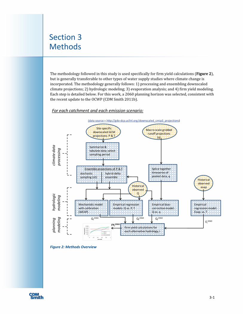
The methodology followed in this study is used specifically for firm yield calculations (Figure 2), but is generally transferable to other types of water supply studies where climate change is incorporated. The methodology generally follows: 1) processing and ensembling downscaled climate projections; 2) hydrologic modeling; 3) evaporation analysis; and 4) firm yield modeling. Each step is detailed below. For this work, a 2060 planning horizon was selected, consistent with the recent update to the OCWP (CDM Smith 2011b).

Figure 2: Methods Overview

Site‐specific downscaled GCM projections: P & T

For each catchment and each emission scenario:

(data source = http://gdo‐dcp.ucllnl.org/downscaled_cmip3_projections)

Macro‐scale gridded runoff projections

(q)

Summarize & tabulate data; select sampling period

Splice together timeseries of pooled data, q

Ensemble projections of P & T

stochastic sampling (x5)

hybrid‐delta ensemble

Historical observed

Q

Mechanistic model with calibration (WEAP)

Empirical regression models: Q vs. P, T

Empirical bias‐correction model: Q vs. q

Historical observed evap

Empirical regression model: Evap. vs. T

Firm yield calculations for each alternative hydrology, i

Qi2060 Qi

2060 Qi2060

Ei2060

clim

ate data

processing

hydrologic

modeling

planning

modeling

0

5,000

10,000

15,000

20,000

25,000

0 0.2 0.4 0.6 0.8 1

firm

yield (A

FY)

percentile

2060 A2

2060 B1

historical baseline

FYi2060

Section 3 Methods

3‐2

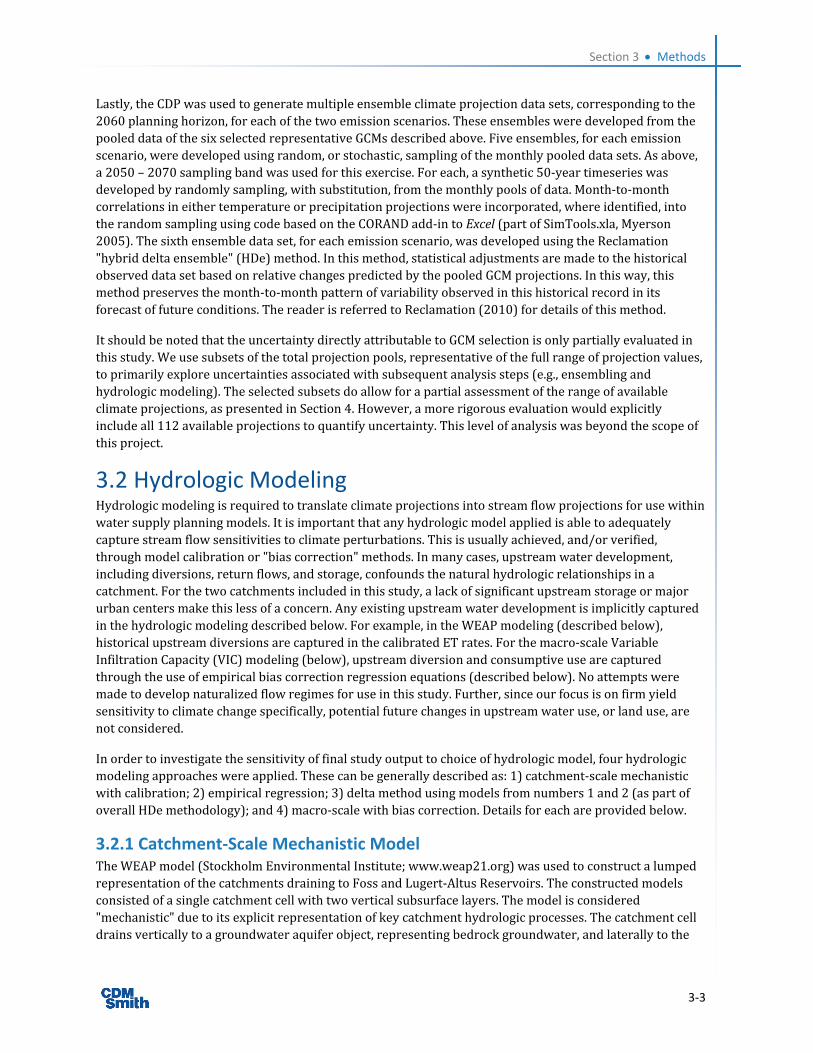
3.1 Climate Data Processing Six sets of downscaled GCM projections, developed by six different global research institutes, were used in this study for each of two greenhouse gas emission scenarios (Table 3). The data were downloaded from the Reclamation website (http://gdo‐dcp.ucllnl.org/downscaled_cmip3_projections), described in Maurer et al. (2007). Emission scenarios included in this study correspond to the A2 and B1 scenarios of the IPCC Special Report on Emission Scenarios (SRES). These scenarios are described, respectively, as: "A2 (~"higher" emissions path) technological change and economic growth more fragmented, slower, higher population growth; and "B1 (~"lower" emissions path) rapid change in economic structures toward service and information, with emphasis on clean, sustainable technology. Reduced material intensity and improved social equity." Data were obtained for all cells included in the overlap of the 1/8° grid and the reservoir catchments (Figure 1).

Table 3: Summary of Selected GCMs

GCMs Green House Emission Scenarios

Bjerknes Centre for Climate Research's Model (bccr_bcm2_0.1)

SRES Scenarios A2, B1

Meteorological Research Institute, Japan (mri_cgcm2_3_2a.1)

Geophysical Fluid Dynamics Laboratory (GFDL) Coupled Model, USA (gfdl_cm2_0.1)

CSIRO Atmospheric Research, Australia (csiro_mk3_0.1)

National Center for Atmospheric Research, Community Climate System Model, USA (ncar_ccsm3_0.1)

Max Planck Institute for Meteorology, Germany (mpi_echam5.1)

The GCMs were selected based on a previous analysis for Oklahoma (AMEC 2011), which ordered each of the 112 available GCM projections into one of four quartiles representing: hot/dry, hot/wet, warm/dry, and warm/wet conditions, respectively. This ordering was based on statewide annual average deviations in 2060 temperature and precipitation projections compared to baseline historical means. Additionally, an overlapping inner‐quartile range was defined, representing a central tendency subset. For our study, a single GCM projection from each of the four quartiles developed for the A2 scenario, and two from the central tendency set, were selected to provide a reasonable representation of the range of GCM projections available (Table 3).

In addition to the model projections of future climate described above, a set of historical observed temperature and precipitation data, for the period 1950 – 1999, were downloaded from the source cited above. These data have been projected onto the same 1/8° grid as the climate model projections, using historical weather station data. Maurer et al. (2007) provides details on the techniques used to generate this data set.

A new tool was developed under this study designed to facilitate the processing of downscaled GCM projection data. The Climate Data Processor (CDP) is a Microsoft Excel‐based tool with customized Visual Basic code. The CDP provides automated graphical and tabular summaries of large volumes of projection data to allow for easy comparisons of model projections and visualization of forecast climate trends. It also provides multiple automated options for data ensembling. The CDP was first used to calculate area‐weighted mean monthly timeseries for each of the 12 selected projections. Weightings were based on the percent overlap of grid and catchment area, for the two catchments respectively, as calculated in geographic information system (GIS). Secondly, the CDP was used to generate graphical and tabular summaries of the selected climate data relevant to the 2060 planning horizon. For this task, and for use in all others described below, a sampling band of 10 years around the planning target was applied (i.e., 2060 + 10 years).

Section 3 Methods

3‐3

Lastly, the CDP was used to generate multiple ensemble climate projection data sets, corresponding to the 2060 planning horizon, for each of the two emission scenarios. These ensembles were developed from the pooled data of the six selected representative GCMs described above. Five ensembles, for each emission scenario, were developed using random, or stochastic, sampling of the monthly pooled data sets. As above, a 2050 – 2070 sampling band was used for this exercise. For each, a synthetic 50‐year timeseries was developed by randomly sampling, with substitution, from the monthly pools of data. Month‐to‐month correlations in either temperature or precipitation projections were incorporated, where identified, into the random sampling using code based on the CORAND add‐in to Excel (part of SimTools.xla, Myerson 2005). The sixth ensemble data set, for each emission scenario, was developed using the Reclamation "hybrid delta ensemble" (HDe) method. In this method, statistical adjustments are made to the historical observed data set based on relative changes predicted by the pooled GCM projections. In this way, this method preserves the month‐to‐month pattern of variability observed in this historical record in its forecast of future conditions. The reader is referred to Reclamation (2010) for details of this method.

It should be noted that the uncertainty directly attributable to GCM selection is only partially evaluated in this study. We use subsets of the total projection pools, representative of the full range of projection values, to primarily explore uncertainties associated with subsequent analysis steps (e.g., ensembling and hydrologic modeling). The selected subsets do allow for a partial assessment of the range of available climate projections, as presented in Section 4. However, a more rigorous evaluation would explicitly include all 112 available projections to quantify uncertainty. This level of analysis was beyond the scope of this project.

3.2 Hydrologic Modeling Hydrologic modeling is required to translate climate projections into stream flow projections for use within water supply planning models. It is important that any hydrologic model applied is able to adequately capture stream flow sensitivities to climate perturbations. This is usually achieved, and/or verified, through model calibration or "bias correction" methods. In many cases, upstream water development, including diversions, return flows, and storage, confounds the natural hydrologic relationships in a catchment. For the two catchments included in this study, a lack of significant upstream storage or major urban centers make this less of a concern. Any existing upstream water development is implicitly captured in the hydrologic modeling described below. For example, in the WEAP modeling (described below), historical upstream diversions are captured in the calibrated ET rates. For the macro‐scale Variable Infiltration Capacity (VIC) modeling (below), upstream diversion and consumptive use are captured through the use of empirical bias correction regression equations (described below). No attempts were made to develop naturalized flow regimes for use in this study. Further, since our focus is on firm yield sensitivity to climate change specifically, potential future changes in upstream water use, or land use, are not considered.

In order to investigate the sensitivity of final study output to choice of hydrologic model, four hydrologic modeling approaches were applied. These can be generally described as: 1) catchment‐scale mechanistic with calibration; 2) empirical regression; 3) delta method using models from numbers 1 and 2 (as part of overall HDe methodology); and 4) macro‐scale with bias correction. Details for each are provided below.

3.2.1 Catchment‐Scale Mechanistic Model The WEAP model (Stockholm Environmental Institute; www.weap21.org) was used to construct a lumped representation of the catchments draining to Foss and Lugert‐Altus Reservoirs. The constructed models consisted of a single catchment cell with two vertical subsurface layers. The model is considered "mechanistic" due to its explicit representation of key catchment hydrologic processes. The catchment cell drains vertically to a groundwater aquifer object, representing bedrock groundwater, and laterally to the

Section 3 Methods

3‐4

stream network. Monthly stream flows are calculated using the model's "soil moisture method," in which net precipitation infiltrates to an upper shallow zone, accumulates as snow pack, or flows laterally as direct runoff. Water is stored in both vertical layers, with downward infiltration from the top layer to the bottom layer as parameterized by a vertical conductivity coefficient. ET losses are from the top layer only and calculated in the model as a function of vegetation‐specific potential ET parameters and storage level in the top layer. Water leaves the two subsurface layers, contributing to stream baseflow, as a function of storage levels and lateral conductivity coefficients.

WEAP models for Foss and Lugert‐Altus Reservoir catchments were calibrated based on 50‐year (1950 – 1999) records of measured stream flows from the USGS gages listed in Table 2 and shown in Figure 1. For gage 07324200 (Washita), USGS records were supplemented with estimated reservoir inflow calculations and local stream gaging records for the period prior to 1969. Climate input data for the calibration period were taken from the gridded historical set described above, averaged over the catchment areas. Model calibration focused on selected key input parameters: snow melt and freeze temperatures (Tmelt and Tfreeze), vertical and horizontal subsurface hydraulic conductivities, subsurface storage capacities, and surface PET coefficients. The calibration relied on manual trial and error of parameter values, within realistic ranges, to minimize the total root mean squared error (RMSE) between measured and modeled monthly flows. An accurate flow balance was also targeted as part of the calibration process (i.e., matching total flow and achieving realistic distributions of stream flow vs. ET losses vs. groundwater infiltration). Stationarity is assumed for the historical data such that a single set of model internal parameters are used to simulate the full historical period (only climate inputs vary). The calibrated models were then used to simulate 2060 hydrologic conditions using the various sets of 2060 climate data described in Section 3.1. Again, this assumes stationarity for all but the climate parameters.

As a model verification exercise, a split sample cross‐validation was performed using the calibrated Lugert‐Altus model and a 12‐year period preceding the calibration period: 1938 – 1949. Gaged flow data for this period were available to test the model's effectiveness at simulating flows outside of the calibration period. Climate data for this period were obtained from the Elk City weather station (Figure 1). Linear regression models (not shown), developed using the gridded historical climate data set, were used to translate Elk City climate (grid cell 164, Figure 1) to catchment average climate. Model parameters were maintained at calibrated values. Adequate gaged flow data were not available for the Foss catchment and therefore a similar exercise could not be performed for the Foss catchment models.

3.2.2 Empirical Regression Models As a second hydrologic modeling approach, statistically significant (P < 0.1) empirical regression models were developed for each catchment that describe the relationship between monthly stream flow and climate variables (P and T) using simple fitted equations. Models were developed for each calendar month using gridded historical climate data (1950 – 1999) and observed monthly flow data. Regression analyses were performed within Microsoft Excel. This analysis involved ordered iterative changes to climate predictor variables, starting with 1‐month and increasing to 12‐month cumulative values, until we were satisfied that the optimal set (highest coefficient of determination [R2]) had been found.

As above, a split sample cross‐validation exercise was performed using the empirical regression models and the 1938 – 1949 data record. The methods were the same as described above. Also as above, the assumption of parameter stationarity is key to this approach.

Section 3 Methods

3‐5

3.2.3 Delta Method In the third approach, both sets of models described above were applied within the HDe methodology (see Reclamation 2010). The models were applied using the 2060 HDe climate projections. As described in Section 3.1, these climate projections were developed by adjusting the 1950 – 1999 historical record to reflect ensemble forecasts of the 2060 planning horizon. In keeping with this approach, the 50‐year flow record, corresponding to the same period, was adjusted based on the difference between flows modeled using the 2060 HDe climate projections and the flows modeled using the historical observed climate data set. This can be written as:

∆ (1)

∆ (2)

where Qt2060 = final adjusted monthly flow record reflecting 2060 climate conditions, Qtobs = historical observed flow record (1950 – 1999), QtHDe = modeled flows using 2060 HDe climate projections, Qtbase = modeled historical flows (1950 – 1999), and t = monthly index for the 50‐year period.

3.2.4 Macro‐Scale with Bias Correction Reclamation recently published a new data set of climate change hydrologic projections. These projections cover the period 2000 – 2100 and were generated using the full suite of downscaled GCM output available from the Reclamation website and a macro‐scale hydrologic model ("Variable Infiltration Capacity" or "VIC" model). Hydrologic model output, including monthly surface runoff values, are available for the western United States and are projected onto the same 1/8° grid as the downscaled climate data. We term the surface runoff output "gridded runoff" for the purposes of this paper. The VIC model is not locally calibrated, nor does it include groundwater interactions. Further details of the model and parameterization of the model are provided elsewhere (Reclamation 2011).

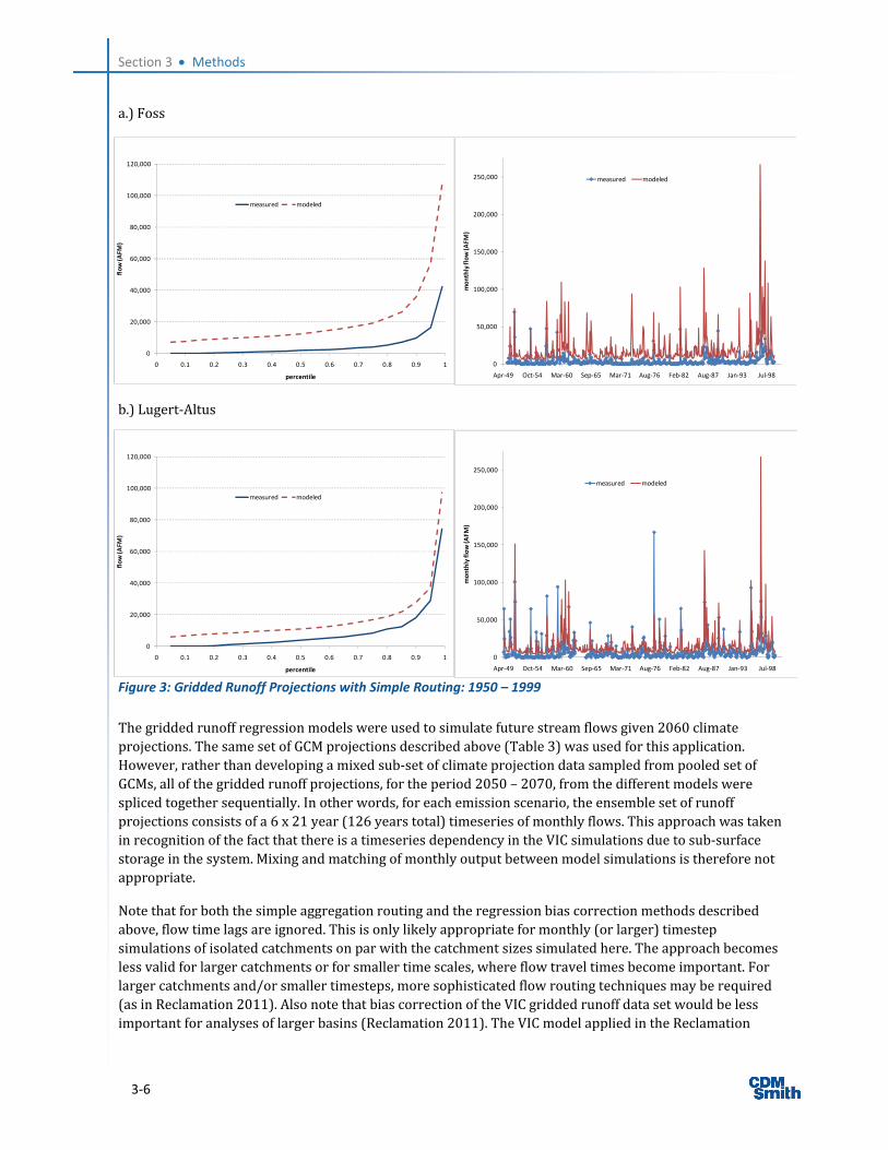
A goal of this study was to investigate the use of this new data set within a catchment scale planning study. Therefore, as a fourth hydrologic modeling option, gridded runoff projections were used to simulate stream flow in our case study basins. The modeled historical period (1950 – 1999) was used to assess the validity of directly using the gridded runoff data set in stream flow simulations. As a first option, simple routing of the gridded runoff was applied. In this approach, all grid cell runoff values contained in the respective catchments were summed, with appropriate weightings applied for partial grid cells. It was immediately clear that this approach, while generally capturing the pattern of variability in the monthly flows, grossly overestimated the magnitudes of the flows (Figure 3). It was therefore deemed an invalid option for our purposes. Instead, the identified bias was addressed by developing simple monthly regression models describing the relationship between measured stream flow and modeled gridded runoff. These models, analogous to the empirical regression models described above, were developed using the 1950 – 1999 historical record of gaged flow data and catchment‐averaged gridded runoff projections for the same period.

Section 3 Methods

3‐6

a.) Foss

b.) Lugert‐Altus

Figure 3: Gridded Runoff Projections with Simple Routing: 1950 – 1999

The gridded runoff regression models were used to simulate future stream flows given 2060 climate projections. The same set of GCM projections described above (Table 3) was used for this application. However, rather than developing a mixed sub‐set of climate projection data sampled from pooled set of GCMs, all of the gridded runoff projections, for the period 2050 – 2070, from the different models were spliced together sequentially. In other words, for each emission scenario, the ensemble set of runoff projections consists of a 6 x 21 year (126 years total) timeseries of monthly flows. This approach was taken in recognition of the fact that there is a timeseries dependency in the VIC simulations due to sub‐surface storage in the system. Mixing and matching of monthly output between model simulations is therefore not appropriate.

Note that for both the simple aggregation routing and the regression bias correction methods described above, flow time lags are ignored. This is only likely appropriate for monthly (or larger) timestep simulations of isolated catchments on par with the catchment sizes simulated here. The approach becomes less valid for larger catchments or for smaller time scales, where flow travel times become important. For larger catchments and/or smaller timesteps, more sophisticated flow routing techniques may be required (as in Reclamation 2011). Also note that bias correction of the VIC gridded runoff data set would be less important for analyses of larger basins (Reclamation 2011). The VIC model applied in the Reclamation

0

20,000

40,000

60,000

80,000

100,000

120,000

0 0.1 0.2 0.3 0.4 0.5 0.6 0.7 0.8 0.9 1

flow (A

FM)

percentile

measured modeled

0

20,000

40,000

60,000

80,000

100,000

120,000

0 0.1 0.2 0.3 0.4 0.5 0.6 0.7 0.8 0.9 1

flow (A

FM)

percentile

measured modeled

0

50,000

100,000

150,000

200,000

250,000

Apr‐49 Oct‐54 Mar‐60 Sep‐65 Mar‐71 Aug‐76 Feb‐82 Aug‐87 Jan‐93 Jul‐98

monthly flow (A

FM)

measured modeled

0

50,000

100,000

150,000

200,000

250,000

Apr‐49 Oct‐54 Mar‐60 Sep‐65 Mar‐71 Aug‐76 Feb‐82 Aug‐87 Jan‐93 Jul‐98

monthly flow (A

FM)

measured modeled

Section 3 Methods

3‐7

(2011) study was calibrated on a large spatial scale and differences in catchment hydrologic parameters are likely smoothed out as scales are increased.

The regression‐based bias correction method presented here is new and differs from the approach presented in the 2011 Reclamation study. The Reclamation method involves "quantile mapping" whereby projected monthly values are adjusted based on the value's relative percentile within the full range of projection values for that given month. The percentile value is used to identify an adjustment factor calculated using the measured vs. modeled "overlap period" data set (1950 – 1999). Seemingly, a potential weakness in this approach is its handling of projected flow rates that fall outside of the range simulated for the overlap period. In this situation, the adjustment factor associated with the maximum (or minimum) percentiles of the overlap period is used. This amounts to linear extrapolation using only the maximum percentile points. The monthly regression approach featured in this study is presented as a potential, and likely simpler and more transparent, alternative to the quantile mapping technique. It also appears to better handle extreme events (flows outside of the historical overlap period) by using a regression curve, not constrained to linear, fitted to the full range of historical data. However, an in‐depth comparison of the two bias correction techniques is outside the scope of this study.

3.3 Evaporation Analysis To allow for the simulation of future changes in reservoir evaporation rate due to climate change, relationships between evaporation rates and mean monthly temperature were quantified. Empirical regression models were developed for each reservoir using historical measured pan evaporation and temperature data. A single model was developed for each reservoir describing the relationship between reservoir surface evaporation and monthly temperature at the reservoir. A pan coefficient of 0.7 was applied to measured pan evaporation rates to convert to reservoir surface rates. To facilitate use of the catchment averaged climate data described above, relationships between reservoir‐specific climate (air temperature and precipitation) and catchment average values were also quantified with linear regression equations based on historical data. The developed evaporation models were then used in conjunction with the 2060 climate projections to project a monthly timeseries of reservoir evaporation rates corresponding to each of the ensemble climate projections described above. These gross evaporation rates were converted to net evaporation, for use in the firm yield models, by subtracting out monthly precipitation values. Net monthly evaporation rates (in mo‐1) are converted to total evaporation losses (AFM) within the Reservoir Yield Model (described below) by multiplying by reservoir surface area. Surface areas are estimated within the model based on calculated reservoir storage volumes and user‐defined area‐volume tables.

As with hydrologic modeling, multiple published options exist for physically‐based mechanistic modeling of evaporation. However, the approach presented here represents an appealing practical option for isolating the relationship between evaporation rates and climate on a site‐specific basis.

3.4 Firm Yield Modeling CDM Smith's Reservoir Yield Model was used to calculate firm yields for the suite of hydrologic projections. The Reservoir Yield Model is a generalized water allocation model, housed in Microsoft Excel, which includes an automated firm yield calculator. The firm yield calculations are performed in the model through iterative increases in annual demand until the reservoir available conservation pool is emptied at some point in the period of simulation. The model can accommodate multiple alternative inflow hydrologic data sets. Output can be provided as probabilistic plots of calculated firm yield values, displaying the range of calculated values and levels of consensus among the different data sets. The model was verified against other similar tools, including Reclamation's Reservoir Operations Model, in a separate study for the State of Oklahoma (CDM Smith 2009).

Section 3 Methods

3‐8

Monthly demand patterns were assumed based on previous Reclamation firm yield analyses for the two reservoirs. These monthly distributions of annual demand assume predominant M&I usage for Foss and agricultural usage for Lugert Altus (Table 4). Net evaporation rates for each simulated scenario were calculated externally (Section 3.3) and input to the model as a monthly timeseries.

Table 4: Monthly Demand Distributions (%) Assumed in Firm Yield Modeling

Jan Feb Mar Apr May Jun Jul Aug Sep Oct Nov Dec

Foss 4 4 4 6 10 13 16 15 12 8 4 4

Lugert‐Altus

0 0 0 0 4 6 41.5 41.5 7 0 0 0

The model was applied to each of the alternative monthly inflow data sets, for each emission scenario and each catchment, consisting of: 5 x 50 years of WEAP output, 5 x 50 years of empirical regression output, 1 x 50 years of HDe WEAP output, 1 x 50 years of HDe empirical regression output, and 1 x 126 years of gridded runoff with bias correction output.

4‐1

Section 4 Results

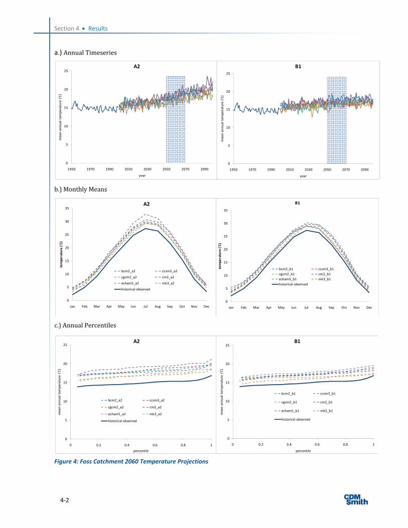
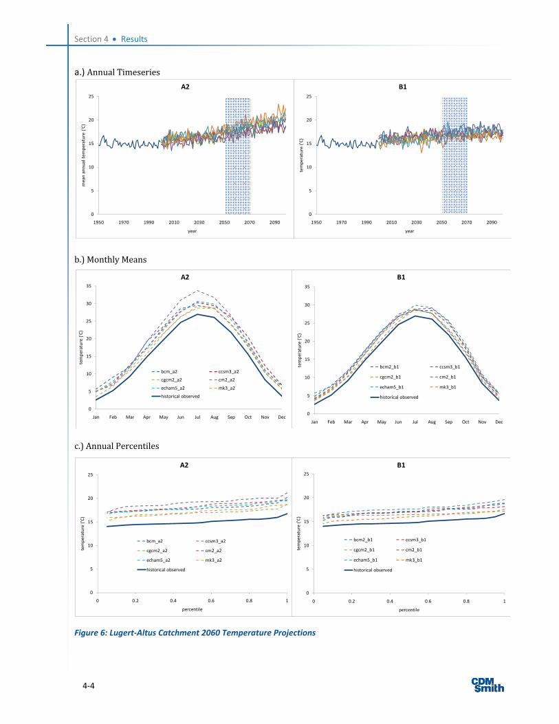
4.1 Climate Projections Catchment‐averaged annual T projections show an increase of approximately 4 and 2 degrees Celsius (°C) through 2099 for the A2 and B1 emission scenarios, respectively (Figures 4a and 6a). For the 2060 planning horizon (highlighted on annual timeseries plots), median annual Ts are projected to increase by approximately 3 (±1) and 2 (±1) °C, for the two emission scenarios, respectively (Figures 4c and 6c). Seasonal patterns of T are not projected to change (Figures 4b and 6b). Worst‐case projections show an increase in mean July T of up to 5°C (A2 scenario, GFDL cm2 model).

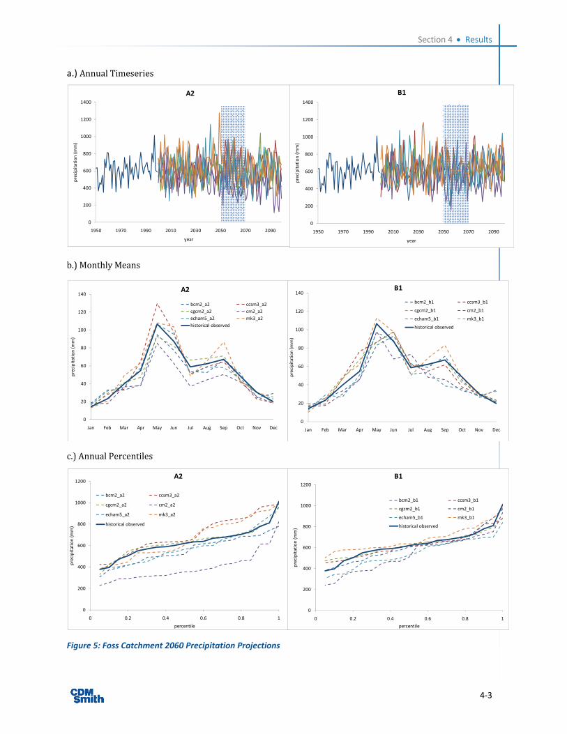
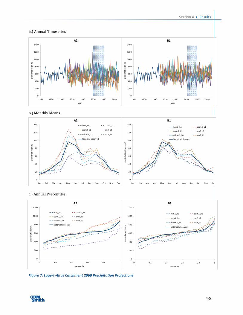
P projections display a broader band of uncertainty and lack clearly defined temporal trends (Figures 5a and 7a). Projections for the A2 emissions scenario generally show greater variability in annual P, with more extreme high and low annual P for the 2060 planning horizon, compared to the B1 scenario (Figures 5c and 7c). Seasonal patterns of P are not projected to change under either emission scenario (Figures 5b and 7b).

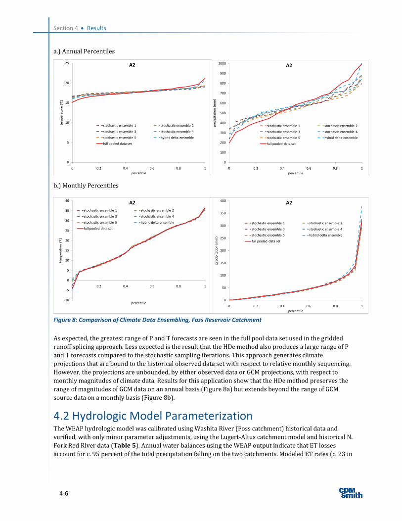
A comparison of ensemble data sets is presented in Figure 8 for the Foss Reservoir catchment and the A2 emissions scenario. The results for the B1 scenario and the Lugert‐Altus catchment are similar but not shown. Shown in this figure, for each emission scenario, are the five iterations of the stochastic ensembling method, the HDe method, and the full pool of climate model projection data. The latter was used by Reclamation (Reclamation 2011) to generate the gridded runoff data set used here (spliced together across the selected GCMs). Each of these data sets serve as inputs to the hydrologic and evaporation models described below. While preserving the general statistics of the pooled projections, the different ensembling techniques produce notably different results. This is particularly true for the precipitation ensembles. Variability in annual precipitation percentiles, across the seven ensembling methods, ranges from approximately 10 percent (middle percentiles) to 30 percent (lower and upper percentiles). In other words, the span of annual precipitation values at the low and high percentiles represent up to an approximately 30 percent difference ((max – min)/min). For example, at the 20 percentile level, we observe a range of approximately 100 mm (500 – 400), a 25 percent difference between the two extremes. Variability in annual mean temperature percentiles is less, ranging from 5 – 6 percent (±1°C) at the lower and upper percentiles down to < 1 percent (0.1°C) at the middle percentiles.

Section 4 Results

4‐2

a.) Annual Timeseries

b.) Monthly Means

c.) Annual Percentiles

Figure 4: Foss Catchment 2060 Temperature Projections

0

5

10

15

20

25

30

35


temperature ('C)

A2

bcm2_a2 ccsm3_a2

cgcm2_a2 cm2_a2

echam5_a2 mk3_a2

historical observed

0

5

10

15

20

25

30

35


temperature ('C)

B1

bcm2_b1 ccsm3_b1

cgcm2_b1 cm2_b1

echam5_b1 mk3_b1

historical observed

0

5

10

15

20

25

1950 1970 1990 2010 2030 2050 2070 2090

mean annual tem

perature ('C)

year

A2

0

5

10

15

20

25

1950 1970 1990 2010 2030 2050 2070 2090

mean annual tem

perature ('C)

year

B1

0

5

10

15

20

25

0 0.2 0.4 0.6 0.8 1

mean annual tem

perature ('C)

percentile

A2

bcm2_a2 ccsm3_a2

cgcm2_a2 cm2_a2

echam5_a2 mk3_a2

historical observed

0

5

10

15

20

25

0 0.2 0.4 0.6 0.8 1

mean annual tem

perature ('C)

percentile

B1

bcm2_b1 ccsm3_b1

cgcm2_b1 cm2_b1

echam5_b1 mk3_b1

historical observed

Section 4 Results

4‐3


b.) Monthly Means


Figure 5: Foss Catchment 2060 Precipitation Projections

0

20

40

60

80

100

120

140


precipitation (mm)

A2

bcm2_a2 ccsm3_a2

cgcm2_a2 cm2_a2

echam5_a2 mk3_a2

historical observed

0

20

40

60

80

100

120

140


precipitation (mm)B1

bcm2_b1 ccsm3_b1

cgcm2_b1 cm2_b1

echam5_b1 mk3_b1

historical observed

0

200

400

600

800

1000

1200

1400

1950 1970 1990 2010 2030 2050 2070 2090

precipitation (mm)

year

A2

0

200

400

600

800

1000

1200

1400

1950 1970 1990 2010 2030 2050 2070 2090

precipitation (mm)

year

B1

0

200

400

600

800

1000

1200

0 0.2 0.4 0.6 0.8 1

precipitation (mm)

percentile

A2

bcm2_a2 ccsm3_a2

cgcm2_a2 cm2_a2

echam5_a2 mk3_a2

historical observed

0

200

400

600

800

1000

1200

0 0.2 0.4 0.6 0.8 1

precipitation (mm)

percentile

B1

bcm2_b1 ccsm3_b1

cgcm2_b1 cm2_b1

echam5_b1 mk3_b1

historical observed

Section 4 Results

4‐4


b.) Monthly Means


Figure 6: Lugert‐Altus Catchment 2060 Temperature Projections

0

5

10

15

20

25

30

35


temperature ('C)

A2

bcm_a2 ccsm3_a2

cgcm2_a2 cm2_a2

echam5_a2 mk3_a2

historical observed

0

5

10

15

20

25

30

35


temperature ('C)

B1

bcm2_b1 ccsm3_b1

cgcm2_b1 cm2_b1

echam5_b1 mk3_b1

historical observed

0

5

10

15

20

25

1950 1970 1990 2010 2030 2050 2070 2090

mean annual tem

perature ('C)

year

A2

0

5

10

15

20

25

1950 1970 1990 2010 2030 2050 2070 2090

temperature ('C)

year

B1

0

5

10

15

20

25

0 0.2 0.4 0.6 0.8 1

temperature ('C)

percentile

A2

bcm_a2 ccsm3_a2

cgcm2_a2 cm2_a2

echam5_a2 mk3_a2

historical observed

0

5

10

15

20

25

0 0.2 0.4 0.6 0.8 1

temperature ('C)

percentile

B1

bcm2_b1 ccsm3_b1

cgcm2_b1 cm2_b1

echam5_b1 mk3_b1

historical observed

Section 4 Results

4‐5


b.) Monthly Means


Figure 7: Lugert‐Altus Catchment 2060 Precipitation Projections

0

20

40

60

80

100

120

140


precipitation (mm)

A2

bcm_a2 ccsm3_a2

cgcm2_a2 cm2_a2

echam5_a2 mk3_a2

historical observed

0

20

40

60

80

100

120

140


precipitation (mm/m

o)

B1

bcm2_b1 ccsm3_b1

cgcm2_b1 cm2_b1

echam5_b1 mk3_b1

historical observed

0

200

400

600

800

1000

1200

1400

1950 1970 1990 2010 2030 2050 2070 2090

precipitation (mm)

year

A2

0

200

400

600

800

1000

1200

1400

1950 1970 1990 2010 2030 2050 2070 2090

precipitation (mm)

year

B1

0

200

400

600

800

1000

1200

0 0.2 0.4 0.6 0.8 1

precipitation (mm)

percentile

A2

bcm_a2 ccsm3_a2

cgcm2_a2 cm2_a2

echam5_a2 mk3_a2

historical observed

0

200

400

600

800

1000

1200

0 0.2 0.4 0.6 0.8 1

precipitation (mm)

percentile

B1

bcm2_b1 ccsm3_b1

cgcm2_b1 cm2_b1

echam5_b1 mk3_b1

historical observed

Section 4 Results

4‐6

a.) Annual Percentiles

b.) Monthly Percentiles

Figure 8: Comparison of Climate Data Ensembling, Foss Reservoir Catchment

As expected, the greatest range of P and T forecasts are seen in the full pool data set used in the gridded runoff splicing approach. Less expected is the result that the HDe method also produces a large range of P and T forecasts compared to the stochastic sampling iterations. This approach generates climate projections that are bound to the historical observed data set with respect to relative monthly sequencing. However, the projections are unbounded, by either observed data or GCM projections, with respect to monthly magnitudes of climate data. Results for this application show that the HDe method preserves the range of magnitudes of GCM data on an annual basis (Figure 8a) but extends beyond the range of GCM source data on a monthly basis (Figure 8b).

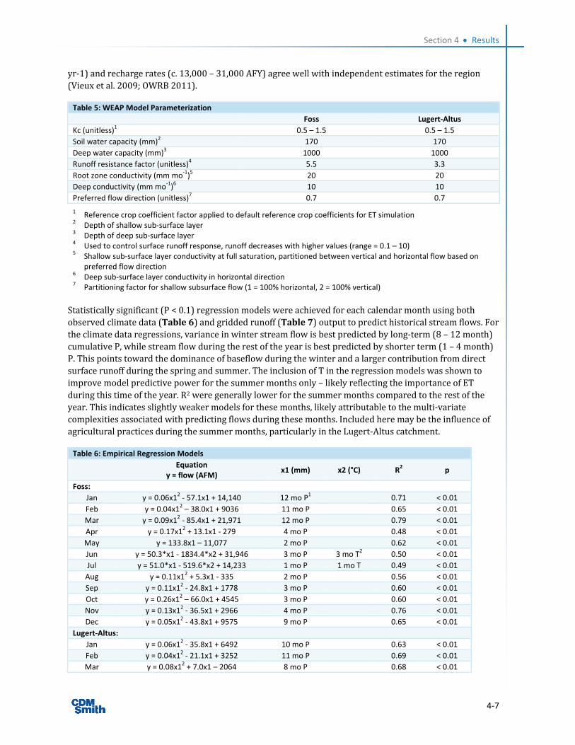
4.2 Hydrologic Model Parameterization The WEAP hydrologic model was calibrated using Washita River (Foss catchment) historical data and verified, with only minor parameter adjustments, using the Lugert‐Altus catchment model and historical N. Fork Red River data (Table 5). Annual water balances using the WEAP output indicate that ET losses account for c. 95 percent of the total precipitation falling on the two catchments. Modeled ET rates (c. 23 in

0

5

10

15

20

25

0 0.2 0.4 0.6 0.8 1

temperature ('C)

percentile

A2

stochastic ensemble 1 stochastic ensemble 2


stochastic ensemble 5 hybrid delta ensemble

full pooled data set

0

100

200

300

400

500

600

700

800

900

1000

0 0.2 0.4 0.6 0.8 1

precipitation (mm)

percentile

A2





‐10

‐5

0

5

10

15

20

25

30

35

40

0 0.2 0.4 0.6 0.8 1

temperature ('C)

percentile

A2





0

50

100

150

200

250

300

350

400

0 0.2 0.4 0.6 0.8 1

precipitation (mm)

percentile

A2





Section 4 Results

4‐7

yr‐1) and recharge rates (c. 13,000 – 31,000 AFY) agree well with independent estimates for the region (Vieux et al. 2009; OWRB 2011).

Table 5: WEAP Model Parameterization

Foss Lugert‐Altus

Kc (unitless)1 0.5 – 1.5 0.5 – 1.5

Soil water capacity (mm)2 170 170

Deep water capacity (mm)3 1000 1000

Runoff resistance factor (unitless)4 5.5 3.3

Root zone conductivity (mm mo‐1)5 20 20

Deep conductivity (mm mo‐1)6 10 10

Preferred flow direction (unitless)7 0.7 0.7

1 Reference crop coefficient factor applied to default reference crop coefficients for ET simulation 2 Depth of shallow sub‐surface layer 3 Depth of deep sub‐surface layer 4 Used to control surface runoff response, runoff decreases with higher values (range = 0.1 – 10) 5 Shallow sub‐surface layer conductivity at full saturation, partitioned between vertical and horizontal flow based on

preferred flow direction 6 Deep sub‐surface layer conductivity in horizontal direction 7 Partitioning factor for shallow subsurface flow (1 = 100% horizontal, 2 = 100% vertical)

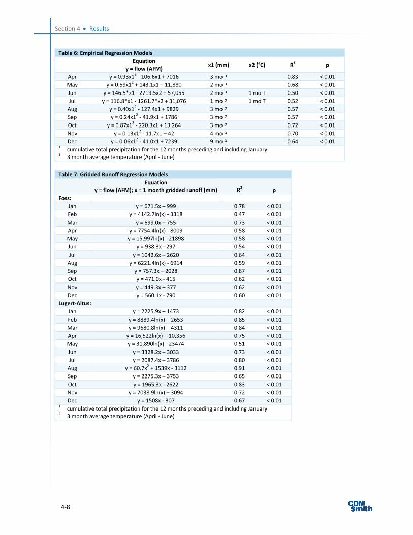
Statistically significant (P < 0.1) regression models were achieved for each calendar month using both observed climate data (Table 6) and gridded runoff (Table 7) output to predict historical stream flows. For the climate data regressions, variance in winter stream flow is best predicted by long‐term (8 – 12 month) cumulative P, while stream flow during the rest of the year is best predicted by shorter term (1 – 4 month) P. This points toward the dominance of baseflow during the winter and a larger contribution from direct surface runoff during the spring and summer. The inclusion of T in the regression models was shown to improve model predictive power for the summer months only – likely reflecting the importance of ET during this time of the year. R2 were generally lower for the summer months compared to the rest of the year. This indicates slightly weaker models for these months, likely attributable to the multi‐variate complexities associated with predicting flows during these months. Included here may be the influence of agricultural practices during the summer months, particularly in the Lugert‐Altus catchment.

Table 6: Empirical Regression Models

Equation

y = flow (AFM) x1 (mm) x2 (°C) R2 p

Foss:

Jan y = 0.06x12 ‐ 57.1x1 + 14,140 12 mo P1 0.71 < 0.01

Feb y = 0.04x12 – 38.0x1 + 9036 11 mo P 0.65 < 0.01

Mar y = 0.09x12 ‐ 85.4x1 + 21,971 12 mo P 0.79 < 0.01

Apr y = 0.17x12 + 13.1x1 ‐ 279 4 mo P 0.48 < 0.01

May y = 133.8x1 – 11,077 2 mo P 0.62 < 0.01

Jun y = 50.3*x1 ‐ 1834.4*x2 + 31,946 3 mo P 3 mo T2 0.50 < 0.01

Jul y = 51.0*x1 ‐ 519.6*x2 + 14,233 1 mo P 1 mo T 0.49 < 0.01

Aug y = 0.11x12 + 5.3x1 ‐ 335 2 mo P 0.56 < 0.01

Sep y = 0.11x12 ‐ 24.8x1 + 1778 3 mo P 0.60 < 0.01

Oct y = 0.26x12 – 66.0x1 + 4545 3 mo P 0.60 < 0.01

Nov y = 0.13x12 ‐ 36.5x1 + 2966 4 mo P 0.76 < 0.01

Dec y = 0.05x12 ‐ 43.8x1 + 9575 9 mo P 0.65 < 0.01

Lugert‐Altus:

Jan y = 0.06x12 ‐ 35.8x1 + 6492 10 mo P 0.63 < 0.01

Feb y = 0.04x12 ‐ 21.1x1 + 3252 11 mo P 0.69 < 0.01

Mar y = 0.08x12 + 7.0x1 – 2064 8 mo P 0.68 < 0.01

Section 4 Results

4‐8

Table 6: Empirical Regression Models

Equation

y = flow (AFM) x1 (mm) x2 (°C) R

2 p

Apr y = 0.93x12 ‐ 106.6x1 + 7016 3 mo P 0.83 < 0.01

May y = 0.59x12 + 143.1x1 – 11,880 2 mo P 0.68 < 0.01

Jun y = 146.5*x1 ‐ 2719.5x2 + 57,055 2 mo P 1 mo T 0.50 < 0.01

Jul y = 116.8*x1 ‐ 1261.7*x2 + 31,076 1 mo P 1 mo T 0.52 < 0.01

Aug y = 0.40x12 ‐ 127.4x1 + 9829 3 mo P 0.57 < 0.01

Sep y = 0.24x12 ‐ 41.9x1 + 1786 3 mo P 0.57 < 0.01

Oct y = 0.87x12 ‐ 220.3x1 + 13,264 3 mo P 0.72 < 0.01

Nov y = 0.13x12 ‐ 11.7x1 – 42 4 mo P 0.70 < 0.01

Dec y = 0.06x12 ‐ 41.0x1 + 7239 9 mo P 0.64 < 0.01 1 cumulative total precipitation for the 12 months preceding and including January 2 3 month average temperature (April ‐ June)

Table 7: Gridded Runoff Regression Models

Equation

y = flow (AFM); x = 1 month gridded runoff (mm) R2 p

Foss:

Jan y = 671.5x – 999 0.78 < 0.01

Feb y = 4142.7ln(x) ‐ 3318 0.47 < 0.01

Mar y = 699.0x – 755 0.73 < 0.01

Apr y = 7754.4ln(x) ‐ 8009 0.58 < 0.01

May y = 15,997ln(x) ‐ 21898 0.58 < 0.01

Jun y = 938.3x ‐ 297 0.54 < 0.01

Jul y = 1042.6x – 2620 0.64 < 0.01

Aug y = 6221.4ln(x) ‐ 6914 0.59 < 0.01

Sep y = 757.3x – 2028 0.87 < 0.01

Oct y = 471.0x ‐ 415 0.62 < 0.01

Nov y = 449.3x – 377 0.62 < 0.01

Dec y = 560.1x ‐ 790 0.60 < 0.01

Lugert‐Altus:

Jan y = 2225.9x – 1473 0.82 < 0.01

Feb y = 8889.4ln(x) – 2653 0.85 < 0.01

Mar y = 9680.8ln(x) – 4311 0.84 < 0.01

Apr y = 16,522ln(x) – 10,356 0.75 < 0.01

May y = 31,890ln(x) ‐ 23474 0.51 < 0.01

Jun y = 3328.2x – 3033 0.73 < 0.01

Jul y = 2087.4x – 3786 0.80 < 0.01

Aug y = 60.7x2 + 1539x ‐ 3112 0.91 < 0.01

Sep y = 2275.3x – 3753 0.65 < 0.01

Oct y = 1965.3x ‐ 2622 0.83 < 0.01

Nov y = 7038.9ln(x) – 3094 0.72 < 0.01

Dec y = 1508x ‐ 307 0.67 < 0.01 1 cumulative total precipitation for the 12 months preceding and including January 2 3 month average temperature (April ‐ June)

Section 4 Results

4‐9

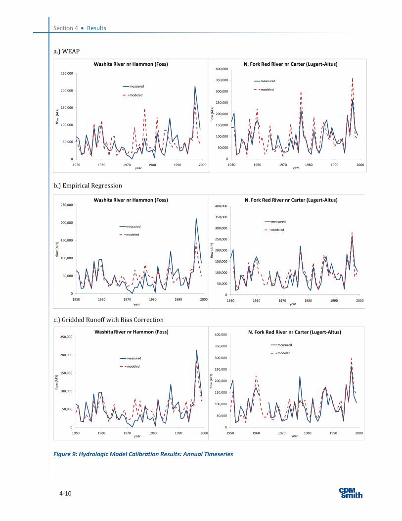
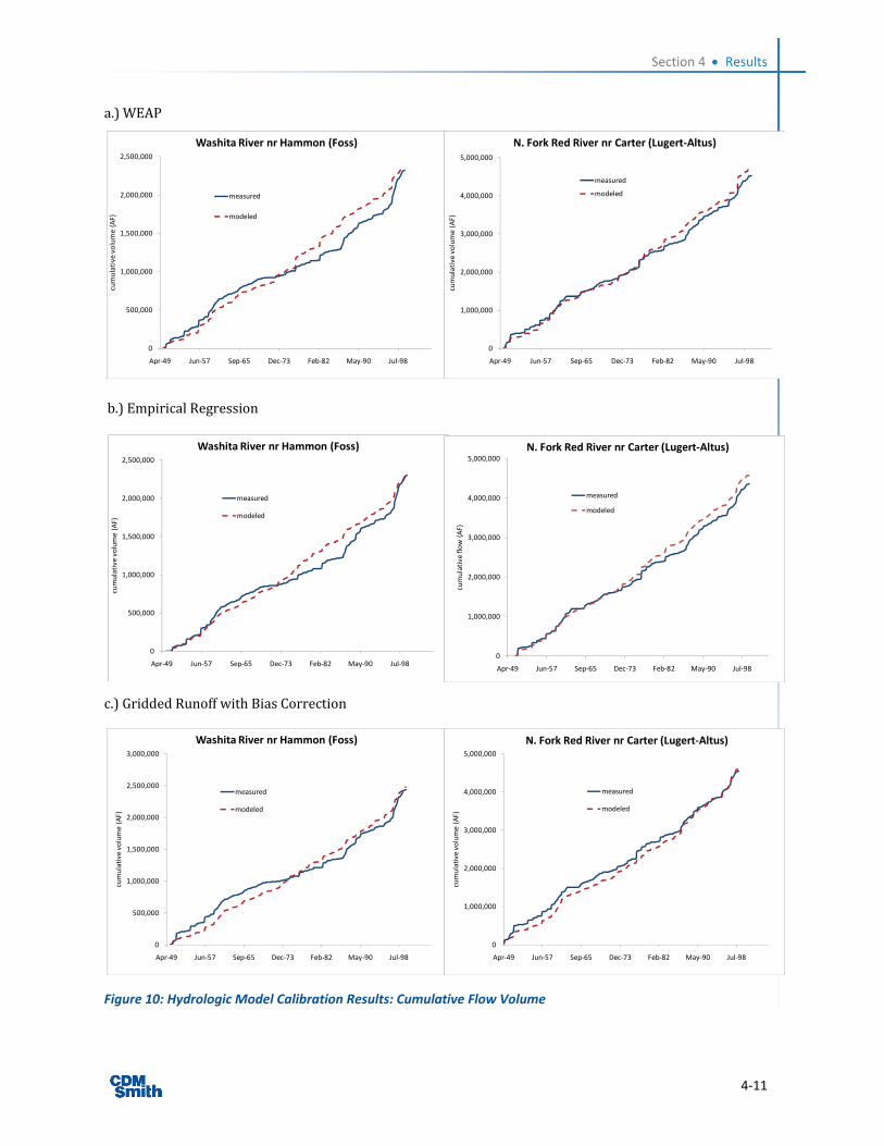
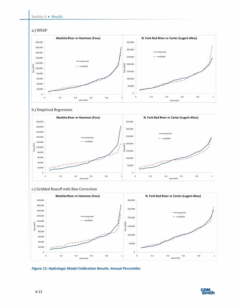
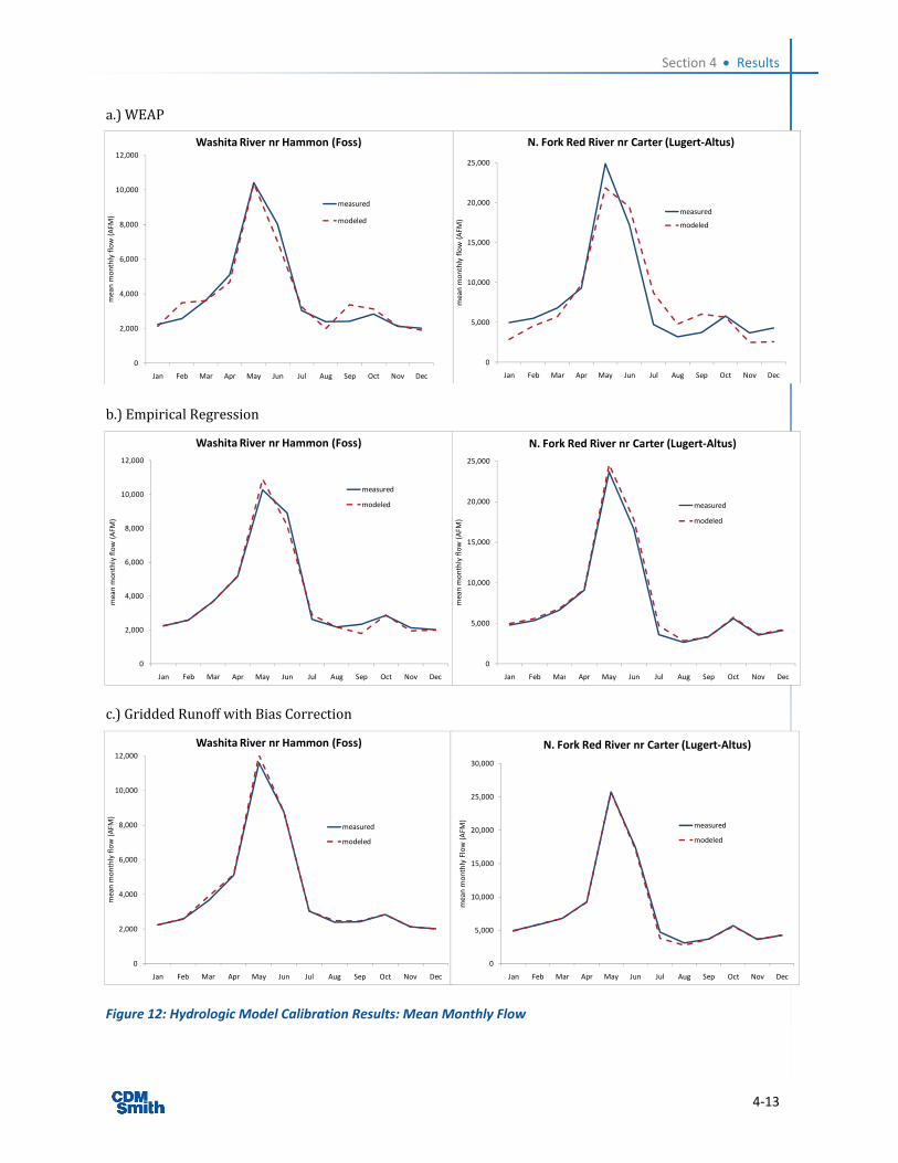
All three modeling approaches were able to adequately simulate historical stream flows in both catchments, based on multiple relevant hydrologic metrics (Figures 9 – 12). Based on visual inspection, the three modeling approaches appear to perform similarly in simulating annual flow variability (Figures 9 – 11). The regression models do a better job than WEAP at simulating mean monthly variations (Figure 12). However, this is not surprising since the models were developed by fitting equations, on a month‐by‐month basis, to the aggregate data set, based on an aggregate metric (RMSE). The WEAP model has a greater tendency to over‐predict upper percentile (high) annual flows compared to the other models (Figures 9 and 11). The Foss catchment empirical regression model does a poorer job of simulating the full range of annual flows observed in the calibration period, compared to the other models (Figure 11b). Goodness of fit parameters (Table 8) indicate that, overall, the simple regression models perform as well as, if not better than, the more sophisticated mechanistic WEAP model at simulating calibration period flows. It is noteworthy that none of the three modeling approaches are able to reproduce the measured low flow period of the early 1970s in the Foss Reservoir catchment (Figure 9). This period of data appears to be anomalous relative to climate conditions during this period and outside of the normal climate elasticities captured in the hydrologic models.

Section 4 Results

4‐10

a.) WEAP

b.) Empirical Regression

c.) Gridded Runoff with Bias Correction

Figure 9: Hydrologic Model Calibration Results: Annual Timeseries

0

50,000

100,000

150,000

200,000

250,000

1950 1960 1970 1980 1990 2000

flow (AFY)

year

Washita River nr Hammon (Foss)

measured

modeled

0

50,000

100,000

150,000

200,000

250,000

1950 1960 1970 1980 1990 2000

flow (AFY)

year


measured

modeled

0

50,000

100,000

150,000

200,000

250,000

1950 1960 1970 1980 1990 2000

flow (AFY)

year


measured

modeled

0

50,000

100,000

150,000

200,000

250,000

300,000

350,000

400,000

1950 1960 1970 1980 1990 2000

flow (AFY)

year

N. Fork Red River nr Carter (Lugert‐Altus)

measured

modeled

0

50,000

100,000

150,000

200,000

250,000

300,000

350,000

400,000

1950 1960 1970 1980 1990 2000

flow (AFY)

year


measured

modeled

0

50,000

100,000

150,000

200,000

250,000

300,000

350,000

400,000

1950 1960 1970 1980 1990 2000

flow (AFY)

year


measured

modeled

Section 4 Results

4‐11

a.) WEAP



Figure 10: Hydrologic Model Calibration Results: Cumulative Flow Volume

0

500,000

1,000,000

1,500,000

2,000,000

2,500,000

Apr‐49 Jun‐57 Sep‐65 Dec‐73 Feb‐82 May‐90 Jul‐98

cumulative volume (AF)


measured

modeled

0

500,000

1,000,000

1,500,000

2,000,000

2,500,000




measured

modeled

0

500,000

1,000,000

1,500,000

2,000,000

2,500,000

3,000,000




measured

modeled

0

1,000,000

2,000,000

3,000,000

4,000,000

5,000,000




measured

modeled

0

1,000,000

2,000,000

3,000,000

4,000,000

5,000,000


cumulative flow (AF)


measured

modeled

0

1,000,000

2,000,000

3,000,000

4,000,000

5,000,000




measured

modeled

Section 4 Results

4‐12

a.) WEAP



Figure 11: Hydrologic Model Calibration Results: Annual Percentiles

0

20,000

40,000

60,000

80,000

100,000

120,000

140,000

160,000

180,000

200,000

0 0.2 0.4 0.6 0.8 1

flow (AFY)

percentile


measured

modeled

0

20,000

40,000

60,000

80,000

100,000

120,000

140,000

160,000

180,000

200,000

0 0.2 0.4 0.6 0.8 1

flow (AFY)

percentile


measured

modeled

0

20,000

40,000

60,000

80,000

100,000

120,000

140,000

160,000

180,000

200,000

0 0.2 0.4 0.6 0.8 1

flow (AFY)

percentile


measured

modeled

0

50,000

100,000

150,000

200,000

250,000

300,000

350,000

0 0.2 0.4 0.6 0.8 1

flow (AFM

)

percentile


measured

modeled

0

50,000

100,000

150,000

200,000

250,000

300,000

350,000

0 0.2 0.4 0.6 0.8 1

flow (AFY)

percentile


measured

modeled

0

50,000

100,000

150,000

200,000

250,000

300,000

0 0.2 0.4 0.6 0.8 1

flow (AFM

)

percentile


measured

modeled

Section 4 Results

4‐13

a.) WEAP



Figure 12: Hydrologic Model Calibration Results: Mean Monthly Flow

0

2,000

4,000

6,000

8,000

10,000

12,000


mean m

onthly flow (AFM

)


measured

modeled

0

2,000

4,000

6,000

8,000

10,000

12,000


mean m

onthly flow (AFM

)


measured

modeled

0

2,000

4,000

6,000

8,000

10,000

12,000


mean m

onthly flow (AFM

)


measured

modeled

0

5,000

10,000

15,000

20,000

25,000


mean m

onthly flow (AFM

)


measured

modeled

0

5,000

10,000

15,000

20,000

25,000


mean m

onthly flow (AFM

)


measured

modeled

0

5,000

10,000

15,000

20,000

25,000

30,000


mean m

onthly Flow (AFM

)


measured

modeled

Section 4 Results

4‐14

Table 8: Model Calibration Statistics

RMSE (AFM) R2

Foss WEAP 6207 0.46

Foss Empirical Regression 4071 0.64

Foss Gridded Runoff w/ Bias Correction 4082 0.68

Lugert‐Altus WEAP 10,169 0.70

Lugert‐Altus Empirical Regression 7564 0.73

Lugert‐Altus Gridded Runoff w/ Bias Correction 8007 0.70

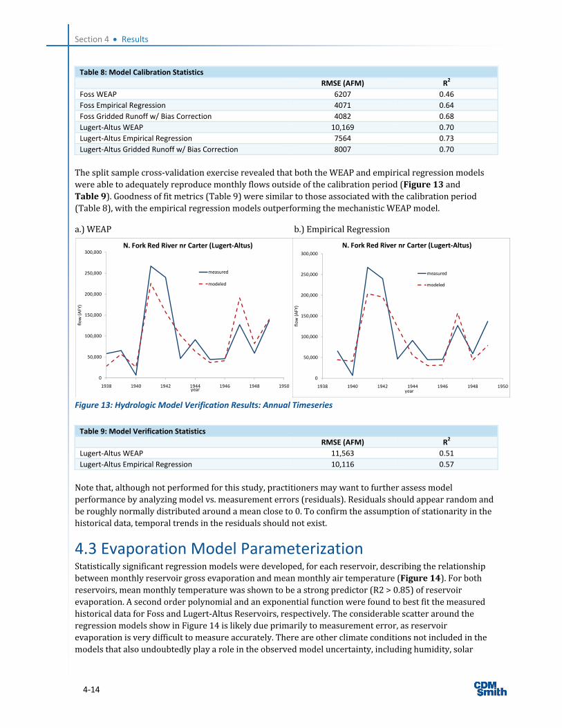
The split sample cross‐validation exercise revealed that both the WEAP and empirical regression models were able to adequately reproduce monthly flows outside of the calibration period (Figure 13 and Table 9). Goodness of fit metrics (Table 9) were similar to those associated with the calibration period (Table 8), with the empirical regression models outperforming the mechanistic WEAP model.

a.) WEAP b.) Empirical Regression

Figure 13: Hydrologic Model Verification Results: Annual Timeseries

Table 9: Model Verification Statistics

RMSE (AFM) R2

Lugert‐Altus WEAP 11,563 0.51

Lugert‐Altus Empirical Regression 10,116 0.57

Note that, although not performed for this study, practitioners may want to further assess model performance by analyzing model vs. measurement errors (residuals). Residuals should appear random and be roughly normally distributed around a mean close to 0. To confirm the assumption of stationarity in the historical data, temporal trends in the residuals should not exist.

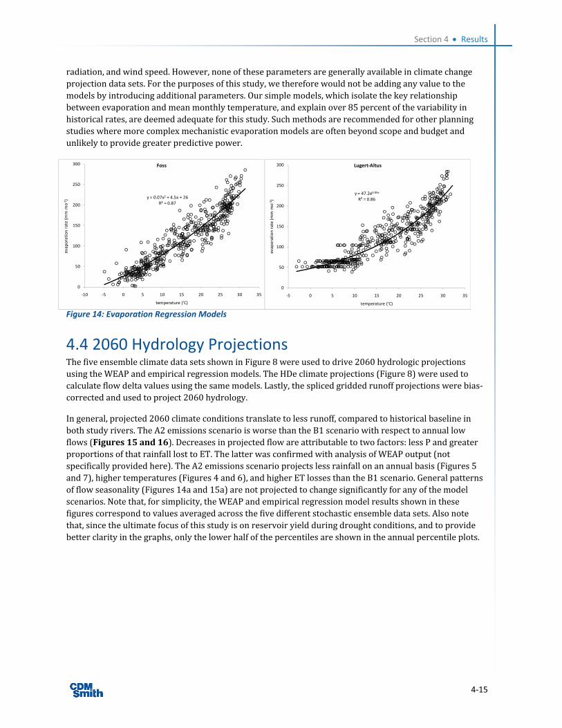
4.3 Evaporation Model Parameterization Statistically significant regression models were developed, for each reservoir, describing the relationship between monthly reservoir gross evaporation and mean monthly air temperature (Figure 14). For both reservoirs, mean monthly temperature was shown to be a strong predictor (R2 > 0.85) of reservoir evaporation. A second order polynomial and an exponential function were found to best fit the measured historical data for Foss and Lugert‐Altus Reservoirs, respectively. The considerable scatter around the regression models show in Figure 14 is likely due primarily to measurement error, as reservoir evaporation is very difficult to measure accurately. There are other climate conditions not included in the models that also undoubtedly play a role in the observed model uncertainty, including humidity, solar

0

50,000

100,000

150,000

200,000

250,000

300,000

1938 1940 1942 1944 1946 1948 1950

flow (AFY)

year


measured

modeled

0

50,000

100,000

150,000

200,000

250,000

300,000

1938 1940 1942 1944 1946 1948 1950

flow (AFY)

year


measured

modeled

Section 4 Results

4‐15

radiation, and wind speed. However, none of these parameters are generally available in climate change projection data sets. For the purposes of this study, we therefore would not be adding any value to the models by introducing additional parameters. Our simple models, which isolate the key relationship between evaporation and mean monthly temperature, and explain over 85 percent of the variability in historical rates, are deemed adequate for this study. Such methods are recommended for other planning studies where more complex mechanistic evaporation models are often beyond scope and budget and unlikely to provide greater predictive power.

Figure 14: Evaporation Regression Models

4.4 2060 Hydrology Projections The five ensemble climate data sets shown in Figure 8 were used to drive 2060 hydrologic projections using the WEAP and empirical regression models. The HDe climate projections (Figure 8) were used to calculate flow delta values using the same models. Lastly, the spliced gridded runoff projections were bias‐corrected and used to project 2060 hydrology.

In general, projected 2060 climate conditions translate to less runoff, compared to historical baseline in both study rivers. The A2 emissions scenario is worse than the B1 scenario with respect to annual low flows (Figures 15 and 16). Decreases in projected flow are attributable to two factors: less P and greater proportions of that rainfall lost to ET. The latter was confirmed with analysis of WEAP output (not specifically provided here). The A2 emissions scenario projects less rainfall on an annual basis (Figures 5 and 7), higher temperatures (Figures 4 and 6), and higher ET losses than the B1 scenario. General patterns of flow seasonality (Figures 14a and 15a) are not projected to change significantly for any of the model scenarios. Note that, for simplicity, the WEAP and empirical regression model results shown in these figures correspond to values averaged across the five different stochastic ensemble data sets. Also note that, since the ultimate focus of this study is on reservoir yield during drought conditions, and to provide better clarity in the graphs, only the lower half of the percentiles are shown in the annual percentile plots.

y = 0.07x2 + 4.5x + 26R² = 0.87

0

50

100

150

200

250

300

‐10 ‐5 0 5 10 15 20 25 30 35

evaporation rate (m

m m

o‐1)

temperature ('C)

Foss

y = 47.2e0.05x

R² = 0.86

0

50

100

150

200

250

300

‐5 0 5 10 15 20 25 30 35

evaporation rate (m

m m

o‐1)

temperature ('C)

Lugert‐Altus

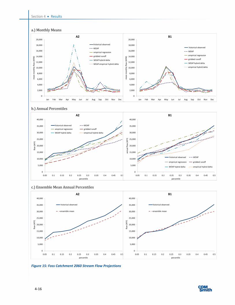
Section 4 Results

4‐16

a.) Monthly Means

b.) Annual Percentiles

c.) Ensemble Mean Annual Percentiles

Figure 15: Foss Catchment 2060 Stream Flow Projections

0

2,000

4,000

6,000

8,000

10,000

12,000

14,000

16,000

18,000

20,000


mean m

onthly flow (AFM

)

A2

historical observed

WEAP

empirical regression

gridded runoff

WEAP hybrid delta

WEAP empirical hybrid delta

0

2,000

4,000

6,000

8,000

10,000

12,000

14,000

16,000

18,000

20,000


mean m

onthly flow (AFM

)

B1

historical observed

WEAP


gridded runoff

WEAP hybrid delta

empirical hybrid delta

0

5,000

10,000

15,000

20,000

25,000

30,000

35,000

40,000

0.05 0.1 0.15 0.2 0.25 0.3 0.35 0.4 0.45 0.5

flow (AFY)

percentile

A2

historical observed WEAP

empirical regression gridded runoff

WEAP hybrid delta empirical hybrid delta

0

5,000

10,000

15,000

20,000

25,000

30,000

35,000

40,000

0.05 0.1 0.15 0.2 0.25 0.3 0.35 0.4 0.45 0.5

annual flow (AFY)

percentile

B1




0

5,000

10,000

15,000

20,000

25,000

30,000

35,000

40,000

0.05 0.1 0.15 0.2 0.25 0.3 0.35 0.4 0.45 0.5

flow (AFY)

percentile

A2

historical observed

ensemble mean

0

5,000

10,000

15,000

20,000

25,000

30,000

35,000

40,000

0.05 0.1 0.15 0.2 0.25 0.3 0.35 0.4 0.45 0.5

flow (AFY)

percentile

B1

historical observed

ensemble mean

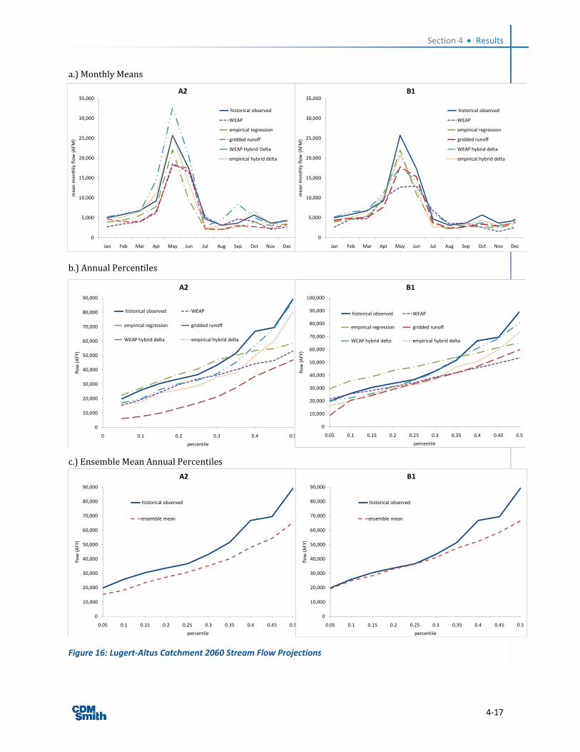
Section 4 Results

4‐17

a.) Monthly Means

b.) Annual Percentiles

c.) Ensemble Mean Annual Percentiles

Figure 16: Lugert‐Altus Catchment 2060 Stream Flow Projections

0

5,000

10,000

15,000

20,000

25,000

30,000

35,000


mean m

onthly flow (AFM

)

A2

historical observed

WEAP


gridded runoff

WEAP Hybrid Delta


0

5,000

10,000

15,000

20,000

25,000

30,000

35,000


mean m

onthly flow (AFM

)

B1

historical observed

WEAP


gridded runoff

WEAP hybrid delta


0

10,000

20,000

30,000

40,000

50,000

60,000

70,000

80,000

90,000

0 0.1 0.2 0.3 0.4 0.5

flow (AFY)

percentile

A2




0

10,000

20,000

30,000

40,000

50,000

60,000

70,000

80,000

90,000

100,000

0.05 0.1 0.15 0.2 0.25 0.3 0.35 0.4 0.45 0.5

flow (AFY)

percentile

B1




0

10,000

20,000

30,000

40,000

50,000

60,000

70,000

80,000

90,000

0.05 0.1 0.15 0.2 0.25 0.3 0.35 0.4 0.45 0.5

flow (AFY)

percentile

A2

historical observed

ensemble mean

0

10,000

20,000

30,000

40,000

50,000

60,000

70,000

80,000

90,000

0.05 0.1 0.15 0.2 0.25 0.3 0.35 0.4 0.45 0.5

flow (AFY)

percentile

B1

historical observed

ensemble mean

Section 4 Results

4‐18

In addition to the sensitivity to assumed greenhouse gas emissions, we see a reasonably high sensitivity to the selected hydrologic modeling approach, with mean annual flows ranging from 32,000 to 61,000 AFY for Foss and from 68,000 to 114,000 AFY for Lugert‐Altus. The WEAP model used within the HDe approach actually predicts a significant increase in spring (Apr – Jun) high flows on a mean monthly basis, compared to baseline, for both catchments (Figures 14a and 15a). This is largely the result of the simulation of a few unusually high flow months by this method that skew the mean metric. These high flow predictions occur within the HDe method because of two factors. Firstly, the ratio method used to adjust historical precipitation records can result in monthly precipitation values higher than any either observed or simulated by the climate models. Secondly, since these precipitation values are outside the range of calibration data, the WEAP model may over‐estimate the stream flow response to high precipitation events. On the other hand, the WEAP model by itself projects a decrease (c. 10 – 60 percent) in mean monthly flows particularly during the peak flow season. These two results together indicate a threshold in the calibrated WEAP model, likely linked to the depth of the calibrated shallow sub‐surface zone. Spring precipitation above this threshold, as in the HDe data set, results in saturation conditions and large volumes of immediate runoff. Spring precipitation below this threshold gets largely stored and the runoff response is dampened.

All models except the B1 empirical regression model project annual low flows for the 2060 climate condition that are less than or equal to baseline (Figures 14b and 15b). Projected decreases in annual flows range up to approximately 50 percent (e.g., gridded runoff A2 model). Ensemble means, averaged across all hydrologic projections, indicate a projected decrease in annual low flows of approximately 10 – 25 percent for the A2 scenario and both catchments (Figure 14c and 15c). For the B1 scenario, projected low flows are approximately equal to baseline values up to approximately the 30th percentile, from which they decrease relative to baseline to approximately 20 – 30 percent lower for the median annual flows.

Use of the newly available gridded runoff data set, with bias correction, results in annual low flow projections that are low relative to the consensus of other hydrologic modeling approaches included in this study. However, this appears to be more a function of the ensemble precipitation data underlying the flow projections (Figure 8a) than of the hydrologic model itself or the bias correction method. No other consistent trends were identified in the comparison of hydrologic model projections.

4.5 2060 Evaporation Projections Application of the empirical regression evaporation models with the various 2060 climate projections resulted in an increase in mean annual net evaporation of approximately 42 percent and 26 percent, for the A2 and B1 emissions scenarios respectively, compared to historical observed rates (Table 10). These values were averaged across all ensembled climate data sets and were approximately the same for the two basins. Percentile plots (Figure 17) reveal consistency in the magnitudes of increases predicted by the modeling across the range of cool to warm years.

Table 10: Mean Annual Net Evaporation Projections

Historical Mean 2060 A2 Mean 2060 B1

Net Evaporation (mm yr‐1) 790 1120 990

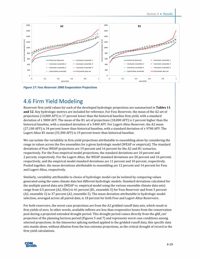
Section 4 Results

4‐19

Figure 17: Foss Reservoir 2060 Evaporation Projections

4.6 Firm Yield Modeling Reservoir firm yield values for each of the developed hydrologic projections are summarized in Tables 11 and 12. Key hydrologic metrics are included for reference. For Foss Reservoir, the mean of the A2 set of projections (14,800 AFY) is 17 percent lower than the historical baseline firm yield, with a standard deviation of ± 5800 AFY. The mean of the B1 set of projections (18,000 AFY) is 2 percent higher than the historical baseline, with a standard deviation of ± 5400 AFY. For Lugert‐Altus Reservoir, the A2 mean (27,100 AFY) is 34 percent lower than historical baseline, with a standard deviation of ± 9700 AFY. The Lugert‐Altus B1 mean (33,300 AFY) is 19 percent lower than historical baseline.

We can isolate the variability in firm yield projections attributable to ensembling alone by considering the range in values across the five ensembles for a given hydrologic model (WEAP or empirical). The standard deviations of Foss WEAP projections are 19 percent and 16 percent for the A2 and B1 scenarios, respectively. For the Foss empirical model projections, the standard deviations are 10 percent and 2 percent, respectively. For the Lugert‐Altus, the WEAP standard deviations are 20 percent and 16 percent, respectively, and the empirical model standard deviations are 11 percent and 10 percent, respectively. Pooled together, the mean deviations attributable to ensembling are 12 percent and 14 percent for Foss and Lugert‐Altus, respectively.

Similarly, variability attributable to choice of hydrologic model can be isolated by comparing values generated using the same climate data but different hydrologic models. Standard deviations calculated for the multiple paired data sets (WEAP vs. empirical model using the various ensemble climate data sets) range from 0.5 percent (A2, HDe) to 41 percent (B1, ensemble 5) for Foss Reservoir and from 5 percent (A2, ensemble 2) to 37 percent (A2, ensemble 5). The mean deviation attributable to hydrologic model selection, averaged across all paired data, is 18 percent for both Foss and Lugert‐Altus Reservoirs.

For both reservoirs, the worst‐case projections are from the A2 gridded runoff data sets, which result in firm yields of zero. In other words, available inflows are less than evaporative losses from the conservation pool during a projected extended drought period. This drought period comes directly from the gfdl_cm2 projection of the planning horizon period (Figures 5 and 7) and represents worst case conditions among selected projections. In the timeseries splicing method applied to the gridded runoff data, this specific data sets stands alone, without dilution from the less extreme projections, as the critical drought of record in the firm yield calculations.

0

200

400

600

800

1000

1200

1400

1600

1800

0 0.2 0.4 0.6 0.8 1

annual net evaporation (mm)

percentile

A2

historical observed stochastic ensemble 1



hybrid delta ensemble full pooled data set

0

200

400

600

800

1000

1200

1400

1600

1800

0 0.2 0.4 0.6 0.8 1

annual net evaporation (mm)

percentile

B1

historical observed stochastic ensemble 1



hybrid delta ensemble full pooled data set

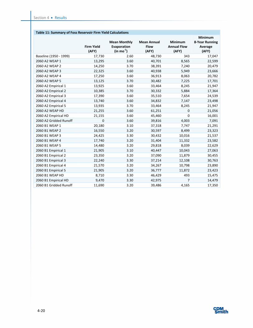
Section 4 Results

4‐20

Table 11: Summary of Foss Reservoir Firm Yield Calculations

Firm Yield (AFY)

Mean Monthly Evaporation (in mo‐1)

Mean Annual Flow (AFY)

Minimum Annual Flow

(AFY)

Minimum 8‐Year Running

Average (AFY)

Baseline (1950 ‐ 1999) 17,730 2.60 48,730 343 17,047

2060 A2 WEAP 1 13,295 3.60 40,701 8,565 22,599

2060 A2 WEAP 2 14,250 3.70 38,391 7,240 20,479

2060 A2 WEAP 3 22,325 3.60 40,938 5,949 23,666

2060 A2 WEAP 4 17,250 3.60 36,913 8,063 20,782

2060 A2 WEAP 5 13,125 3.70 30,482 7,225 17,701

2060 A2 Empirical 1 13,925 3.60 33,464 8,245 21,947

2060 A2 Empirical 2 10,385 3.70 30,332 5,884 17,364

2060 A2 Empirical 3 17,390 3.60 35,510 7,654 24,539

2060 A2 Empirical 4 13,740 3.60 34,832 7,147 23,498

2060 A2 Empirical 5 13,935 3.70 33,464 8,245 21,947

2060 A2 WEAP HD 21,255 3.60 61,251 0 21,056

2060 A2 Empirical HD 21,155 3.60 45,460 0 16,001

2060 A2 Gridded Runoff 0 3.60 39,816 4,003 7,091

2060 B1 WEAP 1 20,180 3.10 37,318 7,747 21,291

2060 B1 WEAP 2 16,550 3.20 30,597 8,499 23,323

2060 B1 WEAP 3 24,425 3.30 30,432 10,016 21,537

2060 B1 WEAP 4 17,740 3.20 31,404 11,332 23,582

2060 B1 WEAP 5 14,480 3.20 29,818 8,039 22,629

2060 B1 Empirical 1 21,905 3.10 40,447 10,043 27,063

2060 B1 Empirical 2 23,350 3.20 37,090 11,879 30,455

2060 B1 Empirical 3 22,240 3.30 37,214 12,108 30,763

2060 B1 Empirical 4 21,570 3.20 34,267 10,798 23,890

2060 B1 Empirical 5 21,905 3.20 36,777 11,872 23,423

2060 B1 WEAP HD 8,710 3.30 46,429 493 15,475

2060 B1 Empirical HD 9,470 3.30 42,975 7 14,479

2060 B1 Gridded Runoff 11,690 3.20 39,486 4,165 17,350

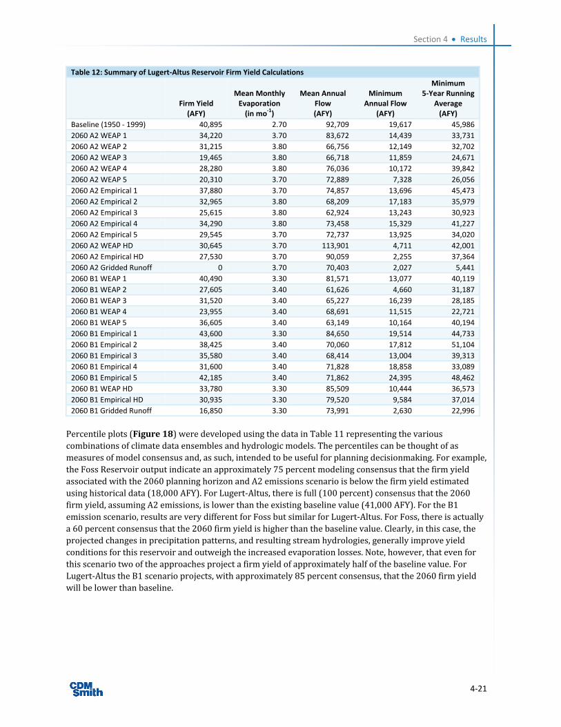
Section 4 Results

4‐21

Table 12: Summary of Lugert‐Altus Reservoir Firm Yield Calculations

Firm Yield (AFY)

Mean Monthly Evaporation (in mo‐1)

Mean Annual Flow (AFY)

Minimum Annual Flow

(AFY)

Minimum 5‐Year Running

Average (AFY)

Baseline (1950 ‐ 1999) 40,895 2.70 92,709 19,617 45,986

2060 A2 WEAP 1 34,220 3.70 83,672 14,439 33,731

2060 A2 WEAP 2 31,215 3.80 66,756 12,149 32,702

2060 A2 WEAP 3 19,465 3.80 66,718 11,859 24,671

2060 A2 WEAP 4 28,280 3.80 76,036 10,172 39,842

2060 A2 WEAP 5 20,310 3.70 72,889 7,328 26,056

2060 A2 Empirical 1 37,880 3.70 74,857 13,696 45,473

2060 A2 Empirical 2 32,965 3.80 68,209 17,183 35,979

2060 A2 Empirical 3 25,615 3.80 62,924 13,243 30,923

2060 A2 Empirical 4 34,290 3.80 73,458 15,329 41,227

2060 A2 Empirical 5 29,545 3.70 72,737 13,925 34,020

2060 A2 WEAP HD 30,645 3.70 113,901 4,711 42,001

2060 A2 Empirical HD 27,530 3.70 90,059 2,255 37,364

2060 A2 Gridded Runoff 0 3.70 70,403 2,027 5,441

2060 B1 WEAP 1 40,490 3.30 81,571 13,077 40,119

2060 B1 WEAP 2 27,605 3.40 61,626 4,660 31,187

2060 B1 WEAP 3 31,520 3.40 65,227 16,239 28,185

2060 B1 WEAP 4 23,955 3.40 68,691 11,515 22,721

2060 B1 WEAP 5 36,605 3.40 63,149 10,164 40,194

2060 B1 Empirical 1 43,600 3.30 84,650 19,514 44,733

2060 B1 Empirical 2 38,425 3.40 70,060 17,812 51,104

2060 B1 Empirical 3 35,580 3.40 68,414 13,004 39,313

2060 B1 Empirical 4 31,600 3.40 71,828 18,858 33,089

2060 B1 Empirical 5 42,185 3.40 71,862 24,395 48,462

2060 B1 WEAP HD 33,780 3.30 85,509 10,444 36,573

2060 B1 Empirical HD 30,935 3.30 79,520 9,584 37,014

2060 B1 Gridded Runoff 16,850 3.30 73,991 2,630 22,996

Percentile plots (Figure 18) were developed using the data in Table 11 representing the various combinations of climate data ensembles and hydrologic models. The percentiles can be thought of as measures of model consensus and, as such, intended to be useful for planning decisionmaking. For example, the Foss Reservoir output indicate an approximately 75 percent modeling consensus that the firm yield associated with the 2060 planning horizon and A2 emissions scenario is below the firm yield estimated using historical data (18,000 AFY). For Lugert‐Altus, there is full (100 percent) consensus that the 2060 firm yield, assuming A2 emissions, is lower than the existing baseline value (41,000 AFY). For the B1 emission scenario, results are very different for Foss but similar for Lugert‐Altus. For Foss, there is actually a 60 percent consensus that the 2060 firm yield is higher than the baseline value. Clearly, in this case, the projected changes in precipitation patterns, and resulting stream hydrologies, generally improve yield conditions for this reservoir and outweigh the increased evaporation losses. Note, however, that even for this scenario two of the approaches project a firm yield of approximately half of the baseline value. For Lugert‐Altus the B1 scenario projects, with approximately 85 percent consensus, that the 2060 firm yield will be lower than baseline.

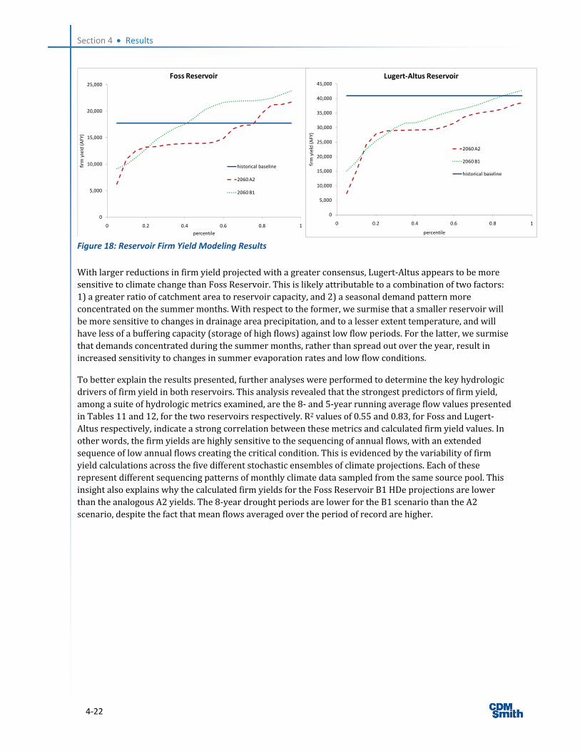
Section 4 Results

4‐22

Figure 18: Reservoir Firm Yield Modeling Results

With larger reductions in firm yield projected with a greater consensus, Lugert‐Altus appears to be more sensitive to climate change than Foss Reservoir. This is likely attributable to a combination of two factors: 1) a greater ratio of catchment area to reservoir capacity, and 2) a seasonal demand pattern more concentrated on the summer months. With respect to the former, we surmise that a smaller reservoir will be more sensitive to changes in drainage area precipitation, and to a lesser extent temperature, and will have less of a buffering capacity (storage of high flows) against low flow periods. For the latter, we surmise that demands concentrated during the summer months, rather than spread out over the year, result in increased sensitivity to changes in summer evaporation rates and low flow conditions.

To better explain the results presented, further analyses were performed to determine the key hydrologic drivers of firm yield in both reservoirs. This analysis revealed that the strongest predictors of firm yield, among a suite of hydrologic metrics examined, are the 8‐ and 5‐year running average flow values presented in Tables 11 and 12, for the two reservoirs respectively. R2 values of 0.55 and 0.83, for Foss and Lugert‐Altus respectively, indicate a strong correlation between these metrics and calculated firm yield values. In other words, the firm yields are highly sensitive to the sequencing of annual flows, with an extended sequence of low annual flows creating the critical condition. This is evidenced by the variability of firm yield calculations across the five different stochastic ensembles of climate projections. Each of these represent different sequencing patterns of monthly climate data sampled from the same source pool. This insight also explains why the calculated firm yields for the Foss Reservoir B1 HDe projections are lower than the analogous A2 yields. The 8‐year drought periods are lower for the B1 scenario than the A2 scenario, despite the fact that mean flows averaged over the period of record are higher.

0

5,000

10,000

15,000

20,000

25,000

0 0.2 0.4 0.6 0.8 1

firm

yield (AFY)

percentile

Foss Reservoir

historical baseline

2060 A2

2060 B1

0

5,000

10,000

15,000

20,000

25,000

30,000

35,000

40,000

45,000

0 0.2 0.4 0.6 0.8 1

firm

yield (AFY)

percentile

Lugert‐Altus Reservoir

2060 A2

2060 B1

historical baseline

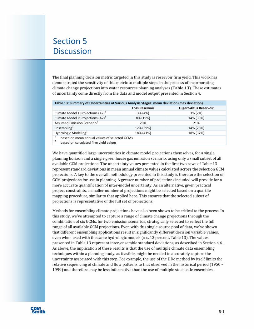
5‐1

Section 5 Discussion

The final planning decision metric targeted in this study is reservoir firm yield. This work has demonstrated the sensitivity of this metric to multiple steps in the process of incorporating climate change projections into water resources planning analyses (Table 13). These estimates of uncertainty come directly from the data and model output presented in Section 4.

Table 13: Summary of Uncertainties at Various Analysis Stages: mean deviation (max deviation)

Foss Reservoir Lugert‐Altus Reservoir

Climate Model T Projections (A2)1 3% (4%) 3% (7%)

Climate Model P Projections (A2)1 8% (19%) 14% (33%)

Assumed Emission Scenario2 20% 21%

Ensembling2 12% (39%) 14% (28%)

Hydrologic Modeling2 18% (41%) 18% (37%) 1 based on mean annual values of selected GCMs 2 based on calculated firm yield values

We have quantified large uncertainties in climate model projections themselves, for a single planning horizon and a single greenhouse gas emission scenario, using only a small subset of all available GCM projections. The uncertainty values presented in the first two rows of Table 13 represent standard deviations in mean annual climate values calculated across the selection GCM projections. A key to the overall methodology presented in this study is therefore the selection of GCM projections for use in planning. A greater number of projections included will provide for a more accurate quantification of inter‐model uncertainty. As an alternative, given practical project constraints, a smaller number of projections might be selected based on a quartile mapping procedure, similar to that applied here. This ensures that the selected subset of projections is representative of the full set of projections.

Methods for ensembling climate projections have also been shown to be critical to the process. In this study, we've attempted to capture a range of climate change projections through the combination of six GCMs, for two emission scenarios, strategically selected to reflect the full range of all available GCM projections. Even with this single source pool of data, we've shown that different ensembling applications result in significantly different decision variable values, even when used with the same hydrologic models (± c. 13 percent, Table 13). The values presented in Table 13 represent inter‐ensemble standard deviations, as described in Section 4.6. As above, the implication of these results is that the use of multiple climate data ensembling techniques within a planning study, as feasible, might be needed to accurately capture the uncertainty associated with this step. For example, the use of the HDe method by itself limits the relative sequencing of climate and flow patterns to that observed in the historical period (1950 – 1999) and therefore may be less informative than the use of multiple stochastic ensembles.


5‐2

Uncertainty associated with choice of hydrologic models appears to be as great as, or greater than, that associated with other steps in the process (± 18 percent, Table 13). As described in Section 4.6, the values presented in this table represent the means of inter‐model variations averaged across all firm yield projection pairs (WEAP vs. empirical model) corresponding to the same input climate ensemble. The HDe and gridded runoff projections were not included in this calculation since they are forced by different climate data, and thus the impacts of model structure alone could not be isolated. Since the focus is on low flows here, the results presented in Table 13 do not appear to contradict the results of recent studies by Gosling et al. (2011) and Maurer et al. (2010). Uncertainty is reduced through accurate model calibration and parameterization using historical data and based on multiple output metrics – particularly those to which final decision variables are most sensitive. Given the results presented here, the use of hydrologic models that have not been calibrated or parameterized at a catchment scale is not recommended for these types of studies. However, even with calibration, we see large uncertainties in predictions of the future where much of the climate conditions fall outside the range observed in the calibration period. Despite this uncertainty, there is general consensus among the models that stream flows will decrease in the future, given either emission scenario, on a mean monthly and annual total basis. Median annual flows, averaged across all scenarios, are projected to be approximately 15 and 25 percent lower than baseline for the two reservoirs, respectively. This agrees well with previous OWRB estimates (AMEC 2010). However, we also observe a seemingly significant difference between the two emission scenarios (A2 and B1) with respect to stream flow projections. The projected ensemble means of low percentile annual flows are only slightly lower than baseline for the B1 scenario, for both catchments, but are upwards of 25 percent lower for the A2 scenario. This result points towards the importance of greenhouse gas mitigation now and in the future.

Hydrologic modeling of the historical period indicates that simple regression models can perform as well as, if not better than, more sophisticated mechanistic approaches with respect to simulating flow – climate dependencies. This is supported by results of a split sample cross‐validation exercise. There are obvious cost‐saving implications here. Establishing simple regression relationships between stream flow and climate variables, or stream flow and macro‐scale gridded runoff output, requires less expertise, and likely less time, than constructing and calibrating a catchment‐level mechanistic model (e.g., WEAP). We propose that the marginal time and cost associated with more complex hydrologic modeling might be better spent on capturing uncertainties in the climate projections, as described above. Clearly this recommendation assumes adequate availability of site‐specific gaged flow data. If such data do not exist, generalized mechanistic models may be more appropriate. Further, there are likely many applications where regression models will not be sufficient. For example, studies that look to simulate basin changes beyond just climate would likely require explicit representation of specific catchment processes (i.e., mechanistic models). The lumped regression approach would also fall short if spatial resolution in flow simulations is needed. More complex basins might also require more complex models. These could include basins with snowpack driven hydrologies, more varied landscape and topography, and/or greater in‐basin water use and storage. Lastly, regression models may, arguably, be subject to greater uncertainty, compared to mechanistic models, when extended beyond the range of the calibration data set. Ultimately, the validity of simple vs. complex hydrologic models should be assessed on a case by case basis.

Newly available gridded runoff projections are shown to be poor predictors of stream flow by themselves, for the study basins, and require bias correction for application at a catchment scale. Catchment runoff is over‐predicted by the VIC model. A small portion of this error is likely attributable to upstream municipal diversions and consumption. However, based on water balances derived from the WEAP modeling, it is likely that a majority of this error stems from underestimates of ET losses and groundwater recharge. Recent Reclamation studies (Reclamation 2011) have shown that these projections are more accurate for larger spatial and temporal scales. This is due to a smoothing effect as water moves through larger basins and over longer time intervals, which tends to averages out small‐scale errors.


5‐3

One option for bias correction of the gridded runoff data set has been demonstrated in this study. This technique involves monthly regression analysis using historical stream flow data and gridded runoff output, corresponding to the 1/8° grid cells overlying the targeted catchment, for the same overlapping period (1950 – 1999). This option is presented as a potentially simpler and more transparent alternative to the quantile mapping approach recommended by Reclamation (Reclamation 2011). Once applied, results show this combination of methods to be as effective as other options at simulating historical stream flow. Since the background hydrologic modeling has already been performed for these data sets, and the data are publically available, use of the data in this context is an attractive option for hydrologic modeling in these types of studies. While the performance in simulating historical flows was similar to that of the simple empirical regression option (which use climate data directly), the regression relationships established for the gridded runoff data are simpler and presumably easier to develop.

One drawback of the gridded runoff datasets is that they do not readily lend themselves to ensembling, as discussed in Section 3.2. For the purposes of firm yield calculations, the timeseries splicing technique applied here is effectively the same as a discrete scenario approach. For this study, the gfdl_cm2 projections are the limiting dataset in the spliced timeseries. Consequently, calculated firm yields using this method are much lower than those generated with the ensemble projections and reflect a worst case scenario rather than a blended range of projections. It should be noted that the most rigorous option, with respect to capturing GCM projection uncertainty, would be to analyze all 112 runoff projections currently available on the Reclamation website (cited previously) as discrete scenarios. Output could then be "ensembled" as a post‐processing step to better inform decision making. However, this approach is highly data intensive and may not be practical given project constraints.

The HDe method preserves relative sequencing of monthly climate data observed in recent history. It does not, however, impose bounds on the magnitudes of monthly climate or flow data to ensure that they remain within those projected by the ensemble climate models. While the preservation of historical monthly sequencing is potentially more palatable to the public compared to synthetic sequencing, it can also be more limiting, as discussed above. Since it is so closely coupled to measured data, the method is also particularly vulnerable to problems that may exist in historical observed data sets. The driver of the Foss Reservoir firm yield calculations using the HDe method is the low flow period of the early 1970s. The adjustments made to this period of flow, reflective of 2060 climate change conditions, result in even lower flows for this period. However, as noted in Section 4.2, this subset of measured data appears anomalous. Calibrated hydrologic models are not able to reproduce these low flow values and the flows seemingly cannot be accounted for by climate variability alone. This may indicate measurement error or it may indicate an unusual and temporary change in upstream water use patterns. Further investigation is beyond the scope of this study. Regardless of the cause, it brings into question the firm yield values projected for Foss Reservoir using the HDe method. It also highlights an area of caution when applying the HDe method.

Reservoir firm yield has been shown to be sensitive to climate change through changes in both stream flow and evaporation rates. For the latter, there is consensus among all climate change projections developed in this study that evaporation rates will increase significantly by the 2060 planning horizon. For the former, there is uncertainty about the extent of stream flow changes with respect to both magnitude and patterns of monthly sequencing, as discussed above. There is near consensus among model projections that the A2 emissions scenario, reflective of 2060 climate conditions, results in lower calculated firm yield. There is less agreement on projected reductions in firm yield for the B1 emissions scenario, as discussed previously. The implication is that water planners may need to reassess assumptions of reliable yield in water supply plans that extend out 40 or 50 years. Regional water demands are projected to increase by approximately 20 – 40 percent in the two basins over the next 50 years (OWRB 2011). This, combined with the changes in surface water yield projected, point toward an increased vulnerability to gaps in water supply and demand. Improved conservation practices and/or greater reliance on groundwater may be needed.


5‐4

As with other steps in the process, the range of firm yield projections across multiple climate ensembles and hydrologic models demonstrates, and at least partially quantifies, the uncertainty in these calculations. As discussed above, applying multiple techniques and multiple sets of climate projections can help capture uncertainties in these types of studies. For example, we have quantified standard deviations in firm yield calculations for the two emissions scenarios and two basins ranging from 23 – 39 percent. However, applying multiple models, or even using multiple sets of climate projections, may not be practical in all planning projections due to cost and time constraints. In lieu of this approach, we recommend that a reasonable margin of safety be applied to final decision variable results. Based on the work presented in this study, a reasonable margin of safety might be on the order of 30 percent. The transferability of this "rule of thumb" to other regions and basins requires further investigation.

6‐1

This study has demonstrated quantitative methods for incorporating climate change into water resources planning. Specifically, this study has focused on one widely utilized planning metric: reservoir firm yield. However, the calculation of firm yield also requires projections of stream flow and reservoir evaporation rates subject to climate variability. We therefore believe that the methods presented here, and many of the conclusions drawn, are generally transferable to other water supply planning studies, including integrated water resources management plans (e.g., CDM Smith 2011a). In the process of applying these methods to two case study basins, significant uncertainties associated with various steps in the process have been demonstrated.

Key findings of this study include:

1. Levels of uncertainty associated with climate data ensembling methods and hydrologic model selection can be as high as, or higher than, those associated with climate model projections.

2. With respect to hydrologic modeling, simpler models, based on observed historical data, have been shown to be as effective as more complex models in quantifying stream flow sensitivities to climate variability for the basins studied here.

3. Given the results presented in this study, and the practical cost and schedule constraints imposed on most planning studies, it is recommended that priority be given to incorporating a breadth of climate projection data, potentially using a variety of methods, over development of sophisticated hydrologic models.

4. The newly available Reclamation gridded runoff data set (Reclamation 2011) represents a valuable contribution to this area of study and will likely be of great use water resources planning efforts. These data by themselves, however, are unlikely to be suitable for catchment scale hydrologic studies without significant bias correction. One option for bias correction presented in this study was shown to be both simple in application and effective. An identified limitation associated with these data is the fact that they do not readily lend themselves to ensembling.

5. The use of multiple ensembles of climate data, and multiple modeling methods, allow for final decision variable output to be presented probabilistically (e.g., percentile plots) rather than deterministically (e.g., single values). These probabilistic outputs should be viewed as measures of consensus across model projections and may be useful for planning decision making. Tools developed under this study are designed to assist practitioners in implementing this approach.

Section 6 Conclusions

Section 6 Conclusions

6‐2

6. For the basins studied here, key output, including firm yield and stream flow, were shown to be sensitive to the assumed greenhouse gas emission scenario, with more extreme hydrologic impacts resulting from the more extreme emission scenario. Consequently, it may be useful to maintain separation of these scenarios throughout a planning study. This result also highlights the importance of greenhouse gas mitigation.

7. Firm yields for the two reservoirs studied here are projected to decrease in the future as a result of climate change impacts to both stream flow and surface evaporation.

8. The results of this study generally highlight the importance of quantitatively incorporating climate change into water resources planning efforts to better inform policy and planning decisionmaking.

7‐1

This study was jointly funded by a U.S. Bureau of Reclamation WaterSMART research grant (Agreement # R10AP81207) and the State of Oklahoma. The technical report benefited greatly from the reviews of Ian Ferguson (Reclamation) and Kirk Westphal (CDM Smith).

Section 7 Acknowledgements

8‐1

AMEC. 2011. Oklahoma Comprehensive Water Plan: Climate Impacts to Streamflow. Prepared for Oklahoma Water Resources Board (OWRB).

Brown, C., W. Werick, W. Leger, and D. Fay. 2011. A Decision‐Analytic Approach to Managing Climate Risks: Application to the Upper Great Lakes. Journal of the American Water Resources Association. 47(3), p. 524 – 534.

CDM Smith (formerly CDM). 2009. Approach for Statewide Reservoir Yield Analysis. Prepared for OWRB. Technical memorandum.

________. 2011a. Climate Change Handbook for Regional Water Planning. Prepared for U.S. Environmental Protection Agency and California Department of Water Resources.

________. 2011b. Oklahoma Comprehensive Water Plan. Prepared for OWRB.

Cullis, J., K. Strzepek, M. Tadross, K. Sami, B. Havenga, B. Gildenhuys, and J. Smith. 2011. Incorporating Climate Change into Water Resources Planning for the Town of Polokwane, South Africa. Climate Change. 108, p. 437 – 456.

Duell, L.F.W. 1994. The Sensitivity of Northern Sierra Nevada Streamflow to Climate Change. Water Resources Bulletin. 30(5), p. 841 – 859.

Ghosh, S. and P.P. Mujumdar. 2007. Nonparametric Methods for Modeling GCM and Scenario Uncertainty in Drought Assessment. Water Resources Research. 43, p. 1 – 19.

Gosling, S.N., R.G. Taylor, N.W. Arnell, and M.C. Todd. 2011. A Comparative Analysis of Projected Impacts of Climate Change on River Runoff from Global and Catchment‐Scale Hydrological Models. Hydrology and Earth System Sciences. 15, p. 279 – 294.

Groves, D.G., D. Yates, C. Tebaldi. 2008. Developing and Applying Uncertain Climate Change Projections for Regional Water Management Planning. Water Resources Research. 44, p. 1 – 16.

Manning, L.J., J.W. Hall, H.J. Fowler, C.G. Kilsby, and C. Tebaldi. 2009. Using Probabilistic Climate Change Information from a Multimodel Ensemble for Water Resources Assessment. Water Resources Research. 45, p. 1 – 13.

Mauer, E.P. 2007. Uncertainty in Hydrologic Impacts of Climate Change in the Sierra Nevada, California, under Two Emissions Scenarios. Climate Change. 82, p. 309 – 325.

Mauer, E.P., L.D. Brekke, and T. Pruitt, 2010. Contrasting Lumped and Distributed Hydrologic Models for Estimating Climate Change Impacts on California Watersheds. Journal of the American Water Resources Association. 46(5), p. 1024 – 1035.

Section 8 References

Section 8 References

8‐2

Minville, M., F. Brissette, and R. Leconte, 2008. Uncertainty of the Impact of Climate Change on the Hydrology of a Nordic Watershed. Journal of Hydrology. 358, p. 70 – 83.

Myerson, R.B. 2005. Probability Models for Economic Decisions 1st edition. Duxbury Press.

Nilsson, P., C.B. Uvo, W.A. Landman, and T.D. Nguyen. 2008. Downscaling of GCM Forecasts to Streamflow over Scandinavia. Hydrology Research. 39.1, p. 17 – 26.

Prudhomme, C. and H. Davies. 2009. Assessing Uncertainties in Climate Change Impact Analyses on the River Flow Regimes in the UK: Part 1 Baseline Climate. Climate Change. 93, p. 177 – 195.

Reclamation (U.S. Bureau of Reclamation). 2010. Climate Change and Hydrology Scenarios for Oklahoma Yield Studies. Technical Memorandum 86‐68210‐2010‐01. U.S. Department of the Interior, Bureau of Reclamation.

________. 2011. West‐Wide Climate Risk Assessments: Bias‐Corrected and Spatially Downscaled Surface Water Projections. Technical Memorandum 86‐68210‐2011‐01. U.S. Department of the Interior, Bureau of Reclamation.

Stewart, I.T., D.R. Cayan, M.D. Dettinger. 2004. Changes in Snowmelt Runoff Timing in Western North America under a "Business as Usual" Climate Change Scenario. Climate Change. 62, p. 217 – 232.

Traynham, L., R. Palmer, A. Polebitski. 2011. Impacts of Future Climate Conditions and Forecasted Population Growth on Water Supply Systems in the Puget Sound Region. Journal of Water Resources Planning and Management. 137, 318.

Vieux, B.E., Y. Hong, Sagbohan, F.M., and S. Khan, 2009. Quantification of Water Fluxes and Irrigation Use through Remote Sensing. Prepared for OWRB.

Wilby, R.L. and I. Harris. 2006. A Framework for Assessing Uncertainties in Climate Change Impacts: Low‐Flow Scenarios for the River Thames, UK. Water Resources Research. 42. p. 1 – 10.

Xu, H, R.G. Taylor, Y. Xu. 2011. Quantifying Uncertainty in the Impacts of Climate Change on River Discharge in Sub‐catchments of the River Yangtze and Yellow River Basins, China. Hydrology and Earth Systems Sciences. 15, p. 333 – 344.

Yates, D., D. Purkey, J. Sieber, A. Huber‐Lee, H. Galbraith, J. West, S. Herrod‐Julius, C. Young, B. Joyce, and M. Rayej. 2009. Climate Driven Water Resources Model for the Sacramento Basin, California. Journal of Water Resources Planning and Management. Sept./Oct., p. 303 – 313.

Documents

Incorporating Climate Change into Water Supply · PDF fileIncorporating Climate Change into Water Supply Planning and Yield Studies: A Demonstration and ... Section 4 – Results 4.1