Incorporating Future Price Expectations in a Model

of Whether, What and How Much to Buy Decisions

Qin Zhang ∗

Assistant Professor of Marketing, University of Texas at Dallas

P.B. SeetharamanAssistant Professor of Marketing, Washington University, St. Louis

Chakravarthi NarasimhanPhilip L. Siteman Professor of Marketing, Washington University, St. Louis

October 12 2002

Abstract

We incorporate the effects of households’ future price expectations in an econometricmodel that simultaneously examines three purchase decisions at the household-level: pur-chase incidence, brand choice and purchase quantity. We do this by first modeling households’future price expectations using one of two learning schemes: 1. a variant of the Beta-Bernoulliprocess, and 2. a Gamma-Poisson process. We construct an inclusive value variable, thatcaptures the future attractiveness of the product category to the household, and include itas a covariate in the joint econometric model of the three household decisions. We estimatethe proposed model using scanner panel data on paper towels, explicitly correcting for twosources of selectivity bias in observed purchase quantity outcomes, extending a recently pro-posed econometric technique (Van Ophem 2000). We find that 1. the effects of future priceexpectations are very important in households’ purchase incidence decisions, 2. brand-loyalspay more attention to future prices than brand-switchers, 3. households that make shoppingtrips less frequently rely more on future price expectations. We document the managerialimplications of the statistical biases that arise from ignoring the effects of either future priceexpectations or endogenous self-selectivity correction in the quantity outcomes.

Keywords: Price Expectations, Beta-Bernoulli, Gamma-Poisson, Purchase Incidence, BrandChoice, Purchase Quantity, Scanner Panel Data, Selectivity Bias.

∗Address for correspondence: School of Management, University of Texas at Dallas, Richardson, TX 75083.Email address: zhangq@utdallas.edu.

1

1 Introduction

Household choices in non-durable product categories typically involve three decisions: pur-

chase incidence, brand choice and purchase quantity. These decisions, in turn, depend both on

the product’s marketing mix in the current period, and on the household’s expectations about

the product’s future marketing mix. Consider the following example in which a household makes

purchase decisions for a 12-pack of Coke. Suppose that the regular price of a 12-pack of Coke

is $3 while the deal price is $2, and the consumption rate of the household is two cases per

week. Assume that when a consumer sees the deal price of $2 at the store this week, he still

has inventory for another week’s consumption at home. If the consumer expects the price to

rise to $3 next week, he may decide to buy one or more cases; on the other hand, if he expects

the price to remain at $2, there is no need for the consumer to make a purchase this week at

all. Purchase phenomena such as these, which take into account the effects of future prices,

are important for easily storable products, such as canned food, coffee, soup, cigarettes etc.

(Narasimhan, Neslin and Sen 1996). Demand models for such product categories, therefore,

must incorporate the effects of future price expectations in order for marketing managers to

correctly estimate price and promotional elasticities for various brands. It is easy to see from

the above example that a consumer’s price sensitivity for today’s price is a function of what

the consumer expects tomorrow’s price to be. Therefore, ignoring the consumer’s expectations

about future price in an empirical analysis would lead to systematic biases in the estimated price

elasticity of the consumer. Our objective in this paper is to develop a consumer-level purchase

model that incorporates, and therefore quantifies, the effects of future price expectations of the

consumer.

We propose an econometric model that simultaneously explains purchase incidence, brand

choice and purchase quantity decisions of households, while incorporating the effects of future

price expectations at the brand-level. Since future price expectations of households are not

explicitly observed in commonly available scanner panel datasets, we model the formations

of households’ future price expectations using two alternative household-level price learning

processes: one, a variant of Beta-Bernoulli process based on whether a deal will occur on a

brand in the next period; two, a Gamma-Poisson process based on when the next deal will

occur on a brand. We then embed the expected future prices as covariates within the following

2

econometric framework: a binary logit model of purchase incidence, multinomial logit model

of brand choice, and a Poisson model of purchase quantity. By explicitly testing whether the

covariates capturing the effects of future price expectations are important in terms of predicting

observed purchase outcomes of households using scanner panel data, we illustrate the empirical

value of our proposed model.

By modeling consumers’ future price expectations and incorporating their effects in mod-

eling consumers’ current purchase behavior, we enrich our understanding of consumers beyond

reducing or eliminating biases in our estimates of their price elasticities. Consider the example

of Coke raised above. Suppose the market can be characterized by some consumers who are loyal

and prefer one of the brands strongly, and some consumers who are willing to switch brands.

A Coke loyal, who has high disutility to consume other soft drinks (e.g., Pepsi) but who is still

price-conscious, would be more concerned about the future occurrence of deals on Coke as to

avoid having to either buy Coke at a high price or to substitute Pepsi for Coke in a future

period. This loyal may, therefore, plan ahead for when to make Coke purchases and how much

to buy. On the other hand, a switcher, without strong brand preferences for either Coke or

Pepsi, may not consider it essential to incorporate future price expectations into their current

purchase decisions, because they know that in any given period it is likely that at least one of

the brands will be on deal. One implication of such loyalty-based differences for the Coca-Cola

company is that if loyals use future price expectations to shift their purchases over time so as to

coincide with Coke’s periodic deals, Coke should find ways other than price promoting its brand

to attract price-sensitive switchers.

While estimating the proposed econometric model, one must correct for the selectivity bias

that arises in households’ observed purchase quantity outcomes, which are observed conditional

on purchase incidences and for chosen brands only. Since the observed purchase quantity out-

comes are discrete and assumed to follow a truncated Poisson process, the usual techniques for

self-selectivity corrections in gaussian regression models (as in, for example, Chiang 1991), do

not apply. Therefore, we adopt a recently proposed econometric technique that is able to correct

for endogenous selectivity in count data. Further, we extend the technique to account for two

separate sources of selectivity bias in the purchase quantity model: one, due to unobserved cor-

relations between quantity and incidence outcomes; two, due to unobserved correlations between

3

quantity and brand choice outcomes. This allows us to understand whether such correlations

are more important for some brands than for others. For example, it is possible that households

may stockpile a particular brand for the same unknown reasons for which they bought the brand

in the first place. If such a correlation arises on account of national advertising efforts of the

brand in question, that are not observed in scanner panel data, it emphasizes the importance of

national advertising for that particular brand.

As will become clear later in the paper, our model formulation improves upon that of Chiang

(1991) in two important ways: one, our formulation incorporates the effects of future price

expectations, that are ignored in Chiang’s (1991) framework, within a joint econometric model

of purchase incidence, brand choice and purchase quantity; two, our formulation uses a Poisson

model for purchase quantity (that is consistent with observed discrete purchase quantities), as

opposed to a gaussian regression in Chiang’s (1991) framework, which warrants the development

of new econometric techniques for selectivity bias correction.

We find that 1. the effects of future price expectations are very important in households’

purchase incidence decisions, 2. brand-loyals pay more attention to future prices than brand-

switchers, 3. households that make shopping trips less frequently rely more on future price

expectations. We document the managerial implications of the statistical biases that arise from

ignoring the effects of either future price expectations or endogenous self-selectivity correction

in the quantity outcomes.

The rest of the paper is organized as follows. In section 2 we discuss the pertinent previous

literature and position our work in the context of this literature. Section 3 develops our model

of future price expectations. In section 4, we present our proposed model of purchase incidence,

brand choice and purchase quantity and also the associated estimation procedure. Section

5 describes the data, while section 6 contains the results of our empirical analysis. Section

7 discusses the managerial implications of our findings and, finally, section 8 concludes with

opportunities for future research.

2 Pertinent Literature

The economic literature on durable goods pricing (see, for example, Coase 1972, Stokey

1981) has recognized the constraining role of consumers’ price expectations on a monopolist’s

4

prices. In marketing, Narasimhan (1989) has explored the implications on the optimal price

path of a monopolist when the evolution of the market is characterized by a diffusion process.

Bridges, Yim and Breisch (1995) and Winer (1985) empirically demonstrate the influence of

consumers’ price expectations on their purchases of durable products. In modeling consumers’

purchase behavior with respect to frequently purchased product categories, researchers have

recognized the need to model all the underlying components of such purchases.

Gupta (1988) explains household demand for brands of packaged goods in terms of three

underlying components—purchase incidence, brand choice and purchase quantity—each of which

is modeled, independently of the others, using an appropriate stochastic model. Chiang (1991)

and Chintagunta (1993) adopt econometric frameworks that simultaneously explain the three

components using discrete/continuous models of demand (as in Hanemann 1984), that do not

treat the three household decisions as independent, but instead explicitly account for statistical

inter-dependencies among them. A key limitation of these models, however, as noted in Chiang

(1991) and Deaton and Muellbauer (1980), is that they ignore the effects of future price and/or

income expectations of the household on the current purchase decisions of the household. Our

study addresses this gap by explicitly modeling future price expectation processes of households,

and then embedding such effects on the households’ purchase decisions.

Meyer and Assuncao (1990) and Krishna (1992) model households’ purchase quantity de-

cisions, ignoring purchase incidence and brand choice, by assuming that households optimally

solve infinite-horizon dynamic programs. They also assume that households’ future price ex-

pectations follow a continuous, stationary distribution. Gonul and Srinivasan (1996) model

households’ purchase incidence decisions also in a dynamic programming framework, ignoring

brand choice and purchase quantity, and by assuming that households’ future price expecta-

tions follow a first-order Markov process. We assume that households compare the utility from

current consumption to that from future consumption in order to arrive at optimal choices (as

in, for example, Bell and Bucklin 1999). We do this for four reasons: 1. dynamic program-

ming models quickly get unwieldy for empirical estimation as we increase the dimensionality of

household decision-making from one (e.g., purchase incidence) to three (to include brand choice

and purchase quantity); 2. even if such a high-dimensional model is estimable (as is being

demonstrated in some recent papers, such as Erdem, Imai and Keane 2002, Sun 2002 etc.),

5

the computational burden associated with such high dimensionality severely restricts empirical

applications of these models to markets that have only a few (i.e. 2-3) brands; 3. the framework

is grounded on a strong assumption that households solve long-horizon, dynamic programs to

arrive at optimal choices, which is in conflict with a body of experimental evidence that shows

that decision-makers focus on short-term rather than long-term implications when evaluating

alternative strategic policies, even if long run planning might entail higher payoffs (Cripps and

Meyer 1994, Meyer and Shi 1995); 4. in the context of frequently purchased product cate-

gories, there are other reasons to limit this assumption of long-horizon planning, such as the

low-involvement nature of the product, inexpensiveness of the product, frequent occurrences of

deals etc. Our proposed model is flexible enough to be able to handle not only a large number

of household decisions—even store choice, for example, in addition to the three decisions being

modeled in this paper—but also can be applied to product categories with a large number of

brands (for example, in our empirical analysis on paper towels, there are eight brands under

study).

Expected future price has been considered as a type of reference price by Jacobson and Ober-

miller (1990). Our proposed model is similar to models in the reference price literature, except

that in our model, the reference price, i.e. expected future price, influences the purchase inci-

dence and purchase quantity decisions, as opposed to the brand choice decision, which has been

the singular focus of the reference price literature (see, for example, Winer 1986, Chang, Sid-

dharth and Weinberg 1999, Bell and Lattin 2000, Erdem, Mayhew and Sun 2001). Also, in our

case the reference price is the expected price in a future period, while in the previous literature

the reference price is the expected price in the current period. Unlike previously proposed ref-

erence price models for non-durable goods, we explicitly model the process by which households

internalize the available price information to form price expectations. We compare two alterna-

tive models that describe the process, the latter of which—the Gamma-Poisson specification—is

a semi-Markov model of price learning, which has not been previously proposed in the literature

and is innovative in and of itself.

We develop the proposed modeling framework in the next two sections. Figure 1 gives a road

map for all the modeling components, indicating appropriately the sub-section that discusses

the mathematical structure of a given component.

6

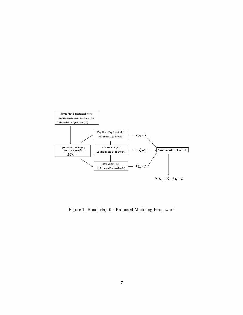
Figure 1: Road Map for Proposed Modeling Framework

7

3 Model of Future Price Expectations

In this section, we describe how a household forms expectations on a brand’s price at a given

period (i.e. shopping trip) in the future. We consider the market for a frequently purchased

product category, and develop the model for an individual household. We will use the subscript

j for a brand in the product category, and the subscript t for a shopping trip of the household.

Our model of future price expectations is based on the following three assumptions: 1.

households expect the price of a brand in each future period to be either a deal price or a

regular price; 2. households know both a brand’s average deal price and average regular price

with certainty; 3. households are uncertain about the temporal occurrence of deals on each

brand (i.e., the likelihood that a deal will occur on a given brand in a given future period).

We use an indicator variable, Ijt+m, to denote whether or not a deal occurs on brand j at

shopping trip t + m, m = 1, 2, ...,. This variable takes the value 1 if a deal occurs on brand j

at trip t + m, and 0 otherwise. We use the notation Prjt+m to denote the probability of deal

occurrence on brand j at trip t + m. This probability is determined by the manufacturer of

brand j or the retailer (in this model, since we are not modeling the interaction between the

manufacturer and the retailer, we do not distinguish between these two decision makers), and

is unobserved by a given household h. Household h, however, “learns” about this probability

on the basis of the values of Ijτ , τ = 1, ..., t that it has observed in the past, i.e., during its

previous shopping trips. In other words, the household forms expectations, at a given trip t,

on the probability Prjt+m on the basis of its shopping experiences in the product category, and

keeps updating these expectations every time it observes a “realization” of Ijτ at the store.

We use the notation EPrhjt+m to denote household h’s expectation of the probability of deal

occurrence on brand j at trip t + m. Given this expectation about deal occurrence, at trip t,

the household arrives at the expected future price of brand j at trip t +m using the following

weighted average:

EPhjt+m = EPrhjt+mPjd + (1 − EPrhjt+m)Pjr, (1)

where Pjd and Pjr stand for the deal price and regular price of brand j respectively (assumed

to be known with certainty by the household).

When household h observes a deal on brand j at trip t, there could be two alternative ef-

8

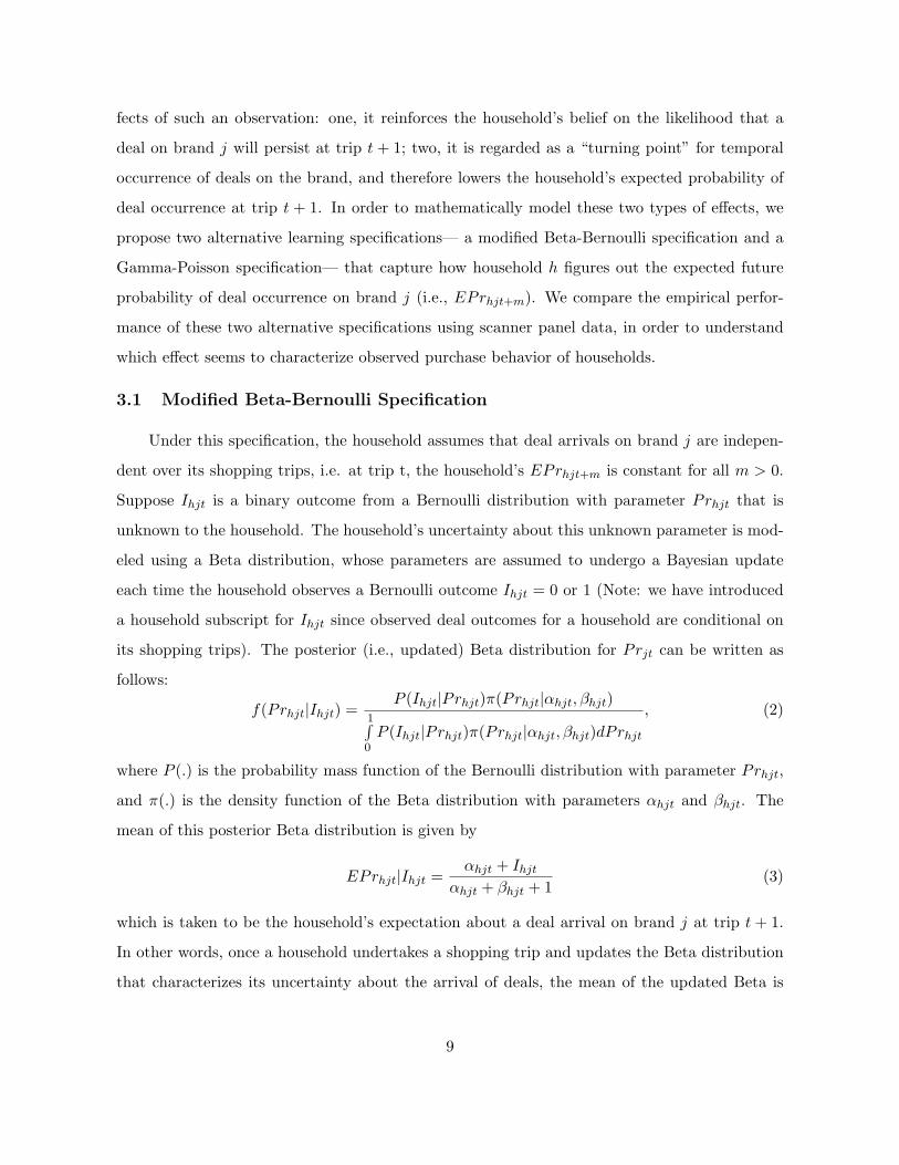
fects of such an observation: one, it reinforces the household’s belief on the likelihood that a

deal on brand j will persist at trip t + 1; two, it is regarded as a “turning point” for temporal

occurrence of deals on the brand, and therefore lowers the household’s expected probability of

deal occurrence at trip t + 1. In order to mathematically model these two types of effects, we

propose two alternative learning specifications— a modified Beta-Bernoulli specification and a

Gamma-Poisson specification— that capture how household h figures out the expected future

probability of deal occurrence on brand j (i.e., EPrhjt+m). We compare the empirical perfor-

mance of these two alternative specifications using scanner panel data, in order to understand

which effect seems to characterize observed purchase behavior of households.

3.1 Modified Beta-Bernoulli Specification

Under this specification, the household assumes that deal arrivals on brand j are indepen-

dent over its shopping trips, i.e. at trip t, the household’s EPrhjt+m is constant for all m > 0.

Suppose Ihjt is a binary outcome from a Bernoulli distribution with parameter Prhjt that is

unknown to the household. The household’s uncertainty about this unknown parameter is mod-

eled using a Beta distribution, whose parameters are assumed to undergo a Bayesian update

each time the household observes a Bernoulli outcome Ihjt = 0 or 1 (Note: we have introduced

a household subscript for Ihjt since observed deal outcomes for a household are conditional on

its shopping trips). The posterior (i.e., updated) Beta distribution for Prjt can be written as

follows:

f(Prhjt|Ihjt) =P (Ihjt|Prhjt)π(Prhjt|αhjt, βhjt)

1∫0P (Ihjt|Prhjt)π(Prhjt|αhjt, βhjt)dPrhjt

, (2)

where P (.) is the probability mass function of the Bernoulli distribution with parameter Prhjt,

and π(.) is the density function of the Beta distribution with parameters αhjt and βhjt. The

mean of this posterior Beta distribution is given by

EPrhjt|Ihjt =αhjt + Ihjt

αhjt + βhjt + 1(3)

which is taken to be the household’s expectation about a deal arrival on brand j at trip t + 1.

In other words, once a household undertakes a shopping trip and updates the Beta distribution

that characterizes its uncertainty about the arrival of deals, the mean of the updated Beta is

9

taken to be the expected probability of deal on brand j during the household’s next shopping

trip. That is, EPrhjt+1 = EPrhjt|Ijt, which yields

EPrhjt+1 =αhjt + Ihjt

αhjt + βhjt + 1=αhj1 + Ihj1 + Ihj2 + ...+ Ihjt

αhj1 + βhj1 + t, (4)

where αhj1 and βhj1 represent the prior parameters of the Beta distribution at t=1, i.e., the first

shopping trip of household h.

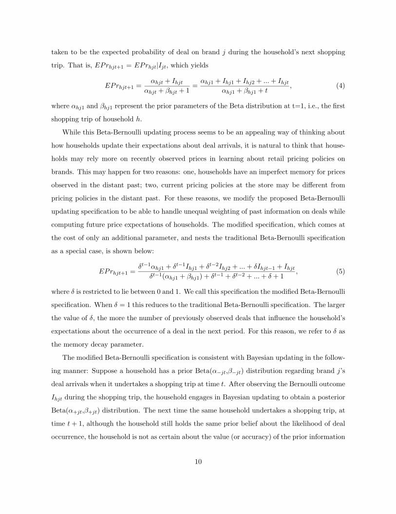
While this Beta-Bernoulli updating process seems to be an appealing way of thinking about

how households update their expectations about deal arrivals, it is natural to think that house-

holds may rely more on recently observed prices in learning about retail pricing policies on

brands. This may happen for two reasons: one, households have an imperfect memory for prices

observed in the distant past; two, current pricing policies at the store may be different from

pricing policies in the distant past. For these reasons, we modify the proposed Beta-Bernoulli

updating specification to be able to handle unequal weighting of past information on deals while

computing future price expectations of households. The modified specification, which comes at

the cost of only an additional parameter, and nests the traditional Beta-Bernoulli specification

as a special case, is shown below:

EPrhjt+1 =δt−1αhj1 + δt−1Ihj1 + δt−2Ihj2 + ...+ δIhjt−1 + Ihjt

δt−1(αhj1 + βhj1) + δt−1 + δt−2 + ...+ δ + 1, (5)

where δ is restricted to lie between 0 and 1. We call this specification the modified Beta-Bernoulli

specification. When δ = 1 this reduces to the traditional Beta-Bernoulli specification. The larger

the value of δ, the more the number of previously observed deals that influence the household’s

expectations about the occurrence of a deal in the next period. For this reason, we refer to δ as

the memory decay parameter.

The modified Beta-Bernoulli specification is consistent with Bayesian updating in the follow-

ing manner: Suppose a household has a prior Beta(α−jt,β−jt) distribution regarding brand j’s

deal arrivals when it undertakes a shopping trip at time t. After observing the Bernoulli outcome

Ihjt during the shopping trip, the household engages in Bayesian updating to obtain a posterior

Beta(α+jt,β+jt) distribution. The next time the same household undertakes a shopping trip, at

time t+ 1, although the household still holds the same prior belief about the likelihood of deal

occurrence, the household is not as certain about the value (or accuracy) of the prior information

10

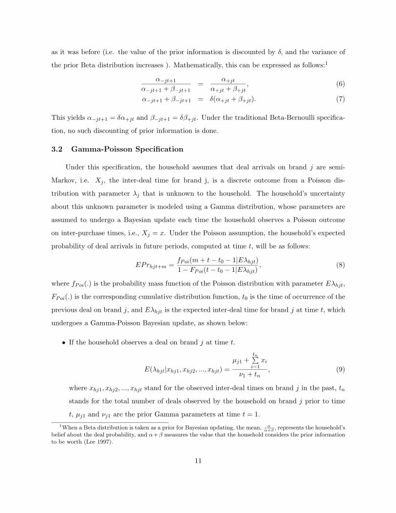
as it was before (i.e. the value of the prior information is discounted by δ, and the variance of

the prior Beta distribution increases ). Mathematically, this can be expressed as follows:1

α−jt+1

α−jt+1 + β−jt+1=

α+jt

α+jt + β+jt, (6)

α−jt+1 + β−jt+1 = δ(α+jt + β+jt). (7)

This yields α−jt+1 = δα+jt and β−jt+1 = δβ+jt. Under the traditional Beta-Bernoulli specifica-

tion, no such discounting of prior information is done.

3.2 Gamma-Poisson Specification

Under this specification, the household assumes that deal arrivals on brand j are semi-

Markov, i.e. Xj , the inter-deal time for brand j, is a discrete outcome from a Poisson dis-

tribution with parameter λj that is unknown to the household. The household’s uncertainty

about this unknown parameter is modeled using a Gamma distribution, whose parameters are

assumed to undergo a Bayesian update each time the household observes a Poisson outcome

on inter-purchase times, i.e., Xj = x. Under the Poisson assumption, the household’s expected

probability of deal arrivals in future periods, computed at time t, will be as follows:

EPrhjt+m =fPoi(m+ t− t0 − 1|Eλhjt)1 − FPoi(t− t0 − 1|Eλhjt)

, (8)

where fPoi(.) is the probability mass function of the Poisson distribution with parameter Eλhjt,

FPoi(.) is the corresponding cumulative distribution function, t0 is the time of occurrence of the

previous deal on brand j, and Eλhjt is the expected inter-deal time for brand j at time t, which

undergoes a Gamma-Poisson Bayesian update, as shown below:

• If the household observes a deal on brand j at time t.

E(λhjt|xhj1, xhj2, ..., xhjt) =µj1 +

tn∑i=1

xi

ν1 + tn, (9)

where xhj1, xhj2, ..., xhjt stand for the observed inter-deal times on brand j in the past, tn

stands for the total number of deals observed by the household on brand j prior to time

t, µj1 and νj1 are the prior Gamma parameters at time t = 1.1When a Beta distribution is taken as a prior for Bayesian updating, the mean, α

α+β, represents the household’s

belief about the deal probability, and α+β measures the value that the household considers the prior informationto be worth (Lee 1997).

11

• If the household does not observe a deal on brand j at time t, Eλhjt remains equal to its

most recent value, i.e., Eλhjt = Eλhjt−1.

It is important to note that our two postulated mechanisms for households’ learning about

future deal occurrences are quite distinct from each other. The modified beta-bernoulli process

says that households assume that future deal occurrences on a brand are independent over

time, which implies that a household’s asking whether or not a deal will occur in the next

period is sufficient from the household’s decision-making standpoint in the current period. The

gamma-poisson process says that households assume that future deal occurrences on a brand are

semi-Markov, which implies that a household ought to consider when the next deal will occur

on each brand in the product category, instead of looking at the next period only. While the

relative empirical merits of these two mechanisms can only be understood using actual purchase

data, one may speculate, a priori, that product categories where deals tend to occur frequently

and with fairly regular periodicity, may be more likely to have households whose future price

expectations follow the gamma-poisson process.

4 Joint Model of Purchase Incidence, Brand Choice and Pur-chase Quantity

In this section, we develop a model of household-level purchase decisions within a given prod-

uct category. Consider a household indexed by h (h = 1, 2, ...,H) observed over t = 1, 2, ..., nh

shopping occasions. On each shopping occasion, we observe a binary outcome variable yht that

takes the value one if the household made a purchase in the focal product category on that

shopping occasion and zero otherwise. This variable captures the household’s “purchase inci-

dence” decision. On those shopping occasions when purchase incidence occurs (i.e. yht is one),

also called purchase occasions, one observes a multinomial outcome variable y∗ht that takes the

value j, j = 1, 2, ..., J , if brand j is bought at that occasion. This variable captures the house-

hold’s “brand choice” decision. For the purchase occasions, one also observes a positive-valued

discrete outcome variable qht that represents the total number of units of brand j bought by

the household. This variable captures the household’s “purchase quantity” decision. Our goal

is to model the outcome variables (yht, y∗ht, qht) on the basis of observed price (Phtj) , display

(Dhtj) and feature (Fhtj) covariates faced by the household at each shopping occasion, and also

12

on the basis of unobserved product inventory and future price expectations of households. Such

a model—called a joint model of purchase incidence, brand choice and purchase quantity—has

been previously developed by Chiang (1991) and Chintagunta (1993). However, these models

ignore the effects of future price expectations. Further, they treat the purchase quantity out-

come as being continuous although observed quantity outcomes are discrete. We address these

two issues and propose a more general econometric model of purchase incidence, brand choice

and purchase quantity, as developed below.

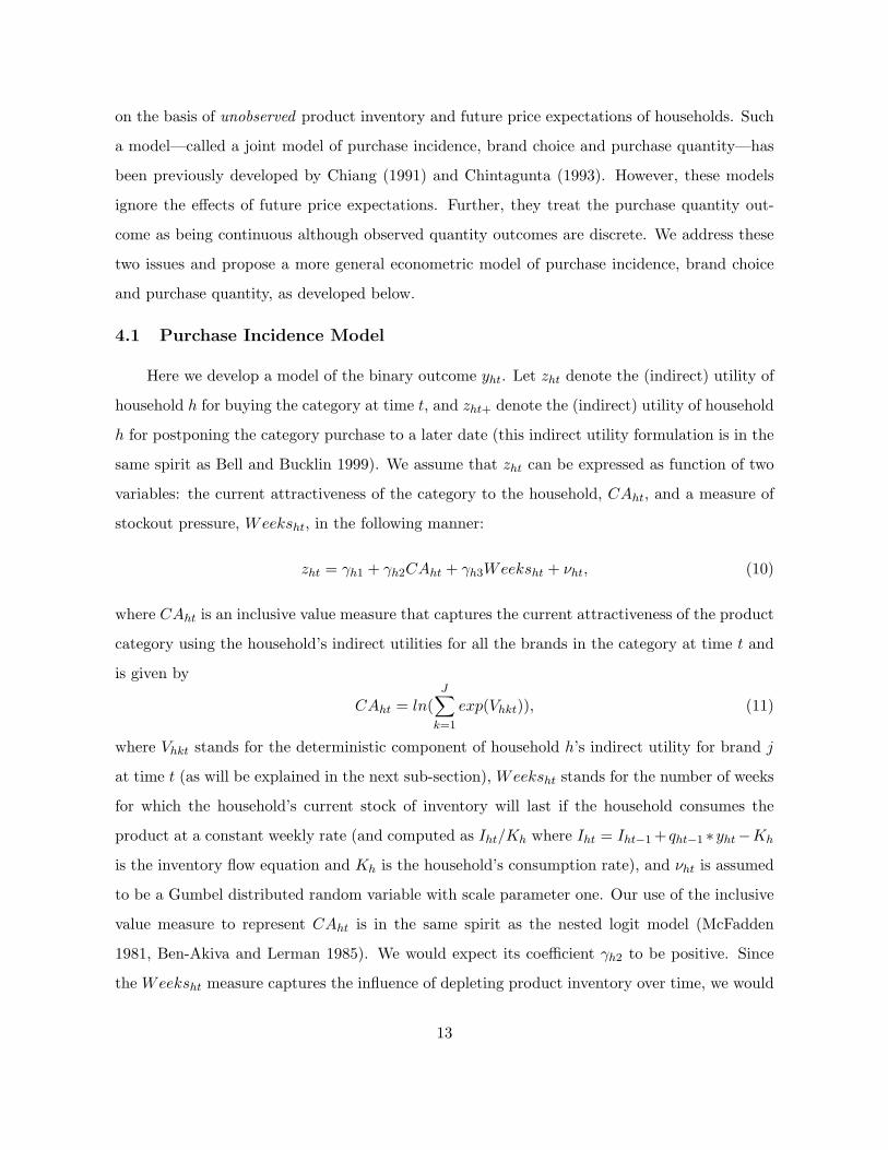
4.1 Purchase Incidence Model

Here we develop a model of the binary outcome yht. Let zht denote the (indirect) utility of

household h for buying the category at time t, and zht+ denote the (indirect) utility of household

h for postponing the category purchase to a later date (this indirect utility formulation is in the

same spirit as Bell and Bucklin 1999). We assume that zht can be expressed as function of two

variables: the current attractiveness of the category to the household, CAht, and a measure of

stockout pressure, Weeksht, in the following manner:

zht = γh1 + γh2CAht + γh3Weeksht + νht, (10)

where CAht is an inclusive value measure that captures the current attractiveness of the product

category using the household’s indirect utilities for all the brands in the category at time t and

is given by

CAht = ln(J∑

k=1

exp(Vhkt)), (11)

where Vhkt stands for the deterministic component of household h’s indirect utility for brand j

at time t (as will be explained in the next sub-section), Weeksht stands for the number of weeks

for which the household’s current stock of inventory will last if the household consumes the

product at a constant weekly rate (and computed as Iht/Kh where Iht = Iht−1 + qht−1 ∗yht−Kh

is the inventory flow equation and Kh is the household’s consumption rate), and νht is assumed

to be a Gumbel distributed random variable with scale parameter one. Our use of the inclusive

value measure to represent CAht is in the same spirit as the nested logit model (McFadden

1981, Ben-Akiva and Lerman 1985). We would expect its coefficient γh2 to be positive. Since

the Weeksht measure captures the influence of depleting product inventory over time, we would

13

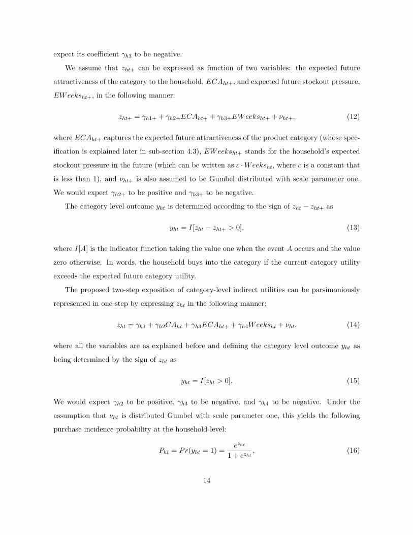
expect its coefficient γh3 to be negative.

We assume that zht+ can be expressed as function of two variables: the expected future

attractiveness of the category to the household, ECAht+, and expected future stockout pressure,

EWeeksht+, in the following manner:

zht+ = γh1+ + γh2+ECAht+ + γh3+EWeeksht+ + νht+, (12)

where ECAht+ captures the expected future attractiveness of the product category (whose spec-

ification is explained later in sub-section 4.3), EWeeksht+ stands for the household’s expected

stockout pressure in the future (which can be written as c ·Weeksht, where c is a constant that

is less than 1), and νht+ is also assumed to be Gumbel distributed with scale parameter one.

We would expect γh2+ to be positive and γh3+ to be negative.

The category level outcome yht is determined according to the sign of zht − zht+ as

yht = I[zht − zht+ > 0], (13)

where I[A] is the indicator function taking the value one when the event A occurs and the value

zero otherwise. In words, the household buys into the category if the current category utility

exceeds the expected future category utility.

The proposed two-step exposition of category-level indirect utilities can be parsimoniously

represented in one step by expressing zht in the following manner:

zht = γh1 + γh2CAht + γh3ECAht+ + γh4Weeksht + νht, (14)

where all the variables are as explained before and defining the category level outcome yht as

being determined by the sign of zht as

yht = I[zht > 0]. (15)

We would expect γh2 to be positive, γh3 to be negative, and γh4 to be negative. Under the

assumption that νht is distributed Gumbel with scale parameter one, this yields the following

purchase incidence probability at the household-level:

Pht = Pr(yht = 1) =ezht

1 + ezht, (16)

14

where γh = (γh1, γh2, γh3, γh4)′ are household-specific coefficients. This is also called the binary

logit model. This is similar to previously proposed binary logit models of purchase incidence

(such as Bucklin and Gupta 1992) except that it includes the influence of expected future

category attractiveness as a covariate in the model.

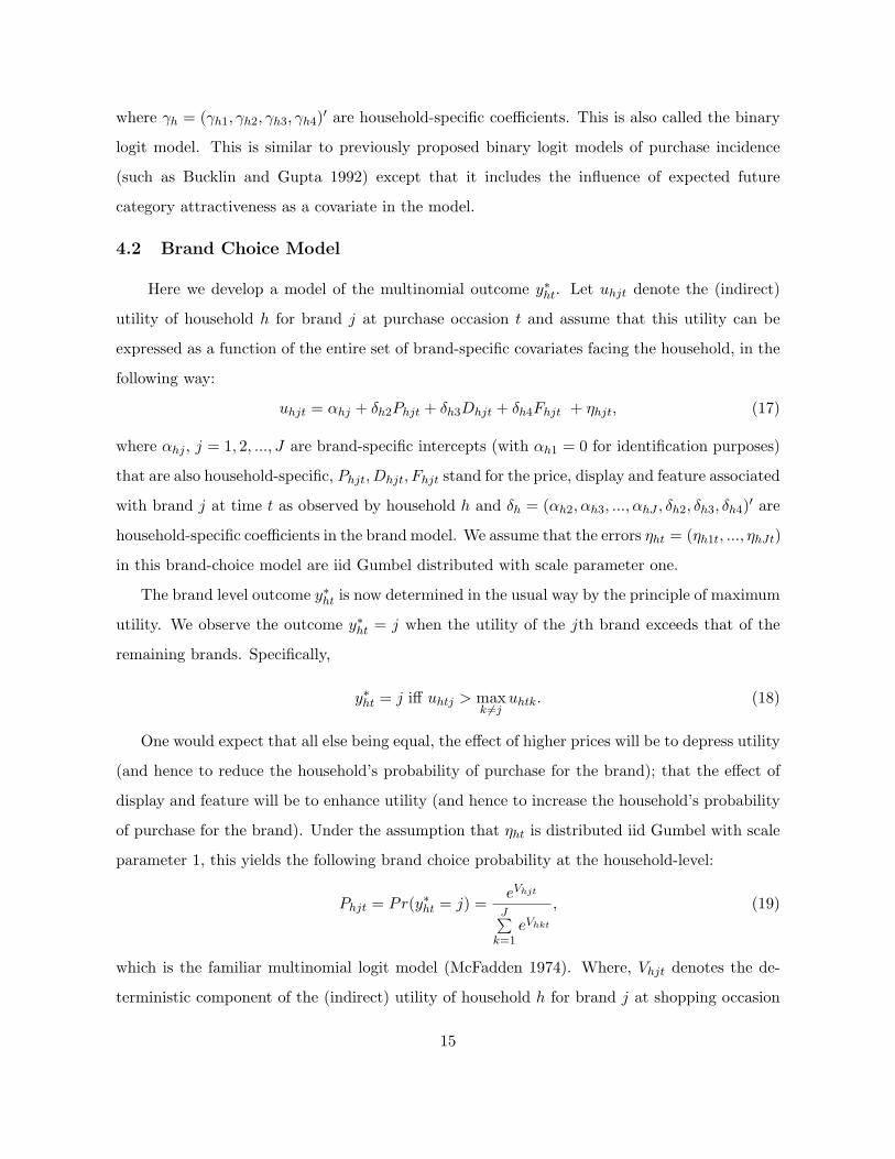
4.2 Brand Choice Model

Here we develop a model of the multinomial outcome y∗ht. Let uhjt denote the (indirect)

utility of household h for brand j at purchase occasion t and assume that this utility can be

expressed as a function of the entire set of brand-specific covariates facing the household, in the

following way:

uhjt = αhj + δh2Phjt + δh3Dhjt + δh4Fhjt + ηhjt, (17)

where αhj , j = 1, 2, ..., J are brand-specific intercepts (with αh1 = 0 for identification purposes)

that are also household-specific, Phjt, Dhjt, Fhjt stand for the price, display and feature associated

with brand j at time t as observed by household h and δh = (αh2, αh3, ..., αhJ , δh2, δh3, δh4)′ are

household-specific coefficients in the brand model. We assume that the errors ηht = (ηh1t, ..., ηhJt)

in this brand-choice model are iid Gumbel distributed with scale parameter one.

The brand level outcome y∗ht is now determined in the usual way by the principle of maximum

utility. We observe the outcome y∗ht = j when the utility of the jth brand exceeds that of the

remaining brands. Specifically,

y∗ht = j iff uhtj > maxk 6=j

uhtk. (18)

One would expect that all else being equal, the effect of higher prices will be to depress utility

(and hence to reduce the household’s probability of purchase for the brand); that the effect of

display and feature will be to enhance utility (and hence to increase the household’s probability

of purchase for the brand). Under the assumption that ηht is distributed iid Gumbel with scale

parameter 1, this yields the following brand choice probability at the household-level:

Phjt = Pr(y∗ht = j) =eVhjt

J∑k=1

eVhkt

, (19)

which is the familiar multinomial logit model (McFadden 1974). Where, Vhjt denotes the de-

terministic component of the (indirect) utility of household h for brand j at shopping occasion

15

t.

Vhjt = αhj + δh2Phjt + δh3Dhjt + δh4Fhjt. (20)

Let EVhjt+m denote the deterministic component of the expected (indirect) utility of house-

hold h for brand j at shopping occasion t+m. Then

EVhjt+m = αhj + δh2EPhjt+m + δh3EDhjt+m + δh4EFhjt+m, (21)

where EPhjt+m, EDhjt+m, EFhjt+m stand for the expected price, display and feature respectively

associated with brand j at time t + m for household h. Since in this study we focus on the

impact of households’ future price expectations, we make a simplification that EDhjt = Dhjt

and EFhjt = Fhjt. This yields

EVhjt+m = αhj + δh2(EPrhjt+mPhjd + (1 − EPrhjt+m)Phjr) + δh3Dhjt+m + δh4Fhjt+m, (22)

which can be rewritten as

EVhjt+m = EPrhjt+mVhjd + (1 − EPrhjt+m)Vhjr, (23)

where

Vhjd = αhj + δh2Phjd + δh3Dhjt + δh4Fhjt, (24)

Vhjr = αhj + δh2Phjr + δh3Dhjt + δh4Fhjt, (25)

where Phjd and Phjr stand for the deal price and regular price associated with brand j respec-

tively.

We then construct a term, the expected future brand utility, EVhjt+, which is the future

counterpart of the deterministic component of the (indirect) utility of household h for brand j

at shopping occasion t, Vhjt. EVhjt+ incorporates household h’s expectations of the brand utility

for the future periods after trip t. It is then computed as shown below:

EVhjt+ = ωjtVhjd + (1 − ωjt)Vhjr. (26)

• For the modified Beta-Bernoulli specification,

ωjt = EPrhjt+1 =δt−1αhj1 + δt−1Ihj1 + δt−2Ihj2 + ...+ δIhjt−1 + Ihjt

δt−1(αhj1 + βhj1) + δt−1 + δt−2 + ...+ δ + t. (27)

16

• For the Gamma-Poisson specification,

ωjt = (1 − γ)∞∑

m=1

γm−1EPrjt+m, (28)

where γ is a time discount factor which lies between 0 and 1.

The appropriate value of EPrjt+m is plugged into this equation based on whether a deal

occurs on brand j at time t or not, and equation (28) can be rewritten as (for details on

the estimable equations, see Zhang 2002):

– If a deal occurs on brand j at t,

ωjt = (1 − γ) exp(−Eλhjt · (1 − γ)), (29)

– If no deal occurs on brand j at t,

ωjt = (1 − γ)

1 + Eλhjt·γy+1 + (Eλhjt·γ)2

(y+1)(y+2) + ...

1 + Eλhjt

y+1 + (Eλhjt)2

(y+1)(y+2) + ...

, (30)

where, y = t− t0 and Eλhjt = Eλhjt−1, as defined before, t0 is the time of occurrence

of the previous deal on brand j.

The current category attractiveness for household h is then expressed as follows:

CAht = ln(J∑

k=1

exp(Vhkt)). (31)

Let ECAht+ denote the expected future category attractiveness. Analogous to the deviation

of CAht, ECAht+ can be computed as shown below:

ECAht+ = ln(J∑

k=1

exp(EVhkt+)). (32)

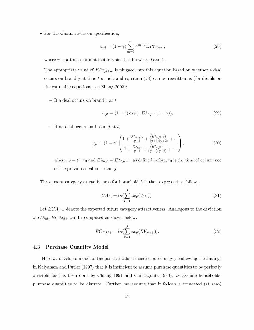
4.3 Purchase Quantity Model

Here we develop a model of the positive-valued discrete outcome qht. Following the findings

in Kalyanam and Putler (1997) that it is inefficient to assume purchase quantities to be perfectly

divisible (as has been done by Chiang 1991 and Chintagunta 1993), we assume households’

purchase quantities to be discrete. Further, we assume that it follows a truncated (at zero)

17

Poisson distribution, i.e., household h’s probability of buying qhjt > 0 units of brand j is given

by

Pr(qhjt = q) =(υhjt)

q

(eυhjt − 1)q!, (33)

where υhjt is a parameter that depends on covariates as shown below:

υhjt = exp (θh1 + θh2Vhjt + θh3ECAhjt+ + θh4(Iht − Ih) + θh5Kh) (34)

and

θh = (θh1, θh2, θh3, θh4, θh5)′

are household-specific coefficients, Ih is household h’s average product inventory over the study

period, Kh is household h’s average product consumption rate, and the remaining variables are

as explained before. We would expect θh2 to be positive, θh3 to be negative, θh4 to be negative,

and θh5 to be positive.

This completes our exposition of our proposed econometric model. It is useful to note here

that we do not allow the household’s brand choice probabilities to depend on the household’s

expected future prices for brands. Since our econometric model is developed under the premise

that the household has an incentive to delay purchase to the future, or to buy reduced quantities

of the product in the current period, on account of its future price expectations, we assume that

the household’s relative preferences for brands are unaffected by future price expectations. It is

mathematically (and statistically) straightforward, however, to extend the brand choice decision

to depend on future price expectations as well. To the extent that the household’s expected

future price for a brand can be viewed as the household’s “reference price” for the brand, our

reference price model is different from previously proposed models in the following manner:

previous models allow the reference price to influence brand choice decisions, while we allow the

reference price to influence the purchase incidence and purchase quantity decisions of households.

4.4 Estimation

Our objective in the empirical section is to estimate the parameters of the joint model

described earlier and to test the effect of future price expectations on purchase incidence and

purchase quantity. To this effect, our objective is to estimate the parameters ψ = (γh, δh, θh)

at the household-level, where γh contains the 4 parameters in the purchase incidence model, δh

18

contains the (J−1)+3 parameters in the brand choice model, and θh contains the 5 parameters

in the purchase quantity model. Assuming the same set of parameters for all households in the

data would yield a total of (J − 1) + 12 estimable parameters. Assuming a discrete random

effects specification for heterogeneity, i.e. S support points whose locations and masses are

flexibly estimated using the data (as in Kamakura and Russell 1989), would yield a total of

S ∗ ((J − 1) + 12) + S − 1 estimable parameters. With five brands (J = 8) and three support-

points (S = 3), for example, we would have 59 estimable parameters.

The likelihood of an observed purchase at the household-level can be written as follows:

Prht = Pr(yht = 1, y∗ht = j, qhjt = q), (35)

and the likelihood of an observed non-purchase at the household-level can be written as follows:

Pr(yht = 0) = 1 − Prht, (36)

which implies that the household-level likelihood function can then be written as

Lh =nh∏t=1

(Prht)yht(1 − Prht)1−yht , (37)

which in turn implies that the sample likelihood function can be written as

L =H∏

h=1

S∑s=1

fsLhs, (38)

where fs is the mass of support point s, and Lhs is household h’s likelihood function computed

using the location of support point s.

One technical concern that arises in this estimation context is the fact that a household’s pur-

chase quantity decision may be correlated, for unobserved reasons, with its purchase incidence

and brand choice decisions. For example, suppose a household buys the product at a shopping

occasion for unobserved reasons—such as the unexpected arrival of guests at home—that are

not explicitly accounted for by the covariates in the purchase incidence model. In such a case,

the household may also be likely to buy a larger quantity of the product for the same unob-

served reasons at that shopping occasion. Unless such a correlation in unobservable is flexibly

accommodated, the parameter estimates of both the purchase incidence model and the purchase

quantity model may be biased. Similarly, suppose the household buys a specific brand of the

19

product at a shopping occasion for unobserved reasons, they may buy a larger quantity of that

brand for the same unobserved reasons. Unless such correlations in unobservable are flexibly

accommodated, the parameter estimates of both the brand choice model and the purchase quan-

tity model may be biased. Such unobserved correlations have been accommodated in previously

proposed models, such as that of Chiang (1991), using the selectivity correction technique of Lee

(1983). However, this technique does not apply when the purchase quantity model is discrete,

as in our case. Therefore, we adapt a recently proposed technique for selectivity bias correction

(Van Ophem 2000), and suitably modify it for our model. This is an important methodological

contribution of this paper, and we describe this next.

Under the assumption of unobserved correlations between a household’s purchase decisions,

the likelihood of an observed purchase at the household-level must be written as follows:

Prht = Pr(yht = 1, y∗ht = j, qhjt = q) = Pr(yht = 1, y∗ht = j, qhjt ≤ q)−Pr(yht = 1, y∗ht = j, qhjt ≤ q−1),

(39)

which can be rewritten as

Prht = N3(Φ−1(Pht),Φ−1(Phjt),Φ−1(Pr(qhjt ≤ q); Σ)

−N3(Φ−1(Pht),Φ−1(Phjt),Φ−1(Pr(qht ≤ q − 1); Σ), (40)

where N3(., ., .; Σ) stands for the cdf of a trivariate normal distribution with covariance matrix

Σ, and Φ(.) stands for the cdf of a standard normal distribution. We assume Σ to be as follows.

Σ =

1 0 ρ13

0 1 ρ23

ρ13 ρ23 1

We ignore unobserved correlations between a household’s purchase incidence and brand

choice decisions (i.e., ρ12 = 0) because the inclusive value measure already captures dependencies

between the two decisions, in the spirit of the nested logit model. However, we estimate the

unobserved correlation between purchase incidence and quantity, ρ13, as well as the vector of

unobserved correlations between brand choice and quantity, ρ23 = (ρ123, ρ223, ..., ρJ23)′, using

a flexible procedure. Under these assumptions the trivariate normal cdf can be conveniently

written as the product of two bivariate normal cdf’s, which substantially simplifies computation

20

since most software packages can evaluate the bivariate cdf directly, which pre-empties the need

for our undertaking numerical simulation (for details on this simplification, see Zhang 2002).

The proposed likelihood function is maximized using gradient-based routines in the SAS/IML

programming environment. The optimal number of support points for the unobserved hetero-

geneity distribution, i.e. S, is identified by sequentially adding supports and re-estimating

model, until there is no further improvement in the Akaike Information Criterion (AIC) of

model fit. This is the commonly used procedure while implementing finite mixture models (see,

for example, Kamakura and Russell 1989).

To reiterate the primary contribution of our proposed model, previously proposed joint

models of purchase incidence, brand choice and purchase quantity—such as Chiang (1991) and

Chintagunta (1993)—ignore the effects of future price expectations on households’ purchase

decisions. A secondary benefit of our framework is that we model purchase quantity as a discrete

outcome, and propose an econometric technique that appropriately corrects for selectivity bias

in its estimates.

5 Description of Data

We employ IRI’s scanner panel database on household purchases in a metropolitan market

in a large U.S. city. For our analysis, we pick the paper towels product category. One reason for

choosing this product category is that, unlike in most other product categories, there is a good

amount of variation (over time and across households) in observed purchase quantities, which

makes the modeling of the household’s purchase quantity (in addition to purchase incidence and

brand choice) decision worthwhile. The dataset covers a period of two years from June 1991 to

June 1993 and contains shopping visit information on 219 panelists across four different stores

in an urban market. The dataset contains information on marketing variables—price, in-store

displays and newspaper feature advertisements—at the SKU-level for each store/week. Since

the single-roll package size accounts for 85 percent of the total quantity sold and 92 percent of all

purchase occasions in this category, and also since eight out of the ten largest-selling brand-size

combinations are of the single-roll type, we focus our attention on this size only.

Choosing households that bought at the largest store in the market more than 80 percent of

the time (since we are not modeling store switching behavior of households), and bought single-

21

roll paper towels on more than 80 percent of their purchase occasions, yields 112 households

making 9902 shopping trips over the study period, among which 1942 are associated with paper

towel purchases. We use the first 70 weeks of data as the calibration sample, and the remaining

34 weeks of data as the validation sample.

There are eight brands in the paper towels category: Private Label, Generic, Bounty, Viva,

Sparkle, Scott, Gala and Mardi Gras. For shopping visits that involve purchase of paper towels,

the marketing variables for the non-purchased brands are computed as share-weighted average

values across all SKUs represented by that brand name. For shopping visits that do not involve

purchase of any paper towels brand, the marketing variables of all brands are computed using

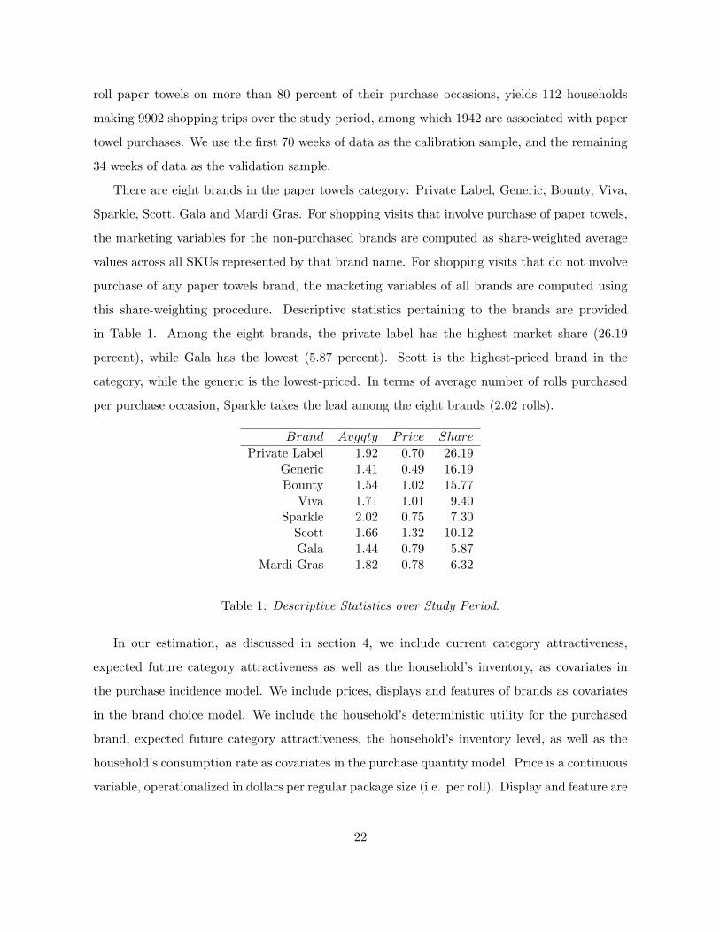
this share-weighting procedure. Descriptive statistics pertaining to the brands are provided

in Table 1. Among the eight brands, the private label has the highest market share (26.19

percent), while Gala has the lowest (5.87 percent). Scott is the highest-priced brand in the

category, while the generic is the lowest-priced. In terms of average number of rolls purchased

per purchase occasion, Sparkle takes the lead among the eight brands (2.02 rolls).

Brand Avgqty Price Share

Private Label 1.92 0.70 26.19Generic 1.41 0.49 16.19Bounty 1.54 1.02 15.77

Viva 1.71 1.01 9.40Sparkle 2.02 0.75 7.30

Scott 1.66 1.32 10.12Gala 1.44 0.79 5.87

Mardi Gras 1.82 0.78 6.32

Table 1: Descriptive Statistics over Study Period.

In our estimation, as discussed in section 4, we include current category attractiveness,

expected future category attractiveness as well as the household’s inventory, as covariates in

the purchase incidence model. We include prices, displays and features of brands as covariates

in the brand choice model. We include the household’s deterministic utility for the purchased

brand, expected future category attractiveness, the household’s inventory level, as well as the

household’s consumption rate as covariates in the purchase quantity model. Price is a continuous

variable, operationalized in dollars per regular package size (i.e. per roll). Display and feature are

22

indicator variables, that take values between 0 and 1, depending on the fraction of SKUs of that

brand that were on display or feature that week. Inventory is a continuous variable (measured

in regular package size), which is computed using the household’s product consumption rate

which, in turn, is computed by dividing the total product quantity purchased by the household

over the study period by the number of weeks in the data. For the first week in the data, each

household is assumed to have enough inventory for that week, i.e. the inventory variable for

a household at t=1 is assumed to be the household’s weekly product consumption rate. Stock

pressure is measured as the household’s existing product inventory divided by the household’s

consumption rate.

6 Empirical Results

We estimate the proposed model under two different specifications of the household’s future

price expectations: modified Beta-Bernoulli and Gamma-Poisson. We will refer to these models

as PROP1 and PROP2 henceforth. We also estimate following benchmark models, which are

nested within the proposed model: 1. model that ignores the effects of future price expectations

(referred to as BENCH1 henceforth), 2. model that ignores the effects of endogenous self-

selectivity in the household’s purchase quantity outcomes (since this model is estimated under

two different specifications for future price expectations, we will refer to them henceforth as

BENCH2A and BENCH2B respectively). Estimating these benchmark models allows us to

investigate the empirical gains from adopting the two modeling innovations inherent in our

proposed model over existing models in the literature.

First, in order to understand the explanatory power of the proposed model vis-a-vis the

benchmark models, we compute the Akaike Information Criterion (AIC) for all models, using

the maximized log-likelihood values (LL) and the following formula: AIC = −2LL+ 2p, where

p stands for the number of parameters in the model. These measures turn out to be -12887 and

-12908 for PROP1 and PROP2 respectively, which indicates that the modified Beta-Bernoulli

specification better explains the observed data than the Gamma-Poisson specification. In other

words, households seem to hold future price-expectations that are consistent with a belief that

brands’ prices arise from a Bernoulli distribution, and are therefore independent over weeks. The

AIC measures based on BENCH1, BENCH2A and BENCH2B turn out to be -12913, -12974

23

and -12998 respectively, which indicates that correcting for endogenous self-selectivity is more

important than accommodating the effects of future price expectations, in terms of improving

the explanatory power of the model. Next, we compute the predictive log-likelihood values for

the holdout sample based on the parameter estimates obtained from the calibration sample.

These measures turn out to be -2417 and -2437 for PROP1 and PROP2 respectively, and -2427,

-2443 and -2436 for BENCH1, BENCH2A and BENCH2B respectively. These validation fits are

quite consistent with the calibration fits noted above.

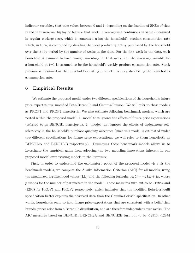
We present the estimated correlations from the matrix Σ of unobserved correlations between

the household’s purchase quantity outcomes, and the household’s purchase incidence and brand

choice outcomes, in Table 2. Under both PROP1 and PROP2, the unobserved correlation

between purchase incidence and purchase quantity is negative. Corresponding to correlations

of -0.28 and -0.30 under PROP1 and PROP2 respectively, this implies that purchase occasions

when households buy paper towels for unobserved reasons are associated with smaller purchase

quantities. This implies that unobserved drivers of paper towels purchases are such that they

do not induce quantity stockpiling in addition to purchase. Explicitly understanding the drivers

of such correlation will be of practical interest to retailers from the standpoint of planning

promotional policies for the paper towels category. The unobserved correlation between brand

choice and purchase quantity is large and positive for the generic brand. Corresponding to

correlations of 0.85 and 0.83 under PROP1 and PROP2 respectively, this implies that purchase

occasions when households buy the generic brand for unobserved reasons are associated with

larger purchase quantities. One possible explanation for this is that when households buy the

generic brand of paper towels for such occasions as home parties, that are unobserved in scanner

panel data, they have to buy a larger quantity of the product as well.

The estimated parameters (and their standard errors) of the purchase incidence model of

PROPOS1 and PROPOS2 are given in Table 3. All the estimated parameters have the expected

signs. Current category attractiveness has coefficients of 2.29 and 2.98 for the two supports under

PROPOS1 (and 1.48 and 1.87 under PROPOS1), while expected future category attractiveness

has corresponding coefficients of −1.03 and −2.51 under PROPOS1 (and −0.24 and −1.48

under PROPOS2). This means that a price cut that increases current category attractiveness

has a positive impact in terms of influencing current purchase, that is larger than the negative

24

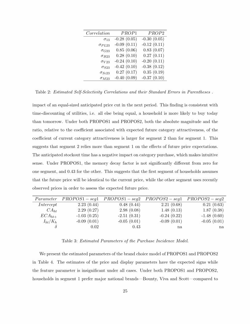
Correlation PROP1 PROP2σ13 -0.28 (0.05) -0.30 (0.05)

σPL23 -0.09 (0.11) -0.12 (0.11)σG23 0.85 (0.06) 0.83 (0.07)σB23 0.28 (0.10) 0.27 (0.11)σV 23 -0.24 (0.10) -0.20 (0.11)σS23 -0.42 (0.10) -0.38 (0.12)σSc23 0.27 (0.17) 0.35 (0.19)σM23 -0.40 (0.09) -0.37 (0.10)

Table 2: Estimated Self-Selectivity Correlations and their Standard Errors in Parentheses .

impact of an equal-sized anticipated price cut in the next period. This finding is consistent with

time-discounting of utilities, i.e. all else being equal, a household is more likely to buy today

than tomorrow. Under both PROPOS1 and PROPOS2, both the absolute magnitude and the

ratio, relative to the coefficient associated with expected future category attractiveness, of the

coefficient of current category attractiveness is larger for segment 2 than for segment 1. This

suggests that segment 2 relies more than segment 1 on the effects of future price expectations.

The anticipated stockout time has a negative impact on category purchase, which makes intuitive

sense. Under PROPOS1, the memory decay factor is not significantly different from zero for

one segment, and 0.43 for the other. This suggests that the first segment of households assumes

that the future price will be identical to the current price, while the other segment uses recently

observed prices in order to assess the expected future price.

Parameter PROPOS1 − seg1 PROPOS1 − seg2 PROPOS2 − seg1 PROPOS2 − seg2Intercept 2.23 (0.44) 0.48 (0.44) 2.21 (0.68) 0.21 (0.63)

CAht 2.29 (0.27) 2.98 (0.08) 1.48 (0.13) 1.87 (0.38)ECAht+ -1.03 (0.25) -2.51 (0.31) -0.24 (0.22) -1.48 (0.60)Iht/Kh -0.09 (0.01) -0.05 (0.01) -0.09 (0.01) -0.05 (0.01)

δ 0.02 0.43 na na

Table 3: Estimated Parameters of the Purchase Incidence Model.

We present the estimated parameters of the brand choice model of PROPOS1 and PROPOS2

in Table 4. The estimates of the price and display parameters have the expected signs while

the feature parameter is insignificant under all cases. Under both PROPOS1 and PROPOS2,

households in segment 1 prefer major national brands—Bounty, Viva and Scott—compared to

25

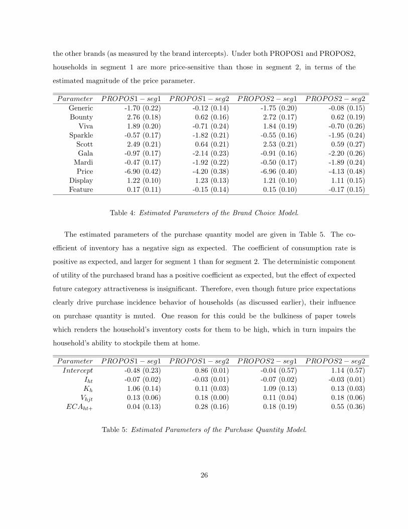
the other brands (as measured by the brand intercepts). Under both PROPOS1 and PROPOS2,

households in segment 1 are more price-sensitive than those in segment 2, in terms of the

estimated magnitude of the price parameter.

Parameter PROPOS1 − seg1 PROPOS1 − seg2 PROPOS2 − seg1 PROPOS2 − seg2Generic -1.70 (0.22) -0.12 (0.14) -1.75 (0.20) -0.08 (0.15)Bounty 2.76 (0.18) 0.62 (0.16) 2.72 (0.17) 0.62 (0.19)

Viva 1.89 (0.20) -0.71 (0.24) 1.84 (0.19) -0.70 (0.26)Sparkle -0.57 (0.17) -1.82 (0.21) -0.55 (0.16) -1.95 (0.24)

Scott 2.49 (0.21) 0.64 (0.21) 2.53 (0.21) 0.59 (0.27)Gala -0.97 (0.17) -2.14 (0.23) -0.91 (0.16) -2.20 (0.26)

Mardi -0.47 (0.17) -1.92 (0.22) -0.50 (0.17) -1.89 (0.24)Price -6.90 (0.42) -4.20 (0.38) -6.96 (0.40) -4.13 (0.48)

Display 1.22 (0.10) 1.23 (0.13) 1.21 (0.10) 1.11 (0.15)Feature 0.17 (0.11) -0.15 (0.14) 0.15 (0.10) -0.17 (0.15)

Table 4: Estimated Parameters of the Brand Choice Model.

The estimated parameters of the purchase quantity model are given in Table 5. The co-

efficient of inventory has a negative sign as expected. The coefficient of consumption rate is

positive as expected, and larger for segment 1 than for segment 2. The deterministic component

of utility of the purchased brand has a positive coefficient as expected, but the effect of expected

future category attractiveness is insignificant. Therefore, even though future price expectations

clearly drive purchase incidence behavior of households (as discussed earlier), their influence

on purchase quantity is muted. One reason for this could be the bulkiness of paper towels

which renders the household’s inventory costs for them to be high, which in turn impairs the

household’s ability to stockpile them at home.

Parameter PROPOS1 − seg1 PROPOS1 − seg2 PROPOS2 − seg1 PROPOS2 − seg2Intercept -0.48 (0.23) 0.86 (0.01) -0.04 (0.57) 1.14 (0.57)

Iht -0.07 (0.02) -0.03 (0.01) -0.07 (0.02) -0.03 (0.01)Kh 1.06 (0.14) 0.11 (0.03) 1.09 (0.13) 0.13 (0.03)Vhjt 0.13 (0.06) 0.18 (0.00) 0.11 (0.04) 0.18 (0.06)

ECAht+ 0.04 (0.13) 0.28 (0.16) 0.18 (0.19) 0.55 (0.36)

Table 5: Estimated Parameters of the Purchase Quantity Model.

26

7 Discussion and Managerial Implications

7.1 Profiling Segments

Given that there are two segments of households that differ in terms of the estimated

parameters of the proposed model, we profile the estimated segments in terms of demographic

and shopping characteristics. In order to do this, we allow each household’s prior probability of

being a member of segment 1 to be a function of demographic and shopping characteristics as

follows:

fhs =eZhb

1 + eZhb, (41)

where Zh is a row-vector of demographic and shopping characteristics characterizing household

h, and bh is the corresponding column-vector of parameters. We include the following variables

in Zh: 1. family size, 2. income (dollars), 3. employment status of female head of household

(=1 if female head works more than 35 hours per week, and 0 otherwise), 4. education of female

head of household (=1 if female head attended college, and 0 otherwise), 5. average purchase

quantity (rolls per purchase occasion), 6. product consumption rate (rolls per week), 7. total

number of shopping trips (i.e. shopping frequency), and 8. total number of purchase occasions

(i.e. purchase frequency). The results of this analysis are given in Table 6. We find that family

size, average purchase quantity and consumption rate all have a positive effect on the household’s

probability of belonging to segment 1. Taken together with our earlier findings that segment

1 is associated with higher price-sensitivity, this suggests that heavy users of paper towels and

larger families are more price-sensitive than light users, which is consistent with previous findings

in the literature (see, for example, Bucklin and Gupta 1992). We also find that employment

status of female head of household, education status of female head of household and shopping

frequency all have a positive effect on the household’s probability of belonging to segment 2.

Taken together with our earlier findings that segment 2 is associated with higher responsiveness

to future deals, this suggests that in order to take advantage of deals, households who shop less

frequently may compensate for their disadvantage of being exposed to fewer deal opportunities

by relying more on future price expectations. Also, more educated and employed consumers

seem to rely more on future prices when they shop.

27

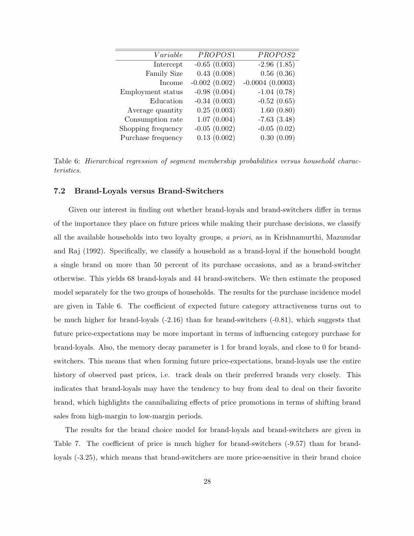
V ariable PROPOS1 PROPOS2Intercept -0.65 (0.003) -2.96 (1.85)

Family Size 0.43 (0.008) 0.56 (0.36)Income -0.002 (0.002) -0.0004 (0.0003)

Employment status -0.98 (0.004) -1.04 (0.78)Education -0.34 (0.003) -0.52 (0.65)

Average quantity 0.25 (0.003) 1.60 (0.80)Consumption rate 1.07 (0.004) -7.63 (3.48)

Shopping frequency -0.05 (0.002) -0.05 (0.02)Purchase frequency 0.13 (0.002) 0.30 (0.09)

Table 6: Hierarchical regression of segment membership probabilities versus household charac-teristics.

7.2 Brand-Loyals versus Brand-Switchers

Given our interest in finding out whether brand-loyals and brand-switchers differ in terms

of the importance they place on future prices while making their purchase decisions, we classify

all the available households into two loyalty groups, a priori, as in Krishnamurthi, Mazumdar

and Raj (1992). Specifically, we classify a household as a brand-loyal if the household bought

a single brand on more than 50 percent of its purchase occasions, and as a brand-switcher

otherwise. This yields 68 brand-loyals and 44 brand-switchers. We then estimate the proposed

model separately for the two groups of households. The results for the purchase incidence model

are given in Table 6. The coefficient of expected future category attractiveness turns out to

be much higher for brand-loyals (-2.16) than for brand-switchers (-0.81), which suggests that

future price-expectations may be more important in terms of influencing category purchase for

brand-loyals. Also, the memory decay parameter is 1 for brand loyals, and close to 0 for brand-

switchers. This means that when forming future price-expectations, brand-loyals use the entire

history of observed past prices, i.e. track deals on their preferred brands very closely. This

indicates that brand-loyals may have the tendency to buy from deal to deal on their favorite

brand, which highlights the cannibalizing effects of price promotions in terms of shifting brand

sales from high-margin to low-margin periods.

The results for the brand choice model for brand-loyals and brand-switchers are given in

Table 7. The coefficient of price is much higher for brand-switchers (-9.57) than for brand-

loyals (-3.25), which means that brand-switchers are more price-sensitive in their brand choice

28

Parameter Loyals Switchers

Intercept -0.44 (0.19) 3.82 (0.70)CAht 2.70 (0.41) 1.70 (0.21)

ECAht+ -2.16 (0.54) -0.81 (0.24)Iht/Kh -0.08 (0.00) -0.10 (0.01)

δ 1.00 (0.07) 0.06(0.06)

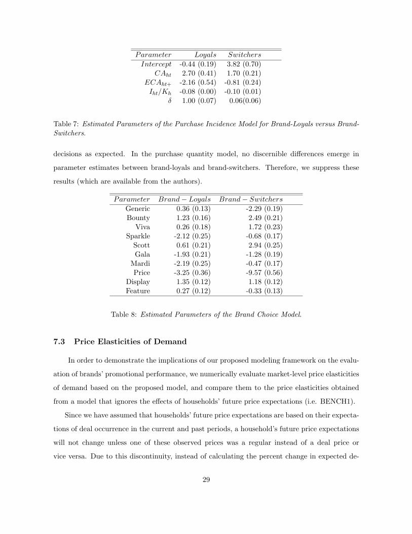
Table 7: Estimated Parameters of the Purchase Incidence Model for Brand-Loyals versus Brand-Switchers.

decisions as expected. In the purchase quantity model, no discernible differences emerge in

parameter estimates between brand-loyals and brand-switchers. Therefore, we suppress these

results (which are available from the authors).

Parameter Brand− Loyals Brand− Switchers

Generic 0.36 (0.13) -2.29 (0.19)Bounty 1.23 (0.16) 2.49 (0.21)

Viva 0.26 (0.18) 1.72 (0.23)Sparkle -2.12 (0.25) -0.68 (0.17)

Scott 0.61 (0.21) 2.94 (0.25)Gala -1.93 (0.21) -1.28 (0.19)

Mardi -2.19 (0.25) -0.47 (0.17)Price -3.25 (0.36) -9.57 (0.56)

Display 1.35 (0.12) 1.18 (0.12)Feature 0.27 (0.12) -0.33 (0.13)

Table 8: Estimated Parameters of the Brand Choice Model.

7.3 Price Elasticities of Demand

In order to demonstrate the implications of our proposed modeling framework on the evalu-

ation of brands’ promotional performance, we numerically evaluate market-level price elasticities

of demand based on the proposed model, and compare them to the price elasticities obtained

from a model that ignores the effects of households’ future price expectations (i.e. BENCH1).

Since we have assumed that households’ future price expectations are based on their expecta-

tions of deal occurrence in the current and past periods, a household’s future price expectations

will not change unless one of these observed prices was a regular instead of a deal price or

vice versa. Due to this discontinuity, instead of calculating the percent change in expected de-

29

mand for a brand when there is a percent change on the brand’s price (as is usually done for

price-elasticity computations), we calculate the change in expected demand when the price of a

brand decreases from the regular price to the deal price. We do this computation based for 100

households who are assumed to have product inventory level, anticipated stock-out time, and

consumption rate equal to the average values computed using all observations in our dataset.

The expected change in demand for brand j within segment s is defined as shown below:

∆E(Qjs) =∞∑

q=1

(Prjqr · q) −∞∑

q=1

(Prjqd · q) , (42)

where Prqr stands for the household’s probability of buying q units of brand j at regular price,

and Prqd stands for the corresponding probability at deal price. The expected change in demand

at the market-level will then be

∆E(Qj) =S∑

s=1

fs∆E(Qj). (43)

Since the proposed model requires the expected future prices of brands, which in turn depend

on prices observed by households in the past, we have to make some assumptions about brand

j’s deal pattern in the past. We use the five most recently observed prices, consider the 25 = 32

possible series of prices in order to calculate the expected change in demand under each case,

and take the average of these 32 values as the expected change in demand. For all brands in the

product category, we find that the benchmark model overstates the effectiveness of promotions.

Specifically, the expected change in demand under the proposed model is smaller than that

under the benchmark model (that ignores future price expectations) by 8 percent for the private

label, 0.3 percent for the generic brand, 17 percent for Bounty, 5 percent for Viva, 10 percent

for Sparkle, 19 percent for Scott, 14 percent for Gala, and 12 percent for Mardi Gras. To the

extent that optimal prices of brands are computed on the basis of estimated price elasticities

of demand, these overstatements have obvious implications for managerial pricing decisions for

brands.

8 Conclusions

We develop a joint econometric model of purchase incidence, brand choice and purchase

quantity decisions at the household-level, that explicitly incorporates the effects of future price

30

expectations of the household. We make two alternative assumptions about the household’s

future price expectations process, both of which are based on the household’s observation (or

lack thereof) of a deal on the current shopping trip: one assumes that the household updates

its belief about the likelihood of deal occurrence on a brand according to a modified Beta-

Bernoulli process; the other assumes that the household updates its belief about a brand’s inter-

deal times according to a Gamma-Poisson process. We embed the household’s expected future

prices, determined according to these updating rules, within the joint econometric model of

the household’s purchase decisions, while explicitly correcting for the effects of endogenous self-

selectivity in the household’s purchase quantity outcomes. Using scanner panel data on paper

towel purchases, we find that the effects of future price expectations are important in terms of

explaining observed purchase incidence outcomes, but not purchase quantity outcomes. We find

that brand-loyals rely more than brand-switchers on the effects of future price expectations. We

also find that infrequent shoppers rely more on the effects of future price expectations, and that

promotional elasticities of demand are overstated if one does not take into account the effects

of future price expectations.

There are some possible areas of future research. First, it will be useful to understand the

cross-category generalizability of our empirical findings by estimating the proposed model on a

wide variety of product categories and noting if cross-category differences emerge. Second, it

would be interesting to investigate whether a given household responds similarly to the effects

of future price expectations across product categories (Seetharaman, Ainslie and Chintagunta

1999). Third, in order to check the robustness of our empirical findings, it will be of value to

estimate alternative econometric models of purchase incidence, such as the proportional haz-

ard model (Seetharaman and Chintagunta 1998), as well as alternative econometric models of

purchase quantity, such as the ordered logit model (Gupta 1988), after including the effects of

future price expectations. Fourth, understanding the competitive promotional implications of

fully specified demand models and the estimated degree of heterogeneity across households in

its parameters will be of value to managers (Narasimhan 1988).

31

References

Bell, D., Bucklin, R. E. (1999). The role of internal reference points in the category purchasedecision. Journal of Consumer Research, 26 (2), 128-143.

Bell, D., Lattin, J. M. (2000). Looking for loss aversion in scanner panel data: The confoundingeffect of price response heterogeneity. Marketing Science, 19 (2), 185-200.

Ben-Akiva, M., Lerman, S. R. (1985). Discrete Choice Analysis. Cambridge, MA: MIT Press.

Bridges, E., Yim, C.K., Briesch, R. A. (1995). A High-Tech Product Market Share Model withCustomer Expectations. Marketing Science, 14 (1), 61-81.

Bucklin, R., Gupta, S. (1992). Brand choice, purchase incidence, and segmentation: An inte-grated modeling approach. Journal of Marketing Research, 16 (2), 201-215.

Chang, K., Siddharth, S., Weinberg, C. B. (1999). The Impact of Heterogeneity in PurchaseTiming and Price Responsiveness on Estimates of Sticker Shock Effects. Marketing Sci-ence, 18 (2), 178-192.

Chiang, J. (1991). A simultaneous approach to the whether, what and how much to buyquestions. Marketing Science, 10 (4), 297-315.

Chintagunta, P. K. (1993). Investigating purchase incidence, brand choice and purchase quan-tity decisions of households. Marketing Science, 12 (2), 184-208.

Coase, R. H. (1972). Durability and Monopoly. Journal of Law and Economics, 12 (2), 184-208.

Cripps, J. D., Meyer, R. J. (1994). Heuristics and biases in timing the replacement of durableproducts. Journal Of Consumer Research, 21 (2), 304-318.

Deaton, A., Muellbauer, J. (1980). Economics and Consumer Behavior. Cambridge, MA:Cambridge University Press.

Erdem, T., Mayhew, G., Sun, B. (2001). Understanding the reference price shopper: A withinand cross-category analysis. Journal of Marketing Research, 38 (4), 445-457.

Erdem, T., Imai, S., Keane, M. P. (2002). Consumer price and promotion expectations: Cap-turing consumer brand and quantity choice dynamics under price uncertainty. Workingpaper, University of California at Berkeley.

Gonul, F., Srinivasan, K. (1996). Estimating the impact of consumer expectations of couponson purchase behavior: A dynamic structural model. Marketing Science, 15(3), 262-278.

Gupta, S. (1988). Impact of sales promotions on when, what, and how much to buy. Journalof Marketing Research, 25(4), 342-355.

Hannemann, W. M (1984). Discrete/continuous models of consumer demand. Econometrica,52, 541-561.

32

Jacobson, R., Obermiller, C. (1990). The formation of expected future price: A reference pricefor forward-looking consumers. Journal of Consumer Research, 16 (March), 420-431.

Kalyanam, K., Putler, D. S. (1997). Incorporating demographic variables in brand choicemodels: An indivisible alternatives framework. Marketing Science, 16(2), 166-181.

Kamakura, W. A., Russell, G. J. (1989). A probabilistic choice model for market segmentationand elasticity structure. Journal of Marketing Research, 26(4), 379-390.

Krishna, A. (1992). The normative impact of consumer price expectations for multiple brandson consumer purchase behavior. Marketing Science, 11 (3), 266–286.

Krishnumurthi, L., Mazumdar, T., Raj, S. P. (1992). Asymmetric response to price in consumerchoice and purchase quantity decisions. Journal of Consumer Research, 19 (December),387-400.

Lee, L. F. (1983). Generalized econometric models with selectivity. Econometrica, 51, 507-512.

Lee, P. M. (1997). Bayesian Statistics: An Introduction. John Wiley & Sons Inc.

McFadden, D. (1974). Conditional logit analysis in qualitative choice behavior. In Zarembka,P. Frontiers in Econometrics. New York: Academic Press, 105-142.

McFadden, D. (1981). Econometric models of probabilistic choices. In Manski, C. F., Mc-Fadden, D. (Eds.). Structure Analysis of Discrete Data with Econometric Applications.Cambridge, MA: MIT Press.

Meyer, R. J., Assuncao, J. (1990). The optimality of consumer stockpiling strategies. Market-ing Science, 9 (1), 18-41.

Meyer, R. J., Shi, Y. (1995). Sequential choice under ambiguity: Intuitive solutions to thearmed-bandit problem. Management Science, 41 (5), 817-834.

Narasimhan, C. (1988). Competitive promotional strategies. Journal of Business, October,427-50.

Narasimhan, C. (1989). Incorporating Consumer Price Expectations in Diffusion Models. Mar-keting Science, 8 (4), 343-357.

Narasimhan, C., Neslin, Scott A., Sen, S. K. (1996). Promotional elasticities and categorycharacteristics. Journal of Marketing, 60 (2), 17-30.

Seetharaman, P. B., Chintagunta, P. K. (2002). The Proportional Hazard Model for PurchaseTiming: A Comparison of Alternative Specifications. Journal of Business and EconomicStatistics, forthcoming.

Seetharaman, P. B., Ainslie, A. K., Chintagunta, P. K. (1999). Investigating household statedependence effects across categories. Journal of Marketing Research, 36 (4), 488-500.

Stokey, N. L. (1981). Rational Expectations and Durable Goods Pricing. The Bell Journal ofEconomics, 12 (1), 112-128.

33

Sun, B. (2002). Promotion effects on category sales with endogenized consumption and pro-motion uncertainty. Working paper, Carnegie Mellon University.

Van Ophem, H. (2000). Modeling selectivity in count-data models. Journal of Business andEconomic Statistics, 18 (4), 503-511.

Winer, R.S. (1985). A Price Vector Model of Demand for Consumer Durables. MarketingScience, 4 (1), 74-90.

Winer, R.S. (1986). A Reference Price Model of Brand Choice for Frequently PurchasedProducts. Journal of Consumer Research, 13 (2), 250-256.

Zhang, Q. (2002). Incorporating Future Price Expectations into Consumer Purchase Deci-sions. Unpublished doctoral dissertation, John M. Olin School of Business, WashingtonUniversity, St. Louis, MO 63130.

34