Incorporating lifecycle and environment in

loan-level forecasts and stress tests

Joseph L BreedenPrescient Models LLC300 Catron St., Suite B

Santa Fe, NM 87501, USAbreeden@prescientmodels.com

+1 505-490-6042

July 21, 2014

Abstract

The new FASB current expected credit loss (CECL) proposal, IASB’sIFRS 9, and regulatory stress testing all require that the industry movetoward forecasting probabilities of future events, rather than simply rank-ordering loans. Even more importantly, effective loan pricing requires thissame forward-looking, loan-level forecasting.

We created a loan-level version of Age-Period-Cohort (APC) modelssuitable for forecasting individual loan performance at a point-in-time orfor the loan’s lifetime. The APC literature explains that any model of loanperformance must make either an explicit or implicit assumption aroundthe embedded model specification error between age of the loan, vintageorigination date, and performance date. We have made this assumptionexplicit and implemented a technique using augmented macroeconomichistory to stabilize the analysis.

The preceding steps provide robust estimates of lifecycle and environ-mental impacts. We then use a Generalized Linear Model (GLM) with apopulation odds offset for each age / time combination derived from thelifecycle and environment functions in order to estimate origination andbehavior scores. Analyzing a small US auto loan portfolio, we demonstratethat this model is robust out-of-sample and out-of-time for predicting bothrank-ordering and probabilities by inserting the odds offset appropriatefor the environment being modeled.

In addition to producing loan-level forecasts and stress tests, the scoresproduced have higher rank-order performance out-of-sample and out-of-time than standard scores. The scores prove to be robust years into thefuture with no measurable degradation in performance because of thestabilizing effect of the offset factor during model construction.

Keywords: Forecasting; Risk, Banking; Time series; Age-Period-CohortModels

1

2

1 Introduction

Credit scores were originally developed to aid loan origination. Applicants wouldbe screened by estimating a score from available application data. The scoreserved as an impartial criterion for assessing risk. The “cut-off” score was thethreshold below which riskier applicants were denied loans.

The transition to risk-based pricing meant that a wider range of applicantscould be accepted by modifying the loan terms to match the riskiness of theapplicant. Risk-based pricing came in response to competitive pressure amonglenders. As margins contracted, lenders needed to better target their pricing.

As lenders became more reliant on scores, greater effort was put into im-proving score accuracy. Improved estimation techniques, the transition to logitand probit models, and the use of bureau attributes all enhanced the ability ofthe scores to assess risk.

The scorecard uses these factors from a dataset, x, to predict the probabilityof “good”, p(G|x). The odds of a loan being good are [12]

o(G|x) =p(G|x)

p(B|x)=pGpB

p(x|G)

p(x|B)≡ oPop × I(x),x ∈ X (1)

orlog(o(G|x)) ≡ log(oPop) + log(I(x)) (2)

where pG and pB are the unconditional odds of good or bad, pG

pBis the population

odds oPop, and I(x) = p(x|G)p(x|B) is the information odds. We could also say

that oPop captures systematic effects for the portfolio and I(x) captures theidiosyncratic effects for an individual loan.

When we create a credit score, we expect the information odds to be reason-ably robust out-of-sample. The population odds, however, are dependent uponthe macroeconomic conditions prevailing during the in-sample period. In futuretime periods, the population odds should change due to factors not capturedin the credit score. For this reason, credit scores are used as risk ranking toolsout-of-time, not as predictors of o(G|xoot) where xoot are the loan attributesout-of-time. (Out-of-time refers to data from time periods not included in thetraining sample.)

Many practitioners expand the attributes x to include macroeconomic fac-tors and the age of the loan in an attempt to predict the population odds aswell, but with mixed results. As explained in the Age-Period-Cohort (APC)literature [10, 7] and applied to the context of credit risk modeling [3], a modelspecification error is embedded in the dynamics of retail lending. Traditionalcredit scoring attributes are measured in the loan origination month, also knownas the vintage date, v. Macroeconomic data is measured with calendar date t.Lifecycle functions as in survival models [4, 8, 11, 6] are measured versus theage of the loan a. However, a = t − v, leading to a linear specification error iffactors measured along all three dimensions are included in the model simulta-neously and without constraint. In cases where some of these dimensions areexcluded, as with traditional credit scores that rely solely on information from

3

the origination (vintage) date, a unique solution is obtained, but at the cost ofbeing unable to predict probabilities in future time periods.

The APC literature proves that no general solution exists for this specifica-tion error, with the implication that we can never be certain of the linear trendsin lifecycle, macroeconomic, or credit risk functions. Instead, domain-specificsolutions are recommended by incorporating constraints suitable to the specificsituation being modeled. An inability to be certain of linear trends in timewould me that we could not reliably predict the population odds in future timeperiods, brining the effectiveness of any stress test model into question.

Breeden and Thomas [3] described a constraint that would appear to bereasonable for retail lending. Namely, that after fitting macroeconomic factorsto the environment function, the slope of that macroeconomic impact shouldbe zero when extrapolated backward across multiple macroeconomic cycles. Forany model that includes macroeconomic factors, this is equivalent to creating anenvironmental index from a subset of the model as E = f(Ei(t), ci) where the Ei

are the individual macroeconomic factors and ci are the estimated coefficientsfor their inclusion in the credit risk model. Then create the constraint thatslope(E(t)) = 0 when E(t) is extrapolated backward over multiple decades ofmacroeconomic history.

Over any short time frame of less than one economic cycle, the environmentwill certainly not show zero trend, but the assumption of zero trend over manycycles is consistent with the assumption that a through-the-cycle average canbe defined for macroeconomic impacts, i.e. that a through-the-cycle probabilityof default (PD) exists in the sense that the population odds can be a constantwhen measured for a reference portfolio across multiple economic cycles..

Using the technique of Breeden and Thomas to control the model specifi-cation error, we demonstrate a method of creating credit scores that estimatesboth the population odds and information odds in-sample, and provides for ex-trapolating the population odds out-of-sample so that loan-level probabilitiesare forecasted.

2 Modeling approach

Although a single-stage approach is in principle possible using a constrainedoptimization, we followed a sequential analysis using simpler algorithms. Thefollowing steps were performed in the analysis.

1. Decompose loan-level performance data with an Age-Vintage-Time (AVT)

2. Fit the time function to macroeconomic data

3. Retrend the age and vintage functions

4. Fit a credit score with age and time offsets

4

2.1 Age-Vintage-Time decomposition

The first step is to estimate the lifecycle as a function of age of the loan, thevintage quality as a function of vintage, and the environment as a function oftime (calendar date). This analysis should be performed on the longest historyavailable, preferably longer than the two to three years of history that is typicalof credit scores.

For the Age-Vintage-Time (AVT) decomposition, we can use standard Age-Period-Cohort (APC) implementations to analyze vintage-aggregate time serieswith a logit transformation, or use an equivalent loan-level implementation ofAPC. Each vintage will be measured each month to create an appropriate rate.For example, to predict the default rate, default accounts and active accountswould be reported each month. The APC algorithm would estimate

r(a, v, t) =Defaults(t)

Active.Accounts(t− 1)=

1

1 + e−(F (a)+G(v)+H(t))(3)

where r(a, v, t) is the default rate, F (a) is the lifecycle with age, G(v) isthe credit quality by vintage, and H(t) is the environment function over time.With standard implementations of the APC algorithm, all three functions areestimated via splines with the analyst specifying the number of spline nodes.Although F (a) is usually given fewer nodes on the assumption of a relativelysmooth lifecycle function, G(v) and H(t) should have as many nodes as thedata will support in order to capture sudden changes in the portfolio composi-tion or macroeconomic environment respectively. Alternatively, standard APCimplementations usually support nonparameteric estimation of any of the threefunctions.

For loan-level data, we created an implementation equivalent to the APC al-gorithm. Although we can use a range of distributions and link functions, a logittransform is again desirable to model default rate. The loan-level data will con-tain periodic observations of each account until default or voluntary attrition.Each observation will report a binary value for default. After default or volun-tary attrition, the loan is no longer reported. In a loan-level analysis, reportingonly active loans is equivalent to using active accounts as the denominator ofthe aggregate rate modeling in Equation 3.

logit(pi(a, v, t)) = F (a) +G(v) +H(t) (4)

With the loan-level AVT algorithm, the same spline approximations wereavailable, but nonparametric estimation of any of the functions is also availableassuming sufficient data exists to estimate all the coefficients.

Note that the loan-level estimation of Equation 4 still results in population-wide functions of F (a), G(v), and H(t). In fact, aside from estimation errors,both approaches will estimate the same functions on a given data set. Thesefunctions essentially capture the population odds in-sample. To predict the pop-ulation odds out-of-sample, we need to extrapolate H(t) for future environmentsand move all the loans along the lifecycle function F (a) as they age. Since these

5

functions are designed to capture all of the systematic effects in the portfolio,the remaining structure should be loan-level idiosyncratic effects, as found inthe information odds.

2.2 Macroeconomic fit

The environmental function H(t) is initially estimated with the assumptionof no net trend with time over the observed portfolio data. As the data isfit to macroeconomic data, the no-trend constraint is relaxed in order to findthe best fit to available macroeconomic factors. To avoid overfitting, we onlyconsider factors that are close to the consumer balance sheet: employment /unemployment / under-employment; house prices; real wages; interest rates,etc.

In each of these cases, careful consideration must be given to the transforma-tions used. Since a logit transformation is used in Equation 4, the H(t) functionwill be roughly normally distributed. Any explanatory macroeconomic factorsshould be transformed to be roughly normally distributed as well. For example,the house price index (HPI) is usually reported as year-over-year percentagechange. Although intuitively useful, percentage change is asymmetric. A 10%period-over-period increase followed by a 10% decrease does not return the indexto its original value. Instead, we borrow from the investment analytics worldto select transformations that are symmetric and approximately normally dis-tributed so that linear regression may be employed. A table of preferred trans-formations maybe be found in Breeden (2010) [1]. For changes in HPI, we shoulduse a log-ratio transformation, log − ratio(HPI) = log(HPI(t)/HPI(t − w)where w is the window over which the change is computed.

Once a transformation has been chosen, we consider lags and moving aver-ages of the transformed values. This is equivalent to a simplified DistributedLag Model [9]. The lags and moving averages become part of the transformationof the macroeconomic variable prior to creating the final regression model. Ifseveral variables are found that contain predictive power, we will attempt tocreate a multiple regression model,

H(t) = c0t+∑i

ciEi(t) + εt, (5)

where c0 is the linear trend coefficient, ci are the coefficients against transformedmacroeconomic factors Ei(t), εt ∈ N (0, σ) and t spans the date range of theobserved portfolio performance data, t ∈ [0, To]. The process of fitting the envi-ronmental function to macroeconomic data has been previously demonstratedfor APC-class models [2, 3].

2.3 Retrending the functions

Using the technique of Breeden and Thomas [3], the fitted environmental func-tion H(t) is extrapolated backward through previous economic cycles [−Th, 0)

6

not represented in the portfolio performance data. A straight line is fit throughthe extrapolation of H(t) over the range t ∈ [−Th, To] as H(t) = α+ βt.

The original lifecycle, vintage quality, and time functions are retrended as

F ′(a) = F (a) + βa

G′(v) = G(v) + βv (6)

H ′(t) = H(t)− βt

Retrending can also be performed by rerunning the AVT estimation with theretrended H ′(t) as a fixed input. The estimated F ′(a) and G′(v) will preservethe original data density weighting and is generally the easiest approach toguarantee the functions are optimized to the data.

Retrending these functions by leveraging a greater macroeconomic historyprovides a reasonable solution to the extrapolation problem. Many forecast orstress test models trend strongly upward or downward into the distant futurebecause of the uncontrolled or unobserved trend acquired during initial mod-eling. By detrending over multiple economic cycles, we create a model that isstationary and consistent with the philosophy that a long-run PD exists andcan be modeled. Simply subtracting off the linear trend is reasonable, since theassigned linear trend was arbitrary in the original estimation.

2.4 Fitting the Score

The final modeling step is to use the retrended lifecycle and environment func-tions to compute the monthly populations odds as a function of the age of theloan and macroeconomic environment. This is referred to as the offset(a, t) =F ′(a) +H ′(t) where H ′(t) is the detrended fit to macroeconomic data.

With this, a scoring function is created to predict defaults as a function oftypical scoring attributes X,

logit(pi(a, t)) = offset(a, t) + BX, (7)

where B are the score coefficients. The offset is equivalent to an attribute witha fixed coefficient of 1. The coefficients are estimated via a generalized linearmodel (GLM) on a loan-level data matrix of monthly performance observations.

3 Numerical Example

This process was tested on a small US auto loan portfolio. Historic loan-levelperformance data was available from 2004 through 2012 for all vintages duringthat period. The monthly default rate was modeled

DR(a, v, t) =Default Accounts(t)

Active Accounts(t− 1)(8)

The steps described in Section 2 were followed.

7

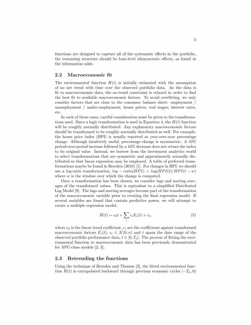
3.1 AVT Analysis

Using a loan-level implementation of Age-Period-Cohort models with an initialassumption that the environment function had no trend over the in-sample dataprovided the following results.

0 12 24 36 48 60 72 84 96 108

0.00

00.

001

0.00

20.

003

0.00

4

Small Auto Loan Portfolio

Age

Life

cycl

e Fu

nctio

n

Figure 1: Lifecycle function with account age measured for a small US autoloan portfolio

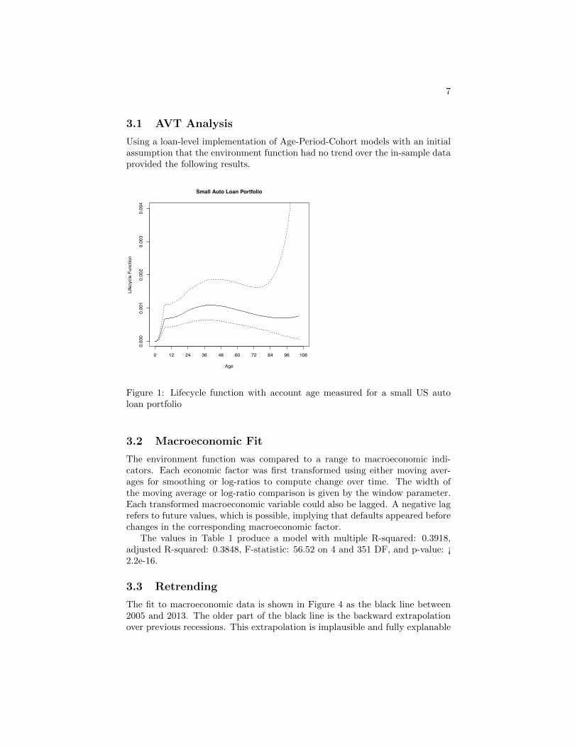
3.2 Macroeconomic Fit

The environment function was compared to a range to macroeconomic indi-cators. Each economic factor was first transformed using either moving aver-ages for smoothing or log-ratios to compute change over time. The width ofthe moving average or log-ratio comparison is given by the window parameter.Each transformed macroeconomic variable could also be lagged. A negative lagrefers to future values, which is possible, implying that defaults appeared beforechanges in the corresponding macroeconomic factor.

The values in Table 1 produce a model with multiple R-squared: 0.3918,adjusted R-squared: 0.3848, F-statistic: 56.52 on 4 and 351 DF, and p-value: ¡2.2e-16.

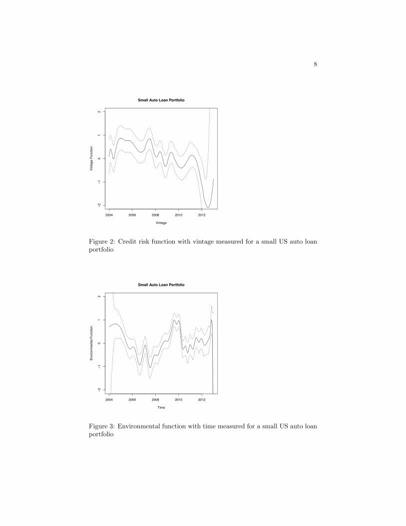
3.3 Retrending

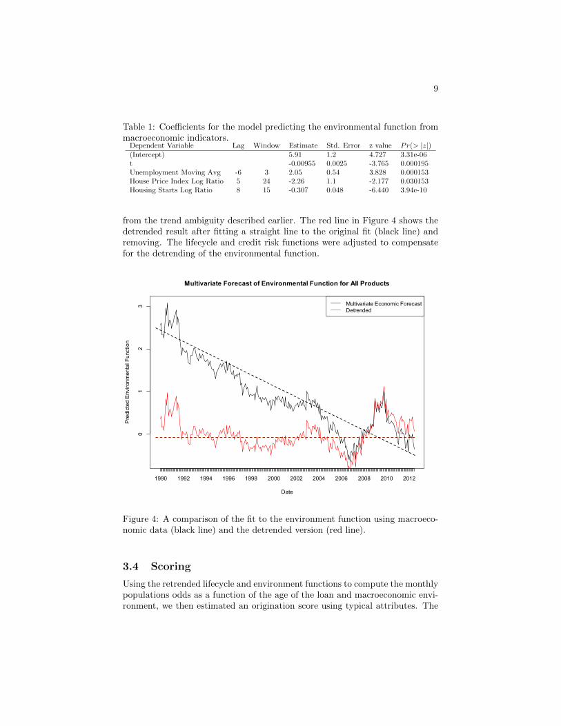
The fit to macroeconomic data is shown in Figure 4 as the black line between2005 and 2013. The older part of the black line is the backward extrapolationover previous recessions. This extrapolation is implausible and fully explanable

8

2004 2006 2008 2010 2012

−2−1

01

2Small Auto Loan Portfolio

Vintage

Vint

age

Func

tion

Figure 2: Credit risk function with vintage measured for a small US auto loanportfolio

2004 2006 2008 2010 2012

−2−1

01

2

Small Auto Loan Portfolio

Time

Envi

ronm

enta

l Fun

ctio

n

Figure 3: Environmental function with time measured for a small US auto loanportfolio

9

Table 1: Coefficients for the model predicting the environmental function frommacroeconomic indicators.

Dependent Variable Lag Window Estimate Std. Error z value Pr(> |z|)(Intercept) 5.91 1.2 4.727 3.31e-06t -0.00955 0.0025 -3.765 0.000195Unemployment Moving Avg -6 3 2.05 0.54 3.828 0.000153House Price Index Log Ratio 5 24 -2.26 1.1 -2.177 0.030153Housing Starts Log Ratio 8 15 -0.307 0.048 -6.440 3.94e-10

from the trend ambiguity described earlier. The red line in Figure 4 shows thedetrended result after fitting a straight line to the original fit (black line) andremoving. The lifecycle and credit risk functions were adjusted to compensatefor the detrending of the environmental function.

1990 1992 1994 1996 1998 2000 2002 2004 2006 2008 2010 2012

01

23

Multivariate Forecast of Environmental Function for All Products

Date

Pre

dict

ed E

nviro

nmen

tal F

unct

ion

Multivariate Economic ForecastDetrended

Figure 4: A comparison of the fit to the environment function using macroeco-nomic data (black line) and the detrended version (red line).

3.4 Scoring

Using the retrended lifecycle and environment functions to compute the monthlypopulations odds as a function of the age of the loan and macroeconomic envi-ronment, we then estimated an origination score using typical attributes. The

10

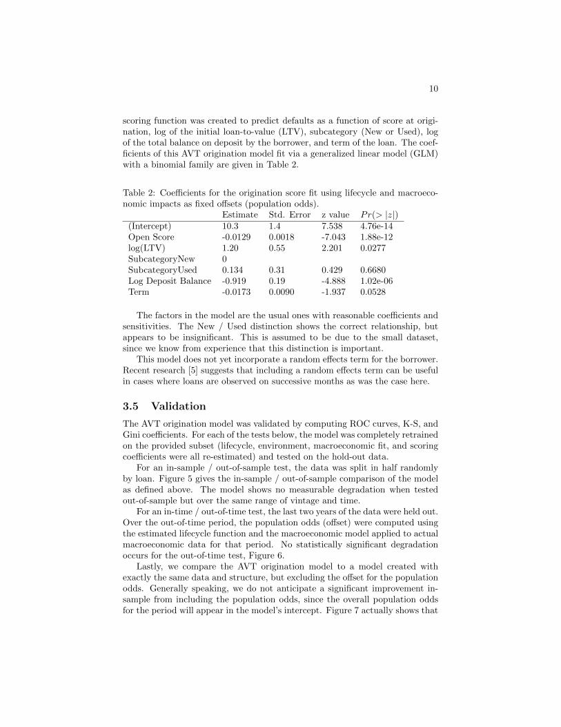
scoring function was created to predict defaults as a function of score at origi-nation, log of the initial loan-to-value (LTV), subcategory (New or Used), logof the total balance on deposit by the borrower, and term of the loan. The coef-ficients of this AVT origination model fit via a generalized linear model (GLM)with a binomial family are given in Table 2.

Table 2: Coefficients for the origination score fit using lifecycle and macroeco-nomic impacts as fixed offsets (population odds).

Estimate Std. Error z value Pr(> |z|)(Intercept) 10.3 1.4 7.538 4.76e-14Open Score -0.0129 0.0018 -7.043 1.88e-12log(LTV) 1.20 0.55 2.201 0.0277SubcategoryNew 0SubcategoryUsed 0.134 0.31 0.429 0.6680Log Deposit Balance -0.919 0.19 -4.888 1.02e-06Term -0.0173 0.0090 -1.937 0.0528

The factors in the model are the usual ones with reasonable coefficients andsensitivities. The New / Used distinction shows the correct relationship, butappears to be insignificant. This is assumed to be due to the small dataset,since we know from experience that this distinction is important.

This model does not yet incorporate a random effects term for the borrower.Recent research [5] suggests that including a random effects term can be usefulin cases where loans are observed on successive months as was the case here.

3.5 Validation

The AVT origination model was validated by computing ROC curves, K-S, andGini coefficients. For each of the tests below, the model was completely retrainedon the provided subset (lifecycle, environment, macroeconomic fit, and scoringcoefficients were all re-estimated) and tested on the hold-out data.

For an in-sample / out-of-sample test, the data was split in half randomlyby loan. Figure 5 gives the in-sample / out-of-sample comparison of the modelas defined above. The model shows no measurable degradation when testedout-of-sample but over the same range of vintage and time.

For an in-time / out-of-time test, the last two years of the data were held out.Over the out-of-time period, the population odds (offset) were computed usingthe estimated lifecycle function and the macroeconomic model applied to actualmacroeconomic data for that period. No statistically significant degradationoccurs for the out-of-time test, Figure 6.

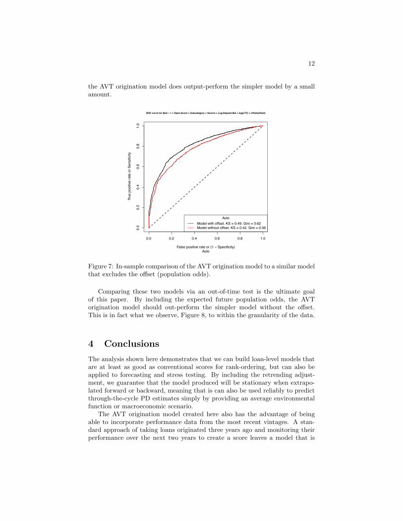
Lastly, we compare the AVT origination model to a model created withexactly the same data and structure, but excluding the offset for the populationodds. Generally speaking, we do not anticipate a significant improvement in-sample from including the population odds, since the overall population oddsfor the period will appear in the model’s intercept. Figure 7 actually shows that

11

0.0 0.2 0.4 0.6 0.8 1.0

0.0

0.2

0.4

0.6

0.8

1.0

False positive rate or (1 − Specificity)

Tru

e po

sitiv

e ra

te o

r Sen

sitiv

ity

ROC curve for Bad ~ 1 + Open.Score + Subcategory + Source + Log.Deposit.Bal + log(LTV) + offset(offset)

Auto

AutoOut−of−Sample. KS = 0.49. Gini = 0.62In−Sample. KS = 0.5. Gini = 0.63

Figure 5: The AVT origination model was trained on half the data randomlysampled by loan and tested on the excluded half.

0.0 0.2 0.4 0.6 0.8 1.0

0.0

0.2

0.4

0.6

0.8

1.0

False positive rate or (1 − Specificity)

Tru

e po

sitiv

e ra

te o

r Sen

sitiv

ity

ROC curve for Bad ~ 1 + Open.Score + Subcategory + Source + Log.Deposit.Bal + log(LTV) + offset(offset)

Auto

AutoOut−of−Time. KS = 0.47. Gini = 0.6In−Time. KS = 0.48. Gini = 0.61

Figure 6: The AVT origination model was trained on data from 2004 through2010 and tested on 2011 through 2012.

12

the AVT origination model does output-perform the simpler model by a smallamount.

0.0 0.2 0.4 0.6 0.8 1.0

0.0

0.2

0.4

0.6

0.8

1.0

False positive rate or (1 − Specificity)

Tru

e po

sitiv

e ra

te o

r Sen

sitiv

ity

ROC curve for Bad ~ 1 + Open.Score + Subcategory + Source + Log.Deposit.Bal + log(LTV) + offset(offset)

Auto

AutoModel with offset. KS = 0.49. Gini = 0.62Model without offset. KS = 0.42. Gini = 0.56

Figure 7: In-sample comparison of the AVT origination model to a similar modelthat excludes the offset (population odds).

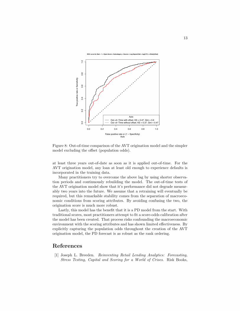
Comparing these two models via an out-of-time test is the ultimate goalof this paper. By including the expected future population odds, the AVTorigination model should out-perform the simpler model without the offset.This is in fact what we observe, Figure 8, to within the granularity of the data.

4 Conclusions

The analysis shown here demonstrates that we can build loan-level models thatare at least as good as conventional scores for rank-ordering, but can also beapplied to forecasting and stress testing. By including the retrending adjust-ment, we guarantee that the model produced will be stationary when extrapo-lated forward or backward, meaning that is can also be used reliably to predictthrough-the-cycle PD estimates simply by providing an average environmentalfunction or macroeconomic scenario.

The AVT origination model created here also has the advantage of beingable to incorporate performance data from the most recent vintages. A stan-dard approach of taking loans originated three years ago and monitoring theirperformance over the next two years to create a score leaves a model that is

13

0.0 0.2 0.4 0.6 0.8 1.0

0.0

0.2

0.4

0.6

0.8

1.0

False positive rate or (1 − Specificity)

Tru

e po

sitiv

e ra

te o

r Sen

sitiv

ity

ROC curve for Bad ~ 1 + Open.Score + Subcategory + Source + Log.Deposit.Bal + log(LTV) + offset(offset)

Auto

AutoOut−of−Time with offset. KS = 0.47. Gini = 0.6Out−of−Time without offset. KS = 0.37. Gini = 0.47

Figure 8: Out-of-time comparison of the AVT origination model and the simplermodel excluding the offset (population odds).

at least three years out-of-date as soon as it is applied out-of-time. For theAVT origination model, any loan at least old enough to experience defaults isincorporated in the training data.

Many practitioners try to overcome the above lag by using shorter observa-tion periods and continuously rebuilding the model. The out-of-time tests ofthe AVT origination model show that it’s performance did not degrade measur-ably two years into the future. We assume that a retraining will eventually berequired, but this remarkable stability comes from the separation of macroeco-nomic conditions from scoring attributes. By avoiding confusing the two, theorigination score is much more robust.

Lastly, this model has the benefit that it is a PD model from the start. Withtraditional scores, most practitioners attempt to fit a score-odds calibration afterthe model has been created. That process risks confounding the macroeconomicenvironment with the scoring attributes and has shown limited effectiveness. Byexplicitly capturing the population odds throughout the creation of the AVTorigination model, the PD forecast is as robust as the rank ordering.

References

[1] Joseph L. Breeden. Reinventing Retail Lending Analytics: Forecasting,Stress Testing, Capital and Scoring for a World of Crises. Risk Books,

14

London, 2010.

[2] Joseph L. Breeden and Lyn C. Thomas. The relationship between defaultand economic cycle for retail portfolios across countries: identifying thedrivers of economic downturn. Journal of Risk Model Validation, 2(3):11 –44, 2008.

[3] Joseph L. Breeden and Lyn C. Thomas. Solutions to specification errors instress testing models. to be published, Journal of the Operational ResearchSociety, 2013.

[4] D. R. Cox and D. O. Oakes. Analysis of Survival Data. Chapman and Hall,London, 1984.

[5] J. Crook and T. Bellotti. Asset correlations for credit card defaults. AppliedFinancial Economics, 22:87–95, 2012.

[6] Bradley Efron. The two-way proportional hazards model. Journal of theRoyal Statistical Society B, 64:899 – 909, 2002.

[7] Norval D. Glenn. Cohort Analysis, 2nd Edition. Sage, London, 2005.

[8] David W. Hosmer, Jr. and Stanley Lemeshow. Applied Survival Analysis:Regression Modeling of Time to Event Data. Wiley Series in Probabilityand Statistics, New York, 1999.

[9] George Judge, William E. Griffiths, R. Carter Hill, Helmut Ltkepohl, andTsoung-Chao Lee. The Theory and Practice of Econometrics. Wiley Publ.,1985.

[10] W.M. Mason and S. Fienberg. Cohort Analysis in Social Research: Beyondthe Identification Problem. Springer, 1985.

[11] Terry M. Therneau and Patricia M. Grambsch. Modeling Survival Data:Extending the Cox Model. Springer-Verlag, New York, 2000.

[12] Lyn C. Thomas. Consumer Credit Models: Pricing, Profit and Portfolios.Oxford University Press, 2009.