Embed Size (px)
Citation preview
Incorporation of dynamic balance
in data assimilation and application to coastal ocean
Zhijin Li and Kayo Ide
SAMSI, Oct. 5, 2005,

First Numerical Weather Predictionby Richardson: 1922
Richardson’s raw data Filtered data (Lynch,2000)
Richardson’s forecast might well have been realistic with the filtered data
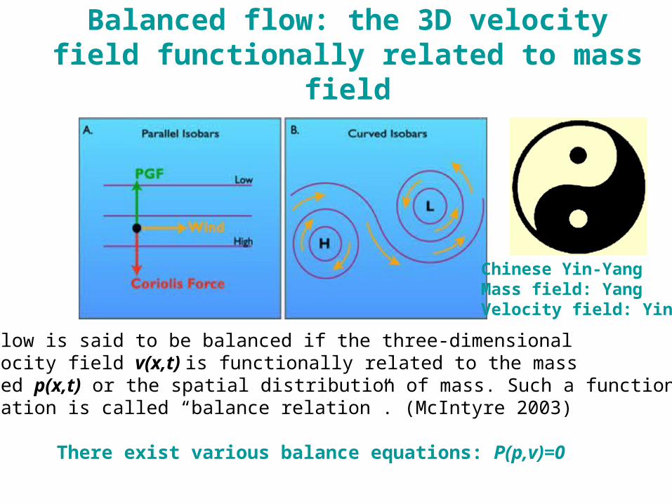
Balanced flow: the 3D velocity field functionally related to mass field
Chinese Yin-YangMass field: YangVelocity field: Yin
A flow is said to be balanced if the three-dimensionalvelocity field v(x,t) is functionally related to the massfiled p(x,t) or the spatial distribution of mass. Such a functionalrelation is called “balance relation”. (McIntyre 2003)
There exist various balance equations: P(p,v)=0
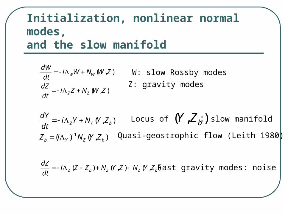
Initialization, nonlinear normal modes, and the slow manifold
),(
),(
ZWNZidt
dZ
ZWNWidt
dW
ZZ
WW
),()(
),(
1bZYb
bYZ
ZYNiZ
ZYNYidt
dY
W: slow Rossby modes
Z: gravity modes
),(),()( bZZbZ ZYNZYNZZidt
dZ
),( bZYLocus of : slow manifold
Fast gravity modes: noise
Quasi-geostrophic flow (Leith 1980)

Slow manifold and data assimilationSlow manifold and data assimilation
S
Y
Z
D
A
L
N O
Schematic slow manifold diagram for a comprehensive model (after Leith 1980; Daley 1980)
Z: fast manifoldY: Rossby manifoldS: slow manifoldD: data manifold => estimate manifold
A: optimal estimateL: linear normal mode initializationN: non-linear normal mode initializationO: optimal estimate with dynamic balance
Data assimilation is suggested to seek O, rather than A.

Why the optimal estimate not on the slow manifold
The true atmospheric and oceanic state weak components of fast gravity modes. Observation observational errors and poor distribution in space and time. A primitive equation model permission of fast gravity modes. Unbalanced error covariance inaccuracy and invalid linearization

A strategy: control variable transform
p
vx
p
vvx u
uup
),(),(
),(),(
),()()()()( 11
ppCvpC
pvCvvCB
yHxRyHxxxBxxxJ oTofTf
),( vpC
),(),(
),(),(
),()()()()( 11
ppCvpC
pvCvvCB
yHxRyHxxxBxxxJ
u
uuuu
oTofuuu
Tfuuu
p
vx v: velocity field; p: mass field
0),( pvpP
Problem: The balance relation works through It may be violatedbecause of inaccurate B, and it is always violated since P is nonlinear.
The balance relation. uv is the unbalanced velocity.

An example for the control
Variable transform: NCEP 3DVAR
Tsfc
f
Wp
QT
Z
DD
)ln(
“The balanced components of the mass and momentum fields have been combined into a single variable. This allows the balance between the mass and momentum fields to be implicitly included.” (Parrish and Derber 1992)
Z is the linear balance operator. The DA control variables: ς, D and f

A refinement:Incremental control variables
p
vx
p
vx
pp
vvvx u
fup
f
)()()( 11 oTopv
T yHxRyHxxBxxJv
v: velocity field; p: mass field
Cost function
Control variables
0),( pvpP Incremental balance relation

Weak geostrophic and hydrostatic balance in a 3DVAR system for coastal ocean: ROMS-DAS
aaTSuv xxx
TSGuv xx
aTS xxx
TSS xx
Geostrophic balance
Vertical integral of the hydrostatic equation
TSfTS
aaTSfuv
aTSf
TS
uv
xx
xxx
xxx
x
x
x
S
T
v
u
x
ax Unbalanced streamfunction and velocity potential

Experiment with a single observation:v-component

ROMS-DAS: Configuration forReal time experiments
12-hour forecast
Time
Aug.100Z
Aug.118Z
Aug.112Z
Aug.106Z
Initialcondition
6-hour forecast
Aug.200Z
Xa = xf + xf
Xa
xf
3-day forecast
y: observationx: model
6-hour assimilation cycle
y
y

Integrated Ocean Observing and Prediction Systems

15 Aug
16 Aug
17 Aug
0
AUV Remus ROMS Reanalysis
18 Aug
Distance (km) 23Subsurface salinity minimalDistance (km) 23Subsurface salinity minimal

Conclusions
With the concept of the slow manifold, it is demonstrated that an additional dynamic constraint is needed to keep the analysis in dynamic balance.
A strategy is suggested that the unbalanced components should be used as control variables to incorporate dynamic balance implicitly in DA.
ROMS-DAS, a 3DVAR system for coastal oceans, has been developed using the strategy. Among the DA control variables are then non-dynamic SSH, adjusted ageostrophic streamfunction and velocity potential.