Incremental Analysis for Probabilistic Programs · Incremental Analysis for Probabilistic Programs Jieyuan Zhang 1, Yulei Sui , and Jingling Xue;2 1 School of Computer Science and

Incremental Analysis for Probabilistic Programs

Jieyuan Zhang1, Yulei Sui1, and Jingling Xue1,2

1 School of Computer Science and Engineering, UNSW Sydney, Australia2 Advanced Innovation Center for Imaging Technology, CNU, China

jieyuan,ysui,[email protected]

Abstract. This paper presents Icpp, a new data-flow-based InCrementalanalysis for Probabilistic Programs, to infer their posterior probabilitydistributions in response to small yet frequent changes to probabilisticknowledge, i.e., prior probability distributions and observations. Unlikeincremental analyses for usual programs, which emphasize code changes,such as statement additions and deletions, Icpp focuses on changes madeto probabilistic knowledge, the key feature in probabilistic programming.The novelty of Icpp lies in capturing the correlation between prior andposterior probability distributions by reasoning about the probabilisticdependence of each data-flow fact, so that any posterior probability af-fected by newly changed probabilistic knowledge can be incrementallyupdated in a sparse manner without recomputing it from scratch, therebyallowing the previously computed results to be reused. We have evaluatedIcpp with a set of probabilistic programs. Our results show that Icppis an order of magnitude faster than the state-of-the-art data-flow-basedinference in analyzing probabilistic programs under small yet frequentchanges to probabilistic knowledge, with an average analysis overhead ofaround 0.1 seconds in response to a single change.

1 Introduction

Uncertainty is a common feature in many modern software systems, especiallystatistical applications (e.g., climate change prediction, spam email filtering andranking the skills of game players). Probabilistic programming provides a power-ful approach to quantifying and characterizing the effects of these uncertainties.A Probabilistic Programming Language (PPL) usually extends an imperativelanguage (e.g., C and Java) by adding two types of language constructs, i.e.,probabilistic assignments for generating random values based on prior probabil-ity distributions and observe statements for conditioning values of variables.

Unlike an imperative program, which is mainly written for the purposes ofbeing executed, a probabilistic program is a specification that specifies implic-itly posterior probability distributions to model uncertainty of the program.Probabilistic inference is the key to reasoning about a probabilistic program byextracting explicit distributions that are implicitly specified in the program.

Generally, there are two approaches to probabilistic inference: (1) dynamicinference, which runs a probabilistic program a finite number of times throughsampling-based Monte Carlo methods [4,7,19,25,28] and then performs inference

2 Jieyuan Zhang, Yulei Sui, and Jingling Xue

to calculate the statistics based on the execution traces, and (2) static inference,which statically computes the probability distributions without repeatedly exe-cuting the program. A typical static method [2] is to abstract a loop-free programas a probabilistic model (e.g., a Bayesian network) and then resorts to existinginference algorithms, e.g., belief propagation [24] and variational inference [35].A recent work, DFI [8], provides more precise inference results than samplingalgorithms and Bayesian modeling methods by applying data-flow analysis toanalyze probabilistic programs with and without loops.

Unlike the case for imperative programs, applying data-flow analysis to infinite-state probabilistic programs is generally more expensive. Data-flow facts of prob-abilistic programs are probability distributions, including the values of programvariables and their corresponding probabilities. Given a probabilistic program,the number of its data-flow facts depends not only on its size parameters but alsothe prior distributions at its probabilistic assignments and the conditions at itsobserve statements. As a common practice in probabilistic programming, prob-abilistic knowledge, which is represented by prior probability distributions andobservations, is often updated under different scenarios or settings [3,6,37]. Toachieve precise modeling, probabilistic assignments and observe statements areoften changed in order to obtain various posterior probability distributions whenwriting a probabilistic program [36]. However, such small yet frequent changesaffect the performance of static inference as the previous inference results becomeinvalid once the program has been modified. Repeatedly reanalyzing a proba-bilistic program that undergoes small changes makes static inference costly.

Incremental analysis aims to efficiently update existing analysis results with-out recomputing them from scratch, allowing the previously computed infor-mation to be reused. There are a few existing works that support incrementalanalysis, such as pointer analysis [18,31], IDE/IFDS analysis [1], data race detec-tion [38], symbolic execution [26], and fixed-point analysis for logic programs [14].However, these existing techniques cannot be directly applied to analyze prob-abilistic programs. For probabilistic programs, frequent changes in probabilisticknowledge pose a new challenge to incremental analysis. It is still an open ques-tion as to whether we can replicate the success of previous incremental analysisfor usual programs in analyzing probabilistic programs.

In this paper, we present Icpp, a new InCremental analysis for analyzingProbabilistic Programs, to infer its posterior probability distributions in re-sponse to small yet frequent changes to probabilistic knowledge, i.e., prior prob-ability distributions and observations. Unlike previous incremental analyses forusual programs, which emphasize code changes, such as statement additions anddeletions, Icpp focuses on changes made to probabilistic knowledge, which is thekey feature in probabilistic programming.

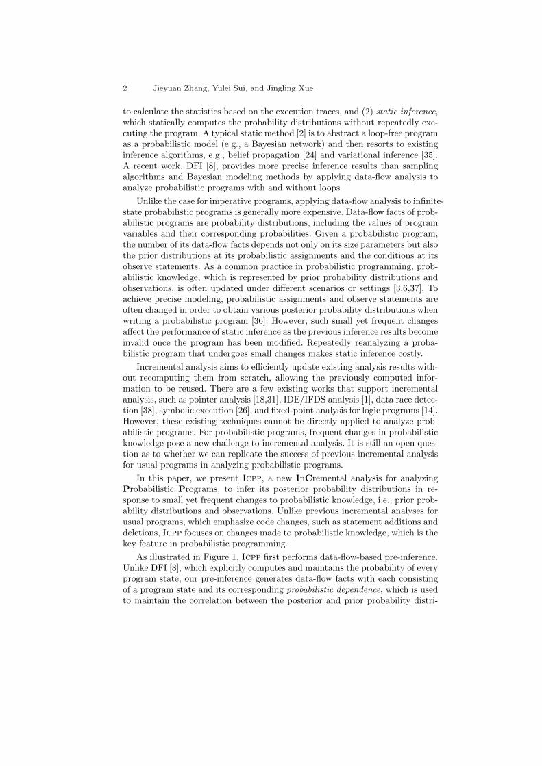
As illustrated in Figure 1, Icpp first performs data-flow-based pre-inference.Unlike DFI [8], which explicitly computes and maintains the probability of everyprogram state, our pre-inference generates data-flow facts with each consistingof a program state and its corresponding probabilistic dependence, which is usedto maintain the correlation between the posterior and prior probability distri-

Incremental Analysis for Probabilistic Programs 3

Retrieve

updateData-flow facts

<program state, probabilistic

dependence>

Pre-InferenceProbabilistic Program

IncrementalInference

PosteriorProbability Distribution

Changes to Probabilistic Knowledge

Once onlyQuery

Output

Fig. 1. Workflow of Icpp.

butions at probabilistic assignments. This probabilistic dependence is later re-trieved to facilitate incremental inference once a change is made to a probabilisticassignment or an observe statement. Based on the dependence information, thedata-flow facts are updated incrementally and propagated sparsely along thecontrol flow to adapt to program changes, making Icpp an instantaneous in-cremental analysis for users to query posterior probability distributions, whileachieving the same precision achieved when the program is re-analyzed entirely.

In summary, the contributions of this paper are as follows:

– We present Icpp, a new InCremental analysis for Probabilistic Programs,in response to small yet frequent changes to probabilistic knowledge.

– We propose a new probabilistic dependence analysis to analyze the twodistinct language constructs in probabilistic programs, probabilistic assign-ments and observe statements.

– We evaluate Icpp using a set of probabilistic programs from R2 [25] andDFI [8]. Our results show that Icpp is an order of magnitude faster thanthe state-of-the-art data-flow-based inference [8] in analyzing these programsunder small yet frequent changes to probabilistic knowledge, with an averageanalysis overhead of around 0.1 seconds in response to a single change.

2 Background

In this section, we describe the preliminaries for our analysis, by focusing on therepresentation and inference of a probabilistic program.

2.1 Probabilistic Programs

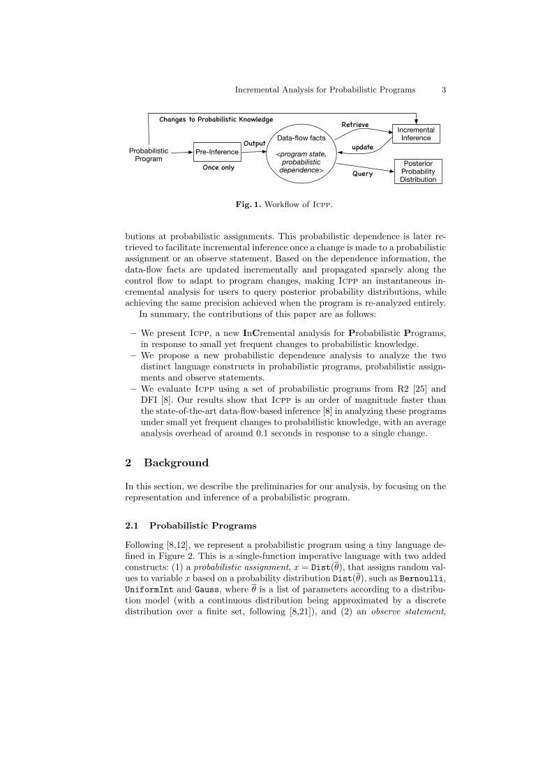
Following [8,12], we represent a probabilistic program using a tiny language de-fined in Figure 2. This is a single-function imperative language with two addedconstructs: (1) a probabilistic assignment, x = Dist(θ), that assigns random val-ues to variable x based on a probability distribution Dist(θ), such as Bernoulli,UniformInt and Gauss, where θ is a list of parameters according to a distribu-tion model (with a continuous distribution being approximated by a discretedistribution over a finite set, following [8,21]), and (2) an observe statement,


x, y, a, b ∈ Vars program variablesθ ∈ R real numbersDist ∈ UniformInt, Bernoulli, Gauss, ... distributionsuop ::= ++,−−, ! unary operationsbop ::= +,−,×, /,&&, ||,==, 6=, <,>,≤,≥ binary operations

E ::= expressions| x variable| c constant| E1 bop E2 binary operation| uop E unary operation

` ::= labeled statements| x = E deterministic assignment| `1; `2 sequential composition| if E then `1 else `2 conditional composition| while E do ` loop| skip skip

| x = Dist(θ) probabilistic assignment| observe(E) observe

Prog ::= ` program

Fig. 2. Syntax of a probabilistic program.

observe(E), that conditions the expression E to be true. The effect of the ob-serve statement is to block all program executions violating condition E .

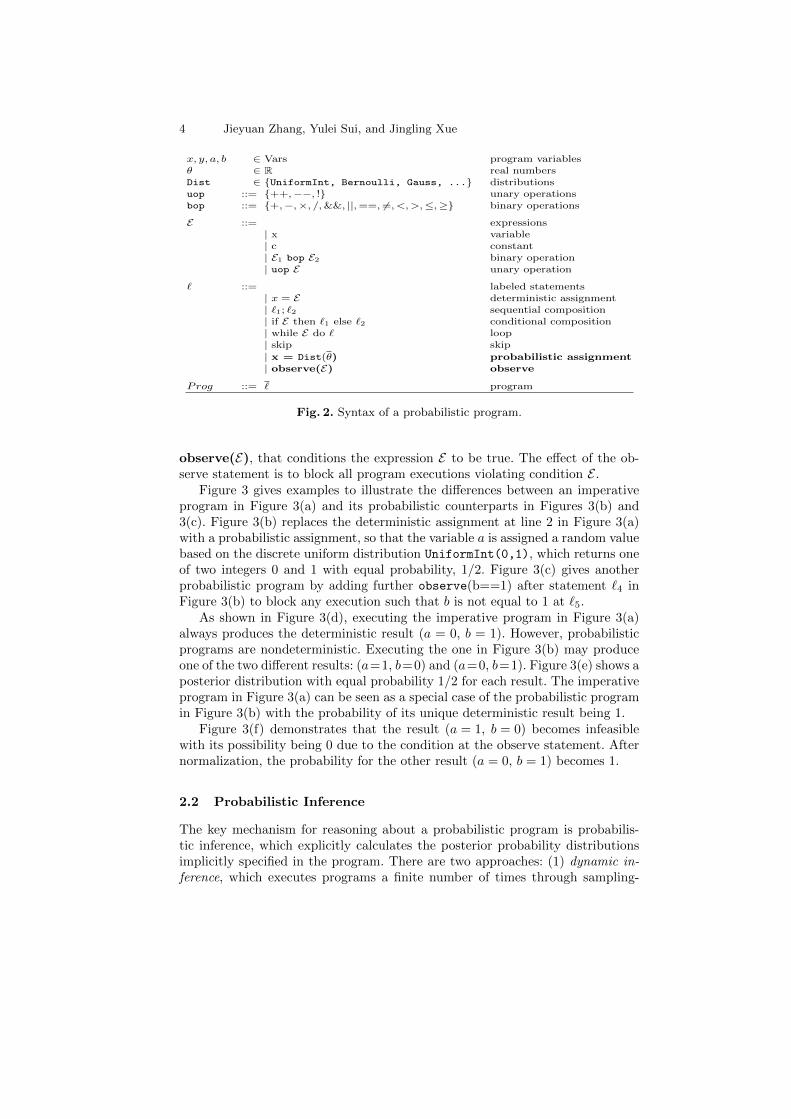
Figure 3 gives examples to illustrate the differences between an imperativeprogram in Figure 3(a) and its probabilistic counterparts in Figures 3(b) and3(c). Figure 3(b) replaces the deterministic assignment at line 2 in Figure 3(a)with a probabilistic assignment, so that the variable a is assigned a random valuebased on the discrete uniform distribution UniformInt(0,1), which returns oneof two integers 0 and 1 with equal probability, 1/2. Figure 3(c) gives anotherprobabilistic program by adding further observe(b==1) after statement `4 inFigure 3(b) to block any execution such that b is not equal to 1 at `5.

As shown in Figure 3(d), executing the imperative program in Figure 3(a)always produces the deterministic result (a = 0, b = 1). However, probabilisticprograms are nondeterministic. Executing the one in Figure 3(b) may produceone of the two different results: (a=1, b=0) and (a=0, b=1). Figure 3(e) shows aposterior distribution with equal probability 1/2 for each result. The imperativeprogram in Figure 3(a) can be seen as a special case of the probabilistic programin Figure 3(b) with the probability of its unique deterministic result being 1.

Figure 3(f) demonstrates that the result (a = 1, b = 0) becomes infeasiblewith its possibility being 0 due to the condition at the observe statement. Afternormalization, the probability for the other result (a = 0, b = 1) becomes 1.

2.2 Probabilistic Inference

The key mechanism for reasoning about a probabilistic program is probabilis-tic inference, which explicitly calculates the posterior probability distributionsimplicitly specified in the program. There are two approaches: (1) dynamic in-ference, which executes programs a finite number of times through sampling-


ℓ1: bool a=1;ℓ2: int b=1;ℓ3: if (b>0)ℓ4: a=!a;

ℓ1: bool a=1;ℓ2: int b=uniformInt(0,1);ℓ3: if (b>0)ℓ4: a=!a;ℓ5: observe(b==1);

(a) Imperative program (b) Probabilistic assignment (added) (c) Observe statement (added further)

1/2(a=1, b=0) 1/2(a=0, b=1)(a=0, b=1)

What are the values of a and b at the end of every program?

(d) Deterministic result for program (a)

(e) Posterior probability distribution for program (b)

(f) Posterior probability distribution for program (c)

(a=1, b=0)(a=0, b=1) 1

0

ℓ1: bool a=1;ℓ2: int b=uniformInt(0,1);ℓ3: if (b>0)ℓ4: a=!a;

Fig. 3. Imperative vs. probabilistic programs.

based methods [19], such as importance sampling [11], Gibbs sampling [28] andMetropolis-Hastings sampling [7], and (2) static inference, which computes theprobability distributions statically without running the program.

A recent data-flow-based inference, DFI [8], applies the data-flow theory forprobabilistic inference by treating probability distributions as data-flow facts.DFI is path-sensitive by analyzing control-flow branch conditions. The resultinginference provides better precision than many existing methods, e.g., Expecta-tion Propagation [22], message passing algorithm [16] and MCMC sampling [13].

In DFI, the static inference is formulated as a forward data-flow problem(D,u, F ). Here, D represents all data-flow facts with each 〈σ, ρ〉 ∈ D consistingof a program state σ (a set of values) and its corresponding probability ρ when σholds. u is the meet operator. F : D → D represents the set of transfer functionswith f` being associated with node (statement) at ` in the CFG of the program.

A path-sensitive analysis computes the data-flow facts (probability distri-butions) by considering every executable path. We write π to denote a path[`1, `2 . . . `n] consisting a sequence of n statements in a CFG. The transfer func-tion for π is fπ ∈ F , which is the composition of transfer functions of the firstn − 1 statements on π, i.e., fπ = f`1 f`2 . . . f`n−1

. Note that we speak of thepath π by excluding the last statement at `n. Finally, the set of data-flow facts,D`n, that reach the beginning of a statement `n is computed as follows:

D`n = ⊔

π∈paths(`n)

fπ(>) (1)

where paths(`n) denotes the set of paths from the program entry to statement`n and > ∈ D is the standard top element in the lattice used.

When analyzing a statement ` in DFI [8], its transfer function f`, which isdefined based on the standard Gen/Kill sets, is distributive, so that f`(d1) ∪f`(d2) = f`(d1 ∪ d2) holds, where d1, d2 ∈ D. Therefore, the meet operator u isthe set union (∪), causing the data-flow facts at a joint point to be merged, inorder to reduce the number of facts propagated without affecting the precision of


else

Dℓ5

Dℓ4

Dℓ3

Dℓ2

ℓ1: a=1

ℓ2: b=UniformInt(0,1)

ℓ3: if (b>0)

ℓ4: a=!a

ℓ5: observe(a==1)

ℓ6: end

<(a=1), 1>

<(a=1, b=0), 1/2><(a=1, b=1), 1/2>

<(a=1, b=1), 1/2>

∅

if

Dℓ6

<(a=1, b=0), 1/2><(a=0, b=1), 1/2>

Dℓ1

[ℓ1, ℓ2, ℓ3, ℓ4];[ℓ1, ℓ2, ℓ3];

[ℓ1];

[ℓ1, ℓ2];

[ℓ1, ℓ2, ℓ3];

[ℓ1, ℓ2, ℓ3, ℓ4, ℓ5];[ℓ1, ℓ2, ℓ3, ℓ5]; <(a=0, b=1), 0 >

<(a=1, b=0), 1/2>

path along if branch: [ℓ1, ℓ2, ℓ3, ℓ4, ℓ5]

path along else branch: [ℓ1, ℓ2, ℓ3, ℓ5];

Data-flow facts <!, ">

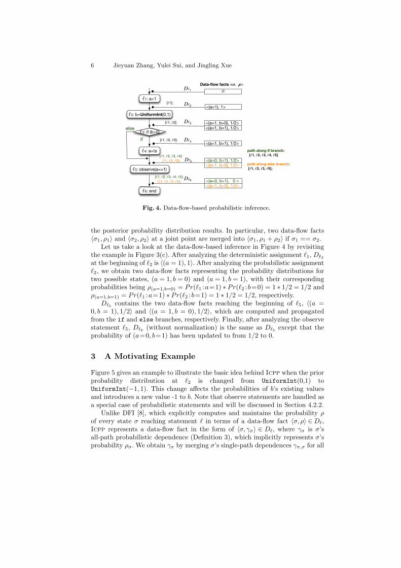
Fig. 4. Data-flow-based probabilistic inference.

the posterior probability distribution results. In particular, two data-flow facts〈σ1, ρ1〉 and 〈σ2, ρ2〉 at a joint point are merged into 〈σ1, ρ1 + ρ2〉 if σ1 == σ2.

Let us take a look at the data-flow-based inference in Figure 4 by revisitingthe example in Figure 3(c). After analyzing the deterministic assignment `1, D`2

at the beginning of `2 is 〈(a = 1), 1〉. After analyzing the probabilistic assignment`2, we obtain two data-flow facts representing the probability distributions fortwo possible states, (a = 1, b = 0) and (a = 1, b = 1), with their correspondingprobabilities being ρ(a=1,b=0) = Pr(`1 :a=1) ∗ Pr(`2 :b=0) = 1 ∗ 1/2 = 1/2 andρ(a=1,b=1) = Pr(`1 :a=1) ∗ Pr(`2 :b=1) = 1 ∗ 1/2 = 1/2, respectively.

D`5 contains the two data-flow facts reaching the beginning of `5, 〈(a =0, b = 1), 1/2〉 and 〈(a = 1, b = 0), 1/2〉, which are computed and propagatedfrom the if and else branches, respectively. Finally, after analyzing the observestatement `5, D`6 (without normalization) is the same as D`5 except that theprobability of (a=0, b=1) has been updated to from 1/2 to 0.

3 A Motivating Example

Figure 5 gives an example to illustrate the basic idea behind Icpp when the priorprobability distribution at `2 is changed from UniformInt(0,1) toUniformInt(−1, 1). This change affects the probabilities of b’s existing valuesand introduces a new value -1 to b. Note that observe statements are handled asa special case of probabilistic statements and will be discussed in Section 4.2.2.

Unlike DFI [8], which explicitly computes and maintains the probability ρof every state σ reaching statement ` in terms of a data-flow fact 〈σ, ρ〉 ∈D`,Icpp represents a data-flow fact in the form of 〈σ, γσ〉 ∈ D`, where γσ is σ’sall-path probabilistic dependence (Definition 3), which implicitly represents σ’sprobability ρσ. We obtain γσ by merging σ’s single-path dependences γπ,σ for all


the paths π reaching ` (Definition 2), where γπ,σ collects the probability seedsgenerated from the relevant probabilistic assignments on π (Definition 1). Whenbuilding a particular single-path dependence γπ,σ, only one single seed is selectedfor a probabilistic assignment every time when it is analyzed. Therefore, a seedmay appear multiple times in γπ,σ when π contains a loop, which is handled byapproximating a KL-divergence [22] between two consecutive loop iterations.

Definition 1 (Probability Seed). For a probabilistic assignment ` : x =Dist(θ), we define a probability seed at ` as s = 〈` :x = a〉, where a is one of allthe possible values returned by the prior distribution Dist(θ). One probabilisticassignment ` may induce multiple seeds s ∈ Seeds(`) from the distribution.

Definition 2 (Single-Path Probabilistic Dependence). For a data-flowfact 〈σ, γπ,σ〉∈fπ(>) associated with path π = [`1, . . . , `n], its single-path proba-bilistic dependence is γπ,σ = [s1, . . . , sm], which consists of a sequence of probabil-ity seeds (Definition 1) based on all the probabilistic assignments on π (m < n).The probability of σ for π is ρπ,σ = Pr(γπ,σ) = Pr(s1) ∗ Pr(s2) ∗ · · · ∗ Pr(sm).

Definition 3 (All-Path Probabilistic Dependence). For a data-flow fact〈σ, γσ〉 ∈ D` at the beginning of `, its all-path probabilistic dependence γσ =γπ,σ | π ∈ paths(`) consists of the dependence information for every singlepath π reaching `, with σ’s probability being ρσ = Pr(γσ) = Σπ∈paths(`) ρπ,σ.

Let us look at the example in Figure 5 to illustrate how Icpp incrementallycomputes the posterior probability distributions at `6 once the prior probabil-ity distribution at a probabilistic assignment is changed. Pre-inference is firstperformed to generate the probabilistic dependences for all the data-flow factsduring the on-the-fly data-flow analysis. Based on the dependence information,sparse incremental update is performed to recalculate the posterior probabilitydistributions of the existing data-flow facts at `6 affected by the change made.Finally, we propagate the new data-flow facts introduced by the change acrossthe entire program in a sparse manner via sparse incremental propagation.

Pre-inference. For the program given in Figure 5(a), the data-flow facts ob-tained by pre-inference are listed in Figure 5(b).

To start with, the probabilistic assignment `1 based on the Bernoulli distri-bution assigns a random value 0 or 1 to variable a with each value’s probabilitybeing 1/2. As shown, D`2 therefore contains the two data-flow facts, where theprobabilistic dependence of each state is its corresponding probability seed gen-erated from `1 (e.g., (a = 0) is annotated with its seed [`1 :a = 0]).

The probabilistic assignment at `2 gives variable b a random value, 0 or 1,based on a discrete uniform distribution. By combining with the two values ofvariable a, we obtain the four data-flow facts in D`3 to represent the four possiblestates for a and b with the probability of each state being 1/4. The correspondingprobabilistic dependence of each state (e.g., (a = 0, b = 0)) is a sequence ofprobability seeds (e.g., [`1 : a = 0, `2 : b = 0]), which are used to compute itscorresponding probability (e.g., ρ(a=0,b=0) = Pr(`1 :a = 0)∗Pr(`2 :b = 0) = 1/4).


ℓ1: a=Bernoulli(0.5)


ℓ3: if (b>0)

ℓ4: a=!a


1/21/2

<(a=1),[ℓ1: a=1]><(a=0),[ℓ1: a=0]>

1/41/4

1/41/4

<(a=0,b=1),[ℓ1: a=0, ℓ2: b=1]><(a=0,b=0),[ℓ1: a=0, ℓ2: b=0]>

<(a=1,b=0),[ℓ1: a=1, ℓ2: b=0]><(a=1,b=1),[ℓ1: a=1, ℓ2: b=1]>

<(a=0,b=1),[ℓ1: a=0, ℓ2: b=1]>1/41/4

<(a=1,b=1),[ℓ1: a=1, ℓ2: b=1]>

ℓ6: end

...

...unchanged <…>unchanged <…>

1/41/4<(a=1,b=1),[ℓ1: a=0, ℓ2: b=1]>

<(a=0,b=1),[ℓ1: a=1, ℓ2: b=1]>

(b) Pre-inference results of the original program

Sparse Incremental

Update

Data-flow facts <!, "!> #!

Inference results of original program

Dℓ2

Dℓ3

Dℓ4

elseif

Dℓ5

Dℓ6

Dependence Look up

Dℓ1

path along if branch: [ℓ1, ℓ2, ℓ3, ℓ4, ℓ5, ℓ6] path along else branch: [ℓ1, ℓ2, ℓ3 ℓ6];

∅

unchanged <…> 1/12

unchanged <…>

<(a=0,b=-1),(ℓ1: a=0, ℓ2: b=-1)>

1/4

1/6

1/4<(a=1,b=-1),(ℓ1: a=1, ℓ2: b=-1)>

unchanged <…>

unchanged <…>

1/6

1/12

Sparse incrementalpropagation

gene

rate

d ne

w fa

cts

(c) Incremental inference results of the modified program(a) A program and its CFG

<(a=0,b=1),[ℓ1: a=1, ℓ2: b=1, ℓ5: b=1]> 1/8

1/8+

1/4<(a=0,b=0),[ℓ1: a=1, ℓ2: b=1, ℓ5: b=0], [ℓ1: a=0, ℓ2: b=0]>

<(a=1,b=1),[ℓ1: a=0, ℓ2: b=1, ℓ5: b=1]> 1/8

<(a=1,b=0),[ℓ1: a=0, ℓ2: b=1, ℓ5: b=0], [ℓ1: a=1, ℓ2: b=0]>

1/8+

1/4

1/6<(a=1,b=-1),(ℓ1: a=1, ℓ2: b=-1)>1/6<(a=0,b=-1),(ℓ1: a=0, ℓ2: b=-1)>

...

...

...


unchanged <…>unchanged <…>

prob

abilit

y ch

ange

s to

the

exist

ing fa

cts

All-path probabilistic dependence:

Data-flow facts <!, "!> #!

Inference results after changing ℓ2 to b=UniformInt(-1,1)

...


...


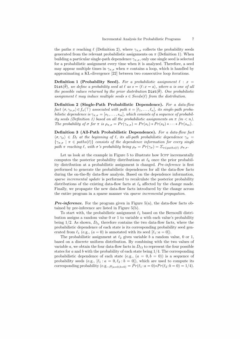
Fig. 5. A motivating example illustrating how Icpp works in response to the changeat `2 from UniformInt(0,1) to UniformInt(−1, 1) (as highlighted in red).

There are two branches at `3 when propagating D`3 forward. Only two data-flow facts whose states satisfy condition b > 0 are propagated to the if branch asillustrated in D`4 while the other two are propagated to the else branch. Afteranalyzing `4, a’s value in each data-flow fact of D`4 is flipped, while b’s valuestays the same. Note that the probabilistic dependence recorded in each data-flow fact remains unchanged, as indicated in D`5 , because `4 is a deterministicstatement, which does not affect any probabilistic dependence in any way.

After analyzing `5, D`6 contains six data-flow facts at the join point before`6 (the end of the program). The four data-flow facts highlighted in green aregenerated after analyzing `5 in the if branch and the two data-flow facts inorange are propagated from the else branch. Let πif = [`1, `2, `3, `4, `5, `6] andπelse = [`1, `2, `3, `6] as shown in Figure 5(b). The data-flow facts whose statesare the same are merged by computing their all-path probabilistic dependence(Definition 3). Therefore, 〈(a = 0, b = 0), γπif ,(a=0,b=0)〉 from the if branch and〈(a = 0, b = 0), γπelse,(a=0,b=0)〉 from the else branch are merged into 〈(a =0, b = 0), γπif ,(a=0,b=0), γπelse,(a=0,b=0)〉, where

γπif ,(a=0,b=0) = [`1 :a = 1, `2 :b = 1, `5 :b = 0]γπelse,(a=0,b=0) = [`1 :a = 0, `2 :b = 0]

(2)


Likewise, the two data-flow facts with the same state (a = 1, b = 0) are alsomerged. Finally, we calculate the joint posterior probability ρσ for each data-flowfact reaching `6 based on its probabilistic dependence as shown in Figure 5(b).

Sparse Incremental Update. Here, our incremental analysis is concernedwith updating the posterior probabilities of the existing data-flow facts in D`6 ,which are affected by the changes made to the prior probability distributions dis-covered by the computed probabilistic dependences. Icpp does not reanalyze theprogram to recompute any of the existing data-flow facts 〈σ, γσ〉 ∈ D`6 . Instead,it just recalculates its posterior probability ρσ. For example, the probabilisticassignment `2, changed from b = UniformInt(0, 1) to b = UniformInt(−1, 1),causes the prior probabilities of the two probability seeds to change from Prold(`2 :b = 0) = Prold(`2 : b = 1) = 1/2 to Prnew(`2 : b = 0) = Prnew(`2 : b = 1) = 1/3.In this motivating example, we are interested in the effects of the change on theposterior probabilities at `6. As shown in Figure 5(b), D`6 contains four data-flowfacts that are computed before the change is made. Therefore, their probabilitiesneed to be updated. Consider first 〈(a = 0, b = 0), γπif ,(a=0,b=0), γπelse,(a=0,b=0)〉,where γπif ,(a=0,b=0) and γπelse,(a=0,b=0) are given in (2). The following equationrecalculates the posterior probability of its corresponding state (a = 0, b = 0),whose probabilistic dependence contains the two probability seeds, `2 : b = 0and `2 : b = 1:

ρnew(a=0,b=0) =Prold(γπif ,(a=0,b=0) ∗ Prnew(`2 :b = 1)

Prold(`2 :b = 1)

+Prold(γπelse,(a=0,b=0) ∗ Prnew(`2 :b = 0)

Prold(`2 :b = 0)

=1/8 ∗ 1/3

1/2+

1/4 ∗ 1/3

1/2= 1/4

Likewise, the probabilities of the other three data-flow facts in D`6 are updatedas ρnew(a=1,b=0) = 1/4, ρnew(a=1,b=1) = 1/12 and ρnew(a=0,b=1) = 1/12. These updated

posterior probabilities are reflected in the bottom of Figure 5(c).Updating existing data-flow facts incrementally this way is lightweight. As

we are interested in the effects of a change on `6 in our motivating example, theposterior probabilities for the data-flow facts in D`6 are recalculated directly. Allthe other data-flow facts from D`1 to D`5 remain untouched, without requiringany expensive data-flow analysis that computes and propagates data-flow facts(probabilistic dependences) along the program’s control-flow.

Sparse Incremental Propagation. The change made to the prior probabilitydistribution at `2 also introduces a new probability seed [`2 : b = −1] with itsprobability Pr(`2 :b = −1) = 1/3, as illustrated in Figure 5(c). During the sparseincremental propagation, the two new data-flow facts, 〈(a = 0, b = −1), [`1 :a =0, `2 : b = −1]〉 and 〈(a = 1, b = −1), [`1 : a = 1, `2 : b = −1]〉, are generatedand appended to D`3 . In general, the new data-flow facts generated this way are


propagated sparsely along the control flow in the program, without causing theexisting data-flow facts to be modified. Finally, we obtain the updated posteriorjoint distributions at `6 by combining the results of both existing and new data-flow facts incrementally computed for `6, as shown in Figure 5(c).

4 ICPP: Incremental Analysis for Probabilistic Programs

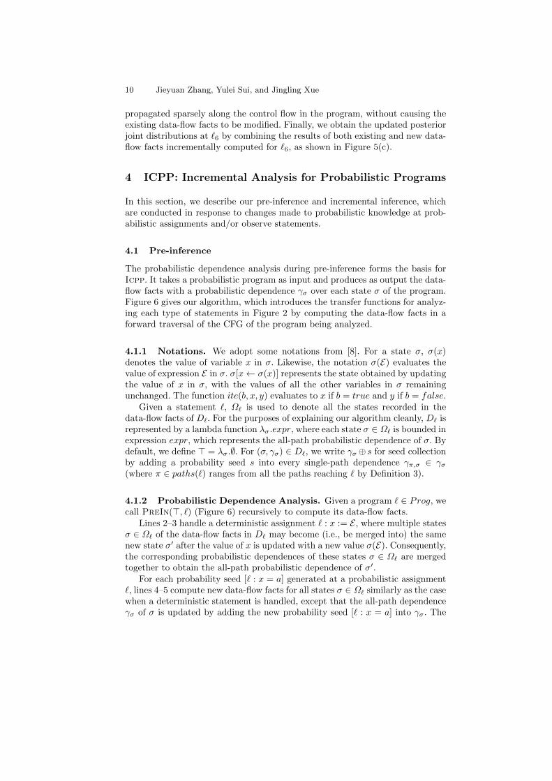
In this section, we describe our pre-inference and incremental inference, whichare conducted in response to changes made to probabilistic knowledge at prob-abilistic assignments and/or observe statements.

4.1 Pre-inference

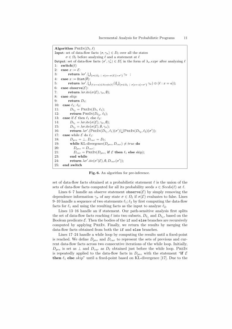
The probabilistic dependence analysis during pre-inference forms the basis forIcpp. It takes a probabilistic program as input and produces as output the data-flow facts with a probabilistic dependence γσ over each state σ of the program.Figure 6 gives our algorithm, which introduces the transfer functions for analyz-ing each type of statements in Figure 2 by computing the data-flow facts in aforward traversal of the CFG of the program being analyzed.

4.1.1 Notations. We adopt some notations from [8]. For a state σ, σ(x)denotes the value of variable x in σ. Likewise, the notation σ(E) evaluates thevalue of expression E in σ. σ[x← σ(x)] represents the state obtained by updatingthe value of x in σ, with the values of all the other variables in σ remainingunchanged. The function ite(b, x, y) evaluates to x if b = true and y if b = false.

Given a statement `, Ω` is used to denote all the states recorded in thedata-flow facts of D`. For the purposes of explaining our algorithm cleanly, D` isrepresented by a lambda function λσ.expr, where each state σ ∈ Ω` is bounded inexpression expr, which represents the all-path probabilistic dependence of σ. Bydefault, we define > = λσ.∅. For (σ, γσ) ∈ D`, we write γσ⊕ s for seed collectionby adding a probability seed s into every single-path dependence γπ,σ ∈ γσ(where π ∈ paths(`) ranges from all the paths reaching ` by Definition 3).

4.1.2 Probabilistic Dependence Analysis. Given a program ` ∈ Prog, wecall PreIn(>, `) (Figure 6) recursively to compute its data-flow facts.

Lines 2–3 handle a deterministic assignment ` : x := E , where multiple statesσ ∈ Ω` of the data-flow facts in D` may become (i.e., be merged into) the samenew state σ′ after the value of x is updated with a new value σ(E). Consequently,the corresponding probabilistic dependences of these states σ ∈ Ω` are mergedtogether to obtain the all-path probabilistic dependence of σ′.

For each probability seed [` : x = a] generated at a probabilistic assignment`, lines 4–5 compute new data-flow facts for all states σ ∈ Ω` similarly as the casewhen a deterministic statement is handled, except that the all-path dependenceγσ of σ is updated by adding the new probability seed [` : x = a] into γσ. The


Algorithm PreIn(D`, `)Input: set of data-flow facts 〈σ, γσ〉 ∈ D` over all the states

σ ∈ Ω` before analyzing ` and a statement at Òutput: set of data-flow facts 〈σ′, γ′σ〉 ∈ D′` in the form of λσ.expr after analyzing `1: switch(`)2: case x := E :3: return λσ′.

⋃σ∈Ω` | σ[x←σ(E)]=σ′

γσ ;

4: case x := Dist(θ):5: return λσ′.

⋃(`:x=a)∈Seeds(`)((

⋃σ∈Ω` | σ[x←a]=σ′

γσ)⊕ (` : x = a));

6: case observe(E):7: return λσ.ite(σ(E), γσ, ∅);8: case skip:9: return D`;10: case `1; `2:11: D`2 = PreIn(D`, `1);12: return PreIn(D`2 , `2);13: case if E then `1 else `2:14: D`1 = λσ.ite(σ(E), γσ, ∅);15: D`2 = λσ.ite(σ(E), ∅, γσ);16: return λσ′.(PreIn(D`1 , `1)(σ′)

⋃PreIn(D`2 , `2)(σ′));

17: case while E do `1:18: Dpre = ⊥, Dcur = D`;19: while KL-divergence(Dpre, Dcur) 6= true do20: Dpre = Dcur;21: Dcur = PreIn(Dpre, if E then `1 else skip);23: end while24: return λσ′.ite(σ′(E), ∅, Dcur(σ′));25: end switch

Fig. 6. An algorithm for pre-inference.

set of data-flow facts obtained at a probabilistic statement ` is the union of thesets of data-flow facts computed for all its probability seeds s ∈ Seeds(`) at `.

Lines 6–7 handle an observe statement observe(E) by simply removing thedependence information γσ of any state σ ∈ Ω` if σ(E) evaluates to false. Lines9–10 handle a sequence of two statements `1; `2 by first computing the data-flowfacts for `1 and using the resulting facts as the input to analyze `2.

Lines 13–16 handle an if statement. Our path-sensitive analysis first splitsthe set of data-flow facts reaching ` into two subsets, D`1 and D`2 , based on theBoolean predicate E . Then the bodies of the if and else branches are recursivelycomputed by applying PreIn. Finally, we return the results by merging thedata-flow facts obtained from both the if and else branches.

Lines 17–24 handle a while loop by computing the results until a fixed-pointis reached. We define Dpre and Dcur to represent the sets of previous and cur-rent data-flow facts across two consecutive iterations of the while loop. Initially,Dpre is set as ⊥ and Dcur as D` obtained just before the while loop. PreInis repeatedly applied to the data-flow facts in Dpre with the statement “if Ethen `1 else skip” until a fixed-point based on KL-divergence [17]. Due to the


non-determinism of probabilistic programs [8,10,12] (e.g., a probabilistic assign-ment generates a probability seed randomly during each loop iteration), findinga loop iteration under which Dcur = Dpre is potentially nonterminating. Thus,we use KL-divergence to enforce the termination of a while loop. In line 19,KL-divergence(Dcur, Dpre) is true if the following condition holds:

|∑

σ∈Ωcur

ρσ ∗ ln(ρσρ′σ

) | < threshold (3)

where ρσ is the probability of σ ∈ Ωcur calculated based on 〈σ, γσ〉 ∈ Dcur, ρ′σ

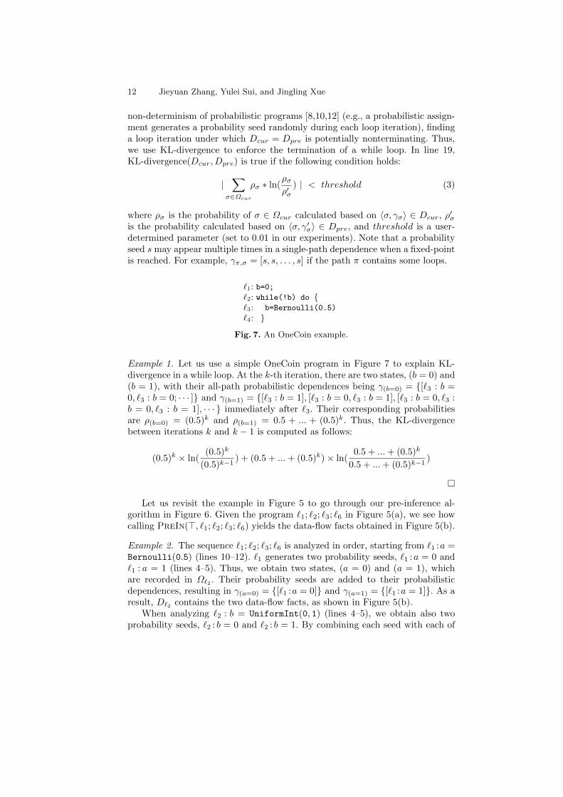
is the probability calculated based on 〈σ, γ′σ〉 ∈ Dpre, and threshold is a user-determined parameter (set to 0.01 in our experiments). Note that a probabilityseed s may appear multiple times in a single-path dependence when a fixed-pointis reached. For example, γπ,σ = [s, s, . . . , s] if the path π contains some loops.

`1: b=0;`2: while(!b) do `3: b=Bernoulli(0.5)

`4:

Fig. 7. An OneCoin example.

Example 1. Let us use a simple OneCoin program in Figure 7 to explain KL-divergence in a while loop. At the k-th iteration, there are two states, (b = 0) and(b = 1), with their all-path probabilistic dependences being γ(b=0) = [`3 : b =0, `3 : b = 0; · · · ] and γ(b=1) = [`3 : b = 1], [`3 : b = 0, `3 : b = 1], [`3 : b = 0, `3 :b = 0, `3 : b = 1], · · · immediately after `3. Their corresponding probabilitiesare ρ(b=0) = (0.5)k and ρ(b=1) = 0.5 + ... + (0.5)k. Thus, the KL-divergencebetween iterations k and k − 1 is computed as follows:

(0.5)k × ln((0.5)k

(0.5)k−1) + (0.5 + ...+ (0.5)k)× ln(

0.5 + ...+ (0.5)k

0.5 + ...+ (0.5)k−1)

Let us revisit the example in Figure 5 to go through our pre-inference al-gorithm in Figure 6. Given the program `1; `2; `3; `6 in Figure 5(a), we see howcalling PreIn(>, `1; `2; `3; `6) yields the data-flow facts obtained in Figure 5(b).

Example 2. The sequence `1; `2; `3; `6 is analyzed in order, starting from `1 :a =Bernoulli(0.5) (lines 10–12). `1 generates two probability seeds, `1 :a = 0 and`1 : a = 1 (lines 4–5). Thus, we obtain two states, (a = 0) and (a = 1), whichare recorded in Ω`2 . Their probability seeds are added to their probabilisticdependences, resulting in γ(a=0) = [`1 :a = 0] and γ(a=1) = [`1 :a = 1]. As aresult, D`2 contains the two data-flow facts, as shown in Figure 5(b).

When analyzing `2 : b = UniformInt(0, 1) (lines 4–5), we obtain also twoprobability seeds, `2 : b = 0 and `2 : b = 1. By combining each seed with each of


the two states in Ω`2 = (a = 0), (a = 1), we obtain the four states in D`3 , asshown in Figure 5(b), with the probabilistic dependence γσ of each state σ ∈ Ω`3containing an additional probability seed of either `2 : b = 0 or `2 : b = 1. As aresult, D`3 contains the four data-flow facts, as shown in Figure 5(b).

When analyzing `3 : if (b > 0) then `4; `5 else skip (lines 13–16), we splitD`3 into D`4;`5 and Dskip according to the condition b > 0, where D`4;`5 ispropagated into the if branch and and Dskip into the else branch. Then wecontinue to apply PreIn to compute the data-flow facts for `4; `5 (lines 10–12)and skip (lines 8–9). Finally, we merge the data-flow facts flowing out of the twobranches at the beginning of `6 to obtain D`6 (line 16).

4.2 Incremental Inference

Based on the computed probabilistic dependence information, our incrementalanalysis handles two type of changes made to a probabilistic program, i.e, priordistribution changes at a probabilistic assignment (Section 4.2.1) and conditionchanges at an observe statement (Section 4.2.2). Icpp aims to recalculate theposterior probability ρσ for each data-flow fact 〈σ, γσ〉 ∈ Dènd at ènd (the end ofa program) according to the computed probabilistic dependence γσ, in responseto the changes made to probabilistic knowledge in the program.

Without loss of generality, we restrict ourselves to a change made to one singlestatement at a time. Our incremental inference generalizes straightforwardly tothe changes made simultaneously to multiple statements.

4.2.1 Handling Changes Made at Probabilistic Assignments. For aprobabilistic assignment x = Dist(θ), Icpp focuses on a change made to theprior distribution Dist(θ), which is defined over a measurable sample spacewith a probability measure. Thus, a change can be a modification of the samplespace or the probability measure. For example, if x=Bernoulli(0.5) is modifiedto x = Bernoulli(0.6), the sample space, 0, 1, remains the same, but theprobability measure is adjusted, with the probability of x=1 changed from 0.5and 0.6. However, modifying x= UniformInt(0, 1) into x= UniformInt(−1, 1)will change both its sample space and probability measure. Similarly, modifyinga distribution model from Dist to Dist′ also affects both.

Modifying a probability measure changes the posterior probabilities of exist-ing data-flow facts computed by pre-inference. Modifying a sample space gener-ates new probability seeds, and consequently, introduces new data-flow facts.

For a change made at a probabilistic assignment, the algorithm in Figure 8updates the posterior probabilities of the existing data-flow facts affected viaIncUpdate and propagates the newly introduced data-flow facts via IncProp.

Sparse Incremental Update. According to our algorithm in Figure 8, Scom =Seeds(òld) ∩ Seeds(`new) is the set of probability seeds that exist in both theoriginal and modified programs. Dènd is the set of data-flow facts that reach èndcomputed before the change. IncUpdate(Dènd , S

com) can instantly recalculate


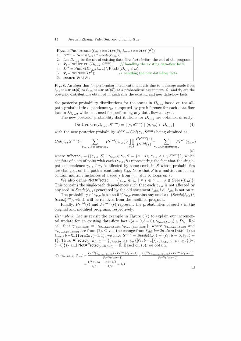
HandleProbAssign(òld : x=Dist(θ), `new : x=Dist′(θ′))

1: Scom = Seeds(òld) ∩ Seeds(`new);2: Let Dènd be the set of existing data-flow facts before the end of the program;3: Ψ1=IncUpdate(Dènd , S

com); // handling the existing data-flow facts4: D∆ = PreIn(Dòld , `new) \ PreIn(Dòld , òld);5: Ψ2=IncProp(D∆); // handling the new data-flow facts6: return Ψ1 ∪ Ψ2;

Fig. 8. An algorithm for performing incremental analysis due to a change made fromòld :x=Dist(θ) to `new :x=Dist′(θ

′) at a probabilistic assignment. Ψ1 and Ψ2 are the

posterior distributions obtained in analyzing the existing and new data-flow facts.

the posterior probability distributions for the states in Dènd based on the all-path probabilistic dependence γσ computed by pre-inference for each data-flowfact in Dènd , without a need for performing any data-flow analysis.

The new posterior probability distributions for Dènd are obtained directly:

IncUpdate(Dènd , Scom) = 〈σ, ρnewσ 〉 | 〈σ, γσ〉 ∈ Dènd (4)

with the new posterior probability ρnewσ = Cal(γσ, Scom) being obtained as:

Cal(γσ, Scom)=

∑(γπ,σ,S)∈Affectedσ

Prold(γπ,σ)×∏s∈S

Prnew(s)

Prold(s)+

∑γπ,σ∈NotAffectedσ

Prold(γπ,σ)

(5)where Affectedσ = (γπ,σ, S) | γπ,σ ∈ γσ, S = s | s ∈ γπ,σ ∧ s ∈ Scom, whichconsists of a set of pairs with each (γπ,σ, S) representing the fact that the single-path dependence γπ,σ ∈ γσ is affected by some seeds in S whose probabilitiesare changed, on the path π containing òld. Note that S is a multiset as it maycontain multiple instances of a seed s from γπ,σ due to loops on π.

We also define NotAffectedσ = γπ,σ ∈ γσ | ∀ s ∈ γπ,σ : s 6∈ Seeds(òld).This contains the single-path dependences such that each γπ,σ is not affected byany seed in Seeds(òld) generated by the old statement òld, i.e., òld is not on π.

The probability of γπ,σ is set to 0 if γπ,σ contains any seed s ∈ (Seeds(òld)\Seedscom` ), which will be removed from the modified program.

Finally, Prold(s) and Prnew(s) represent the probabilities of seed s in theoriginal and modified programs, respectively.

Example 3. Let us revisit the example in Figure 5(c) to explain our incremen-tal update for an existing data-flow fact 〈(a = 0, b = 0), γ(a=0,b=0)〉 ∈ D`6 . Re-call that γ(a=0,b=0) = γπif ,(a=0,b=0), γπelse,(a=0,b=0), where γπif ,(a=0,b=0) andγπelse,(a=0,b=0) are from (2). Given the change from òld :b=UniformInt(0, 1) to`new : b= UniformInt(−1, 1), we have Scom = Seeds(òld) = `2 : b = 0, `2 : b =1. Thus, Affected(a=0,b=0) = (γπif ,(a=0,b=0), [`2 : b= 1]), (γπelse,(a=0,b=0), [`2 :b=0]) and NotAffected(a=0,b=0) = ∅. Based on (5), we obtain:

Cal(γ(a=0,b=0), Scom) =Prold(γπif ,(a=0,b=0)) ∗ Prnew(`2 :b=1)

Prold(`2 :b=1)+Prold(γπelse,(a=0,b=0)) ∗ Prnew(`2 :b=0)

Prold(`2 :b=0)

=1/8 ∗ 1/3

1/2+

1/4 ∗ 1/3

1/2= 1/4


Sparse Incremental Propagation. According to Figure 8, we first collectD∆, the set of new data-flow facts introduced by comparing the data-flow factsobtained after analyzing `new and òld. Then we make use of IncProp(D∆) toperform incremental propagation by calling PreIn(D∆, L), where L is the setof statements L reachable from òld on the CFG of the program being analyzed:

IncProp(D∆)=〈σ, Pr(γσ)〉 | 〈σ, γσ〉 ∈ D∆ènd

=PreIn(D∆, L) (6)

Example 4. Let us still consider the example in Figure 5(c). For the change madefrom b = UniformInt(0, 1) to b = UniformInt(−1, 1) at `2, we first collect thetwo new data-flow facts introduced by the change at `2: D∆ = 〈(a = 0, b =−1), [`1 : a = 0, `2 : b = −1]〉, 〈(a = 1, b = −1), [`1 : a = 1, `2 : b = −1]〉. Inthis case, L = `3, `6. Following (6), we then call PreIn(D∆, `3, `6) to obtainthe two new data-flow facts in D∆

`6highlighted in red at the end of the program

by incrementally propagating the two new data-flow facts in D∆ across the CFGof the program without affecting any of the existing data-flow facts.

4.2.2 Handling Changes Made at Observe Statements. In our data-flow analysis, an observe statement ` : observe(E) filters out any data-flow fact〈σ, γσ〉, whose state σ violates the condition E by blocking the propagation of〈σ, γσ〉 after analyzing `. All the others satisfying E remain unchanged.

For a modification of a probabilistic assignment `, we find any existing data-flow fact 〈σ, γσ〉∈Dènd affected by the change and update its probability basedon the new seeds generated at `. However, for a modification of an observestatement, we will need to find any 〈σ, γσ〉∈Dènd affected by the change basedon the dependence information from one or more probabilistic assignments. Thisis because the value E in observe(E) may be affected by multiple probabilisticassignments. For example, observe(a||b) contains a||b, where a and b may bedefined by two different Bernoulli assignments in the program.

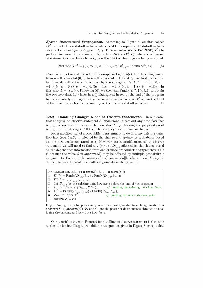
HandleObserve(òld : observe(E), `new : observe(E ′))1: Ddiff = PreIn(Dòld , òld) \ PreIn(Dòld , `new);

2: Γ diff =⋃〈σ,γσ〉∈Ddiff γσ;

3: Let Dènd be the existing data-flow facts before the end of the program;

4: Ψ1=IncUpdate](Dènd , Γdiff ); // handling the existing data-flow facts

5: D∆ = PreIn(Dòld , `new) \ PreIn(Dòld , òld);6: Ψ2=IncProp(D∆); // handling the new data-flow facts7: return Ψ1 ∪ Ψ2;

Fig. 9. An algorithm for performing incremental analysis due to a change made fromobserve(E) to observe(E ′). Ψ1 and Ψ2 are the posterior distributions obtained in ana-lyzing the existing and new data-flow facts.

Our algorithm given in Figure 9 for handling an observe statement is the sameas the one for handling a probabilistic assignment given in Figure 8, except that


IncUpdate in Figure 8 is replaced by IncUpdate] in order to deal with exist-ing data-flow facts in Dènd . Unlike IncUpdate, which uses the seeds in Scom

collected from only one probabilistic assignment ` (modified), IncUpdate] usesΓ diff , which contains a set of single-path dependences possibly from multipleprobabilistic assignments based on the data-flow facts in Ddiff that exist in theoriginal program but not the modified program (lines 1–2).

At line 5, IncProp is reused based on (6) to propagate the new data-flowfacts that were filtered out by the original observe statement but become validafter the change. At line 6, we obtain the new posterior probability distributionsat ènd by combining the results from incremental update and propagation.

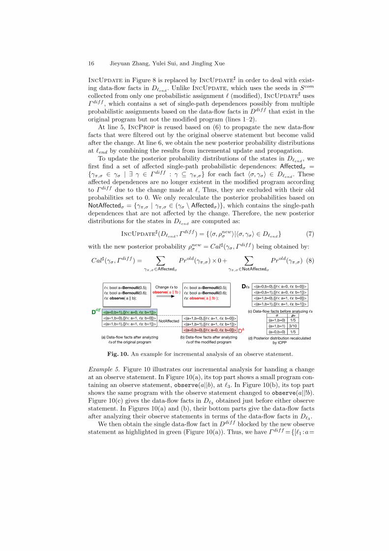
To update the posterior probability distributions of the states in Dènd , wefirst find a set of affected single-path probabilistic dependences: Affectedσ =γπ,σ ∈ γσ | ∃ γ ∈ Γ diff : γ ⊆ γπ,σ for each fact 〈σ, γσ〉 ∈ Dènd . Theseaffected dependences are no longer existent in the modified program accordingto Γ diff due to the change made at `, Thus, they are excluded with their oldprobabilities set to 0. We only recalculate the posterior probabilities based onNotAffectedσ = γπ,σ | γπ,σ ∈ (γσ \ Affectedσ), which contains the single-pathdependences that are not affected by the change. Therefore, the new posteriordistributions for the states in Dènd are computed as:

IncUpdate](Dènd , Γdiff ) = 〈σ, ρnewσ 〉|〈σ, γσ〉 ∈ Dènd (7)

with the new posterior probability ρnewσ = Cal](γσ, Γdiff ) being obtained by:

Cal](γσ, Γdiff ) =

∑γπ,σ∈Affectedσ

Prold(γπ,σ)× 0 +∑

γπ,σ∈NotAffectedσ

Prold(γπ,σ) (8)

D

<(a=1,b=1),[ℓ1: a=1, ℓ2: b=1]><(a=1,b=0),[ℓ1: a=1, ℓ2: b=0]><(a=0,b=1),[ℓ1: a=0, ℓ2: b=1]>

<(a=0,b=0),[ℓ1: a=0, ℓ2: b=0]><(a=1,b=1),[ℓ1: a=1, ℓ2: b=1]><(a=1,b=0),[ℓ1: a=1, ℓ2: b=0]>

ℓ1: bool a=Bernoulli(0.5);ℓ2: bool a=Bernoulli(0.6);ℓ3: observe( a || b);

ℓ1: bool a=Bernoulli(0.5);ℓ2: bool a=Bernoulli(0.6);ℓ3: observe( a || !b );

D

NotAffected

Change ℓ3 toobserve( a || !b )

(a) Data-flow facts after analyzing ℓ3 of the original program

diff

!

(b) Data-flow facts after analyzing ℓ3 of the modified program

<(a=1,b=0),[ℓ1: a=1, ℓ2: b=0]>

<(a=0,b=0),[ℓ1: a=0, ℓ2: b=0]><(a=0,b=1),[ℓ1: a=0, ℓ2: b=1]>

<(a=1,b=1),[ℓ1: a=1, ℓ2: b=1]>

Dℓ3

" #"

3/101/5

1/5(a=0,b=0)(a=1,b=1)(a=1,b=0)

(d) Posterior distribution recalculated by ICPP

(c) Data-flow facts before analyzing ℓ3

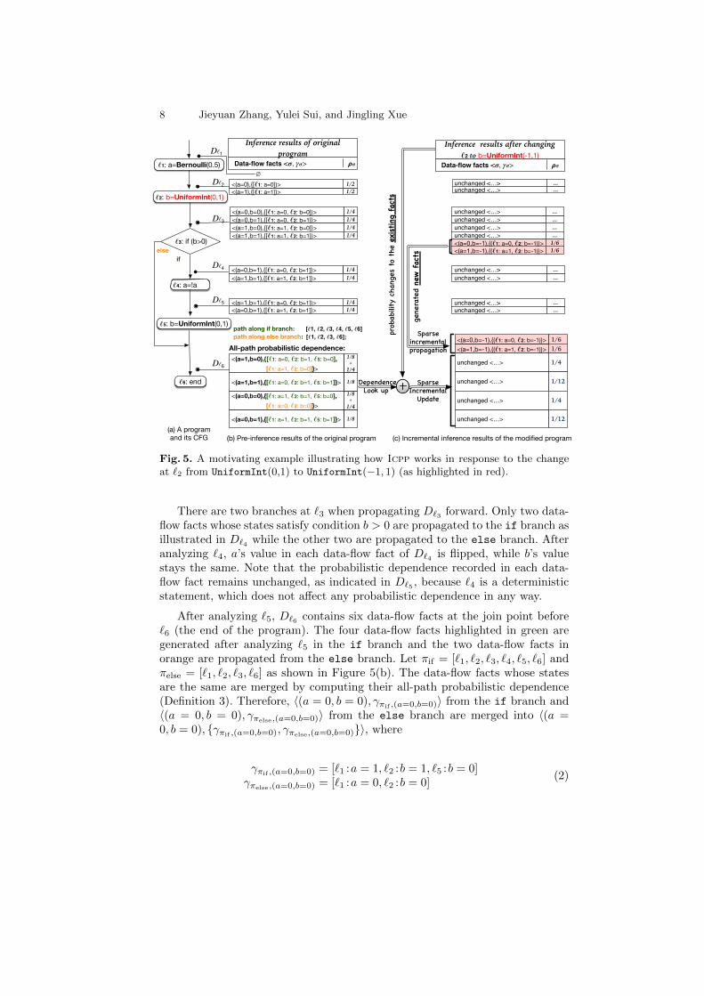
Fig. 10. An example for incremental analysis of an observe statement.

Example 5. Figure 10 illustrates our incremental analysis for handing a changeat an observe statement. In Figure 10(a), its top part shows a small program con-taining an observe statement, observe(a||b), at `3. In Figure 10(b), its top partshows the same program with the observe statement changed to observe(a||!b).Figure 10(c) gives the data-flow facts in D`3 obtained just before either observestatement. In Figures 10(a) and (b), their bottom parts give the data-flow factsafter analyzing their observe statements in terms of the data-flow facts in D`3 .

We then obtain the single data-flow fact in Ddiff blocked by the new observestatement as highlighted in green (Figure 10(a)). Thus, we have Γ diff =[`1 :a=


0, `2 : b= 1], Affectedσ=[`1 :a= 0, `2 : b= 1], and NotAffectedσ=[`1 :a= 1, `2 :b=0], [`1 :a=1, `2 :b=1]. Based on (8), we recalculate the posterior probabilityof each state as ρnew(a=0,b=1) = Pr([`1 :a=0, `2 :b=1])×0 = 0, ρnew(a=1,b=0) = Pr([`1 :

a=1, `2 :b=0]) = 1/5, and ρnew(a=1,b=1) = Pr([`1 :a=1, `2 :b=1]) = 3/10.

The data-flow fact in D∆ as highlighted in red in Figure 10(b) is a new oneintroduced by the change. Finally, we combine the computed probabilities of theexisting and new data-flow facts to obtain the posterior probability distributionsgiven in Figure 10(d). Note that 1/5 + 3/10 + 1/5 6= 1 due to the observestatement. Thus, after having computed the posterior probabilities as desired,we normalize these probabilities as 2/7, 3/7 and 2/7, respectively.

4.3 Precision

Theorem 1. Icpp achieves the same precision as DFI [8] (which analyzes aprogram from scratch) in terms of answering posterior probability distributionsunder the changes made to the probabilistic knowledge of a probabilistic program.

Proof. The pre-inference of Icpp (Figure 6) captures the all-path dependence(Definition 3) of each data-flow fact in order to allow the posterior probabilitydistributions to be updated during the incremental analysis. Every loop in theprogram is handled by approximating a KL-divergence between its two consecutiveloop iterations. A continuous prior distribution is approximated by a discretedistribution over a finite set, following [8,21].

Based on the dependence information, our incremental sparse update recal-culates the posterior probability of any existing data-flow fact affected by anychange to a probabilistic assignment based on (4) or an observe statement basedon (7) while keeping the probabilities of unaffected dependences unchanged. Ourincremental sparse propagation computes and propagates any new data-flow factintroduced by the changes along the CFG based on (6). Following the algorithmsin Figures 8 and 9, we can obtain the same posterior probability distributions asthe program is reanalyzed entirely by DFI (or our pre-inference).

5 Evaluation

Our objective is to demonstrate that Icpp is effective in inferring the posteriordistributions incrementally in response to small yet frequent changes made to aprobabilistic program. Icpp is an order of magnitude faster than DFI [8], a state-of-the-art data-flow-based inference. Our experiment is conducted on a 2.70 GHzIntel Core i5 processor system with 8 GB RAM running macOS.10.12.4.

We have implemented Icpp in Soot [34], a Java analysis framework. Wechoose Figaro [27] as our probabilistic language, which is based on Scala and canbe translated into the .class format for our analysis in Soot. Following DFI [8],we use the ADD library [30] to store our data-flow facts, i.e., probabilistic depen-dences over states, with each single-path dependence naturally represented by anADD. Updating data-flow facts affected by changes to probabilistic assignmentsand observe statements is done by the graph operations in ADD.


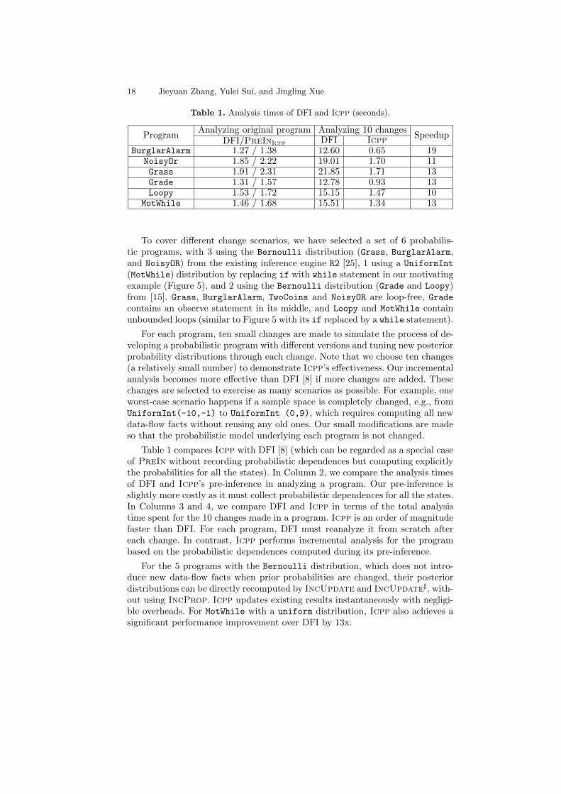
Table 1. Analysis times of DFI and Icpp (seconds).

ProgramAnalyzing original program Analyzing 10 changes

SpeedupDFI/PreInIcpp DFI Icpp

BurglarAlarm 1.27 / 1.38 12.60 0.65 19NoisyOr 1.85 / 2.22 19.01 1.70 11Grass 1.91 / 2.31 21.85 1.71 13Grade 1.31 / 1.57 12.78 0.93 13Loopy 1.53 / 1.72 15.15 1.47 10

MotWhile 1.46 / 1.68 15.51 1.34 13

To cover different change scenarios, we have selected a set of 6 probabilis-tic programs, with 3 using the Bernoulli distribution (Grass, BurglarAlarm,and NoisyOR) from the existing inference engine R2 [25], 1 using a UniformInt

(MotWhile) distribution by replacing if with while statement in our motivatingexample (Figure 5), and 2 using the Bernoulli distribution (Grade and Loopy)from [15]. Grass, BurglarAlarm, TwoCoins and NoisyOR are loop-free, Gradecontains an observe statement in its middle, and Loopy and MotWhile containunbounded loops (similar to Figure 5 with its if replaced by a while statement).

For each program, ten small changes are made to simulate the process of de-veloping a probabilistic program with different versions and tuning new posteriorprobability distributions through each change. Note that we choose ten changes(a relatively small number) to demonstrate Icpp’s effectiveness. Our incrementalanalysis becomes more effective than DFI [8] if more changes are added. Thesechanges are selected to exercise as many scenarios as possible. For example, oneworst-case scenario happens if a sample space is completely changed, e.g., fromUniformInt(-10,-1) to UniformInt (0,9), which requires computing all newdata-flow facts without reusing any old ones. Our small modifications are madeso that the probabilistic model underlying each program is not changed.

Table 1 compares Icpp with DFI [8] (which can be regarded as a special caseof PreIn without recording probabilistic dependences but computing explicitlythe probabilities for all the states). In Column 2, we compare the analysis timesof DFI and Icpp’s pre-inference in analyzing a program. Our pre-inference isslightly more costly as it must collect probabilistic dependences for all the states.In Columns 3 and 4, we compare DFI and Icpp in terms of the total analysistime spent for the 10 changes made in a program. Icpp is an order of magnitudefaster than DFI. For each program, DFI must reanalyze it from scratch aftereach change. In contrast, Icpp performs incremental analysis for the programbased on the probabilistic dependences computed during its pre-inference.

For the 5 programs with the Bernoulli distribution, which does not intro-duce new data-flow facts when prior probabilities are changed, their posteriordistributions can be directly recomputed by IncUpdate and IncUpdate], with-out using IncProp. Icpp updates existing results instantaneously with negligi-ble overheads. For MotWhile with a uniform distribution, Icpp also achieves asignificant performance improvement over DFI by 13x.


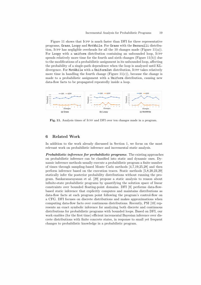
Figure 11 shows that Icpp is much faster than DFI for three representativeprograms, Grass, Loopy and MotWhile. For Grass with the Bernoulli distribu-tion, Icpp has negligible overheads for all the 10 changes made (Figure 11(a)).For Loopy with a uniform distribution containing an unbounded loop, Icppspends relatively more time for the fourth and sixth changes (Figure 11(b)) dueto the modifications of a probabilistic assignment in its unbounded loop, affectingthe probability of a single-path dependence when the loop is analyzed until KL-divergence. For MotWhile with a UniformInt distribution, Icpp takes relativelymore time in handling the fourth change (Figure 11(c)), because the change ismade to a probabilistic assignment with a Uniform distribution, causing newdata-flow facts to be propagated repeatedly inside a loop.

(a) Grass (b) Loopy (c) MotWhile

050010001500200025003000

1 2 3 4 5 6 7 8 9 10

Time(ms)

Changes

DFI ICPP

0

500

1000

1500

2000

1 2 3 4 5 6 7 8 9 10

Time(ms)

Changes

DFI ICPP

0500100015002000250030003500

1 2 3 4 5 6 7 8 9 10

Time(ms)

Changes

DFI ICPP

Fig. 11. Analysis times of Icpp and DFI over ten changes made in a program.

6 Related Work

In addition to the work already discussed in Section 1, we focus on the mostrelevant work on probabilistic inference and incremental static analysis.

Probabilistic inference for probabilistic programs. The existing approacheson probabilistic inference can be classified into static and dynamic ones. Dy-namic inference methods usually execute a probabilistic program a finite numberof times through sampling-based Monte Carlo methods [4,7,19,25,28] and thenperform inference based on the execution traces. Static methods [5,8,20,23,29]statically infer the posterior probability distributions without running the pro-gram. Sankaranarayanan et al. [29] propose a static analysis to reason aboutinfinite-state probabilistic programs by quantifying the solution space of linearconstraints over bounded floating-point domains. DFI [8] performs data-flow-based static inference that explicitly computes and maintains distributions asdata-flow facts at each program point following the program’s control-flow ona CFG. DFI focuses on discrete distributions and makes approximations whencomputing data-flow facts over continuous distributions. Recently, PSI [10] rep-resents an exact symbolic inference for analyzing both discrete and continuousdistributions for probabilistic programs with bounded loops. Based on DFI, ourwork enables (for the first time) efficient incremental Bayesian inference over dis-crete distributions with finite concrete states, in response to small yet frequentchanges to probabilistic knowledge in a probabilistic program.


Incremental static analysis for usual programs. The goal of incrementalstatic analysis is to efficiently update existing analysis results without recom-puting them from scratch, allowing the previously computed information to bereused. Emu [18,31] represents an incremental analysis for performing demand-driven context-sensitive pointer analysis based on Context-Free Language (CFL)reachability, which precisely recomputes points-to sets affected by the programchanges. Reviser [1] is an incremental analysis technique developed as an exten-sion to the IDE-/IFDS- based framework for efficiently updating inter-proceduraldata-flow analysis results. Echo [38] is an incremental analysis for data-racedetection based on program dependences computed by static happens-beforeanalysis. DiSE [26] is an incremental symbolic execution technique that usespre-computed results from a static analysis to direct symbolic execution for ex-ploring only the parts of a program affected by the changes. Unlike previousincremental analysis techniques for imperative programs emphasizing on codechanges, i.e., statement addition and deletion, Icpp focuses on changes made toprobabilistic knowledge, the key feature in probabilistic programming.

7 Conclusion and Future work

In this paper, we present Icpp, a new data-flow based incremental analysis foranalyzing probabilistic programs. Icpp captures the correlation relation betweenprior and posterior probability distributions through a probabilistic dependenceanalysis. The resulting analysis significantly improves the efficiency of data-flowbased inference by incrementally updating the posterior distributions with previ-ous computed information being reused in response to small yet frequent changesmade to probabilistic knowledge, i.e., prior distributions and observations.

This work has opened up some new research opportunities. We can extendour incremental analysis for probabilistic programs by combining it with tradi-tional incremental analyses for usual programs via demand-driven [31,32] and/orpartial program analysis [9,33] in order to also handle the changes made to usualstatements. In addition, we can combine our incremental inference with symbolicanalysis [10,29] to support incremental symbolic inference with hybrid discreteand continuous distributions being supported.

Acknowledgments The authors wish to thank the anonymous reviewers fortheir valuable comments. The first author would like to thankAleksandar Chakarov for some helpful email discussions. This work is supportedby Australian Research Grants, DP150102109, DP170103956 and DE170101081.

References

1. S. Arzt and E. Bodden. Reviser: efficiently updating IDE-/IFDS-based data-flowanalyses in response to incremental program changes. In Proceedings of the 36thInternational Conference on Software Engineering, pages 288–298, 2014.


2. J. Borgstrom, A. D. Gordon, M. Greenberg, J. Margetson, and J. Van Gael. Mea-sure transformer semantics for Bayesian machine learning. In European Symposiumon Programming, pages 77–96, 2011.

3. A. Caticha, A. Giffin, and A. Mohammad-Djafari. Updating probabilities. InInternational Conference on Artificial Intelligence and Pattern Recognition, pages31–42, 2006.

4. A. T. Chaganty, A. V. Nori, and S. K. Rajamani. Efficiently sampling probabilisticprograms via program analysis. In Artificial Intelligence and Statistics, pages 153–160, 2013.

5. A. Chakarov and S. Sankaranarayanan. Expectation invariants for probabilisticprogram loops as fixed points. In International Static Analysis Symposium, pages85–100, 2014.

6. H. Chan and A. Darwiche. On the revision of probabilistic beliefs using uncertainevidence. Artificial Intelligence, 163(1):67–90, 2005.

7. S. Chib and E. Greenberg. Understanding the metropolis-hastings algorithm. Theamerican statistician, 49(4):327–335, 1995.

8. G. Claret, S. K. Rajamani, A. V. Nori, A. D. Gordon, and J. Borgstrom. Bayesianinference using data flow analysis. In Proceedings of the 9th Joint Meeting onFoundations of Software Engineering, pages 92–102, 2013.

9. X. Fan, Y. Sui, X. Liao, and J. Xue. Boosting the precision of virtual call in-tegrity protection with partial pointer analysis for C++. 26th ACM SIGSOFTInternational Symposium on Software Testing and Analysis, 2017.

10. T. Gehr, S. Misailovic, and M. Vechev. PSI: Exact symbolic inference for prob-abilistic programs. In International Conference on Computer Aided Verification,pages 62–83, 2016.

11. P. W. Glynn and D. L. Iglehart. Importance sampling for stochastic simulations.Management Science, 35(11):1367–1392, 1989.

12. A. D. Gordon, T. A. Henzinger, A. V. Nori, and S. K. Rajamani. Probabilisticprogramming. In Proceedings of the on Future of Software Engineering, pages167–181, 2014.

13. W. K. Hastings. Monte carlo sampling methods using markov chains and theirapplications. Biometrika, 57(1):97–109, 1970.

14. M. Hermenegildo, G. Puebla, K. Marriott, and P. J. Stuckey. Incremental analysisof constraint logic programs. ACM Transactions on Programming Languages andSystems, 22(2):187–223, 2000.

15. C.-K. Hur, A. V. Nori, S. K. Rajamani, and S. Samuel. Slicing probabilistic pro-grams. In Proceedings of the 35th ACM SIGPLAN Conference on ProgrammingLanguage Design and Implementation, pages 133–144, 2014.

16. D. Koller and N. Friedman. Probabilistic graphical models: principles and tech-niques. 2009.

17. S. Kullback. Information theory and statistics. 1997.18. Y. Lu, L. Shang, X. Xie, and J. Xue. An incremental points-to analysis with CFL-

reachability. In International Conference on Compiler Construction, pages 61–81,2013.

19. D. J. MacKay. Introduction to monte carlo methods. In Learning in graphicalmodels, pages 175–204. 1998.

20. P. Mardziel, S. Magill, M. Hicks, and M. Srivatsa. Dynamic enforcement ofknowledge-based security policies using probabilistic abstract interpretation. Jour-nal of Computer Security, 21(4):463–532, 2013.

21. A. C. Miller III and T. R. Rice. Discrete approximations of probability distribu-tions. Management science, 29(3):352–362, 1983.


22. T. P. Minka. Expectation propagation for approximate bayesian inference. InProceedings of the Seventeenth conference on Uncertainty in artificial intelligence,pages 362–369, 2001.

23. D. Monniaux. Abstract interpretation of probabilistic semantics. In Proceedingsof the 7th International Symposium on Static Analysis, pages 322–339, 2000.

24. K. P. Murphy, Y. Weiss, and M. I. Jordan. Loopy belief propagation for approx-imate inference: An empirical study. In Proceedings of the 15th Conference onUncertainty in Artificial Intelligence, pages 467–475, 1999.

25. A. V. Nori, C.-K. Hur, S. K. Rajamani, and S. Samuel. R2: An efficient mcmcsampler for probabilistic programs. In Proceedings of the 29th National Conferenceon Artificial Intelligence, pages 2476–2482, 2014.

26. S. Person, G. Yang, N. Rungta, and S. Khurshid. Directed incremental symbolicexecution. In Proceedings of the 32rd ACM SIGPLAN Conference on ProgrammingLanguage Design and Implementation, pages 504–515, 2011.

27. A. Pfeffer. Figaro: An object-oriented probabilistic programming language. CharlesRiver Analytics Technical Report, 137:96, 2009.

28. M. Plummer et al. Jags: A program for analysis of bayesian graphical models usinggibbs sampling. In Proceedings of the 3rd international workshop on distributedstatistical computing, page 125, 2003.

29. S. Sankaranarayanan, A. Chakarov, and S. Gulwani. Static analysis for proba-bilistic programs: inferring whole program properties from finitely many paths. InProceedings of the 34th ACM SIGPLAN Conference on Programming LanguageDesign and Implementation, pages 447–458, 2013.

30. S. Sanner and D. McAllester. Affine algebraic decision diagrams (AADDs) andtheir application to structured probabilistic inference. In Proceedings of the 19thInternational Joint Conference on Artificial Intelligence, pages 1384–1390, 2005.

31. L. Shang, Y. Lu, and J. Xue. Fast and precise points-to analysis with incrementalCFL-reachability summarisation: preliminary experience. In Proceedings of the27th IEEE/ACM International Conference on Automated Software Engineering,pages 270–273, 2012.

32. Y. Sui and J. Xue. On-demand strong update analysis via value-flow refinement. InProceedings of the 2016 24th ACM SIGSOFT International Symposium on Foun-dations of Software Engineering, pages 460–473, 2016.

33. Y. Sui and J. Xue. SVF: Interprocedural static value-flow analysis in LLVM. InProceedings of the 25th International Conference on Compiler Construction, pages265–266, 2016.

34. R. Vallee-Rai, P. Co, E. Gagnon, L. Hendren, P. Lam, and V. Sundaresan. Soot -a Java bytecode optimization framework. In Proceedings of the conference of theCentre for Advanced Studies on Collaborative research, page 13, 1999.

35. M. J. Wainwright, M. I. Jordan, et al. Graphical models, exponential families, andvariational inference. Foundations and Trends R© in Machine Learning, 1(1–2):1–305, 2008.

36. C. Wanke and D. Greenbaum. Incremental, probabilistic decision making for enroute traffic management. Air Traffic Control Quarterly, 15(4):299–319, 2007.

37. A. Yue and W. Liu. Revising imprecise probabilistic beliefs in the framework ofprobabilistic logic programming. In Proceedings of the 23rd National Conferenceon Artificial Intelligence, pages 590–596, 2008.

38. S. Zhan and J. Huang. ECHO: instantaneous in situ race detection in the IDE. InProceedings of the 24th ACM SIGSOFT International Symposium on Foundationsof Software Engineering, pages 775–786, 2016.

Documents

Incremental Analysis for Probabilistic Programs · Incremental Analysis for Probabilistic Programs Jieyuan Zhang 1, Yulei Sui , and Jingling Xue;2 1 School of Computer Science and