Incremental Model-Based Clustering for Large Datasets

With Small Clusters

Chris Fraley ∗, Adrian Raftery‡ and Ron Wehrens†

Technical Report No. 439

Department of StatisticsUniversity of Washington

December 10, 2003

Abstract

Clustering is often useful for analyzing and summarizing information within largedatasets. Model-based clustering methods have been found to be effective for deter-mining the number of clusters, dealing with outliers, and selecting the best clusteringmethod in datasets that are small to moderate in size. For large datasets, currentmodel-based clustering methods tend to be limited by memory and time requirementsand the increasing difficulty of maximum likelihood estimation. They may fit too manyclusters in some portions of the data and/or miss clusters containing relatively few ob-servations. We propose an incremental approach for data that can be processed as awhole in memory, which is relatively efficient computationally and has the ability tofind small clusters in large datasets. The method starts by drawing a random sampleof the data, selecting and fitting a clustering model to the sample, and extending themodel to the full dataset by additional EM iterations. New clusters are then added in-crementally, initialized with the observations that are poorly fit by the current model.We demonstrate the effectiveness of this method by applying it to simulated data, andto image data where its performance can be assessed visually.

Key words: BIC; EM algorithm; Image; MRI.

1 Introduction

The growing size of datasets and databases has led to increased demand for good clustering

methods for analysis and compression, while at the same time introducing constraints in

∗Department of Statistics, University of Washington, Box 354322, Seattle, WA 98195-4322 USA;fraley/raftery@stat.washington.edu

†Department of Analytical Chemistry, University of Nijmegen, Toernooiveld 1, 6525 ED Nijmegen TheNetherlands; rwehrens@sci.kun.nl

1

terms of memory usage and computation time. Model-based clustering, a relatively recent

development (McLachlan and Basford 1988, Banfield and Raftery 1993, McLachlan and Peel

2000, Fraley and Raftery 2002), has shown good performance in many applications on small

to moderate-sized datasets (e.g. Campbell et al. 1997, 1999; Dasgupta and Raftery 1998;

Mukherjee et al. 1998, Yeung et al. 2001; Wang and Raftery 2002; Wehrens et al. 2002).

Direct application of model-based clustering to large datasets is often prohibitively ex-

pensive in terms of computer time and memory. Instead, extensions to large datasets usually

rely on modeling one or more samples of the data, and vary in how the sample-based results

are used to derive a model for all of the data. Underfitting (not enough groups to represent

the data) and overfitting (too many groups in parts of the data) are common problems, in

addition to excessive computational requirements. In this paper we develop an incremental

model-based method that is suitable as a general clustering method for large datasets that

are not too large to be processed as a whole in core (currently up to about 100,000 observa-

tions for a dataset of dimension 10 or less), and is also able to find small clusters if they are

present.

This paper is organized as follows. In Section 2, we give a brief overview of model-based

clustering and introduce the incremental method. In Section 3 we give results for three

large datasets. The first is a large simulated dataset with 14 large clusters and one small

cluster. The remaining two examples are images to be segmented automatically by clustering

information associated with each pixel. One of the images has a prominent feature involving

only a small number of pixels, making segmentation challenging while at the same time

easy to assess visually. The other image is a brain MRI dataset where the task is to find

features of anatomical and clinical interest. In Section 4 we discuss our results and alterative

approaches to the problem.

2 Methods

2.1 Model-Based Clustering

In model-based clustering, the data (x1, . . . ,xn) are assumed to be generated by a mixture

model with densityn

∏

i=1

G∑

k=1

τk fk(xi | θk),

where fk(xi | θk) is a probability distribution with parameters θk, and τk is the probability of

belonging to the kth component or cluster. Most often (and throughout this paper) the fk

are taken to be multivariate normal distributions φk parameterized by their means µk and

2

covariances Σk:

φk(xi | µk, Σk) = |2πΣk|−1/2 exp

{

−1

2(xi − µk)

T Σ−1

k (xi − µk)}

.

The parameters of the model are often estimated by maximum likelihood using the

Expectation-Maximization (EM) algorithm (Dempster et al. 1977; McLachlan and Krishnan

1997). Each EM iteration consists of two steps, an E-step and an M-step. Given an estimate

of the component means µj, covariances Σj and mixing proportions τj, the E-step computes

the conditional probability that object i belongs to cluster k:

zik = φk(xi|µk, Σk)/K

∑

j=1

φj(xi|µj, Σj) .

In the M-step, parameters are estimated from the data given the conditional probabilities zik

(see, e.g., Celeux and Govaert 1995). The E-step and M-step are iterated until convergence,

after which an observation can be assigned to the component or cluster corresponding to the

highest conditional or posterior probability. Good initial values for EM can be obtained effi-

ciently for small to moderate-sized datasets via model-based hierarchical clustering (Banfield

and Raftery 1993; Dasgupta and Raftery 1998; Fraley 1998).

Banfield and Raftery (1993) expressed the covariance matrix for the k-th component or

cluster in the form

Σk = λkDkAkDTk ,

where Dk is the matrix of eigenvectors determining the orientation, Ak is a diagonal matrix

proportional to the eigenvalues determining the shape, and λk is a scalar determining the

volume of the cluster. They used this formulation to define a class of clustering methods

based on cross-cluster geometry, in which mixture components may share a common shape,

volume, and/or orientation. This approach subsumes a number of existing clustering meth-

ods. For example if the clusters are restricted to be spherical and identical in volume, the

clustering criterion is the same as that which underlies Ward’s method (Ward 1963) and

k-means clustering (MacQueen 1967). A detailed description of the 14 different models that

are possible under this scheme can be found in Celeux and Govaert (1995).

Several measures have been proposed for choosing the clustering model (parameterization

and number of clusters); see, e.g., Chapter 6 of McLachlan and Peel (2000). The BIC

approximation to the Bayes factor (Schwarz 1978), which adds a penalty to the loglikelihood

based on the number of parameters, has performed well in a number of applications (e.g.

Dasgupta and Raftery 1998; Fraley and Raftery 1998, 2002).

The following strategy for model-based clustering has been found to be effective for

datasets of up to moderate size:

3

Basic Model-Based Clustering Strategy

1. Determine the minimum and maximum number of clusters to consider (Gmin, Gmax),and a set of candidate parameterizations of the Gaussian model.

2. Do EM for each parameterization and each number of clusters Gmin, . . . , Gmax, start-ing with conditional probabilities corresponding to a classification from unconstrainedmodel-based hierarchical clustering.

3. Compute BIC for the mixture likelihood with the optimal parameters from EM forGmin, . . . , Gmax clusters.

4. Select the model (parameterization / number of clusters) for which BIC is maximized.

For a review of model-based clustering, see Fraley and Raftery (2002).

A limitation of the basic model-based clustering strategy for large datasets is that the

most efficient computational methods for model-based hierarchical clustering have storage

and time requirements that grow at a faster than linear rate relative to the size of the initial

partition, which is usually the set of singleton observations. One straighforward extension

for data that can be processed as a whole in core is to modify step 2 of the basic model-based

clustering strategy modified to do hierarchical clustering only on a sample of the data, rather

than on the whole data set (Fraley and Raftery 1998, 2002). The corresponding parameter

estimates are then used as initial values for EM. We call this method Strategy W.

Strategy W (model from the whole data set)

1. As in the basic model-based clustering strategy.

2. Do EM for each parameterization and each number of clusters Gmin, . . . , Gmax, startingwith parameters obtained from an M-step with conditional probabilities correspondingto a classification from unconstrained model-based hierarchical clustering on a sampleof the data.

3,4. As in the basic model-based clustering strategy.

Strategy W is of limited practical interest because of its excessive computational require-

ments (e.g. Wehrens et al., 2003), and we consider it here only for comparison purposes.

Another sample-based alternative is to apply the basic model-based clustering strategy

to a sample of the data to choose the model and number of clusters, and then extend that

model via EM to the whole of the data (Fraley and Raftery 1998, 2002). We call this method

Strategy S.

4

Strategy S (model from the sample)

1. Apply the basic model-based clustering strategy to a sample of the data.

2. Extend the result to the whole data set via EMa

aExtension is possible via a single E-step or one or more EM iterations.

EM is applied to the full data set only once for a given initial sample in Strategy S, in con-

trast to Strategy W, in which EM is run to convergence on the whole data set for each

model/number of clusters combination.

Wehrens et al. (2003) showed that Strategy S can be improved upon by considering

several candidate models and several EM steps (rather than just one) in the extension to the

full dataset. However, a drawback of Strategy S is that it may miss clusters that are small

but nevertheless significant.

2.2 Incremental Model-Based Clustering

In order to improve on the ability to detect small clusters, we propose an incremental pro-

cedure which starts with a current model (obtained e.g. from Strategy S), and successively

attempts to add new components. EM is initialized with the observations that have the

lowest density under the current model in a separate component, and with the rest of the

observations initially in their current most probable component, and iterated to convergence.

The idea is that the new component would consist largely of observations that are poorly

fit by the current mixture model. The process is terminated after an attempt to add a

component results in no further improvement in BIC.

Strategy I (incremental model-based clustering)

1. Obtain an initial mixture model for the data that underestimates the number of com-ponents (e.g. from Strategy S).

2. Choose a set Q of observations with the lowest densities under the current mixturemodel (e.g. those corresponding to the lowest 1% density).

3. Run one or more steps of EM starting with conditional probabilities corresponding toa discrete classification with observations in Q in a separate group, and the rest of theobservations grouped according to the current model.

4. If step 3 results in a higher BIC, go to step 2.Otherwise fit a less parsimonious model (if possible) starting with the current classifi-ation and go to step 2.

5. If the current model is unconstrained, and BIC decreases in step 4, stop and take thehighest-BIC model to be the solution.

5

The choice of an initial model is required in step 1. In the examples shown here, we

used a model from Strategy S, which is based on model-based hierarchical clustering of a

randomly selected sample of the data, for initialization. We tried several alternatives for

initialization based on random partitions of the data, but the resulting clusterings were not

as good as those from initialization with Strategy S, and had lower BIC values.

In step 2, we used the observations with the lowest 1% of densities under the current

model to initialize the new component. We experimented with other specifications, both

adaptive and nonadaptive, and we found that using the lowest 1% worked as well as or

better than alternatives.

The model change provision in step 3 attempts to preserve parsimony in the model as

much as possible; in practice the algorithm often terminates with an unconstrained covariance

model.

3 Results

Whenever a sample of the data was required in the algorithms, we used a random sample of

size 2000. EM was run to convergence throughout, as defined by a relative tolerance of 10−7

in the loglikelihood.

We used the MCLUST software (Fraley and Raftery 1999, 2004) for both model-based

hierarchical clustering and EM for mixture models. For the image data, only the equal shape

VEV (varying (V) volume, equal (E) shape, and varying (V) orientation) and unconstrained

VVV model were considered, since these seemed to be the only models chosen for these data

(Wehrens et al. 2003).

For examples we use two-dimensional simulated data, as well as two different real image

datasets, to allow visual assessment. Since each method starts by drawing a random sample

of observations from the data, we repeated the computations for 100 different initial samples,

so that our conclusions do not depend on the particular sample drawn.

6

−10 −5 0 5 10

−10

−5

05

10

*

** ****

***

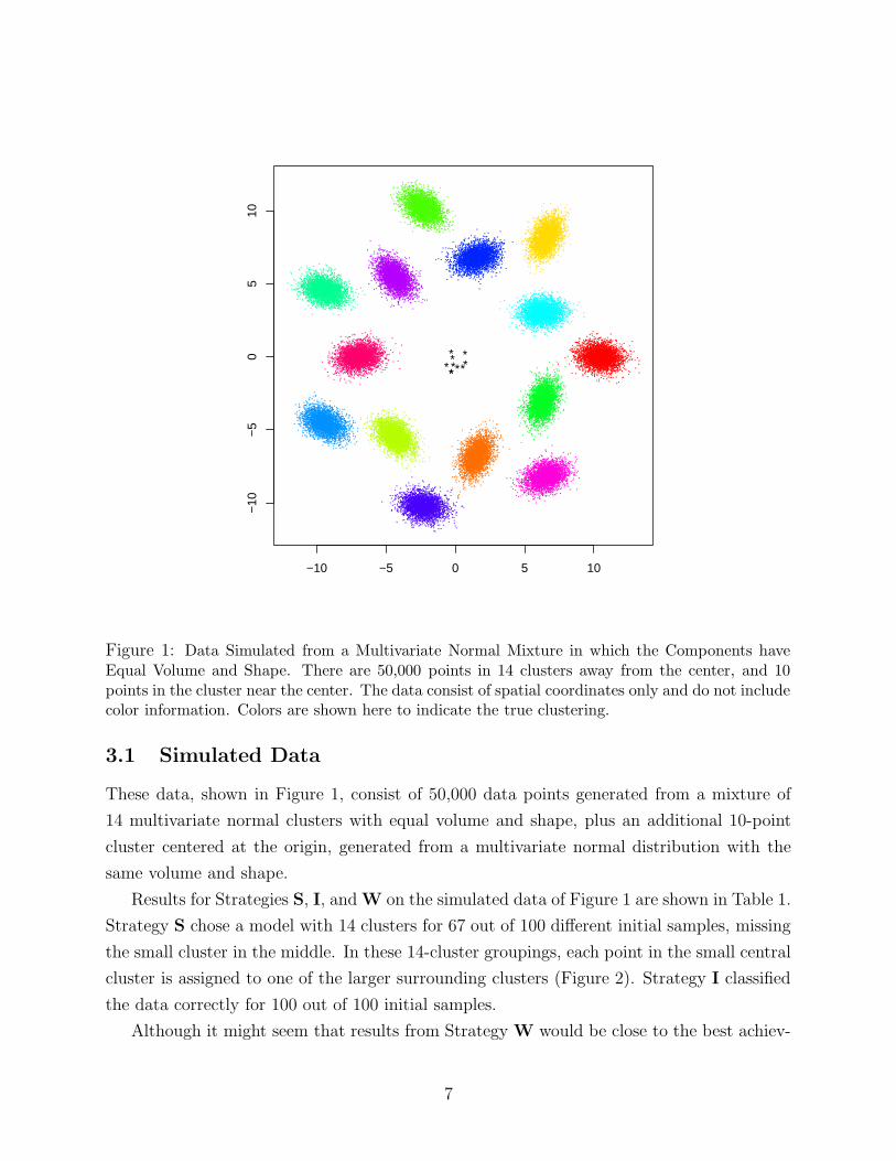
Figure 1: Data Simulated from a Multivariate Normal Mixture in which the Components haveEqual Volume and Shape. There are 50,000 points in 14 clusters away from the center, and 10points in the cluster near the center. The data consist of spatial coordinates only and do not includecolor information. Colors are shown here to indicate the true clustering.

3.1 Simulated Data

These data, shown in Figure 1, consist of 50,000 data points generated from a mixture of

14 multivariate normal clusters with equal volume and shape, plus an additional 10-point

cluster centered at the origin, generated from a multivariate normal distribution with the

same volume and shape.

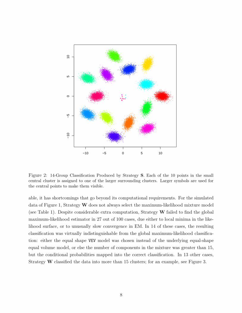
Results for Strategies S, I, and W on the simulated data of Figure 1 are shown in Table 1.

Strategy S chose a model with 14 clusters for 67 out of 100 different initial samples, missing

the small cluster in the middle. In these 14-cluster groupings, each point in the small central

cluster is assigned to one of the larger surrounding clusters (Figure 2). Strategy I classified

the data correctly for 100 out of 100 initial samples.

Although it might seem that results from Strategy W would be close to the best achiev-

7

−10 −5 0 5 10

−10

−5

05

10

*

** ****

***

Figure 2: 14-Group Classification Produced by Strategy S. Each of the 10 points in the smallcentral cluster is assigned to one of the larger surrounding clusters. Larger symbols are used forthe central points to make them visible.

able, it has shortcomings that go beyond its computational requirements. For the simulated

data of Figure 1, Strategy W does not always select the maximum-likelihood mixture model

(see Table 1). Despite considerable extra computation, Strategy W failed to find the global

maximum-likelihood estimator in 27 out of 100 cases, due either to local minima in the like-

lihood surface, or to unusually slow convergence in EM. In 14 of these cases, the resulting

classification was virtually indistinguishable from the global maximum-likelihood classifica-

tion: either the equal shape VEV model was chosen instead of the underlying equal-shape

equal volume model, or else the number of components in the mixture was greater than 15,

but the conditional probabilities mapped into the correct classification. In 13 other cases,

Strategy W classified the data into more than 15 clusters; for an example, see Figure 3.

8

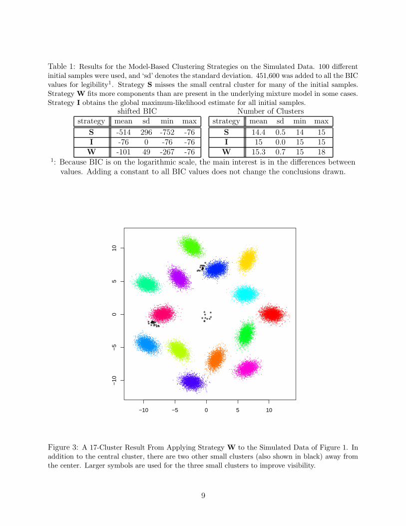
Table 1: Results for the Model-Based Clustering Strategies on the Simulated Data. 100 differentinitial samples were used, and ‘sd’ denotes the standard deviation. 451,600 was added to all the BICvalues for legibility1. Strategy S misses the small central cluster for many of the initial samples.Strategy W fits more components than are present in the underlying mixture model in some cases.Strategy I obtains the global maximum-likelihood estimate for all initial samples.

shifted BIC Number of Clustersstrategy mean sd min max

S -514 296 -752 -76I -76 0 -76 -76W -101 49 -267 -76

strategy mean sd min max

S 14.4 0.5 14 15I 15 0.0 15 15W 15.3 0.7 15 18

1: Because BIC is on the logarithmic scale, the main interest is in the differences betweenvalues. Adding a constant to all BIC values does not change the conclusions drawn.

−10 −5 0 5 10

−10

−5

05

10

*

** ****

***

***

*** * **

****

** *** ***

*****

* ****** ***

Figure 3: A 17-Cluster Result From Applying Strategy W to the Simulated Data of Figure 1. Inaddition to the central cluster, there are two other small clusters (also shown in black) away fromthe center. Larger symbols are used for the three small clusters to improve visibility.

9

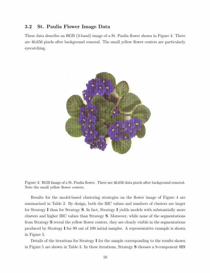
3.2 St. Paulia Flower Image Data

These data describe an RGB (3-band) image of a St. Paulia flower shown in Figure 4. There

are 46,656 pixels after background removal. The small yellow flower centers are particularly

eyecatching.

Figure 4: RGB Image of a St. Paulia flower. There are 46,656 data pixels after background removal.Note the small yellow flower centers.

Results for the model-based clustering strategies on the flower image of Figure 4 are

summarized in Table 2. By design, both the BIC values and numbers of clusters are larger

for Strategy I than for Strategy S. In fact, Strategy I yields models with substantially more

clusters and higher BIC values than Strategy S. Moreover, while none of the segmentations

from Strategy S reveal the yellow flower centers, they are clearly visible in the segmentations

produced by Strategy I for 99 out of 100 initial samples. A representative example is shown

in Figure 5.

Details of the iterations for Strategy I for the sample corresponding to the results shown

in Figure 5 are shown in Table 3. In these iterations, Strategy S chooses a 9-component VEV

10

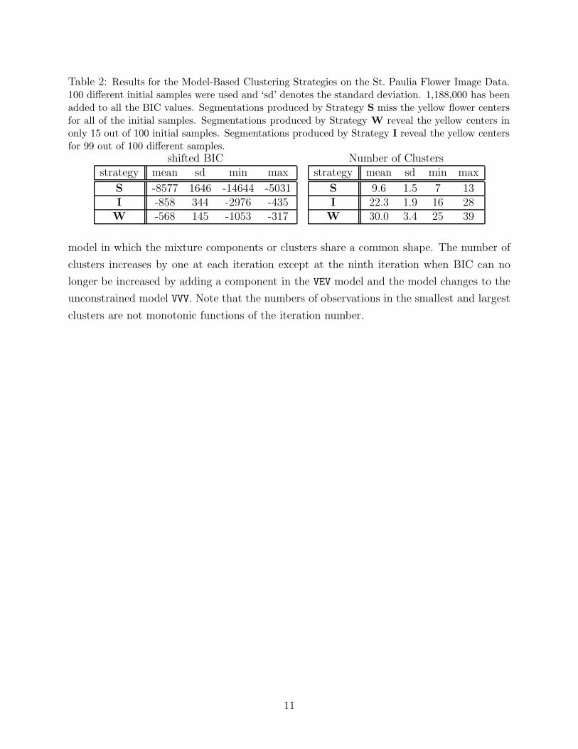
Table 2: Results for the Model-Based Clustering Strategies on the St. Paulia Flower Image Data.100 different initial samples were used and ‘sd’ denotes the standard deviation. 1,188,000 has beenadded to all the BIC values. Segmentations produced by Strategy S miss the yellow flower centersfor all of the initial samples. Segmentations produced by Strategy W reveal the yellow centers inonly 15 out of 100 initial samples. Segmentations produced by Strategy I reveal the yellow centersfor 99 out of 100 different samples.

shifted BIC Number of Clustersstrategy mean sd min max

S -8577 1646 -14644 -5031I -858 344 -2976 -435W -568 145 -1053 -317

strategy mean sd min max

S 9.6 1.5 7 13I 22.3 1.9 16 28W 30.0 3.4 25 39

model in which the mixture components or clusters share a common shape. The number of

clusters increases by one at each iteration except at the ninth iteration when BIC can no

longer be increased by adding a component in the VEV model and the model changes to the

unconstrained model VVV. Note that the numbers of observations in the smallest and largest

clusters are not monotonic functions of the iteration number.

11

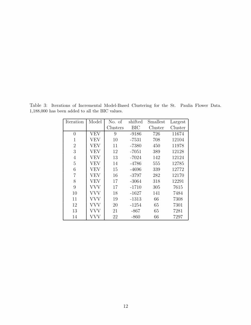
Table 3: Iterations of Incremental Model-Based Clustering for the St. Paulia Flower Data.1,188,000 has been added to all the BIC values.

Iteration Model No. of shifted Smallest LargestClusters BIC Cluster Cluster

0 VEV 9 -9186 726 116741 VEV 10 -7531 708 121042 VEV 11 -7380 450 119783 VEV 12 -7051 389 121284 VEV 13 -7024 142 121245 VEV 14 -4786 555 127856 VEV 15 -4696 339 127727 VEV 16 -3797 282 121708 VEV 17 -3064 318 122919 VVV 17 -1710 305 761510 VVV 18 -1627 141 748411 VVV 19 -1313 66 730812 VVV 20 -1254 65 730113 VVV 21 -867 65 728114 VVV 22 -860 66 7297

12

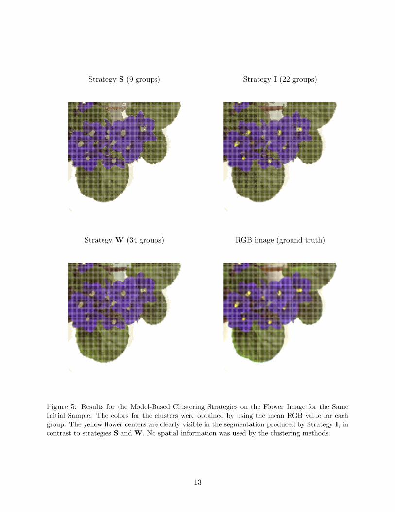
Strategy S (9 groups) Strategy I (22 groups)

Strategy W (34 groups) RGB image (ground truth)

Figure 5: Results for the Model-Based Clustering Strategies on the Flower Image for the SameInitial Sample. The colors for the clusters were obtained by using the mean RGB value for eachgroup. The yellow flower centers are clearly visible in the segmentation produced by Strategy I, incontrast to strategies S and W. No spatial information was used by the clustering methods.

13

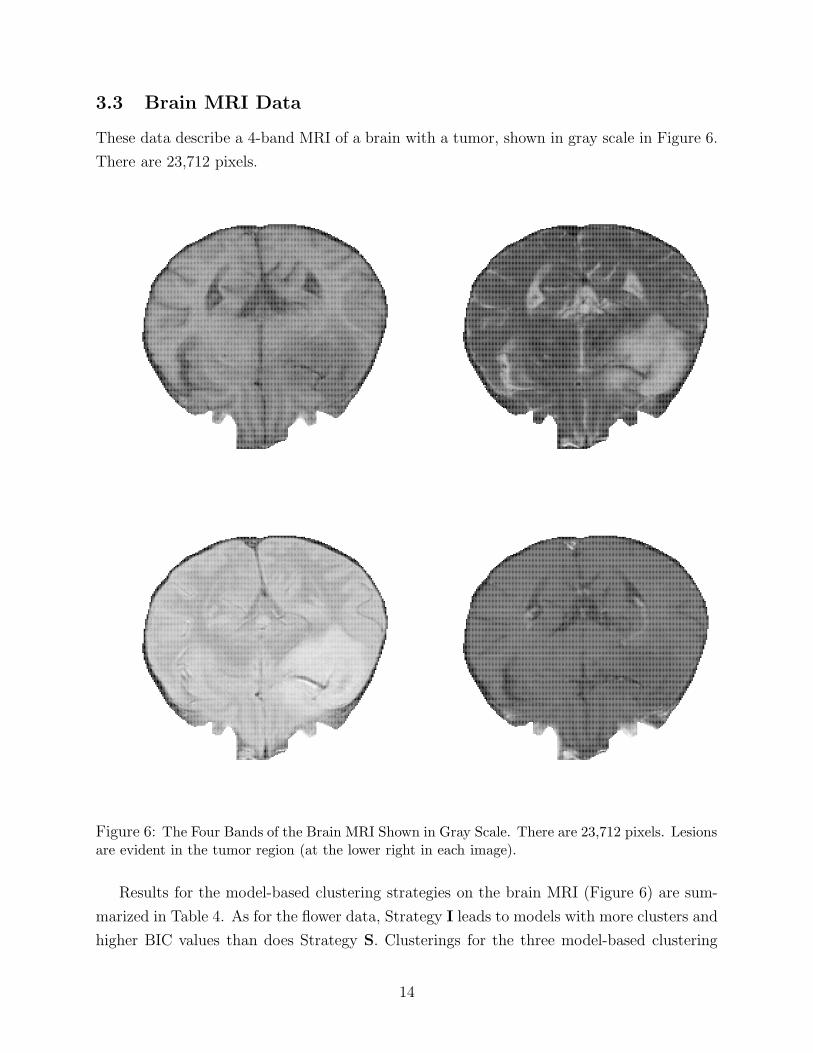
3.3 Brain MRI Data

These data describe a 4-band MRI of a brain with a tumor, shown in gray scale in Figure 6.

There are 23,712 pixels.

Figure 6: The Four Bands of the Brain MRI Shown in Gray Scale. There are 23,712 pixels. Lesionsare evident in the tumor region (at the lower right in each image).

Results for the model-based clustering strategies on the brain MRI (Figure 6) are sum-

marized in Table 4. As for the flower data, Strategy I leads to models with more clusters and

higher BIC values than does Strategy S. Clusterings for the three model-based clustering

14

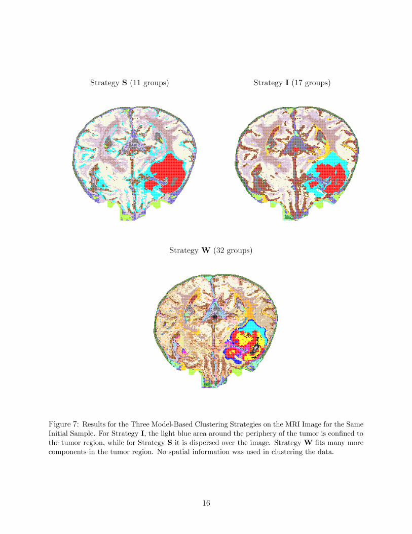
strategies for the same initial sample are shown in Figure 7. In this case the tumor is large

enough to be detected by Strategy S with sample size 2000. One thing to note is that, for

Strategy I, the light blue area at the periphery of the tumor region is confined to the tumor

area, while for Strategy S it is scattered over other regions of the brain. Another observation

is that the segmentation from Strategy I is much smoother and more appealing to the eye

than the fragemented segmentation from Strategy W.

Table 4: Results for the Model-Based Clustering Strategies on the Brain MRI Data. 100 differentinitial samples were used, and ‘sd’ denotes the standard deviation. 755,000 has been added to allthe BIC values.

shifted BIC Number of Clustersstrategy mean sd min max

S -6675 1165 -8601 -3794I -2418 447 -3825 -1658W -867 69 -1025 -670

strategy mean sd min max

S 9.1 1.7 7 14I 17.6 1.7 13 22W 33.7 3.5 26 40

15

Strategy S (11 groups) Strategy I (17 groups)

Strategy W (32 groups)

Figure 7: Results for the Three Model-Based Clustering Strategies on the MRI Image for the SameInitial Sample. For Strategy I, the light blue area around the periphery of the tumor is confined tothe tumor region, while for Strategy S it is dispersed over the image. Strategy W fits many morecomponents in the tumor region. No spatial information was used in clustering the data.

16

4 Discussion

Incremental model-based clustering is a conceptually simple EM-based method that finds

small clusters without subdividing the data into a large number of groups. It can be combined

with any in-core method for improving performance of EM for large datasets. A further

advantage of the incremental approach is that the evolution of the clusters can be monitored

and the process stopped or interrupted as clusters of interest emerge. For complex datasets,

such as the image data shown here, incremental model-based clustering improves on the

ability of the simple sample-based approach to reveal significant small clusters without adding

severely to the computational burden, and without overfitting.

Several other approaches to clustering large datasets based on forming a model from a

sample of the data have been proposed. Fayyad and Smyth (1996) proposed a methodology

for discovering small classes in large datasets, in which a model is first constructed based on

a sample, and then applied to the entire data set. Observations that are well-classified by

the model are retained along with a stratified sample of the rest of the observations, and the

procedure is repeated until all observations are well classified.

Bradley et al. (1998) developed a one-pass (exclusive of sampling) method based on EM

for mixture models that divides the data in to three classes: records that can be discarded

(membership certain), records that can be compressed (known to belong together), and

records that must be retained in memory for further processing (membership uncertain).

Records in the first two classes are represented by their sufficient statistics in subsequent

iterations. Records to be compressed are determined by k-means. Several candidate models

can be updated simultaneously. The number of clusters present in the data is assumed to

be known in advance.

Maitra (2001) proposed a multistage algorithm that clusters an initial sample using a

mixture modeling approach, filters out observations that can be reasonably classified by

these clusters, and iterates the procedure on the remainder. Sample size can be adjusted to

accomodate available computational resources. The procedure requires only a few stages on

very large datasets, but produces many clusters. One reason for the large number of clusters

is the assumption that mixture components have a common covariance, a requirement of the

hypothesis test used to determine representativeness of the identified clusters.

Of course, any sampling-based strategy can be applied to the data for a number of

samples, increasing the chances that a good model for the data will be found. Meek et al.

(2001) give a strategy for determining sample size in methods that extend a sample-based

approach to the full dataset. The basic idea is to apply a training algorithm to larger and

larger subsets of the data, until expected costs outweigh the expected benefits associated

17

with training. The premise is that the best results come from the training algorithm applied

to all of the data. A decision-theoretic framework for cost-benefit analysis is proposed, in

which cost is given in terms of computation time, and benefit or accuracy is the value of the

loglikelihood. Situation and data-dependent scaling issues are discussed. It is assumed that

the number of components in the mixture model is known.

There are also several approaches that are not based on a model derived from a sam-

ple. DuMouchel et al. (1999) proposed strategies for scaling down massive datasets so that

methods for small to moderate sized numbers of observations can be applied. The data

are first grouped into regions, using bins induced by categorical variables and bins induced

either by quantiles or data spheres for quantitative variables. Moments are then calculated

for the elements falling in those regions. Finally, a set of squashed data elements is created

for each region, whose moments approiximate those of the observations in that region. This

produces a smaller dataset to be analyzed which consists of the squashed data elements and

induced weights. The squashed data can then be analyzed by conventional methods that

accept weighted observations. A potential problem is that small clusters may be missed,

although the authors point out that the initial grouping could be constructed in a partially

supervised setting to detect small clusters with known characteristics.

Meek et al. (2002) proposed a stagewise procedure that uses reweighted data to fit a new

component to the current mixture model. As in our method, the new component is accepted

only if it results in an improvement in BIC. Unlike in our method, observations that are

not well-predicted in the current model are given more weight in fitting the new component,

while previous components remain fixed. The authors point out that the method could be

combined with backfitting procedures that could update all components of the model. The

method requires an initial estimate for mixing proportions and model parameters of new

component at each stage, whereas our method starts each stage with a new classification of

the data that separates out observations of low density.

Posse (2001) extended model-based hierarchical clustering to large datasets by using an

initial partition based on the minimum spanning tree. Although the minimum spanning

tree can be computed quickly, it tends to produce groups that are too large to be useful, so

the method is supplemented with strategies for subdividing these groups prior to clustering.

Once an observation is grouped in the initial partition, it cannot be separated from that

group in hierarchical clustering. Also, there are no methods for choosing the number of

clusters in model-based hierarchical clustering that are comparable to those available for

mixture models. However, this approach could be combined with the mixture modeling

approach as a starting scheme for a strategy similar to Strategy W.

Tantrum et al. (2002) extended model-based hierarchical clustering to large data sets

18

through “refractionation”, which splits the data up into many subsets or “fractions”. The

fractions are clustered by model-based hierarchical clustering into a fixed number of groups

and then summarized by their means into meta-observations. These meta-observations are

in turn grouped by model-based clustering, after which a single EM step is applied to the

conditional probabilities defined by the classifications to approximate a mixture likelihood

for computing the BIC, which is used to determine the number of clusters. Initially the data

is divided randomly, but in subsequent iterations, clusters larger than a fixed fraction size

are split into fractions. Observations are assigned to the cluster with the closest mean, and

the procedure is iterated until successive partitions cease to become more similar.

Recently, a number of techniques have become available for speeding up the EM algorithm

on large datasets. Incremental model-based clustering, which relies on the EM algorithm,

can be implemented in combination with any of these. Several of these methods are based

on a partial E-step. In incremental EM (Neal and Hinton 1998; Thiesson et al. 2001),

the E-step is updated in blocks of observations. For normal mixtures, the M-step can be

efficiently implemented to update sufficient statistics in blocks. Lazy EM (McLachlan and

Peel 2000; Thiesson et al. 2001) identifies observations for which the maximum posterior

probability is close to 1 and updates the E-step only for the complement of this subset for

several iterations. A full E-step must be performed periodically to ensure convergence. In

sparse EM (Neal and Hinton 1998), only posterior probabilities above a certain threshold

are updated for each objservation. In the M-step, only the contribution of the sufficient

statistics for the corresponding sufficient statistics need be updated. As for lazy EM, a full

E-step needs to be performed periodically to ensure convergence. Moore (1999) organizes the

data in a multiresolution kd-tree, that allows fast approximations to the E-step in the EM

algorithm by eliminating computations that are considered ignorable. The gain in efficiency

diminishes as the dimension of the data increases. Another approach for large datasets is

a componentwise EM for mixtures (Celeux et al. 2001) in which parameter estimates are

decoupled so as to reduce the size of the missing data space computed in the E-step.

The EM algorithm is well known to have a linear of rate of convergence, which can

sometimes be very slow. Redner and Walker (1984) suggested using a few steps of EM

to start a maximization procedure with faster asymptotic convergence. Methods to speed

up convergence include conjugate-gradient acceleration (Jamshidian and Jennrich 1993),

and Newton approximations, including quasi-Newton methods (Louis 1982; Meilijson 1989;

Lange 1995; Aitken and Aitken 1996; Jamshidian and Jennrich 1997). Although, to the best

of our knowledge, no method of this type has been analyzed with regard to performance on

large datasets, they be might useful in this context from the point of view of reducing the

overall number of iterations as well as for assurance that a local maximum has indeed been

19

reached, the latter being difficult to determine for slow linearly convergent methods.

Acknowledgements

This research was supported by National Institutes of Health grant 8 R01 EB002137–02

and by Office of Naval Research contract contract N00014–01–10745. The authors thank

Christophe Ambroise for thoughtful discussion of this work at the 2003 Session of the Inter-

national Statistical Institute in Berlin.

References

Aitken, M. and I. Aitkin (1996). A hybrid EM/Gauss-Newton algorithm for maximum

likelihood in mixture distributions. Statistics and Computing 6, 127–130.

Banfield, J. D. and A. E. Raftery (1993). Model-based Gaussian and non-Gaussian clus-

tering. Biometrics 49, 803–821.

Bradley, P. S., U. Fayyad, and C. Reina (1998). Scaling clustering algorithms to large

databases. In Proceedings of the Fourth International Conference on Knowledge Dis-

covery and Data Mining (KDD-98). AAAI Press.

Campbell, J. G., C. Fraley, F. Murtagh, and A. E. Raftery (1997). Linear flaw detection

in woven textiles using model-based clustering. Pattern Recognition Letters 18, 1539–

1548.

Campbell, J. G., C. Fraley, D. Stanford, F. Murtagh, and A. E. Raftery (1999). Model-

based methods for real-time textile fault detection. International Journal of Imaging

Systems and Technology 10, 339–346.

Celeux, G., S. Chretien, F. Forbes, and A. Mkhadri (2001). A component-wise EM algo-

rithm for mixtures. Journal of Computational and Graphical Statistics 10, 699–712.

Celeux, G. and G. Govaert (1995). Gaussian parsimonious clustering models. Pattern

Recognition 28, 781–793.

Dasgupta, A. and A. E. Raftery (1998). Detecting features in spatial point processes with

clutter via model-based clustering. Journal of the American Statistical Association 93,

294–302.

Dempster, A. P., N. M. Laird, and D. B. Rubin (1977). Maximum likelihood for incomplete

data via the EM algorithm (with discussion). Journal of the Royal Statistical Society,

Series B 39, 1–38.

20

DuMouchel, W., C. Volinksky, T. Johnson, C. Cortes, and D. Pregibon (1999). Squashing

flat files flatter. In Proceedings of the Fifth International Conference on Knowledge

Discovery and Data Mining (KDD-99). ACM Press.

Fayyad, U. and P. Smyth (1996). From massive data sets to science catalogs: applications

and challenges. In J. Kettenring and D. Pregibon (Eds.), Statistics and Massive Data

Sets: Report to the Committee on Applied and Theoretical Statistics. National Research

Council.

Fraley, C. (1998). Algorithms for model-based Gaussian hierarchical clustering. SIAM

Journal on Scientific Computing 20, 270–281.

Fraley, C. and A. E. Raftery (1998). How many clusters? Which clustering method? -

Answers via model-based cluster analysis. The Computer Journal 41, 578–588.

Fraley, C. and A. E. Raftery (1999). MCLUST: Software for model-based cluster analysis.

Journal of Classification 16, 297–306.

Fraley, C. and A. E. Raftery (2002). Model-based clustering, discriminant analysis and

density estimation. Journal of the American Statistical Association 97, 611–631.

Fraley, C. and A. E. Raftery (2004). Enhanced software for model-based clustering, density

estimation, and discriminant analysis: MCLUST. Journal of Classification.

Jamshidian, M. and R. I. Jennrich (1993). Conjugate gradient acceleration of the EM

algorithm. Journal of the American Statistical Association 88, 221–228.

Jamshidian, M. and R. I. Jennrich (1997). Acceleration of the EM algorithm by using

quasi-Newton methods. Journal of the Royal Statistical Society, Series B 59, 569–587.

Lange, K. (1995). A quasi-Newton acceleration of the EM algorithm. Statistics Sinica 5,

1–18.

Louis, T. A. (1982). Finding the observed information matrix when using the EM algo-

rithm. Journal of the Royal Statistical Society, Series B 44, 226–233.

MacQueen, J. (1967). Some methods for classification and analysis of multivariate ob-

servations. In L. M. L. Cam and J. Neyman (Eds.), Proceedings of the 5th Berkeley

Symposium on Mathematical Statistics and Probability, Volume 1, pp. 281–297. Uni-

versity of California Press.

Maitra, R. (2001). Clustering massive data sets with applications in software metrics and

tomography. Technometrics 43, 336–346.

McLachlan, G. J. and K. E. Basford (1988). Mixture Models : Inference and Applications

to Clustering. Marcel Dekker.

21

McLachlan, G. J. and T. Krishnan (1997). The EM Algorithm and Extensions. Wiley.

McLachlan, G. J. and D. Peel (2000). Finite Mixture Models. Wiley.

Meek, C., B. Thiesson, and D. Heckerman (2001). The learning-curve sampling method

applied to model-based clustering. Journal of Machine Learning Research 2, 397–418.

also in AI and Statistics 2001.

Meek, C., B. Thiesson, and D. Heckerman (2002, August). Staged mixture modeling

and boosting. In Proceedings of Eighteenth Conference on Uncertainty in Artificial

Intelligence, Edmonton, Alberta. Morgan Kaufmann.

Meilijson, I. (1989). A fast improvement of the EM algorithm on its own terms. Journal

of the Royal Statistical Society, Series B 51, 127–138.

Moore, A. (1999). Very fast EM-based mixture model clustering using multiresolution

kd-trees. In M. Kearns, S. Solla, and D. Cohn (Eds.), Advances in Neural Information

Processing Systems, Volume 11, pp. 543–549. MIT Press.

Mukherjee, S., E. D. Feigelson, G. J. Babu, F. Murtagh, C. Fraley, and A. E. Raftery

(1998). Three types of gamma ray bursts. The Astrophysical Journal 508, 314–327.

Neal, R. and G. Hinton (1998). A view of the EM algorithm that justifies incremental,

sparse, and other variants. In M. Jordan (Ed.), Learning in Graphical Models, pp.

355–371. Kluwer.

Posse, C. (2001). Hierarchical model-based clustering for large datasets. Journal of Com-

putational and Graphical Statistics 10, 464–486.

Redner, R. A. and H. F. Walker (1984). Mixture densities, maximum likelihood and the

EM algorithm. SIAM Review 26, 195–239.

Schwarz, G. (1978). Estimating the dimension of a model. The Annals of Statistics 6,

461–464.

Tantrum, J., A. Murua, and W. Stuetzle (2002). Hierarchical model-based clustering of

large datasets through fractionation and refractionation. In Proceedings of the Eighth

International Conference on Knowledge Discovery and Data Mining, pp. 183–190.

ACM Press.

Thiesson, B., C. Meek, and D. Heckerman (2001). Accelerating EM for large datasets.

Machine Learning 45, 279–299.

Wang, N. and A. E. Raftery (2002). Nearest neighbor variance estimation (NNVE): Robust

covarince estimation via nearest neighbor cleaning (with discussion). Journal of the

American Statistical Association 97, 994–1019.

22

Ward, J. H. (1963). Hierarchical groupings to optimize an objective function. Journal of

the American Statistical Association 58, 234–244.

Wehrens, R., L. Buydens, C. Fraley, and A. Raftery (2003, February). Model-based clus-

tering for image segmentation and large datasets via sampling. Technical Report 424,

University of Washington, Department of Statistics.

Wehrens, R., A. Simonetti, and L. Buydens (2002). Mixture-modeling of medical magnetic

resonance data. Journal of Chemometrics 16, 1–10.

Yeung, K. Y., C. Fraley, A. Murua, A. E. Raftery, and W. L. Ruzzo (2001). Model-based

clustering and data transformation for gene expression data. Bioinformatics 17, 977–

987.

23