Indefinite Summation and the Kronecker Delta

Dexter Kozen∗

Cornell UniversityMarc Timme†

Max Planck Institute

October 18, 2007

Abstract

Indefinite summation, together with a generalized version of the Kro-necker delta, provide a calculus for reasoning about various polynomialfunctions that arise in combinatorics, such as the Tutte, chromatic, flow,and reliability polynomials. In this paper we develop the algebraic prop-erties of the indefinite summation operator and the generalized Kroneckerdelta from an axiomatic viewpoint. Our main result is that the axioms areequationally complete; that is, all equations that hold under the intendedinterpretations are derivable in the calculus.

1 Introduction

The indefinite summation operator is very much like a discrete version of anindefinite integral. One can sum an algebraic expression over the values of anunspecified finite set of unspecified size X, and the result is a new expressioninvolving the indeterminate X. The summand may contain symbols δA, for Aa set of variables, a modest generalization of the usual two-variable Kroneckerdelta δxy, which constrain the elements of A all to have the same value.

The interaction of the summation operator∑

x with the δA can be describedwith various algebraic identities. For example,∑

x

(δxyz + δuvδx) = δyz + δuvX.

Intuitively,∑

x δxyz = δyz, because if y and z should have the same value, thenx will take on that value exactly once in the summation, so the constraint thatx, y, z have the same value reduces to the constraint that y and z have the samevalue; and the singleton constraint δx is no constraint at all, so δx = 1, therefore∑

x δuvδx =∑

x δuv = δuvX, where X is the symbolic representation of the sizeof the set of all possible values for x.

∗Computer Science Department, Cornell University, Ithaca, NY 14853-7501, USA.kozen@cs.cornell.edu

†Network Dynamics Group, Max Planck Institute for Dynamics and Self-Organization,Bunsenstrasse 10, 37073 Gottingen, Germany. timme@nld.ds.mpg.de

1

Indefinite summation, together with the generalized Kronecker delta, pro-vide a calculus for reasoning about various polynomial functions that arise ingraph theory, notably the Tutte polynomial and its variants. These polynomialsgive a succinct encoding of a large amount of interesting information about thegraph, such as the number of spanning forests, the number of spanning edge-induced subgraphs, and coloring information. They have a host of applicationsin computer science, mathematics, and physics [15, 10, 3].

Not surprisingly, Tutte polynomials are highly intractable to compute ingeneral. Jaeger et al. [7] show that evaluating the Tutte polynomial at a givenpoint (x, y) is #P -hard except at points on the curve (x − 1)(y − 1) = 1 and8 other special points. Evaluation is tractable in graphs of bounded treewidth[2, 12, 1, 11, 10] but with very large constants. Many of these algorithms arecombinatorial in nature and rely on graph manipulations (e.g. [1]) or reductionsto monadic second-order logic (e.g. [10]).

It is well known that the Tutte polynomial and its variants can be derivedusing summation formulas involving the Kronecker delta δxy. The first use ofthe Kronecker delta in this context seems to be the 1932 paper of Whitney [17],although it was not called by that name. The theory is strongly allied to thetheory of Mobius inversion and incidence algebra [13, 14, 4], and to some extentto the calculus of finite differences [8]. In fact it can be cast as a theory ofcertain linear operators on the Mobius algebra of a semilattice of partitions [6].

Our ultimate goal is to exploit this theory to derive more abstract sym-bolic algorithms for the Tutte polynomial and its variants in special cases, withthe hope that such algorithms might be more efficient or easier to program oranalyze. This paper constitutes an initial step in this direction. We study asystem of polynomials with indefinite summation operators and the general-ized Kronecker delta. We develop the algebraic properties of these constructsfrom an axiomatic viewpoint. Our main result is a complete axiomatizationof their equational theory; that is, all equations that hold under the intendedinterpretations are derivable in the calculus.

This paper is organized as follows. In Section 2, we develop the algebraictheory of the generalized Kronecker delta and prove several basic results. InSection 3, we introduce an axiomatization and prove that it is sound and com-plete with respect to the class of intended interpretations. In Section 4, weintroduce the indefinite summation operator, extend the axiomatization andthe semantics to include summation, and reprove soundness and completeness.Finally, in Section 5, we illustrate the use of the calculus by giving a symbolicderivation of the closed form of the chromatic polynomial.

Our development relies on some elementary concepts from algebra, for whichwe refer the reader to [9, 16].

2 The Kronecker Delta

Let V be a finite set of size n. Let A,B, . . . denote subsets of V . The powersetof V is the set of all subsets of V and is denoted 2V . Let C be another finite

2

set of size m, and let CV denote the set of functions f : V → C. Intuitively,we regard C as a set of colors and a function f : V → C as a coloring of theelements of V . The set CV is the set of all possible colorings.

For A ⊆ V , the Kronecker delta δA is the function δA : CV → {0, 1} definedby:

δA(f) def={

1, if ∀x, y ∈ A f(x) = f(y)0, otherwise. (2.1)

={

1, if A is monochromatic under the coloring f0, otherwise.

This is a modest generalization of the usual Kronecker delta, which is tradition-ally defined only for two-element sets:

δxy(f) def={

1, if f(x) = f(y)0, otherwise.

Here we have written δxy as an abbreviation for δ{x,y}. We will similarly writeδx for δ{x}, δxyz for δ{x,y,z}, etc.

2.1 Axiomatization

The space of functions F : CV → {0, 1} forms a commutative monoid underthe pointwise operations, and the functions δA are elements of this monoid.Multiplication on the δA satisfies all the laws of commutative monoids (associa-tivity, commutativity, and the identity laws), as well as the following additionalproperties.

(2.2) δAδB = δA∪B if A ∩ B 6= ∅

(2.3) δA = 1 if A is either ∅ or a singleton.

Equivalently,

(2.4) δA =∏

B⊆A|B|=2

δB

(2.5) δxyδyz = δxyδyzδxz (transitivity).

Lemma 2.1 Modulo the laws of commutative monoids, (2.2) and (2.3) areequivalent to (2.4) and (2.5).

Proof. We apply the laws of commutative monoids (associativity, commuta-tivity, identity laws) without comment. Suppose (2.2) and (2.3) hold. Property(2.5) follows immediately from three applications of (2.2):

δxyδyz = δxyz = δxyzδxz = δxyδyzδxz.

3

For (2.4), let A = {x1, . . . , xn}, n ≥ 0. If n = 0 or n = 1, then δA = 1 by(2.3), and the right-hand side of (2.4) is also 1 since it is a vacuous product, asthere are no subsets of A of size 2. If n ≥ 2, we can express the right-hand sideof (2.4) as the product

∏i<j δxixj

, then use (2.5) (which we have just proved)to eliminate factors δxixj

in order of decreasing j − i until obtaining a product

δx1x2δx2x3 · · · δxn−1xn .

We then use (2.2) inductively to combine adjacent factors until we obtain δA.Conversely, suppose (2.4) and (2.5) hold. Axiom (2.3) follows from (2.4),

since as noted above, the right-hand side of (2.4) is 1 when |A| ≤ 1. For (2.2),suppose A ∩ B 6= ∅. Picking z = y in (2.5) and using (2.3) (which we have justproved), we have

δxy = δxyδyy = δxyδyyδxy = δ2xy. (2.6)

Then

δA∪B =∏x∈Ay∈A

δxy

∏x∈Ay∈B

δxy

∏x∈By∈B

δxy =∏x∈Ay∈A

δxy

∏x∈By∈B

δxy = δAδB .

The first equation is just (2.4), using (2.6) to obtain the duplicated factors forx or y ∈ A ∩ B. The second follows from several applications of (2.5) to getrid of the middle product, using the fact that A ∩ B 6= ∅. The last is just twoapplications of (2.4). 2

A useful consequence is that if A ⊆ B, then δB = δAδB . This is imme-diate from (2.3) if A = ∅ and (2.2) if A 6= ∅. In particular, multiplication isidempotent : δA = δ2

A for any A. Multiplication in the monoid CV → {0, 1}is idempotent, but it is important to note that we did not use this fact in theproof of Lemma 2.1, but derived the idempotence of the δA axiomatically from(2.2)–(2.3) and (2.4)–(2.5).

2.2 Partitions

A partition of V is a family of pairwise disjoint subsets of V whose union isV . Partitions are denoted π, ρ, . . . . We say that π refines ρ and write π v ρ ifeach set of π is a subset of a set of ρ; equivalently, if each set of ρ is a unionof sets of π. Refinement is a partial order, and every pair of partitions has aleast upper bound with respect to refinement, denoted π t ρ. This is the finestpartition refined by both π and ρ. The v-least element is the identity partitionι = {{x} | x ∈ V } and the v-greatest element is {V }. Thus the family ofpartitions of V forms an upper semilattice Π(V ). It also forms a lattice, themeet operation being coarsest common refinement, but this is not relevant forour purposes.

For any family F ⊆ 2V , define

δFdef=

∏A∈F

δA.

4

Theorem 2.2 The free monoid generated by {δA | A ⊆ V }, modulo (2.2) and(2.3) (or equivalently by Lemma 2.1, (2.4) and (2.5)), is isomorphic to Π(V ),the upper semilattice of partitions of V .

Proof. It follows from the laws of commutative monoids and the axioms(2.2)–(2.3) or (2.4)–(2.5) that every F ⊆ 2V generates a unique partition π ofV such that δF = δπ. We can form π by starting with (F−∅) ∪ {{x} | x 6∈

⋃F},

as justified by (2.2), and replacing A,B such that A ∩ B 6= ∅ with A ∪ B untilno more such steps are possible, as justified by (2.3).

It also follows that δπδρ = δπtρ and π v ρ iff δπδρ = δρ. Also, δι = 1,where ι is the identity partition. Thus the map that takes π to δπ constitutesan isomorphism of monoids. 2

2.3 Normal Form

Let R be a commutative ring. The space of functions F : CV → R also forms acommutative ring under the pointwise operations, and the monoid of functionsCV → {0, 1} embeds faithfully into this ring.

One can also form the polynomial ring R[δA | A ⊆ V ] and its quotientmodulo (2.2)–(2.3) or (2.4)–(2.5). In light of Theorem 2.2, this quotient struc-ture is isomorphic to the semigroup algebra over R of the upper semilattice ofpartitions of V . This structure is known as the Mobius algebra of the semilattice[6]. We will explore this correspondence more fully in Section 3.7.

Lemma 2.3 (Normal Form) Any polynomial expression in R[δA | A ⊆ V ]is equivalent modulo (2.2)–(2.3) or (2.4)–(2.5) to an expression of the form∑

π aπδπ, where aπ ∈ R.

Proof. Multiply out the given expression to obtain a sum of terms of the formaF δF , replace δF by δπ where π is the partition generated by F , and combinelike terms. 2

3 Soundness and Completeness

Let R[δA | A ⊆ V ] denote the ring of polynomials with indeterminates δA,A ⊆ V , and coefficients in R. In this section we show that the axioms (2.2) and(2.3) (equivalently by Lemma 2.1, (2.4) and (2.5)) are equationally sound andcomplete for all interpretations of the δA as functions of the form (2.1). That is,any equation between polynomials in R[δA | A ⊆ V ] that holds under all suchinterpretations is provable by equational logic from the axioms. We will alsoshow that the axioms are complete for interpretations over a fixed color classC, provided |C| ≥ n. Color classes of size less than n require an extra axiom.

Technically, we must include the equational theory of R in our axiomati-zation. In all our applications, R will be either Z or a polynomial ring Z[X]or Q[X]. The equational theory of Z or Z[X] consists of nothing beyondthe axioms of commutative rings, since these are free commutative rings. For

5

Q[X], we must also include arithmetic in Q. The equational theory of R andthe axioms of commutative rings will be part of all our axiomatizations, so wewill take this for granted and not mention it further.

3.1 Notational Preliminaries

To formulate the theorem precisely, we must distinguish between the formalsymbol δA and the function CV → {0, 1} it represents. We will henceforth usethe notation [[δA]]C for the latter.

We will also use the notation Θ(ϕ) for the characteristic function of a propo-sition ϕ, defined by

Θ(ϕ) def={

1, if ϕ0, otherwise.

For a coloring f : V → C, let ρf be the partition on V induced by f−1:

ρfdef= {f−1(c) | c ∈ C, f−1(c) 6= ∅}.

The elements of ρf are the maximal nonempty subsets of V that are monochro-matic under the coloring f .

Similarly, for a set A ⊆ V , let ρA be the partition generated by A, namely{A} ∪ {{x} | x 6∈ A}, or just ι if A = ∅.

With this notation, we can rewrite (2.1) as

[[δA]]C(f) def={

1, if ∀x, y ∈ A f(x) = f(y)0, otherwise

= Θ(∀x, y ∈ A f(x) = f(y))= Θ(ρA v ρf ).

(3.1)

Equation (3.1) defines a set map

[[ ]]C : {δA | A ⊆ V } → (CV → R),

which extends uniquely to a ring homomorphism

[[ ]]C : R[δA | A ⊆ V ] → (CV → R). (3.2)

This is just the evaluation homomorphism that evaluates a given polynomial pby substituting the values [[δA]]C for the indeterminates δA. Under this exten-sion,

[[δπ]]C(f) = Θ(π v ρf ). (3.3)

It is clear from (3.1) and (3.3) that the interpretation [[p]]C : CV → R doesnot depend on the actual colorings f : V → C, but only on the partitions ρf

they generate.

6

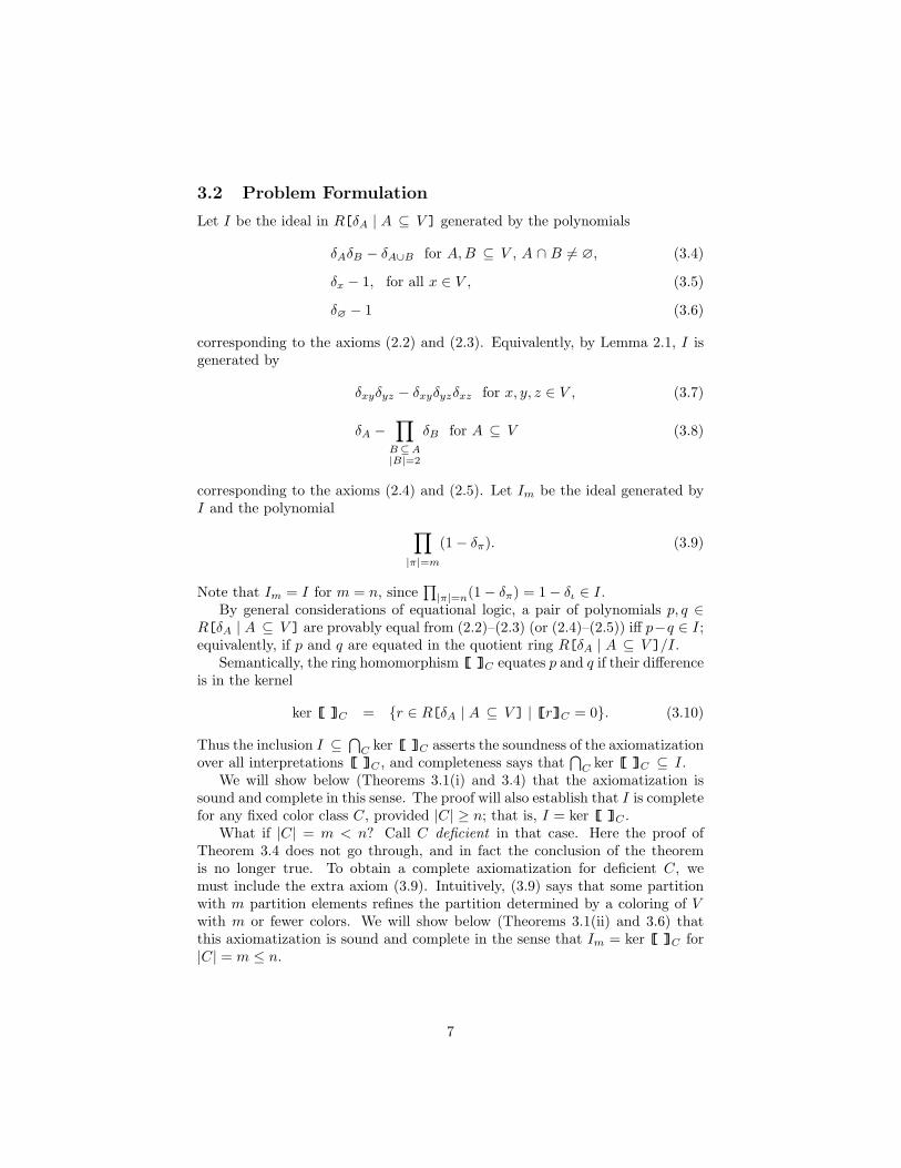
3.2 Problem Formulation

Let I be the ideal in R[δA | A ⊆ V ] generated by the polynomials

δAδB − δA∪B for A,B ⊆ V , A ∩ B 6= ∅, (3.4)

δx − 1, for all x ∈ V , (3.5)

δ∅ − 1 (3.6)

corresponding to the axioms (2.2) and (2.3). Equivalently, by Lemma 2.1, I isgenerated by

δxyδyz − δxyδyzδxz for x, y, z ∈ V , (3.7)

δA −∏

B⊆A|B|=2

δB for A ⊆ V (3.8)

corresponding to the axioms (2.4) and (2.5). Let Im be the ideal generated byI and the polynomial ∏

|π|=m

(1− δπ). (3.9)

Note that Im = I for m = n, since∏|π|=n(1− δπ) = 1− δι ∈ I.

By general considerations of equational logic, a pair of polynomials p, q ∈R[δA | A ⊆ V ] are provably equal from (2.2)–(2.3) (or (2.4)–(2.5)) iff p−q ∈ I;equivalently, if p and q are equated in the quotient ring R[δA | A ⊆ V ]/I.

Semantically, the ring homomorphism [[ ]]C equates p and q if their differenceis in the kernel

ker [[ ]]C = {r ∈ R[δA | A ⊆ V ] | [[r]]C = 0}. (3.10)

Thus the inclusion I ⊆⋂

C ker [[ ]]C asserts the soundness of the axiomatizationover all interpretations [[ ]]C , and completeness says that

⋂C ker [[ ]]C ⊆ I.

We will show below (Theorems 3.1(i) and 3.4) that the axiomatization issound and complete in this sense. The proof will also establish that I is completefor any fixed color class C, provided |C| ≥ n; that is, I = ker [[ ]]C .

What if |C| = m < n? Call C deficient in that case. Here the proof ofTheorem 3.4 does not go through, and in fact the conclusion of the theoremis no longer true. To obtain a complete axiomatization for deficient C, wemust include the extra axiom (3.9). Intuitively, (3.9) says that some partitionwith m partition elements refines the partition determined by a coloring of Vwith m or fewer colors. We will show below (Theorems 3.1(ii) and 3.6) thatthis axiomatization is sound and complete in the sense that Im = ker [[ ]]C for|C| = m ≤ n.

7

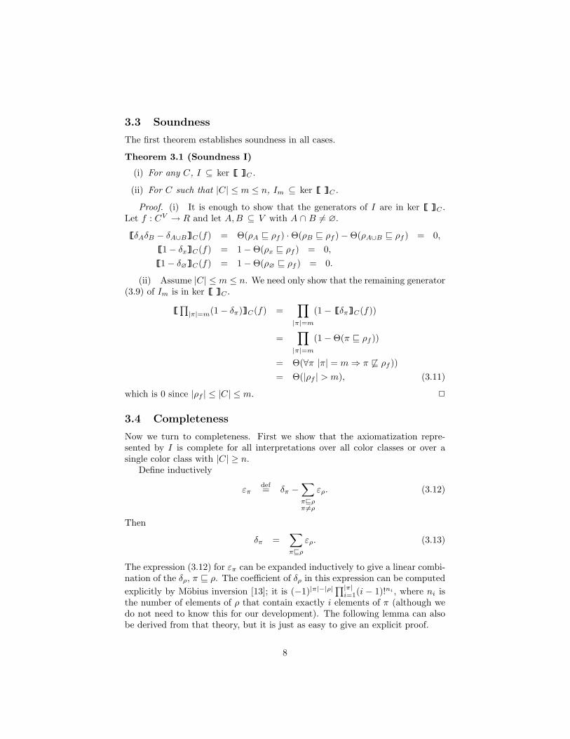
3.3 Soundness

The first theorem establishes soundness in all cases.

Theorem 3.1 (Soundness I)

(i) For any C, I ⊆ ker [[ ]]C .

(ii) For C such that |C| ≤ m ≤ n, Im ⊆ ker [[ ]]C .

Proof. (i) It is enough to show that the generators of I are in ker [[ ]]C .Let f : CV → R and let A,B ⊆ V with A ∩ B 6= ∅.

[[δAδB − δA∪B]]C(f) = Θ(ρA v ρf ) ·Θ(ρB v ρf )−Θ(ρA∪B v ρf ) = 0,

[[1− δx]]C(f) = 1−Θ(ρx v ρf ) = 0,

[[1− δ∅]]C(f) = 1−Θ(ρ∅ v ρf ) = 0.

(ii) Assume |C| ≤ m ≤ n. We need only show that the remaining generator(3.9) of Im is in ker [[ ]]C .

[[∏|π|=m(1− δπ)]]C(f) =

∏|π|=m

(1− [[δπ]]C(f))

=∏

|π|=m

(1−Θ(π v ρf ))

= Θ(∀π |π| = m ⇒ π 6v ρf ))= Θ(|ρf | > m), (3.11)

which is 0 since |ρf | ≤ |C| ≤ m. 2

3.4 Completeness

Now we turn to completeness. First we show that the axiomatization repre-sented by I is complete for all interpretations over all color classes or over asingle color class with |C| ≥ n.

Define inductively

επdef= δπ −

∑πvρπ 6=ρ

ερ. (3.12)

Then

δπ =∑πvρ

ερ. (3.13)

The expression (3.12) for επ can be expanded inductively to give a linear combi-nation of the δρ, π v ρ. The coefficient of δρ in this expression can be computedexplicitly by Mobius inversion [13]; it is (−1)|π|−|ρ|

∏|π|i=1(i − 1)!ni , where ni is

the number of elements of ρ that contain exactly i elements of π (although wedo not need to know this for our development). The following lemma can alsobe derived from that theory, but it is just as easy to give an explicit proof.

8

Lemma 3.2 For all f : V → C, [[επ]]C(f) = Θ(π = ρf ).

Proof. By downward induction on v. Assume that the lemma is true for allρ such that π v ρ, π 6= ρ. Then

[[επ]]C(f) = [[δπ −∑πvρπ 6=ρ

ερ]]C(f)

= [[δπ]]C(f)−∑πvρπ 6=ρ

[[ερ]]C(f)

= Θ(π v ρf )−∑πvρπ 6=ρ

Θ(ρ = ρf )

= Θ(π v ρf )−Θ(π v ρf ∧ π 6= ρf )= Θ(π = ρf ).

2

Lemma 3.3 Let |C| ≥ m. Any polynomial∑

|π|≤m aπδπ or∑

|π|≤m bπεπ thatvanishes under [[ ]]C is identically 0.

Proof. Suppose [[∑

|π|≤m bπεπ]]C = 0. We show by induction on v that allcoefficients bπ are 0. Let |σ| ≤ m and assume bπ = 0 for π v σ, π 6= σ. Weshow that bσ = 0 as well. Let f : CV → R such that ρf = σ. Such an f existsby the assumption |C| ≥ m.

0 = [[∑|π|≤m

bπεπ]]C(f)

=∑|π|≤m

bπΘ(π = σ)

=∑|π|≤mπvσπ 6=σ

bπΘ(π = σ) +∑|π|≤mπ=σ

bπΘ(π = σ) +∑|π|≤mπ 6vσ

bπΘ(π = σ)

= 0 + bσ + 0= bσ.

The result for∑

|π|≤m aπδπ follows from this via (3.12) and (3.13). 2

Theorem 3.4 (Completeness I) For all C such that |C| ≥ n, ker [[ ]]C ⊆ I.

Proof. Let p ∈ R[δA | A ⊆ V ] such that [[p]]C = 0. We wish to showthat p ∈ I. By Lemma 2.3, p is equivalent modulo I to a polynomial

∑π aπδπ,

aπ ∈ R. By Theorem 3.1(i), [[∑

π aπδπ]]C = 0. By Lemma 3.3 with m = n,∑π aπδπ = 0, therefore p ∈ I. 2

9

3.5 Completeness for Deficient C

To prove completeness for deficient color classes, we need one more lemma.

Lemma 3.5 If |π| > m then επ ∈ Im.

Proof. Modulo Im, επ is equivalent to

επ(1−∏|ρ|=m

(1− δρ)), (3.14)

so it suffices to show that (3.14) is in Im. In fact, it is in I. Let |C| ≥ n. Forall f : V → C, by (3.11),

[[1−∏|ρ|=m

(1− δρ)]]C(f) = Θ(|ρf | ≤ m),

and since |π| > m,

[[επ(1−∏|ρ|=m(1− δρ))]]C(f) = [[επ]]C(f) · [[1−

∏|ρ|=m(1− δρ)]]C(f)

= Θ(π = ρf ) ·Θ(|ρf | ≤ m)= 0.

As f was arbitrary, (3.14) is in ker [[ ]]C . By Theorem 3.4, it is in I. 2

Theorem 3.6 (Completeness II) For all C such that |C| ≥ m, ker [[ ]]C ⊆Im.

Proof. The proof is similar to Theorem 3.4. Let p ∈ R[δA | A ⊆ V ] suchthat [[p]]C = 0. We wish to show that p ∈ Im. Combining Lemma 2.3 withLemma 3.5, p is equivalent modulo Im to a polynomial

∑|π|≤m bπεπ, bπ ∈ R.

By Theorem 3.1(ii), [[∑

|π|≤m bπεπ]]C = 0. By Lemma 3.3,∑

|π|≤m bπεπ = 0,therefore p ∈ Im. 2

The following are some consequences of the completeness theorem.

Corollary 3.7 Let m ≤ n and let |π| ≥ m. The following three expressions areall equivalent to δπ modulo Im:

1−∏πvρ|π|=m

(1− δρ) 1−∏πvρ|π|≤m

(1− δρ) 1−∏πvρ|π|≤m

(1− ερ). (3.15)

Proof. Let |C| = m and f : V → C. Then

[[δπ]]C(f) = Θ(π v ρf ). (3.16)

10

Reasoning semantically, the three expressions reduce to

[[1−∏πvρ|ρ|=m

(1− δρ)]]C(f) = Θ(∃ρ π v ρ ∧ |ρ| = m ∧ ρ v ρf ),

[[1−∏πvρ|ρ|≤m

(1− δρ)]]C(f) = Θ(∃ρ π v ρ ∧ |ρ| ≤ m ∧ ρ v ρf ),

[[1−∏πvρ|ρ|≤m

(1− ερ)]]C(f) = Θ(∃ρ π v ρ ∧ |ρ| ≤ m ∧ ρ = ρf )

= Θ(π v ρf ∧ |ρf | ≤ m).

These are all equal to (3.16), since |ρf | ≤ m. As f was arbitrary, the expressions(3.15) are equivalent to δπ under the map [[ ]]C . By completeness, they areequivalent modulo Im. 2

3.6 Dimensionality

We have actually shown

Theorem 3.8

(i) The quotient rings R[δA | A ⊆ V ]/I and R[δA | A ⊆ V ]/ker [[ ]]C for|C| ≥ n are isomorphic R-modules of dimension Bn, the nth Bell number(number of partitions of a set of size n). The sets {επ | π ∈ Π(V )} and{δπ | π ∈ Π(V )} each form a basis.

(ii) The quotient rings R[δA | A ⊆ V ]/Im and R[δA | A ⊆ V ]/ker [[ ]]C

for |C| = m ≤ n are isomorphic R-modules of dimension Bmn , the number

of partitions of a set of size n with at most m partition elements1. Thesets {επ | π ∈ Π(V ), |π| ≤ m} and {δπ | π ∈ Π(V ), |π| ≤ m} each form abasis.

Proof. The statement (i) is a special case of (ii) with m = n.For (ii), it follows from (3.12) and (3.13) that one of {δπ | π ∈ Π(V ), |π| ≤

m} and {επ | π ∈ Π(V ), |π| ≤ m} is a basis if and only if the other is, so weneed only show the latter.

As argued in Theorem 3.6, every polynomial is equivalent modulo Im toone of the form

∑|π|≤m bπεπ, thus R[δA | A ⊆ V ]/Im is an R-module of

dimension at most Bmn spanned by the επ, |π| ≤ m. By Theorem 3.1, there is a

homomorphism of R-modules

h : R[δA | A ⊆ V ]/Im → R[δA | A ⊆ V ]/ker [[ ]]C ,

thus the dimension of R[δA | A ⊆ V ]/ker [[ ]]C is bounded by the dimension ofR[δA | A ⊆ V ]/Im. By Lemma 3.3, the επ for |π| ≤ m are linearly independent

1This isPn

m=0

�nm

, where the

�nm

are Stirling numbers of the second kind [5].

11

modulo ker [[ ]]C , thus the dimension of R[δA | A ⊆ V ]/ker [[ ]]C as an R-module is at least Bm

n . Putting these observations together, we have

Bmn ≤ dim R[δA | A ⊆ V ]/ker [[ ]]C ≤ dim R[δA | A ⊆ V ]/Im ≤ Bm

n ,

therefore all these inequalities are equalities, and the homomorphism h is anisomorphism. 2

3.7 The Mobius Algebra

As mentioned in Section 2.3, the quotient R[δA | A ⊆ V ]/I is isomorphic to thesemigroup algebra of Π(V ), the upper semilattice of partitions of V , over R. Thisis known as the Mobius algebra of the semilattice Π(V ) [6]. Informally, it consistsof linear combinations of elements of Π(V ) with coefficients in R. Formally, itcan be characterized in two ways: (i) as a quotient ring R[δπ | π ∈ Π(V )]/J ,where δπ for π ∈ Π(V ) is a set of indeterminates and J is the ideal generatedby

δπδρ − δπtρ δι − 1, (3.17)

where ι is the identity partition {{u} | u ∈ V }; or (ii) as the coproduct of Rand Zk[Π(V )] in the category of commutative rings of characteristic k, wherek is the characteristic of R and Zk[Π(V )] is the image of Π(V ) under the leftadjoint of the forgetful functor that takes a ring to its multiplicative monoid.

Theorem 3.9 R[δA | A ⊆ V ]/I ∼= R[δπ | π ∈ Π(V )]/J .

Proof. Let h(δA) def= δρA, where ρA is the partition generated by A. Let

g(δπ) =∏

A∈π δA. The maps h and g extend uniquely to homomorphisms

h : R[δA | A ⊆ V ] → R[δπ | π ∈ Π(V )]/J

g : R[δπ | π ∈ Π(V )] → R[δA | A ⊆ V ]/I,

and one can show without difficulty that I ⊆ ker h and J ⊆ ker g, therefore hand g induce homomorphisms between the two quotient rings in the statementof the lemma, and that the induced homomorphisms are inverses. 2

This result says that we can take (3.17) as an alternative axiomatization.

4 Indefinite Summation

In this section we introduce the indefinite summation operator and its axioma-tization.

For π ∈ Π(V ) and x ∈ V , we say x is isolated in π if {x} ∈ π. For anyπ, let π|x be the partition obtained from π by replacing the unique set A ∈ πcontaining x with the sets A − {x} (if it is nonempty) and {x}. The partition

12

π|x is the coarsest refinement of π in which x is isolated. If x is isolated in π,then π|x = π.

Let Q be the field of rational numbers. Let X be a new indeterminate. Forx ∈ V , define the linear operator∑

x

: Q[X, δA | A ⊆ V ]/I → Q[X, δA | A ⊆ V ]/I

to be the unique Q[X]-module homomorphism such that∑x

δπdef=

{δπ|x, if x is not isolated in πδπX, otherwise. (4.1)

By Theorem 3.8(i), this uniquely determines the map∑

x on all elements ofQ[X, δA | A ⊆ V ]/I (the R in Theorem 3.8(i) is Q[X]). The linear operator∑

x is called an indefinite summation operator. Intuitively,∑

x behaves like asummation operator with indefinite bound X, which will be interpreted as thenumber of colors.

To formulate soundness and completeness in the presence of the indefinitesummation operators, we must augment the language of polynomial expressionswith new unary operator symbols

∑x, one for each x ∈ V . Expressions in

this new language are called extended polynomial expressions. Modulo the ringaxioms and Q[X]-linearity for

∑x (that is,

∑x(ap + bq) = a

∑x p + b

∑x q for

a, b ∈ Q[X]), the set of extended polynomial expressions forms a Q[X]-algebrawith operators

∑x, which we denote by Q[Σ, X, δA | A ⊆ V ].

An ideal in this algebra is a ring ideal J such that if p ∈ J , then∑

x p ∈ J .Ideals are the kernels of Q[X]-algebra homomorphisms that also preserve

∑x.

Let 〈A〉 denote the ideal generated by the set A.Abbreviate A − {x} by A − x. Let I be the ideal in Q[Σ, X, δA | A ⊆ V ]

generated by I and the following extended expressions.

(4.2) (∑

x pq) − p∑

x q, if p does not involve x, that is, if the expression pdoes not contain any δA with x ∈ A;

(4.3) (∑

x δA) − δA−x, x ∈ A, |A| ≥ 2;

(4.4) (∑

x 1) − X.

These expressions correspond to equational axioms

•∑

x pq = p∑

x q for p not involving x,

•∑

x δA = δA−x for x ∈ A and |A| ≥ 2, and

•∑

x 1 = X,

respectively.

Theorem 4.1 The operators∑

x on Q[X, δA | A ⊆ V ]/I defined by (4.1)satisfy the equations corresponding to (4.2)–(4.4). Conversely, (4.2)–(4.4) andlinearity uniquely determine

∑x on Q[X, δA | A ⊆ V ]/I.

13

Proof. To show (4.2), suppose p does not involve x. By Lemma 2.3, writep =

∑π aπδπ and q =

∑ρ bρδρ. Reasoning modulo I, we get∑

x

pq =∑

x

(∑

π

aπδπ)(∑

ρ

bρδρ) =∑π,ρ

aπbρ

∑x

δπtρ. (4.5)

Now consider any δπtρ in the sum. Since p did not involve x, x is isolatedin π, therefore x is isolated in π t ρ iff it is isolated in ρ. It follows that(π t ρ)|x = π t (ρ|x), so∑

x

δπtρ ={

δ(πtρ)|x, if π t ρ 6= (π t ρ)|xδπtρX, otherwise

={

δπδρ|x, if ρ 6= ρ|xδπδρX, otherwise

= δπ

∑x

δρ.

Substituting this in (4.5), we obtain∑x

pq =∑π,ρ

aπbρδπ

∑x

δρ = p∑

x

q.

For (4.3), let x ∈ A, |A| ≥ 2, and let π be the partition generated by A. Thenπ|x is the partition generated by A− {x}. Thus∑

x

δA =∑

x

δπ = δπ|x = δA−{x}.

Finally, for (4.4), ∑x

1 =∑

x

δι = διX = X.

Conversely, (4.1) follows from (4.2)–(4.4). If π = π|x, then δπ contains thefactor δx, which can be removed since 1 − δx ∈ I; then (4.2) can be applied,followed by (4.4). If π 6= π|x, so that the A in π containing x is of size at least2, then (4.2) can be applied, followed by (4.3). 2

We have essentially shown

Corollary 4.2 The structures

Q[X, δA | A ⊆ V ]/I and Q[Σ, X, δA | A ⊆ V ]/I

are isomorphic as Q[X]-algebras with operators∑

x.

14

4.1 Soundness and Completeness

We now extend the semantic interpretation [[ ]]C to extended expressions andprove soundness and completeness over these interpretations. For x ∈ V andc ∈ C, let

f[x/c](y) def=

{f(y), if y 6= x,

c, if y = x.

Thus f[x/c] takes the same value as f on all inputs except x, on which it takesthe value c. The operator [x/c] that takes f to f[x/c] is called a rebindingoperator because it rebinds x to the value c.

In addition to (3.1) for [[δA]]C(f), define

[[X]]C(f) def= |C| (4.6)

[[∑

x p]]C(f) def=∑c∈C

[[p]]C(f[x/c]). (4.7)

Thus [[∑

x p]]C , given a coloring f , sums the value of the expression [[p]]C overall colorings obtained by recoloring x and leaving the colors of the other elementsthe same.

Lemma 4.3 For a polynomial p, if p does not involve x, then [[p]]C(f[x/c]) =[[p]]C(f).

Proof. It suffices to show the result for p = δA, where x 6∈ A. In this case theresult reduces to the observation that ρA v ρf[x/c] iff ρA v ρf . This is truebecause x is isolated in ρA, so its color does not matter in determining whetherρA v ρf . 2

Theorem 4.4 (Soundness II) Linearity and the axioms (4.2)–(4.4) are soundwith respect to all interpretations [[ ]]C . The axiom X = m is sound if |C| = m.In other words, for |C| = m, 〈I , X −m〉 ⊆ ker [[ ]]C .

Proof. The soundness of linearity is a straightforward consequence of thelinearity of [[ ]]C . For the others, let f : CV → Q be arbitrary. For (4.2) we useLemma 4.3. Assume that p does not involve x.

[[∑

x pq]]C(f) =∑c∈C

[[pq]]C(f[x/c]) =∑c∈C

[[p]]C(f[x/c])[[q]]C(f[x/c])

=∑c∈C

[[p]]C(f)[[q]]C(f[x/c]) = [[p]]C(f)∑c∈C

[[q]]C(f[x/c])

= [[p]]C(f)[[∑

x q]]C(f) = [[p∑

x q]]C(f).

15

For (4.3), let x ∈ A, |A| ≥ 2. We abbreviate A− {x} by A− x.

[[∑

x δA]]C(f) =∑c∈C

[[δA]]C(f[x/c]) =∑c∈C

Θ(ρA v ρf[x/c])

=∑c∈C

Θ(∀y, z ∈ A− x f(y) = f(z) = c)

= Θ(∀y, z ∈ A− x f(y) = f(z)) = [[δA−x]]C(f).

For (4.4),

[[∑

x 1]]C(f) =∑c∈C

[[1]]C(f[x/c]) =∑c∈C

1 = |C| = [[X]]C(f).

If |C| = m, then the soundness of X = m is immediate from (4.6). 2

The following theorem asserts that the axioms (4.2)–(4.4) (equivalently,(4.1)) and linearity, in conjunction with the complete axiomatization for or-dinary (nonextended) polynomial expressions established in Section 3, are com-plete for the equational theory of extended expressions with respect to all inter-pretations [[ ]]C . That is, any pair of extended expressions that are equal underall interpretations [[ ]]C are provably equal in equational logic from the axioms.Equivalently, any extended expression that vanishes under all interpretations[[ ]]C is provably equal to 0.

Theorem 4.5 (Completeness III)⋂

C ker [[ ]]C ⊆ I.

Proof. Modulo I, every extended expression p can be reduced to a∑

x-freeexpression p′ by starting from the innermost occurrences of

∑x and working out-

ward, eliminate each occurrence by an application of linearity and (4.2)–(4.4).In turn, by Lemma 2.3, p′ is equivalent modulo I to an expression

∑π aπδπ,

where aπ = aπ(X) ∈ Q[X].If [[p]]C = 0 for all C, then by soundness (Theorem 4.4), [[

∑π aπδπ]]C = 0

for all C. Interpreting under [[ ]]C with |C| = k ≥ n, for any f : V → C,

0 = [[∑

π

aπδπ]]C(f) =∑

π

aπ(k)[[δπ]]C(f) = [[∑

π

aπ(k)δπ]]C(f).

By Lemma 3.3, all aπ(k) = 0. As this is true for arbitrarily large values of k,the polynomials aπ(X) are all identically 0. 2

The following theorem asserts that the axioms mentioned in Theorem 4.5along with the polynomial X − m and, if m ≤ n, the polynomial (3.9) arecomplete for the equational theory of extended expressions with respect to theinterpretation [[ ]]C for |C| = m.

Let Im be the ideal in Q[Σ, X, δA | A ⊆ V ] generated by Im and (4.2)–(4.4).

16

Theorem 4.6 (Completeness IV)

(i) ker [[ ]]C ⊆ 〈Im, X −m〉 for m ≤ n;

(ii) ker [[ ]]C ⊆ 〈I , X −m〉 for m ≥ n.

Proof. For (i), as in the proof of Theorem 4.5, any extended expression p isequivalent modulo Im to an expression

∑π≤m aπδπ, where aπ = aπ(X) ∈ Q[X].

Again by Lemma 3.3, if [[p]]C = 0, then all aπ(m) = 0, thus all aπ(X) vanishmodulo X −m, therefore so does

∑π≤m aπδπ.

The proof of (ii) is similar. 2

We have actually shown that the operator∑

x on Q[X, δA | A ⊆ V ]/Icommutes with the linear operator

SCx : (CV → Q) → (CV → Q),

defined for F : CV → Q by

SCx (F )(f) def=

∑c∈C

F (f[x/c])

under the interpretation [[ ]]C .

4.2 Deficient Color Classes

Curiously,∑

x cannot be defined on Q[X, δA | A ⊆ V ]/Im to satisfy linearityand (4.2)–(4.4), since these axioms are strictly stronger than Im. However, itcan be defined trivially on Q[Σ, X, δA | A ⊆ V ]/Im. The definition is theobvious one: the operator

∑x maps the expression p to the expression

∑x p.

For m < n, the ideal Im in Q[Σ, X, δA | A ⊆ V ] is strictly larger than 〈Im〉,the ideal generated by Im. Specifically, let (X)m denote the falling factorialpower X(X − 1) · · · (X − m + 1). The ideal Im contains (X − 1)m (Lemma4.7), but 〈Im〉 does not. This makes intuitive sense, since it is consistent withthe restriction |C| ≤ m. Note also that the polynomial (X)m is the chromaticpolynomial of the complete graph with m vertices (see Section 5).

The main result of this section (Theorem 4.12) is that Im is exactly theintersection of the kernels of [[ ]]C for |C| ≤ m.

Lemma 4.7 For m < n, (X − 1)m ∈ Im.

Proof. Suppose m < n. Let U ⊆ V such that |U | = m + 1. Let

Ddef= {δπ | |π| = n− 1, all x 6∈ U are isolated in π}= {δxy | x, y ∈ U} (mod I).

If |ρ| = m, let

σ = {A ∩ U | A ∈ ρ, A ∩ U 6= ∅} ∪ {{x} | x 6∈ U}.

17

Then σ v ρ and σ has at least one nonsingleton subset of U , since |U | > m. Byfurther refining σ if necessary, we can obtain a π ∈ D such that π v ρ. Thusevery ρ with |ρ| = m has a refinement in D.

Moreover, if π v ρ, then (1− δπ)(1− δρ) = 1− δπ, since

(1− δπ)(1− δρ) = 1− δπ − δρ + δπtρ = 1− δπ.

It follows from these two facts that∏π∈D

(1− δπ) =∏π∈D

(1− δπ)∏|ρ|=m

(1− δρ) ∈ Im. (4.8)

Now let z ∈ U be arbitrary. Applying all the indefinite summation operators∑x for x ∈ U except z (we abbreviate this by

∑U−z),∑

U−z

∏π∈D

(1− δπ) =∑U−z

∏x,y∈U

(1− δxy). (4.9)

The expression (4.9) is equivalent modulo I to a polynomial in Q[X], since itcontains only singletons δz, which modulo I are 1.

We claim that this polynomial is exactly (X − 1)m. The chromatic polyno-mial on an (m + 1)-element complete graph is

(X)m+1 =∑U

∏x,y∈U

(1− δxy),

and∑U

∏x,y∈U

(1− δxy) =∑

z

∑U−z

∏x,y∈U

(1− δxy) = X(∑U−z

∏x,y∈U

(1− δxy))

since (4.9) is a polynomial in Q[X], so

(X − 1)m =(X)m+1

X=

∑U−z

∏π∈D

(1− δπ).

This polynomial is in Im by (4.8), since Im ⊆ Im and Im is closed under∑

x.2

For m ≤ n, let

pmdef=

∏|ρ|=m

(1− δρ),

the polynomial (3.9) such that Im = 〈I, pm〉. For U ⊆ V , let

qUdef=

∏y,z∈U

(1− δyz) Qmdef= 1−

∏|U |=m+1

(1− qU ).

Note that [[qU]]C(f) = Θ(∀y, z ∈ U f(y) 6= f(z)).

18

Lemma 4.8 The polynomials pm and Qm are equivalent modulo I.

Proof. By Theorem 3.4, it suffices to show that they are equivalent underany interpretation [[ ]]C . By (3.11), [[pm]]C(f) = Θ(|ρf | > m). But Qm hasthe same interpretation: for any f : V → C,

[[Qm]]C(f) = 1−∏

|U |=m+1

(1−Θ(∀y, z ∈ U f(y) 6= f(z)))

= 1−Θ(∀U |U | = m + 1 ⇒ ∃y, z ∈ U f(y) = f(z))= Θ(∃U |U | = m + 1 ∧ ∀y, z ∈ U f(y) 6= f(z))= Θ(|ρf | > m).

2

Lemma 4.9 Im = 〈I, qU | |U | = m + 1〉.

Proof. The forward inclusion follows from Lemma 4.8 and the observationthat Qm ∈ 〈qU | |U | = m + 1〉.

For the reverse inclusion, we show that qU ∈ Im whenever |U | = m + 1. If|C| = m, then

[[qU]]C(f) = Θ(∀y, z ∈ U f(y) 6= f(z)) = 0,

thus [[qU]]C = 0, and qU ∈ ker [[ ]]C ⊆ Im by Theorem 3.6. 2

Lemma 4.10 Let |U | = m and x 6∈ U . Write qU+x for qU∪{x}. Modulo I,∑x

qU+x = (X −m)qU .

Proof. Applying (4.2)–(4.4) to eliminate the summation from the expres-sion

∑x qU+x, we obtain a polynomial r(X) with coefficients in Q[X] that is

equivalent modulo I to∑

x qU+x. For any C and f : V → C,

[[r(X)]]C(f) = [[∑

x qU+x]]C(f)

=∑c∈C

[[qU+x]]C(f[x/c])

=∑c∈C

Θ(∀y, z ∈ U ∪ {x} f[x/c](y) 6= f[x/c](z))

=∑c∈C

Θ(∀y, z ∈ U f(y) 6= f(z) ∧ f(y) 6= c)

=

(∑c∈C

Θ(∀y ∈ U f(y) 6= c)

)Θ(∀y, z ∈ U f(y) 6= f(z))

= (|C| −m) ·Θ(∀y, z ∈ U f(y) 6= f(z))= [[X −m]]C(f)[[qU]]C(f)= [[(X −m)qU]]C(f).

19

As f was arbitrary,

[[r(|C|)]]C = [[r(X)]]C = [[(X −m)qU]]C = [[(|C| −m)qU]]C .

This is true for arbitrarily large C, thus by Theorem 3.4, r(n) and (n−m)qU areequivalent modulo I for arbitrarily large n. The polynomial coefficients mustbe equal, therefore r(X) and (X −m)qU are equivalent modulo I. 2

Lemma 4.11 If k ≤ m− 1, then Im−1 ⊆ 〈Im, X − k〉.

Proof. Let |U | = m and x 6∈ U . From Lemma 4.9, we have qU+x ∈ Im. ByLemma 4.10, (X−m)qU =

∑x qU+x ∈ Im. Since k 6= m, qU ∈ 〈Im, X − k〉. As

U was arbitrary, by Lemma 4.9, pm−1 ∈ 〈Im, X − k〉. Since Im−1 = 〈I , pm−1〉and I ⊆ Im, the result follows. 2

Theorem 4.12 For m < n, Im =⋂|C|≤m ker [[ ]]C .

Proof. By Theorem 4.6(i), for |C| = k ≤ m, ker [[ ]]C = 〈Ik, X − k〉. Bym − k applications of Lemma 4.11, we have 〈Ik, X − k〉 ⊆ 〈Im, X − k〉; butsince Im ⊆ Ik, they are equal. Thus⋂

|C|≤m

ker [[ ]]C =⋂

k≤m

〈Ik, X − k〉 ⊆⋂

k≤m

〈Im, X − k〉.

Now using an argument from [16, p. 138], since the X − k for k ≤ m arerelatively prime, we have⋂

k≤m

〈Im, X − k〉 = 〈Im,∏

k≤m

(X − k)〉,

which by Lemma 4.7 is just Im. 2

5 An Application

In this section we illustrate the use of the calculus to derive the chromaticpolynomial of an undirected graph G = (V,E). This is the polynomial functionχG(X) whose value χG(k) on an integer k is the number of vertex colorings ofG with k colors such that no pair of adjacent vertices receive the same color.

The chromatic polynomial is normally defined inductively in terms of edgecontractions and deletions:

χG(X) = χG−e(X)− χG/e(X), (5.1)

where G − e denotes G with the edge e deleted and G/e denotes G with theedge e deleted and its endpoints identified. The basis is χG(X) = Xk for aset of k vertices with no edges. Intuitively, (5.1) captures the idea that thenumber of proper colorings of G is the number of proper colorings of G without

20

the constraint e less the number of colorings that violate only the constraint e.This equation provides a recursive method, albeit very inefficient, for computingthe chromatic polynomial of a graph.

There is however a closed form of the chromatic polynomial, namely

χG(X) =∑

F ⊆E

(−1)|F |X |c(F )|,

where the summation is over all subsets F of edges and c(F ) ∈ Π(V ) is theset of connected components of the subgraph (V, F ), including isolated vertices.Note that c(F ) is just the partition of V generated by F in the sense of Section2.2.

Here is how we would derive this symbolically in our calculus.

Lemma 5.1

(i) For A ⊆ V , A 6= ∅,∑

A δA = X;

(ii) For π ∈ Π(V ),∑

V δπ = X |π|.

Proof. (i) By induction. If |A| ≤ 1,∑

A δA =∑

A 1 = X by (4.4). If|A| ≥ 2, let x ∈ A. By (4.3),

∑A δA =

∑A−x

∑x δA =

∑A−x δA−x = X.

(ii) By (4.3), (4.4), and (i),∑V

δπ =∑V

∏A∈π

δA =∏A∈π

∑A

δA =∏A∈π

X = X |π|.

2

For each edge e ∈ V , the Kronecker delta δe selects those colorings for whichthe endpoints of e receive the same color. Thus the expression∏

e∈E

(1− δe),

interpreted as a map CV → {0, 1}, takes value 1 on f : V → C if f is a propercoloring of G, 0 otherwise. Summing over all possible colorings,

χG =∑V

∏e∈E

(1− δe).

Now using the various axioms and Lemma 5.1,

χG =∑V

∏e∈E

(1− δe) =∑V

∑F ⊆E

(−1)|F |∏e∈F

δe

=∑V

∑F ⊆E

(−1)|F |δF =∑

F ⊆E

(−1)|F |∑V

δF

=∑

F ⊆E

(−1)|F |∑V

δc(F ) =∑

F ⊆E

(−1)|F |X |c(F )|.

21

Acknowledgements

Thanks to Bobby Kleinberg for insightful comments. This work was supportedby NSF grant CCF-0635028. Any views and conclusions expressed herein arethose of the authors and do not necessarily represent the official policies orendorsements of the National Science Foundation or the United States govern-ment.

References

[1] A. Andrzejak. An algorithm for the Tutte polynomials of graphs of boundedtreewidth. Discrete Math., 190:39–54, 1998.

[2] S. Arnborg and A. Proskurowski. Linear time algorithms for NP-hard problemsrestricted to partial k-trees. Discrete Appl. Math., 23:11–24, 1989.

[3] T. H. Brylawski and J. G. Oxley. The Tutte polynomial and its applications.In N. White, editor, Matroid Applications, pages 123–225. Cambridge UniversityPress, 1992.

[4] A. Dur. Mobius functions, incidence algebras, and power series representations,volume 1202 of Lect. Notes in Mathematics. Springer-Verlag, 1986.

[5] R. L. Graham, D. E. Knuth, and O. Patashnik. Concrete Mathematics: A Foun-dation for Computer Science. Addison-Wesley, 1994.

[6] C. Greene. Valuation ring and Mobius algebra. In [14], Chp. 5, pp. 149–159.

[7] F. Jaeger, D. Vertigan, and D. Welsh. On the computational complexity of theJones and Tutte polynomials. Math. Proc. Cam. Phil. Soc., 108:35–53, 1990.

[8] K. Jordan. Calculus of finite differences. Chelsea, 2 edition, 1950.

[9] Serge Lang. Algebra. Addison Wesley, second edition, 1984.

[10] J. A. Makowsky. Colored Tutte polynomials and Kaufman brackets for graphsof bounded tree width. In Proc. 12th ACM-SIAM Symp. Discrete Algorithms(SODA’01), pages 487–495, Philadelphia, PA, USA, 2001. Society for Industrialand Applied Mathematics.

[11] S. D. Noble. Evaluating the Tutte polynomial for graphs of bounded tree-width.Combinatorics, Probability and Computing, 7:307–321, 1998.

[12] J. G. Oxley and D. J. A. Welsh. Tutte polynomials computable in polynomialtime. Discrete Math., 109:185–192, 1992.

[13] G.-C. Rota. On the foundations of combinatorial theory I: Theory of Mobiusfunctions. Z. Wahrsch. Verw. Gebiete, 2:340–368, 1964.

[14] G.-C. Rota. Finite Operator Calculus. Academic Press, 1975.

[15] A. D. Sokal. Chromatic polynomials, Potts models and all that. Physica,A279:324–332, 2000.

[16] B. L. van der Waerden. Modern Algebra, volume 2. F. Ungar Publishing Co.,fifth edition, 1970.

[17] H. Whitney. A logical expansion in mathematics. Bull. Amer. Math. Soc., 38:572–579, 1932.

22