Embed Size (px)
Citation preview

Independent and Dominating Sets
in Wireless Communication Graphs
Tim Nieberg

Composition of the Graduation Committee:
Dr. H. Bodlaender (Universiteit Utrecht)Prof. Dr. H.J. Broersma (Durham University & UT)Prof. Dr. P. Brucker (Universitat Osnabruck)
Dr. P.J.M. Havinga (UT, CADTES)Dr. J.L. Hurink (UT, DWMP)
Prof. Dr. Th. Krol (UT, CADTES)Prof. Dr. R.P. Wattenhofer (ETH Zurich)Prof. Dr. G.J. Woeginger (TU Eindhoven & UT)
EWI/TW/DWMPP.O. Box 217, 7500 AE EnschedeThe Netherlands.
This thesis was edited with NEdit and typeset with LATEX2e.
Keywords: Wireless Communication, WSN, Disk Graph, Independent Set,Dominating Set, PTAS, Local Algorithm.
Copyright c© 2006 T. Nieberg, Enschede, The Netherlands.All rights reserved. No part of this book may be reproduced or transmitted, inany form or by any means, electronic or mechanical, including photocopying,micro-filming, and recording, or by any information storage or retrieval system,without the prior written permission of the author.
Printed by Wohrmann Print Service.
ISBN 90-365-2331-1

INDEPENDENT AND DOMINATING SETSIN WIRELESS COMMUNICATION GRAPHS
PROEFSCHRIFT
ter verkrijging vande graad van doctor aan de Universiteit Twente,
op gezag van de rector magnificus,prof. dr. W.H.M. Zijm,
volgens besluit van het College voor Promotiesin het openbaar te verdedigen
op donderdag 6 april 2006 om 16.45 uur
door
Tim Nieberg
geboren op 22 juli 1976
te Hamm.

Dit proefschrift is goedgekeurd door
Prof. Dr. G.J. Woeginger (promotor)Dr. J.L. Hurink (assistent-promotor)
Acknowledgements
Working towards a PhD is a long road with many bends and turns. It is impos-sible to do on one’s own, and I had help and advice from a lot of people bothfrom the academic and the ‘real’ world. In the end, it is this help that kept megoing on this road, and made this trip the trip of my life. I am grateful to all,and there are many people which I am sure I forget to mention here, althoughnot intentionally.
First and foremost, I want to thank Johann Hurink without whom I wouldnot be where I am today—literally in Twente, and figuratively—. He tookand accompagnied me to new heights—literally to 12324 ft., and figuratively—.In the last four years, he has been a great supervisor and friend who alwayshad a helping hand and word. Johann has the great gift of giving the type ofcritical advice that one does not want to hear, that sometimes results in a lotof additional work, but which improves everything beyond one’s own.
Gerhard Woeginger unfortunately left Twente half-way through the fouryears. Nevertheless, he continued to supervise me, and I enjoyed the manydiscussions we had. These were usually short, but the new ideas and approacheskept me busy for a long time to follow thereafter.
The DWMP group has been my second home, and the 10 o’clock coffeegatherings were an integral part of my daily life. Tobias Bruggemann faced thesame road as I did, and he has been a great fellow all along through the ups anddowns. I also want to thank Hilbrandt Baarsma, Paul Bonsma, Hajo Broersma,Kees Hoede, Jacob-Jan Paulus, Gerhard Post, Walter Kern, Georg Still, and ofcourse Dini, the secret soul of the group.
Most of the time I spent at the Embedded Systems cluster, in the officewith Supriyo Chatterjea, Stefan Dulman, Lodewijk van Hoesel, Tjerk Hofmeier,and Jian Wu. Thank you guys, for the great time. I also want to express mygratitude to Paul Havinga, and everyone from the various projects at the group,including EYES and SmartSurroundings.
v

The Distributed Computing Group of Roger Wattenhofer at the ETH Zurichwelcomed me and gave me a great time doing research there, even though I mustbe the worst player at the ‘Toggeli-Automat’ they ever saw.
I want to thank the members of my graduation committee, and everyonethat helped during the process of writing and preparing this thesis.
There’s life outside the university. Although there is no clear boundary—youalways take home problems—there are many friends and family that fortunatelyhave no clue what you are actually researching. I want to thank my parents,Emma and Peter, and my brother and sister, Kevin and Jill Kristin. They arealways there when you need them, and they ensured that I kept both feet onthe ground.
Elli and Olaf are great friends to have, and during the last years the manytrips to Hanover and Denmark were always accompagnied by lots of fun andlaughter.
These four years would not have been possible without the unconditionalsupport of Kristina. I want to thank her simply for always being there, in goodand in bad, in relaxing and in stressful times.
I can still fix my bike—in fact, now even cars—, which has always been themeasure to determine whether I should go on, or quit. To go on it is then, andI do so with all the joy I can imagine, awaiting the wonders that are yet tocome...
Enschede, April 2006Tim Nieberg

Abstract
Wireless ad hoc networks are advancing rapidly, both in research and more andmore into our everyday lives. Wireless sensor networks are a prime example ofa new technology that has gained a lot of attention in the literature, and thatis going to enhance the way we view and interact with the environment. Thesead hoc and sensor networks are modeled by communication graphs which givethe communication links between some devices or nodes equipped with wirelesstransceivers or radios.
The nature of wireless transmissions does not lead to an arbitrary networktopology, but creates a network with certain properties. These properties in-clude the important structure of bounded growth. In this thesis, we look at thestructures and resulting optimization problems of independent and dominatingsets in on graphs that model wireless communication networks.
Independent and dominating sets are prominently used in the efficient orga-nization of large-scale wireless ad hoc and sensor networks. In a communicationgraph, an independent set consists of vertices that cannot communicate withone another directly. Such a set is commonly used in clustering strategies, e.g.to obtain a hierarchical view of the network. A dominating set is given by aset of vertices so that every vertex in the graph is either in this set, or adjacentto a vertex from this set. Dominating sets of small cardinality are frequentlyused for backbone structures in communication networks, e.g. to obtain efficientmulti-hop routing protocols.
For the optimization problems of seeking independent sets of large cardinal-ity or weight (Maximum Independent Set problem), and seeking dominating setsof small cardinality (Minimum Dominating Set problem) on graphs of polyno-mially bounded growth, we present and discuss polynomial-time approximationschemes (PTAS). The algorithms presented are robust in the sense that theyaccept an undirected graph, and return a desired solution or a certificate thatshows that the instance does not satisfy the structural properties of a wireless
vii

communication graph.Wireless ad hoc and sensor networks usually lack a central control instance.
Local, distributed algorithms are designed to operate in such a scenario. Wepropose a fast local algorithm that constructs a so-called maximal independentset, which is also dominating. We also extend the ideas behind the centrallyexecuted PTAS towards a local approach. This gives a distributed approxima-tion scheme for the Maximum Independent Set and Minimum Dominating Setproblems on wireless communication graphs.
The second part of the thesis is devoted to an application of independentand dominating sets in a wireless sensor network. We present the design ofan energy-efficient communication strategy for low-resource, large-scale wirelessnetworks that is based on an integrated approach stemming over various layersof the communication stack. The transmission of data packets in this scheme isdone in a scheduled manner, thus reducing the number of collisions due to simul-taneous transmissions. The approach, called EMACs, also includes the creationand maintenance of a connected backbone in the network that is used for im-plicit sleep-state scheduling of the nodes to conserve additional energy. Someresults obtained from a practical implementation of this scheme indicate thatthe EMACs communication scheme improves the network lifetime compared toexisting schemes for wireless sensor networks.
This thesis answers and contributes to several open questions from the liter-ature. The characterization of wireless communication graphs by the boundedgrowth property includes geometrically defined Unit Disk Graphs. By givinga PTAS that does not exploit geometric information for the Maximum Inde-pendent and Minimum Dominating Set problems on these graphs, we give apositive answer to the open problem of the existence of a PTAS for Unit DiskGraphs without geometric representation. Local, distributed maximal indepen-dent set computation has received a lot of attention in the literature, and a fast,i.e. poly-logarithmic distributed time approach is a longstanding open problemfor communication networks in general. At least for wireless communicationnetworks, we present the first such fast, local approach.

Samenvatting
Draadloze ad-hoc netwerken ontwikkelen snel, zowel in het wetenschappelijk on-derzoek als in ons dagelijks leven. Draadloze sensor netwerken zijn een voorbeeldvan een nieuwe technologie die veel aandacht in de literatuur krijgt, en zullen demanier waarmee wij naar onze omgeving kijken drastisch veranderen. Deze ad-hoc en sensor netwerken worden door communicatiegrafen gemodelleerd, waar-bij de punten of knopen van deze graaf de apparaten, en de lijnen tussen deknopen de (directe) communicatieverbindingen tussen de apparaten weergeven.De centrale begrippen in dit proefschrift zijn onafhankelijke en dominerendeverzamelingen in communicatiegrafen. Deze structuren zijn bepalend voor deefficiente organisatie van draadloze ad-hoc en sensor netwerken. De aard vandraadloze uitzending en ontvangst leidt niet tot een willekeurige topologie vanhet netwerk, maar creeert een graaf met bepaalde eigenschappen. Deze eigen-schappen omvatten de belangrijke eigenschap van beperkte groei. In dit proef-schrift bestuderen we structuren en resulterende optimaliseringsproblemen vanonafhankelijke en dominerende verzamelingen in grafen van beperkte groei.
In een communicatiegraaf bestaat een onafhankelijke verzameling uit puntendie niet rechtstreeks met elkaar kunnen communiceren. Zo’n verzameling wordtvaak in clusteringsstrategieen gebruikt; hierbij worden knopen gegroepeerd ombijvoorbeeld een hierarchisch overzicht van het netwerk te verkrijgen.
Een dominerende verzameling is een verzameling punten zodat ieder puntvan de communicatiegraaf ofwel tot die verzameling behoort, ofwel rechtstreekscommuniceert met een punt uit die verzameling. Dominerende verzamelingenvan kleine grootte zijn van belang voor ruggengraat structuren in communica-tienetwerken; zo worden ze bijvoorbeeld gebruikt om efficiente multi-hop router-ingsprotocollen te verkrijgen.
Het eerste deel van het proefschrift onderzoekt de optimaliseringsproblemenMaximum Independent Set probleem (onafhankelijke verzamelingen van grotecardinaliteit of gewicht) en Minimum Dominating Set probleem (dominerende
ix

verzamelingen van kleine cardinaliteit) op grafen van polynomiaal beperktegroei. Voor beide problemen construeren wij een polynomiale tijd approximatieschema (PTAS). De resulterende algoritmes van het PTAS zijn robuust in dezin dat zij werken op alle grafen, en ofwel een gewenste oplossing, ofwel eencertificaat teruggeven dat aantoont dat aan de structurele eigenschappen vaneen communicatiegraaf niet wordt voldaan.
Gewoonlijk missen draadloze ad-hoc en sensor netwerken een centrale aan-sturing. Lokale, gedistribueerde algoritmes worden daarom ontworpen, die indeze situatie de communicatie kunnen verzorgen. Wij behandelen een snel lokaalalgoritme, dat een maximaal onafhankelijk verzameling bepaalt, welke tegelijkeen dominerende verzameling is. Wij breiden het idee achter het centraal uit-gevoerde PTAS uit naar een lokale benadering. Dit geeft een gedistribueerdapproximatie schema voor het Maximum Independent Set probleem en het Mini-mum Dominating Set probleem op draadloze communicatiegrafen.
Het tweede deel van het proefschrift is gewijd aan een toepassing van de on-afhankelijke en dominerende verzamelingen in draadloze sensor netwerken. Voorfunctioneel beperkte draadloze netwerken ontwerpen we een energie-efficientecommunicatiestrategie. Deze is gebaseerd op een geıntegreerde benadering, dieover verschillende lagen van de communicatiestapel werkt. De verzending vanberichten in deze strategie geschiedt op een gecontroleerde wijze, waardoor hetaantal conflicten tengevolge van gelijktijdige uitzendingen verminderd. Dezeaanpak, EMACs, omvat ook de creatie en het onderhoud van een verbondenruggengraat in het netwerk, dat voor impliciete slaap-toestand planning van deknopen wordt gebruikt. Resultaten die door een praktische uitvoering van dezeaanpak verkregen worden, tonen aan dat EMACs de levenstijd van het netwerkverbetert, vergeleken met bestaande methodes voor communicatie in draadlozesensor netwerken.
Dit proefschrift beantwoordt enkele open vragen uit de literatuur. De karak-terisering van communicatiegrafen door de beperkte groei, omvat de geometrischgedefinieerde Eenheidsschijfgrafen (Unit Disk Graphs). Door het geven van eenPTAS dat geen geometrische informatie nodig heeft voor de Maximum Indepen-dent Set en Minimum Dominating Set problemen op deze grafen, geven wij eenpositief antwoord op het open probleem van het bestaan van een PTAS voorEenheidsschijfgrafen zonder geometrische voorstelling.
Ook lokaal, verdeelde berekening van maximale onafhankelijke verzamelin-gen heeft veel aandacht in de literatuur gekregen, en een polylogaritmisch gedis-tribueerde tijd constructie algoritme is een oud open probleem voor algemenecommunicatienetwerken. Voor draadloze communicatienetwerken geven wij voorhet eerst zo’n snelle, lokale benadering.

Contents
Abstract vii
Samenvatting ix
Contents xi
1 Introduction 11.1 Wireless Ad-Hoc and Sensor Networks . . . . . . . . . . . . . . . 2
1.1.1 Energy-Efficient Sensor Networks (EYES) . . . . . . . . . 41.2 Wireless Communication . . . . . . . . . . . . . . . . . . . . . . . 51.3 Efficient Network Organization . . . . . . . . . . . . . . . . . . . 71.4 Contributions . . . . . . . . . . . . . . . . . . . . . . . . . . . . . 91.5 Structure of the Thesis . . . . . . . . . . . . . . . . . . . . . . . . 10
2 Definitions and Preliminaries 132.1 Complexity and Approximability . . . . . . . . . . . . . . . . . . 14
2.1.1 Decision Problems and the Class NP . . . . . . . . . . . . 172.1.2 NP-Optimization Problems . . . . . . . . . . . . . . . . . 18
2.2 Structures and Optimization on Graphs . . . . . . . . . . . . . . 212.2.1 Independent Sets . . . . . . . . . . . . . . . . . . . . . . . 222.2.2 Dominating Sets . . . . . . . . . . . . . . . . . . . . . . . 22
2.3 Distributed and Local Algorithms . . . . . . . . . . . . . . . . . . 242.4 Greedy MIS Construction . . . . . . . . . . . . . . . . . . . . . . 28
3 Wireless Communication Graphs 313.1 Bounded Growth Graphs . . . . . . . . . . . . . . . . . . . . . . 323.2 Geometric Intersection Graph Models . . . . . . . . . . . . . . . 33
xi

3.2.1 Unit Disk Graphs . . . . . . . . . . . . . . . . . . . . . . 353.2.2 Bounded and Quasi Disk Graphs . . . . . . . . . . . . . . 373.2.3 Bounded Coverage Area Graphs . . . . . . . . . . . . . . 383.2.4 Graphs Based on Metric Spaces . . . . . . . . . . . . . . . 39
3.3 Simple Approximation Guarantees . . . . . . . . . . . . . . . . . 413.4 Graph Representations and Localization . . . . . . . . . . . . . . 453.5 Robust Algorithms . . . . . . . . . . . . . . . . . . . . . . . . . . 473.6 Conclusions . . . . . . . . . . . . . . . . . . . . . . . . . . . . . . 48
4 Polynomial-Time Approximation Schemes 494.1 Schemes Based on Geometric Separation . . . . . . . . . . . . . . 50
4.1.1 Maximum Independent Set . . . . . . . . . . . . . . . . . 514.1.2 Minimum Dominating Set . . . . . . . . . . . . . . . . . . 54
4.2 Local Neighborhood Based Schemes . . . . . . . . . . . . . . . . 574.2.1 Maximum Independent Set . . . . . . . . . . . . . . . . . 594.2.2 Minimum Dominating Set . . . . . . . . . . . . . . . . . . 63
4.3 Robustness . . . . . . . . . . . . . . . . . . . . . . . . . . . . . . 674.4 Conclusions . . . . . . . . . . . . . . . . . . . . . . . . . . . . . . 68
5 Distributed and Local Algorithms 715.1 Local Construction of Maximal Independent Sets . . . . . . . . . 73
5.1.1 Constructing a Sparse Independent Set . . . . . . . . . . 745.1.2 Making a 3-ruling Independent Set . . . . . . . . . . . . . 815.1.3 Turning the 3-ruling Independent Set Into a MIS . . . . . 84
5.2 Local Approximation Schemes . . . . . . . . . . . . . . . . . . . . 855.3 Conclusions . . . . . . . . . . . . . . . . . . . . . . . . . . . . . . 89
6 A Communication Strategy for Wireless Sensor Networks 916.1 Wireless Sensor Network Architecture . . . . . . . . . . . . . . . 93
6.1.1 Medium Access Control . . . . . . . . . . . . . . . . . . . 946.2 EYES Medium Access Protocol . . . . . . . . . . . . . . . . . . . 97
6.2.1 Time Slot Structure . . . . . . . . . . . . . . . . . . . . . 986.2.2 Distributed Time Slot Allocation . . . . . . . . . . . . . . 100
6.3 Active and Passive Nodes . . . . . . . . . . . . . . . . . . . . . . 1026.3.1 Roles of Active Nodes . . . . . . . . . . . . . . . . . . . . 1026.3.2 Local Decision Algorithm . . . . . . . . . . . . . . . . . . 1036.3.3 Connected Active Set Structure . . . . . . . . . . . . . . . 104
6.4 Implementation and Results . . . . . . . . . . . . . . . . . . . . . 1066.4.1 Simulational Results . . . . . . . . . . . . . . . . . . . . . 107

6.5 Conclusions . . . . . . . . . . . . . . . . . . . . . . . . . . . . . . 1106.5.1 Testbed Implementation . . . . . . . . . . . . . . . . . . . 111
7 Conclusions 113
Bibliography 117
About the Author 123


Chapter 1
Introduction
Wireless networks are advancing more and more into our everyday lives. Cel-lular telephony networks or wireless local area networks are two of many exam-ples, and there are new networks with new applications coming almost everyday. As the wireless devices get smaller and more embedded, up to a pointwhere they are no longer directly present to one’s eyes, they precede into thebackground of our lives and perform tasks unattended and without much inter-action of users. Numerous small devices, deeply embedded in the environment,sense and interact with the environment and form a collaborative network bymeans of wireless multi-hop communication. Such a network realizes the visionof Ubiquitous Computing by creating a smart environment.
This thesis explores basic structures for efficient communication and orga-nization in large-scale wireless networks. Such large networks usually require acertain structural organization to operate efficiently, and the most prominentstructures behind many approaches are based on independent and dominatingsets.
An example for efficient use of resources are cluster based control structures.They allow for a hierarchical view of the network which decreases the complexityof the underlying network, and can make a highly dynamic network appear morestatic. Clustering in wireless networks is usually done by grouping nearby nodestogether, which are then controlled by a designated node called clusterhead. Onthe one hand, many clustering schemes work by identifying these control nodesso that they form an independent set. On the other hand, many cluster basedapplications benefit from an independent set based clustering structure.
Dominating sets play an important role, e.g. in global flooding to alleviate
1
CHAPTER 1. INTRODUCTION
the so-called broadcast storm problem. A message broadcast only from a smallsize dominating set is an efficient way to ensure that all nodes in the networkare reached, both in terms of energy and interference. Many ad-hoc routingalgorithms rely on flooding to find routes in a dynamic wireless network, andcan thus benefit from such a dominating set structure.
In this introduction chapter, we present wireless networks, main componentsof these, especially the wireless communication devices or nodes, and applica-tions and challenges in these.
During the research that lead to this thesis, we were especially interested innetworks composed of small, low-resource nodes, such as given in wireless ad-hocand sensor networks. While most of the work presented throughout this thesisapplies equally well to other wireless communication networks, the applicationswe present focus on these network settings which are now introduced.
1.1 Wireless Ad-Hoc and Sensor Networks
A wireless ad-hoc network consists of a collection of autonomous devices, callednodes, that are equipped with processing and wireless communication capabili-ties. These nodes can communicate with one another by sending and receivingmessages in small data packets.
A broadcast sent by a node can be picked up by all other nodes within radiocoverage (unless it is interfered by other transmissions at the same time). Thecommunication is either directly when the nodes can receive each other’s trans-missions, or via intermediate relay nodes that forward messages when senderand recipient are outside each other’s radio ranges. This creates a multi-hopcommunication networking structure referred to as ad-hoc network.
Such an ad-hoc network does not rely on any fixed network structure, that is,there is no central server or common infrastructure. Thus, the network usuallyhas to be organized and coordinated by the devices themselves. Furthermore,the communication network has a dynamic topology. The wireless devices maybe mobile, and the communication protocols thus have to adapt to a changingtopology. Also, contrasted to wireline communication networks, the capacity ofthe wireless links is far lower.
Nodes can be of different types, i.e. with different computation, storage,and communication capabilities, creating a heterogeneous network. Usually,the nodes run on batteries. Since ad-hoc networks rely on forwarding datapackets sent by other nodes, power consumption becomes a critical issue inmost networks.
2

1.1. WIRELESS AD-HOC AND SENSOR NETWORKS
one computer
Mainframe:many people share one person with
one computermany computers
19801960 2000
Personal Computing: Ubiquitous Computing:
serve each person
frame
Main-
PC
PC
Figure 1.1: Evolution of computing.
A particular type of wireless ad-hoc network is given by a wireless sensornetwork (WSN). The purpose of such a network is physical environment mon-itoring. Each node is equipped with one or more sensors, whose readings aretransported through the network towards special nodes called sinks that extractthe data from the network, and make it available to the user.
WSNs are envisioned to consist of many nodes, their number ranging inthe hundreds and thousands. The nodes themselves are very small in everyrespect, especially in form and in function. The resource constraints of theusually battery-operated devices, and the scale of the resulting networks, havesevere implications in almost every aspect involved in designing and operatingsuch a sensor network. Simple strategies to organize and operate the resultingnetwork are called for. In this thesis, we also present practical approaches forefficient organization and operation of a WSN.
Not only in environmental monitoring, wireless sensor networks will enhancethe usability of appliances. They provide condition based maintenance in appli-cations spanning many areas including home, office, health-care, factory, vehicle,and metropolitan scenarios. The technology from this research field enables datacollection, transportation, and in-network processing in a variety of situations,including context-aware personal assistance, home security, medical monitoring,machine failure diagnosis, traffic surveillance, and many more.
The above mentioned areas are known under many different names, for ex-ample Ubiquitous Computing, Ambient Intelligence, Smart Surroundings, Per-
3

CHAPTER 1. INTRODUCTION
vasive Computing, or simply the Third Paradigm of Computing (Figure 1.1,adapted from [59]). Efficient communication strategies in wireless ad-hoc andsensor networks are the enabling technologies for this new era.
1.1.1 Energy-Efficient Sensor Networks (EYES)
Most of the work presented in this thesis stems from research done on wirelesssensor networks as part of the EYES project [17]. EYES is a three year Europeanresearch project on self-organizing, and collaborative energy-efficient wirelesssensor networks, running from 2002 till 2005. Its statement, given below, brieflycharacterizes the main challenges addressed by the project.
The vision of ubiquitous computing requires the development of de-vices and technologies, which can be pervasive without being intru-sive. The basic components of such a smart environment will besmall nodes with sensing, computing, and wireless communicationscapabilities, able to organize flexibly into a network for data col-lection and delivery. Realizing such a network presents very signifi-cant challenges, especially at the architectural and protocol/softwarelevel. Major steps forward are required in the fields of communica-tions protocol, data processing, and application support.
Although sensor nodes will be equipped with a power supply (bat-tery) and an embedded processor that makes them autonomous andself-aware, their functionality and capabilities will be very limited.Therefore, collaboration between nodes is essential to deliver smartservices in a ubiquitous setting. In this project we investigate newalgorithms for networking and distributed collaboration, and evalu-ate their feasibility through experimentation. These algorithms willbe key for building self-organizing and collaborative sensor networksthat show emergent behavior and can operate in a challenging en-vironment where nodes move, fail, and energy is a scarce resource.[17]
The EYES project addresses the convergence of distributed information pro-cessing, wireless communications, and mobile computing.
One of the key approaches taken within the EYES project is to improve thefunctional lifetime of the sensor network using energy-efficient network protocolsand routing techniques, and dynamic power management techniques. In thiscontext, this thesis provides both theoretical background, as well as practicalapproaches, for efficient wireless communication structures and strategies.
4

1.2. WIRELESS COMMUNICATION
Figure 1.2: Unit Disk Graph model for wireless communication networks.
1.2 Wireless Communication
In the wide area of wireless ad-hoc and sensor networks, in this thesis, we focuson graphs and networks that are created by wireless communication betweenthe nodes of an ad hoc network. Taking a closer look at wireless devices, andthe communication between them, we present approaches that take the specialstructure of a wireless communication network into account.
Generally speaking, communication in a network is modeled by a graphG = (V,E). In our case, the set V of vertices represents the wireless nodes, andthe edges represent the possible direct communication between two nodes. Inother words, there is an edge between two vertices if a transmission from onenode can be received by the other. In the following, we will use the term nodefor the wireless devices, and the term vertex to denote them in graphs.
The ability to communicate between two nodes and, thus, the presence of anedge between two vertices depends on the position of the corresponding nodes,and their transmission power. Generally speaking, in wireless communication,two nodes that are not too far apart can communicate directly, while far sepa-rated nodes cannot. This fact is used to argue about the structure of a wireless
5
CHAPTER 1. INTRODUCTION
10 5 0 5 10
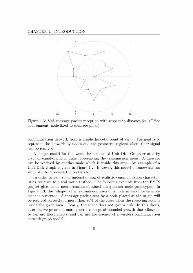
Figure 1.3: 80% message packet reception with respect to distance [m] (Officeenvironment, node fixed to concrete pillar).
communication network from a graph-theoretic point of view. The goal is torepresent the network by nodes and the geometric regions where their signalcan be received.
A simple model for this would be a so-called Unit Disk Graph created bya set of equal-diameter disks representing the transmission areas. A messagecan be received by another node which is inside this area. An example of aUnit Disk Graph is given in Figure 1.2. However, this model is somewhat toosimplistic to represent the real world.
In order to gain some understanding of realistic communication character-istics, we turn to a real world testbed. The following example from the EYESproject gives some measurements obtained using sensor node prototypes. InFigure 1.3, the “shape” of a transmission area of a node in an office environ-ment is presented. A message packet sent by a node placed at the origin willbe received correctly in more than 80% of the cases when the receiving node isinside the given area. Clearly, the shape does not give a disk. In this thesis,later on, we present a more general concept of bounded growth that allows usto capture these effects, and capture the essence of a wireless communicationnetwork graph model.
6

1.3. EFFICIENT NETWORK ORGANIZATION
Next to communication in wireless networks, interference during simultane-ous transmissions is also of great importance. This interference can be modeledby a conflict graph, and this graph has a similar structure as the wireless com-munication graph. When presenting the models for wireless communicationnetworks, we consider both ways to define such a network.
1.3 Efficient Network Organization
With respect to wireless communication networks, in the following, we are inter-ested in the problems concerning the creation of subsets of nodes in the network.
The approaches we are considering in this thesis are for the creation ofsubsets of the nodes with certain properties:
• Independence:
A subset of nodes is called independent if no two nodes in this subset areconnected.
• Domination:
A subset of nodes is called dominating if every node in the network iscontained in this subset, or is connected to a node in it.
Nodes in an independent set do not interfere each other during simultaneoustransmissions, and nodes in a dominating set can be used to efficiently reachthe entire network by broadcasts from only these nodes. Note that a subset ofnodes can satisfy both properties. Such a subset is called maximal independentset.
There are many different perspectives from which we may look at the men-tioned structures and their construction by an algorithm. Considering the cardi-nalities of the respective subsets, we obtain optimization problems. Looking atthe in-network creation of such subsets, it is already challenging to create thesesubsets by a locally executed algorithm in each node even when not consider-ing cardinality explicitely. In the following chapters, we discuss independentand dominating sets from various angles, and in relation to graphs that modelwireless communication networks.
Besides the above basic versions of the considered problems, there also existweighted versions: each node is given a weight, and the goal is then to finda structure of minimum or maximum weight. A weight may correspondent tothe capabilities of the nodes to perform additional duties. The weights can bedetermined taking into consideration aspects like residual energy of a node, its
7

CHAPTER 1. INTRODUCTION
memory and processing power, and local figures like number of neighbors ormobility indicators. Usually, these weights are locally computed in each node,and they depend on the application the resulting structure is created for.
Independent and dominating sets in wireless networks are used in a varietyof different applications, especially at the lower layers directly involved withcommunication strategies, and directly dealing with the topology of the com-munication network. Some of these applications are presented next.
• Clustering
Clustering is often used in large-scale networks to reduce the complexity.On a topology level, clustering is done by grouping nodes inside a certainarea, which are then controlled by a designated node called clusterhead.These clusterheads are chosen so that they satisfy both the independenceand domination property. This results in a well-distributed structure thatcovers the entire network.
For example, in [24], the use of independent set based clustering for theallocation of bandwidth and channels to support multimedia traffic is pro-posed. The question of cluster sizes, i.e. the number of nodes in eachcluster, and their fair distribution are addressed in [45].
• Routing and Flooding
In a dynamic multi-hop communication network, routing schemes thatadapt to the changing topology are required. Each individual node isneither able to store the entire topology information, nor to keep up-dated information about the changes in the network topology. There aremany on-demand routing algorithms designed for mobile ad-hoc networks.These algorithms create and sometimes maintain routes for data packetsto be sent via relay nodes through the network to reach a destination.When trying to establish a new route, that is, trying to find the desti-nation in the network together with a path leading there, these schemeshave to rely on flooding the network to do so. Examples of such ad-hocrouting schemes are Dynamic Source Routing (DSR, [31]) and Ad-Hoc On-Demand Distance Vector routing (AODV, [52]), and many improvementsbased on these schemes.
Basic, network-wide flooding causes the broadcast storm problem [43], re-sulting in excessive contention and collisions, i.e. a large communicationprotocol overhead. Using a dominating set of small size as a virtual back-bone to propagate flooding messages overcomes this problem, and greatly
8

1.4. CONTRIBUTIONS
reduces the number of messages needed, and thus the protocol overheadas well [2, 13, 55].
• Sleeping Patterns
Wireless sensor networks are expected to be in operation for a long periodof time, running on batteries. For example in event detection applications,there are long periods of inactivity, which allow the nodes to follow a sleep-state schedule where the radio hardware can be turned off for certain timeintervals to save energy. However, the network has to remain functional,and most importantly connected so that a detected event can successfullybe reported to the sink.
An example of a connected dominating set based solution that exploitsthe redundancy present in the network is presented in Chapter 6.
Also from a theoretical point of view, independent and dominating sets withrespect to graphs that model wireless communication networks are of outstand-ing interest. For example, in distributed computing, independent sets capturethe important notion of symmetry breaking in a simple statement. The theo-retical aspects of these structures are discussed, and introduced in detail in thefollowing Chapter 2.
1.4 Contributions
In this thesis, we look at independent and dominating sets in wireless com-munication networks, both from a theoretical background and from practicalimplementations.
For wireless ad-hoc and sensor networks, many graphical models are pro-posed in the literature to represent the communication links in such networks.We review these mostly geometrically defined models, and relate them to aunified structural property called bounded growth which is common in all ofthese models. Bounded growth is defined without geometric information, whichallows us to work with wireless communication networks based on adjacencyinformation only.
We consider the optimization problems of creating large independent sets,and small dominating sets in wireless communication graphs. These problemsare hard to solve to optimality, and we therefore consider approximative solu-tions. These are given by a polynomial-time approximation scheme (PTAS) that
9
CHAPTER 1. INTRODUCTION
creates a near-optimal solutions, that is, solutions with an error of (1+ε), ε > 0,in efficient run time.
The question whether there exists a PTAS for the Maximum Independent Setand Minimum Dominating Set problems in Unit Disk Graphs that work withoutexplicitely exploiting a geometric representation was an open problem. It wasexpressed since the first appearance of approximation schemes for these prob-lems on geometric graphs in [29] (1985). We eventually give a positive answerto this question by presenting an approach that yields a PTAS for graphs withthe polynomially bounded growth property, which includes Unit Disk Graphs.
Additionally, the approaches that give the approximation schemes for theseproblems can be extended towards robust algorithms in the sense that theyaccept any graph as input, and either return a (1 + ε)-approximate solution, ora certificate showing that the input graph does not satisfy the bounded growthproperty of a wireless communication graph.
Wireless ad-hoc networks lack central control. Locally executed algorithmsare thus of great importance. In the area of distributed computing, the problemof fast, i.e. poly-logarithmic time, local construction of maximal independentsets is a longstanding open problem. For the class of graphs with boundedgrowth, we present such a fast approach, again without relying on any geometricinformation. So, for bounded growth graphs, there is a positive answer to thisquestion, as well.
The presented local, distributed algorithm yields a PTAS for the above opti-mization problems. By extending the ideas behind the centrally executed PTAS,we obtain the first distributed approximation schemes for the Maximum Inde-pendent Set and Minimum Dominating Set problems on wireless communicationgraphs.
In addition to these contributions on the theoretical background of indepen-dent and dominating sets in wireless communication graphs, we also discuss apractical implementation of an efficient communication protocol for wireless sen-sor networks. We show that a cross-layer approach for communication in WSNsis a very efficient way to achieve the goal of long network lifetime running onbatteries.
1.5 Structure of the Thesis
In the first part of this thesis, in Chapters 2 – 5, we focus on the theoreticalbackground of wireless communication graphs, and algorithmic approaches bothfrom a global and local point of view.
10

1.5. STRUCTURE OF THE THESIS
In Chapter 2, the definitions of independent and dominating sets in networksare given together with basic properties of these structures. There, we focus onthe structures and resulting problems from a graph-theoretic point of view andpresent the general models for computation and communication in networks.In order to make statements about the efficiency of the approaches discussedin this thesis, we provide a theoretical base for algorithms running in eachwireless device (Section 2.1), and for communication patterns that allow thesedevices to collaborate by exchanging messages (Section 2.3). These modelsallow to abstract away from actual hardware and communication strategies,and therefore allow to give results that are independent of these. Chapter 2is—so to say—the second half of the introduction.
Wireless networks, created by the possible direct communication links be-tween the radios of several devices, result in specially structured graphs. Theseare presented in Chapter 3. Depending on the assumptions on the propagationof the radio waves being emitted by a wireless device, different graph modelsemerge, most of which are geometrically defined. However, all these modelshave a common structural property called bounded growth which is defined anddiscussed.
In Chapter 4, we consider the optimization problems of constructing inde-pendent sets of large size or weight, and dominating sets of small cardinality.For these optimization problems on wireless communication graphs, we presentpolynomial-time approximation schemes (PTASs) that are independent of geo-metric information. Robustness of the approaches is also discussed.
The focus in Chapter 5 is on local, distributed algorithms that are required inwireless ad-hoc networks. We present a fast, local approach for the constructionof a maximal independent set in graphs of bounded growth. This approach,together with the ideas of the preceding chapter, is extended towards distributedapproximation schemes that compute near-optimal independent and dominatingsets using local information exchange only.
Chapter 6 is concerned with an energy-efficient communication strategy forwireless sensor networks. There, we focus on a practical application of an in-dependent and dominating set. After shortly presenting the architecture ofa WSN, we present a cross-layer approach that locally schedules collision-freecommunication, and creates a backbone that is used for the communication inthe network. The approach is called EMACs (EYES Medium Access ControlScheme).
In Chapter 7, we conclude the thesis with a short summary of the key resultsand approaches.
11

CHAPTER 1. INTRODUCTION
12
Chapter 2
Definitions andPreliminaries
This chapter gives a detailed introduction into the problems consid-ered in this thesis, as well as a description of the underlying modelsof computation and communication. Basic definitions are presented,and an overview of complexity classes and optimization problems ingeneral is given.In wireless networks, in-network computation and communication iscrucial. In order to capture the characteristics of this paradigm, theLOCAL message passing model is introduced as a framework fordistributed algorithms in wireless, ad-hoc networks.The main structures of this thesis, independent and dominating setsin a graph, are defined in Section 2.2. Furthermore, basic properties,resulting problems and relations between these are discussed. Also,a simple greedy approach creating an independent and dominatingset is presented.
13

CHAPTER 2. DEFINITIONS AND PRELIMINARIES
This chapter provides the theoretical base of the thesis. We start by introducinga formal description of a “problem”, an algorithm to solve it, a notion of thequality of a solution to it, and a notion of time it takes an algorithm to computesuch a solution. In short, Section 2.1 sketches the basics of complexity theoryas required for the rest of this thesis.
In Section 2.2, we define the structural properties of independence and dom-ination for a subset of vertices in an undirected graph. The simple structureof a maximal independent set, which is both independent and dominating, isexplained. We also introduce and discuss the resulting optimization problems,i.e. computing a subset with such a property of largest or smallest cardinalitypossible. These problems are the Maximum Independent Set and MinimumDominating Set problem.
Large scale wireless communication networks like WSNs not only lack centralcontrol, but also each individual node lacks the capacity to store informationabout the entire topology of the network. In order to sufficiently describe andreason about algorithms which run locally in each node of such networks, weintroduce the LOCAL message passing model in Section 2.3. This model cap-tures these basic properties of wireless networking and in-network processing,while not being too concerned about the technical and hardware-specific detailsof communication.
In the last section of this chapter, a simple greedy strategy to create amaximal independent set, which is also a dominating set, is presented. Thisstrategy serves as an important example also used later in this thesis, and wegive both a centralized and local, distributed version of it.
2.1 Complexity and Approximability
In this section, we give some basic notions of problems, their complexity, andalgorithms to solve them. A more complete overview can be found in [23]. Inorder to do optimization, and to analyze algorithms and complexity, we need todefine the essence of optimization: a problem.
Definition 2.1. A problem is given by a problem description Π, which is apair (I,S) such that
• I denotes the set of instances of Π, and
• for each x ∈ I, S(x) is the set of feasible solutions.
14

2.1. COMPLEXITY AND APPROXIMABILITY
We consider two types of problems called decision and optimization prob-lems, which are given by refining the above general problem description.
Definition 2.2. Let Π be a problem description whose set I of instances ispartitioned into two sets Y and N = I \Y, called positive and negative instancesas follows:
x ∈ Y ⇐⇒ S(x) 6= ∅.
Seeking an answer to the question of whether an instance x ∈ I belongs to Y iscalled a decision problem.
The aim of a decision problem is to recognize the positive instances, that is,those instances that have a feasible solution.
For optimization problems, we look at problem descriptions, where addition-ally each feasible solution is evaluated by an objective function as follows. For aninstance x ∈ I together with a feasible solution y ∈ S(x), there is an objectivefunction value (or measure) f(x, y) ∈ N of that solution.
For each instance, the objective function may take on different values fordifferent feasible solutions. We are interested in solutions which minimize ormaximize this value with respect to all feasible solutions for such an instance.
Definition 2.3. In a problem description Π, for each pair of instance x ∈ Iand feasible solution y ∈ S(x), let the objective function f(x, y) assign a positiveinteger to this pair. The problem Πmin:
Given an instance x ∈ I, find a solution y∗ ∈ S(x) such that for everyy ∈ S(x),
f(x, y∗) ≤ f(x, y)
holds.
is called a minimization problem, and y∗ is called an optimal solution forthis problem.
Analogously, a maximization problem is defined by finding a solution withmaximum objective value over all feasible solutions. The question of minimiza-tion or maximization for an optimization problem is called goal of the problem.Note that in the above definition, the range of an objective function f can easilybe relaxed to rational numbers.
It is easy to see that any optimization problem Π can be transformed in astraightforward way into a corresponding decision problem. This is done by look-ing at the following, modified set of feasible solutions in case of minimization.
15

CHAPTER 2. DEFINITIONS AND PRELIMINARIES
Given an instance x ∈ I and a rational number τ , let
Sτ (x) := y ∈ S(x) | f(x, y) ≤ τ
denote the set of feasible solutions for the corresponding decision problem.Clearly, for an instance x, the decision problem based on Sτ (x) is equivalentto the following problem statement
Given an instance x ∈ I and a rational number τ , is there a solutiony ∈ S(x) so that f(x, y) ≤ τ ?
The maximization case is obtained in a symmetric way.For all the above problems, we can describe strategies and approaches which
generate answers to the problems by algorithms. Generally speaking, an algo-rithm A for a problem Π is a finite sequence of instructions or calculations tobe performed whenever an instance x ∈ I is presented to A, and that returnssome solution from S(x) when all these instructions have been performed. Thesolution returned is referred to as output of A for the instance, or A(x). For op-timization problems, an output is usually considered together with its objectivevalue f(x,A(x)).
The instance x ∈ I is also called input, especially when considered in relationwith an algorithm for the problem at hand, and the value given by the objectivefunction f(x, y) for a solution y ∈ S(x) is usually called cost.
For a problem Π, we define the length |x| of an instance x ∈ I as the numberof bits used to specify x in some fixed encoding. The time-complexity, i.e. thenumber of elementary steps it takes for an algorithm to return a solution, ismeasured as a function of the length of an input instance. The computationtime, or run time, of an algorithm is measured by the number of basic opera-tions it performs, e.g. additions, comparisons, multiplications etc. We supposethat all algorithms run on the same machine model, the random access ma-chine (RAM), which is polynomially related to the Turing machine and otherreasonable computational models.
The run time is usually expressed in asymptotic notation. For two functionsf : N → R+ and g : N → R+, we say that “f is in the order of g”, writtenf(n) = O(g(n)) for short, if there exist c, n0 ∈ N such that f(n) ≤ c · g(n) forall n ≥ n0. While this O-notation gives an upper bound, we can analogouslydefine f(n) = Ω(g(n)) for lower bounds to say that “f is at least in the orderof g”. It is f(n) = Ω(g(n)) ⇐⇒ g(n) = O(f(n)).
If the run time of an algorithm A is bounded by a polynomial p(|x|) for allpossible instances x ∈ I, thus, for any instance x and some fixed k ∈ N, A is an
16

2.1. COMPLEXITY AND APPROXIMABILITY
algorithm with run time O(|x|k), then we say that A is efficient. A problem thatcan be solved by an efficient algorithm is referred to as polynomially solvable.
A problem that can be solved in polynomial time is generally consideredeasy. However, in the next chapters, we concentrate on problems which arehard. The notion of hard problems is formalized based on decision problems.The resulting complexity hierarchy of problems has been extended ever sincethe first appearance of the class NP together with NP-complete problems in the1970s [11].
2.1.1 Decision Problems and the Class NP
The class NP consists of all decision problems that can be certified in poly-nomial-time: That is, a decision problem is in NP if there is a (necessarilypolynomial size) “certificate” which shows that an input instance is a positiveinstance, and that there is a polynomial time algorithm which can verify thiscertificate with respect to the problem.
The class P consists of all those decision problems that can be recognizedin polynomial time, i.e. for which the decision of an instance to be a positiveinstance can be reached in polynomial time.
Clearly, P ⊆ NP holds. However, the question whether P = NP or P 6= NPis open. It is widely believed that P 6= NP, and a good reason for this is givenby the class of NP-complete problems. The class of NP-complete problems hasthe following compelling property: if one can prove that a single NP-completeproblem actually is in P, then P = NP. The reason for this comes from the factthat all NP-complete problems are polynomially reducible to each other.
Let Π1,Π2 ∈ NP. The problem Π1 is polynomially reducible to Π2 if thereexists a polynomial time algorithm that for every instance x1 of Π1 producesan instance x2 of Π2 so that x1 is a positive instance of Π1 if and only if x2 isa positive instance of Π2.
Practically, this means that we can use an efficient algorithm for Π2 to solveΠ1 efficiently: simply transform the instance of Π1 into the respective instanceof Π2, and then solve this instance.
With the introduction of a polynomial reduction, we can formally introduceNP-complete problems [23].
Definition 2.4. A decision problem Π is NP-complete if
• Π is in NP, and
• all other NP problems are polynomially reducible to Π.
17

CHAPTER 2. DEFINITIONS AND PRELIMINARIES
Polynomial reduction is a transitive relation on the class NP. If a problemΠ1 is polynomially reducible to Π2 and Π2 is reducible to Π3, then Π1 is alsoreducible to Π3. This fact can be exploited to show that a new problem Πis NP-complete since it now suffices to show that Π is in NP and that thereis an NP-complete problem which is polynomially reducible to Π. The start,i.e. the first problem shown to be NP-complete, was made by the satisfiabilityproblem (SAT) [11], and today there are numerous problems that are known tobe NP-complete.
2.1.2 NP-Optimization Problems
Similar to the class NP for decision problems, we introduce the class NPO foroptimization problems [12]. For this class, we consider optimization problemsfor which the length of feasible solutions is polynomially bounded in terms ofthe length of an instance, and for which the value of the objective function canalso be computed in polynomial time. More formally, an optimization problemΠ is in the class NPO if
• all solutions are short, that is for every x ∈ I, and every y ∈ S(x), wehave |y| ≤ p(|x|) for some polynomial p,
• for any x and any y with |y| ≤ p(|x|), the question whether y ∈ S(x) canbe decided in polynomial time, and
• given x ∈ I and y ∈ S(x), the objective function f(x, y) is computable inpolynomial time.
The class PO then corresponds to all optimization problems in NPO that canbe solved to optimality in polynomial time. Again, we are interested in the hardproblems, given by the following definition.
Definition 2.5. A problem Π is said to be NP-hard if every problem in NPcan be solved in polynomial time using a polynomial time algorithm that solvesΠ as a subroutine.
Note that in the above definition, we no longer restrict Π to be a decisionproblem. In particular, this definition includes all optimization problems forwhich the corresponding decision problem is NP-complete. Furthermore, it iseasy to see that if P 6= NP holds, then PO 6= NPO has to hold, as well.
In order to show that a problem Π is NP-hard, it suffices to show that anNP-complete problem Π′ could be solved efficiently by efficiently solving Π. Allother problems in NP are polynomially reducible to Π′.
18

2.1. COMPLEXITY AND APPROXIMABILITY
From an algorithmic point of view, knowing that an NPO problem is NP-hard, we also know that we cannot compute an optimal solution in polynomialtime, unless P = NP. In this case, there are two major options.
• On the one hand, we can abandon the idea of polynomial time, and stillrequire an optimal solution from an algorithm. One way to achieve thiswould be complete enumeration, which may lead to exponential run time,in the worst case with an exponent only bounded by the polynomial boundon the size of all solutions.
• On the other hand, we can sacrifice optimality and start looking for ap-proximate solutions which are computed by a polynomial time, i.e. effi-cient, algorithm.
The latter approach is taken in this thesis.Let Π be an NPO problem. For any instance x ∈ I, denote by s∗(x) the cost
of an optimal solution. The performance ratio of any feasible solution y ∈ S(x)is then given by
R(x, y) := max
f(x, y)
s∗(x),
s∗(x)
f(x, y)
.
Note that the performance ratio is always greater than or equal to 1, inde-pendent of the goal: the first fraction is used for minimization, the second formaximization problems. Clearly, the closer R(x, y) is to 1, the closer a solutionis to an optimal solution. The performance ratio is also called approximationratio.
Definition 2.6. Let Π be an NPO problem, and let A be an algorithm that, forevery instance x ∈ I, returns a feasible solution A(x) ∈ S(x). Given a functionr : N → [1,∞), the algorithm A is an r(n)-approximate algorithm if forevery instance x ∈ I, the inequality
R(x,A(x)) ≤ r(|x|)
holds. If there exists an r(n)-approximate polynomial time algorithm for Π, wesay that Π is approximable within r(n) (in polynomial time).
An algorithm which actually gives a constant performance ratio independentof the length of the instance is referred to as constant-factor approximation. AnNPO problem Π belongs to the class APX if it is approximable within α (inpolynomial time), for some constant α > 1.
19

CHAPTER 2. DEFINITIONS AND PRELIMINARIES
NPO
POPTAS
APX
Figure 2.1: Relationships between some complexity classes for optimizationproblems discussed in this thesis.
Definition 2.7. A family Aεε>0 of (1+ε)-approximation algorithms is calledan approximation scheme.
If, for each fixed ε > 0, the (1 + ε)-approximation algorithm Aε of an ap-proximation scheme Aεε>0 runs in polynomial time in the input size, we callAεε>0 a Polynomial-Time Approximation Scheme (PTAS).
An NPO problem that admits a PTAS is also in the class PTAS. We onlydemand the run time of a PTAS to be polynomial in the size of the inputinstance, and not in the desired performance ratio parameter 1/ε. Computationtimes of 21/ε ·p(|x|) or O(|x|1/ε) are allowed, obviously resulting in high run timewhen ε is close to 0.
Figure 2.1 gives the relations between the complexity classes for NPO prob-lems [54]. It is easy to see that the inclusions given are strict if and only ifP 6= NP. Especially to stress the difference between the classes APX and PTAS,there is also the notion of APX-complete problems. APX-complete problems arethose problems in NPO that are the most difficult ones to approximate. Looselyspeaking, an NPO problem is APX-complete if there exists a bound α > 1 suchthat there exists no polynomial time α-approximation for this problem unlessP = NP. Thus, if P 6= NP, for APX-complete problems, there cannot exist apolynomial-time approximation scheme.
There is a long list of other complexity classes and notions, in fact, a whole“complexity zoo” [14]. Here, we only presented the major classes that are ofimportance for this thesis. For a rigorous introduction to the theory of NP, we
20

2.2. STRUCTURES AND OPTIMIZATION ON GRAPHS
refer the reader to the classic book by Garey and Johnson [23]. A list of NPO-complete problems from various application areas is given by [12], includingmany further references.
2.2 Structures and Optimization on Graphs
In this section, we define several graph-theoretic structures, which are frequentlyused in efficient communication strategies for wireless networks, and the result-ing optimization problems. These structures are independent and dominatingsets of vertices in a graph. Before the respective definitions, we first introducesome notation which is used commonly throughout this thesis.
Communication networks are modeled as undirected graphs G = (V,E).Here, the vertices V represent the communication devices or nodes, and twonodes are connected by an edge in E ⊆ V ×V if they can communicate directlywith one another. We set n := |V |, and denote by ∆ the largest degree ofa vertex in G. Furthermore, we assume the set of vertices to be ordered, forinstance and simplicity V = 1, . . . , n. In this thesis, we are interested inalgorithms that identify and create subsets of the vertices which satisfy certainstructural properties. Also, as soon as we consider the cardinality or weight ofsuch a subset as a measure for the quality of a solution, optimization problemsarise.
Let V ′ ⊆ V be a subset of vertices in G = (V,E). In the following, we useG[V ′] to denote the subgraph induced by V ′. For a subgraph G′ of G, we useV (G′) and E(G′) to refer to the vertices and edges of G′ respectively.
In case of a weighted graph, that is, each vertex v ∈ V is additionally givena weight wv, we define the weight of a subset V ′ ⊆ V by W (V ′) :=
∑
v∈V ′ wv.
For a subset V ′ ⊆ V , let maxV ′ be the vertex u ∈ V ′ with highest number,or weight in a weighted graph. In the latter case, we use the highest number tobreak a possible tie when vertices have the same weight.
Furthermore, we denote by Γ(v) the closed neighborhood of a vertex v ∈ V ,i.e.
Γ(v) := u ∈ V | (u, v) ∈ E ∪ v.
Analogously, for V ′ ⊆ V , let Γ(V ′) :=⋃
w∈V ′ Γ(w) define the neighborhood ofV ′. In this context, we set Γ(∅) := ∅. For r ∈ N, we call Γr(v) := Γ(Γr−1(v))the recursively defined r-th neighborhood of v ∈ V , where Γ0(v) := v. Us-ing the graph-theoretic distance dG(u, v), denoting the number of edges on ashortest path in G between vertices u and v, we can equivalently define the r-th
21

CHAPTER 2. DEFINITIONS AND PRELIMINARIES
neighborhood of v as
Γr(v) := u ∈ V | dG(u, v) ≤ r.
2.2.1 Independent Sets
Two vertices of a graph G = (V,E) are called independent if they are notadjacent to one another. As a consequence, the subgraph G[I] induced by anindependent set I contains no edges.
Definition 2.8. A subset I ⊆ V is called independent if for every two verticesu, v ∈ I, there does not exist an edge (u, v) ∈ E.
An independent set is called maximal if it cannot be extended by the addi-tion of any other vertices from the graph. Note that maximality of an indepen-dent set is a purely structural property; we do not require such a set to be oflarge cardinality. A maximal independent set in G is further on abbreviated byMIS. For any graph, a MIS can easily be generated by a greedy approach. InSection 2.4, we will explain such an approach as an example.
When looking at the cardinality of an independent set, we obtain an opti-mization problem. The Maximum Independent Set (Max-IS) problem tries tofind an independent set of maximum cardinality. Clearly, a maximum indepen-dent set is also maximal, but not vice versa.
In general, in an undirected graph, computing a Maximum Independent Setis NP-hard. Even more, it cannot be efficiently approximated within n1−ε (un-less P = NP, [27]). There exists a polynomial time O(n/ log2 n)-approximationusing subgraph-removal techniques (see [7]).
2.2.2 Dominating Sets
A broadcast from a communication node is received by all its neighbors. Thisis captured in the notion of domination in a graph G = (V,E).
Definition 2.9. A subset D ⊆ V of vertices is called dominating if everyvertex in V is contained in the subset, or adjacent to a vertex in this set D.
A dominating set can also be used for subsets of vertices V ′ ⊆ V , such a setD′ then dominates V ′ if V ′ ⊆ Γ(D′) holds. There is an important relationshipbetween maximal independent sets and dominating sets in a graph. Throughoutthis thesis, we will often rely on the following theorem.
22

2.2. STRUCTURES AND OPTIMIZATION ON GRAPHS
Theorem 2.10. Given a graph G = (V,E), any maximal independent set I ⊆ Vis also a dominating set.
Proof. Suppose there exists a non-dominated vertex in V \ I. This vertex couldbe added to I while keeping the independence property, thus violating maxi-mality.
The Minimum Dominating Set (Min-DS) problem asks for a dominating setof minimum cardinality. The problem is NP-hard on undirected graphs, and forefficient approximations, there is a lower bound of (1− ε) ln n, for ε > 0, on theapproximation ratio (unless every NP problem is solvable in time nO(log log n),[21]).
There are also further variants of dominating sets in a graph G = (V,E) bydemanding additional properties for a dominating set D ⊆ V :
• Minimum Connected Dominating Set (Min-CDS)If D consists of a single connected component, it is referred to as ConnectedDominating Set. Of course, if G is not connected, such a structure doesnot exist.
• Minimum Independent Dominating Set (Min-IDS)If we want to find a small subset of vertices that is both dominating andindependent, we call the resulting problem Minimum Independent Domi-nating Set problem. In light of Theorem 2.10, this problem is sometimesalso called Minimum Maximal Independent Set problem. Note that theMaximum Independent Dominating Set problem is equivalent to findinga Maximum Independent Set.
As with the Min-DS problem, the Min-CDS problem cannot be efficientlyapproximated within (1 − ε) ln n, ε > 0, unless every problem in NP can bedeterministically solved in time nO(log log n). The Min-IDS problem cannot beefficiently approximated within a factor of n1−ε for any ε > 0 (unless P = NP,[26]).
The problems presented can be extended to vertex-weighted problems. Whilethe constraints for the feasibility of a solution remain the same, the objectivefunction is altered to include the weights of the vertices instead of the cardinalityof the subsets. Further on, unless stated otherwise, we consider the unweightedversions of the problem.
23

CHAPTER 2. DEFINITIONS AND PRELIMINARIES
2.3 Distributed and Local Algorithms
In this thesis, we are interested in efficient algorithms that create independentand dominating sets, both from the structural, e.g. maximal sets, and theoptimization, e.g. maximum cardinality sets, point of view. Also, due to thewireless structure and resource-poor nature of the underlying communicationnetwork, we are interested in algorithms that account for this fact. We now goon to present a model for the local communication characteristics of wirelessnetworks which we use to describe locally executed algorithms.
A prominent characteristic of wireless ad-hoc networks is the lack of cen-tral control. Even if a central base station is present in the communicationnetwork, the resulting communication and coordination overhead may be pro-hibitive to centrally organize and optimize such a network. In this part, weprovide a framework, or model, for distributed and local computing that allowsfor capturing the effects of communication and coordination overhead, as wellas the non-centralized nature of wireless networks: the LOCAL message passingmodel [40, 51].
Consider a simple, undirected graph G = (V,E) which represents the point-to-point communication network. That is, the vertices are the (wireless) nodes,and two nodes are connected if and only if they can communicate with oneanother directly. Note that we only consider bidirectional communication, e.g.by ignoring unidirectional links.
For this communication network, we would like to point out that the graph isused two-fold: it represents both the communication network and the graph forwhich we seek solution subsets. In other words, G is the graph we work in andoptimize for. This also follows from the application, as independent and dom-inating sets in communication networks are used for efficient communicationstrategies in the network itself.
A vertex in the graph has—possibly among others—two main parts we focuson: a processing part including CPU and memory, and a communication partwhich allows the vertex to send messages to its direct neighbors in G. Weassume that each vertex v ∈ V is given a unique identifier idv at the hardwarelevel. For concreteness and simplicity, we assume these identifiers to be ordered,i.e. idv ∈ N for every v ∈ V , and furthermore, that each identifier is stored inthe node using O(log n) bits. Usually, the explicit distinction between a vertexv and its identifier idv is neglected, we simultaneously use v to denote both.
We now explain the communication characteristics of the LOCAL model.The networking on G operates in so-called global communication rounds. Ba-sically, in one round, each vertex is able to communicate once with each of its
24

2.3. DISTRIBUTED AND LOCAL ALGORITHMS
neighbors by transmission of a message packet, and perform some computation.To be more precise, a round is divided into two parts. First, a vertex can per-form some computations, and then communicate with its neighbors in G bysending and receiving message packets. In one round, a vertex can send at mostone message to, and receive at most one message from each individual neigh-boring vertex. The order in which messages are sent and received in a round bythe individual vertices is not specified, and assumed to occur simultaneously. Avertex that wants to reply to a message received from a neighbor can only doso in succeeding rounds.
As a consequence of this local, round-based communication pattern, for twovertices u, v ∈ V with d(u, v) = k, it takes at least k rounds for a message sent byu to reach v via message forwarding of intermediate vertices. This also impliesthat a vertex, in a constant number of rounds, can only obtain informationabout the topology of its local neighborhood of constant radius.
We assume communication in the network to be synchronized, that is, in theLOCAL model, each vertex has the same notion of a round. The round-basedsynchronization is not to be confused with synchronization of time, a much moredifficult task in distributed systems. In the LOCAL model, we only require thevertices to be in the same round during the execution of a distributed algorithm.This limitation is, however, not too severe. At the cost of higher messagecomplexity, with the introduction of synchronizers [4], algorithms presented forthe synchronous model can be employed in asynchronous settings, as well.
While the complexity of the computations performed locally at each vertex(within one round) can be explained using the notions described in Section 2.1,the LOCAL model mainly captures the communication part. In order to quan-tify this part, there are three complexity measures for local algorithms in thisdistributed model:
• The distributed time complexity of a local algorithm is the number ofrounds until all vertices have terminated the algorithm.
Typically, in such synchronous systems, all vertices wake up simultane-ously, or start an algorithm at the same time. If we assume that a vertexstarts the algorithm upon receiving the first message that belongs to thedistributed algorithm at hand, we obtain an almost equivalent model. Inthis case, the time complexity is defined as the maximal time between thefirst vertex wake-up and overall termination.
• The number of messages sent during the execution is given by the messagecomplexity of the algorithm, and it is usually given with respect to a single
25

CHAPTER 2. DEFINITIONS AND PRELIMINARIES
vertex of the network.
• Each message packet used by the algorithm transports information to itsrecipient. The amount of information contained in a message packet, thatis, the length of such a packet, is called message size. The largest messageneeded to execute a local algorithm defines the maximum message size.In combination with the message complexity, this figure gives the overallexchanged amount of information in the network.
Up to now, in the LOCAL model, we allow that each vertex can address eachneighbor directly by a distinct message in each round. Especially in wirelessnetwork settings, this is not very realistic. Sending a message in such networksis usually done by a broadcast which can be received by all adjacent vertices.In the following, in order to explicitely stress this broadcast version of the localmodel, we denote it by LOCALBC.
In applications, the size of message packets is limited, and thus this factshould be taken into account. The latter is especially interesting in the broad-cast model, as a limited packet size may not allow distinct information for allneighboring vertices, e.g. when the neighborhood is larger than the packet size.When not considering the message size, and thus allowing message packets ofarbitrary length, the LOCAL and LOCALBC models are clearly equivalent: inthis case, all messages to distinct neighboring vertices are combined into onelarger message. This larger message is then broadcast in the respective round,and each neighboring vertex filters out the part concerning itself.
In the following, we assume that the message size is at least Ω(log n), other-wise a vertex cannot even inform its neighbors about its identifier, and adjacentvertices would become almost indistinguishable, giving an anonymous network.We also suppose that each node has knowledge of the identifiers given to itsneighbors. This can easily be achieved by a single broadcast of each node con-taining its identifier at the beginning of operation.
The synchronous, local message passing model seems to be a reasonableabstraction for communication-based algorithms in wireless ad-hoc networks,both from a theoretical and practical point of view.
• For the theory of local, distributed computing, it is the simplest model todescribe algorithms for, and to reason about. Also, the focus is put onlyon the additional overhead that stems from locality and communication,independent of characteristics thereof.
• In practice, round-based communication can easily be achieved or is ex-plicitely done. For example, TDMA-based medium access control imme-
26

2.3. DISTRIBUTED AND LOCAL ALGORITHMS
diately maps to the synchronous message passing model. This can be seenin Chapter 6 when dealing with the EMACs protocol.Also, in contrast to communication, computation is cheap in wireless com-munication, both with respect to time and energy consumption.
The main questions in local computing deal with the relation between a so-lution composed of local, partial solutions with respect to an optimal (global)solution for optimization, and how to compute these by local, distributed algo-rithms. The characteristics of the LOCAL model, the lack of central control andglobal information, limit the possibilities in computing. In this model, alreadythe fast creation of a structure like a maximal independent set is a non-trivialtask.
In this context, maximal independent sets play an important role since thecreation of this structure captures the notion of symmetry breaking in a simpleproblem formulation. Being this prototypical, fast MIS creation has receivedparticular attention in the literature.
The fastest known deterministic distributed algorithm is based on the notionof network decompositions introduced in [5], and is given in [50]. The authors
obtain a deterministic O(n(√
1/ log n)d
) algorithm, where d is a constant.
Furthermore, there is also an elegant randomized algorithm for MIS creationwith expected time complexity of O(log n) presented in [39].
An important function, which is used quite often in the area of local algo-rithms is the “logstar”-function. This function is defined as
log∗n := mini ∈ N | log log . . . log︸ ︷︷ ︸
i
n ≤ c
for some constant c.
A lower bound of Ω(log∗n) for the distributed computation of maximal in-dependent sets is given in [38]. This lower bound states that even on a ring Cn,at least time Ω(log∗n) is required to construct a MIS.
For general graphs of bounded maximal degree ∆, a maximal independentset I can be computed locally in O(log∗n) communication rounds using messagesof size O(log n) [38, 51]. Thus, in case ∆ is bounded by a constant, there existsan asymptotically time optimal approach.
However, a deterministic, poly-logarithmic time distributed algorithm forMIS construction is a longstanding open problem.
27
CHAPTER 2. DEFINITIONS AND PRELIMINARIES
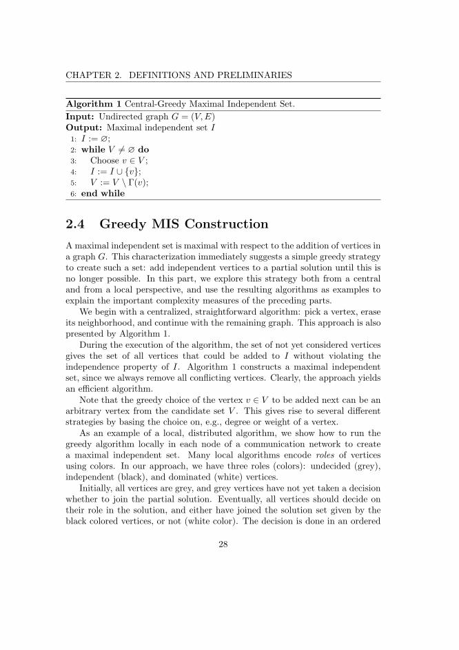
Algorithm 1 Central-Greedy Maximal Independent Set.
Input: Undirected graph G = (V,E)Output: Maximal independent set I1: I := ∅;2: while V 6= ∅ do3: Choose v ∈ V ;4: I := I ∪ v;5: V := V \ Γ(v);6: end while
2.4 Greedy MIS Construction
A maximal independent set is maximal with respect to the addition of vertices ina graph G. This characterization immediately suggests a simple greedy strategyto create such a set: add independent vertices to a partial solution until this isno longer possible. In this part, we explore this strategy both from a centraland from a local perspective, and use the resulting algorithms as examples toexplain the important complexity measures of the preceding parts.
We begin with a centralized, straightforward algorithm: pick a vertex, eraseits neighborhood, and continue with the remaining graph. This approach is alsopresented by Algorithm 1.
During the execution of the algorithm, the set of not yet considered verticesgives the set of all vertices that could be added to I without violating theindependence property of I. Algorithm 1 constructs a maximal independentset, since we always remove all conflicting vertices. Clearly, the approach yieldsan efficient algorithm.
Note that the greedy choice of the vertex v ∈ V to be added next can be anarbitrary vertex from the candidate set V . This gives rise to several differentstrategies by basing the choice on, e.g., degree or weight of a vertex.
As an example of a local, distributed algorithm, we show how to run thegreedy algorithm locally in each node of a communication network to createa maximal independent set. Many local algorithms encode roles of verticesusing colors. In our approach, we have three roles (colors): undecided (grey),independent (black), and dominated (white) vertices.
Initially, all vertices are grey, and grey vertices have not yet taken a decisionwhether to join the partial solution. Eventually, all vertices should decide ontheir role in the solution, and either have joined the solution set given by theblack colored vertices, or not (white color). The decision is done in an ordered
28

2.4. GREEDY MIS CONSTRUCTION
Algorithm 2 Local-Greedy Maximal Independent Set (code for vertex v).
Input: Undirected graph G = (V,E)Output: Maximal independent set v ∈ V | c(v) = black.1: c(v) := grey;2: while c(v) = grey do3: if ∃u ∈ Γ(v) | c(u) = black then4: c(v) := white;5: else if v = maxu ∈ Γ(v) | c(u) = grey then6: c(v) := black;7: end if8: end while
fashion, vertices with higher identifiers are allowed to decide first. A vertexwaits with its decision until all vertices with higher identifier have decided.
The algorithm works as follows: every grey vertex joins the partial solution(black vertices) when it has the highest identifier among its grey neighbors andif none of its neighbors has already joined. Vertices adjacent to a black verteximmediately turn white. A change of color always results in a local broadcastthat informs all neighbors about the new color. The local algorithm describingthe decision process is also given by Algorithm 2.
Clearly, the algorithm terminates, as the grey vertex with highest identifieralways changes its color and each black or white vertex never changes its coloragain. In order to obtain a MIS, after completion of the algorithm, the set ofblack vertices should be independent, and each white vertex should be neighborto at least one black vertex.
Lemma 2.11. The set of black vertices, as created by Algorithm 2, is a MIS
on G.
Proof. For the sake of contradiction, assume that there are two adjacent blackvertices, say u and v. W.l.o.g. let u < v, then at the same time as v decided toturn black, u could not have taken this decision due to line 5 not holding for u.After this decision, u has to change its color to white due to line 3.
To see that the solution is maximal, observe that as long as there are non-dominated vertices (grey), there is also a vertex with the highest identifier amongthese which will turn to black. White vertices are adjacent to a black vertex.
Let us now look at the complexity of this approach in the LOCAL messagepassing model. One round is given by a single execution of the while loop. In
29

CHAPTER 2. DEFINITIONS AND PRELIMINARIES
each round, at least the grey vertex with highest identifier changes its color andthus sends a message in this round.
There are exactly n color changes, therefore after at most Ω(n) communi-cation rounds, there are no grey vertices left and the algorithm has thus termi-nated. However, in each round, more than just a single vertex or few verticesmay change its color, possibly resulting in a faster distributed time complexity.
Unfortunately, for example by considering vertices along a line with increas-ing identifiers, there may actually be only a single point of activity duringthe execution, resulting in sequential time complexity of O(n) communicationrounds.
The message complexity (per vertex) is constant as a vertex only changesits color once, and therefore only has to broadcast this information once to allneighbors, which takes a single round.
A message containing information about a new color of the sender is ofconstant size. However, the algorithm assumes knowledge of the vertices’ iden-tifiers which requires messages of size Ω(log n). All messages are broadcasts,the algorithm therefore is also suited without change for the LOCALBC model.
30

Chapter 3
Wireless CommunicationGraphs
Wireless networks are created by the communication links between acollection of radio transceivers. The nature of wireless transmissionsdoes not lead to an arbitrary, undirected graph, but to a structuredgraph which we discuss in this chapter. We introduce geometri-cally inspired graph models which are commonly used to representwireless ad-hoc networks. All of these models share the property of(polynomially) bounded growth. This important property, which nolonger depends on the geometry, is defined and discussed.Bounded growth already allows for a constant bound on the approx-imation ratio of a solution given by a maximal independent set forthe Max-IS and Min-DS problems. Such a solution can easily becreated by the greedy strategies of the previous chapter.Implications of the geometry behind the wireless graph models, forexample recognition and geometric construction issues, are pointedout here. In this context, robust algorithms are also introduced.
31

CHAPTER 3. WIRELESS COMMUNICATION GRAPHS
A wireless, ad-hoc network is created by the communication links between acollection of radio transceivers. The nature of wireless transmissions does notlead to an arbitrary, undirected graph, but to a structured graph. This structure,called bounded growth, is introduced and discussed in this chapter.
We propose several geometrically inspired graph models for wireless commu-nication graphs. These range from very simple Disk Graphs to more realisticBounded Coverage Area Graphs, and most of these models are geometricallydefined [46]. They follow the general intuition that vertices which are close toone another can communicate directly, while far separated ones cannot reacheach other.
The bounded growth property of these models can be exploited to obtain ef-ficient optimization strategies: Maximal independent sets are already constant-factor approximations to the Max-IS and Min-DS problems. In terms of en-coding of the graphs, i.e. how the graph is presented as input to the algorithms,there are several possibilities. These go from giving the adjacency of each ver-tex to describing the geometric shapes and positions of the vertices, and bythen looking at the intersection graph of the geometric objects. The latter iscalled geometric representation, and in practice requires a localization schemethat gives each wireless node its position. We will discuss the implications andadvantages of these different input encodings.
In Section 3.1, we define bounded growth graphs. After that, we introduceprominent graph models that are used to model the communication in wire-less ad-hoc and sensor networks, and give their relation to bounded growth. InSection 3.3, a constant-factor ratio for the cardinality between a maximal in-dependent set and Maximum Independent and Minimum Dominating Sets areestablished for these particular graph classes. Before concluding this chapter,different representations of a graph, and various issues arising from these arediscussed. Robust algorithms, which are described in Section 3.5, are a possibil-ity to work around some problems with different representations of structuredgraphs.
3.1 Bounded Growth Graphs
Throughout this thesis, we are mostly interested in graph classes that modelwireless communication networks. However, characteristics of such networkshighly depend on the environment in which they operate, and we would like toabstract away from this environment. The smallest common structure of mostwireless graph models is bounded growth as given by the following definition.
32

3.2. GEOMETRIC INTERSECTION GRAPH MODELS
Definition 3.1. Let G = (V,E) be a graph. If there exists a function f(.) suchthat every r-neighborhood in G contains at most f(r) independent vertices, thenG is f-growth-bounded. In this case, we call f the growth function.
Furthermore, we say that G has polynomially bounded growth if for someconstant c ≥ 1, f(r) = O(rc) is bounded by a polynomial of maximal degree c.
Graphs of bounded growth are sometimes also called graphs of bounded(local) independence. Note that the growth function f(.) only depends on theradius of the neighborhood, and not on the number of vertices in G. Thus,for constant r, the number of independent vertices in Γr(v) is bounded by aconstant for any v ∈ V .
Especially when considering subsets of vertices, like independent or domi-nating sets, the following lemma shows that the bounded growth property of agraph is closed under taking induced subgraphs.
Lemma 3.2. Let G = (V,E) be an f-bounded growth graph. Then, for anyV ′ ⊂ V , the induced subgraph G[V ′] is also of f-bounded growth.
Proof. We prove the claim by contradiction. Suppose that there is a subsetV ′ ⊂ V such that the bound on the growth is violated for V ′. That is, for somer ∈ N, there exists a vertex u ∈ V ′, and a neighborhood Γr(u) in G[V ′] suchthat there is an independent set I ⊂ Γr(u) with cardinality |I| > f(r).
Consider the addition of any v ∈ V \V ′ to V ′, and and the resulting inducedgraph G[V ′ ∪ v]. It is easy to see that the independence property of I is stillsatisfied in G[V ′ ∪ v].
Furthermore, for every u′ ∈ Γr(u), it is dG(u, u′) ≤ dG[V ′](u, u′) ≤ r.Therefore, I is also an independent set with |I| > f(r) in the r-th neighbor-
hood of u when considering the original graph G.
It is easy to see that an f -bounded-growth graph does not contain a vertex-induced subgraph isomorphic to a K1,f(1)+1. Such a subgraph would immedi-ately violate the growth function f .
3.2 Geometric Intersection Graph Models
In the following, we propose several geometrically defined graph models thatrepresent wireless networks in various degrees of granularity with respect toreality. We also apply and check Definition 3.1 on the geometric graphs toestablish bounded growth for these models.
33

CHAPTER 3. WIRELESS COMMUNICATION GRAPHS
A wireless ad-hoc network is created by nodes that are equipped with atransceiver, and that are placed in the real world. The environment, especiallythe positions of the nodes, has to be accounted for, and it does not surprise thatmost wireless graph models are therefore defined for the Euclidean space. Inthe following, we use ‖.‖ to denote the Euclidean distance in R
2.Usually, the models result from geometric intersection or containment graphs
which give the general idea behind these models. Next, we therefore introducethese graph models in general, and then specify additional characteristics inorder to justify them for the purpose of modeling wireless communication net-works.
We assume that the vertices of the graph, i.e. in our case the wireless nodes,are placed in the 2-dimensional Euclidean plane. In other words, there existsa mapping p : V → R
2 which gives each vertex v ∈ V its location pv ∈ R2.
Furthermore, each wireless node has a certain area which is covered by its radio.For every v ∈ V , let this area be represented by Av ⊂ R
2. As a consequence,another vertex u ∈ V can receive a transmission, and thus a message from v, ifand only if pu ∈ Av holds.
There are two ways of defining the edges of a wireless graph, representingthe possible communication or interference between wireless nodes. The firstway is the containment model, where the set of edges is characterized by
(u, v) ∈ E ⇐⇒ pu ∈ Av.
This model gives the possible direct communication between nodes, and resultsin a directed graph model.
If we only look at the coverage areas of the models, we can also define theintersection model as follows:
(u, v) ∈ E ⇐⇒ Av ∩ Au 6= ∅.
With this symmetric model, interference during simultaneous transmissions canbe explored. If two nodes transmit at the same time, a third node in the non-empty intersection receives both transmissions simultaneously, and may thusnot be able to reconstruct the messages.
We now define the resulting graph models as follows:
Definition 3.3. Consider a set V of vertices, and for each v ∈ V its locationpv ∈ R
2 and coverage area Av ⊂ R2. Then, the resulting intersection graph
is called intersection Coverage Area Graph, and the resulting containmentgraph is called containment Coverage Area Graph.
34

3.2. GEOMETRIC INTERSECTION GRAPH MODELS
We abbreviate Coverage Area Graph by CAG. The intersection graph isundirected. If we consider each undirected edge to be a two-way edge betweenthe respective vertices, it is easy to see that the containment graph is completelycontained in the intersection graph for the same set of vertices and coverageareas. In the following, we refer to a set of positions and corresponding coverageareas as geometric representation of an intersection or containment graph. It iseasy to see that such a representation results in a well-defined graph.
Throughout the following, we do not differentiate strictly between the con-tainment and intersection graph models, and consider all edges to be undirected.This assumption also follows from the applications, as bidirectionality is usu-ally assumed for wireless communications due to the interpretation of the edges.The manner in which the edges are interpreted depend on the application, e.g.
• if communication is considered, bidirectional communication is usuallyassumed, as this allows for direct acknowledgments of successful transmis-sions of message packets. In this case, we simply remove uni-directionallinks from the graph. This is gives the following characterization of anedge:
(u, v) ∈ E ⇐⇒ (pu ∈ Av) ∧ (pv ∈ Au).
• if interference is considered, all edges incident to a vertex v ∈ V representlinks to vertices which can receive a message sent by v. Assuming eachedge as being undirected models this case.
The results presented in the following chapters hold for both interpretations andrestrictions of the edge set resulting from the wireless graph models.
3.2.1 Unit Disk Graphs
In practice and real world settings, the coverage areas do not take on arbitraryshapes, but follow the laws of physics, especially the laws of radio wave propaga-tion with respect to the environment the network operates in. In the following,we investigate the coverage areas further, and depending on the assumptions onthe environment, we obtain several specific graph models for wireless communi-cation networks.
The most basic model used for wireless communication is a Unit Disk Graph:Suppose that all wireless nodes are equal, and are placed in an ideal environ-ment. That is, all nodes send with the same transmission radius, and have thesame circular coverage area. A graph G = (V,E) is a Unit Disk Graph (UDG)if is the intersection graph of disks of equal diameter in the Euclidean plane. In
35

CHAPTER 3. WIRELESS COMMUNICATION GRAPHS
112
v
r +12
Figure 3.1: Proof of Lemma 3.5.
the following, by proper scaling, we assume the diameter of the disks to be ofunit length. In other words:
Definition 3.4. A graph G = (V,E) is a Unit Disk Graph if there exists amap p : V → R
2 satisfying
(u, v) ∈ E ⇐⇒ ‖pu − pv‖ ≤ 1.
The above definition actually characterizes both intersection and contain-ment graph. Scaling the diameters of the disks by a factor of 2 turns a UnitDisk Intersection Graph into an equivalent equal-diameter Disk ContainmentGraph, and vice versa. For such a UDG, containment and intersection graphare basically the same, and all edges are bidirectional. Unit Disk Graphs havepolynomially bounded growth, which follows from a simple geometric packingargument also given in Figure 3.1.
Lemma 3.5. Let G = (V,E) be a Unit Disk Graph. Then, G is of (polynomi-ally) (2r + 1)2 bounded growth.
Proof. From the above definition of a UDG, we conclude that any w ∈ Γr(v),v ∈ V, satisfies
‖pw − pv‖ ≤ r.
Let I ⊂ Γr(v) denote an independent set in the r-neighborhood of v. The unitdisks corresponding to vertices in I are pairwise disjoint, and are all contained
36

3.2. GEOMETRIC INTERSECTION GRAPH MODELS
in a disk of larger radius R with R = (r + 1/2) around f(v). This implies
|I| ≤ πR2
π(1/2)2= (2r + 1)2
as claimed.
3.2.2 Bounded and Quasi Disk Graphs
If the wireless nodes are able to adjust their transmission power, still in idealsettings, then different circular coverage areas emerge.
Suppose that the maximum transmission range of a vertex is given by c+ > 0.Furthermore, in order to achieve any communication, a minimum signal strengthis needed, which we assume to create a circular coverage area of radius c− > 0around the position of each vertex. This yields a set of disks of different radii,and the resulting intersection graph is referred to as Disk Graph. The parameterb := c+/c− gives gives the ratio between maximum and minimum range of thewireless nodes.
Definition 3.6. A graph G = (V,E) is a Disk Graph if there exist a mapp : V → R
2 and a map r : V → R+ satisfying
(u, v) ∈ E ⇐⇒ ‖pu − pv‖ ≤ rv + ru.
In this case, by setting b := maxv∈V rvminv∈V rv
, we also call G a b-Bounded Disk
Graph (BDG).
Clearly, if the parameter b is constant, we again obtain a graph of poly-nomially bounded growth. This can easily be seen by adapting the geometricpacking argumentation used in the proof of Lemma 3.5. The polynomial growthfunction is larger than that of a Unit Disk Graph by a factor of O(b2).
While Unit and Bounded Disk Graphs are widely used to obtain strongtheoretic results for graph algorithms, one might argue that they are not veryrealistic since ideal assumptions are made for the radio propagation.
Refining the idea behind Bounded Disk Graphs by no longer limiting thereasons for different radii to the transmission power, but also to environmentalreasons like objects, we can define a Quasi Disk Graph (QDG, [37]) as follows.
Definition 3.7. A graph G = (V,E) is a Quasi Disk Graph if there existtwo values 0 < c− ≤ c+ and a map p : V → R
2 satisfying
(u, v) ∈ E if ‖pu − pv‖ ≤ c− and (u, v) 6∈ E if ‖pu − pv‖ > c+.
37

CHAPTER 3. WIRELESS COMMUNICATION GRAPHS
In such a Quasi Disk Graph, there are two disks D+ and D− of radius c+
and c− respectively that can placed around each vertex position pv, v ∈ V, suchthat
D− ⊆ Av ⊆ D+
holds for the coverage area Av of each vertex. Then, a more intuitive charac-terization of a Quasi Disk Graph based on transmissions is as follows.
• Two vertices u, v ∈ V which are sufficiently close to each other, that is‖pu − pv‖ ≤ c− holds, always receive each other’s messages.
• Two vertices u, v ∈ V that are too far apart, i.e. ‖pu − pv‖ > c+, cannotcommunicate directly.
If c− < ‖pu − pv‖ ≤ c+ holds for two vertices u, v ∈ V , the existence ofan edge is not explicitely defined, but depends on the concrete shapes of Av
and Au. The coverage areas may take any shape within the bounding disksD+
v and D−v , and may be limited, e.g. due to objects in the vicinity of a vertex
v ∈ V . Furthermore, effects like fading and the resulting unreliable transmissioncharacteristics can be incorporated into this model.
Again, by slightly adjusting the geometric packing argumentation in theproof of Lemma 3.5, it is clear that a QDG (with parameter b := c+/c−) alsohas polynomially bounded growth, again with an additional factor of O(b2) forthe Unit Disk Graph growth polynomial.
3.2.3 Bounded Coverage Area Graphs
In practice, it may not be possible to give a radius on the transmission rangewhere coverage can be guaranteed for all wireless nodes, e.g. when these aremounted on concrete walls. Leaving the idea of circles that reflect the coveragearea, we only consider the area itself: We assume that the size (or volume) ofthe coverage area of each vertex is bounded from below, and that it does notstretch too far from each vertex position.
Let G = (V,E) be a Coverage Area Graph, and for each vertex v ∈ V , letpv ∈ R
2 be the vertex position, and let Av ⊂ R2 be the coverage area. For
each vertex v ∈ V , let rv > 0 denote the minimum radius of a disk Dv that iscentered at pv and that completely covers Av.
We then define c+ := maxv∈V rv to be radius of the largest such disk,and we define a := minv∈V vol(Av) to be the minimum size (or volume) ofa coverage area. A parameter b2 := (c+)2/a then describes a bound on therelation between maximum and minimum coverage area.
38

3.2. GEOMETRIC INTERSECTION GRAPH MODELS
We can again use a geometric packing argumentation to see that the in-tersection or containment Coverage Area Graph G has polynomially boundedgrowth with a growth function of O(b2 · r2).
As with the QDG, the Bounded Coverage Area Graph model also allows formodeling the influence of objects on the radio propagation, as well as fadingand unreliable transmissions. The main characteristic of this model is an areaAv of strong signal, where a transmission is certainly received, and the fact thatvertices which are far apart cannot communicate. Note that this model includesthe measured transmission characteristics of the real world testbed presented inSection 1.2. There, in Figure 1.3 on page 6, the coverage area Av of a particularwireless sensor node is shown.
It is easy to see the following relationship between these geometrically definedgraph models.
Lemma 3.8. By slightly abusing notation to denote the respective classes ofgraphs, it is
UDG ⊂ BDG ⊂ QDG ⊂ CAG.
With respect to the optimization problems of seeking independent sets oflarge cardinality, and seeking dominating sets of small cardinality, in [10], it isshown that both the Max-IS and Min-DS problems remain NP-hard even onUnit Disk Graphs.
3.2.4 Graphs Based on Metric Spaces
While wireless networks operate in the Euclidean space, we can extend the previ-ous graph models to intersection graphs induced by other metrics. Analogouslyto Unit Disk Graphs, we immediately obtain the following characterization ofUnit Ball Graphs.
Definition 3.9. Let M = (X, d) be a metric space with a distance functiond : X2 → R. A graph G = (V,E) is a Unit Ball Graph (UBG) if there existsa mapping p : V → X such that
(u, v) ∈ E ⇐⇒ d(pu, pv) ≤ 1
holds. The pair (M,p) is called representation of G.
However, in this context, note that any undirected graph is such a Unit BallGraph by taking the shortest path distance as metric on V = X. So, a UBG isnot necessarily growth bounded.
39

CHAPTER 3. WIRELESS COMMUNICATION GRAPHS
Nevertheless, further restricting the metric space, we can identify a largeclass of metric Unit Ball Graphs with polynomially bounded growth. Such arestriction uses a bound on the “growth” of the metric space M , which is definedas follows [3, 25].
Definition 3.10. Let M = (X, d) be a metric space. The doubling dimensionρ of M is the smallest ρ such that every ball of radius r can be completely coveredby at most 2ρ balls of radius r/2. If ρ is bounded by a constant, we say that Mis doubling.
Analogously, we refer to a Unit Ball Graph as doubling if there exists arepresentation where the underlying metric space is doubling. The followinglemma now shows that doubling UBGs are growth-bounded.
Lemma 3.11. Let G = (V,E) be a Unit Ball Graph with a representation(M,p) such that the metric space M = (X, d) has doubling dimension ρ. Then,G has f-bounded growth with f(r) = O(rρ).
Proof. For a vertex v ∈ V , and a radius r ≥ 0, consider the neighborhood Γr(v),and let I ⊂ Γr(v) denote an independent set therein.
Both Γr(v) and I are contained in a ball v′ ∈ V | d(pv, pv′) ≤ r of radius raround pv. Also, for every u ∈ I, the ball with radius 1/2 around pu, given byv′ ∈ V | d(pu, pv′) ≤ 1/2, does not contain another vertex from I. In otherwords, for all u ∈ I, these balls are mutually disjoint.
The number of balls of radius 1/2 needed to cover the ball of radius r aroundpv, and thus Γr(v), is at most 2ρ log(2r) = O(rρ), and the claim follows.
Clearly, if the metric space M is doubling, i.e. ρ = O(1), then the induceddoubling Unit Ball Graph has polynomially bounded growth p(r) = O(rρ).
Also, the other types of geometric graph models of Section 3.2 can be gen-eralized to a doubling metric space. This more general characterization allowsus to use a distance function not only based on geometric distance, but also oncharacteristics of wave propagation of the wireless medium. We can thus relatesignal strength, distance, and transmission characteristics to obtain a suitablemetric intersection graph model for the wireless communication network.
Constant doubling dimensions are common not only in wireless networking,but also in communication networks, e.g. concerning latency in peer-to-peernetworks or the Internet (see c.f. [25, 32, 33]). However, the communicationlinks in such networks usually do not respect the Unit Ball Graph definition,and are characterized differently.
40
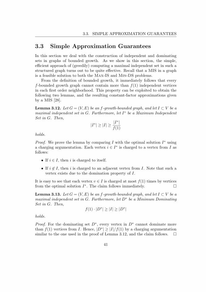
3.3. SIMPLE APPROXIMATION GUARANTEES
3.3 Simple Approximation Guarantees
In this section we deal with the construction of independent and dominatingsets in graphs of bounded growth. As we show in this section, the simple,efficient approach of (greedily) computing a maximal independent set in such astructured graph turns out to be quite effective. Recall that a MIS in a graphis a feasible solution to both the Max-IS and Min-DS problems.
From the definition of bounded growth, it immediately follows that everyf -bounded growth graph cannot contain more than f(1) independent verticesin each first order neighborhood. This property can be exploited to obtain thefollowing two lemmas, and the resulting constant-factor approximations givenby a MIS [28].
Lemma 3.12. Let G = (V,E) be an f-growth-bounded graph, and let I ⊂ V be amaximal independent set in G. Furthermore, let I∗ be a Maximum IndependentSet in G. Then,
|I∗| ≥ |I| ≥ |I∗|f(1)
holds.
Proof. We prove the lemma by comparing I with the optimal solution I∗ usinga charging argumentation. Each vertex i ∈ I∗ is charged to a vertex from I asfollows:
• If i ∈ I, then i is charged to itself.
• If i 6∈ I, then i is charged to an adjacent vertex from I. Note that such avertex exists due to the domination property of I.
It is easy to see that each vertex v ∈ I is charged at most f(1) times by verticesfrom the optimal solution I∗. The claim follows immediately.
Lemma 3.13. Let G = (V,E) be an f-growth-bounded graph, and let I ⊂ V be amaximal independent set in G. Furthermore, let D∗ be a Minimum DominatingSet in G. Then,
f(1) · |D∗| ≥ |I| ≥ |D∗|holds.
Proof. For the dominating set D∗, every vertex in D∗ cannot dominate morethan f(1) vertices from I. Hence, |D∗| ≥ |I|/f(1) by a charging argumentationsimilar to the one used in the proof of Lemma 3.12, and the claim follows.
41

CHAPTER 3. WIRELESS COMMUNICATION GRAPHS
A maximal independent set is thus a constant-factor approximation for theMax-IS and Min-DS problems on graphs of bounded growth. We point outthat any Maximum Independent Set is also maximal. As an interesting remark,note that the cardinalities of optimal solutions to the Max-IS and Min-DS
problems are therefore only a factor of f(1) apart from each other in graphswith f -bounded growth.
A maximal independent set can be created by a greedy strategy as presentedin Section 2.4. When considering a greedy strategy, the choice of the next vertexto be added to a partial solution can be arbitrary. However, for certain classesof graphs, a more sophisticated choice improves the approximation guaranteebelow the value of f(1) for the Max-IS problem.
An example for such an improved choice can be found in Unit Disk Graphs.For a UDG G = (V,E), let pv = (xv, yv) ∈ R
2 denote the position of each vertexv ∈ V in a geometric representation. A possible ordered choice of vertices to beadded to a partial solution I is given by the following criterion:
Choose v ∈ V such that xv = minxu | u ∈ V \ Γ(I).In other words, we always choose a leftmost vertex which is neither in thepartial solution, nor dominated by it. Further on we refer to this approach asLeftmost-Greedy for Unit Disk Graphs.
For the chosen vertex, we now have the following geometric observation,which is also presented in Figure 3.2 [41].
Lemma 3.14. Let G = (V,E) be a UDG with representation pv = (xv, yv)for every v ∈ V , and be v ∈ V such that xv = minxu | u ∈ V . Then, thecardinality of an independent set in Γ(v) is at most 3.
Proof. Let v1, v2 ∈ Γ(v) be two vertices such that (v1, v2) 6∈ E, that is, both‖pv − pvi
‖ ≤ 1, i = 1, 2, and ‖pv1− pv2
‖ > 1 hold. Looking at the two rays ema-nating from pv to pv1
and pv2, a straightforward geometric argumentation shows
that the angle between these two rays has to be larger than π/3. Otherwise,two circles of unit diameter centered at pv1
and pv2intersect.
With this observation, suppose there are 4 independent vertices in the neigh-borhood of v, say v1, . . . , v4 ∈ Γ(v). W.l.o.g. let the vertices be ordered as seenfrom pv. All angles between rays to the positions pv1
, . . . , pv4have to be larger
than π/3. Thus, the overall angle at pv between pv1and pv4
is larger than π,and this contradicts xv being the smallest x-coordinate.
By a small modification to the analysis of Lemma 3.12, that is, charging eachvertex from the partial solution at the time it is chosen by the Leftmost-Greedy,
42

3.3. SIMPLE APPROXIMATION GUARANTEES
v
v1
v2
v3
v4
π/3
π/3
π/3
v1
v2
v3
v
v4
Figure 3.2: Leftmost-Greedy : the vertex v with smallest x-coordinate cannothave more than 3 independent neighbors.
each vertex is charged at most by three independent vertices from an optimalsolution in its neighborhood. Overall, we obtain a 3-approximation with thisapproach.
Another example of a better approximation guarantee by a more sophisti-cated greedy choice can be found in Disk Graphs of arbitrary radius. Let rv
denote the radius of the respective disk centered at the position pv of each ver-tex v ∈ V . A possible ordered choice of vertices to be added next to a partialsolution I during a greedy approach is given by:
Choose v ∈ V such that rv = minru | u ∈ V \ Γ(I).
Similar to the proof of Lemma 3.14, we can geometrically motivate that a cen-ter disk cannot be surrounded by more than 5 disks of equal or larger radiuswhich on one hand intersect with this central disks, but on the other hand donot intersect with each other (see Figure 3.3). Therefore, we can adjust theargumentation so that a disk chosen in this ordered greedy approach is chargedby at most 5 disks with larger radius. This Smallest-Radius-Greedy approachthen gives a 5-approximation for the Max-IS problem on Disk Graphs, and itdoes so for every bound on the ratio between largest and smallest disks in the
43
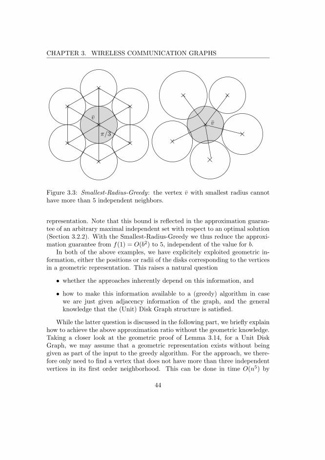
CHAPTER 3. WIRELESS COMMUNICATION GRAPHS
π/3
vv
Figure 3.3: Smallest-Radius-Greedy : the vertex v with smallest radius cannothave more than 5 independent neighbors.
representation. Note that this bound is reflected in the approximation guaran-tee of an arbitrary maximal independent set with respect to an optimal solution(Section 3.2.2). With the Smallest-Radius-Greedy we thus reduce the approxi-mation guarantee from f(1) = O(b2) to 5, independent of the value for b.
In both of the above examples, we have explicitely exploited geometric in-formation, either the positions or radii of the disks corresponding to the verticesin a geometric representation. This raises a natural question
• whether the approaches inherently depend on this information, and
• how to make this information available to a (greedy) algorithm in casewe are just given adjacency information of the graph, and the generalknowledge that the (Unit) Disk Graph structure is satisfied.
While the latter question is discussed in the following part, we briefly explainhow to achieve the above approximation ratio without the geometric knowledge.Taking a closer look at the geometric proof of Lemma 3.14, for a Unit DiskGraph, we may assume that a geometric representation exists without beinggiven as part of the input to the greedy algorithm. For the approach, we there-fore only need to find a vertex that does not have more than three independentvertices in its first order neighborhood. This can be done in time O(n5) by
44

3.4. GRAPH REPRESENTATIONS AND LOCALIZATION
a complete search over all vertices, together with all choices of 4 neighboringvertices which may then not be mutually independent.
For the general Disk Graph case, we can find a vertex with no more than 5independent neighbors to be added in time O(n7). The complexities of O(n5)and O(n7) can be improved by matrix multiplication techniques as proposedin [15].
The above approaches without representation take significantly longer thanexplicitly exploiting a representation. When the geometric information for theordered greedy strategies is available, we can preprocess the input graph andsort the vertices accordingly to obtain the required order. We therefore explorethe idea of constructing a geometric representation from adjacency informationin the following part.
3.4 Graph Representations and Localization
Important problems in the area of geometrically defined graphs are the ques-tions concerning recognition and reconstruction, both from a theoretical and apractical point of view. Generally speaking, these problems start with an undi-rected graph, where only adjacency information of the edges is given, and thenseek for geometric information, e.g. possible positions of the vertices.
Consider the case of Unit Disk Graphs, where the edges can be encoded bygiving each vertex a position in the Euclidean space, and edges are present be-tween vertices if and only if the unit diameter disks at these positions intersect.Note that in the Leftmost-Greedy algorithm of the previous section, we assumedthat such a representation exists. However, we do not need to exploit any infor-mation of such a representation in the algorithm to obtain the approximationguarantee of 3.
This scenario gives rise to one of the most fundamental problems for geo-metrically defined graphs (and structured subclasses of graphs in general), therecognition problem: given a graph, verify if this graph satisfies the geometricproperties that define the structure.
When only adjacency information is available from a Unit Disk Graph G,it becomes hard to distinguish G from an undirected graph without underlyingstructure. In fact, an efficient algorithm to recognize Unit Disk Graphs can beused to efficiently solve NP-complete problems.
Theorem 3.15. The problem of deciding whether a given graph G = (V,E) isa Unit Disk Graph is NP-hard.
45

CHAPTER 3. WIRELESS COMMUNICATION GRAPHS
The above theorem is proven in [8]: Given an instance C of SAT, a cor-responding graph GC is constructed in polynomial time such that GC has afeasible representation if and only if C is satisfiable, i.e. C is a positive instance.However, even though UDG recognition is a decision problem, the question ofa polynomial size certificate is still open, so that the claim of UDG recognitionbeing NP-complete cannot be justified.
Any polynomial time algorithm computing a representation for a UDG couldbe used in a straightforward way to solve the recognition problem. Thus, weimmediately get the following corollary to Theorem 3.15.
Corollary 3.16. For a UDG G = (V,E), if computing a feasible representationp : V → R
2 can be done in polynomial time, then P = NP holds.
Due to this fact, approximations to the problem of computing a represen-tation, which are usually referred to as embedding of a graph come into thepicture. Consider a general, undirected graph G = (V,E) together with somemapping p : V → R
2 which gives each vertex a position in the Euclidean space.We define the quality qp of the embedding p as
qp(G) :=max(u,v)∈E ‖pu − pv‖min(u,v) 6∈E ‖pu − pv‖
.
In case of the geometrically defined wireless communication graphs of the pre-ceding section, this measure captures the essence of wireless communications:the smaller qp, the closer we get to the characteristic that vertices which areclose to one another can communicate directly, and vertices far apart cannot.
It is easy to see that an embedding p with quality qp(G) ≥ 1 defines a QuasiDisk Graph with parameter b = qp as defined in Section 3.2.2. For a UnitDisk Graph G = (V,E), it is also easy to verify that an embedding p∗ is arepresentation of G if and only if qp∗(G) < 1 holds.
A more detailed look at the construction of the graph GC used in the proofof Theorem 3.15, this time in light of the above measure, gives the followingresult [34].
Theorem 3.17. Let G = (V,E) be a Unit Disk Graph. If P 6= NP, then thereis no efficient algorithm that computes an embedding p : V → R
2 with qualityqp(G) ≤
√
3/2 − ε, where ε tends to 0 as |V | → ∞.
On the other hand, in [42], an O(log2.5 n√
log log n)-approximation algorithmfor the embedding of a Unit Disk Graph is proposed.
46

3.5. ROBUST ALGORITHMS
Despite being challenging from a theoretical point of view, also in practice,these questions play an important role in wireless networks. In this area, giv-ing each wireless device its position in the physical environment is known aslocalization. However, practicable, reliable localization in wireless networks isa non-trivial task [56], and there are numerous in-network approaches to thisproblem proposed in the literature. These are then usually evaluated numeri-cally in ideal settings. Furthermore, for example after the initial employmentof a wireless sensor network, positional information may not yet be available.Nevertheless, in this setting, efficient communication structures—including in-dependent and dominating sets—need to be set up as well. Of course, a ratherquick—yet expensive—solution is to equip each device with a GPS or Galileoreceiver.
3.5 Robust Algorithms
From the above discussion, it becomes clear that in wireless communicationgraphs, the question of geometric representation or localization is an importantone. The information how a graph is presented as input to an algorithm, e.g.by its adjacency information only, or by its complete geometric representation,determine significant differences in the design of optimization algorithms.
In this context, when a geometric representation is not available, the notionof robustness comes into play. Generally speaking, a robust algorithm mustproduce correct output regardless of the input [53]. More precisely, robustalgorithms on a subset of instances of a problem are defined as follows.
Definition 3.18. Let A be an algorithm defined on a set I of instances, andlet f be a function defined on I. Furthermore, let U ⊆ I.
Then, we say that A computes f robustly (on U ⊆ I) if
• for all instances x ∈ U , the algorithm A returns f(x), and
• for all instance x ∈ I \ U , the algorithm A returns either f(x), or acertificate showing that x 6∈ U .
Of course, the notion of a robust algorithm is especially interesting whenA has polynomial running time with respect to the size of the input, and thedecision whether an instance belongs to the subclass U ⊆ I is not easy to decide.
For example, keeping Theorem 3.15 in mind, an algorithm A may robustlycompute some function f on Unit Disk Graphs, and accept any undirected graphas input. An output then either gives a value for f , or a certificate that the
47

CHAPTER 3. WIRELESS COMMUNICATION GRAPHS
input is not a Unit Disk Graph. Note that, in case a value for f is returned, wemay not conclude that the input is a Unit Disk Graph. However, A computedthe correct value for f .
Furthermore, robust algorithms can be combined in sequence, where thecomputed solution is used as input for further algorithms, that is, as buildingblocks of more general algorithms. In other words, robustness is preserved bycomposition. This is to be contrasted to the non-robust case where an algorithmneed not produce an output or even terminate if the input does not satisfy theadditional structural properties, and some produced output may not even be afeasible solution to the problem at hand.
3.6 Conclusions
In this chapter, we have reviewed and proposed geometrically inspired con-tainment and intersection graph models for communication in wireless, ad-hocnetworks. These range from ideal assumptions, resulting in a Unit Disk Graph,to more realistic approaches, resulting in Bounded Area Graphs. All these graphmodels have in common the structure of polynomially bounded growth if therespective parameters are bounded.
The bounded growth property allows for a constant-factor bound on the ra-tio between the cardinalities of maximal independent sets and optimal solutionsto the Max-IS and Min-DS problems respectively. Furthermore, since a Max-imum Independent Set is also maximal, this ratio also holds between optimalsolutions to these two problems on the same instance.
For the geometric intersection graphs, possibly exploiting geometric infor-mation, we can further improve the approximation ratio given by a maximalindependent set for some classes of graphs. We have seen that having a geo-metric representation available differs greatly from the case that we only haveadjacency information. The questions of embedding, or localization, were dis-cussed. We also introduced the notion of robust algorithms. These type ofalgorithms present a way to deal with optimization on the presented subclassesof undirected graphs.
In the following, since bounded growth is a structural property of a graph,we assume the growth function or polynomial to be known, and not part of theinput. This is reasonable as the actual graph is an instance of the optimizationproblems we are considering, whereas the growth function is defined for possibleinstances reflecting wireless communication graphs.
48

Chapter 4
Polynomial-TimeApproximation Schemes
This chapter presents polynomial-time approximation schemes forMaximum Independent Set and Minimum Dominating Set problemson polynomially Bounded Growth Graphs.We briefly introduce the algorithms for Unit Disk Graphs which relyon a given geometric representation. The main focus, however, lieson an approach called local neighborhood-expansion scheme, that nolonger relies on a geometric representation but only requires poly-nomially bounded growth.The presented approach can be extended towards a robust algorithmthat works on any undirected graph and either returns a subset of de-sired quality, or gives a polynomial time certificate showing that theinstance does not reflect a graph of polynomially bounded growth.
49

CHAPTER 4. POLYNOMIAL-TIME APPROXIMATION SCHEMES
In this chapter, we present polynomial-time approximation schemes for theMax-IS and Min-DS problems on graphs of polynomially bounded growth.Recall that a PTAS is a family of algorithms which in addition to an instanceyield a desired approximation guarantee (1 + ε), given by a parameter ε > 0 aspart of the input. The run time, for fixed ε, has to be polynomial.
We start by introducing main concepts that yield existing PTASs on ge-ometrically defined graphs such as Unit Disk Graphs, and that explicitely re-quire geometric information. While these approaches have been known for sometime, the question whether there is also an approach for the case that a geo-metric representation is not available, was an open problem. As we have seenin Section 3.4, this non-geometric case is significantly more difficult due to thehardness of computing a feasible representation. We thus abandon the geome-try thereafter and focus on graphs of polynomially bounded growth, which alsoincludes an answer to this question.
For these polynomial BGGs, we present an approach based on adjacencyinformation only that yields PTASs for the Max-IS and Min-DS problems.The resulting algorithms work free of any geometric information, and thus givea positive answer to the above question of a PTAS without representation.The approach for both problems constructs optimal, partial solutions for locallybounded neighborhoods, and combines these to create a globally feasible solu-tion which satisfies the desired approximation guarantee. The algorithms, alsofor the weighted version of the Max-IS problem, are explained in Section 4.2,and follow the ideas of [48] and [47].
Besides the independence from a geometric representation, an additional ad-vantage of the PTAS lies in the fact that we can extend the algorithm towardsa robust approach. We have a polynomial time algorithm which either approxi-mates the problem, or solves the recognition problem. Note that the algorithmdoes not solve the recognition problem in general. If the graph is not geomet-rically defined, it may also return a desired, (1 + ε)-approximate solution. Thisis further discussed in Section 4.3.
4.1 Schemes Based on Geometric Separation
Most of the existing work on approximation schemes for wireless communicationgraphs is reported for (Unit) Disk Graphs, and assume the graph given by itsgeometric representation. We would like to point out again that both Max-IS
and Min-DS problems are NP-hard even when the input is restricted to UnitDisk Graphs with a given representation [10]. However, when the representation
50
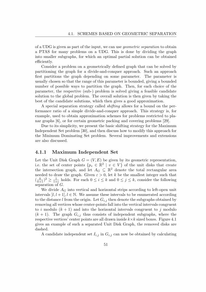
4.1. SCHEMES BASED ON GEOMETRIC SEPARATION
of a UDG is given as part of the input, we can use geometric separation to obtaina PTAS for many problems on a UDG. This is done by dividing the graphinto smaller subgraphs, for which an optimal partial solution can be obtainedefficiently.
Consider a problem on a geometrically defined graph that can be solved bypartitioning the graph for a divide-and-conquer approach. Such an approachfirst partitions the graph depending on some parameter. The parameter isusually chosen so that the range of this parameter is bounded, giving a boundednumber of possible ways to partition the graph. Then, for each choice of theparameter, the respective (sub-) problem is solved giving a feasible candidatesolution to the global problem. The overall solution is then given by taking thebest of the candidate solutions, which then gives a good approximation.
A special separation strategy called shifting allows for a bound on the per-formance ratio of a simple divide-and-conquer approach. This strategy is, forexample, used to obtain approximation schemes for problems restricted to pla-nar graphs [6], or for certain geometric packing and covering problems [29].
Due to its simplicity, we present the basic shifting strategy for the MaximumIndependent Set problem [30], and then discuss how to modify this approach forthe Minimum Dominating Set problem. Several improvements and extensionsare also discussed.
4.1.1 Maximum Independent Set
Let the Unit Disk Graph G = (V,E) be given by its geometric representation,i.e. the set of center points pv ∈ R
2 | v ∈ V of the unit disks that createthe intersection graph, and let AG ⊆ R
2 denote the total rectangular areaneeded to draw the graph. Given ε > 0, let k be the smallest integer such that( k
k+1 )2 ≥ 11+ε holds. For each 0 ≤ i ≤ k and 0 ≤ j ≤ k, consider the following
separation of G.We divide AG into vertical and horizontal strips according to left-open unit
intervals ]l, l + 1], l ∈ N. We assume these intervals to be enumerated accordingto the distance l from the origin. Let Gi,j then denote the subgraphs obtained byremoving all vertices whose center-points fall into the vertical intervals congruentto i modulo (k + 1) and into the horizontal intervals congruent to j modulo(k + 1). The graph Gi,j thus consists of independent subgraphs, where therespective vertices’ center points are all drawn inside k×k sized boxes. Figure 4.1gives an example of such a separated Unit Disk Graph, the removed disks aredashed.
A candidate independent set Ii,j in Gi,j can now be obtained by calculating
51

CHAPTER 4. POLYNOMIAL-TIME APPROXIMATION SCHEMES
1 2 3 4 5 6 7 8 9 10 11 12 13 14 15 16 17
1
2
3
4
5
6
7
8
Figure 4.1: Separated representation of a UDG (k = 3, i = 3, j = 0), Max-IS
case.
a Maximum Independent Set in all boxes separately. For each box, the size ofany independent set therein is bounded by the area O(k2) by a simple pack-ing argument of non-overlapping disks similar to Theorem 3.5. Therefore, anoptimal solution Ii,j can be computed in nO(k2), e.g. by complete enumeration.
Each of the solutions Ii,j forms a candidate for an approximation of theMaximum Independent Set in G. Let I be the largest set among these can-didate sets, i.e. |I| := maxi,j |Ii,j |, which is returned as overall solution. Adetailed summary of the approach to compute I is given by Algorithm 3, andthe following theorem establishes the (1 + ε) approximation guarantee.
Theorem 4.1. Let I∗ be a Maximum Independent Set in a UDG G = (V,E).The set I computed by Algorithm 3 is independent and satisfies
(1 + ε) · |I| ≥ |I∗|.
Proof. Clearly, by the separation of the boxes, each Ii,j consists of separatedindependent sets inside the boxes, and the solution I is thus an independentset.
Consider the vertical separation, and let Gi be the resulting graph For eachi = 0, . . . , k, let Si denote the set of removed vertices, i.e. Si := V (G \ Gi).
Observe that, for 0 ≤ i1 < i2 ≤ k, we have Si1 ∩ Si2 = ∅, and⋃k
i=0 Si = V .
52
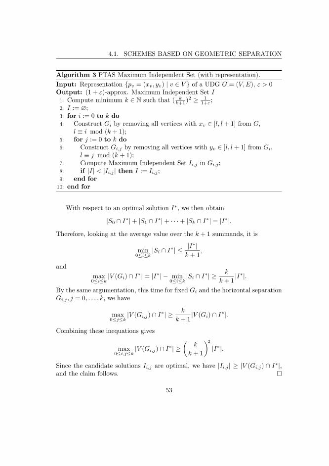
4.1. SCHEMES BASED ON GEOMETRIC SEPARATION
Algorithm 3 PTAS Maximum Independent Set (with representation).
Input: Representation pv = (xv, yv) | v ∈ V of a UDG G = (V,E), ε > 0Output: (1 + ε)-approx. Maximum Independent Set I1: Compute minimum k ∈ N such that ( k
k+1 )2 ≥ 11+ε ;
2: I := ∅;3: for i := 0 to k do4: Construct Gi by removing all vertices with xv ∈ ]l, l + 1] from G,
l ≡ i mod (k + 1);5: for j := 0 to k do6: Construct Gi,j by removing all vertices with yv ∈ ]l, l + 1] from Gi,
l ≡ j mod (k + 1);7: Compute Maximum Independent Set Ii,j in Gi,j ;8: if |I| < |Ii,j | then I := Ii,j ;9: end for
10: end for
With respect to an optimal solution I∗, we then obtain
|S0 ∩ I∗| + |S1 ∩ I∗| + · · · + |Sk ∩ I∗| = |I∗|.
Therefore, looking at the average value over the k + 1 summands, it is
min0≤i≤k
|Si ∩ I∗| ≤ |I∗|k + 1
,
and
max0≤i≤k
|V (Gi) ∩ I∗| = |I∗| − min0≤i≤k
|Si ∩ I∗| ≥ k
k + 1|I∗|.
By the same argumentation, this time for fixed Gi and the horizontal separationGi,j , j = 0, . . . , k, we have
max0≤j≤k
|V (Gi,j) ∩ I∗| ≥ k
k + 1|V (Gi) ∩ I∗|.
Combining these inequations gives
max0≤i,j≤k
|V (Gi,j) ∩ I∗| ≥(
k
k + 1
)2
|I∗|.
Since the candidate solutions Ii,j are optimal, we have |Ii,j | ≥ |V (Gi,j) ∩ I∗|,and the claim follows.
53

CHAPTER 4. POLYNOMIAL-TIME APPROXIMATION SCHEMES
1
2
3
4
5
6
7
8
1 2 3 4 5 6 7 8 9 10 11 12 13 14 15 16 170
0
Figure 4.2: Separated representation of a UDG (k = 3, i = 1, j = 0), Min-DS
case.
Clearly, Algorithm 3 has polynomial run time, which is dominated by thecomputation of the (k+1)2 different candidate solutions Ii,j in time nO(k2). Notethat k is bounded depending on ε. Also, an extension to higher dimensions isstraightforward. Furthermore, it is easy to adapt the algorithm and the aboveproof to the weighted version of the problem, by replacing the cardinality of thesubsets with their respective weight.
There are several improvements to the above generic separation approach.By applying dynamic programming techniques along one of the separating di-mensions, the time bound can be reduced to nO(k) by giving an optimal solutionin Gi for each i = 0, . . . , k. This idea can be extended to geometric objects inR
d, d ≥ 2, whose projection to the first d−1 coordinates have roughly the samesize, e.g. for map labeling problems treated in [1]. Combined with a dynamicprogramming approach which simultaneously considers disks of different size,the shifting strategy also yields a PTAS for General Disk Graphs [16], thus nolonger requiring the disks to have roughly the same radii.
4.1.2 Minimum Dominating Set
The geometric separation approach can also be used to obtain a PTAS for theMinimum Dominating Set problem on UDGs. We now present a basic (k+2
k )2-approximation algorithm also using the shifting strategy. The parameter k ∈ N
54

4.1. SCHEMES BASED ON GEOMETRIC SEPARATION
u2u1
v
B
Figure 4.3: Using v 6∈ B as dominating vertex for u1, u2 ∈ B.
is then chosen so that (k+2k )2 ≤ (1 + ε) holds.
For the dominating set approach, there are some subtle differences to a PTASfor maximum independent sets:
• Geometric separation cannot be done by removing vertices from horizontaland vertical strips. A subset of a dominating set no longer needs to bedominating. Therefore, we separate along horizontal lines at l ≡ i mod kand vertical lines at t ≡ j mod k (Figure 4.2). This yields boxes of theform ]l, l + k]×]t, t + k], and for fixed i, j, the boxes form a partition of G.This way, it is ensured that each vertex in G is dominated.
• A minimum cardinality set dominating the vertices of a box B, say e.g.B = ]l, l+k]×]t, t+k] for some l and t, may contain vertices from adjacentstrips: A vertex v ∈ V , with pv 6∈ B, but whose unit disk intersectswith disks centered inside B can be used to dominate these vertices, seeFigure 4.3.
So, for the computation of an optimal dominating set for a k × k sized box,we have to consider adjacent vertices, as well. For the construction of a partialsolution, we expand each box by one unit in each direction, that is, we may usevertices from this expanded (k + 2) × (k + 2) sized box to dominate verticesinside the k × k sized box.
The construction of the candidate solution Di,j for a set of boxes Bi,j canstill be done efficiently. Any maximal independent set in a k × k sized boxis of cardinality O(k2), and by Theorem 2.10, such a set is also dominating.Thus, even considering an enlarged box for an optimal dominating set, thecardinality of such a set remains O(k2), and can be constructed, e.g. by complete
enumeration in nO(k2). Due to k being bounded depending on ε, the overall runtime of the algorithm is thus polynomial.
Algorithm 4 presents the modified PTAS for the Min-DS problem on UDGs
55

CHAPTER 4. POLYNOMIAL-TIME APPROXIMATION SCHEMES
Algorithm 4 PTAS Minimum Dominating Set (with representation).
Input: Representation pv = (xv, yv) | v ∈ V of a UDG G = (V,E), ε > 0Output: (1 + ε)-approx. Minimum Dominating Set D1: Compute minimum k ∈ N such that (k+2
k )2 ≤ 1 + ε;2: D := ∅;3: for i := 0 to k − 1 do4: for j := 0 to k − 1 do5: Partition V along the k × k sized boxes yielding sets Bi,j :=
v ∈ V | pv ∈ ]l, l + k]×]t, t + k], l ≡ i mod k, t ≡ j mod k;6: For each B ∈ Bi,j , compute a Minimum Dominating Set for B in G,
and combine these to Di,j ;7: if |D| > |Di,j | then D := Di,j ;8: end for9: end for
with representation. For the quality of the solution, we have the followingtheorem.
Theorem 4.2. For a UDG G = (V,E), let D∗ denote a Minimum DominatingSet of G. Then, Algorithm 4 constructs a dominating set D of cardinality
|D| < (1 + ε) · |D∗|.
Proof. It is easy to see that D dominates V since the k× k sized boxes for eachchoice of i and j are cover the entire graph.
Consider the vertical separation only. Then, for some iteration 0 ≤ i′ < k,at most 2
k · |D∗| vertices fall into the additional unit intervals left and right ofthe lines that partition the graph. This is due to the fact that each vertical unitinterval, over all k iterations, is considered at most once left of each strip, andat most once right of each vertical strip of width k.
The cardinality of the dominating set for all these strips, given by the unionof the optimal dominating sets for each extended strip ]l − 1, l + k + 1] withl ≡ i′ mod k, is then no more than |D∗| + 2
k · |D∗| = k+2k · |D∗|.
By the same argumentation, we can obtain a (k+2k )-approximate dominating
set inside each of the above horizontal strips, and sequential application yieldsthe claim.
Again, from the proof, an extension to higher dimensions is straightforward.A slightly modified algorithm with adjacent k × k sized boxes gives a PTAS
56

4.2. LOCAL NEIGHBORHOOD BASED SCHEMES
for the Minimum Vertex Cover problem [30]. For the weighted dominating set,this approach is no longer applicable due to the fact that the cardinality of aweighted dominating set inside a box can no longer be bounded. In [9], theabove approach is extended towards the Minimum Connected Dominating Setproblem.
4.2 Local Neighborhood Based Schemes
As seen in Section 3.4, the case when no geometric representation is available issignificantly different already for UDGs. We cannot easily make this informationavailable to an algorithm. Next, we go on to present an approach that no longerrelies on positional information of the vertices, but assumes only knowledge ofthe adjacency of each vertex in the graph. Additionally, we no longer restrictthe discussion to UDGs, but assume the graph G = (V,E) to be of polyno-mially bounded growth, thus completely abandoning any underlying geometricstructure.
The following discussion follows [48] and [47], where robust PTASs for theMax-IS and Min-DS problems respectively are presented for UDGs withoutgeometric representation. In order to simplify the presentation of the approxi-mation schemes, we introduce some definitions and notation, including the basicdefinition of collections of d-separated neighborhoods in G.
Definition 4.3. For a graph G = (V,E), let S = S1, . . . , Sk be a collectionof subsets of vertices Si ⊆ V, i = 1, . . . , k, with the following property:
for any two vertices s ∈ Si and s ∈ Sj , i 6= j, dG(s, s) > d.
We refer to S as a d-separated collection of subsets.
It is easy to see that the subsets of any d-separated collection, d ≥ 0, aremutually disjoint. We call a d-separated collection S = S1, . . . , Sk exhaustiveif for every vertex v ∈ V , there exists a vertex s ∈ ⋃
Si such that dG(v, s) ≤ d.An example of an exhaustive 2-separated collection is given in Figure 4.4. Thegrey areas mark the different subsets that make up the collection; vertices whichare not part of it, and thus separate the subsets, are white.
Denote by P(V ) the set of all subsets of vertices. We then define two func-tions I : P(V ) → P(V ) and D : P(V ) → P(V ) which return an independentset of maximum cardinality and a dominating set of minimum cardinality re-spectively for the subset given as argument. For a subset V ′ ⊆ V , the set
57

CHAPTER 4. POLYNOMIAL-TIME APPROXIMATION SCHEMES
S5
S6
S4S2
S3
S1
Figure 4.4: Example of a 2-separated collection S = S1, . . . , S6
I(V ′) is independent in V ′, and D(V ′) dominates V ′. For D(V ′), the inclusionD(V ′) ⊆ V ′ needs not to hold. Therefore, in the following, the function D(.) isalways computed with respect to the entire underlying graph G. However, it iseasy to see that V ′ ⊆ Γ(D(V ′)) and that D(V ′) ⊆ Γ(V ′) hold.
Using the above definitions, we are thus interested in a polynomial timeapproximation of I(V ) and D(V ) within a factor of 1+ε for any given ε > 0. Dueto the intractability of the corresponding optimization problems, we resort toan implicit divide-and-conquer approach using local neighborhoods and partialsolutions therein.
For some vertex v ∈ V , and its r-th neighborhood Γr(v), we use Ir(v) andDr(v) to denote the independent set I(Γr(v)) and the dominating set D(Γr(v))for Γr(v). Further on, in case the vertex v is unambiguous, we omit indexingthe respective neighborhoods and subsets with this central vertex.
Suppose the radius r of a neighborhood Γr is bounded. Then by the definitionof Bounded Growth Graphs, and the fact that any maximal independent set isalso dominating (Theorem 2.10),
|Dr| ≤ |Ir| ≤ p(r)
holds. With this bound on the cardinality of the locally optimal solutions, it
58

4.2. LOCAL NEIGHBORHOOD BASED SCHEMES
becomes clear that we can obtain both optimal solutions Ir and Dr in timenO(p(r)) for this neighborhood Γr.
4.2.1 Maximum Independent Set
We now present an approach that gives the PTAS for the Maximum IndependentSet problem on a polynomial BGG G = (V,E). The basic idea of is simple. Westart with an arbitrary vertex v ∈ V , and consider for r = 0, 1, 2, . . . , the r-thneighborhoods Γr(v) = Γr and optimal independent sets Ir(v) = Ir ⊆ Γr therein.
We keep expanding the neighborhoods as long as
|Ir+1| > (1 + ε) · |Ir|
holds. Let r denote the smallest r ≥ 0 for which this condition is violated. Suchan r indeed exists, and it is bounded by a constant that only depends on ε.
Lemma 4.4. Let G = (V,E) be a graph of polynomially p-bounded growth.There exists a constant c = c(ε) such that r ≤ c.
Proof. Let r < r. By definition of r, we then have for r
|Ir| > (1 + ε)|Ir−1| > · · · > (1 + ε)r|I0| = (1 + ε)r.
Since the graph G is of polynomial bounded growth, we also have |Ir| ≤ p(r).By comparison, i.e.
p(r) ≥ |Ir| > (1 + ε)r,
the claim follows.
To achieve an independent set for the graph G, we iteratively apply the abovescheme. Each time the expansion is stopped, we remove the neighborhoodΓr+1 from G, and combine Ir with the partial solution I obtained thus far.Since Ir ⊆ Γr, while we remove Γr+1, the set Γr is 1-separated to all sets tobe calculated in the remaining process. This implies that the created sets Γr
during the complete algorithm form a 1-separated collection. This collection ofsubsets is also exhaustive since we continue creating partial solutions until theremaining graph is empty.
A detailed summary of the above approach is given by Algorithm 5, and wenow prove its correctness and polynomial complexity starting with the indepen-dence property of the returned solution.
59

CHAPTER 4. POLYNOMIAL-TIME APPROXIMATION SCHEMES
Algorithm 5 PTAS Maximum Independent Set.
Input: G = (V,E) polynomial BGG, ε > 0Output: (1 + ε)-approx. Maximum Independent Set I1: I := ∅;2: while V 6= ∅ do3: Pick v ∈ V ;4: r := 0;5: while |Ir+1(v)| > (1 + ε) · |Ir(v)| do6: r := r + 1;7: end while8: I := I ∪ Ir(v);9: V := V \ Γr+1(v);
10: end while
Lemma 4.5. The solution I created by Algorithm 5 forms an independent setin the graph G.
Proof. This follows directly from the separation of the neighborhoods consid-ered: each v ∈ V \ Γr+1 has no neighbor in Γr, and thus not in Ir ⊆ Γr.
In order to motivate that all operations can be completed in polynomial runtime, note that we only need to consider a single iteration, as the number of newcentral vertices picked in the algorithm is limited by n. Due to the definition ofa polynomial BGG, and the constant established by Lemma 4.4, every operationcan be completed in polynomial time, with the degree only depending on ε > 0,but not on the size of the graph. It remains to show that the cardinality of theindependent set I meets the desired approximation guarantee of (1 + ε).
Theorem 4.6. Let I∗ := I(V ) be a Maximum Independent Set in a polynomialBGG G = (V,E). The independent set I computed by Algorithm 5 satisfies
(1 + ε) · |I| ≥ |I∗|.
Proof. Suppose inductively that Algorithm 5 computes a (1 + ε)-approximateindependent set I ′ ⊆ V \ Γr+1 for G′ = G[V \ Γr+1].
By definition of r, we have
|Ir+1| ≤ (1 + ε) · |Ir|.
60

4.2. LOCAL NEIGHBORHOOD BASED SCHEMES
Since the cardinality of the part of the optimal set I∗ which lies in G[Γr+1] isbounded by the cardinality of Ir+1, we get
|Γr+1 ∩ I∗| ≤ |Ir+1| ≤ (1 + ε) · |Ir|.
Further, by inductive assumption, I ′ is (1 + ε)-approximately optimal for G′.Therefore,
|V (G′) ∩ I∗| ≤ |I(V (G′))| ≤ (1 + ε) · |I ′|.Adding the two inequalities, we obtain
|I∗| ≤ (1 + ε) · (|Ir| + |I ′|) = (1 + ε) · |I|.
Note that the Algorithm 3 actually returns a (1 + ε)-approximate indepen-dent set for any undirected graph given as input. We have only used the specificstructure of polynomial BGGs in Lemma 4.4 in order to bound the radius ofthe largest neighborhood we need to consider during execution. The criterionto stop expanding a neighborhood is met eventually in any undirected graph,however, possibly while considering an O(n)-neighborhood or eventually G it-self.
Coming back to the run time of Algorithm 5, we see that the time needed forcompletion of the algorithm is dominated by the constant c = c(ε) of Lemma 4.4.To be more precise, the run time dominated by the time needed to construct anoptimal solution for Γr+1(v), r ≤ c.
Using the inequality log(1+ε) > 1/2 ·ε for sufficiently small ε, we can boundthe constant c by O(1/ε log 1/ε). The overall run time of the approach is thusnO(1/ε log 1/ε).
4.2.1.1 Maximum Weight Independent Set
The previous approximation scheme can easily be adapted for the case that eachvertex v ∈ V is given a weight wv. Without loss of generality, we assume wv > 0for every v ∈ V . Recall that in this case, we are interested in an independent setI ⊆ V of high total weight W (I) :=
∑
i∈I wi in G. We now present the necessarymodifications to the previous algorithm in order to obtain an independent setof weight at least (1 + ε)−1 the maximum total weight of any independent setin the polynomial BGG.
The algorithm again follows the idea of expanding the local neighborhoodof a central vertex v. This time, however, the central vertex v is chosen to be
61

CHAPTER 4. POLYNOMIAL-TIME APPROXIMATION SCHEMES
a vertex with maximum weight wv = maxwi | i ∈ V in the remaining graphG. Then, we compute an independent set Ir ⊆ Γr(v) of maximum weight forincreasing radii r until the criterion
W (Ir+1) > (1 + ε) · W (Ir)
is violated. Let r denote the smallest r ≥ 0 for which this is the case.
Lemma 4.7. Let G = (V,E) be a p-BGG. There exists a constant c = c(ε)such that r ≤ c.
Proof. Adapting the proof of Lemma 4.4, for r < r we get
W (Ir) =∑
i∈Ir
wi ≤∑
i∈Ir
wmax = |Ir| · wmax,
and
W (Ir) > (1 + ε) · W (Ir−1) > . . . > (1 + ε)r · W (I0) = (1 + ε)r · wmax
respectively. Since |Ir| ≤ p(r), combining the above two inequalities again yieldsthe claim.
As a consequence, the running time of this algorithm remains polynomial inthe weighted case. Furthermore, the approximation ratio can be guaranteed bythe following theorem.
Theorem 4.8. The adapted algorithm, i.e. choosing a central vertex of maxi-mum weight in G in each round, creates an independent set I of weight
(1 + ε) · W (I) ≥ W (I∗),
where I∗ denotes an optimal solution to the Maximum Weight Independent Setproblem on G.
Proof. Let V ′ := V \ Γr+1(v), and assume inductively that I ′ ⊆ V ′ is a (1 + ε)-approximate weighted independent set in G[V ′]. Clearly, Ir ∪ I ′ is an indepen-dent set in G.
For the weighted independent set in the neighborhood Γr+1(v), we have
W (I∗ ∩ Γr+1(v)) ≤ W (Ir+1) ≤ (1 + ε) · W (Ir)
from the criterion to stop expanding the neighborhoods.
62

4.2. LOCAL NEIGHBORHOOD BASED SCHEMES
For the weight W (I) = W (Ir ∪ I ′) of the overall solution set I returned bythe algorithm we then get
W (I∗) = W ((I∗ ∩ Γr+1(v) ∪ (I∗ ∩ V ′))
= W (I∗ ∩ Γr+1(v)) + W (I∗ ∩ V ′)
≤ (1 + ε) · W (Ir) + (1 + ε) · W (I ′)
= (1 + ε) · W (Ir ∪ I ′)
= (1 + ε) · W (I).
Summarizing, we have the following corollary for independent sets on graphsof polynomially bounded growth.
Corollary 4.9. There exists a PTAS for the Maximum (Weight) IndependentSet problem on graphs of polynomially bounded growth. In addition to the desiredapproximation guarantee, this PTAS requires only adjacency information of theinput graph.
4.2.2 Minimum Dominating Set
In this part, we present a polynomial-time approximation scheme for the Min-imum Dominating Set problem on graphs of polynomially p-bounded growth.The approach follows the implicit separation idea of the PTAS for the Max-IS
problem on this class of graphs presented in Section 4.2.1. However, while in theprevious section, the separation strategy and the overall approximation followedby rather simple arguments, for the Min-DS problem, some attention has to bepaid to the manner the local neighborhoods are created and put together.
Again, we use local neighborhoods of bounded radius, and optimal partialsolutions therein, to obtain a PTAS. Recall that for neighborhoods Γr(v), v ∈ V,in graphs of polynomially p-bounded growth, we can obtain a dominating setDr(v) = D(Γr(v)) of minimum cardinality in time nO(p(r)).
The main part of the algorithm now consists of iteratively constructing dom-inating sets for the local neighborhoods Γr, and to stop if the cardinality of thesedominating sets does not grow too much any more. To be more precise, we stopexpanding the radius r of the neighborhoods if
|Dr+2(v)| > (1 + ε) · |Dr(v)|
is violated.
63

CHAPTER 4. POLYNOMIAL-TIME APPROXIMATION SCHEMES
Algorithm 6 PTAS Minimum Dominating Set.
Input: G = (V,E) polynomial BGG, ε > 0Output: (1 + ε)-approx. Minimum Dominating Set D1: D := ∅;2: while V 6= ∅ do3: Pick v ∈ V ;4: r := 0;5: while |Dr+2(v)| > (1 + ε) · |Dr(v)| do6: r := r + 1;7: end while8: D := D ∪ Dr+2(v);9: V := V \ Γr+2(v);
10: end while
Recall the possibility of vertices outside a subset being able to dominatevertices inside this subset. The local dominating sets are always created withrespect to G, for neighborhoods Γr, we have Dr ⊆ Γr+1. Therefore, in order tohave sufficient separation, we need to consider a 2-separated structure given bythe neighborhoods.
The approach constructs a 2-separated collection of neighborhoods given bythe Γr(v), where r denotes the radius upon stopping to expand the neighbor-hoods. At this point, we remove Γr+2 from G and keep Dr+2 as part of thesolution. The overall separation can then easily be seen by inductive argumen-tation: each neighborhood removed from the remaining set V of vertices satisfiesthe separation property with respect to previously removed neighborhoods andthe resulting reduced set V for the following iteration. The resulting algorithmfrom the above approach is given by Algorithm 6.
The following lemma then gives a lower bound for partial dominating setsof 2-separated collections with respect to an optimal dominating set for a graphG.
Lemma 4.10. Let D∗ := D(V ) be a Minimum Dominating Set in a graphG = (V,E). For a 2-separated collection S = S1, . . . , Sk in G, it is
|D∗| ≥k∑
i=1
|D(Si)|.
Proof. For each subset Si ∈ S, consider the neighborhood Γ(Si). As a directconsequence of the definition of 2-separated subsets, these neighborhoods are
64

4.2. LOCAL NEIGHBORHOOD BASED SCHEMES
pairwise disjoint. Furthermore, any vertex outside Γ(Si) has distance more thanone to all vertices in Si. Therefore, D∗ ∩ Γ(Si) dominates Si.
On the other hand, also D(Si) ⊆ Γ(Si) dominates Si using a minimumnumber of vertices. Therefore, we obtain
|D∗ ∩ Γ(Si)| ≥ |D(Si)|.
Combining this observation for all subsets of S, we get
|D∗| ≥k∑
i=1
|D∗ ∩ Γ(Si)| ≥k∑
i=1
|D(Si)|,
as claimed.
Looking at such a 2-separated collection, together with related subsets andbounded cardinality dominating sets for these, we extend the above Lemma 4.10to receive an upper bound.
Corollary 4.11. Let S = S1, . . . , Sk be a 2-separated collection in G =(V,E), and let T1, . . . , Tk be subsets of V with Si ⊆ Ti for all i = 1, . . . , k.If there exists a bound ρ ≥ 1 such that
|D(Ti)| ≤ ρ · |D(Si)|
holds for all i = 1, . . . , k, then the set T :=⋃k
i=1 D(Ti) satisfies
|T | ≤ ρ · |D∗|,
where D∗ denotes a Minimum Dominating Set in G.
Proof. |⋃ki=1 D(Ti)| ≤
∑ki=1 |D(Ti)| ≤ ρ · ∑k
i=1 |D(Si)| ≤ ρ · |D∗|.
The partial solutions taken from the respective (r+2)-neighborhoods Γr+2 ineach iteration thus satisfy the desired approximation guarantee. Furthermore,the following lemma establishes the overall domination property for the partialsolutions D(Γr+2).
Lemma 4.12. The set D returned by Algorithm 6 dominates G = (V,E).
Proof. Let Ni denote the neighborhoods Γr+2(v) removed from V in each iter-ation i = 1, . . . , k of the algorithm. Then, since we stop the algorithm whenV = ∅ is reached, it is
⋃ki=1 Ni = V , and each of these neighborhoods Ni is
dominated by D(Ni). Therefore,⋃k
i=1 D(Ni) dominates G.
65

CHAPTER 4. POLYNOMIAL-TIME APPROXIMATION SCHEMES
So far, we see that the solution set D returned by Algorithm 6 is a global(1 + ε)-approximate dominating set for the input graph G. At this point, itis noteworthy to remind that this approximation guarantee is valid for anyundirected graph G, even if it does not satisfy the bounded growth condition.
It remains to show that the approximation algorithm has polynomial runtime. Clearly, the number of times we have to pick a new central vertex, andconstruct local neighborhoods and dominating sets for these is bounded byn = |V |. We may thus limit the further discussion to one iteration only. Sincea vertex-induced subgraph of a BGG again is a BGG, we focus w.l.o.g. onthe polynomial BGG G = (V,E) in the first iteration, and again show that theradius of the largest neighborhood we need to consider is bounded by a constant.
Lemma 4.13. Let G = (V,E) be a graph of polynomially p-bounded growthgraph. There exists a constant c = c(ε) such that the radius r of any neighbor-hood Γr(v) considered in the algorithm is bounded by c, i.e. r ≤ c.
Proof. It is |D(Γ0(v))| = |D(Γ1(v))| = 1, as the central vertex v dominates itselfand all its neighbors.
Consider the criterion for stopping to expand the neighborhoods in Algo-rithm 6, and consider the inequality |D(Γr+2)| > (1 + ε) · |D(Γr)| for all r ≤ r.
First, if r is an even number, we have
p(r + 2) ≥ |D(Γr+2)| > (1 + ε) · |D(Γr)|> · · · > (1 + ε)r/2 · |D(Γ0)| = (
√1 + ε)r.
Second, if r is odd, we get
p(r + 2) ≥ |D(Γr+2)| > (1 + ε) · |D(Γr)|> · · · > (1 + ε)r/2 · |D(Γ1)| = (
√1 + ε)r.
Since ε > 0, and thus√
1 + ε > 1, in both cases, the inequalities have to be vio-lated eventually. Thus, the bound c on the largest radius of the neighborhoodsdepends only on the approximation guarantee ε.
If the input graph of Algorithm 6 is of polynomially bounded growth, eachiteration has polynomial running time. The complexity of the computation ofD(Γr(v)) dictates the overall run time of the algorithm. This can be achievedin nO(p(c)).
We close this part with the following summary.
66

4.3. ROBUSTNESS
Corollary 4.14. There exists a PTAS for the Min-DS problem on graphs ofpolynomially bounded growth. In addition to the desired approximation guaran-tee, the respective approximation schemes require only adjacency information ofthe input graph.
4.3 Robustness
We now present a simple way to make the above approximation schemes robust.In this case, the robust algorithm accepts any undirected graph as valid input,and either returns a desired approximate solution, or outputs a polynomial cer-tificate showing that the input graph does not satisfy the structural assumptionof p-bounded growth.
Recall that an algorithm A computes a function f robustly on U ⊆ I if,for any instance x ∈ I, it either returns f(x) or a certificate showing thatx 6∈ U . In our situation, I is the set of all undirected graphs, and U are all thosegraphs that have polynomially bounded growth. The function f computes a(1 + ε)-approximate subset of the vertices, depending on the problem.
In the previous section, we have seen that the introduced approximationalgorithms actually yield a PTAS when the instance reflects a graph of polyno-mially p-bounded growth. We thus continue the discussion only for the case thatthe undirected graph G = (V,E) presented to the algorithm does not satisfythe characterization of a polynomially BGG.
Observe that both approximation algorithms return an independent or dom-inating subset, I or D respectively, for G also in the case that G is not a BGG.We only use specific properties of BGGs to derive the polynomial run time of thealgorithms. In both problems, the polynomial run time of the approximationalgorithms results from the bound p(r) on the size of any independent set, andan optimal dominating set in the r-th neighborhood, i.e. |Dr| ≤ |Ir| ≤ p(r).If, during execution of the algorithm, a neighborhood Γr contains an indepen-dent set of size larger than p(r), we can use this neighborhood as a polynomialcertificate showing non-membership in the class of p-Bounded Growth Graphs.
By definition of polynomial BGGs, any independent set in Γr has to satisfythe given bound on the cardinality. For dominating sets, this bound obviouslydoes not hold. However, before considering dominating sets for a neighborhoodΓr, we can use the greedy approach of Section 2.4 to quickly compute a maxi-mal independent set as a starting point. This independent set is then used toguarantee the polynomial run time of the algorithm, making the approach forthe Min-DS approximation scheme robust in the above sense, as well.
67

CHAPTER 4. POLYNOMIAL-TIME APPROXIMATION SCHEMES
We can thus apply the approximation schemes to any undirected graph whichis believed to be of polynomially bounded growth, without risk of failure, i.e. ex-ponential running time, if this assumption is wrong. In wireless ad-hoc networks,this gives the advantage that we can indirectly account for all the uncertaintiesand the dynamic behavior which govern the resulting applications: there mayexist wireless communication graphs in very harsh environments for which thepolynomial BGG assumption does not hold. In this case, we at least receiveaccording feedback.
4.4 Conclusions
In this chapter, we presented polynomial-time approximation schemes for theMax-IS and Min-DS problems on wireless communication graphs. For geo-metrically defined intersection graphs, existing algorithms exploit the geometricinformation and use a separation strategy to construct several, global candidatesolutions. Among these, a solution which satisfies the desired approximationguarantee is found and returned. The problem of computing such a solutionwithout relying on geometric data, but on adjacency information only, used tobe an open problem.
With the direct approach of computing locally optimal, partial solutions inbounded neighborhoods, we obtain approximation schemes that are independentof the geometry, and that work for graphs of polynomially bounded growth.The idea behind this new strategy is to create a global solution based on localsolutions for expanding neighborhoods until a desired quality is met. Theselocal solutions are then combined in such a way that preserves feasibility andso that the desired approximation ratio of (1 + ε) is satisfied. We showed thatthe diameters of the neighborhoods we need to consider for this approach arebounded by some constant that only depends on the parameter ε, and not onthe size of the graph.
The approach results in PTASs for the Maximum (Weight) Independent Setand Minimum Dominating Set problems on these graphs. The overall run timeof the resulting (1 + ε)-approximation algorithms is nO(1/ε log 1/ε).
In light of the intractability to verify whether a given undirected graphis, e.g., a Unit Disk Graph, we also showed how to make the approximationalgorithms robust. A robust algorithm must always terminate and producemeaningful output. In our case, the algorithm accepts any undirected graph,and returns a solution set that satisfies the desired approximation guarantee, ora certificate that allows the polynomial time verification of non-membership in
68

4.4. CONCLUSIONS
the class of polynomially bounded growth graphs.For the practical use of these approximation schemes in wireless communi-
cation networks, in addition to not relying on localization of the wireless nodes,robustness ensures the desired operation by always giving a useful output inpolynomial time.
69

CHAPTER 4. POLYNOMIAL-TIME APPROXIMATION SCHEMES
70

Chapter 5
Distributed and LocalAlgorithms
In this chapter, we turn our attention towards local, distributed al-gorithms for independent and dominating sets on graphs of boundedgrowth.In particular, we present a deterministic approach for the LOCALmodel to construct a maximal independent set in O(log ∆ log∗n)communication rounds for bounded growth graphs.The result is exploited to transform the approximation schemes ofthe previous chapter into local, distributed algorithms for graphswhose growth is polynomially bounded. The communication com-plexity of this local approach is also dominated by the above MIS
construction.
71

CHAPTER 5. DISTRIBUTED AND LOCAL ALGORITHMS
In this chapter, we focus on global structures that are constructed based onlocal information and using local message exchange. We present and discussapproaches in the LOCAL message passing model, where each vertex in thegraph can perform some computations, and communicate only to its directneighbors by exchanging messages based on rounds.
The first part of this chapter deals with the local construction of maximalindependent sets in graphs of bounded growth. While from a central perspec-tive, this is a rather easy task, e.g. by the greedy approach of Section 2.4,an efficient distributed approach is somewhat harder. Of course, the localizedgreedy version constructs a MIS in up to O(n) communication rounds. Espe-cially in large-scale wireless networks, this time bound is rather large. We showan approach that works significantly faster. In case of a Unit Disk Graph withgeometric representation, we can exploit this geometric information to create aMIS in a constant number of rounds. For Bounded Growth Graphs, withoutrepresentation, we present an approach that only requires O(log ∆ log∗n) roundsof communications. This approach then depends only slightly on the size of thenetwork. The description of the local algorithm to construct a MIS follows [35].
In the second part, localized versions of the approximation algorithms ofthe previous chapter are presented. These approximation schemes seem to beperfectly suited for a distributed algorithm: the global solution is composed ofsmall, local solutions for neighborhoods of bounded diameter. However, theselocal solutions have to be computed such that they do not interfere too muchwith each other. In Section 5.2, we show a distributed approach that allows forthe local, non-interfering construction of local, neighborhood based solutions.Section 5.2 follows [36].
Throughout this chapter, we characterize a subset of vertices by its densityin the graph. This notion of density is defined as follows.
Definition 5.1. Let S ⊆ V be a subset of the vertices of a graph G = (V,E)such that
⋃
s∈S
Γr(s) = V.
Such a set S is then called r-ruling.
In other words, in an r-ruling set S in G = (V,E), for each vertex u ∈ V \S,there is a vertex v ∈ S with dG(u, v) ≤ r. If the set S in the above definitionis also independent, we refer to it as an independent r-ruling set. Note in thiscontext that a maximal independent set is a 1-ruling independent set.
72

5.1. LOCAL CONSTRUCTION OF MAXIMAL INDEPENDENT SETS
1/√
2
1/√
21
21 3 4
5 6 7 8
3 4
65
21
7 8
Figure 5.1: Coloring for the MIS-construction on a UDG.
5.1 Local Construction of Maximal IndependentSets
Local MIS construction is an important problem, which we discuss in this partfor graphs of bounded growth. We begin by looking at the geometrically definedintersection graphs. As we have already seen in Chapter 4, the case whenthe geometric information of such a graph is available, separation into smallersubproblems can be used to obtain efficient approaches.
With a geometric representation given, a fast, local MIS-construction isstraightforward as follows. For simplicity, consider a Unit Disk Graph, andsuppose that each vertex knows its position. We then divide the area neededto draw the graph into squares of side length 1/
√2. These left-open squares
are enumerated, and each square is then colored with 8 colors according tothe scheme given in Figure 5.1. Note that each vertex can determine its colorwithout involving its neighbors based on position.
Looking at the respective vertices inside a single square, it is easy to see thateach square induces a clique, and that vertices in two different squares of thesame color are not connected.
We now locally choose, in sequence given by the colors, in each square atmost one non-dominated vertex to be added to a partial solution. Verticesadjacent to the partial solution are considered dominated. Initially, all verticesare non-dominated, and once a vertex is dominated, it no longer participates inthe process. Just like in the greedy MIS creation (Section 2.4), a vertex thatbecomes dominated informs all neighbors about this change by a respective
73

CHAPTER 5. DISTRIBUTED AND LOCAL ALGORITHMS
message.Starting with all vertices of color i = 1, each non-dominated vertex of color i
locally determines whether it has the highest identifier among its non-dominatedneighbors of the same color. If this is the case, it joins the partial solution, andinforms all its neighbors about this decision. Since vertices of equal color formlocal cliques, this entire process can be done in a single round based on infor-mation already present at each vertex. Also, after this round and an additionalround for now newly dominated vertices to inform their neighbors, all verticesof color i are either in the partial solution, or dominated by it.
Clearly, this approach results in a global, maximal independent set. In caseof other geometrically defined intersection graphs, we may have to adjust thecoloring accordingly, and it is easy to see that the number of colors determinesthe overall number of rounds: each color results in two rounds of communication,one round to announce the locally added vertex to the partial solution, andone round for the other vertices to inform their neighborhood about becomingdominated.
Coming back to the non-geometric case, we now describe and analyze a dis-tributed maximal independent set construction for graphs of f -bounded growth.This algorithm works in three subsequent phases by
• constructing an O(log ∆)-ruling independent set (Section 5.1.1),
• turning this set into a 3-ruling independent set (Section 5.1.2), and
• constructing a MIS from the 3-ruling independent set of the previous stage(Section 5.1.3).
In the following, we also establish that the overall algorithm terminates af-ter O(log ∆ log∗n) rounds for BGGs, and requires only short messages of sizeO(log n).
5.1.1 Constructing a Sparse Independent Set
The first phase of our MIS construction is a distributed algorithm whichlocally computes an O(log ∆)-ruling independent set S. A detailed descriptionof the first phase is given by Algorithm 7. Before analyzing the algorithm, wegive an informal description of the code.
At the beginning, S is empty and all vertices actively participate in theconstruction (denoted by the black color b(v) for v ∈ V ). Vertices are coloredblack as long as they have not decided whether to join the independent set S.
74

5.1. LOCAL CONSTRUCTION OF MAXIMAL INDEPENDENT SETS
Algorithm 7 Sparse Independent Set (code for vertex v).
Input: G = (V,E).Output: Sparse independent set S.1: S := ∅, b(v) := black;2: while b(v) = black do3: if ∃u ∈ Γ(v) \ v | b(u) = black then4: d(v) := minu ∈ Γ(v) \ v | b(u) = black;5: Inform neighbor d(v);6: Av := u ∈ Γ(v) | d(u) = v;7: if Av 6= ∅ then8: p(v) := min Av;9: Inform neighbor p(v);
10: end if11: Bv := u ∈ Γ(v) | p(u) = v;12: if (Av = ∅) ∧ (Bv = ∅) then13: b(v) := white;14: else15: Construct maximal independent set I on G = (V ,E)
with V := u ∈ V | b(u) = blackand E := (u, p(u)) | u ∈ V ∧ Au 6= ∅;
16: if v 6∈ I then b(v) := white end if17: end if18: else19: S := S ∪ v, b(v) := white;20: end if21: end while
As soon as a vertex turns white, it has either joined S, or it has decided not tojoin S.
From a general perspective, the aim is to repeatedly eliminate black verticesfrom the network until single, locally independent vertices are left. We do sowith the help of an edge-induced subgraph G of bounded degree. The edges of G,connecting some black vertices in G are chosen as follows (see also Figure 5.2).First, each black vertex v chooses another black neighbor which we denote byd(v). Then, each u which has been chosen by at least one neighbor v, selects aneighbor p(u) for which d(p(u)) = u holds. The edge set of G then consists of alledges of the form (u, p(u)). In G, each vertex has degree ≤ 2 (see Lemma 5.2).
75

CHAPTER 5. DISTRIBUTED AND LOCAL ALGORITHMS
All black vertices that have no edge in G incident to them become white, andthus no longer participate in the process.
On G, we can efficiently construct a maximal independent set I (explanationfollows below). The set I is now used to change the color of vertices: all verticesfrom G that are not in the independent set I change their color to white. Thisway, the number of black vertices is reduced by at least a constant factor everytime we execute this process (see Lemma 5.4 and Lemma 5.5). As soon as ablack vertex has no more black neighbors, it joins the independent set S, andalso changes its color to white. The basic steps are also explained by the examplein Figure 5.2.
We now consider a single execution of the while loop (lines 3–21) which en-codes the above approach. Further on, we call such a single while loop executiona single iteration of Algorithm 7.
Lemma 5.2. In the graph G = (V ,E), every vertex has degree at most 2.
Proof. Consider v ∈ V , then there are at most two vertices adjacent to v by anedge in E, namely d(v) if p(d(v)) = v, and p(v).
The bounded degree of G allows for the local construction of the MIS I onG in O(log∗n) rounds using methods described in, e.g., [38, 51]. Each iterationof the while loop can therefore be achieved in O(log∗n) communication rounds,and this construction uses only messages of size O(log n).
The remaining black vertices now satisfy the following property.
Lemma 5.3. Let VB := v ∈ V | b(v) = black. After k iterations of Algo-rithm 7, S ∪ VB is a 2k-ruling set in G.
Proof. We prove the lemma by induction over the number k of while loop iter-ations. Initially all vertices are black, thus the lemma is satisfied for k = 0.
For the induction step, we show that if a vertex v becomes white in aniteration of the while loop, either v joins S or there is an black vertex at distanceat most 2 from v which remains black at least until the next while loop iteration.A black vertex v can turn white at three points corresponding to the followingthree situation.
• The vertex v joins the set S (line 20), and the condition of the lemma ismet.
• If the vertex v is not in the independent set I, but incident with anotherblack vertex in G (line 16), v has a neighbor u that belongs to I due to thedomination property of I. This vertex u remains black, with dG(u, v) = 1.
76

5.1. LOCAL CONSTRUCTION OF MAXIMAL INDEPENDENT SETS
(a) The links d(v). (b) The links p(v).
(c) G and independent set I. (d) Remaining black vertices.
Figure 5.2: One iteration of Algorithm 7. The white, dashed vertices do notparticipate in the execution.
• The last remaining case is that the vertex v has some black neighbor in G,but in G, the vertex v is isolated (line 13). Since v has a black neighbor,it has chosen a vertex u = d(v) (line 4). This vertex u, with Au 6= ∅, haschosen a vertex p(u), and therefore is a vertex of G. Because all verticesof the MIS I in G remain black, either u or a neighbor w of u is still blackafter completing the iteration.
We see that there is a black vertex at distance at most two from v, and byinduction the stated property is valid.
Clearly, Algorithm 7 terminates once there are no black vertices left in G.The following two lemmas give bounds on the number of rounds needed to
77

CHAPTER 5. DISTRIBUTED AND LOCAL ALGORITHMS
complete, and to explain the resulting structure in G for general and f -growthbounded graphs, respectively.
Lemma 5.4. On an undirected graph G = (V,E), Algorithm 7 terminates afterO(log n) iterations with an O(log n)-ruling independent set S.
Proof. Let nB be the number of black vertices at the beginning of an iteration.We prove that in one iteration, at least nB/3 vertices turn white which provesthe bound on the number of iterations. The second part of the claim thenfollows by Lemma 5.3.
Let n ≤ nB be the number of vertices of G in the considered iteration. Allvertices which are not part of G become white. It therefore suffices to provethat at least one third of the vertices of G change color.
Since G is an edge-induced subgraph of G, all vertices of G have at leastdegree 1, that is, G does not contain isolated vertices. Because the maximumdegree of a vertex in G is 2 (Lemma 5.2), the MIS I c consists of at most 2n/3vertices. Hence, at least n/3 vertices become white because they are not in theindependent set I.
We now turn our attention to f -growth bounded graphs, and show that inthis case, the run time can even be reduced to O(log ∆) iterations, where ∆denotes the maximal vertex degree in G.
Lemma 5.5. Let G be f-growth-bounded. Algorithm 7 terminates after O(log ∆)iterations with an O(log ∆)-ruling independent set S.
Proof. Let M be a maximal independent set in G, which we use to create thefollowing cluster graph. We associate a cluster Cu with each vertex u ∈ M , andeach vertex v 6∈ M is assigned to the cluster Cu of an adjacent vertex u ∈ M .Each cluster then contains at most ∆ + 1 members. The cluster graph GC isthen given by the vertex set Cu | u ∈ M, and two clusters are connected ifand only if there is an edge in G connecting two vertices of the two clusters.
Clearly, if two clusters Cu and Cv are connected in GC , then there exists apath of length less than or equal to 3 in G between u and v. Since G is f -growthbounded, there are no more than f(3) = O(1) independent vertices at distanceat most 3 from any vertex v ∈ V . Therefore, the maximum degree of GC isbounded by ∆GC
≤ f(3).We now show that the maximum number of black vertices per cluster is
reduced by a factor of 2 in a constant number of iterations of Algorithm 7. Tobe more precise, let α be the maximum number of black vertices of a cluster atiteration t. We show that there is a constant k so that at iteration t + k, each
78

5.1. LOCAL CONSTRUCTION OF MAXIMAL INDEPENDENT SETS
v1
v2
v3
v4
v5
v6
v7
v8
v9
Cu
v10
Figure 5.3: Cluster Cu with the edges in G.
cluster only contains at most α/2 black vertices. Since α ≤ ∆ + 1 at t = 0, thisimmediately yields the claim of the lemma.
Now, we consider to a single iteration, and a single cluster Cu with c blackvertices. Since we are only interested in the black vertices, we omit all whitevertices for now. We partition the c vertices of Cu into 3 groups Cin, Cout, andCiso according to their neighbors in G. All vertices in Cu that are not in G,i.e. that are isolated, are in Ciso, all vertices which are in G adjacent to anothervertex from Cu are in the set Cin, and the remaining vertices which are onlyconnected to other vertices outside Cu in G are grouped together in Cout. Thethree groups are also explained in the example in Figure 5.3. Here, we haveCiso = v1, Cin = v2, . . . , v7, and Cout = v8, v9, v10; adjacent black verticesnot in Cu are dashed.
Looking at a MIS I on G, we further divide the vertices in Cout into thevertices which remain black, i.e. that belong to the independent set I, denotedby C+
out, and those who turn white, denoted by C−out. With the above sets, let
cin := |Ciso| + |Cin| + |C−out| and cout := |C+
out|. Then, we see that c = cin + cout
clearly holds.
Due to ∆G ≤ 2, during the construction of the MIS I on G, at least athird of the vertices in Cin turn white. All vertices in Ciso and C−
out becomewhite. Therefore, in one iteration, at least cin/3 vertices in Cu turn their colorto white.
The vertices in C+out belong to the MIS I, and therefore all vertices outside
the cluster Cu that are adjacent to a vertex in C+out become white. Since in G,
each vertex of C+out is adjacent to at least one vertex outside Cu, and each vertex
79

CHAPTER 5. DISTRIBUTED AND LOCAL ALGORITHMS
outside Cu is adjacent to at most 2 vertices in C+out, at least cout/2 vertices of
clusters outside Cu which are connected to Cu become white.Coming back to a sequence of consecutive iterations, assume that after k
iterations, there are still α/2 black vertices in Cu. Let c(j), c(j)in , and c
(j)out denote
the respective values of c, cin, and cout for the j-th iteration. Since there are atmost α black vertices at the beginning, we have
1
3·
k∑
j=1
c(j)in ≤ α
2
because otherwise at least α/2 vertices would have changed their color to white.The number of vertices in the adjacent clusters of Cu in GC that have becomewhite then is at least
1
2·
k∑
j=1
c(j)out =
1
2·
k∑
j=1
(
c(j) − c(j)in
)
≥ 1
2·
k∑
j=1
α
2− 1
2·
k∑
j=1
c(j)in
≥ k · α
4− 1
2· 3α
2
=k − 3
4· α.
At the beginning of iteration t, there are no more than ∆GC· α black vertices
all the adjacent clusters to Cu. Combining this with the above inequality, weget that after O(∆GC
) = O(f(3)) = O(1) iterations, there are no black verticesleft in the neighboring clusters. From that point on, at least a third of the blackvertices in Cu turn white in each further iteration.
Overall, this leads to at most O(log α) = O(log ∆) iterations of the whileloop.
Summarizing the above properties, we obtain the following theorem thatconcludes the first phase of the overall local MIS construction. Note that theinformation sent during the execution of the algorithm consists of vertex iden-tifiers and color changes only. The construction of a maximal independent seton G in each iteration requires O(log∗n) time and messages of size O(log n),and this dominates the overall time for a single iteration of the while loop ofAlgorithm 7.
80

5.1. LOCAL CONSTRUCTION OF MAXIMAL INDEPENDENT SETS
Algorithm 8 Dense Independent Set.
Input: t-ruling independent set S on G = (V,E) (t > 3).Output: 3-ruling independent set S.1: while S is not 3-ruling do2: for each u ∈ S do3: Compute Su ⊆ Γ4(u) such that S ∪ Su is an independent set
and such that S ∪ Su dominates Γ3(u);4: Construct MIS I on G[
⋃
u∈S Su];5: S := S ∪ I;6: end for7: end while
Theorem 5.6. Algorithm 7 is a local, distributed algorithm which computes anindependent set S in G.
• On an f-bounded growth graph, S is an O(log ∆)-ruling set, and the algo-rithm terminates after O(log ∆ log∗n) communication rounds.
• For general graphs, the algorithm terminates in O(log n log∗n) rounds withan O(log n)-ruling set S.
Furthermore, all messages are of size O(log n).
5.1.2 Making a 3-ruling Independent Set
In this second phase of the local MIS computation, we show how to turn therelatively sparse, O(log ∆)-ruling independent set S into a 3-ruling independentset. More precisely, for a BGG G = (V,E), we show for a t-ruling independentset S (t > 3) how to transform S into a 3-ruling independent set in O(t · log∗n)communication rounds. This is done using small messages of size O(log n).Algorithm 8 describes the method to achieve this.
The basic idea behind the algorithm is to enlarge the independent set aroundalready existing vertices to make it denser in each step. Each vertex in theexisting independent set S adds a set of independent vertices Su to the setso that the 3-rd neighborhood is dominated by S ∪ Su. However, since theaddition of vertices is not globally controlled, it is not guaranteed that theoverall resulting set S ∪⋃
u∈S Su is again independent. Therefore, before goingon, the independence property of S needs to be restored by computing a maximalindependent set I on the newly added vertices, and adding I to S.
81

CHAPTER 5. DISTRIBUTED AND LOCAL ALGORITHMS
y ∈ Su
z ∈ I
vxu ∈ S
Figure 5.4: Proof of Lemma 5.7. It is dG(u, v) = t. Note that x = y or y = zmay be, but dG(v, z) ≤ t − 1 then holds, as well.
The following lemma shows that in each iteration, the maximum distance ofany vertex to a vertex in S is reduced by at least 1.
Lemma 5.7. Let S be a t-ruling independent set (t > 3) on a BGG. After oneiteration of Algorithm 8 (lines 2–6), S is a (t − 1)-ruling independent set.
Proof. The sets Su are constructed such that vertices in S and Su are non-adjacent. Furthermore, the set I ⊆ ⋃
u∈S Su is independent. This shows thatthe set S remains an independent set throughout the execution of the algorithm.
In order to prove that the maximum distance from a vertex to another vertexin S decreases, consider a vertex v ∈ V for which the distance to the closestvertex u ∈ S is t > 3. We show that after one iteration of the while loop, thedistance from v to another vertex in the expanded set S ∪ I is at most t − 1.
The set Su is explicitely constructed to ensure that every vertex w ∈ Γ3(u)has a neighbor in S ∪ Su. On a shortest path from v to u, which has lengtht, let x be the vertex at distance exactly 3 from u, i.e. that has a distance oft−3 from v (see also Figure 5.4). By construction of Su, there must be a vertexy ∈ Su with (x, y) ∈ E (or x = y). This vertex y has distance at most t−2 fromv. Note that y cannot be in S since this would contradict v being of distancet from a vertex in S. For the same reason, no neighboring vertex from y canbe contained in S. During the construction of the maximal independent set I,either y or a neighboring vertex z (with (y, z) ∈ E) are added to I. This vertexz has at most a distance of t− 1 from v. Therefore, the distance between v andS ∪ I is at most t − 1. The claim follows.
Now, we go on to show that Algorithm 8 can indeed be implemented effi-ciently by a distributed approach for graphs of bounded growth. The followinglemma also shows that this can be achieved using only small messages.
82

5.1. LOCAL CONSTRUCTION OF MAXIMAL INDEPENDENT SETS
Lemma 5.8. Let G be a growth bounded graph. On G, Algorithm 8 can beexecuted by a distributed approach within O(t log∗n) rounds of communication,and using messages of size O(log n).
Proof. By Lemma 5.7, the algorithm terminates after less than t iterations ofthe while loop. It thus remains to show that each iteration can be achieved inO(log∗n) rounds using small messages.
First, we consider the local construction of Su for some vertex u ∈ S. Thisis done by a greedy approach that successively adds candidate vertices to Su
as follows. A vertex v ∈ Γ4(u) can potentially join Su if it has no neighborin S ∪ Su and if it has an uncovered neighbor w ∈ Γ3(u), that is, w is notadjacent to any vertex from S ∪ Su. We call such a vertex candidate. For theaddition of candidates to Su, we then follow a simple greedy strategy based onthe identifier to break ties: we add a candidate v if it has a lower identifier thanall its adjacent candidates.
Now, for a vertex v to figure out if it is a candidate and whether it has locallythe lowest identifier can be done in 3 rounds:
1. All vertices in S ∪ Su inform their neighbors about their membership.
2. All dominated vertices in Γ3(u) repeat this notification, however this timestating that they are adjacent to a vertex in S ∪ Su.
3. A vertex can now decide on becoming a candidate. All candidates informtheir neighborhood about their identifier.
We call these three rounds a step. In each step, at least the candidate withoverall lowest identifier joins the set Su. Due to G being growth bounded, thereare at most f(4) = O(1) independent vertices in Γ4(u). Hence, the cardinality ofSu is bounded by a constant, and therefore also the number of steps to completethe greedy creation of it.
Note that if we allow the messages exchanged to be of arbitrary size, 8communication rounds would suffice to construct Su: the central vertex u ∈ Scollects all information about its 4-th neighborhood, centrally computes Su, andinforms all respective vertices.
Now, it remains to show that the construction of the MIS I (line 4) canbe done using O(log∗n) rounds on the graph G′ := G[
⋃
u∈S Su]. Consider a
vertex v from G′, i.e., v ∈ Su for some u ∈ S. Further, let w be a neighborof v in G′. Then, w ∈ Su for some u ∈ S \ u. Since Su ⊆ Γ4(u), we havedG(v, u) ≤ 5. Because G is f -growth bounded, there are at most f(5) possible
83

CHAPTER 5. DISTRIBUTED AND LOCAL ALGORITHMS
vertices u ∈ S which can be the cause for a neighbor w of v. Furthermore, thenumber of possible neighbors of v in each Su is bounded by f(1). Therefore,the maximum degree of G′ can be bounded by f(5) · f(1) = O(1). For graphsof bounded degree, a maximal independent set I can be computed locally inO(log∗n) communication rounds using messages of size O(log n) [38, 51].
To conclude this phase of the local MIS construction, we summarize Algo-rithm 8 as follows.
Theorem 5.9. Let G = (V,E) be of bounded growth. Then, a t-ruling inde-pendent set can be transformed into a 3-ruling independent set in O(t log∗n)communication rounds using messages of size O(log n).
5.1.3 Turning the 3-ruling Independent Set Into a MIS
In order to turn a 3-ruling independent set S into a maximal independent set,we locally construct a cluster graph G induced by S as follows. For each u ∈ S,the corresponding cluster Cu is defined as the set of vertices v ∈ V for whichu is the nearest vertex in S; ties are broken arbitrarily. The cluster graph Gis then given by the vertex set Cu | u ∈ S of the clusters, and two clustersare connected if and only if there is an edge in G connecting vertices of the twoclusters.
Since S is a 3-ruling set, the distance in G between the centers of two adjacentclusters in G is at most 7. The maximal degree of G is therefore bounded by f(7)if G is f -growth bounded. Using, e.g., local algorithms presented in [38, 51],we can color the cluster graph G using at most f(7) + 1 colors. This can beachieved with small messages of size O(log n).
Each vertex v ∈ V is now colored with the color χv = χu of the cluster Cu itbelongs to. Using this color, v is now given a weight composed of its color andits identifier, denoted by wv :=< χv, idv >. This weight induces a lexicographicorder on V where a vertex v ∈ V is placed before another u ∈ V if it has a lowercolor, or, in case of equal color, has a lower identifier.
Starting from S as an initial solution, we run the Local-Greedy Algorithmof Section 2.4 with these weights to obtain a Maximal Independent Set in G.Generally speaking, vertices of each color sequentially add their contributionto the MIS. The run time for this weighted graph is given by the followingtheorem.
Lemma 5.10. Let G = (V,E) be an f-growth bounded graph, S be a 3-rulingindependent set in G, and assume that every vertex v ∈ V is given a weight wv
84

5.2. LOCAL APPROXIMATION SCHEMES
composed of its color in the cluster graph G and its identifier.Then, the local-greedy approach given by Algorithm 2 (Section 2.4) locally addsindependent vertices up to a maximal independent set in O(f(7) · f(3)) commu-nication rounds.
Proof. Each cluster Cu, u ∈ S, is a subset of Γ3(u), thus there can be at mostf(3) independent vertices per cluster. Considering all clusters with the overalllowest color, these are non-adjacent. Due to the order induced by the weights,the uncovered vertex with lowest identifier in each Cu of this color can join thepartial solution. Thus, after O(f(3)) communication rounds, all vertices of thiscolor are either in the MIS or adjacent to it.
Subsequently, as soon as there are no uncovered vertices left with color i,the above argument holds for color i+1. Therefore, after O(f(3) · f(7)) = O(1)rounds, all vertices are either in the MIS or covered by a vertex from it.
Combining all the three phases of the preceding parts, we obtain the maintheorem of this section on the distributed MIS construction on bounded growthgraphs.
Theorem 5.11. Let G be a graph of f-bounded growth. There is a determin-istic, distributed algorithm which constructs a maximal independent set on G.In the LOCAL message passing model, this algorithm requires O(log ∆ log∗n)communication rounds to terminate, and all messages are of size O(log n).
5.2 Local Approximation Schemes
In this part, we present algorithms that yield efficient, local approaches forthe construction of (1 + ε)-approximate solutions to the Max-IS and Min-DS
problems on a polynomially bounded growth graph G = (V,E) with growthpolynomial p.
These algorithms are based on the approximation schemes presented in theprevious chapter. Of course, the approach taken in Chapter 4 already exhibitsseveral local properties by only considering the bounded neighborhood of a ver-tex during the construction of partial solutions. This property can be exploitedand extended towards a distributed, in-network approach in a rather straight-forward way: always let the vertex with overall lowest identifier gain knowledgeabout its neighborhood, and construct a solution as given by the PTAS; thengo on with the remaining vertices. However, while this approach certainly canbe achieved by local message exchange, it is not very efficient. We thereforeconsider a more parallelized, local algorithm.
85

CHAPTER 5. DISTRIBUTED AND LOCAL ALGORITHMS
The main idea behind the local approach is to quickly identify vertices whichare separated far enough so that their neighborhoods do not overlap during theconstruction of partial solutions. These vertices then construct local solutionsin parallel. In order to eventually cover the whole graph with partial solutions,we first identify potential central vertices by a maximal independent set in thegraph, then label these vertices so that two vertices of the same label can performin parallel. Such a labeling also gives an order in which additional local solutionsare created in a non-overlapping way if needed to cover the entire graph.
Before presenting the algorithm, we explain the above structure which wecall a colored interference graph, and which forms the core of the algorithmthat gives the local approximation schemes. The vertices of this interferencegraph are the potential central vertices, and their colors exactly represent theirrespective labels.
From Lemmas 4.4 and 4.13 for the central approximation schemes, we knowthat each partial solution Ir(v) and Dr(v) respectively is inside a boundedneighborhood around the central vertex v ∈ V if the graph is of polynomiallybounded growth. The radius c of the largest neighborhood can be bounded bya constant that only depends on the desired approximation factor ε. In thefollowing, we assume this constant c to be known.
Clearly, for the independent set PTAS, two partial solutions Ir1(v1) and
Ir2(v2) do not interfere if dG(v1, v2) ≥ r1 + r2 + 1 holds in the original graph
G. For the Min-DS case, two partial solutions Dr1+2(v1) and Dr2+2(v2) donot interfere if dG(v1, v2) ≥ r1 + r2 + 7 holds in G. For simplicity, we go onconsidering two neighborhoods to be non-interfering if their central vertices uand v are at least of distance dG(u, v) ≥ 2c + 7. Such two vertices can computepartial solutions in parallel, and since these solutions are non-interfering, theycan be added to a global solution without violating feasibility.
On the other hand, identifying such a mutually non-interfering subset ofvertices, and then computing a partial solution does not give a complete globalsolution. We need to add partial solutions until the entire graph is consid-ered. This process can be incorporated in the parallel computing scheme by thealready existing information on interference.
Both non-interference, and the sequence in which vertices add partial so-lutions is encoded by a coloring of the vertices. This is done such that twovertices of the same color do not interfere, and the coloring itself gives an orderfor the addition of partial solutions. This coloring is locally constructed withthe help of a maximal independent set I and for a resulting interference graphG = I, E2c+7 as follows.
A vertex of G is given by a vertex from the independent set I, and two
86

5.2. LOCAL APPROXIMATION SCHEMES
vertices are connected if their distance in the original graph G is less than orequal to 2c + 7. In other words, for u, v ∈ I,
(u, v) ∈ E2c+7 ⇐⇒ dG(u, v) ≤ 2c + 7.
Note that the maximum degree ∆G in G is bounded by p(2c + 7) = O(1) due tothe vertex set I being independent in G. Additionally, two adjacent vertices in Gcan exchange messages with one another in a constant number of communicationrounds. We can thus obtain a feasible coloring with no more than ∆G +1 colorsin O(log∗n) rounds [38, 51].
The above structure and ideas are schematically presented in Figure 5.5.There are four vertices vi, vj , vk, and vl highlighted as vertices of the maximalindependent set I. The radii of their (c + 3)-neighborhoods in G, and theneighborhoods for which respective partial solutions have been computed aresketched. It can be seen that the vertex pairs vi, vj and vk, vl of are non-interfering. Therefore, vi(vk) and vj(vl) may have the same color. Furthermore,if the color of vi and vj is lower than that of vk and vl, the neighborhoods Γi
and Γj are removed from G before considering Γk and Γl. In this respect, non-interference remains.
On a more technical side, note that thus far, we have only considered verticesfrom the MIS I as possible center vertices of partial solutions. However, for eachvertex in G, we need to ensure that it is also considered when not participating ina partial solution stemming from an independent vertex. Due to the maximalityof I, each such vertex is adjacent to an independent vertex. We thereforeconsider not only v ∈ I during the approach, but the entire neighborhood Γ(v)in G. Coordinated by v ∈ I, more local solutions are created in sequence withcentral vertices in this neighborhood if needed.
There are at most p(1) = O(1) independent vertices in a neighborhood ofa vertex v ∈ I. Looking at the approach for the Max-IS problem, we alwaysremove the (r + 1)-neighborhood, r ≥ 0, from the set of vertices, thus after atmost f(1) subsequent partial solutions, Γ(v) is considered completely. In caseof a dominating set, since the (r + 2)-neighborhood is removed for a partialsolution, starting the local neighborhood expansion process at any u ∈ Γ(v)results in all vertices from Γ(v) being considered.
Algorithm 9 more formally gives the above approach for both the Max-IS
and Min-DS problems. From the preceding discussion, and the local construc-tion of a maximal independent set in a graph of bounded growth of Section 5.1,we see that the colored interference graph can be computed in O(log∗n log ∆)communication rounds for polynomial BGGs.
87

CHAPTER 5. DISTRIBUTED AND LOCAL ALGORITHMS
2c +7
vi
Γi
Γj
vj
c+3
vl
Γl
vk
Γk
Figure 5.5: Schematic overview of the local approximation schemes.
Note that the central vertices of each partial solution are able to commu-nicate with all other vertices in the O(c)-neighborhood in O(c) communicationrounds. The construction of the partial solutions in the second part of the al-gorithm can be achieved in O(c · p(1) · ∆G) = O(1) rounds due to the parallelcomputations of vertices with equal color. The overall communication complex-ity of Algorithm 9 is thus dominated by the local MIS construction.
Explicitely taking the parameter ε into account, we see that p(c) = 1/εO(1),and therefore ∆G = 1/εO(1) holds. The overall message time complexity is thengiven by O(log∗n log ∆ + log∗n/εO(1)).
We summarize this section by the following theorem.
Theorem 5.12. Let G = (V,E) be a graph of polynomially bounded growth.There exists a distributed (1+ε)-approximation algorithm in then LOCAL mes-sage passing model for the Max-IS and Min-DS problems on G. The numberof communication rounds required is O(log∗n log ∆ + log∗n/εO(1)).
As a final remark, we point out that all computations to be performed locally
88

5.3. CONCLUSIONS
Algorithm 9 Local Approximation Scheme.
Input: G = (V,E) polynomial BGG, ε > 0.Output: (1 + ε)-approx. solution set S.1: S := ∅;2: Compute maximal independent set I on G;3: Construct interference graph G = I, E2c+7;4: Color G using ∆G + 1 colors;5: for k = 1 to ∆G + 1 do6: for every v ∈ I with color k do7: while Γ(v) ∩ V 6= ∅ do8: For some u ∈ Γ(v) ∩ V , compute solution Sr for the neighborhood
Γr(u) ∩ V according to the PTAS in Section 4.2;9: Inform vertices in Γc+3(v) about r and Sr, respective vertices are
removed from V ;10: S := S ∪ Sr(u);11: end while12: end for13: end for
at each vertex are also polynomially bounded. (see c.f. Chapter 4).
5.3 Conclusions
In this chapter, we have studied local, distributed approaches for the construc-tion of independent, and dominating sets in graphs of bounded growth. Theapproaches presented do not rely on positional information.
The local construction of a maximal independent set for growth boundedgraphs is discussed. By first computing a sparse, independent set, and thenadding vertices to make this set denser and eventually maximal, we obtain localapproach that completes in O(log∗n log ∆) communication rounds.
Using a MIS as a starting point, we also presented two approaches thatcreate a (1 + ε)-approximate independent, and dominating set in graphs ofpolynomially bounded growth, respectively (ε > 0). The idea behind the ap-proaches follows the approach presented in Chapter 4, i.e. creating partial so-lutions in neighborhoods of bounded radius. The respective algorithms requireO(log∗n log ∆ + log∗n/εO(1)) communication rounds.
89

CHAPTER 5. DISTRIBUTED AND LOCAL ALGORITHMS
90

Chapter 6
A Communication Strategyfor Wireless SensorNetworks
In this chapter, we present EMACs, an integrated approach for acommunication strategy designed for wireless sensor networks. Theresource limitations of such networks, especially in terms of en-ergy, require a collaborative approach spanning over various layersof the classical communication stack to be efficient. We combinea scheduled medium access control mechanism that allows collisionfree transmissions of neighboring wireless devices together with animplicit backbone creation that identifies redundant sensor nodes.These redundant nodes can then save additional energy by followinga sleeping pattern.The protocol is completely local, and based on time division multipleaccess, where nodes periodically broadcast short messages contain-ing network and synchronization information. During other times,nodes can turn off their communication part to save energy.The EMACs protocol is developed as part of the EYES project onenergy-efficient sensor networks. We also present results obtainedfor the approach taken, both in simulation and in a testbed imple-mentation on wireless node prototypes.
91

CHAPTER 6. A COMMUNICATION STRATEGY FOR WSNs
This chapter presents a cross-layered approach for networking in wireless sensornetworks called EMACs (EYES Medium Access Control Scheme). We showhow a tightly integrated set of networking protocols forms a good solution toreach the target of an energy-efficient WSN. We combine medium access controlorganization with an implicit sleep-state scheduling based on independent anddominating sets.
We begin the next section with a short introduction to the architecture ofwireless sensor networks as envisioned in the EYES project. Especially, mediumaccess control schemes are introduced that form the core of the communicationapproach. Then, the actual EMACs approach is presented in detail by takingthe local viewpoint of a single sensor node.
Basically, a wireless node has three modes of operation: active, passive, andsleeping. When a node is active, it contributes to the network by taking part inforwarding message packets, in accepting packets from other active and passivenodes, and in keeping the network synchronized in time. Passive nodes on theother hand conserve energy by only keeping track of a single, neighboring activenode; at other times, they turn off their radio to save energy. A sleeping nodedrops out of the communication network for an agreed amount of time, andupon waking up again has to re-synchronize before participating in the networkagain.
The set of active nodes creates a connected, mesh-like structure that domi-nates the entire communication network. This way, a message sent by any nodecan be routed successfully to the respective destination. Transmissions betweenactive nodes are scheduled in time. In this approach, called time-division mul-tiple access (TDMA), time is divided into intervals called time slots, and thesetime slots are distributed among the nodes. At any point in time, only one nodeis locally allowed to transmit or receive a message packet, collisions and result-ing retransmissions are thus avoided. The distribution of time slots is done sothat simultaneous transmissions are possible if the nodes transmitting in themare separated far enough not to cause interference. This reuse of time slots isexplained later on in more detail.
In succeeding sections, we present the local algorithms that let a node decidelocally on its role, i.e. being active or not, and that let a node choose a non-conflicting time slot. We explain in detail how a time slot is organized tomaintain a synchronized, but dynamic network. In the following, we assume thecommunication graph of the wireless sensor network to be of bounded growth.
We close the chapter with a short discussion on results on the energy con-sumption of the proposed protocol by a comparative simulation, and report onsome lessons learned from a practical implementation on actual hardware, the
92

6.1. WIRELESS SENSOR NETWORK ARCHITECTURE
InformationService
LookupService
Applications
DistributedServices
Sensors andNetworking
Figure 6.1: Wireless sensor network architecture.
EYES prototype sensor nodes. However, since the focus of this chapter is on thestructure itself, and how to create and maintain it, we do not present the entiresimulation set, but only an excerpt. For a complete overview of results of thescheme, also taking improved routing protocols into account, see [58, 57, 44].
6.1 Wireless Sensor Network Architecture
Ongoing advances in sensor technology, low power analog and digital electron-ics, and low-power radio design have enabled the development of cheap, small,low-power sensor nodes that integrate sensing, processing, and wireless commu-nication capabilities.
From collaboration between large groups of such sensor nodes, intelligentbehavior can emerge, and ultimately the limited capabilities of single sensornodes can be surpassed. Sensor nodes are then able to spontaneously create anad-hoc network, as well as dynamically adapt to device mobility and failure,and react to changes in task and network requirements.
For a wireless sensor network, from a very broad perspective, we look atthe following architecture where applications rely on a two-layer structure, withspecific, well-separated tasks (see Figure 6.1, [18]).
93

CHAPTER 6. A COMMUNICATION STRATEGY FOR WSNs
• The lower layer, called Sensors and Networking Layer, provides interfacesof each node to the environment both for in-network communication andsensing. It contains basic communication protocols regulating access tothe wireless medium, transportation of message packets to neighboringnodes, and ad-hoc routing protocols. All these protocols must be ableto adapt to the dynamic behavior of the network, and account for thelimited resources of each individual node as well as the resulting networkin general. In this layer, energy-efficiency is crucial. This layer works onand with the communication graph created by the wireless sensor nodes.
• The upper layer, called Distributed Services Layer, provides general ser-vices that support sensor network applications. These services are usuallyindependent of specific sensor nodes, and provide a less dynamic view ofthe network as a whole. Specifically, there are two major services to beidentified at this layer, a lookup and an information service. The lookupservice identifies nodes based on their roles, capabilities, and produceddata. It supports mobility, instantiation, and reconfiguration issues of thenetwork. The information service deals with all aspects of the actual data,including access, manipulation, dissemination, and most importantly ag-gregation of possibly vast quantities of low-level information from the indi-vidual sensors. This layer abstracts away from the wireless communicationgraph, towards graph structures based on logical data structures.
On top of this architecture, applications can be created, usually from a globalnetwork perspective and without consideration of actual communication issues.
Sensor networks are expected to be left unattended for long periods of time.Each sensor running on batteries, this requires highly energy efficient approachesat all layers. In the following, we are interested in the Sensors and NetworkingLayer, and there mainly in the parts that deal with inter-node communication.In contrast to traditional communication protocol stacks that assume an excessof resources, and that can spare the energy and memory to send many messages,we consider an integrated approach that mitigates this overhead in energy usage.
6.1.1 Medium Access Control
The center of the following discussion is medium access control (MAC) and theresulting scheduled transmissions of data packets to and from a wireless node.Generally speaking, medium access protocols are used to control transmissionrequests, authentication and other overheads in a communication network. In
94

6.1. WIRELESS SENSOR NETWORK ARCHITECTURE
Operation Energy
Transmit 21mWReceive 14.4mWStandby 15µW
Table 6.1: Transceiver data (RFM TR 1001).
other words, the task of such a protocol is to ensure that no collisions occur sothat message packages can be successfully sent by all nodes in a wireless network.A MAC protocol deals with communication between nodes that are within radiorange of each other, multihop communication between nodes further separatedin the network is taken care of by routing protocols.
Seen from a local perspective, a MAC scheme controls the use of the radiowithin a node. During the design of the networking protocol, we assume asingle channel transceiver, that is, all nodes transmit at the same frequency.Such a transceiver basically has three general states of operation: transmit,receive, and standby. Considering the actual hardware used for wireless sensornodes, transmitting consumes more power than receiving and the standby powerconsumption is lower than the other two by a large factor. As an example wegive the specifications of the RFM TR 1001 radio transceiver used in the EYESwireless sensor node prototypes. The respective values are given in Table 6.1.
Current MAC protocols for wireless sensor network settings can broadlybe divided into contention based and scheduled approaches, which we brieflycharacterize next.
6.1.1.1 Carrier Sense Multiple Access (CSMA)
Contention based MAC schemes are reactive schemes, nodes that do not trans-mit are constantly listening to the channel. A node that wants to transmit apacket first listens whether there is already a transmission going on, i.e. it sensesthe carrier or wireless medium, and then addresses the recipient to initiate somehandshake mechanism that results in the actual broadcast of the packet. Suc-cessful reception is also acknowledged by the recipient. Collisions during thisprocess usually result in a random back-off time that is waited until anothertry. For WSNs, a prominent scheme that falls into this category is the so-calledSMAC (Sensor-MAC) protocol first introduced in [60]. The protocol is carriersense multiple access with collision detection (CSMA/cd) based, and these typeof MAC schemes do not require tight time synchronization of the nodes. On
95

CHAPTER 6. A COMMUNICATION STRATEGY FOR WSNs
the other hand, constant listening to the channel requires the transceiver of thenodes to be active most of the times. To overcome this problem, the SMACprotocol also incorporates sleeping-patterns for the nodes to reduce energy us-age. We briefly describe this protocol next since we use it for comparison lateron.
Basically, in SMAC, nodes locally choose periods of time in which they arenot listening for incoming messages. After such a sleep period, the nodes wakeup and listen for communication addressed to them, or initiate communicationthemselves. This requires local synchronization of the sleep and listen periods.Therefore, each node maintains a list with the schedules of its neighbors. Anode that has locally fixed its sleeping schedule exchanges this with its neighborsperiodically in the listen periods as follows.
• A node, upon entering the network, listens for a defined amount of timeto learn about the schedules of its neighbors. If no such information isreceived, it chooses a random point in time to enter the sleep phase andbroadcasts this information in a so-called synchronization packet. Thisnode is then called synchronizer, and defines a schedule in the network.
• If a node receives a synchronization message during this initial time, itadjusts the starting time of its sleep periods accordingly, and follows theschedule of the synchronizer node. Such a node is called a follower. Arandom time interval is waited before such a follower broadcasts its syn-chronization message in order to prevent collisions from other followersthat are triggered by the same synchronizer.
• If a node that already follows a certain schedule learns of neighbors thatfollow a different schedule, it keeps its own schedule, but additionallywakes up according to the new schedule. However, it does not include thisinformation in its own synchronization packet to prevent propagation, andrescheduling of the entire network.
Clearly, nodes between different regions with different sleep/listen periods haveless sleep time compared to others, and their energy consumption is thereforehigher. The protocol gives no guarantees for overall connectivity of the network,this property highly depends on the parameter settings like sleep interval lengthand on characteristics of the wireless network topology like node density.
96

6.2. EYES MEDIUM ACCESS PROTOCOL
6.1.1.2 Time Division Multiple Access (TDMA)
Another approach to allow multiple wireless sensor nodes to share the samefrequency is to divide it into different time slots, i.e. by giving each node areserved time interval in which this node is allowed to send while neighboringnodes are listening. This medium access scheme approach is called time divisionmultiple access (TDMA).
Due to the scheduled nature of such an approach, a node can turn itstransceiver to standby at all times it is not allowed to send, or is not requiredto listen. During the time slots, interference due to several nodes transmit-ting at the same time does not occur. However, in wireless networks, such anapproach requires tight synchronization of time for the nodes, and the transmis-sion schedule has to be agreed on beforehand, or is centrally assigned. Also, theassignment of the time slots is not an easy task. Generally speaking, scalabilityof TDMA based approaches is not as good as that of contention based schemes.
In the following we discuss the TDMA based MAC scheme designed for theEYES wireless sensor network.
6.2 EYES Medium Access Protocol
In this section we introduce the EYES Medium Access Protocol (EMACs,[57, 58]), a cyclic TDMA based protocol with completely distributed and localoperation. The scheme, together with an implicit backbone structure presentedthereafter in Section 6.3, gives an energy-efficient and scalable solution which isspecifically designed for wireless sensor networks.
In the EMACs approach, the set of wireless nodes is divided into active andpassive nodes. The active nodes form a backbone of the communication network,that is, they are a connected dominating set. Passive nodes are adjacent to atleast one active node in order to make use of the backbone structure. Afterpresenting the MAC scheme, we discuss the local decision algorithm that createsthis structure, and discuss implications and advantages of this backbone basedapproach. For now, we assume the active nodes to form a connected dominatingset, and that each node knows its status. At the start of the network, and alsowhen new nodes are added to the network, nodes are active, and may later ondecide to become passive.
The EMACs scheme operates on a cyclic schedule (see Figure 6.2). Time isdivided into frames, and each frame is further divided into time slots. Nodes canuse the time slots to transfer data without having to content for the medium, or
97

CHAPTER 6. A COMMUNICATION STRATEGY FOR WSNs
CR TC DATA
Timeslot
Frame
Slot Slot Slotk
1 3 4 5 6 72t
1 2
Figure 6.2: TDMA organization in EMACs.
having to waste energy due to collisions of transmissions. Locally, this requiresthat each time slot is only controlled by one node, the so-called time slot owner.In each frame, each active node should own at least one time slot. The numberof time slots per frame is fixed, and each frame basically has the same schedulewhich is repeated giving a cyclic schedule.
Only active nodes own and control a time slot. A passive node does notown a time slot, but communicates via an active neighboring node. It choosesone active neighbor to which it synchronizes, and with which it handles itscommunications. This allows for a significant energy conservation, as the restof the time, this node can switch its transceiver to standby.
6.2.1 Time Slot Structure
A node which owns a time slot performs three tasks in the time alloted for theslot. For these tasks, each time slot is divided into three sections, a Communica-tion Request (CR), a Traffic Control (TC), and a DATA section (see Figure 6.2).These are now described in detail.
• Communication Request Section (CR)
For a short fraction of the time, a time slot owner listens to incomingrequests from nodes in its neighborhood that want to communicate withit. This is especially important for communication with passive neighbors.
98

6.2. EYES MEDIUM ACCESS PROTOCOL
Passive nodes do not own and control their own time slot, and thereforeare also unable to receive any requests for communication. However, thesenodes can still transmit data via neighboring active nodes by placing arequest in the CR section of such a node.
Collisions of requests may occur, but this is detected by the time slotowner, that informs its neighborhood about this fact in the TC section.These collisions can then be resolved by contention based approaches, e.g.by random back-off times for the next request. Since the data rate inwireless sensor networks is low, collisions in the CR section are expectedto occur seldom.
A special type of communication request, which is transmitted by a nodethat wants to join the network and become active is the node announce-ment. With such a message, the new node informs all active neighbors ofits existence and chosen time slot within a frame.
• Traffic Control Section (TC)
The most important part of each time slot is the Traffic Control section.Here, a short, timed broadcast is sent by the time slot owner in everyframe. Since the beginning of each TC section is timed precisely, thissection is—so to say—the distributed heartbeat of the network.
In more detail, the broadcast message in the TC section contains the iden-tifier of the time slot owner, a possible acknowledgment to a precedingrequest, as well as control and synchronization information. Most impor-tantly, the TC message gives the so-called slot schedule table of the timeslot owner, that is a list of all time slots that are occupied by other activeneighbors. Nodes have to listen to the TC section of all neighboring activenodes, and thereby have good knowledge about their local neighborhood.It is straightforward to see that a node listening to all slot schedules of itsactive neighbors knows all occupied time slots within its 2-neighborhood.This information is needed to choose a non-conflicting time slot, which wedescribe in the next section.
The TC section also informs neighbors on how the directly following DATAsection is to be used.
• Data Section (DATA)
The remainder of the time slot, the DATA section, is reserved for the actualtransfer of message packets. The format and length (which is bounded bythe CR-section of the following time slot) is free and is decided by the
99

CHAPTER 6. A COMMUNICATION STRATEGY FOR WSNs
actual data that needs to be sent, as given by higher layers. This sectionis rather long compared to the first two sections.
Seen from the time slot owner, the DATA section can be used for directtransmissions to a specific neighbor, for a broadcast to be received byall neighbors, and also for incoming message packets, e.g. from passiveneighbors. The concrete use is specified in the TC section.
Due to the scheduled nature of the approach, nodes can switch their wirelesstransceivers to standby during all times that they are not involved in the com-munication. That is, during CR sections when they have no request and do notown the respective time slot, and during the DATA sections they do not par-ticipate in. In this context, note that the TC sections that nodes have to listenin are rather short. Passive nodes only need to listen to one TC section perframe, since they only need to synchronize with their chosen active neighbor.This allows them to save even more energy.
6.2.2 Distributed Time Slot Allocation
Wireless sensor networks lack central control. The allocation of time slots toindividual nodes therefore cannot be centrally assigned. A node has to choosea time slot locally based on local information. This decision process for a nodethat needs to allocate its time slot is described next.
As explained above, each active node transmits a slot schedule table in its TCsection. This list contains all occupied time slots of its one-hop active neighbors,and its own slot. Note that this information can be efficiently encoded by a bit-string of length equal to the number of time slots in a frame.
New nodes entering the active state, after listening to a complete frame, haveall information needed to choose a non-conflicting time slot, that is, a time slotwhich is not used by another active node within two hops from this node. Afterthree hops, a time slot can be reused, as this does not result in interference.
The new node then chooses the first non-conflicting time slot. A closer lookat this process reveals its likeness to an online-approach to graph coloring inG2 = (V,E2) (see e.g. [22]). The second power G2 of the communication graphis defined on the same set of vertices, while there is an edge between two verticesif their distance in the original graph G is less than or equal to 2. This onlineapproach basically models a greedy, first-fit coloring.
However, when two or more nodes choose the same time slot in the sameframe, conflicts may occur. Such an interference is noticed by neighboring activenodes, who can then use their own time slot, and the TC section in particular,
100

6.2. EYES MEDIUM ACCESS PROTOCOL
2
4
0101001...
0101001...
0111001...
7
0101101...
2
1
5
0111000...
1010001...
1011100...
6 3
0010010... 0110011...
32
47
1101001...
0110001... 1110100...
Figure 6.3: Time slot allocation example.
to force these new nodes to drop their time slot again, and after some randomback-off time to re-allocate a time slot. Also, it may happen that a newly wokennode has two neighbors with the same time slot, e.g. when this node connectstwo components. In this case, the CR section of these conflicting neighbors isused to report this fact to them, and new time slots are also chosen in theseneighbors.
The process of deciding on a time slot is also described by an example givenin Figure 6.3. The numbers at the nodes denote the respective time slots, andthe time slot schedules are also given. Note that this schedule always includesa node’s own slot. Suppose that the black node enters the network, and learnsabout the slots and schedules of the neighbors. After combining the time slotschedules by an or-operation over the bit-strings yielding ’1111101...’, the nodecan choose time slot 6 without causing collisions locally. This choice then alsoaffects the time slot schedules of the neighboring nodes, which adjust accordinglyby setting time slot 6 to occupied.
The number of time slots is given by the frame length, i.e. the number ofslots per frame. This frame length is globally fixed, and it may thus happen indense networks that a new node cannot choose a non-conflicting time slot. Inthis case, the node postpones the decision until a time slot becomes available,or it becomes passive and needs not to own a time slot. As we show in the nextsection, for wireless communication graphs, with a bounded number of slots perframe, we can achieve a globally connected backbone for the communicationnetwork by the active nodes. This also implies that the above problem of anode having to postpone its time slot decision can be resolved.
101

CHAPTER 6. A COMMUNICATION STRATEGY FOR WSNs
6.3 Active and Passive Nodes
In the EMACs protocol, we partition the set of wireless nodes into active andpassive nodes. In this section, we now explain how this separation is actuallydone by a local decision process in each node. Recall that we assumed the setof active nodes to be a connected dominating set in the wireless communicationnetwork.
The main idea behind the structure, and the algorithm follows the argumen-tation of wireless communication graphs, and the models presented in Chapter 3:when many nodes are placed close to each other, we obtain a highly connectedgraph, and vice versa. This also implies that in highly connected areas of thegraph, there is a lot of redundancy. Therefore many nodes can become passiveto save energy in this case, while the connected structure given by the graphinduced by the active nodes suffices for a functional wireless sensor network.
Each node that enters the network, e.g. by waking up or being deployed,has to decide whether it is needed as part of the backbone, which we referto as connected active set further on. In this set, the active nodes may takeon several, different roles presented next before explaining the actual decisionalgorithm that relies on these roles.
6.3.1 Roles of Active Nodes
The connected active set is divided into groups of nodes with different roles.These roles are
• anchor nodes which form the base of the set,
• bridge nodes which are needed for connectivity,
• undecided active nodes which have not taken a decision, and
• nonmember active nodes which are active stemming from a decision athigher layers of the wireless sensor applications.
In more detail, the set of anchors is created to form a maximal independent setin the communication network. Thus, the set of anchors is a dominating setcovering the network, and no two anchors are neighbors.
The bridges are then connections between nearby anchors. In this context,we call two anchors nearby if they are within a distance of three hops of oneanother. Due to the maximality of the independent set given by the anchor
102

6.3. ACTIVE AND PASSIVE NODES
nodes in the communication network G, we have the following lemma estab-lishing overall connectivity of the active set using anchor and bridge nodes asdescribed.
Lemma 6.1. Let G = (V,E) be connected, and let I ⊆ V be a maximal inde-pendent set in G. Furthermore, let B ⊆ V be a set of vertices such that everytwo vertices u, v ∈ I from the independent set with dG(u, v) ≤ 3 are connectedin G[I ∪B], the graph induced by I ∪B. Then, I ∪B is a connected dominatingset in G.
Proof. The domination property is already satisfied by the MIS I. Considertwo vertices i, j ∈ I ∪ B, and let P = (i0, i1, . . . , ik) denote a path from i = i0to j = ik in G. For each it ∈ P, t = 0, . . . , k choose a vertex it ∈ I from themaximal independent set I such that (it, it) ∈ E or it = it ∈ I holds.
Since (it−1, it−1, it, it) is a path in G, we have dG(it−1, it) ≤ 3, i = 1, . . . , k.Thus, it−1 and it are connected in G[I ∪ B], and also a path between i and jexists in G[I ∪ B].
There are two types of bridges. Recall that active nodes own a time slotand periodically transmit a TC section including synchronization informationand the role of the node. A node that receives the TC sections of two or moreanchor nodes is called direct bridge if it is active. When two nodes are neededto connect two nearby anchors of distance 3, these two nodes form a distributedbridging pair. A bridge node always informs its neighborhood about the anchornodes it connects. This way, redundant, local bridges need not to be set up.
A special role is given to undecided active nodes, this role is mainly usedwhen a node enters the network and has not found a neighboring anchor.
Furthermore, we allow nodes that are not needed in the above structureto be active as well. For example, this may be the case for special sensornodes that perform important tasks for higher layers or are explicitely neededin applications. These nodes are called nonmember active.
6.3.2 Local Decision Algorithm
Each node that enters the network, e.g. by waking up or being deployed has todecide whether it is needed as part of the connected active set. This is achievedby a local algorithm described in this part. Additionally, the decision process isperformed when a change in the local topology given by the active nodes occurs.This is detected from the TC sections transmitted by all active neighbors in eachframe.
103

CHAPTER 6. A COMMUNICATION STRATEGY FOR WSNs
For a node v ∈ V , the decision process is as follows (an overview of theprocess is also given in Figure 6.4):
1. Anchor node decision
When there are neighboring anchor nodes, v cannot become an anchoritself. However, when there is no anchor identified in Γ(v), the identifiersof the nodes are used in an approach identical to the local greedy strategyof Section 2.4. The node v determines whether it is the node with thelowest identifier in its neighborhood, and if this is the case, it becomes ananchor. Otherwise, it waits for undecided nodes with lower identifier todecide first.
2. Direct bridge decision
When there are two or more anchors in Γ(v), the node v identifies alladjacent bridges based on the control information in the TC message.In case a pair of anchors is not yet connected, it performs this part bybecoming a respective direct bridge.
3. Distributed bridge decision
If v does not change to an anchor or a direct bridge, it may still becomea distributed bridge. This decision cannot be taken according to localneighborhood information only. The node v transmits the identifier of theneighboring anchor node with lowest identifier in its TC section of the fol-lowing frame. This way, a distributed bridging detection becomes possible,and another node that can complete a distributed bridging pair answersaccordingly such that this connection of the anchors can be formed.
4. Becoming passive
At last, if v is neither needed as anchor, nor bridge, it may become passive,and no longer claim a time slot. It may also remain active as nonmemberactive node in the communication network.
Especially during the first decision on becoming an anchor node, we see that thenode with lowest identifier can always take a decision that results in a role otherthan undecided active. The undecided active role is thus only a temporary one.
6.3.3 Connected Active Set Structure
In this part, we explain the structure and the resulting properties given bythe connected active set in the wireless communication network. Recall that awireless communication network is modeled by a graph of f -bounded growth.
104

6.3. ACTIVE AND PASSIVE NODES
NO
Analyze Frame
Is there aneighboringanchor node?
YESHow manyanchor nodesare there?
Are there bridgesbetween all pairsof anchor nodes?
≥ 2
NO
Becomeanchor node
Is a distributedbridge needed?
Becomebridge node
YES
YES
Become passive
NO1
Figure 6.4: Overview of the local decision algorithm.
A closer look at the construction of the connected active set in the com-munication network shows that by connecting all nearby anchor nodes, we cre-ate a mesh-like structured backbone. This structure does therefore not hinderbackbone based routing protocols by introducing long, unnecessary detours.Additionally, the maximal independent set given by the anchor nodes can beexploited in cluster-based routing strategies such as proposed e.g. in [44].
Another important advantage of the structure created implicitly is with re-spect to the local time slot allocation in the TDMA based MAC scheme. Recallthat the frame length is globally fixed, and the time slots in a frame togetherwith the allocation to the respective owner are repeated in a cyclic way. Notconsidering nonmember active, but anchor and bridge nodes only, we only re-quire a constant number of time slots per frame so that the allocation schemepresented in Section 6.2.2 results in an operational network. We call a networkoperational if every active node has chosen a non-conflicting time slot. Lookingat the 2-neighborhood of an active node, it is easy to see that there are only aconstant number of active nodes in this neighborhood as follows.
In the 2-neighborhood, there are at most f(2) anchor nodes, however, con-sidering an anchor node, there are bridges introduced to connect with all anchornodes within distance 3. There are at most f(3) such anchor nodes, and in or-der to connect a pair of anchor nodes, at most f(1) bridges are introduced. Itcannot happen that more bridges are present as these would know about one
105

CHAPTER 6. A COMMUNICATION STRATEGY FOR WSNs
another and redundant bridges are not created. A bridge consists of at most 2nodes. Overall, there are thus no more than a constant number of nodes activewithin distance 2 of a node. The allocation of time slots follows an online greedyapproach which then also requires a constant number of time slots.
At the initial employment of the network, the connected active set is notcreated yet, and all nodes try to own a time slot. In this case, more time slotsmay be needed. As explained earlier, this is not possible and nodes then waituntil they can choose a free time slot. It is straightforward to see that a nodecan eventually choose a time slot: if there are locally too many nodes that own atime slot, some of them are redundant for the connected active set. These nodesbecome passive, and therefore their time slot is released and can be chosen byanother node.
6.4 Implementation and Results
The EMACs protocol, together with the implicit construction of the connectedactive set, was implement both in a simulator and in a testbed consisting ofEYES wireless sensor node prototypes. In this section, we present some com-parison based results from the simulations. We only present an excerpt of thesimulations performed in the line of research of the EYES project. For more re-sults, we refer to [58, 57, 44]. Nevertheless, the results presented in the followingstand exemplary for many other scenarios simulated.
Before presenting the results, we would like to point out a technical detailconcerning the encoding of the roles of active nodes that is used in our im-plementation. The approach taken has the advantage of using only a limitednumber of bits to be added to the TC section of an active node, and also sufficesin practice to create and maintain the connected active set without additionalcontrol message.
In order to efficiently encode the roles of active nodes, the synchronizationinformation of the TC section of a node includes an additional field, called activeidentifier (AID) of the same length as a node identifier. The encoding of thisfields, and its meanings, are given in Table 6.2. For the AID, an additional firstbit when using node identifiers is used to encode whether or not the node is abridge. In case it is a bridge, this bit is set to ’1’, in all other cases to ’0’.
Nodes that are active, but not needed in the connected active set (non-member active nodes), are identified by the neighboring anchor with the lowestidentifier which also helps identifying distributed bridges. A node that wants tobecome passive first becomes a nonmember active node to determine its possible
106

6.4. IMPLEMENTATION AND RESULTS
Description Encoding
Anchor Node AIDv = idv
Bridge AIDv = (idu1XOR idu2
), u1, u2 AnchorsUndecided Active AIDv = 0Nonmember Active AIDv = minidu, u Anchor
Table 6.2: Roles encoded by the AID of an active node v ∈ V .
distributed bridge status, and then can release its time slot in a later frame.
The AID field of an anchor contains twice the same identifier. In this case,a single bit would have sufficed. However, the length of a TC section is alwaysfixed to be the same length. Therefore, this approach actually saves this extrabit in the TC section.
When setting up and maintaining a structure like the connected active set,control messages would be needed for coordination. However, from a change inthe AID of a neighboring node, all control messages otherwise needed can beinferred sufficiently. Thus, the connected active set is created and maintainedwithout additional messages leaving the DATA section free for the data transferof the higher layers.
6.4.1 Simulational Results
For a simulational study of the EMACs protocol, the OMNeT++ discrete eventsimulator [49], together with a framework for mobile, wireless networks is used.In the simulator, a physical layer with an energy model is implemented to recordthe send and receive energy consumption of the transceiver. Switching betweenthe sending, receiving, and standby states of the transceiver takes time andconsumes energy; this is also considered in the energy model. The data is takenfrom the RFM TR 1001 wireless transceiver which is also present in the actualsensor node prototypes. The values are given in Table 6.1 on page 95.
6.4.1.1 Simulation Scenarios
The simulation setup consists of randomly placing 46 nodes in a square area,and each node is given a transmission power setting that corresponds to a trans-mission range of 1/5 the side length. Of the 46 nodes, one node is chosen ex-plicitely to be a sink node that collects data from the sensor network. This data
107

CHAPTER 6. A COMMUNICATION STRATEGY FOR WSNs
is produced by 5 specific source nodes periodically, at varying data rates. Theremaining 40 nodes are used for relaying the data to the sink.
The multi-hop transport of message packets is done with the help of DynamicSource Routing (DSR, [31]), a reactive routing protocol designed for dynamicwireless networks. There are then two main types of messages that have to bedelivered by the MAC scheme in the network: sensor data and control messagesfor the routing protocol.
The nodes are mobile according to an adjusted random way-point modelwith bounded random speed and waiting time as follows. After waiting for acertain time, a node determines a new way-point within the simulation area,together with a speed from a fixed interval at random. Then it moves towardsthis point on a straight line. When this way-point is reached, the process startsanew. This approach gives a good mix of static and mobile nodes.
For the following simulational results with respect to energy efficiency, weuse the network lifetime as metric to evaluate the performance. This metricmeasures the total operational time of the entire network, that is, the amountof time until the network is no longer able to report sensed data sufficiently tothe sink. In our setup, the network is no longer operational when 30% of therelay nodes have used up their energy. The 5 nodes that produce the data, andthe sink node are given an unlimited energy supply.
In a simulational study of wireless, ad-hoc networks it is not very meaningfulto give absolute results. Therefore, we resort to a comparative study, and usethe SMAC protocol presented in Section 6.1.1 as a reference point. This protocolwas also implemented and run on the same network topologies. Here as well,DSR is used to route the sensed data to the sink.
The EMACs protocol implemented in the simulation uses 16 time slots perframe, and a frame has a length of 1s. Data packets containing sensor readingsof 5 bytes are created at the 5 source nodes, and in the DATA section of eachnode only one data packet can be sent.
6.4.1.2 Results and Discussion
There are two basic scenarios which were simulated, a static and a mobile net-work. The results for various rates with which the sensor data is injected intothe network are given in Figure 6.5 for the static case, and in Figure 6.6 for thedynamic case. All data is normalized to the network lifetime when using SMACas Medium Access Control Scheme in static network topologies.
From the figures, we can see that the EMACs protocol prolongs the lifetimeof the network by 30% to 55% in the static network topologies compared to
108

6.4. IMPLEMENTATION AND RESULTS
0.5
1
1.5
2
2.5
0 10 20 30 40 50 60 70
data rate at source [msg/min]
EMACSSMAC
Figure 6.5: Network lifetime in static topologies (Normalized to SMAC).
0.5
1
1.5
2
2.5
0 10 20 30 40 50 60 70
data rate at source [msg/min]
EMACSSMAC
Figure 6.6: Network lifetime in mobile topologies (Normalized to SMAC in statictopologies).
SMAC. The EMACs protocol clearly benefits from mobility, and it is able toextend the lifetime by a factor of more than 2 compared to SMAC in the staticcase.
Comparing static and mobile case against one another, the performance ofSMAC degrades to 75% compared to the static case. This is due to the largernumber of control messages needed to reestablish paths broken due to mobil-ity. Additionally, nodes more frequently have to adopt to different sleep/listenperiods, and these overlapping sleep schedules result in longer listening time.
Especially interesting is the fact that EMACs performs better in dynamicscenarios than in static topologies. This results mainly from the creation andmaintenance of the connected active set: a node that decided to be active re-mains active until it runs out of energy in a static network. On the other hand,
109

CHAPTER 6. A COMMUNICATION STRATEGY FOR WSNs
also a passive node only becomes active after an active neighbor no longer partic-ipates in the backbone. This obviously leads to unbalanced energy consumptionin the network, and shows the need for the concept of role rotation where theburden of being active is distributed better among the nodes. Role rotation is—so to say—the introduction of some dynamic behavior into the connected activeset structure in rather static topologies. In the mobile scenarios, the changes inthe topology already force this role rotation.
6.5 Conclusions
In this chapter, we proposed a TDMA-based communication scheme for wirelesssensor networks called EMACs. The operation of the scheme is completely basedon local information, except for time-synchronization, which is done by timed,periodically transmitted control messages. The EMACs integrates medium ac-cess control and a backbone creation given by the active nodes, the ConnectedActive Set. This structure is used manyfold, by enabling network-wide, collision-free communication, by ensuring a feasible time slot allocation in a frame of fixedlength, and by allowing passive nodes to follow a more rigorous sleeping pattern.
EMACs has good energy-efficiency due to the scheduled operations whichallows for long periods with a node’s radio being turned off. These periods arepresent in both active, and passive nodes. Due to the stringent TDMA structurein which a node is assigned a slot that cannot be used by other, neighboringnodes, bandwidth utilization and latency are not optimal. However, this is nota crucial factor in WSNs, as the envisioned applications require only a low datarate.
Taking a closer look at the Connected Active Set structure, which is a mesh-like dominating set in the communication graphs, we also see that the set ofanchor nodes forms a maximal independent set in the network. This can beimmediately exploited in higher layers of the network by independent set basedclustering schemes.
In a simulational, comparative study, the potential of the approach withrespect to energy consumption has been shown. There, the EMACs schemesignificantly increases the network lifetime compared to SMAC, especially indynamic network topologies.
110

6.5. CONCLUSIONS
6.5.1 Testbed Implementation
A testbed running EMACs was implemented on sensor node prototypes andevaluated in the EYES project.
The EYES sensor node prototype is based on the RFM TR 1001 RF trans-ceiver and the Texas Instruments MSP430F149 microprocessor. Apart fromthese two devices, a 4 MBit Serial Flash memory, an RS 232 interface, and adigital potentiometer to adjust the RF output power is present [19].
On the prototype, the protocol only requires a small amount of memory.Including basic on-demand routing functionality, less than 200 bytes data mem-ory, and 5 kbytes of program memory are used in the implementation [20]. Aframe consists of 32 slots, each of 100ms length. A frame is then 3.2s long. Thismay seem long, but as the data rates in wireless sensor networks are expectedto be low, such a long frame allows for long periods in which the radio hardwarecan save energy.
We close this chapter with the following statement from the EYES projectdocumentation on the evaluation of the EMACs protocol in the testbed imple-mentation:
[In practice, EMACs] proves to be fault resistant and assures a verysmall number of collisions. [20]
111

CHAPTER 6. A COMMUNICATION STRATEGY FOR WSNs
112
Chapter 7
Conclusions
In this thesis, we discussed independent and dominating sets in graphs thatmodel wireless communication networks. The discussion was done both froma graph-theoretic and practical angle, and also both from a central and localperspective. The research was motivated by the settings given in wireless adhoc and sensor networks, and both theoretical results and practical approachesare obtained and presented.
First, we have discussed the possibilities of modeling wireless communicationnetworks by Bounded Area Graphs and considered the (polynomially) boundedgrowth property. One of the advantages of describing a wireless communicationnetwork topology via bounded growth is the fact that we leave the geometry ofthe models behind. Having a geometric representation available differs greatlyfrom the case that only adjacency information of a graph is present. The ques-tions of recognition, reconstruction, and embedding of geometric graphs werediscussed.
On polynomially bounded growth graphs, we presented a novel polynomial-time approximation schemes for the Maximum (Weight) Independent Set andMinimum Dominating Set problems based on local neighborhoods. Directly ex-ploiting the bound on the cardinality of independent sets in neighborhoods ofbounded radii, we obtain approximation schemes that require no geometric in-formation. The algorithms of the schemes work expanding local neighborhoodsof a chosen central vertex until the cardinality of an optimal solution in theseneighborhoods no longer increases too much. All approximation algorithmshave a runtime of nO(1/ε log 1/ε), when the desired approximation guarantee is(1 + ε) > 1.
113

CHAPTER 7. CONCLUSIONS
Furthermore, we developed robust approaches, which thus always terminateand produce meaningful output, independent of the input presented to the re-spective algorithm. In light of the intractability of the recognition problem, thismeans that we can run the algorithm even without being certain of its boundedgrowth, and we receive either a desired solution or a certificate disproving thebounded growth property of the input graph. This feature of the algorithm isespecially useful for real-world wireless communication graphs, where the clearlydefined theoretical properties of such graphs may not be given due to unforseencircumstances.
Additionally to the advantage of being independent of geometric informa-tion, our local neighborhood based approach is more direct and much simplerto implement compared to existing schemes based on geometric separation. Inseparation based approaches, the shifting strategy requires the construction ofseveral candidate solutions, one for each possible combination of separation pa-rameters, and then the best one is returned. In contrast, in our approach, apartial solution inside a neighborhood is kept and we can neglect this part ofthe graph upon going on.
Low-resource wireless ad hoc and sensor networks are inherently local. Thenodes usually lack sufficient memory and computational power to obtain andmaintain a global view of the network topology. In the resulting scenario, rep-resented by the LOCAL message passing model, we discussed distributed, in-network algorithms to create independent and dominating sets. In this area,maximal independent sets play an important role, both in theory and in practice.Having only local topology information, fast symmetry breaking is a non-trivialtask, and a MIS captures this task in a very simple statement. In Chapter 5,we introduced a fast and deterministic algorithm that constructs a maximal in-dependent set in graphs of bounded growth. The approach works in subsequentphases by first constructing a sparse, O(log ∆)-ruling independent set, and thenmaking this set dense up to the point where maximality is reached. The algo-rithm terminates after O(log ∆ log∗n) communication rounds and requires onlymessages of small, i.e. O(log n), size.
Combining the ideas of the neighborhood based PTAS for the Max-IS andMin-DS problems on polynomially bounded growth graphs with the fast MIS
construction, we obtained distributed approximation schemes for these opti-mization problems. The approach allows us to construct (1 + ε)-approximatesolutions distributed within the network, and without requiring informationabout the global topology in the nodes.
On the practical side, we presented EMACs, a communication approach forwireless sensor networks with TDMA based, scheduled transmissions. The ap-
114

proach implicitly creates a backbone that is based on a maximal independentset given by the anchor nodes. This backbone allows for relatively long sleepingperiods of nodes, while at the same time maintaining a connected and dominat-ing structure that keeps the overall network operational. The communicationprotocol is implemented and evaluated both in a simulation environment andin a real-world testbed. It significantly increases the network lifetime comparedto an existing communication approach.
Though this thesis gives positive answers to the previously open problems ofa PTAS for the Maximum (Weight) Independent Set and Minimum Dominat-ing Set problems on Unit Disk Graphs without geometric representation, anda poly-logarithmic local, distributed maximal independent set construction forbounded growth graphs, there are still interesting open questions in this area.Further research in the area of graph-theoretic concepts in wireless communica-tion networks may, e.g. , go into the following directions:
• Wireless Communication Graphs
Concerning graph models for wireless communication networks, there arestill many open questions on recognition and embedding. For example, itis not known whether Unit Disk Graph Recognition is in the class NP. Anembedding of Unit or Quasi Disk Graphs with good quality is an importantproblem, for which little is known. Also from a practical point of view,provably good algorithms giving each node its position will improve manyapplications.
• Approximation Algorithms
For algorithms to compute approximative solutions to optimization prob-lems, a next step would be to look into the various variants of independentand dominating sets. For example, considering connected dominating orindependent dominating sets, and trying to devise approximation schemesfor these problems that do not depend on geometric information is an in-teresting research direction.
Another open problem for graphs without geometric representation is theMinimum Vertex Cover problem (this problem is already solved for (Unit)Disk Graphs with a given representation). Since the Minimum VertexCover problem is the dual to the Max-IS problem, for neighborhoodsof bounded radius we can obtain a locally optimal partial solution to theproblem. However, combining several of such local, partial solutions seemsto be not that easy.
115

CHAPTER 7. CONCLUSIONS
• Distributed and Local Algorithms
Especially in wireless sensor networks, local algorithms are called for. Ona higher level, the question of how global solutions can be approximatedby a collection of local, partial solutions offers many challenges. Evenfor problems which are considered solved from a central perspective, thequestion of locality still leaves room for major improvements, and furtherunderstanding.
In this context, a fast, i.e. poly-logarithmic, maximal independent setconstruction by a local algorithm is still a famous open problem on ageneral graph.
Generally speaking, while it is important to study graph-theoretic problems ongeneral graphs, it is also fundamental to study these problems on graph classesthat model topologies that occur in practice. In this thesis, we contributedto the study of independent and dominating sets in wireless communicationnetworks.
116

Bibliography
[1] P.K. Agarwal, M. van Kreveld, and S. Suri. Label placement by maximumindependent set in rectangles. Computational Geometry, 11(3–4), p. 209–218, 1998.
[2] A.D. Amis and R. Prakash. Load-balancing clusters in wireless ad-hocnetworks. In Proc. 3rd IEEE Symp. on Application-Specific Systems andSoftware Engineering Technologies, p. 25–32, 2000.
[3] P. Assouad. Plongements Lipschitziens dans Rn. Bull. Soc. Math. France,
111(4), p. 567–583, 1983.
[4] B. Awerbuch. Complexity of network synchronization. Journal of the ACM,32(4), p. 802–823, 1985.
[5] B. Awerbuch, A.V. Goldberg, M. Luby, and S.A. Plotkin. Network decom-position and locality in distributed computing. In Proceedings of the 30-thSymp. on Foundations of Computer Science (FOCS), p. 364–369, 1989.
[6] B.S. Baker. Approximation algorithms for NP-complete problems on planargraphs. Journal of the ACM, 41(1), p. 153–180, 1994.
[7] R. Boppana and M.M. Halldorsson. Approximating maximum independentsets by excluding subgraphs. Bit, 32, p. 180–196, 1992.
[8] H. Breu and D.G. Kirkpatrick. Unit disk graph recognition is NP-hard.Computational Geometry. Theory and Applications, 9(1-2), p. 3–24, 1998.
[9] X. Cheng, X. Huang, D. Li, W. Wu, and D.-Z. Du. A polynomial-timeapproximation scheme for the minimum-connected dominating set in adhoc wireless networks. Networks, 42, p. 202–208, 2003.
117

BIBLIOGRAPHY
[10] B. N. Clark, C. J. Colburn, and D. S. Johnson. Unit disks graphs. DiscreteMathematics, 86, p. 165–177, 1990.
[11] S.A. Cook. The complexity of theorem-proving procedures. In Proc. 3rdAnnual Symposium on Theory of Computing, p. 151–158, 1971.
[12] P. Crescenzi and V. Kann (Eds.). A compendium of NP optimizationproblems. http://www.nada.kth.se/~viggo/problemlist/.
[13] B. Das and V. Bharghavan. Routing and multicasting in multihop, mobilewireless networks. In Proc. ICC’97, p. 376–380, 1997.
[14] S. Aaronson (Ed.). The complexity zoo. .http://www.complexityzoo.com/.
[15] F. Eisenbrand and F. Grandoni. On the complexity of fixed parameterclique and dominating set. Theoretical Computer Science, 326, p. 57–67,2004.
[16] T. Erlebach, K. Jansen, and E. Seidel. Polynomial-time approximationschemes for geometric graphs. In Proceedings of the 12-th ACM-SIAMsymposium on discrete algorithms, p. 671–679, Washington, DC, 2001.
[17] EYES. Energy-Efficient Sensor Networks. (IST-2001-34734),http://www.eyes.eu.org.
[18] EYES. Energy efficient protocols for sensor networks, 2003. EYES projectdeliverable 2.2.
[19] EYES. Energy efficient sensor architecture, 2003. EYES project deliverable2.1.
[20] EYES. Prototype sensor nodes, 2003. EYES project deliverable 2.3.
[21] U. Feige. A threshold of lnn for approximation set cover. Journal of theACM, 45(4), p. 634–652, 1998.
[22] J. Fiala, A.V. Fishkin, and F.V. Fomin. Off-line and on-line distance con-strained labeling of graphs. In European Symposium on Algorithms, 9thESA ’01, p. 464–475. Springer, LNCS 2161, 2001.
[23] M.R. Garey and D.S. Johnson. Computers and Intractability: a Guide tothe Theory of NP-completeness. W.H. Freeman and Company, 1979.
118

BIBLIOGRAPHY
[24] M. Gerla and J. Tsai. Multicluster, mobile, multimedia radio network.ACM/Baltzer Wireless Networks, 1(3), p. 255–265, 1995.
[25] A. Gupta, R. Krauthgamer, and J. Lee. Bounded geometries, fractals, andlow-distortion embeddings. In Proceedings of the 44-th IEEE Symposiumon Foundations of Computer Science, p. 534–543, 2003.
[26] M.M. Halldorsson. Approximating the minimum maximal independencenumber. Information Processing Letters, 46, p. 169–172, 1993.
[27] J. Hastad. Clique is hard to approximate within n1−ε. Acta Mathematica,182, p. 105–142, 1999.
[28] D.S. Hochbaum. Efficient bounds for the stable set, vertex cover and setpacking problems. Discrete Applied Mathematics, 6, p. 243–254, 1983.
[29] D.S. Hochbaum and W. Maass. Approximation schemes for covering andpacking problems. Journal of the ACM, 32(1), p. 130–136, 1985.
[30] H.B. Hunt III, M.V. Marathe, V. Radhakrishnan, S. S. Ravi, D.J.Rosenkrantz, and R.E. Stearns. NC-approximation schemes for NP- andPSPACE-hard problems for geometric graphs. J. Algorithms, 26(2), p.238–274, 1998.
[31] D. Johnson, Y. Hu, and D. Maltz. The dynamic source routing protocolfor mobile ad hoc networks. IETF Internet draft, 2003.
[32] J. Kleinberg, A. Slivkins, and T. Wexler. Triangulation and embeddingusing small sets of beacons. In Proceedings of the 45-th IEEE Symposiumon Foundations of Computer Science, p. 444–453, 2004.
[33] R. Krauthgammer and J. Lee. Navigating nets: Simple algorithms forproximity search. In Proceedings of the 15-th ACM-SIAM Symposium onDiscrete Algorithms, p. 798–804, 2004.
[34] F. Kuhn, T. Mosciboda, and R. Wattenhofer. Unit disk graph approxima-tion. In Proceedings of the 2nd ACM DIALM-POMC Joint Workshop onFoundations of Mobile Computing, p. 17–23, 2004.
[35] F. Kuhn, T. Moscibroda, T. Nieberg, and R. Wattenhofer. Fast determin-istic distributed maximal independent set computation on growth-boundedgraphs. In Proceedings of the 19-th International Symposium on DistributedComputing (DISC), p. 273–287. Springer, LNCS 3724, 2005.
119

BIBLIOGRAPHY
[36] F. Kuhn, T. Moscibroda, T. Nieberg, and R. Wattenhofer. Local approxi-mation schemes for ad hoc and sensor networks. In Proceedings of the 3rdACM DIALM-POMC Joint Workshop on Foundations of Mobile Comput-ing, p. 97–103, 2005.
[37] F. Kuhn, R. Wattenhofer, and A. Zollinger. Ad-hoc networks beyond unitdisk graphs. In Proceedings of the 1st ACM DIALM-POMC Joint Workshopon Foundations of Mobile Computing, p. 69–78, 2003.
[38] N. Linial. Locality in distributed graph algorithms. SIAM Journal onComputing, 21, p. 193–201, 1992.
[39] M. Luby. A simple parallel algorithm for the maximal independent setproblem. SIAM Journal on Computing, 15, p. 1036–1053, 1986.
[40] N.A. Lynch. Distributed Algorithms. Morgan Kaufmann Publishers, Inc.,1996.
[41] M.V. Marathe, H. Breu, H.B. Hunt III, S. S. Ravi, and D.J. Rosenkrantz.Simple heuristics for unit disk graphs. Networks, 25, p. 59–68, 1995.
[42] T. Mosciboda, R. O’Dell, M. Wattenhofer, and R. Wattenhofer. Virtualcoordinates for ad hoc and sensor networks. In Proceedings of the 2nd ACMDIALM-POMC Joint Workshop on Foundations of Mobile Computing, p.8–16, 2004.
[43] S.Y. Ni, Y.C. Tseng, Y.S. Chen, and J.P. Sheu. The broadcast stormproblem in a mobile, ad-hoc network. In Proc. MOBICOM, p. 151–162,1999.
[44] T. Nieberg, S. Dulman, P.J.M. Havinga, L.F.W. van Hoessel, and J. Wu.Collaborative algorithms for communication in wireless sensor networks.In T. Basten, M. Geilen, and H. De Groot, editors, Ambient Intelligence:Impact on Embedded System Design. Kluwer Academic Publishers, 2003.
[45] T. Nieberg, P.J.M. Havinga, and J.L. Hurink. On the advantages of cluster-based routing in wireless sensor networks. In EYES Workshop, EWSN’05,2005.
[46] T. Nieberg and J.L. Hurink. Wireless communication graphs. In Proceed-ings of the Intelligent Sensors, Sensor Networks and Information Process-ing Conference, p. 367–372, 2004.
120

BIBLIOGRAPHY
[47] T. Nieberg and J.L. Hurink. A PTAS for for the minimum dominatingset problem in unit disk graphs. In Proceedings of the 3rd workshop onapproximation and online algorithms, p. 296–306. Springer, LNCS 3879,2005.
[48] T. Nieberg, J.L. Hurink, and W. Kern. A robust PTAS for maximumindependent sets in unit disk graphs. In Proceedings of the 30th workshop ongraph theoretic concepts in computer science, p. 214–221. Springer, LNCS3353, 2004.
[49] OMNeT++. discrete event simulator. http://www.omnetpp.org.
[50] A. Panconesi and A. Srinivasan. Improved distributed algorithms for color-ing and network decomposition problems. In Proceedings 24-th Ann. ACMSymp. on Theory of Comp. (STOC), p. 581–592, 1992.
[51] D. Peleg. Distributed Computing. SIAM Monographs on Discrete Mathe-matics and Applications, Vol. 5, 2000.
[52] C.E. Perkins and E.M. Royer. Ad hoc on-demand distance vector routing.In Proc. 2nd IEEE Workshop on Mobile Computing Systems and Applica-tions, p. 90–100, 1990.
[53] V. Raghavan and J. Spinrad. Robust algorithms for restricted domains.Journal of Algorithms, 48(1), p. 160–172, 2003.
[54] P. Schuurman and G.J. Woeginger. Approximation schemes – a tutorial,2002. preprint.
[55] R. Sivakumar, P. Sinha, and V. Barghhavan. CEDAR: A core-extractiondistributed ad-hoc routing algorithm. IEEE Journal on Selected Areas inCommunication, 17, p. 1454–1465, 1999.
[56] P. Su and R.L. Drysdale. A comparison of sequential delaunay triangulationalgorithms. In Proceedings Symposium on Computational Geometry, p. 61–70, 1995.
[57] L.F.W. van Hoesel, T. Nieberg, H.J. Kip, and P.J.M. Havinga. Advan-tages of a TDMA based, energy-efficient, self-organizing MAC protocol forWSNs. In Proceedings of IEEE VTS Spring, p. 1598–1602, 2004.
121
BIBLIOGRAPHY
[58] L.F.W. van Hoesel, T. Nieberg, J. Wu, and P.J.M. Havinga. Prolongingthe lifetime of wireless sensor networks by cross-layer interaction. IEEEWireless Communication Magazine, 11, p. 78–86, 2004.
[59] M. Weiser. Nomadic issues in ubiquitous computing, 1996. Keynote speachat Nomadic ’96.
[60] W. Ye, J. Heidemann, and D. Estrin. An energy-efficient mac protocolfor wireless sensor networks. In Proceedings of the 21-st INFOCOM, p.1567–1576, 2002.
122

About the Author
Tim Nieberg was born July 22, 1976, in Hamm, Germany. After attendingschool in Bad Sackingen, Berlin, Oldenburg in Germany, and Tipp City, Ohio,U.S.A., he graduated with honors in 1994 from the Tippecanoe High School inTipp City and received his German high school diploma from the Herbartgym-nasium in Oldenburg in 1996.
In 1997, he started studying Mathematics with a minor in Commerce atthe University of Osnabruck, Germany. During the 2000/01 academic year,he visited the University of British Columbia, Vancouver, B.C., Canada, on aRotary Ambassadorial Scholarship. In 2002, he graduated from the Universityof Osnabruck with a thesis on a tabu search approach for flow-shop and job-shopproblems with intermediate buffers.
Since 2002, he is with the Discrete Mathematics and Mathematical Pro-gramming group at the University of Twente, Enschede, The Netherlands. Hisresearch interests include algorithmic graph theory, especially with a relationto communication networks, and scheduling problems with further constraints.During his time in Enschede, he also worked in the European project EYES onenergy-efficient sensor networks, as well as the follow-up Dutch project SmartSurroundings.
123

PUBLICATIONS
Publications
• A PTAS for the Minimum Dominating Set Problem in Unit Disk Graphs,with J.L. Hurink, Proc. 3rd Workshop on Approximation and OnlineAlgorithms (WAOA’05), Palma, Spain, October 2005. Springer LNCS3879, p. 296–306.
• Fast Deterministic Distributed Maximal Independent Set Computation onGrowth-Bounded Graphs with F. Kuhn, T. Moscibroda, and R. Watten-hofer, 19th International Proc. Symposium on Distributed Computing(DISC’05), Krakow, Poland, September 2005. Springer LNCS 3724, p.273–287.
• Local Approximation Schemes for Ad Hoc and Sensor Networks, with F.Kuhn, T. Moscibroda, and R. Wattenhofer, Proc. of 3rd ACM Joint Work-shop on Foundations of Mobile Computing (DIALM-POMC’05), Cologne,August 2005, p. 97–103.
• On the Advantages of Clusterbased Routing in Wireless Sensor Networks,with P.J.M. Havinga, and J.L. Hurink, EYES-Workshop, 2nd EuropeanWorkshop on Wireless Sensor Networks (EWSN’05), Istanbul, Turkey,January 2005.
• Prolonging the Lifetime of Wireless Sensor Networks by Cross-Layer In-teraction, with L.F.W. van Hoesel, J. Wu, and P.J.M. Havnga, IEEEWireless Communications, Vol. 11(6), 2004, p. 78–86.
• Wireless Communication Graphs, with J.L. Hurink, Proc. DEST Inter-national Workshop on Signal Processing for Sensor Networks, ISSNIP’04,Melbourne, Australia, December 2004, p. 367–372.
• Multipath Routing with Erasure Coding for Wireless Sensor Networks,with J. Wu, S. Dulman, and P.J.M. Havinga, Proc. ProRisc2004, Veld-hoven, The Netherlands, November 2004.
• A Robust PTAS for Maximum Independent Sets in Unit Disk Graphs, withJ.L. Hurink, and W. Kern, Proc. 30th Workshop on Graph-TheoreticConcepts in Computer Science (WG’04), Bad Honnef, Germany, June2004. Springer LNCS 3353, p. 214–221.
• Local, Distributed Topology Control for Large-Scale Wireless Ad-Hoc Net-works, with J.L. Hurink, Proc. International Workshop on Wireless Ad-Hoc Networks (IWWAN’04), Oulu, Finland, June 2004.
124

PUBLICATIONS
• Communciation in the EYES Wireless Sensor Network: Tight Integrationof Networking Layers Extends Lifetime, with L.F.W. van Hoesel, J.Wu,and P.J.M. Havinga, Proc. International Workshop on Wireless Ad hocNetworks (IWWAN’04), EU cluster day, Oulu, Finland, June 2004
• Advantages of a TDMA Based, Energy-Efficient, Self-Organizing MACProtocol for WSNs, with L.F.W. van Hoesel, H.J. Kip, and P.J.M. Havinga,Proc. IEEE Semiannual Vehicular Technology Conference (VTC2004-Spring), Milan, Italy, May 2005.
• Job-Shop Scheduling with Buffers, with S. Heitmann, and J.L. Hurnik,Proc. 9th International Workshop on Project Management and Sche-duling (PMS’2004), Nancy, France, April 2004.
• Size-Controlled Dynamic Clustering in Mobile Wireless Sensor Networks,with P.J.M. Havinga, and J.L. Hurink, Proc. Workshop on ComputerNetworks and Distributed Systems (CNDS’04), San Diego, USA, January2004.
• A Data Aggregation Framework for Wireless Sensor Networks, with H.Karl, and M. Loebbers, Proc. ProRisc2003, Veldhoven, The Netherlands,November 2003.
• Distributed Algorithms for Wireless Sensor Networks, Proc. 2nd Cologne-Twente Workshop on Graphs and Combinatorial Optimization (CTW),Enschede, The Netherlands, May 2003. Electronic Notes in Discrete Math-ematics, Vol. 13, p. 81–83.
• Collaborative Communication Protocols for Wireless Sensor Networks, withS. Dulman, L.F.W. van Hoesel, and P.J.M. Havinga, Proc. Workshop onEuropean Research on Middleware and Architecture for Complex and Em-bedded Systems, IEEE ISADS 2003, Pisa, Italy, April 2003.
• Trade-Off Between Traffic Overhead and Reliability in Multipath Rout-ing for Wireless Sensor Networks, with S. Dulman, J. Wu, and P.J.M.Havinga, Proc. WCNC Workshop 2003, New Orleans, USA, March 2003.
Chapters in Books
• Collaborative Algorithms for Communications in Wireless Sensor Net-works, with S. Dulman, P.J.M. Havinga, L.F.W. van Hoesen, and J. Wu.
125

PUBLICATIONS
In: T. Basten, M. Geilen, H. de Groot (eds.) Ambient Intelligence: Im-pact on Embedded Systems Design, Kluwer Academic Publishers, ISBN:1-4020-7668-1, p. 271–294.
Technical Reports
• A PTAS for the Minimum Dominating Set Problem in Unit Disk Graphs,with J.L. Hurink, Memorandum No. 1732, Universiteit Twente, Fac. ofMathematical Sciences, 2004.
• Job-Shop Scheduling with Limited Capacity Buffers, with P. Brucker, S.Heitmann, and J.L. Hurink, Osnabrucker Schriften zur Mathematik, ReiheP, No. 253, 2004. To appear in OR Spectrum.
• On Cyclic Plans for Scheduling a Smart Card Personalisation System,TR-CTIT-04-01, 2004.
• A new PTAS for Maximum Independent Sets in Unit Disk Graphs, withJ.L. Hurnik, and W. Kern, Memorandum No. 1688, Universiteit Twente,Fac. of Mathematical Sciences, 2003.
• Collaborative Communication Protocols for Wireless Sensor Networks, withS. Dulman, L.F.W. van Hoesel, and P.J.M. Havinga, TR-CTIT-03-44,2003.
• A Data Aggregation Framework for Wireless Sensor Networks, with H.Karl, and M. Loebbers, TKN-06-016, Technische Universitat Berlin, 2003.
• Trade-Off Between Traffic Overhead and Reliability in Multipath Rout-ing for Wireless Sensor Networks, with S. Dulman, J. Wu, and P.J.M.Havinga, TR-CTIT-03-08, 2003.
• Multipath Routing for Data Dissemination in Energy Efficient Sensor Net-works, with S. Dulman, P.J.M. Havinga, and P. Hartel, TR-CTIT-02-20,2002.
126