Embed Size (px)
Citation preview
Independent sets in graph products via Harmonic
analysis
Mahya Ghandehari
A Thesis
in
The Department
of
Mathematics and Statistics
Presented in Partial Fulfillment of the Requirementsfor the Degree of Master of Science (Mathematics) at
Concordia UniversityMontreal, Quebec, Canada
June 2005
c© Mahya Ghandehari, 2005

ii
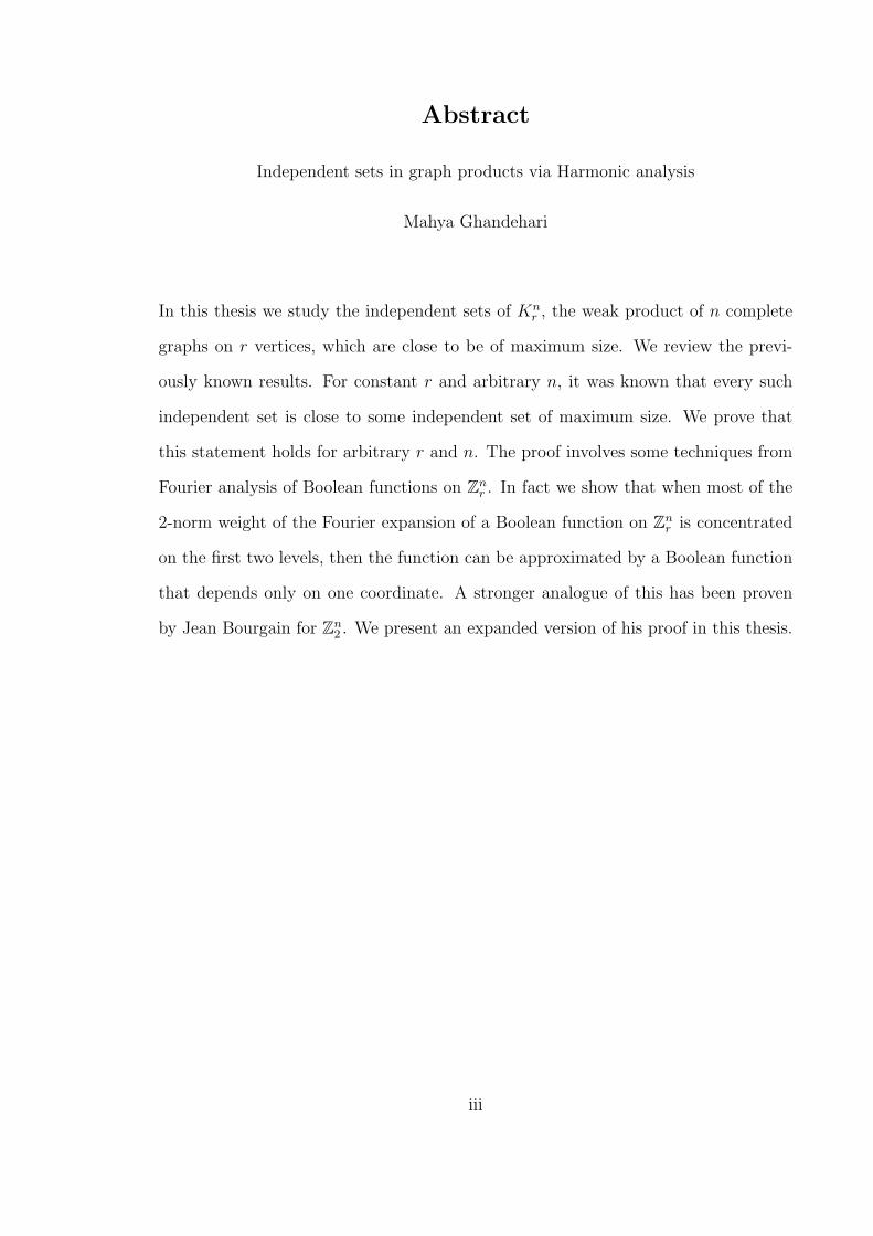
Abstract
Independent sets in graph products via Harmonic analysis
Mahya Ghandehari
In this thesis we study the independent sets of Knr , the weak product of n complete
graphs on r vertices, which are close to be of maximum size. We review the previ-
ously known results. For constant r and arbitrary n, it was known that every such
independent set is close to some independent set of maximum size. We prove that
this statement holds for arbitrary r and n. The proof involves some techniques from
Fourier analysis of Boolean functions on Znr . In fact we show that when most of the
2-norm weight of the Fourier expansion of a Boolean function on Znr is concentrated
on the first two levels, then the function can be approximated by a Boolean function
that depends only on one coordinate. A stronger analogue of this has been proven
by Jean Bourgain for Zn2 . We present an expanded version of his proof in this thesis.
iii
Acknowledgements
First and foremost, I would like to express my sincere gratitude to my supervisor,
Benoit Larose, who has supported me with his guidance, patience and encouragement.
I have greatly benefited from his valuable discussions and advises.
Many thanks to Vasek Chvatal and Galia Dafni for their helpful comments and
suggestions on the earlier version of this thesis. Also, I would like to thank the
staff and the faculty of the Department of Mathematics and Statistics at Concordia
University for providing such a nice academic environment.
I would like to thank Hamed Hatami for being a nice collaborator and a supportive
husband at the same time! He has always supported me with love, patience and
encouragement. The results of Chapter 4 is a joint work with him.
My two years of study at Concordia University have been one of the most won-
derful periods of my life. I am very grateful to my friends Aryan Bayani, Mona
Mehrandish and Amir Memartoluie who made my life in Montreal so much fun.
Finally, I would like to thank my family: my parents Mahboobeh and Mostafa
and my sisters Mahsa, Maryam and Mahta who always supported me with love and
encouraged me to learn. This thesis is dedicated to my family.
iv
Contents
1 Introduction 1
2 Background 8
2.1 Fourier analysis on Znr . . . . . . . . . . . . . . . . . . . . . . . . . . 8
2.2 Walsh expansion . . . . . . . . . . . . . . . . . . . . . . . . . . . . . 10
2.3 Some inequalities in Lp spaces . . . . . . . . . . . . . . . . . . . . . 12
2.4 Hyper-contractive inequalities . . . . . . . . . . . . . . . . . . . . . . 13
3 Stability of independent sets 17
3.1 Proof of Theorem 3.0.7 . . . . . . . . . . . . . . . . . . . . . . . . . . 18
3.2 Proofs of Lemmas 3.2.1 and 3.2.2 . . . . . . . . . . . . . . . . . . . . 23
4 Large independent sets 30
4.1 Introduction . . . . . . . . . . . . . . . . . . . . . . . . . . . . . . . 30
4.2 Main results . . . . . . . . . . . . . . . . . . . . . . . . . . . . . . . . 32
4.2.1 Proof of Lemma 4.2.1 . . . . . . . . . . . . . . . . . . . . . . 33
5 Fourier spectrum of Boolean functions 38
5.1 Fourier spectrum of Boolean functions . . . . . . . . . . . . . . . . . 38
6 Concluding remarks 51
Bibliography 53
v
Chapter 1
Introduction
In the paper “Graph products, Fourier analysis and spectral techniques” [1] Alon et.
al. considered the following interesting combinatorial problem: “Assume that at a
given road junction there are n three-position switches that control the red-yellow-
green position of the traffic light. You are told that whenever you change the position
of all the switches then the color of the light changes. Prove that in fact the light is
controlled by only one of the switches.”
The above problem can be viewed as the problem of finding all the possible types
of maximum independent sets in the product of complete graphs, which is studied in
the present thesis. In fact, the configuration space of the switches described above
can be simulated by the weak product of n copies of K3, the complete graph of size
3. Let us begin with some definitions.
Definition 1.0.1 Recall the following notations:
• Given a graph G, the vertex set of G is denoted by V (G), and the set of all
edges of G is denote by E(G).
• For a graph G, define |G| to be the number of vertices of G, i.e.
|G| = |V (G)|.
1
Chapter 1. Introduction 2
• For any two vertices u and v of G, by u ∼ v we mean that u and v are adjacent
in G.
Definition 1.0.2 A set I is an independent set of the graph G if:
• I ⊆ V (G).
• If x, y ∈ I then x y, i.e. no edge of G connects two vertices in I.
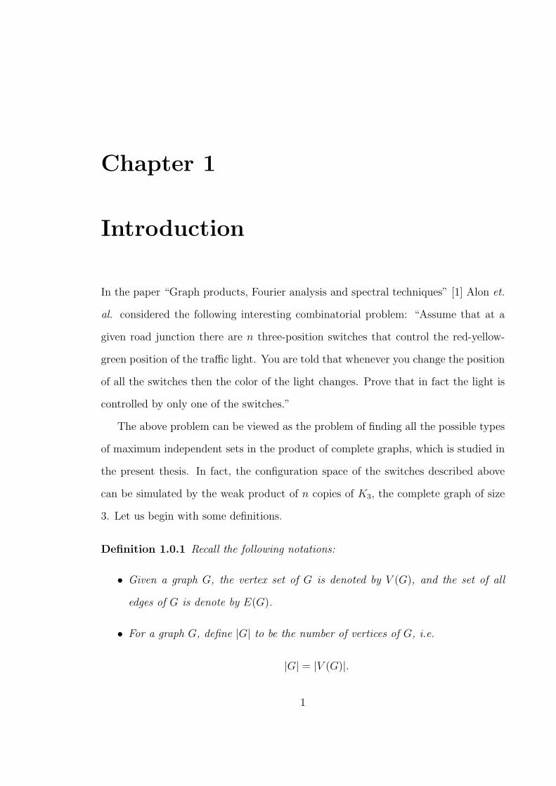
Example 1 The set I = 2, 4, 7 forms an independent set of the graph G shown
below.
x
h h
x x
h x
1
2
3
4 5
6
7
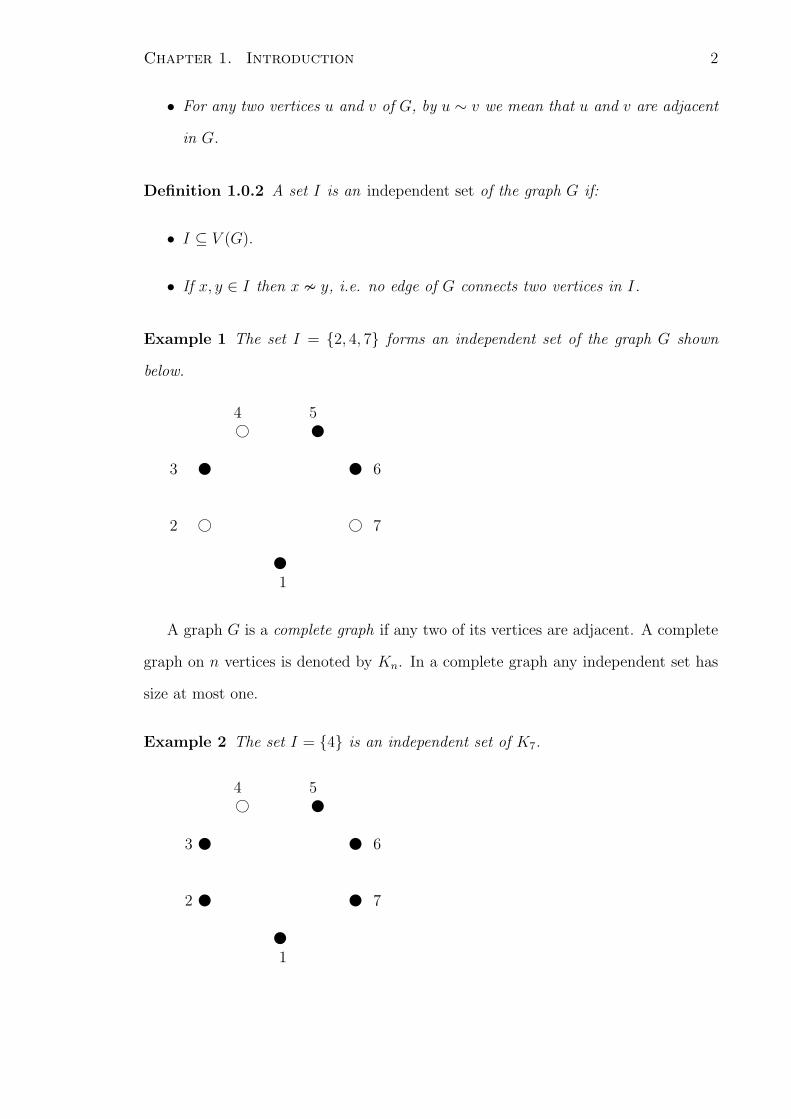
A graph G is a complete graph if any two of its vertices are adjacent. A complete
graph on n vertices is denoted by Kn. In a complete graph any independent set has
size at most one.
Example 2 The set I = 4 is an independent set of K7.
x
x x
x x
h x
1
2
3
4 5
6
7
Chapter 1. Introduction 3
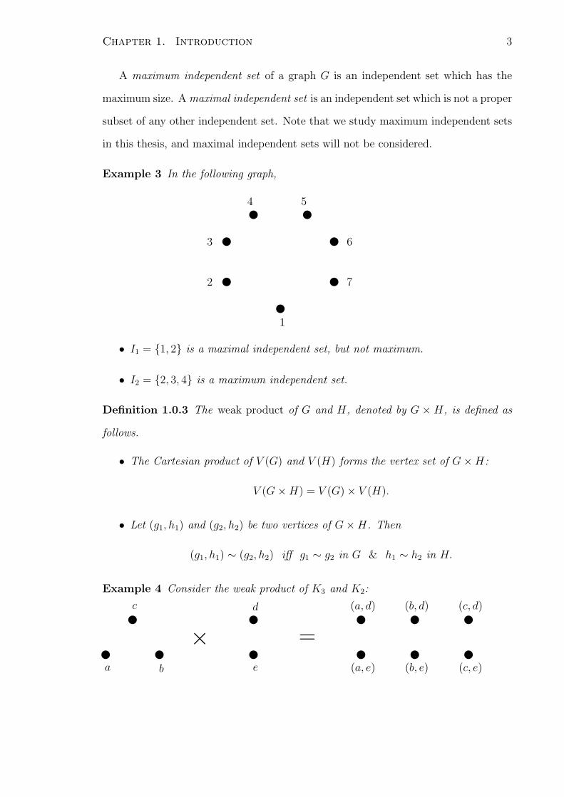
A maximum independent set of a graph G is an independent set which has the
maximum size. A maximal independent set is an independent set which is not a proper
subset of any other independent set. Note that we study maximum independent sets
in this thesis, and maximal independent sets will not be considered.
Example 3 In the following graph,
x
x x
x x
x x
1
2
3
4 5
6
7
• I1 = 1, 2 is a maximal independent set, but not maximum.
• I2 = 2, 3, 4 is a maximum independent set.
Definition 1.0.3 The weak product of G and H, denoted by G × H, is defined as
follows.
• The Cartesian product of V (G) and V (H) forms the vertex set of G×H:
V (G×H) = V (G)× V (H).
• Let (g1, h1) and (g2, h2) be two vertices of G×H. Then
(g1, h1) ∼ (g2, h2) iff g1 ∼ g2 in G & h1 ∼ h2 in H.
Example 4 Consider the weak product of K3 and K2:
x x
x
x
x
x x x
x x x
a b
c
×e
d
=
(a, d) (b, d) (c, d)
(a, e) (b, e) (c, e)
Chapter 1. Introduction 4
In this thesis we study the n-fold product of complete graphs on r > 2 vertices,
G = Knr = Kr ×Kr × . . .×Kr︸ ︷︷ ︸
n
.
Let r > 2 be an integer. We identify V (Kr) with Zr. It is then obvious that any two
vertices i and j of Kr are adjacent iff i 6= j. Now we can identify the vertices of G
with the elements of Znr in the natural way. By the definition of weak product, for
any two vertices (x1, . . . , xn) and (y1, . . . , yn) of G,
(x1, . . . , xn) ∼ (y1, . . . , yn) iff x1 6= y1, . . . , xn 6= yn.
Let 0 ≤ i ≤ r − 1 and 1 ≤ j ≤ n be two integers, and Iij be the set of all vertices
of G which have i in the j-th coordinate:
Iij = v ∈ Znr : vj = i.
Clearly, Iij is an example of a large independent set. Calculate the ratio of this
independent set, we have:
|Iij||G| =
rn−1
rn=
1
r.
It is easy to show that this is the maximum ratio that an independent set can attain,
and Iij is a maximum independent set of G (See [1]). In fact, for r > 2, these sets are
the only maximum independent sets of G, as Greenwell and Lovasz showed in [26].
Theorem 1.0.4 (See [1]) Let G = Knr , and assume r ≥ 3. Let I be an independent
set with |I| = |G|/r. Then there exists a coordinate i ∈ 1, . . . , n and k ∈ 0, . . . , r−1 such that
I = v : vi = k.
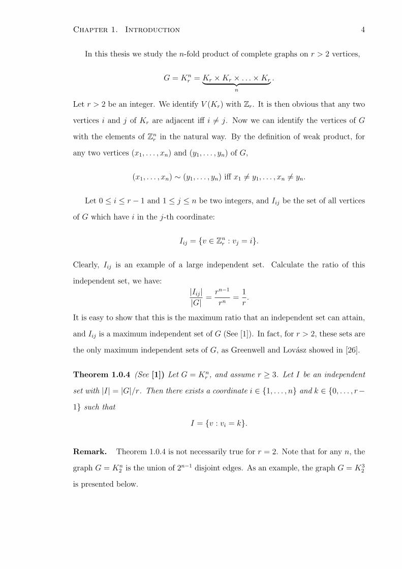
Remark. Theorem 1.0.4 is not necessarily true for r = 2. Note that for any n, the
graph G = Kn2 is the union of 2n−1 disjoint edges. As an example, the graph G = K3
2
is presented below.
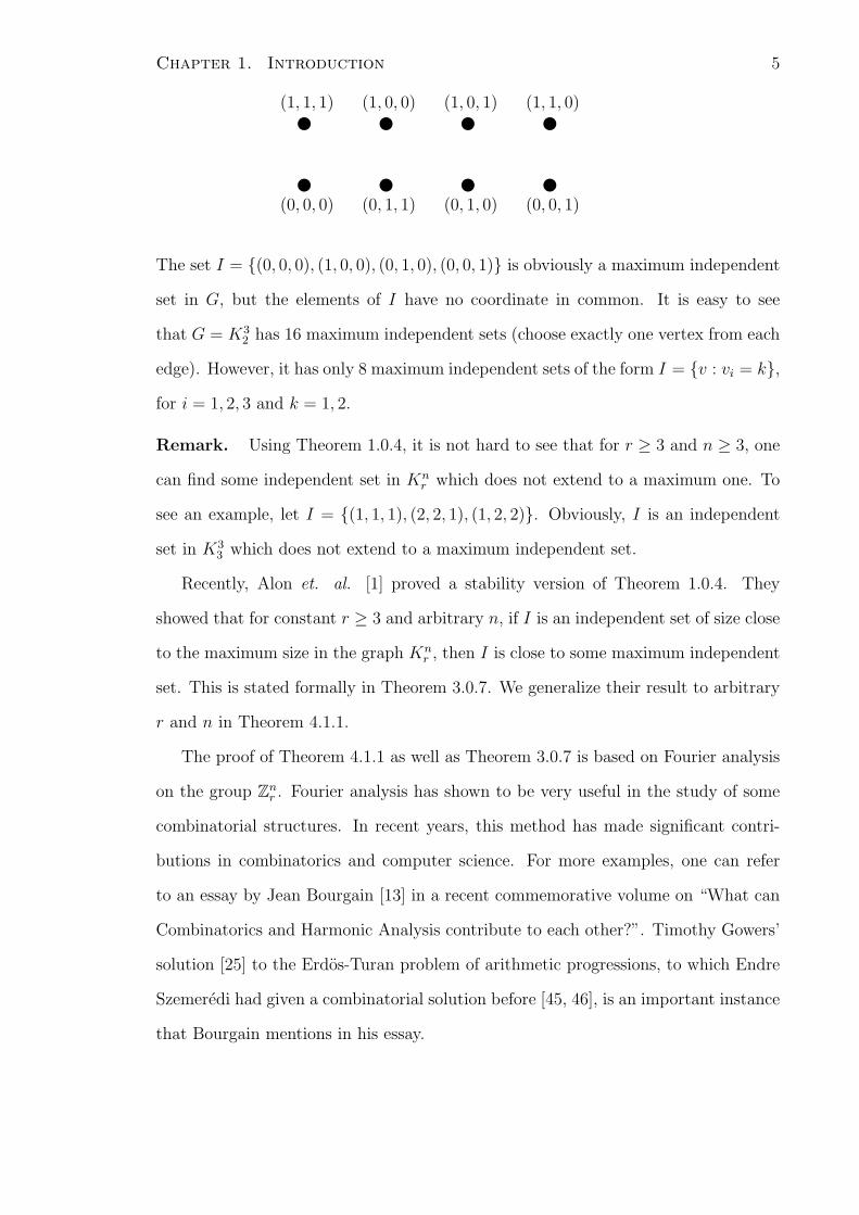
Chapter 1. Introduction 5
x x x x
x x x x
(0, 0, 0) (0, 1, 1) (0, 1, 0) (0, 0, 1)
(1, 1, 1) (1, 0, 0) (1, 0, 1) (1, 1, 0)
The set I = (0, 0, 0), (1, 0, 0), (0, 1, 0), (0, 0, 1) is obviously a maximum independent
set in G, but the elements of I have no coordinate in common. It is easy to see
that G = K32 has 16 maximum independent sets (choose exactly one vertex from each
edge). However, it has only 8 maximum independent sets of the form I = v : vi = k,for i = 1, 2, 3 and k = 1, 2.
Remark. Using Theorem 1.0.4, it is not hard to see that for r ≥ 3 and n ≥ 3, one
can find some independent set in Knr which does not extend to a maximum one. To
see an example, let I = (1, 1, 1), (2, 2, 1), (1, 2, 2). Obviously, I is an independent
set in K33 which does not extend to a maximum independent set.
Recently, Alon et. al. [1] proved a stability version of Theorem 1.0.4. They
showed that for constant r ≥ 3 and arbitrary n, if I is an independent set of size close
to the maximum size in the graph Knr , then I is close to some maximum independent
set. This is stated formally in Theorem 3.0.7. We generalize their result to arbitrary
r and n in Theorem 4.1.1.
The proof of Theorem 4.1.1 as well as Theorem 3.0.7 is based on Fourier analysis
on the group Znr . Fourier analysis has shown to be very useful in the study of some
combinatorial structures. In recent years, this method has made significant contri-
butions in combinatorics and computer science. For more examples, one can refer
to an essay by Jean Bourgain [13] in a recent commemorative volume on “What can
Combinatorics and Harmonic Analysis contribute to each other?”. Timothy Gowers’
solution [25] to the Erdos-Turan problem of arithmetic progressions, to which Endre
Szemeredi had given a combinatorial solution before [45, 46], is an important instance
that Bourgain mentions in his essay.
Chapter 1. Introduction 6
These methods are also playing an increasing role is the study of Boolean func-
tions which began with Kahn, Kalai, and Linial’s paper “The Influence of Variables on
Boolean Functions” [29]. This topic is significantly important in theoretical computer
science as well as economics (e.g., social choice) and statistical physics (e.g., percola-
tion, spin glasses). One can refer to [1, 2, 3, 5, 8, 14, 20, 23, 29, 34, 36, 38, 48, 39] to
see some examples.
Friedgut’s [20] proof for the long lasting open problem of the existence of a sharp
threshold for certain properties of random graphs is also based on Fourier analysis.
Recently many interesting nonembeddability results have been proven based on
Fourier analysis on 0, 1n and Rn. Indeed, the proofs of results in [17, 43, 41, 33,
37, 32] all have Fourier analytic components.
Finally we should mention its significant role in the theory of lower bounds in
approximation algorithms, especially in the near optimal inapproximability results of
Johan Hastad [27].
Perhaps one reason for the effectiveness of Fourier methods in combinatorics is
a general philosophy mentioned by Bourgain in [14] which claims that if f defines
a property of “high complexity”, then the support of its Fourier expansion has to
be “spread out”. Taking f to be the characteristic function of a combinatorial set
enables us to use this rule of thumb to study combinatorial objects. Lemma 4.2.1,
which we prove in Chapter 4, supports this philosophy.
This thesis is organized as follows. In Chapter 2 we review the basics of Fourier
analysis on Abelian groups. Some useful inequalities in Lp spaces have been stated.
We finish the chapter by a brief discussion on hyper-contractive inequalities. Chap-
ter 3 reviews the proof in [1] for the stability version of Theorem 1.0.4 (Theorem
3.0.7). Chapter 4 contains our new results which generalize Theorem 3.0.7. Chap-
ter 5 provides an expanded version of a paper of Jean Bourgain [14] where he proved
a very strong analogue of Lemma 4.2.1 for Zn2 . Finally Chapter 6 contains concluding

Chapter 1. Introduction 7
remarks and a discussion about open problems and some ideas about future work.
Chapter 2
Background
In this chapter we describe the necessary background. We also introduce some nota-
tions and provide some tools for the following chapters.
Sections 2.1 and 2.2 review the basics of Fourier analysis on Abelian groups.
Section 2.3 contains some useful inequalities in Lp spaces. Section 2.4 is devoted to
a brief discussion on hyper-contractive inequalities which play a crucial role in the
proofs presented in this thesis.
2.1 Fourier analysis on Znr
Let r > 2 and G = 0, 1, . . . , r − 1n = Znr . For any S ∈ G, let |S| = |i : Si 6= 0|
denote the number of nonzero coordinates of S. Let 0 = (0, 0, . . . , 0), and for each
1 ≤ i ≤ n let ei = (0, . . . , 1, . . . , 0) be the unit vector with 1 at the i-th coordinate
and zero everywhere else. For 0 ≤ k ≤ n, we define the “k-th level” of 0, . . . , r− 1n
to be the set of all S such that |S| = k.
Obviously G is an Abelian group. However, we can also think of G as a probability
space equipped with the uniform (product) measure µ, i.e. µ(S) = 1|G| for every S ∈ G.
Let f, g : G → C. We then define:
8
Chapter 2. Background 9
• ∫G
f(x)dx =∑
x∈G f(x)µ(x) = 1|G|
∑x∈G f(x).
• 〈f, g〉 = 1|G|
∑x∈G f(x)g(x).
• ‖f‖p =(∫
G|f(x)|pdx
) 1p .
Let us now find an orthonormal basis for the space of all complex-valued functions
on G. For any S ∈ G, we define uS : G → C to be
uS(T ) = e2πi〈S,T 〉
r ,
where T ∈ G and 〈S, T 〉 =∑n
i=1 SiTi (mod r).
The functions uS are called characters of G. The following properties of characters
are well-known and easy to prove.
• The set of characters forms a group under the operation of pointwise multipli-
cation.
• The mapping S 7→ uS is a homomorphism from G to the group of characters.
Since for any R ∈ G, we have:
(uSuT )(R) = uS(R)uT (R) = e2πi〈S,R〉
r e2πi〈T,R〉
r = e2πi〈S+T,R〉
r = uS+T (R),
and
u−T (R) = e2πi〈−T,R〉
r = e−2πi〈T,R〉
r = (u−1T )(R) = uT (R).
• Recall that the sum of the roots of unity is 0. So we have:
1.∑
T∈G uS(T ) = 0, for S 6= 0.
2. 1|G|
∑T∈G u0(T ) = 1, since u0 ≡ 1.
• The set of characters is an orthonormal basis:
1. 〈uS, uT 〉 = 0 if S 6= T.
Chapter 2. Background 10
2. 〈uS, uS〉 = 1.
• uS(T ) is a function of Ti : Si 6= 0.
As stated above, the set of all functions uS forms an orthonormal basis for the
space of all functions f : G → C. Therefore any such f has a unique expansion of
the form f =∑
S∈G f(S)uS, where
f(S) = 〈f, uS〉 =1
|G|∑T∈G
f(T )uS(T ).
From orthogonality it can be easily seen that
‖f‖22 =
∑S∈G
|f(S)|2, (2.1)
and
〈f, g〉 =∑S∈G
f(S)g(S),
where the first equality is referred to as Parseval’s identity. Let f>k =∑
|S|>k f(S)uS
(similarly f<k =∑
|S|<k f(S)uS) and f=k =∑
|S|=k f(S)uS. We occasionally refer to
f=k as the k-th level of Fourier expansion of f . Note that for any function f , f(0) is
the expectation of f , and ‖f≥1‖22 is the variance of f .
2.2 Walsh expansion
Denote 1, 2, . . . , n by [n].
Definition 2.2.1 (Biased Walsh-Products). Let 0 < p < 1. For every i ∈ [n],
we define the i-th p-biased Rademacher function ri : P([n]) → R by
ri(x) =
√p
1−pi /∈ x
−√
1−pp
i ∈ x
For every set ∅ 6= S ⊆ [n], its corresponding p-biased Walsh-product is defined by
rS =∏i∈S
ri.
Also let r∅ = 1.
Chapter 2. Background 11
Note that every element of P([n]) can be identified with a vector in Zn2 in the
natural way. So we can restate Definition 2.2.1 as the following. Let 0 < p < 1. For
every i ∈ [n], we define the i-th p-biased Rademacher function ri : Zn2 → R by
ri(X) =
√p
1−pXi = 0
−√
1−pp
Xi = 1
for every X = (X1, . . . , Xn) ∈ Zn2 .
The corresponding p-biased Walsh-product of S, S = (S1, . . . , Sn) ∈ Zn2 , is now
defined by
rS =∏Si=1
ri.
Let µ be the p-biased measure on Zn2 , which is defined as:
µ(T ) = p|T |(1− p)n−|T |,
for any T ∈ Zn2 , i.e. every coordinate of T is 1 with probability p, and is 0 with
probability 1− p. We also define the integration with respect to the measure µ:
∫
Zn2
fdµ(S) =∑
S∈Zn2
f(S)µ(S).
It is easy to see that the set of the p-biased Walsh-products forms an orthonormal
basis for L2(Zn2 , dµ), the L2-space of all real valued functions on Zn
2 with
‖f‖22 =
∫
Zn2
|f |2dµ =∑
S∈Zn2
|f(S)|2µ(S).
Therefore any function f : Zn2 → R can be written as a linear combination f =
∑S∈Zn
2f(S)rS, called the Walsh expansion of f , where
f(S) = 〈f, rS〉 =
∫
Zn2
f(x)rS(x)dµ(x).
If p = 12, using the above argument, we get an orthonormal basis for the space of all
functions f : Zn2 → R with the uniform measure.
Chapter 2. Background 12
2.3 Some inequalities in Lp spaces
In this section we list a few elementary inequalities in Lp spaces.
Theorem 2.3.1 (Holder) If p and q are nonnegative extended real numbers (i.e.
p, q ∈ R≥0 ∪ ∞) such that 1p
+ 1q
= 1, and if f ∈ Lp and g ∈ Lq, then fg ∈ L1 and
∫|fg| ≤ ‖f‖p‖g‖q.
Corollary 2.3.2 Let p, q, r ≥ 1 and 0 < θ < 1 be such that 1q
= θp
+ 1−θr
. Then for
each h ∈ Lp ∩ Lr we have
‖h‖q ≤ ‖h‖θp‖h‖1−θ
r .
Proof. Let p1 = pqθ
and q1 = rq(1−θ)
, so we have 1p1
+ 1q1
= 1. Using Holder inequality
for f = hqθ and g = hq(1−θ) we have:
∫(|h|qθ)(|h|q(1−θ)) ≤
(∫(|h|qθ)
pθq
) qθp
(∫(|h|q(1−θ))
rq(1−θ)
) q(1−θ)r
.
Hence ∫|h|q ≤
((
∫|h|p)1/p
)qθ ((
∫|h|r)1/r
)q(1−θ)
.
Therefore we have:
(∫|h|q
)1/q
≤(∫
|h|p)θ/p (∫
|h|r) 1−θ
r
.
The next theorem is also known as generalized Minkowski inequality. One can
refer to [28] to see the proof.
Theorem 2.3.3 (See [28]) Let (M1,M1, µ1) and (M2,M2, µ2) be two σ-finite mea-
sure spaces. If f is a measurable function on M1 ×M2 and 0 < q ≤ r ≤ ∞, then
‖‖f‖Lq(M1,dµ1)‖Lr(M2,dµ2) ≤ ‖‖f‖Lr(M2,dµ2)‖Lq(M1,dµ1).
Chapter 2. Background 13
2.4 Hyper-contractive inequalities
Let Zn2 be the probability space equipped with the p-biased measure. Recall that the
Bonami-Beckner operator Tρ, 0 ≤ ρ ≤ 1, is a linear operator on the space of functions
Zn2 → R defined by
Tρ[f ](x) = E[f(y)],
where y is a ρ-correlated copy of x, i.e. at each point x, Tρ[f ](x) is the expected value
of f when a (1 − ρ)-fraction of the coordinates in x are randomly re-assigned (we
say that a (1 − ρ)-noise is applied to x). This is equivalent to saying that Tρ[f ](x),
at each point x, is the expected value of f when each coordinate is chosen with the
probability 1− ρ, and the chosen coordinate is randomly re-assigned.
Now let f : Zn2 → R be a function, and consider its Walsh expansion f =
∑S∈Zn
2f(S)rS. Obviously Tρ is a linear operator since expectation is linear. There-
fore,
Tρ[f ] = Tρ[∑
S∈Zn2
f(S)rS] =∑
S∈Zn2
f(S)Tρ[rS].
Hence it only remains to evaluate Tρ on the biased Walsh-products, as shown in the
following lemma.
Lemma 2.4.1 Tρ[rS] = ρ|S|rS
Proof. Let us first consider the case where |S| = 1. Without loss of generality we
can assume that rS = r1. Let X ∈ Zn2 such that X1 = 0. Thus r1(X) =
√p
1−p. Now
using the definition of Tρ, we get:
Tρ[rS] = ρ
√p
1− p+ (1− ρ)p(−
√1− p
p) + (1− ρ)(1− p)
√p
1− p= ρ
√p
1− p.
Using the same argument for X ∈ Zn2 with X1 = 1, we conclude that Tρ[rS] = ρrS
when |S| = 1. It is also easy to see that Tρ[rS] =∏
Si=1 Tρ[ri] since ri and rj are
independent when i 6= j. Therefore
Tρ[rS] =∏Si=1
ρri = ρ|S|rS.
Chapter 2. Background 14
Recall that f : Zn2 → R is a function with the Walsh expansion f =
∑S∈Zn
2f(S)rS.
Now using Lemma 2.4.1, we have:
Tρ[f ] =∑
S∈Zn2
ρ|S|f(S)rS. (2.2)
Using Lemma 5 of [12], it can be easily proved that this operator is contractive with
respect to any p-norm, p ≥ 1. However, the Bonami-Beckner inequality is powerful
since it shows that this operator remains contractive from Lp to Lq for certain values
of p and q with q > p. This is the reason it is often referred to as a hyper-contractive
inequality. The inequality was originally proved by Bonami in 1970 [9] and then
independently by Beckner in 1973 [6]. It was first used to analyze discrete problems
in a paper by Kahn, Kalai and Linial [29] where they considered the influence of
variables on Boolean functions. The inequality is also very important in the study of
combinatorics of 0, 1n [15, 16, 20], percolation and random graphs [47, 22, 8, 21]
and many other applications [7, 2, 44, 4, 19, 31, 42].
Theorem 2.4.2 (Bonami-Beckner) Let Zn2 be a measure space endowed with the
uniform measure. Let f : Zn2 → R and q ≥ p ≥ 1. Then
‖Tρf‖q ≤ ‖f‖p for all 0 ≤ ρ ≤ (p−1)1/2
(q−1)1/2 .
The dual version of Theorem 2.4.2 can be formulated as Theorem 2.4.3. The first
part of this theorem has been presented in Lemma 2.1 of [1].
Theorem 2.4.3 Let f : Zn2 → R be a function that is a linear combination of the
uT : |T | ≤ k. Then for p ≥ 2,
‖f‖p ≤ (√
p− 1)k‖f‖2;
and for 1 ≤ p ≤ 2,
‖f‖p ≥ (√
p− 1)k‖f‖2.
Chapter 2. Background 15
Proof. First assume that p ≥ 2. By Theorem 2.4.2, assuming ρ =√
1p−1
we have
‖Tρ[f ]‖p ≤ ‖f‖2. Note that for every T ∈ Zn2 ,
uT (S) = e2πi2〈S,T 〉 = (−1)〈S,T 〉 = rT (S),
holds for every S ∈ Zn2 . Therefore uT = rT in the case of the uniform measure on Zn
2 .
Thus since f is a linear combination of the uT : |T | ≤ k and ρ ≤ 1, by (2.2) we
have ‖Tρ[f ]‖p ≥ ρk‖f‖p. So we have:
ρk‖f‖p ≤ ‖f‖2
which yields the claim.
For the case 1 ≤ p ≤ 2, the same argument with ρ =√
p− 1 implies the claim.
Theorem 2.4.3 tells us that if a function f is a linear combination of the uT : |T | ≤k, then all the p-norms (p ≥ 1) of f are equivalent up to constants depending only on
p and k and not on the function. This can even be generalized to 0 < p < 1. However
these should not be called norms since they do not satisfy the triangle inequality.
Theorem 2.4.4 Let f : Zn2 → R≥0 be a function that is a linear combination of the
uT : |T | ≤ k. Then for p ≤ 1,
‖f‖p ≥ (3− p)−k(4−p)
2p ‖f‖2.
Proof. Fix some p1 > 1. By applying the Holder inequality (Lemma 2.3.1) to
f 2 = fp
p1 f2− p
p1 , we have
∫f 2 ≤
(∫|f |p
) 1p1
(∫|f |
2p1−pp1−1
)P1−1p1
. (2.3)
Since 2p1−pp1−1
> 2, by Theorem 2.4.3
(∫|f |(
2p1−pp1−1
)
) P1−12p1−p
≤(
2p1 − p
p1 − 1− 1
) k2
‖f‖2. (2.4)
Chapter 2. Background 16
Combining (2.3) and (2.4) we get
(p1 − p + 1
p1 − 1
)− k(2p1−p)2p1 ‖f‖2− 2p1−p
p12 ≤
(∫|f |p
) 1p1
,
or (p1 − p + 1
p1 − 1
)− k(2p1−p)2p
‖f‖2 ≤ ‖f‖p.
Substituting p1 = 2 implies the result.
The Bonami-Beckner inequality admits a reversed form which was first proved by
Christer Borell [10] in 1982. The reversed form studies the case where q ≤ p ≤ 1,
while the norms in the original inequality are all at least 1. We refer the reader to
[40] for a proof of Theorem 2.4.5.
Theorem 2.4.5 (Reverse Bonami-Beckner) Let f : Zn2 → R≥0 and q ≤ p ≤ 1.
Then
‖Tρf‖q ≥ ‖f‖p for all 0 ≤ ρ ≤ (1−p)1/2
(1−q)1/2 .
There are different generalizations of Theorem 2.4.2. We finish this chapter with
stating a version dealing with functions on Znr , which has been proved in [1].
Theorem 2.4.6 [1] For every r ≥ 2 there exists C > 0 such that the following holds.
Let G = Znr be a probability space equipped with the uniform measure, and f : G → C
be a function whose Fourier expansion is concentrated on the first k + 1 levels, that
is, f is a linear combination of the uT : |T | ≤ k. Then
‖f‖4 ≤ Ck‖f‖2.
Chapter 3
Stability of independent sets
In this chapter we present some results concerning the maximum or nearly maximum
independent sets of G = Knr . The results and proofs presented here are from a paper
by Alon et. al. [1].
As stated in Theorem 1.0.4, the sets Iij = x ∈ Znr : xi = j, for 1 ≤ i ≤ n and
0 ≤ j ≤ r − 1, are the only maximum independent sets of Knr for r ≥ 3. A stability
version of Theorem 1.0.4 has been proved in [1]:
Theorem 3.0.7 [1] For every r ≥ 3, there exists a constant M = M(r) such that
for any ε > 0 the following is true. Let G = Knr and J be an independent set of G
such that |J ||G| = 1
r(1 − ε). Then there exists an independent set I with |I|
|G| = 1r
such
that |J4I||G| < Mε
r.
In Theorem 3.0.7, “4” denotes the symmetric difference. Theorem 3.0.7 asserts
that any independent set J of G which is close to be of maximum size is close to some
set Iij, i.e. J is close to being determined by one vertex.
The proof of Theorem 3.0.7 uses some Fourier analysis methods. We present this
proof in Section 3.1. There are a few lemmas regarding Boolean functions on Znr
which are the key lemmas in the proof of the theorem. In Section 3.2 we review the
proofs of these lemmas.
17
Chapter 3. Stability of independent sets 18
3.1 Proof of Theorem 3.0.7
Let r ≥ 3 be an integer and G = Knr . We identify the vertices of G with the elements
of Znr as shown in Chapter 1. Throughout this chapter, we think of Zn
r as a probability
space with the uniform product measure, denoted by µ, i.e.
µ(S) =1
|G| for every S ∈ G.
Let I be an independent set in G. Let f be the characteristic function of I, i.e. f
is a Boolean function on Znr such that
f(x) =
1 x ∈ I
0 x /∈ I
The function f has the following properties:
• α = |I||G| =
∫G
f(x)dx = f(0).
• α = ‖f‖22 =
∑S∈Zn
r|f(S)|2.
• ∑S∈Zn
r|f(S)|2 ( −1
r−1
)|S|= 0.
Where α is defined to be the ratio of I, α = µ(I) = |I||G| . The first equality is obvious.
The second one can be easily shown using Parseval’s identity. We will later present
the proof of the third equality in Lemma 3.1.1. Assuming these facts, we get:
∑
S 6=0
|f(S)|2 = α− α2. (3.1)
∑
S 6=0
|f(S)|2( −1
r − 1
)|S|= −α2. (3.2)
Now we get valuable information on the Fourier expansion of f using (3.1) and
(3.2). We consider the following distribution to interpret this information. Let T be
a random variable which takes values in G\0 with
Pr[T = S] =|f(S)|2α− α2
.
Chapter 3. Stability of independent sets 19
Let
X = X(T ) =
( −1
r − 1
)|T |.
Calculating E(X) and using (3.2), we have
E(X) =∑
S 6=0
( −1
r − 1
)|S| |f(S)|2α− α2
=−α2
α− α2=
−α
1− α.
It is important to note that for all T , X(T ) ≥ −1r−1
. Also equality X(T ) = −1r−1
holds
if and only if |T | = 1. We now break our analysis into three cases: α > 1/r, α = 1/r
and α = 1−εr
. A simple argument shows that the first case cannot happen. One can
then use Lemmas 3.2.1 and 3.2.2, discussed in Section 3.2, to analyze the second and
third cases.
Case 1:
Let α > 1/r. Since −x1−x
is a decreasing function, we have E(X) = −α1−α
< −1r−1
.
However, note that E(X) ≥ −1r−1
since X(T ) ≥ −1r−1
for all T . Therefore the assump-
tion α > 1/r yields a contradiction. Hence if I is an independent set then µ(I) ≤ 1/r.
Case 2:
Let α = 1/r. Then E(X) = −α1−α
= −1r−1
. Moreover, since X(T ) ≥ −1r−1
for all T ,
E(X) = −1r−1
implies that X ≡ −1r−1
. Now recalling X(T ) = −1r−1
iff |T | = 1, we
conclude that for all S of size bigger than one, the following holds:
Pr[T = S] =|f(S)|2α− α2
= 0.
Hence f(S) = 0 for all S of size bigger than one. Therefore f has all its Fourier
expansion concentrated on the first two levels, which implies that f is constant or
depends only on one coordinate (see Lemma 3.2.1). Obviously f is not a constant
function, because it is the characteristic function of an independent set. Therefore it
depends only on one coordinate, and it must be the characteristic function of Iij for
Chapter 3. Stability of independent sets 20
some i and j. Thus we have just given another proof for Theorem 1.0.4.
Case 3:
Finally we consider the case α = 1−εr
, where α is slightly less than 1/r. We then have
E(X) =−1 + ε
r − 1 + ε>
−1
r − 1.
So E(X) is very close to −1r−1
, its minimal value, from which we will conclude that
most of the Fourier expansion of f is concentrated on the first two levels.
Recall that for all S of size bigger than one, we have
X(S) ≥ −1
(r − 1)3>
−1
r − 1. (3.3)
Now let Y = Y (T ) = X(T ) + 1r−1
. It is easy to verify the following properties of Y :
1. Y ≥ 0.
2. E(Y ) = E(X) + 1r−1
= −1+εr−1+ε
+ 1r−1
= εr(r−1)(ε+r−1)
.
3. Y (T ) > 0 iff X(T ) > −1r−1
iff |T | > 1.
4. If Y > 0 then Y ≥ −1(r−1)3
+ 1r−1
= r(r−2)(r−1)3
.
Now by Markov’s inequality, we get
Pr[Y > 0] ≤ E(Y )(r − 1)3
r(r − 2). (3.4)
Using (3.4) and the second property of Y together with r ≥ 3, we have
Pr[Y > 0] ≤ ε
ε + r − 1· (r − 1)2
r − 2≤ 2ε. (3.5)
The conclusion of (3.5) is that for each ε > 0 and for every independent set I with
α = µ(I) = 1−εr
we have
∑
|S|>1
|f(S)|2 = (α− α2)∑
|S|>1
Pr[T = S] = (α− α2)Pr[Y > 0] ≤ 1
r(2ε) ≤ 2ε
r,
Chapter 3. Stability of independent sets 21
where f is the characteristic function of I.
We have just shown that most of the Fourier expansion of f is concentrated on
the first two levels. Now we deduce Theorem 3.0.7 from Lemma 3.2.2, which says
that there exists some Boolean function g that depends on at most one coordinate
such that
‖f − g‖22 <
(2K)(2ε)
(α− α2 − 2εr)(r)
<Mε
r,
where M is a function of r. Note that we assume ε to satisfy ‖f‖22− (2K)(2ε)
(α−α2− 2εr
)(r)> 0.
This assumption disallows the uninteresting cases, since if ε is not small enough then
g ≡ 0 is also a possibility.
We now continue with the proof of Lemma 3.1.1, which has been used in proving
Theorem 3.0.7.
Lemma 3.1.1 [1] Let I ⊂ Znr be an independent set in G, and let f : Zn
r → 0, 1be its characteristic function, i.e. f(x) = 1 iff x ∈ I. Then,
∑
S∈Znr
|f(S)|2( −1
r − 1
)|S|= 0.
Proof. First define D = (Zr\0)n and d = |D|. It is then obvious that two vertices
u, v ∈ Znr are adjacent iff u− v ∈ D. Now define
• fτ (x) = f(x + τ) for any τ ∈ D.
• A(f) = 1d
∑τ∈D fτ .
Note that A(f) acts as an averaging operator which replaces f(x) by the average of
f on the neighbors of x. We now need to prove the following claims:
Claim 3.1.2 〈f, A(f)〉 = 0.
Proof. Let x ∈ Znr . Recall that for any τ ∈ D, x and x + τ are adjacent in G. So
for every x ∈ Znr , since I is an independent set, we have:
fτ (x)f(x) = 0.
Chapter 3. Stability of independent sets 22
Therefore
〈f, fτ 〉 = 0. (3.6)
Recalling the definition of A(f), we have:
〈f, A(f)〉 = 〈f,1
d
∑τ∈D
fτ 〉 =1
d
∑τ∈D
〈f, fτ 〉 = 0.
Now we compute the Fourier coefficients of fτ and A(f) in terms of the Fourier
coefficients of f .
Claim 3.1.3 fτ (S) = f(S)uτ (S).
Proof. Using the definition of the Fourier expansion of fτ , we have:
fτ (S) =
∫fτ (x)uS(x)dx =
∫f(x + τ)uS(x)dx
=
∫f(x)uS(x− τ)dx =
∫f(x)uS(x)uS(−τ)dx
=
∫f(x)uS(x)uS(τ)dx = f(S)uτ (S).
Claim 3.1.4 A(f)(S) = f(S)( −1
r−1
)|S|.
Proof. Let ω = e2πi/r. Recall that D = (Zr\0)n and d = |D| = (r − 1)n. By
Claim 3.1.3,
A(f)(S) =
(1
d
∑τ∈D
fτ )(S) =1
d
∑τ∈D
fτ (S) =1
df(S)
∑τ∈D
uτ (S).
We also have
∑τ∈D
uτ (S) =n∏
j=1
r−1∑
k=1
ωkSj =∏
j:Sj=0
(r − 1)∏
j:Sj 6=0
(−1),
since the sum of the roots of unity is 0. Finally we get:
A(f)(S) =1
(r − 1)nf(S)(r − 1)n−|S|(−1)|S| = f(S)
( −1
r − 1
)|S|,
Chapter 3. Stability of independent sets 23
which completes the proof of Claim 3.1.4.
Back to the proof of Lemma 3.1.1, we can now use Claim 3.1.4 and Claim 3.1.2,
and we have
0 = 〈f,A(f)〉 =∑
S∈Znr
f(S)A(f)(S) =∑
S∈Znr
|f(S)|2( −1
r − 1
)|S|.
3.2 Proofs of Lemmas 3.2.1 and 3.2.2
In this section we prove some lemmas which have been used in the proof of Theorem
3.0.7 in Section 3.1.
Lemma 3.2.1 [1] Let f : Znr → 0, 1 be such that all its Fourier expansion is
concentrated on the first two levels:
|S| > 1 ⇒ f(S) = 0.
Then f is either constant or depends on precisely one coordinate.
Proof. The Fourier expansion of f is concentrated on the first two levels, therefore
f is of the form f = f(0) +∑
T :|T |=1 f(T ). Denoting a0 = f(0), the function f can
be written as
f(S) = a0 +n∑
j=1
r−1∑
k=1
aj,ke2πisjk
r .
Moreover f = f 2, since f is a Boolean function. Let us now compare the coefficients
of e2πiSj1
k
r e2πiSj2
l
r in f and f 2. If j1 6= j2 then the coefficients of e2πiSj1
k
r e2πiSj2
l
r in f and
f 2 are 0 and 2aj1,kaj2,l respectively, and by the uniqueness of the Fourier expansion,
we get
aj1,kaj2,l = 0 whenever j1 6= j2.
Chapter 3. Stability of independent sets 24
It is now obvious that there exists one coordinate, say jl, such that for all k and j,
j 6= jl, we have aj,k = 0. Therefore f is of the form
f(S) = a0 +r−1∑
k=1
ake2πiSlk
r .
Lemma 3.2.2 [1] Let r ≥ 2 and let C = C(r) be the constant from Theorem 2.4.6.
Let K = 2 + 32C8. Then for any ε > 0 the following holds. Let f : Znr → 0, 1 be a
function such that Pr[f = 1] = α and furthermore assume that
∑
|S|>1
|f(S)|2 = ε.
Then there exists a Boolean function g : Znr → 0, 1 which depends on at most one
coordinate such that
‖f − g‖22 ≤
2K
α− α2 − εε.
Remark. Note that f is a Boolean function, and we assume that Znr is a probability
space endowed with the uniform measure. Therefore we have
α = Pr[f = 1] =
∫
Znr
f(S)dS = f(0),
and
α =
∫
Znr
f(S)dS =
∫
Znr
|f(S)|2dS = ‖f‖22.
Hence
α− α2 − ε = ‖f‖22 − |f(0)|2 −
∑
|S|>1
|f(S)|2 =∑
|S|=1
|f(S)|2,
which implies that ε ≤ α− α2.
Remark. In the above theorem, we can assume that ε ≤ 14C8 , where C is the
constant from Theorem 2.4.6. Note that if ε > 14C8 then taking K = 2 + 32C8 leads
Chapter 3. Stability of independent sets 25
to a trivial Kε-approximation of f . This is because Kε > 1 and for any function
g : Znr → 0, 1, obviously ‖f − g‖2
2 ≤ 1.
Proof of Lemma 3.2.2. Let fS =∑
|T |≤1 f(T )uT and fL =∑
|T |>1 f(T )uT , where
S represents small and L stands for large.
The lemma is trivial when fS is assumed to be a Boolean function. Indeed, if fS
is Boolean then it depends on at most one coordinate by Lemma 3.2.1. Hence we can
take g to be fS and we are done. To prove the lemma in the general case, we will
first show that fS is close to being Boolean. We can then easily conclude the desired
result.
Define h = f 2S − fS. It is obvious that h = 0 iff fS is Boolean. Thus we can
consider h as a measure that determines how far fS is from being Boolean. In order
to show that fS is close to being Boolean, we will prove that the 2-norm of h is small,
as stated in the following lemma.
Lemma 3.2.3 [1] Let C be the constant from Theorem 2.4.6 and let λ = 32C8. Then
E(|h|2) ≤ λε,
where∑
|S|>1 |f(S)|2 = ε and ε ≤ 14C8 .
We postpone the proof of Lemma 3.2.3, and present its important corollary first.
Corollary 3.2.4 [1] There exists 1 ≤ j ≤ n such that for the function g′, defined as
g′(x) = f(0) +r−1∑
k=1
f(kej)e2πikxj
r , (3.7)
it is true that ‖g′ − f‖22 ≤ ε
(1 + λ
2(α−α2−ε)
).
Assuming Corollary 3.2.4, Lemma 3.2.2 can be easily proven. Indeed, let majj[f ](y) :
Znr → 0, 1 be the function taking values of 0 or 1 according to the majority value of
Chapter 3. Stability of independent sets 26
f(x) over all x ∈ Znr : xj = yj. It is easy to see that if g : Zn
r → 0, 1 is a Boolean
function which depends only on the j-th coordinate, then
‖f −majj[f ]‖22 ≤ ‖f − g‖2
2. (3.8)
Let g′′ be the function obtained by rounding g′ to the nearest number in 0, 1. Hence
‖f − g′′‖22 ≤ 4‖f − g′‖2
2. (3.9)
Now using (3.8) and (3.9), we get:
‖f −majj[f ]‖22 ≤ 4‖f − g′‖2
2 ≤2K
α− α2 − εε,
which completes the proof of Lemma 3.2.2.
Now it only remains to prove Corollary 3.2.4 and Lemma 3.2.3. We will first
present the proof of the corollary assuming Lemma 3.2.3. We then finish the section
with the review of the proof of this lemma.
Proof of Corollary 3.2.4. Let g0 = f(0). For 1 ≤ i ≤ n, let gi =∑r−1
k=1 f(kei).
Recall that f = g0 + g1 + g2 + . . . + gn. Denote ai = ‖gi‖22 =
∑r−1k=1 |f(kei)|2. Without
loss of generality we can assume that ‖g1‖22 ≥ ‖g2‖2
2 ≥ . . . ≥ ‖gn‖22.
Let us first compute h(S) on the second level. Let i 6= j. Then, since f(S) is 0 on
the second level, we have:
h(k1ei + k2ej) = f 2S(k1ei + k2ej)− fS(k1ei + k2ej) = 2f(k1ei)f(k2ej). (3.10)
Since E(|h|2) = ‖h‖22 =
∑T∈Zn
r|h(T )|2, we can get a lower bound for E(|h|2) by
summing only over T ’s of the second level (i.e. T = k1ei + k2ej for i, j ∈ [n] with
Chapter 3. Stability of independent sets 27
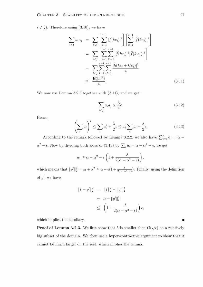
i 6= j). Therefore using (3.10), we have
∑i<j
aiaj =∑i<j
[r−1∑
k=1
|f(kei)|2][
r−1∑
k=1
|f(kej)|2]
=∑i<j
[r−1∑
k=1
r−1∑
k′=1
|f(kei)|2|f(k′ej)|2]
=∑i<j
r−1∑
k=1
r−1∑
k′=1
|h(kei + k′ej)|24
≤ E(|h|2)4
. (3.11)
We now use Lemma 3.2.3 together with (3.11), and we get:
∑i<j
aiaj ≤ λ
4ε. (3.12)
Hence, (∑i
ai
)2
≤∑
i
a2i +
λ
2ε ≤ a1
∑i
ai +λ
2ε. (3.13)
According to the remark followed by Lemma 3.2.2, we also have∑n
i=1 ai = α −α2 − ε. Now by dividing both sides of (3.13) by
∑i ai = α− α2 − ε, we get:
a1 ≥ α− α2 − ε
(1 +
λ
2(α− α2 − ε)
),
which means that ‖g′‖22 = a1 +α2 ≥ α− ε(1+ λ
2(α−α2−ε)). Finally, using the definition
of g′, we have:
‖f − g′‖22 = ‖f‖2
2 − ‖g′‖22
= α− ‖g′‖22
≤(
1 +λ
2(α− α2 − ε)
)ε,
which implies the corollary.
Proof of Lemma 3.2.3. We first show that h is smaller than O(√
ε) on a relatively
big subset of the domain. We then use a hyper-contractive argument to show that it
cannot be much larger on the rest, which implies the lemma.
Chapter 3. Stability of independent sets 28
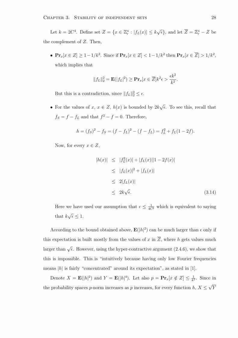
Let k = 2C4. Define set Z = x ∈ Znr : |fL(x)| ≤ k
√ε, and let Z = Zn
r − Z be
the complement of Z. Then,
• Prx[x ∈ Z] ≥ 1−1/k2. Since if Prx[x ∈ Z] < 1−1/k2 then Prx[x ∈ Z] > 1/k2,
which implies that
‖fL‖22 = E(|fL|2) ≥ Prx[x ∈ Z]k2ε >
εk2
k2.
But this is a contradiction, since ‖fL‖22 ≤ ε.
• For the values of x, x ∈ Z, h(x) is bounded by 2k√
ε. To see this, recall that
fS = f − fL and that f 2 − f = 0. Therefore,
h = (fS)2 − fS = (f − fL)2 − (f − fL) = f 2L + fL(1− 2f).
Now, for every x ∈ Z,
|h(x)| ≤ |f 2L(x)|+ |fL(x)||1− 2f(x)|
≤ |fL(x)|2 + |fL(x)|
≤ 2|fL(x)|
≤ 2k√
ε. (3.14)
Here we have used our assumption that ε ≤ 14C8 which is equivalent to saying
that k√
ε ≤ 1.
According to the bound obtained above, E(|h|2) can be much larger than ε only if
this expectation is built mostly from the values of x in Z, where h gets values much
larger than√
ε. However, using the hyper-contractive argument (2.4.6), we show that
this is impossible. This is “intuitively because having only low Fourier frequencies
means |h| is fairly “concentrated” around its expectation”, as stated in [1].
Denote X = E(|h|2) and Y = E(|h|4). Let also p = Prx[x /∈ Z] ≤ 1k2 . Since in
the probability spaces p-norm increases as p increases, for every function h, X ≤ √Y
Chapter 3. Stability of independent sets 29
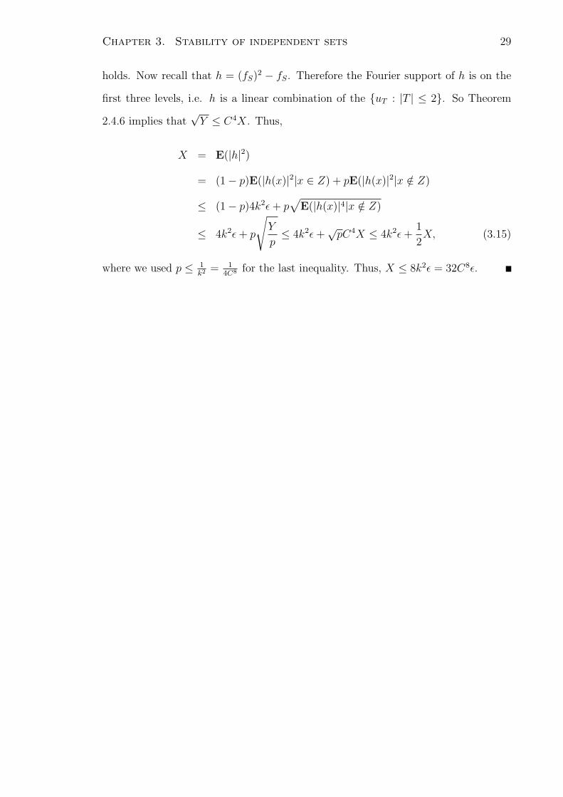
holds. Now recall that h = (fS)2 − fS. Therefore the Fourier support of h is on the
first three levels, i.e. h is a linear combination of the uT : |T | ≤ 2. So Theorem
2.4.6 implies that√
Y ≤ C4X. Thus,
X = E(|h|2)
= (1− p)E(|h(x)|2|x ∈ Z) + pE(|h(x)|2|x /∈ Z)
≤ (1− p)4k2ε + p√
E(|h(x)|4|x /∈ Z)
≤ 4k2ε + p
√Y
p≤ 4k2ε +
√pC4X ≤ 4k2ε +
1
2X, (3.15)
where we used p ≤ 1k2 = 1
4C8 for the last inequality. Thus, X ≤ 8k2ε = 32C8ε.
Chapter 4
Large independent sets
In this chapter we present our new results [24] which contain a stronger version of
Theorem 3.0.7 (Theorem 4.1.1).
4.1 Introduction
Theorem 3.0.7 asserts that any independent set which is close to being of maximum
size is close to being determined by one coordinate. We will later show that the
best function M(r) that can be obtained from the proof of [1] is Ω(r6). When r is a
constant, for every constant δ > 0 one can choose ε to be a sufficiently small constant
so that |J4I||G| < δ
r. But when r tends to infinity, to obtain any nontrivial result from
Theorem 3.0.7, ε must be less than 1M(r)
= O(r−6) which is not a constant. The main
result of this chapter is to show that in Theorem 3.0.7, M does not need to be a
function of r. Note that this major improvement makes Theorem 3.0.7 as powerful
for large values of r as for constant r. We formalize this in the following theorem.
Theorem 4.1.1 Let G = Knr , r ≥ 20 and ε < 10−9. Suppose that J is an independent
set of G such that |J ||G| = 1
r(1− ε). Then there exists an independent set I with |I|
|G| = 1r
such that |J4I||G| < 40ε
r.
30
Chapter 4. Large independent sets 31
Remark. Note that for ε ≥ 10−9, we have the trivial bound |J4I||G| ≤ 2×10⁹ε
r, where I
is an arbitrary independent set. We also assumed that r ≥ 20, for technical reasons.
However, one can use Theorem 3.0.7 when r < 20, as M(r) is a constant for those
values of r.
Let I be a maximum independent set of G = Knr , and J be an independent set
of G such that J 6⊆ I. So there exists some (a1, . . . , an) ∈ Znr which belongs to J and
does not belong to I. Since I is a maximum independent set, by Theorem 1.0.4, there
exist i ∈ 1, . . . , n and k ∈ 0, . . . , r−1 such that I = v : vi = k. So we conclude
that ai 6= k. Now taking all the elements of the form (b1, . . . , k, . . . , bn), which have
k in the i-th coordinate and satisfy bj 6= aj for every j 6= i, it is then obvious that all
these elements belong to I \ J . Therefore:
|I \ J ||G| ≥ (r − 1)n−1
rn.
So we obtain the following as a corollary of Theorem 4.1.1.
Corollary 4.1.2 Let G = Knr , r ≥ 20 and ε < c where c = min(10−9, (1− 1
r)n−1)/40.
Let J be an independent set of G such that |J ||G| = 1
r(1 − ε). Then there exists an
independent set I with |I||G| = 1
rsuch that J ⊆ I.
Note that if in Corollary 4.1.2, r > c′n for some constant c′, then one can take c
to be a constant that does not depend on n.
The proof of Theorem 4.1.1 is based on Fourier analysis on the group Znr (as was
Theorem 3.0.7). In order to prove Theorem 4.1.1 we show that a Boolean function
which has most of its 2-norm weight concentrated on the first two levels of its Fourier
expansion is close to being determined by one coordinate. Thus Lemma 4.2.1 which
formulates this, might be of independent interest in the direction of extending results
of [23, 14, 34] from Zn2 to Zn
r .
The following version of Bennett’s inequality which can be easily obtained from
the one stated in [11] will be used in the proof of Lemma 4.2.1 below.
Chapter 4. Large independent sets 32
Theorem 4.1.3 (Bennett’s Inequality) Let X1, . . . , Xn be independent real-valued
random variables with zero mean, and assume that Xi ≤ c with probability one. Let
σ2 =n∑
i=1
Var[Xi].
Then for any t > 0,
Pr[∑
Xi ≥ t] ≤ e−σ2
c2h( tc
σ2 ),
where h(u) = (1 + u) ln(1 + u)− u for u ≥ 0.
4.2 Main results
Before starting the proof of Theorem 4.1.1, we show that the function M(r) in [1]
is of order Ω(r6). According to the proof given in [1], M(r) = Θ(r2δ−8) where δ
is such that for every f : Znr → C, ‖Tδf‖4 ≤ ‖f‖2 holds and Tδ is the Bonami-
Beckner operator defined as Tδf =∑
δ|S|f(S)uS. Consider the one dimensional case,
n = 1. Let f(k) =∑r−1
j=1 e2πi(k×j)
r . Then we have ‖Tδf‖44 = δ4(r − 1)(r2 − 3r + 3) and
‖f‖22 = r−1, which implies that δ4(r−1)(r2−3r+3) ≤ r−1. So δ−8 ≥ (r2−3r+3)2.
In [14, 23, 34] results of the following type have been proven. Let f be a Boolean
function on Zn2 and f>k is sufficiently small for some constant k, then f is close to
being determined by a few number of coordinates. The following result which is the
key lemma in the proof of Theorem 4.1.1 is a result of this type for Znr .
Lemma 4.2.1 Let f : Znr → C be a Boolean function such that ‖f=1‖2
2 ≤ 1r
and
‖f>1‖22 ≤ ε, where ε < 1
108rand r ≥ 20. Then denoting by 1 ≤ i0 ≤ n the index such
that∑r−1
j=1 |f(jei0)|2 is maximized, we have
∥∥∥∥∥f −(
f(0) +r−1∑j=1
f(jei0)ujei0
)∥∥∥∥∥
2
2
< 5ε.
Chapter 4. Large independent sets 33
Remark. Lemma 4.2.1 shows that f is close to a function which depends only on
the i0-th coordinate. We do not know if the condition ‖f=1‖22 ≤ 1
ris a weakness of
our proof or it is essential. The condition ε < 1108r
is not a major weakness, since for
ε ≥ 1108r
, we have the trivial bound of (108 + 1)ε.
We postpone the proof of Lemma 4.2.1 until Section 4.2.1. We now give the proof
of Theorem 4.1.1, assuming Lemma 4.2.1.
Proof of Theorem 4.1.1. Let J be an independent set of G such that |J ||G| = 1
r(1−ε).
Let f be the characteristic function of J . Then according to the proof of Theorem
3.0.7, we have
‖f>1‖22 =
∑
|S|>1
|f(S)|2 ≤ 2ε
r.
Since
‖f=1‖22 ≤ ‖f‖2
2 = µ(J) ≤ 1
r,
by Lemma 4.2.1, there exists a function g : Znr → C which depends on one coordinate
and ‖f −g‖22 ≤ 10ε
r. By rounding g to the nearest of 0 or 1, we get a Boolean function
g1 which depends on one coordinate, and since f is Boolean
‖f − g1‖22 ≤ 4‖f − g‖2
2 ≤40ε
r.
4.2.1 Proof of Lemma 4.2.1
The proof of Lemma 4.2.1 shares similar ideas with the proof of Theorem 8 in [34];
however, dealing with (complex) Fourier expansions on Znr instead of (real) generalized
Walsh expansions on Zn2 required new ideas.
For every complex number z, let d(z, 0, 1) = min(|z|, |z−1|) denote its distance
from the nearest element in 0, 1. For any function f , denote f(S)uS by FS for
convenience. For 1 ≤ i ≤ n, let gi =∑r−1
j=1 Fjei, and define g0 = f(0). For 0 ≤ i ≤ n
Chapter 4. Large independent sets 34
let ai = ‖gi‖2. Without loss of generality assume that a1 ≥ a2 ≥ . . . ≥ an. To obtain
‖f − (g0 + g1)‖22 =
n∑i=2
a2i + ‖f>1‖2
2 ≤ 5ε,
we will first show that a2 is small (Claim 4.2.2). This will allow us to apply a
concentration theorem and conclude that∑n
i=2 a2i is very small (Claim 4.2.3).
First note that
‖f=1‖22 =
n∑i=1
a2i ≤
1
r,
which implies that a22 ≤ 1
2r. Now since ‖g2‖2
2 ≤ 12r
, for every 0 ≤ x2 ≤ r − 1,
|g2(x2)| ≤√
1/2. (4.1)
Claim 4.2.2 a22 < 2000ε.
Proof. Consider an arbitrary assignment δ1, δ3, . . . , δn to x1, x3, . . . , xn, and let
l = f(0) + g1(δ1) +n∑
i=3
gi(δi).
Since for every 0 ≤ x2 ≤ r − 1,
d(l, 0, 1) ≤ |g2(x2)|+ d(l + g2(x2), 0, 1),
we have
‖d(l, 0, 1)‖22 ≤ 2(‖g2‖2
2 + ‖d(l + g2, 0, 1)‖22),
or equivalently
d(l, 0, 1)2 ≤ 2(a22 + ‖d(l + g2, 0, 1)‖2
2). (4.2)
Note that
‖d(f≤1, 0, 1)‖22 ≤ 2(‖d(f, 0, 1)‖2
2 + ‖f>1‖22) ≤ 2ε.
Therefore we can find an assignment δ1, δ3, . . . , δn such that
‖d(l + g2, 0, 1)‖22 ≤ 2ε. (4.3)
Chapter 4. Large independent sets 35
By (4.2) for any such assignment, we have d(l, 0, 1)2 ≤ 1r
+ 4ε ≤ 1/16, which
implies either |l| ≤ 14
or |l − 1| ≤ 14.
Define λ =1−√
12− 1
4√12+ 1
4
. Now (4.1) implies that for any 0 ≤ x2 ≤ r − 1,
Case 1: If |l| < 14, then |(l + g2(x2))− 1| ≥ λ|l + g2(x2)|.
Case 2: If |l − 1| < 14, then |l + g2(x2)| ≥ λ|(l + g2(x2))− 1|.
Let A = x2 ∈ Zr : |l + g2(x2)| ≤ |l + g2(x2) − 1| and denote its complement
by A. Representing ‖d(l + g2, 0, 1)‖22 as a sum of two integrals over A and A, and
using (4.1), in Cases 1 and 2 one can show that
‖d(l + g2, 0, 1)‖22 ≥ λ2‖g2‖2
2 >a2
2
1000.
Note that the assumption a22 ≥ 2000ε will imply ‖d(l + g2, 0, 1)‖2
2 > 2ε which
contradicts (4.3). Thus a22 < 2000ε.
Claim 4.2.3∑n
i=2 a2i ≤ 4ε.
Proof. Let 2 ≤ m ≤ n be the minimum index which satisfies
n∑i=m
a2i ≤ 104ε. (4.4)
Denote I = m, . . . , n, and for every y ∈ Zm−1r let f ∗I[y] be a function of Zn−m+1
r
(with uniform measure µ′) defined as
f ∗I[y](x) = f≤1(y ∪ x).
Obviously ∫‖d(f ∗I[y](x), 0, 1)‖2
2µ′(dy) = ‖d(f≤1, 0, 1)‖2
2 ≤ 2ε.
Hence for some y, ‖d(f ∗I[y](x), 0, 1)‖22 ≤ 2ε. Let b = f(0) +
∑m−1i=1 gi(yi). Then
f ∗I[y](x) = b +n∑
i=m
gi(xi).
Chapter 4. Large independent sets 36
Applying Lemma 4.2.4 below to f ∗I[y] for ε′ = 2ε shows that∑n
i=m a2i ≤ 4ε. This will
imply that m = 2, as a22 < 2000ε and m was the minimum index satisfying (4.4),
which completes the proof.
Lemma 4.2.4 Let f : Znr → C be a function satisfying f>1 ≡ 0. Let ‖d(f, 0, 1)‖2
2 ≤ε′, and suppose that ‖f=1‖2
2 < 104ε′ and ε′ < 2108r
. Then we have
‖f=1‖22 < 2ε′.
Proof. Suppose that f = b +∑n
i=1 gi, where b = f(0) and gi =∑r−1
j=1 Fjei. We have
‖d(b, 0, 1)‖22 ≤ 2(‖d(f, 0, 1)‖2
2 + ‖f − b‖22) ≤ 20002ε′.
Without loss of generality assume that d(b, 1) ≤ √20002ε′ which implies that
Re(b) > 2/3. (4.5)
We have
‖f − 1‖22 − ‖d(f, 0, 1)‖2
2 =
∫(|f − 1|2 − |f |2)ζdx,
where
ζ(x) =
1 Re(f(x)) < 12
0 otherwise
So
‖f − 1‖22 − ‖d(f, 0, 1)‖2
2 =
∫(1− 2Re(f))ζdx. (4.6)
The next step is to show that (4.6) is less than ε′. Note that Re(f) = Re(b) +
∑ni=1 Re(gi), and
∫Re(gi) = 0. Moreover
∫Re(gi)
2 = ‖Re(gi)‖22 ≤ ‖gi‖2
2.
So
‖Re(gi)‖22 ≤
∑‖gi‖2
2 ≤ 104ε′
Chapter 4. Large independent sets 37
from which follows that for every x,
|Re(gi(x))| ≤√
104rε′ ≤√
2× 10⁻² .= c.
Applying Theorem 4.1.3 with Xi = −Re(gi), we get
Pr[∑
Re(gi) ≤ −t] ≤ e−104ε′
c2h(10−4tc/ε′). (4.7)
Note that h(u) ≥ u ln(ue), for u ≥ e; which implies that for t ≥ 1
6≥ 104eε′/c,
Pr[∑
Re(gi) ≤ −t] ≤ e−tc
ln(10−4tc/eε′). (4.8)
Now
(4.6) =
∫ ∞
t=0
Pr[1− 2Re(f) > t] =
∫ ∞
t=0
Pr
[Re(b) +
∑Re(gi) <
1− t
2
].
Substituting (4.5) we get
(4.6) ≤∫ ∞
t=0
Pr
[∑Re(gi) <
1− t
2− 2
3
]≤ 2
∫ ∞
t=1/6
Pr[∑
Re(gi) < −t].
Now by (4.8)
(4.6) ≤ 2
∫ ∞
t=1/6
etc
ln(104eε′/tc) ≤ 2
∫ ∞
t=1/6
(1− ln(104eε′/tc)
c
)e
tc
ln(104eε′/tc) =
= 2e16c
ln(6×10⁴eε′/c) < ε′, (4.9)
because ε′ ≤ 10−8. Finally by (4.9)
‖f=1‖22 ≤ ‖f − 1‖2
2 ≤ ‖d(f, 0, 1)‖22 + ε′ ≤ 2ε′.
Chapter 5
Fourier spectrum of Boolean
functions
In this chapter we provide an expanded version of a paper of Jean Bourgain [14] where
he proved a very strong analogue of Lemma 4.2.1 for Zn2 .
5.1 Fourier spectrum of Boolean functions
As Jean Bourgain says “There is a general philosophy which claims that if f defines a
property of “high complexity”, then suppf , the support of the Fourier expansion, has
to be “spread out”.” The result shown in this chapter is one more illustration of this
phenomenon. For a real function f on ZN2 let f =
∑f(S)rS be its Walsh expansion.
Now if f is not essentially determined by a few variables, then the tail distribution
of f satisfies a lower bound, i.e. for every ε > 0 there exists cε such that
∑
|S|>k
|f(S)|2 À cεk− 1
2−ε
holds for all fixed k. A precise formulation of the above statement appears in The-
orem 5.1.1. This estimate expresses to what extent f may be fully concentrated on
coefficients f(S) of low weight |S|. It is worth to note that Theorem 5.1.1 is basically
38
Chapter 5. Fourier spectrum of Boolean functions 39
sharp, as shown in Corollary 5.1.4.
For any subset A ⊆ ZN2 , let χA denote the characteristic function of A. We also
write some inequalities in the form of “a . b” by which we mean that there exists
some c such that a ≤ bc holds.
The main result of this chapter is the following.
Theorem 5.1.1 Let f = χA, A ⊆ ZN2 . Let k > 0 be an integer and γ > 0 a fixed
constant. Assume∑
|f(S)|2 : |f(S)| < γ4−k2 > γ2. (5.1)
Then for every ε > 0, there exists the lower bound cεk− 1
2−ε such that
∑
|S|>k
|f(S)|2 ≥ cεk− 1
2−ε. (5.2)
Remark. Suppose f is a function that satisfies (5.1), i.e. the summation of all
relatively small Fourier coefficients of f is large. Therefore f must have a large number
of nonzero Fourier coefficients, which means that f is of high complexity.
Proof. We may assume that
∑
|S|>k
|f(S)|2 <1
100γ2, (5.3)
since if∑
|S|>k |f(S)|2 ≥ 1100
γ2, it is enough to take cε = 1100
γ2 and we are done. Fix
0 < κ < 1 and define
I0 = i ∈ [1, N ] :∑
i∈S,|S|≤k
|f(S)|2 > κ.
Then we have
κ|I0| ≤N∑
i=1
∑
i∈S,|S|≤k
|f(S)|2,
and since each |f(S)|2 contributes at most k times in the sum we get:
N∑i=1
∑
i∈S,|S|≤k
|f(S)|2 ≤ k∑
|f(S)|2 = k‖f‖22.
Chapter 5. Fourier spectrum of Boolean functions 40
Recall that f is a Boolean function, which implies that ‖f‖22 ≤ 1. So we get
κ|I0| ≤N∑
i=1
∑
i∈S,|S|≤k
|f(S)|2 ≤ k,
and therefore
|I0| < κ−1k. (5.4)
Thus
∑|f(S)|2 : S ⊆ I0, |S| ≤ k, |f(S)| < γ4−k2
< (κ−1k)kγ216−k2
<γ2
100, (5.5)
if we assume
(κ−1k)k16−k2
<1
100. (5.6)
Denote
I ′0 = [1, N ] \ I0.
It follows from (5.1), (5.3), and (5.5) that
∑
S∩I′0 6=∅,|S|≤k
|f(S)|2 > γ2 − 1
100γ2 − 1
100γ2 >
1
2γ2. (5.7)
Define for t ≥ 0
ρt =∑
2t≤|S∩I′0|≤2t+1
|f(S)|2, (5.8)
so that (5.7) implies that∑
0≤t≤log k
ρt >γ2
2(5.9)
(where log k = log2 k).
Next, fix a subset
I1 ⊆ I ′0.
Write the variable x ∈ ZN2 as x = (x1, x2) where x1 is the part with coordinates in I1.
For a fixed x2 write fx2(x1) for f(x1, x2) and write also FT (x2) for fx2(T ). Thus,
fx2(x1) = f(x1, x2) =∑T⊆I1
FT (x2)rT (x1).
Chapter 5. Fourier spectrum of Boolean functions 41
Fix 0 < δ < 1 and ξii∈I1 independent 0, 1-valued selectors of mean 1 − δ, i.e.
ξi’s are independent 0, 1-valued random variables which take 0 with probability δ.
Define
I(ω) = i ∈ I1 : ξi(ω) = 1.
Fix x2. Since fx2 is 0, 1-valued,
2
∫|fx2 − EI(ω)[fx2 ]|2dx1 =
∫|fx2 − EI(ω)[fx2 ]|dx1. (5.10)
where
EI(ω)[fx2 ] =∑
T⊆I(ω)
FT (x2)rT ,
and
fx2 − EI(ω)[fx2 ] =∑
T⊆I1,T*I(ω)
FT (x2)rT . (5.11)
Fix 1 < p < 2. Then by applying the Bonami -Beckner inequality (Theorem 2.4.3)
on the function∑
i∈I1\I(ω) Fi(x2)ri for fixed x2, we have
(p− 1)12
∑
i∈I1\I(ω)
|Fi(x2)|2
1/2
≤ ‖∑
i∈I1\I(ω)
Fi(x2)ri‖p. (5.12)
According to Proposition 6 of [12], the orthogonal projection of a function to the
first k levels of its Walsh expansion is bounded in p-norm by Ckp . Therefore
‖∑
i∈I1\I(ω)
Fi(x2)ri‖p . ‖fx2 − EI(ω)[fx2 ]‖p. (5.13)
Using Lemma 2.3.2 for 1p
= 2/p′2
+ 1−2/p′1
we get
‖fx2 − EI(ω)[fx2 ]‖p ≤ ‖fx2 − EI(ω)[fx2 ]‖1−2/p′1 ‖fx2 − EI(ω)[fx2 ]‖2/p′
2 , (5.14)
and by (5.10) we have
‖fx2 − EI(ω)[fx2 ]‖1−2/p′1 = 2‖fx2 − EI(ω)[fx2 ]‖2(1−2/p′)
2 . (5.15)
Chapter 5. Fourier spectrum of Boolean functions 42
Now by (5.12), (5.13), (5.14) and (5.15) we get
(p−1)12
∑
i∈I1\I(ω)
|Fi(x2)|2
1/2
≤ 2‖fx2−EI(ω)[fx2 ]‖2/p2 = 2
∑
T⊆I1,T*I(ω)
|FT (x2)|2
1/p
,
or[∑
i∈I1
[1− ξi(ω)]|Fi(x2)|2]p/2
. (p− 1)−p/2∑T⊆I1
[1−∏i∈T
ξi(ω)]|FT (x2)|2. (5.16)
Note that |x + y| ≤ |x|+ |y|. Raising both sides to the power of r, 0 ≤ r ≤ 1, we get
|x + y|r ≤ (|x|+ |y|)r ≤ |x|r + |y|r,
where the last inequality holds since r ≤ 1. Thus the left hand side of (5.16) is at
least
δp/2
[∑i∈I1
|Fi(x2)|2]p/2
−∣∣∣∣∣∑i∈I1
(ξi(ω)− (1− δ))|Fi(x2)|2∣∣∣∣∣
p/2
≥ δp/2
[∑i∈I1
|Fi(x2)|2]−
∣∣∣∣∣∑i∈I1
(ξi(ω)− (1− δ))|Fi(x2)|2∣∣∣∣∣
p/2
, (5.17)
because∑
i∈I1|Fi(x2)|2 ≤ ‖f‖2
2 ≤ 1 and p/2 < 1. Thus
δp/2∑i∈I1
|Fi(x2)|2 . (p− 1)−p/2
[∑T⊆I1
[1−∏i∈T
ξi(ω)]|FT (x2)|2]
+
∣∣∣∣∣∑i∈I1
(ξi(ω)− (1− δ))|Fi(x2)|2∣∣∣∣∣
p/2
. (5.18)
Integrating (5.18) in x2 and ω, and using the generalized Minkowski inequality (Lemma
2.3.3) we get
∫ ∫ ∣∣∣∣∣∑i∈I1
(ξi(ω)− (1− δ))|Fi(x2)|2∣∣∣∣∣
p/2
dωdx2
≤[∫ ∫ ∣∣∣∣∣
∑i∈I1
(ξi(ω)− (1− δ))|Fi(x2)|2∣∣∣∣∣ dωdx2
]p/2
.
To bound the last term, we use the fact that if X1, X2, . . . , Xn are independent
random variables with mean 0, then E(|X1 + . . . + Xn|) ≤ 2E√
X21 + X2
2 + . . . + X2n.
It is not hard to prove this statement using some symmetrization arguments (see [32]).
Chapter 5. Fourier spectrum of Boolean functions 43
We can now conclude that∫ ∣∣∣∣∣
∑i∈I1
(ξi(ω)− (1− δ))|Fi(x2)|2∣∣∣∣∣ dω ≤ 2
∫ (∑i∈I1
|Fi(x2)|4(ξi(ω)− (1− δ))2
)1/2
dω.
Thus∫ ∫ ∣∣∣∣∣
∑i∈I1
(ξi(ω)− (1− δ))|Fi(x2)|2∣∣∣∣∣
p/2
dωdx2 .
.
∫ ∫ (∑i∈I1
(1− ξi(ω))|Fi(x2)|4)1/2
dωdx2
p/2
. (5.19)
Since
|Fi(x2)| =
∣∣∣∣∣∣∑
S∩I1=if(S)rS(x)
∣∣∣∣∣∣
≤∣∣∣∣∣∣
∑
|S|≤k,S∩I1=if(S)rS
∣∣∣∣∣∣+
∣∣∣∣∣∣∑
|S|>k,S∩I1=if(S)rS
∣∣∣∣∣∣,
it follows that
|Fi(x2)|4 ≤
∣∣∣∣∣∣∑
|S|≤k,S∩I1=if(S)rS
∣∣∣∣∣∣+
∣∣∣∣∣∣∑
|S|>k,S∩I1=if(S)rS
∣∣∣∣∣∣
4
≤ 16
∣∣∣∣∣∣∑
|S|≤k,S∩I1=if(S)rS
∣∣∣∣∣∣
4
+ 16
∣∣∣∣∣∣∑
|S|>k,S∩I1=if(S)rS
∣∣∣∣∣∣
4
.
Therefore we have (∑i∈I1
|Fi(x2)|4(1− ξi(ω))
)1/2
.
∑
i∈I1
∣∣∣∣∣∣∑
|S|≤k,S∩I1=if(S)rS
∣∣∣∣∣∣
4
(1− ξi(ω)) +∑i∈I1
∣∣∣∣∣∣∑
|S|>k,S∩I1=if(S)rS
∣∣∣∣∣∣
4
(1− ξi(ω))
1/2
≤
∑
i∈I1
∣∣∣∣∣∣∑
|S|≤k,S∩I1=if(S)rS
∣∣∣∣∣∣
4
(1− ξi(ω))
1/2
+
∑
i∈I1
∣∣∣∣∣∣∑
|S|>k,S∩I1=if(S)rS
∣∣∣∣∣∣
4
(1− ξi(ω))
1/2
≤
Chapter 5. Fourier spectrum of Boolean functions 44
∑
i∈I1
∣∣∣∣∣∣∑
|S|≤k,S∩I1=if(S)rS
∣∣∣∣∣∣
4
1/2
+∑i∈I1
∣∣∣∣∣∣∑
|S|>k,S∩I1=if(S)rS
∣∣∣∣∣∣
2
(1− ξi(ω)).
Hence (∑i∈I1
|Fi(x2)|4(1− ξi(ω))
)1/2
.
∑
i∈I1
∣∣∣∣∣∣∑
|S|≤k,S∩I1=if(S)rS
∣∣∣∣∣∣
4
1/2
+∑i∈I1
∣∣∣∣∣∣∑
|S|>k,S∩I1=if(S)rS
∣∣∣∣∣∣
2
(1− ξi(ω)).
Integrating both sides in x2 and ω, using Jensen’s inequality we get
∫ ∫ (∑i∈I1
|Fi(x2)|4(1− ξi(ω))
)1/2
dωdx2
.
∫ ∫ ∑i∈I1
∣∣∣∣∣∣∑
|S|≤k,S∩I1=if(S)rS
∣∣∣∣∣∣
4
dωdx2
1/2
(5.20)
+∑i∈I1
∫ ∫ ∣∣∣∣∣∣∑
|S|>k,S∩I1=if(S)rS
∣∣∣∣∣∣
2
(1− ξi(ω))dωdx2.
Applying the Bonami-Beckner inequality (Theorem 2.4.3) on (5.20) we obtain
∑i∈I1
∫ ∣∣∣∣∣∣∑
|S|≤k,S∩I1=if(S)rS
∣∣∣∣∣∣
4
dx2 =∑i∈I1
‖∑
|S|≤k,S∩I1=if(S)rS‖4
4
≤ 32k∑i∈I1
‖∑
|S|≤k,S∩I1=if(S)rS‖4
2.
Recall that∫
(1− ξi(ω))dω = δ. Therefore, from (5.20) we have:
∫ ∫ (∑i∈I1
|Fi(x2)|4(1− ξi(ω))
)1/2
dωdx2
≤ 3k
∑
i∈I1
∑
|S|≤k,S∩I1=i|f(S)|2
2
1/2
+ δ∑
|S|>k
|f(S)|2 (5.21)
≤ 3k maxi∈I1
∑
|S|≤k,i∈S
|f(S)|2
1/2
+ δ∑
|S|>k
|f(S)|2
Chapter 5. Fourier spectrum of Boolean functions 45
Note that in (5.21) since f is a Boolean function,∑
i∈I1
∑|S|≤k,S ∩I1=i |f(S)|2 ≤ 1,
which implies the last inequality. We now use the fact that I1∩I0 = ∅, so by definition
of I0 we have
∫ ∫ (∑i∈I1
|Fi(x2)|4(1− ξi(ω))
)1/2
dωdx2 < 3kκ1/2 + δ∑
|S|>k
|f(S)|2. (5.22)
Now integrate both sides of (5.18) in x2 and ω, then substitute (5.22) and (5.19).
Therefore we get:
∫ ∫δp/2
∑i∈I1
|Fi(x2)|2dx2dω .∫ ∫
(p− 1)−p/2
[∑T⊆I1
[1−∏i∈T
ξi(ω)]|FT (x2)|2]
dx2dω
+
3kκ1/2 + δ
∑
|S|>k
|f(S)|2
p/2
.
We also know that p2
< 1. Thus,
δp/2
∫ ∫ ∑i∈I1
|Fi(x2)|2dx2dω .
(p− 1)−p/2
[∑T⊆I1
∫[1−
∏i∈T
ξi(ω)]dω
][∫|FT (x2)|2dx2
]
+
(3kκ1/2)p/2 + δp/2(∑
|S|>k
|f(S)|2)p/2.
Recalling |Fi(x2)| = |∑S∩I1=i f(S)rS(x2)|, we now use Parseval’s equality to write:
δp/2∑
|S∩I1|=1
|f(S)|2 . (p− 1)−p/2∑
S
[1− (1− δ)|S∩I1|]|f(S)|2
+δp/2
∑
|S|>k
|f(S)|2
p/2
+ (3kκ1/2)p/2. (5.23)
Recall that (1− δ)n ≥ 1− δn. Now we can estimate
1− (1− δ)|S∩I1| ≤ δ|S ∩ I1| if |S ∩ I ′0| ≤ k,
< 1 otherwise.
Chapter 5. Fourier spectrum of Boolean functions 46
Thus
δp/2∑
|S∩I1|=1
|f(S)|2 . (p− 1)−p/2δ∑
|S∩I′0|≤k
|S ∩ I1||f(S)|2
+ (p− 1)−p/2∑
|S|>k
|f(S)|2 (5.24)
+ δp/2
∑
|S|>k
|f(S)|2
p/2
+ (3kκ1/2)p/2.
We will now specify the set I1 ⊆ I ′0. Fix 0 ≤ t0 ≤ log k and let I1 = Iω′ be
a random subset of I ′0, choosing each element of I ′0 independently with probability
10−32−t0 . This ensures that if 2t0 ≤ |S ∩ I ′0| < 2t0+1, then
Pr[|S ∩ I1| = 1] > 10−4. (5.25)
Also
Eω′ [|S ∩ I1|] = 10−32−t0|S ∩ I ′0|. (5.26)
Now recalling the definition (5.8) of ρt and using (5.25) we have:
ρt0 =∑
2t0≤|S∩I′0|<2t0+1
|f(S)|2
≤ 104∑
2t0≤|S∩I′0|<2t0+1
|f(S)|2 Pr[|S ∩ I1 = 1]
≤ 104∑
S
|f(S)|2 Pr[|S ∩ I1 = 1|]
= 104Eω′
∑
|S∩I1|=1
|f(S)|2 , (5.27)
and using (5.26) we have:
Eω′
∑
|S∩I′0|≤k
|S ∩ I1||f(S)|2 =
∑
|S∩I′0|≤k
|f(S)|2Eω′ [|S ∩ I1|]
=∑
|S∩I′0|≤k
|f(S)|210−32−t0 [|S ∩ I ′0|]
≤∑
t≤log k
∑
2t≤|S∩I′0|<2t+1
|f(S)|210−32t−t0+1
= 2× 10⁻³∑
t≤log k
2t−t0ρt. (5.28)
Chapter 5. Fourier spectrum of Boolean functions 47
Applying Eω′ to (5.24) and using (5.27) and (5.28), we get
δp/2ρt0 . (p− 1)−p/2δ
( ∑
t≤log k
2t−t0ρt
)+ (p− 1)−p/2
∑
|S|>k
|f(S)|2
+δp/2
∑
|S|>k
|f(S)|2
p/2
+ (3kκ1/2)p/2. (5.29)
In order to have the left term in (5.29) larger than the first term on the right, take
δ ∼ (p− 1)p/(2−p)
(2t0ρt0∑
t≤log k 2tρt
)2/(2−p)
. (5.30)
Taking
κ = 10−k (5.31)
to make the last term in (5.29) negligible, Condition (5.6) is satisfied. Recall that
a + b ≤ 2 maxa, b . maxa, b, so (5.29) and (5.30) imply
∑
|S|>k
|f(S)|2 & min
(p− 1)p/(2−p)
(2t0ρt0∑
t≤log k 2tρt
)p/(2−p)
ρt0 , ρ2/pt0
. (5.32)
Here 0 ≤ t0 ≤ log k and 1 < p < 2 are arbitrary.
We distinguish two cases.
Case 1:∑
t≤log k
2tρt <√
k. (5.33)
Recalling (5.9), we may take 0 ≤ t0 ≤ log k such that
ρt0 ≥γ2
2(
1
log k),
or equivalently
ρt0 & 1/ log k. (5.34)
Take in (5.32)
p = 1 + ε1/ log k. (5.35)
Chapter 5. Fourier spectrum of Boolean functions 48
From (5.33), (5.34) and (5.35),
(5.32) & min((log k)−2k−1/2, (log k)−2) & (log k)−2k−1/2−2ε & k−1/2−ε, (5.36)
for appropriate choice of ε1.
Case 2:∑
t≤log k
2tρt ≥√
k.
Choose t0 s.t.
2t0ρt0 >1
log k
∑
t≤log k
2tρt >
√k
log k, (5.37)
hence
ρt0 > (log k)−1k−1/2. (5.38)
Now let p tend to 2 in (5.32). We get for every ε
(5.32) & min((log k)−2/(2−p)−1k−1/2, (log k)−2k−1/p) > cεk−1/2−ε. (5.39)
Thus (5.2) follows from (5.36) and (5.39).
Corollary 5.1.2 Let f = χA, A ⊆ −1, 1N satisfying
|A|(1− |A|) >1
10. (5.40)
Let k be an integer and assume
max|S|≤k
|f(S)|2 < 4−k2−1. (5.41)
Then for every ε > 0∑
|S|>k
|f(S)|2 & k−1/2−ε. (5.42)
Proof. From (5.40) we have
1−√
35
2≤ |A| ≤
1 +√
35
2.
Chapter 5. Fourier spectrum of Boolean functions 49
Now suppose (5.42) does not hold. So for some ε > 0 we have
∑
|S|>k
|f(S)|2 ≤ k−1/2−ε,
which implies that
∑|f(S)|2 : |f(S)| < 4−k2−1 ≥
∑
|S|≤k
|f(S)|2 ≥1−
√35
2− k−1/2−ε >
1
16.
Using Theorem 5.1.1 for γ = 14, we obtain
∑|S|>k |f(S)|2 & k−1/2−ε for every ε > 0.
Suppose that a function f does not satisfy (5.2). Since there are at most 42k2
γ2
values for S such that |f(S)| > γ4−k2, Theorem 5.1.1 implies that there exists a
function g which depends on at most 42k2
γ2 coordinates, and ‖f − g‖22 ≤ γ2.
A closer look at the proof of Theorem 5.1.1 will lead to a better result. By (5.31)
and (5.4) we have |I0| ≤ k10k. The analysis of Case 1 and Case 2 in the proof of
Theorem 5.1.1 shows that if f does not satisfy (5.2), then (5.9) is not satisfied. This
together with (5.3) imply
‖f −∑S⊆I0
f(S)rS‖22 ≤ γ2.
Note that g =∑
S⊆I0f(S)rS depends only on the variables in I0. By rounding g to
the nearest element in 0, 1 we obtain the following corollary.
Corollary 5.1.3 Let f : ZN2 → 0, 1 be a Boolean function, and let k be a positive
integer and ε, γ > 0 any fixed constants. Then there is a constant cε,γ, such that if
∑|S|>k |f(S)|2 < cε,γk
−1/2−ε, then there exists a Boolean function h : ZN2 → 0, 1
which depends on k10k variables, and for which ‖f − h‖22 ≤ γ.
Theorem 5.1.1 turns out to be basically sharp.
Theorem 5.1.4 There is a function f which satisfies the following two conditions:
∑|f(S)|2 : |f(S)| < γ4−k2 > γ2, (5.43)
Chapter 5. Fourier spectrum of Boolean functions 50
and∑
|S|>k
|f(S)|2 ∼ k−1/2. (5.44)
Proof. Take f to be the “majority function” which we define as the 0, 1-valued
function
f(ε) = χ[ε1+ε2+...+εN>N/2]
on ZN2 . It is known (see [30]) that in this case
|f(S)|2 ∼(
N
k
)−1
k−3/2 for |S| = k > 0.
Hence∑
|S|=k
|f(S)|2 ∼ k−3/2,
and∑
|S|>k
|f(S)|2 ∼ k−1/2.
Chapter 6
Concluding remarks
In this thesis we studied the independent sets of Knr which are close to be of maximum
size. We reviewed the proof of the previously known result, Theorem 3.0.7. We
improved that result in Theorem 4.1.1. The proof involves some techniques from
Fourier analysis of Boolean functions on Znr .
In order to prove Theorem 4.1.1, we studied Boolean functions on Znr for which
most of the 2-norm weight of the Fourier expansion is concentrated on the first two
levels. Lemma 4.2.1 asserts that every such function can be approximated by a
Boolean function that depends only on one coordinate. One possible generalization of
this lemma would be to show that a Boolean function on Znr whose Fourier expansion
is concentrated on the first l levels for some constant l, can be approximated by a
Boolean function that depends on k(l) coordinates, for some function k(l). Analogues
of this for Zn2 have been proven in [14] and [34].
Consider a graph G whose vertices are the elements of the symmetric group Sn,
and two vertices π and π′ are adjacent if π(i) 6= π′(i) for every 1 ≤ i ≤ n. For every
1 ≤ i, j ≤ n the set Sij of the vertices π satisfying π(i) = j forms an independent set
of size (n − 1)!. Recently Cameron and Ku [18] have proved that these sets are the
only maximum independent sets of this graph. Similar results have been proven for
51
Chapter 6. Concluding remarks 52
generalizations of this graph in [35]. Cameron and Ku made the following conjecture:
Conjecture 6.0.5 [18] There is a constant c such that every independent set of size
at least c(n− 1)! is a subset of an independent set of size (n− 1)!.
One might notice the similarity of Conjecture 6.0.5 and Corollary 4.1.2 for r = n.
Despite this similarity we are not aware of any possible way to apply the techniques
used in this paper to the problem. Since Sn is not Abelian, the methods of the present
thesis fail to apply directly to this problem. So an answer to Conjecture 6.0.5 or its
analogues for the graphs studied in [35] (which do not even have a group structure)
might lead to new techniques.

Bibliography
[1] N. Alon, I. Dinur, E. Friedgut, and B. Sudakov. Graph products, Fourier analysis
and spectral techniques. Geom. Funct. Anal., 14 (5): 913–940, 2004.
[2] N. Alon, G. Kalai, M. Ricklin, and L. Stockmeyer. Lower bounds on the com-
petitive ratio for mobile user tracking and distributed job scheduling. Theoret.
Comput. Sci., 130 (1): 175–201, 1994.
[3] N. Alon, N. Linial, and R. Meshulam. Additive bases of vector spaces over prime
fields. J. Combin. Theory Ser. A, 57 (2): 203–210, 1991.
[4] K. Amano and A. Maruoka. On learning monotone Boolean functions under
the uniform distribution. In Algorithmic learning theory, volume 2533 of Lecture
Notes in Comput. Sci., pages 57–68. Springer, Berlin, 2002.
[5] R.C. Baker and W.M. Schmidt. Diophantine problems in variables restricted to
the values 0 and 1. J. Number Theory, 12 (4): 460–486, 1980.
[6] W. Beckner. Inequalities in Fourier analysis. Ann. of Math. (2), 102 (1): 159–182,
1975.
[7] M. Ben-Or, N. Linial, and M. Saks. Collective coin flipping and other models
of imperfect randomness. In Combinatorics (Eger, 1987), volume 52 of Colloq.
Math. Soc. Janos Bolyai, pages 75–112. North-Holland, Amsterdam, 1988.
53
Bibliography 54
[8] I. Benjamini, G. Kalai, and O. Schramm. Noise sensitivity of Boolean functions
and applications to percolation. Inst. Hautes Etudes Sci. Publ. Math., (90 ): 5–43
(2001), 1999.
[9] A. Bonami. Etudes des coefficients Fourier des fonctiones de Lp(g). Ann. Inst.
Fourier, 20 (2): 335–402, 1970.
[10] C. Borell. Positivity improving operators and hypercontractivity. Math. Z.,
180 (2): 225–234, 1982.
[11] S. Boucheron, O. Bousquet, and G. Lugosi. Concentration inequalities. In Ad-
vanced Lectures in Machine Learning, pages 208–240. Springer, 2004.
[12] J. Bourgain. Walsh subspaces of Lp-product spaces. In Seminar on Functional
Analysis, 1979–1980 (French), pages Exp. No. 4A, 9. Ecole Polytech., Palaiseau,
1980.
[13] J. Bourgain. Harmonic analysis and combinatorics: how much may they con-
tribute to each other? In Mathematics: frontiers and perspectives, pages 13–32.
Amer. Math. Soc., Providence, RI, 2000.
[14] J. Bourgain. On the distributions of the Fourier spectrum of Boolean functions.
Israel J. Math., 131 : 269–276, 2002.
[15] J. Bourgain, J. Kahn, G. Kalai, Y. Katznelson, and N. Linial. The influence of
variables in product spaces. Israel J. Math., 77 (1-2): 55–64, 1992.
[16] J. Bourgain and G. Kalai. Influences of variables and threshold intervals under
group symmetries. Geom. Funct. Anal., 7 (3): 438–461, 1997.
[17] J. Bourgain, V. Milman, and H. Wolfson. On type of metric spaces. Trans.
Amer. Math. Soc., 294 (1): 295–317, 1986.
Bibliography 55
[18] P.J. Cameron and C.Y. Ku. Intersecting families of permutations. European J.
Combin., 24 (7): 881–890, 2003.
[19] I. Dinur and S. Safra. The importance of being biased. In Proceedings of the
Thirty-Fourth Annual ACM Symposium on Theory of Computing, pages 33–42
(electronic), New York, 2002. ACM.
[20] E. Friedgut. Boolean functions with low average sensitivity depend on few coor-
dinates. Combinatorica, 18 (1): 27–35, 1998.
[21] E. Friedgut. Sharp thresholds of graph properties, and the k-sat problem. J.
Amer. Math. Soc., 12 (4): 1017–1054, 1999. With an appendix by Jean Bourgain.
[22] E. Friedgut and G. Kalai. Every monotone graph property has a sharp threshold.
Proc. Amer. Math. Soc., 124 (10): 2993–3002, 1996.
[23] E. Friedgut, G. Kalai, and A. Naor. Boolean functions whose Fourier transform
is concentrated on the first two levels. Adv. in Appl. Math., 29 (3): 427–437,
2002.
[24] M. Ghandehari and H. Hatami. Fourier analysis and large independent sets in
powers of complete graphs. preprint.
[25] W. T. Gowers. A new proof of Szemeredi’s theorem for arithmetic progressions
of length four. Geom. Funct. Anal., 8 (3): 529–551, 1998.
[26] D. Greenwell and L. Lovasz. Applications of product colorings. Acta Math. Acad.
Sci. Hungar., 25 : 335–340, 1978.
[27] J. Hastad. Some optimal inapproximability results. In STOC ’97 (El Paso, TX),
pages 1–10 (electronic). ACM, New York, 1999.
[28] S. Janson. Gaussian Hilbert spaces. Cambridge University Press, 1997.
Bibliography 56
[29] J. Kahn, G. Kalai, and N. Linial. The influence of variables on boolean functions.
In 29-th Annual Symposium on Foundations of Computer Science, pages 68–80,
1988.
[30] M. G. Karpovsky. Finite orthogonal series in the design of digital devices. Halsted
Press [John Wiley & Sons], New York-Toronto, Ont., 1976. Analysis, synthesis
and optimization.
[31] S. Khot. On the power of unique 2-prover 1-round games. In Proceedings of the
Thirty-Fourth Annual ACM Symposium on Theory of Computing, pages 767–775
(electronic), New York, 2002. ACM.
[32] S. Khot and A. Naor. Nonembeddability theorems via Fourier analysis. manu-
script.
[33] S. Khot and N. Vishnoi. On embeddability of negative type metrics into l1.
manuscript, 2004.
[34] G. Kindler and S. Safra. Noise-resistant boolean-functions are juntas. preprint.
[35] B. Larose and C. Malvenuto. Stable sets of maximal size in Kneser-type graphs.
European J. Combin., 25 (5): 657–673, 2004.
[36] N. Linial, Y. Mansour, and N. Nisan. Constant depth circuits, Fourier transform,
and learnability. J. Assoc. Comput. Mach., 40 (3): 607–620, 1993.
[37] M. Mendel and A. Naor. Metric cotype. preprint.
[38] R. Meshulam. On subsets of finite abelian groups with no 3-term arithmetic
progressions. J. Combin. Theory Ser. A, 71 (1): 168–172, 1995.
[39] E. Mossel, R. O’Donnell, and K. Oleszkiewicz. Noise stability of functions with
low influences: invariance and optimality. preprint, 2005.

Bibliography 57
[40] E. Mossel, R. O’Donnell, O. Regev, J.E. Steif, and B. Sudakov. Non-interactive
correlation distillation, inhomogeneous Markov chains, and the reverse Bonami-
Beckner inequality. preprint.
[41] A. Naor and G. Schechtman. Remarks on non linear type and Pisier’s inequality.
J. Reine Angew. Math., 552: 213–236, 2002.
[42] R. O’Donnell. Hardness amplification within NP. J. Comput. System Sci.,
69 (1): 68–94, 2004.
[43] G. Pisier. Probabilistic methods in the geometry of Banach spaces. In Probability
and analysis (Varenna, 1985), volume 1206 of Lecture Notes in Math., pages
167–241. Springer, Berlin, 1986.
[44] R. Raz. Fourier analysis for probabilistic communication complexity. Comput.
Complexity, 5 (3-4): 205–221, 1995.
[45] E. Szemeredi. On sets of integers containing no four elements in arithmetic
progression. Acta Math. Acad. Sci. Hungar., 20: 89–104, 1969.
[46] E. Szemeredi. On sets of integers containing no k elements in arithmetic progres-
sion. Acta Arith., 27: 199–245, 1975. Collection of articles in memory of Juriı
Vladimirovic Linnik.
[47] M. Talagrand. On Russo’s approximate zero-one law. Ann. Probab., 22 (3): 1576–
1587, 1994.
[48] M. Talagrand. On boundaries and influences. Combinatorica, 17 (2): 275–285,
1997.


![A graph search algorithm: Optimal placement of passive harmonic …jad.shahroodut.ac.ir/article_410_1d679d237e2f3f6e9c727... · 2020-07-28 · passive harmonic filters [1]. Among](https://img.pdfslide.net/doc/110x75/5f8a70a5dc91a37f3877c7c7/a-graph-search-algorithm-optimal-placement-of-passive-harmonic-jad-2020-07-28.jpg)


![1 Semi-SupervisedLearningwithConditional Harmonic Mixing€¦ · Conditional reduction (Burges [2005]). In this paper, we propose a new graph-based approach Harmonic Mixing to semi-supervised](https://img.pdfslide.net/doc/110x75/6025ad3779113b70db7e000e/1-semi-supervisedlearningwithconditional-harmonic-mixing-conditional-reduction-burges.jpg)