Embed Size (px)
Citation preview
Index theory of Dirac operators on manifolds with corners
up to codimension two
Paul Loya
Abstract. In this expository article, we survey index theory of Dirac oper-
ators using the Gauss-Bonnet formula as the catalyst to discuss index for-
mulas on manifolds with and without boundary. Considered in detail are the
Atiyah-Singer and Atiyah-Patodi-Singer index theorems, their heat kernel
proofs, and their generalizations to manifolds with corners of codimensiontwo via the method of ‘attaching cylindrical ends’.
1. Introduction: The Gauss-Bonnet formula and index theory
The purpose of this paper is to serve as an overview of index theory for Diracoperators on manifolds with corners with emphasis on the b-geometry approach ofMelrose [59] to such a theory. The underlying theme of this paper is that indexformulas are basically generalizations of the classical Gauss-Bonnet formula.
This paper is organized as follows. First, to understand what index theory isand why it is important, we recall the Gauss-Bonnet formula. In particular, weinterpret the Gauss-Bonnet formula as an index formula. This interpretation leadsus naturally to the Atiyah-Singer index formula for Dirac operators on manifoldswithout boundary published in 1963 [6], which we discuss in Section 2. In 1973,Atiyah, Patodi, and Singer in the seminal paper [4] extended the Atiyah-Singerformula for Dirac operators to manifolds with smooth boundary. We present thisformula from the ‘cylindrical end’ point of view in Section 3. We also reformulatethe Atiyah-Patodi-Singer (henceforth APS) problem using the language and no-tation of the b-geometry. In Section 4, we present a b-geometric proof of the APSindex formula. Currently, there is no direct analog of the ‘APS index formula’ formanifolds with corners of codimension two, except under certain restrictive non-degeneracy conditions [51], [67], which we discuss in Section 5. However, in joint
2000 Mathematics Subject Classification. Primary 58J20; Secondary 58J28, 47A53.
Key words and phrases. Index theory; b-pseudodifferential operators; Dirac operators.Supported by a Ford Foundation Fellowship administered by the National Research Council.
1
2 PAUL LOYA
��
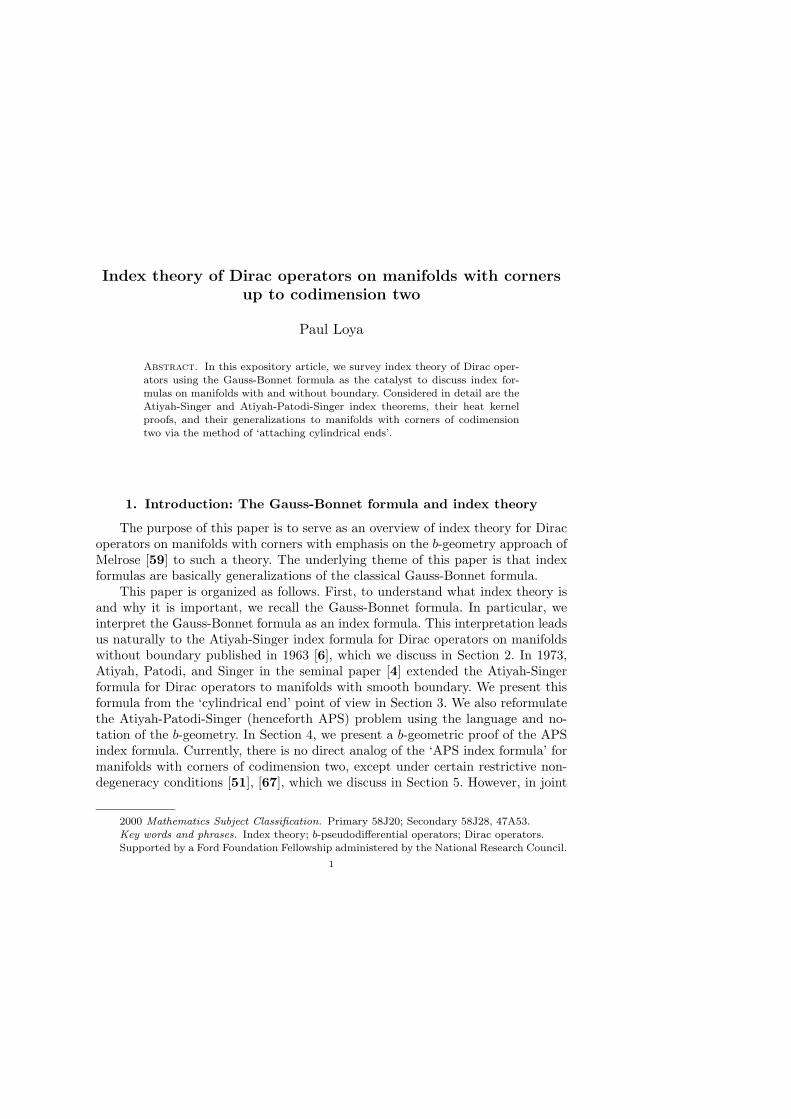
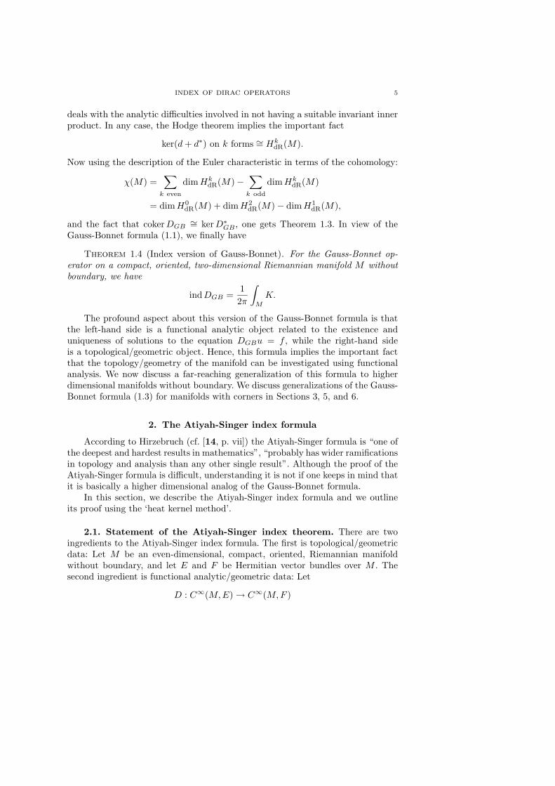
Figure 1. The manifold Pθ, where −π < θ < π, is the unitsphere with a wedge removed.
work with Melrose [53], these restrictions are removed by perturbing Dirac opera-tors using b-smoothing operators. We discuss such perturbations and the resultingindex formulas for the perturbed Dirac operators in Section 6.
Finally, I thank Gerd Grubb, Rafe Mazzeo, and Richard Melrose for helpingto make this research possible. I also thank the referees for valuable suggestions.
1.1. The classical Gauss-Bonnet formula. Let M be a compact, oriented,two-dimensional Riemannian manifold without boundary. Then the Gauss-Bonnettheorem states that
(1.1) χ(M) =1
2π
∫
M
K,
where χ(M) is the Euler characteristic of M and K is the Gaussian curvatureof M . The interesting aspect of the Gauss-Bonnet formula is that the left-handside is a topological/combinatorial object while the right-hand side is a geometricobject.1 This formula was proved by Bonnet in 1848, but is attributed also toGauss because he proved a special case of it earlier. See [68, Ch. 8] for a proof ofthe Gauss-Bonnet formula.
A natural question to ask is: Does the Gauss-Bonnet formula continue to holdif M has a smooth boundary, or more generally, if M has corners; that is, has acrooked boundary? To answer this question, we consider a concrete example. Cutout a wedge from the unit sphere producing the manifold Pθ, where −π < θ < π,as shown in Figure 1. This manifold is an example of a manifold with cornersof codimension two. Let us check if (1.1) holds verbatim for Pθ. Note that Pθ
is topologically equivalent to a disk and hence to a triangle and so has Eulercharacteristic equal to one (since the number of vertices − edges + faces = 1 for atriangle). Since the Gaussian curvature of the unit sphere is one,
∫Pθ
K = Area(Pθ).
Thus∫
PθK changes with θ: It is approximately 4π when θ is close to −π and it
decreases to 0 as θ approaches +π. Hence,
χ(Pθ) 6=1
2π
∫
Pθ
K for general θ.
Thus the Gauss-Bonnet formula (1.1) does not hold verbatim when M has corners.Intuitively, one might guess that the formula does not hold because of the presence
1The right-hand side of (1.1) turns out to be topological as well since −K/2π defines the
Chern class of M .
INDEX OF DIRAC OPERATORS 3
of the boundary and corners. In fact, one can verify directly that the followingformula does hold:
(1.2) χ(Pθ) =1
2π
∫
Pθ
K +1
2π(2θ).
The angle 2θ is called the total exterior angle of the corners. This formula is aspecial case of the general Gauss-Bonnet formula:
Theorem 1.1 (Gauss-Bonnet, 1878). Given a compact, oriented, two-dimen-sional Riemannian manifold M with corners, we have
χ(M) =1
2π
∫
M
K
+1
2π(total geodesic curvature of ∂M)
+1
2π(sum of the exterior angles at the corners).
(1.3)
Here, the geodesic curvature of ∂M measures the deviation of the smoothcomponents of ∂M from being geodesics. There is no middle term in the formula(1.2) since the smooth components of ∂Pθ are great circles, which are geodesicson the sphere. Hence, the total geodesic curvature of ∂Pθ is zero.
The Gauss-Bonnet formula in (1.3) is very beautiful as it bridges topology,geometry, and now linear algebra: The left-hand side belongs to combinatorialtopology while the first two terms on the right are geometrical and the last term islinear algebraic since it has to do with angles between vectors at the corners.Functional analysis also comes into the picture when we interpret the Gauss-Bonnet formula as an index formula. We remark that comparing the Gauss-Bonnetformula (1.1) for a manifold without boundary to the general formula (1.3), we seethat the second and third terms on the right in (1.3) can be thought of as correctionterms coming from the smooth boundary components and corners respectively.
1.2. The Gauss-Bonnet formula as an index formula. We now explainhow the Gauss-Bonnet formula can be interpreted as an index formula. We firstneed to introduce the Gauss-Bonnet operator. Let M be a compact, oriented,two-dimensional Riemannian manifold without boundary. Let
d : C∞(M,Λk) → C∞(M,Λk+1)
be the exterior derivative, where C∞(M,Λk) denotes the space of smooth k-formson M , and let
d∗ : C∞(M,Λk+1) → C∞(M,Λk)
be the adjoint of d with respect to the natural L2 inner product on k-forms givenby integration with respect to the Riemannian volume form. Let Λev = Λ0 ⊕ Λ2
be the even form bundle and Λodd = Λ1 be the odd form bundle. Then both d andd∗ map C∞(M,Λev) into C∞(M,Λodd). The operator
DGB = d + d∗ : C∞(M,Λev) → C∞(M,Λodd)
4 PAUL LOYA
is called the Gauss-Bonnet operator. By definition of the (nonnegative) Laplacian,
D∗GBDGB = ∆,
where ∆ is the Laplacian on the even forms. Thus, DGB represents in some respectsa square root of the Laplacian. For this reason DGB is called a Dirac operator afterthe physicist Paul Dirac who in the 1920’s was searching for, and found, a squareroot of the Laplacian in his efforts to quantize the electron. However, in his case,he was working with a Lorentz metric rather than a Riemannian metric.
Before presenting the index formula interpretation of the Gauss-Bonnet for-mula, we recall two results from Hodge theory. We denote the Sobolev space oforder k by Hk. So, Hk(M,Λev) consists of those even-degree forms u on M suchthat for each 0 ≤ j ≤ k, (d + d∗)ju is square integrable. Then H1(M,Λev) is thenatural domain of DGB .
Theorem 1.2. The operator DGB : H1(M,Λev) → L2(M,Λodd) is Fredholm,which means that it is ‘almost invertible’ in the sense that
(1) DGB has a finite dimensional kernel; dim ker DGB < ∞.(2) DGB has a finite dimensional cokernel;
dim coker DGB = dim(L2(M,Λodd)/Im(DGB)
)< ∞.
The first condition means that DGB is ‘almost injective’ in the sense thatit is injective up to a finite dimensional space, and the second condition meansthat DGB is ‘almost surjective’ in the sense that it is surjective up to a finitedimensional space. The index is the difference between the dimensions of the kerneland cokernel:
indDGB = dim ker DGB − dim coker DGB ∈ Z.
Theorem 1.2 follows from the fact that DGB is elliptic, and can be proved in avariety of ways, for instance, using pseudodifferential operators [34], by embeddingproperties of Sobolev spaces [74], or my favorite proof via the heat operator [9].The second result we need is:
Theorem 1.3. The index of DGB is the Euler characteristic of M ,
indDGB = χ(M).
This result can be proved using the Hodge theorem, which is described asfollows. Define the k-th deRham cohomology of M by
HkdR(M) = {α ∈ C∞(M,Λk) ; dα = 0}/{dβ ; β ∈ C∞(M,Λk−1)}.
The Hodge theorem states that given a deRham cohomology class [α] ∈ HkdR(M)
there exists a unique representative of this class β ∈ [α] such that (d+d∗)β = 0. Itis worthwhile mentioning that although the exterior derivative d is canonical, theoperator d∗ depends on the Riemannian metric chosen on the manifold. The workof Connes with Gromov and Moscovici [25] treats a branch of index theory which
INDEX OF DIRAC OPERATORS 5
deals with the analytic difficulties involved in not having a suitable invariant innerproduct. In any case, the Hodge theorem implies the important fact
ker(d + d∗) on k forms ∼= HkdR(M).
Now using the description of the Euler characteristic in terms of the cohomology:
χ(M) =∑
k even
dim HkdR(M) −
∑
k odd
dim HkdR(M)
= dim H0dR(M) + dim H2
dR(M) − dim H1dR(M),
and the fact that cokerDGB∼= ker D∗
GB , one gets Theorem 1.3. In view of theGauss-Bonnet formula (1.1), we finally have
Theorem 1.4 (Index version of Gauss-Bonnet). For the Gauss-Bonnet op-erator on a compact, oriented, two-dimensional Riemannian manifold M withoutboundary, we have
indDGB =1
2π
∫
M
K.
The profound aspect about this version of the Gauss-Bonnet formula is thatthe left-hand side is a functional analytic object related to the existence anduniqueness of solutions to the equation DGBu = f , while the right-hand sideis a topological/geometric object. Hence, this formula implies the important factthat the topology/geometry of the manifold can be investigated using functionalanalysis. We now discuss a far-reaching generalization of this formula to higherdimensional manifolds without boundary. We discuss generalizations of the Gauss-Bonnet formula (1.3) for manifolds with corners in Sections 3, 5, and 6.
2. The Atiyah-Singer index formula
According to Hirzebruch (cf. [14, p. vii]) the Atiyah-Singer formula is “one ofthe deepest and hardest results in mathematics”, “probably has wider ramificationsin topology and analysis than any other single result”. Although the proof of theAtiyah-Singer formula is difficult, understanding it is not if one keeps in mind thatit is basically a higher dimensional analog of the Gauss-Bonnet formula.
In this section, we describe the Atiyah-Singer index formula and we outlineits proof using the ‘heat kernel method’.
2.1. Statement of the Atiyah-Singer index theorem. There are twoingredients to the Atiyah-Singer index formula. The first is topological/geometricdata: Let M be an even-dimensional, compact, oriented, Riemannian manifoldwithout boundary, and let E and F be Hermitian vector bundles over M . Thesecond ingredient is functional analytic/geometric data: Let
D : C∞(M,E) → C∞(M,F )
6 PAUL LOYA
be a Dirac type operator. This means that D is an elliptic first-order differentialoperator such that “D∗D = ∆” in the sense that the principal symbol of D∗D isjust the metric σ(D∗D)(ξ) = |ξ|2 for all cotangent vectors ξ.2
The simplest example of a Dirac type operator is the Cauchy-Riemann oper-ator. Let M = R
2 with its usual Euclidean metric and let E = F = C. Then
DCR = ∂x + i∂y
is the Cauchy-Riemann operator. In this case,
D∗CRDCR =
(− ∂x + i∂y
)(∂x + i∂y
)= −
(∂2
x + ∂2y
)
is exactly the Laplacian.Another example is the higher-dimensional Gauss-Bonnet operator. Let M be
an even-dimensional, compact, oriented, Riemannian manifold without boundary,and let E and F be the even and odd degree form bundles, respectively:
E = Λev =⊕
k even
Λk and F = Λodd =⊕
k odd
Λk.
Then,DGB = d + d∗ : C∞(M,Λev) → C∞(M,Λodd)
is called the Gauss-Bonnet operator. By definition of the Laplacian on forms, wehave D∗
GBDGB = ∆, and so DGB is a Dirac operator. Since the even and odd formbundles are real bundles, they of course are technically not Hermitian, but we canalways make them so by complexifying them. Regardless, the index formula belowstill applies to the Gauss-Bonnet operator.
The celebrated Atiyah-Singer index theorem is the following.
Theorem 2.1 (Atiyah-Singer, 1963). Let D : C∞(M,E) → C∞(M,F ) bea Dirac type operator on an even-dimensional, compact, oriented, Riemannianmanifold without boundary. Then, D : H1(M,E) → L2(M,F ) is Fredholm and
(2.1) indD =
∫
M
KAS ,
where the ‘Atiyah-Singer integrand’ KAS is an explicitly defined polynomial in thecurvature forms of the manifold M and the vector bundles E and F .
The integral of the polynomial KAS is by definition the integral of the volumeform component of KAS . For those readers familiar with characteristic classes, thepolynomial KAS is the product of the A polynomial of M and the (relative) Chernpolynomials of E and F , see [9, Ch. 4]. Hence, KAS is both a topological and ageometric object. The reason why we assume that M is even-dimensional is thatfor odd-dimensional manifolds it turns out that both sides of (2.1) are zero.
Note the similarity between the index version of the Gauss-Bonnet formulagiven in Theorem 1.4 and the Atiyah-Singer formula for the index of a Dirac type
2In some occasions, we will need D to be a compatible Dirac operator, which means that
it is associated to a ‘unitary Clifford connection’. For simplicity, we leave this notion undefined,
and at the few places where we actually need this extra hypothesis, we will state so in a footnote.
INDEX OF DIRAC OPERATORS 7
operator: The Gaussian curvature in the Gauss-Bonnet formula is replaced bya polynomial in the curvature of the manifold and vector bundles. As with theGauss-Bonnet formula, the profound feature of the Atiyah-Singer formula is thatthe left-hand side of (2.1) is a functional analytic object related to the existenceand uniqueness of solutions to the equation Du = f , while the right-hand side isa topological/geometric object. In particular, the Atiyah-Singer formula has thefollowing deep consequence: It implies that the topology/geometry of a manifoldcan be investigated using functional analytic tools, cf. [72], [55], and Section 2.3.
For an application of the Atiyah-Singer index theorem, consider the Gauss-Bonnet operator defined above. As in the two-dimensional case explained beforeTheorem 1.4, for a general even-dimensional, compact, oriented, Riemannian man-ifold without boundary, Hodge theory implies that
indDGB = χ(M).
On the other hand, see [9, Ch. 4] for the details, working out the explicitly definedpolynomial KAS for E = Λev and F = Λodd gives, after a little bit of algebra,
KAS = e(M),
where e(M) is the Euler, or Pfaffian, polynomial defined by taking the n-th powerof the Riemannian curvature tensor of M and multiplying it by 1/n!× (−1/2π)n,where 2n is the dimension of M . Thus, the Atiyah-Singer index formula implies
χ(M) =
∫
M
e(M).
This generalization of the Gauss-Bonnet formula is due to Chern [23].Another important corollary of the Atiyah-Singer formula is Hirzebruch’s for-
mula for the signature of a manifold. Assume now that M is 4k dimensional. Thenthe map
H2kdR(M) × H2k
dR(M) 3 ([α ], [β ]) 7−→∫
M
α ∧ β ∈ R
is a well-defined symmetric bilinear map (here, [ · ] denotes the corresponding co-homology class). We can represent this map by a matrix by choosing any basisof the finite dimensional real vector space H2k
dR(M). The signature of this matrix,the number of positive eigenvalues minus the number of negative ones, is definedindependent of the basis chosen; the signature of the manifold, sign(M), is by def-inition the signature of the matrix with respect to any such basis. Hirzebruch [42]gives a formula for the signature:
sign(M) =
∫L(M),
where L(M) is the L-class polynomial in the curvature tensor of M . This formulais a simple corollary of the Atiyah-Singer index theorem. In this case, D is the‘signature operator’, which is equal to d + d∗ like the Gauss-Bonnet operator, butwith the vector bundles E and F being essentially certain eigenspaces of the Hodge
8 PAUL LOYA
star operator. The details can be found in [9]. For those interested readers, theL-class polynomial is given by
L(M) =
√det
( R/2πi
tanh(R/2πi)
),
where R is the Riemannian curvature tensor.Yet another classical formula that is a simple corollary of the Atiyah-Singer
index formula is the Riemann-Roch formula and its generalization to complexmanifolds, see [9], [34], [74].
2.2. Outline of the proof of the Atiyah-Singer formula. We outlinea proof of the Atiyah-Singer index theorem based on the heat kernel approachof Mckean and Singer [57] as exploited by Atiyah, Bott, and Patodi in [2]. Foraccessible versions of the proof, see [9], [34], [82]. I especially like the expositionby Roe [74].
To start off, we need the heat operators e−tD∗D and e−tDD∗
. Consider forinstance e−tD∗D. Then, for each t > 0,
e−tD∗D : C∞(M,E) → C∞(M,E),
and it is the solution operator to the heat equation for D∗D in the sense that foreach u ∈ C∞(M,E), ut = e−tD∗Du is the unique solution to the heat equation
(∂t + D∗D)ut = 0, t > 0; u0 = u.
The heat operator e−tD∗D can be defined by means of the resolvent and the func-tional calculus (cf. [34], [51]), it can be constructed asymptotically via Hadamard’smethod (cf. [9], [59]), or it can be defined using the spectrum as follows. Let {λj}be the eigenvalues of the self-adjoint operator D∗D. Then,
e−tD∗D =∑
j
e−tλj πj ,
where πj is the orthogonal projection onto the eigenspace associated to the eigen-value λj . This sum converges uniformly and absolutely and in fact, it can be usedto show that the heat operator is, for each t > 0, a smoothing operator; that is,for each t > 0 the heat operator is an integral operator with a smooth Schwartzkernel [74]. In particular, for each t > 0, the heat operator is trace class and
(2.2) e−tD∗D = πker D∗D + F (t),
where the remainder F (t) → 0 exponentially in the space of smoothing operatorsas t → ∞. A similar formula holds for e−tDD∗
.The key steps of the Mckean-Singer proof are to consider the function
h(t) = Tr(e−tD∗D) − Tr(e−tDD∗
)
INDEX OF DIRAC OPERATORS 9
and to prove the following amazing properties:
(1) limt→∞
h(t) = indD,
(2) limt→0
h(t) =
∫
M
KAS ,
(3)d
dth(t) = 0 so that h(t) is constant.
Equating the values of the constant function h(t) at t = 0 and t = ∞ proves theindex formula. Consider property (1). The formula (2.2) implies that
limt→∞
h(t) = Tr(πker D∗D) − Tr(πker DD∗)
= dim ker D∗D − dim ker DD∗.
Integration by parts shows that kerD∗D = kerD and ker DD∗ = kerD∗. Indeed,clearly ker D ⊂ ker D∗D and if (·, ·) denotes the L2 inner product, then
D∗Du = 0 ⇒ (D∗Du, u) = 0 ⇒ (Du,Du) = 0 ⇒ Du = 0.
Thus ker D∗D ⊂ ker D and so ker D∗D = kerD. Similarly, kerDD∗ = kerD∗.Thus, as coker D ∼= ker D∗, we obtain
limt→∞
h(t) = indD.
To determine the limit as t → 0 of h(t), we use the trace formulas:
Tr(e−tD∗D) =
∫
M
tr e−tD∗D(p, p) dg, Tr(e−tDD∗
) =
∫
M
tr e−tDD∗
(p, p) dg,
obtained by integrating the pointwise trace of the heat kernels restricted to thediagonal. Now the local index theorem states that3
limt→0
{tr e−tD∗D(p, p) − tr e−tDD∗
(p, p)}
= KAS(p)
uniformly in t, where the right-hand side really represents the coefficient of thevolume form component of the differential form KAS(p). This result was provedoriginally by Mckean and Singer [57] for dimension two, generalized to higherdimensions by Gilkey [32] using invariance theory, and by Patodi [70] using asuper-symmetry trick which was further developed by Alvarez-Gaume [1] in thesetting of path integrals and by Getzler [30] in a pseudodifferential setting. Thus,
(2.3) limt→0
h(t) =
∫
M
KAS .
Hence, by the fundamental theorem of calculus, we have
(2.4) indD −∫
M
KAS =
∫ ∞
0
d
dth(t) dt.
3This formula technically only applies to compatible Dirac operators, and not to arbitrary
Dirac type operators. In general, the left-hand side of (2.3) has an asymptotic expansion as t → 0
starting with negative powers of t and the right-hand side is the constant term in the expansion.
10 PAUL LOYA
We now show that ddth(t) = 0. We first claim that D∗De−tD∗D = D∗e−tDD∗
D.
To see this, let u ∈ C∞(M,E). Then, vt = D∗De−tD∗Du and wt = D∗e−tDD∗
Duagree at t = 0 and they both satisfy the equation (∂t +D∗D)ut = 0. By uniquenessof solutions to the heat equation [59, p. 271], we must have vt = wt; hence,D∗De−tD∗D = D∗e−tDD∗
D. Thus
d
dth(t) = Tr
(− D∗De−tD∗D + DD∗e−tDD∗)
= Tr(− D∗e−tDD∗
D + DD∗e−tDD∗)
= Tr([D,D∗e−tDD∗
]),
(2.5)
where [D,D∗e−tDD∗
] is the commutator of D and D∗e−tDD∗
. Using the well-knownfact that the trace vanishes on commutators of pseudodifferential operators whenat least one factor is smoothing implies that d
dth(t) = 0. Hence, according to (2.4)we have
indD =
∫
M
KAS ,
which is the Atiyah-Singer formula!
2.3. Some remarks on the Atiyah-Singer index theorem. The Atiyah-Singer index formula can be generalized to elliptic pseudodifferential operatorsusing K-theory. However, in this generality, the form KAS occurring on the right-hand side of the index formula is not explicitly defined in terms of the curvatureforms. The fact that KAS is explicitly defined in terms of the curvature forms forDirac type operators is a very special property of Dirac operators and is one of thereasons why Dirac operators are important in applications. The original proof ofthe Atiyah-Singer index theorem as sketched in [6] used cobordism theory, cf. [69].A few years later, the proof was reworked in a series of papers [7, 8]. The ‘heatkernel proof’ appeared in [2]. See [14] for a comparison of the various proofs.The Atiyah-Singer formula has been generalized to many different contexts, forexample, to families of Dirac operators by Bismut [11], see [74], [9], and especially[34, Ch. 5] for other generalizations.
The Atiyah-Singer index theorem has far-reaching applications (see [45, Ch. 4])that include group actions on manifolds, immersions into Euclidean space, inte-grality and divisibility of certain characteristic numbers, existence of metrics withpositive scalar curvature [37], twisted signature and Riemann-Roch-Hirzebruchformulas, and formal dimensions of certain moduli spaces [27, 36].
3. The Atiyah-Patodi-Singer index formula
Now we ask a similar question concerning the Atiyah-Singer index formulaas we did for the Gauss-Bonnet formula in the introduction: Does the Atiyah-Singer formula, indD =
∫M
KAS , continue to hold verbatim if M has a smoothboundary? From our experience with the Gauss-Bonnet formula, we expect thatthe answer is “no”; there should be a correction term added to the right-hand side
INDEX OF DIRAC OPERATORS 11
� �� �� � � � ��
� ��� � �
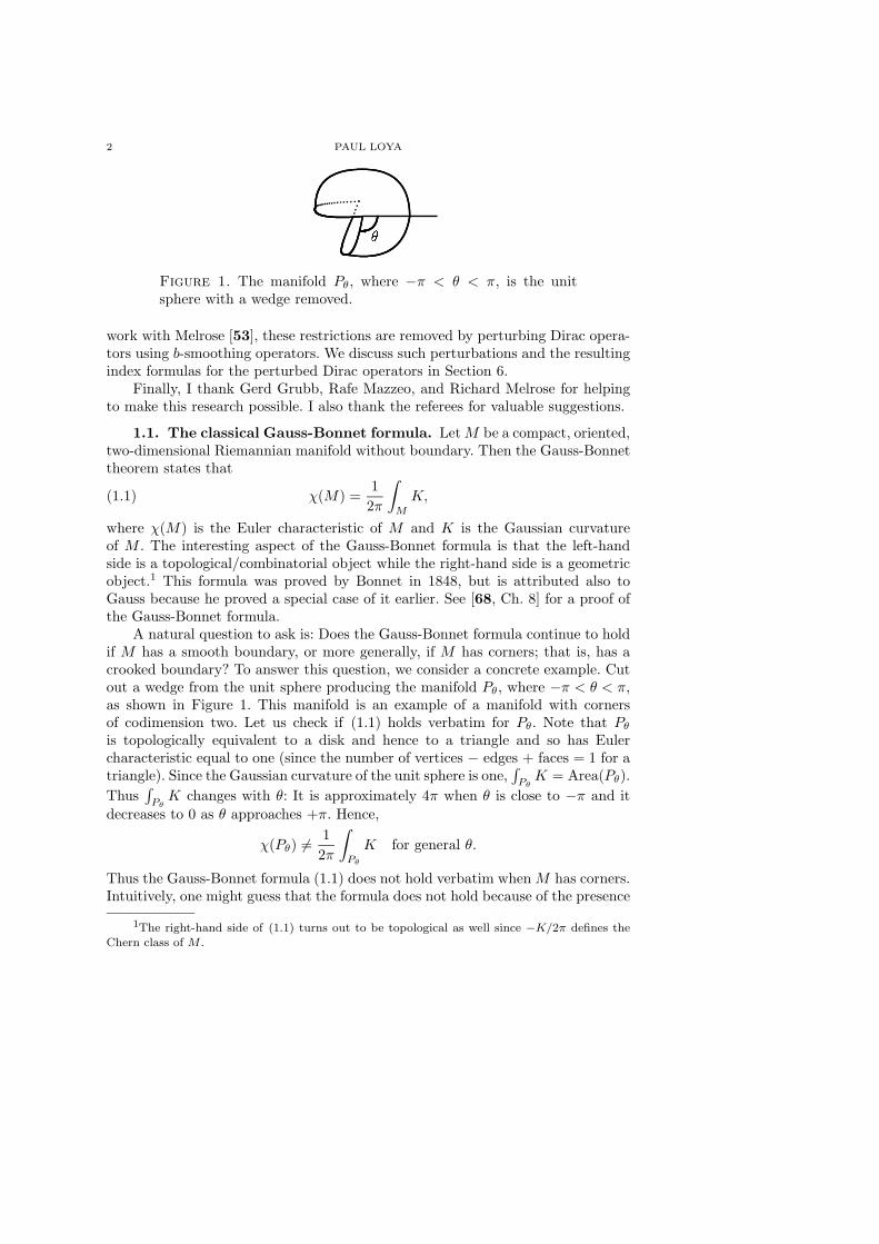
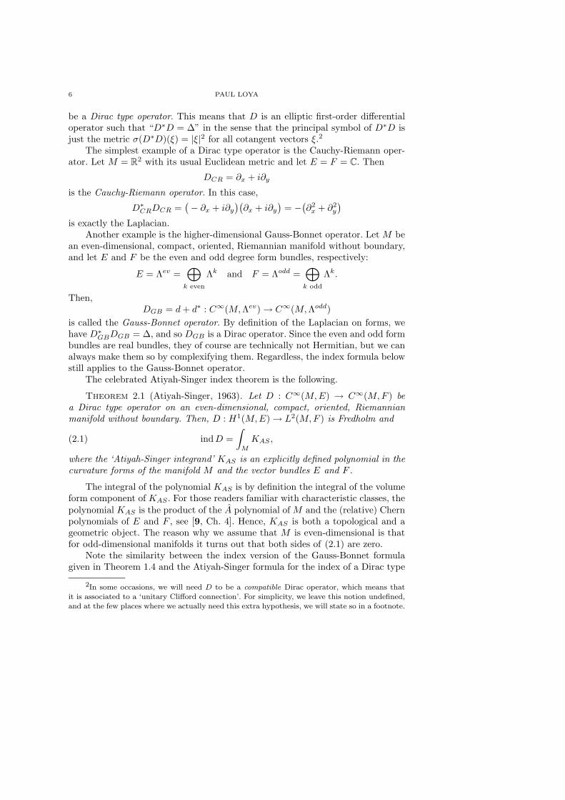
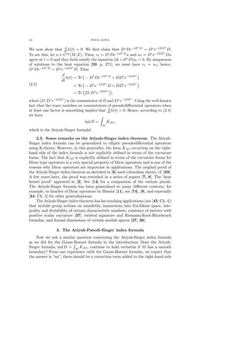
Figure 2. The manifold M with a collar neighborhood near itsboundary over which all geometric structures are of product type.
due to the presence of the boundary. This is in fact the case. It turns out that thecorrection term is a spectral invariant of the boundary.
In this section, we describe the Atiyah-Patodi-Singer (or APS) index formula[5], which extends the Atiyah-Singer formula to manifolds with boundary. Formanifolds with boundary, there are various ways to develop an index theory, forinstance, introducing boundary conditions or ‘attaching a cylindrical end’ to theboundary. We focus on the latter method. For the BVP point of view, see [15]. Fi-nally, we reformulate the index problem in terms of Melrose’s b-geometric objects.
3.1. Attaching a cylindrical end. The ingredients of the APS index for-mula include topological/geometric data: Let M be an even-dimensional, compact,oriented, Riemannian manifold with boundary and let E and F be Hermitian vec-tor bundles over M . For simplicity, we assume that M has a collar neighborhoodM ∼= [0, 1)s × Y where the metric is a product g = ds2 + h with h a metric onY = ∂M , and where E and F are isomorphic to their restrictions E0 and F0
respectively to Y over this collar. See Figure 2.We are also given functional analytic/geometric data: Let
D : C∞(M,E) → C∞(M,F )
be a Dirac type operator, a first-order elliptic differential operator such that theprincipal symbol of D∗D is the metric σ(D∗D)(ξ) = |ξ|2 for all cotangent vectorsξ. We assume that D is of product type on the collar of the following sort:
D = Γ(∂s + DY ),
whereDY : C∞(Y,E0) → C∞(Y,E0)
is a self-adjoint Dirac type operator on the odd-dimensional manifold Y , and whereΓ is a unitary isomorphism from E0 onto F0. With these hypotheses, one mightthink that D : H1(M,E) → L2(M,F ) is Fredholm. This however is not the case.
Theorem 3.1. The Dirac type operator
D : H1(M,E) → L2(M,F )
is never Fredholm. In fact, its kernel is infinite dimensional!
12 PAUL LOYA
�� �
�� �� ��� � ��� �
��
!"#$%&'$!(# )%& !*+,(!- )%&
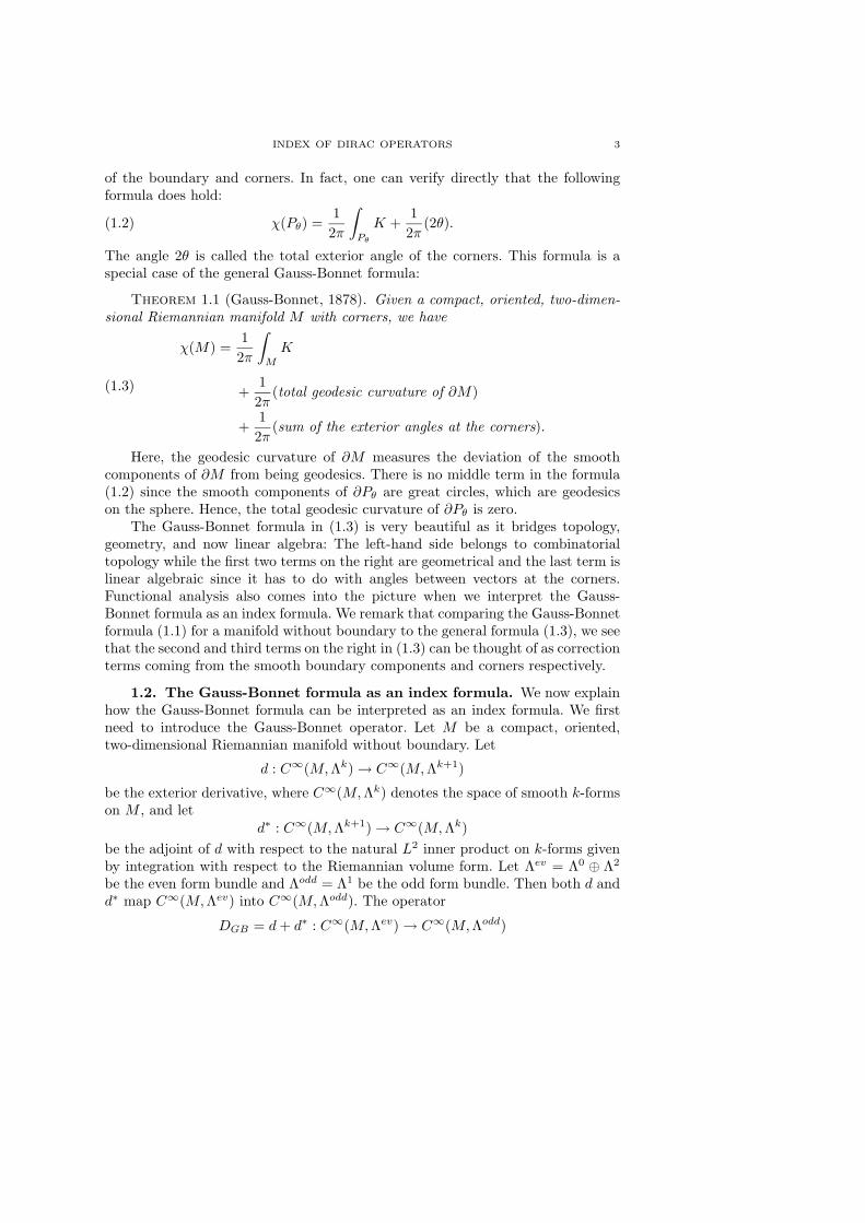
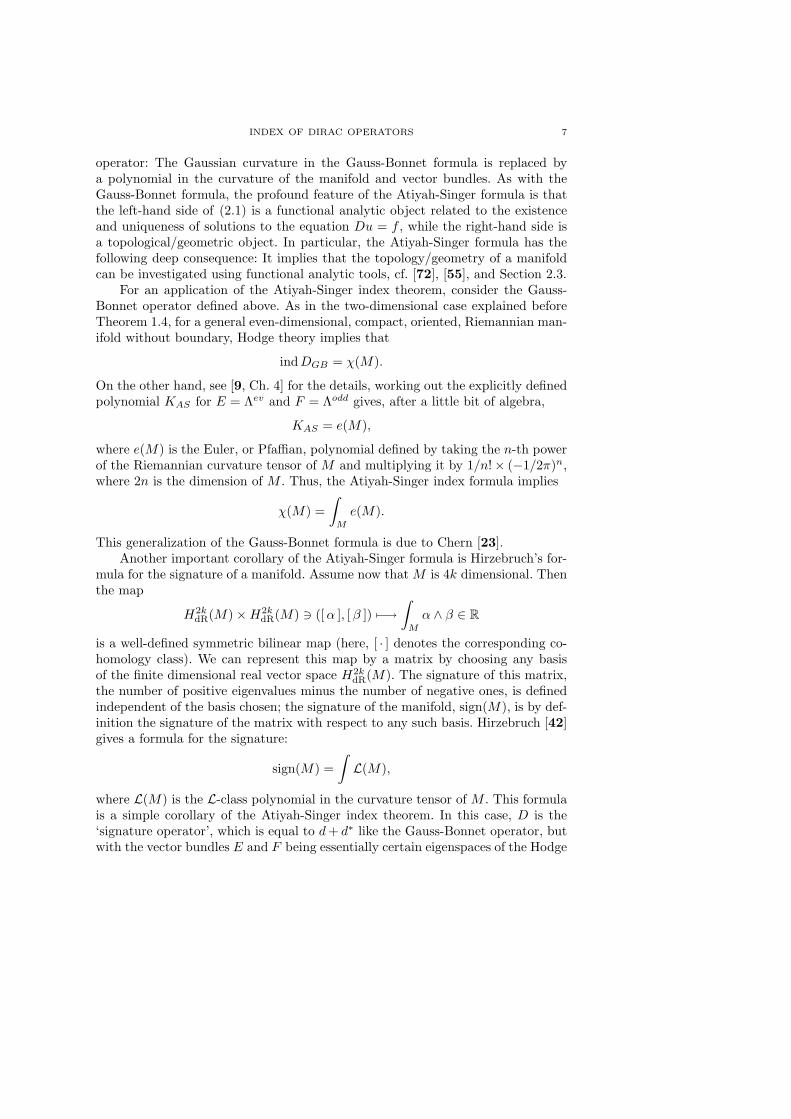
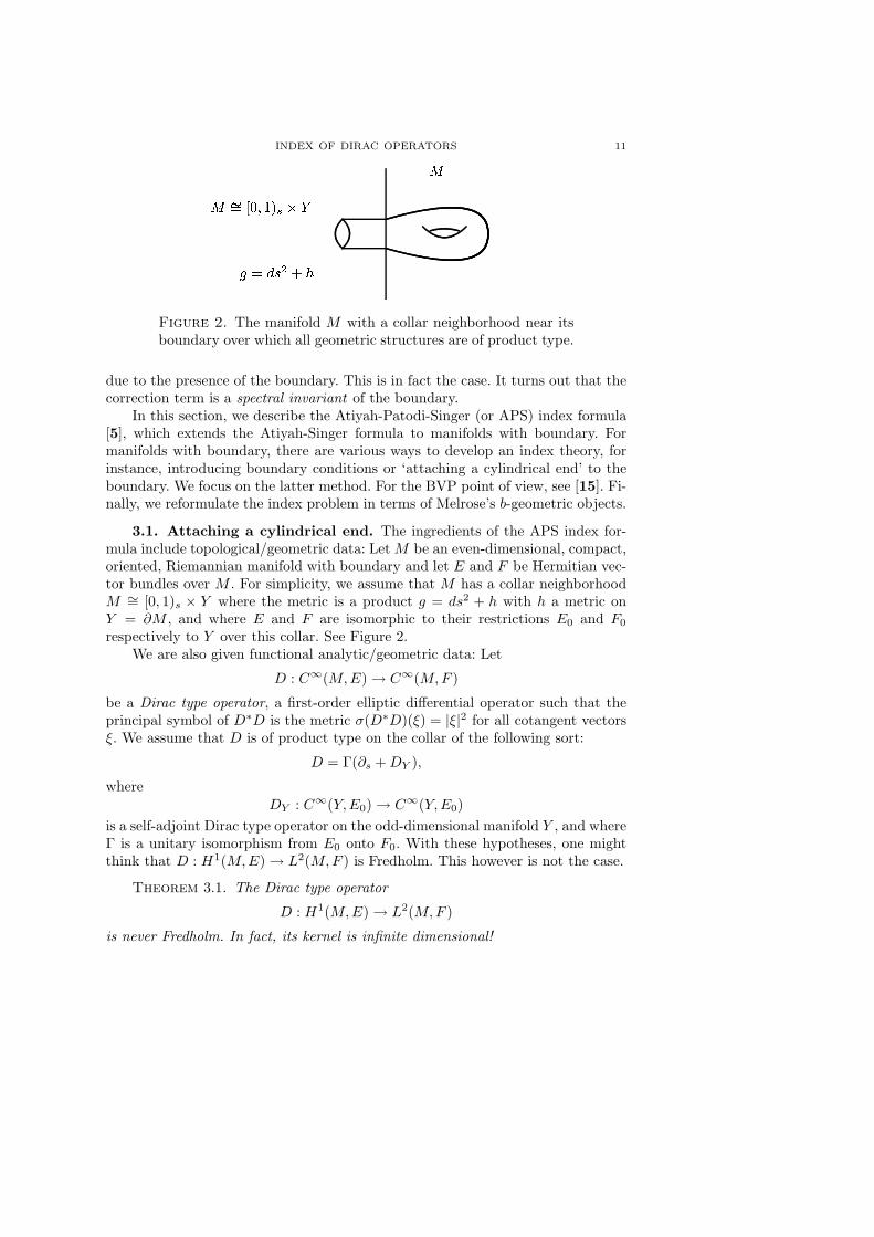
Figure 3. Attaching an infinite cylinder to M produces the man-
ifold with cylindrical end M .
A proof of Theorem 3.1 can be found in [15]. To see why this theorem holds,consider the following simple example. Let M0 = [0, 1] × S
1 with metric g =ds2 + dθ2, let E = F = C, and let
D0 = ∂s + i∂θ.
Certainly, the manifold and operator are of product type. Moreover, kerD0 consistsof all functions f(s, θ) that are holomorphic in z = s+iθ for 0 ≤ s ≤ 1 and periodicin θ with period 2π. Of course, there are infinitely many such functions, for exampleekz where k ∈ Z. Thus, dim kerD0 = ∞.
Since D is not Fredholm, it might look like our hopes for an index formulaare crushed. By the way, it turns out that in general, D : H1(M,E) → L2(M,F )is surjective [15]. Thus, the problem with D is its kernel on H1(M,E). There arevarious ways that have been developed to ‘tame’ the infinite dimensional kernel.One successful method is the theory of boundary value problems pioneered byCalderon [19] and Seeley [77] as explained in [15]. However, we will focus on themethod of attaching a cylindrical end, which is described as follows.
Consider D0 = ∂s + i∂θ on the enlarged manifold M0 = (−∞,∞)s ×S1 rather
than on M0 = [0, 1]s×S1. Here, M0 has the naturally extended metric g = ds2+dθ2.
We claim that on M0, we have ker D0 = 0 on H1(M0). Indeed, ker D0 consists of
all functions f(s, θ) ∈ H1(M0) that are holomorphic in z = s + iθ for s ∈ R andperiodic in θ with period 2π. By Sobolev embedding, f is bounded in s and henceis a bounded holomorphic function on C, so is constant by Liouville’s theorem.
Since f ∈ H1(M0), the constant must be zero.With this example as motivation, in the general case we enlarge the compact
manifold with boundary M to a noncompact manifold M as follows: Let M be themanifold formed by taking the infinite cylinder (−∞, 0]s × Y and gluing it ontothe end of the collar [0, 1)s × Y of M as shown in Figure 3:
M = (−∞, 0]s × Y t∂M M.
Since all the geometric structures and the Dirac operator were of product type on
the collar of M , they all have natural extensions to the manifold M . We denote
these extended structures on M using the same notations for the original objects on
INDEX OF DIRAC OPERATORS 13
M ; however, since the extended Dirac operator on M has a completely differentdomain than the Dirac operator on M , we denote the extension of the Dirac
operator by D. Note that the natural domain of D is H1(M,E), which consists
of those sections u on M such that Du is square integrable with respect to the
measure dg on M . Now we ask: Does this idea work? Is the operator D Fredholmon its natural domain? The answer is: sometimes. It turns out that the boundary
operator DY , which can be considered the model operator for D ‘at infinity’ onthe cylindrical end, determines the Fredholm condition.
Theorem 3.2. The Dirac type operator
D : H1(M,E) → L2(M, F )
is Fredholm if and only if the boundary operator DY : H1(Y,E0) → L2(Y,E0) isinvertible; that is, if it has zero kernel.
It turns out that the kernel of D is always finite dimensional, so the enlarge-
ment of M to M did tame the infinite dimensional kernel of D as expected, but the
cokernel of D is infinite dimensional unless DY is invertible. For a proof of Theo-rem 3.2, see [59, Th. 5.60]. There is a general principle underlying the Fredholmproperties of Dirac operators on noncompact manifolds:
General Principle: A Dirac operator on a noncompact
manifold is Fredholm if and only if it is invertible ‘at infinity’.(3.1)
Recall that a Fredholm operator is an operator that is ‘almost invertible’. Roughlyspeaking, a Dirac operator is always ‘almost invertible’ on the ‘compact end’ of anoncompact manifold simply because a Dirac operator is elliptic so we can alwaysconstruct a parametrix for it on the compact end; however, to construct a globalparametrix for the Dirac operator, we need to invert the Dirac operator ‘at infinity’.
We now show that Dirac operators can always be made Fredholm on weightedSobolev spaces. To see this, extend the coordinate function s on the cylindrical
end of M into the compact end of M to be a positive function there. Let α ∈ R.Then observe that on the cylindrical end we have
e−αsD eαs = Γ(∂s + DY + α),
and DY + α is invertible for |α| > 0 less than the smallest absolute value of anonzero eigenvalue of DY . Hence, the ‘General Principle’ implies that
e−αsDeαs : H1(M,E) → L2(M, F )
is Fredholm for all |α| > 0 sufficiently small, which is equivalent to
D : eαsH1(M,E) → eαsL2(M, F )
is Fredholm on weighted Sobolev spaces. Thus we have the following:
14 PAUL LOYA
Theorem 3.3. There exists a δ > 0 such that for all 0 < |α| < δ, the Diractype operator
D : eαsH1(M,E) → eαsL2(M, F )
is Fredholm.
For the proof of this theorem, see [59, Th. 5.60]. We next state the APS
formula for the index of the operator D on weighted Sobolev spaces.
3.2. Statement of the Atiyah-Patodi-Singer index theorem. Before
stating the APS index theorem for the operator D, we first need to define theeta invariant. Since DY is a self-adjoint elliptic operator on the closed compactmanifold Y , it has discrete spectrum {λj} ⊂ R. The eta function, η(z), is theholomorphic function
η(z) =∑
λj 6=0
sign λj
|λj |z.
One of the main results of [5] was that η(z) defines a meromorphic function on C
that is regular at z = 0. The eta invariant of DY is the value of the eta functionat zero, η(DY ) = η(0), which represents a formal signature of the operator DY :
“ η(DY ) =∑
λj 6=0
sign λj = #{λj > 0} − #{λj < 0} ”.
Thus, η(DY ) is a measurement of the spectral asymmetry of DY . Another way toexpress the eta function is through the heat operator:
(3.2) η(z) =1
Γ( z+12 )
∫ ∞
0
tz−1
2 Tr(DY e−tD2Y ) dt,
where Γ(z) is the Gamma function. This formula follows from the fact that
Tr(DY e−tD2Y ) =
∑
λj 6=0
λj e−tλ2j
and that
1
Γ( z+12 )
∫ ∞
0
tz−1
2 λj e−tλ2j dt =
λj
|λj |z+1
1
Γ( z+12 )
∫ ∞
0
tz−1
2 e−t dt =sign λj
|λj |z,
where we made the change of variables t 7→ t/|λj |2. Moreover, the local indextheorem for odd-dimensional manifolds proved by Bismut and Freed [10] states
that Tr(DY e−tD2Y ) is a smooth function of t1/2 vanishing at t = 0, and so the
INDEX OF DIRAC OPERATORS 15
formula (3.2) can be used to prove that4
(3.3) η(DY ) =1√π
∫ ∞
0
t−1/2 Tr(DY e−tD2Y ) dt.
We are now ready to state the Atiyah-Patodi-Singer index theorem.
Theorem 3.4 (Atiyah-Patodi-Singer, 1973). Let D be a Dirac type operatoron an even-dimensional, compact, oriented, Riemannian manifold with boundarywith product type structures specified. Then there exists a δ > 0 such that for all0 < |α| < δ, the Dirac type operator
D : eαsH1(M,E) → eαsL2(M, F )
is Fredholm and if its index is denoted by indα D, then
indα D =
∫
M
KAS − 1
2
{η(DY ) + sign α · dim kerDY
},
where KAS is the Atiyah-Singer integrand and η(DY ) is the eta invariant.
The APS theorem in [5] technically only applies to the case of α > 0; aspresented above, the theorem is due to Melrose [59]. We prove this theorem usingMelrose’s b-geometry approach in Section 4. An important corollary is the notablegeneralization of Hirzebruch’s signature formula to manifolds with boundary: If D
is the signature operator, then using the fact that indα D + ind−α D = 2 sign(M)for α > 0 sufficiently small (see [59, Sec. 9.3]) gives
2 sign(M) =
∫
M
L(M) − 1
2
{η(DY ) + dim kerDY
}
+
∫
M
L(M) − 1
2
{η(DY ) − dim ker DY
},
or
sign(M) =
∫
M
L(M) − 1
2η(DY ).
Hirzebruch’s conjecture for the signature-defect, the difference between the signa-ture of M and the integral of the L-class polynomial, was the original motivationof Atiyah, Patodi, and Singer in the discovery of the eta invariant [4, 5].
4Actually, the local index theorem for odd-dimensional manifolds is not true for arbitraryDY but only for those associated to a ‘unitary Clifford connection’, cf. the discussion in footnote
(3) concerning the local index theorem for even-dimensional manifolds. In general, Tr(DY e−tD2Y )
only has an asymptotic expansion as t → 0 starting from negative powers of t. In this case, thelower limit 0 in the integral (3.3) must be replaced by ε > 0 and the resulting integral has
an asymptotic expansion as ε → 0. The right-hand side of the above equation represents the
constant term in the expansion.
16 PAUL LOYA
.// 0
1212 34 567 8 9:; < 0 = 34 >9 8 ?:@ < 0=
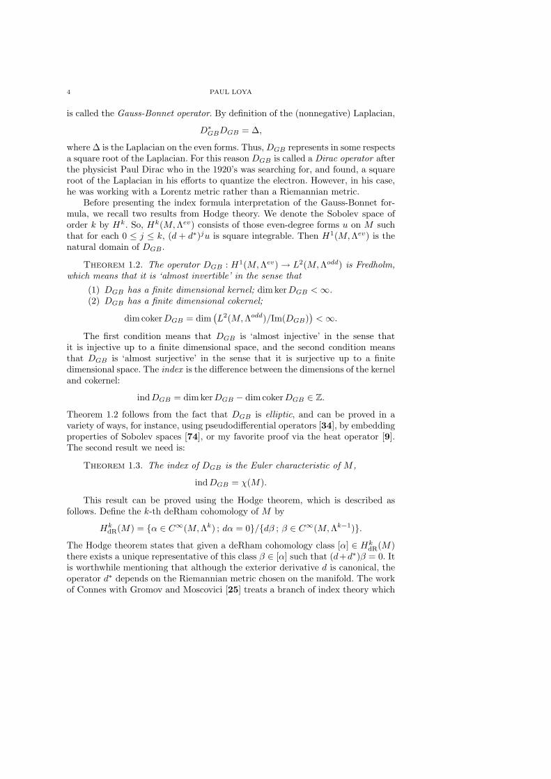
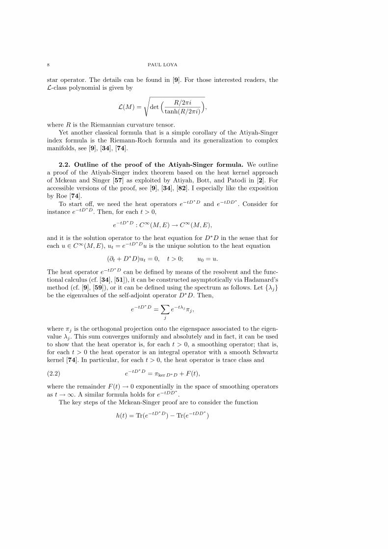
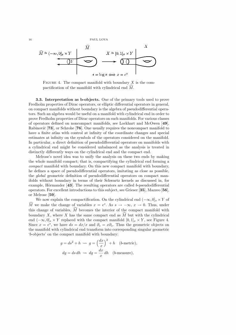
A 4 BCD E FG E 4 H;Figure 4. The compact manifold with boundary X is the com-
pactification of the manifold with cylindrical end M .
3.3. Interpretation as b-objects. One of the primary tools used to proveFredholm properties of Dirac operators, or elliptic differential operators in general,on compact manifolds without boundary is the algebra of pseudodifferential opera-tors. Such an algebra would be useful on a manifold with cylindrical end in order toprove Fredholm properties of Dirac operators on such manifolds. For various classesof operators defined on noncompact manifolds, see Lockhart and McOwen [49],Rabinovic [73], or Schrohe [76]. One usually requires the noncompact manifold tohave a finite atlas with control at infinity of the coordinate changes and specialestimates at infinity on the symbols of the operators considered on the manifold.In particular, a direct definition of pseudodifferential operators on manifolds witha cylindrical end might be considered unbalanced as the analysis is treated indistinctly differently ways on the cylindrical end and the compact end.
Melrose’s novel idea was to unify the analysis on these two ends by makingthe whole manifold compact; that is, compactifying the cylindrical end forming acompact manifold with boundary. On this new compact manifold with boundary,he defines a space of pseudodifferential operators, imitating as close as possible,the global geometric definition of pseudodifferential operators on compact man-ifolds without boundary in terms of their Schwartz kernels as discussed in, forexample, Hormander [43]. The resulting operators are called b-pseudodifferentialoperators. For excellent introductions to this subject, see Grieser [35], Mazzeo [56],or Melrose [59].
We now explain the compactification. On the cylindrical end (−∞, 0]s × Y of
M we make the change of variables x = es. As s → −∞, x → 0. Thus, under
this change of variables, M becomes the interior of the compact manifold with
boundary X, where X has the same compact end as M but with the cylindricalend (−∞, 0]s × Y replaced with the compact manifold [0, 1]x × Y , see Figure 4.Since x = es, we have ds = dx/x and ∂s = x∂x. Thus the geometric objects onthe manifold with cylindrical end transform into corresponding singular geometric‘b-objects’ on the compact manifold with boundary:
g = ds2 + h g =(dx
x
)2
+ h (b-metric),
dg = ds dh dg =dx
xdh (b-measure),
INDEX OF DIRAC OPERATORS 17
and consequently,
Hk(M) Hkb (X) (b-Sobolev space),
D = Γ(∂s + DY ) D = Γ(x∂x + DY ) (b-differential operator).
Although the manifold X is topologically compact, its interior is geometrically amanifold with cylindrical end since X inherited all its geometric structures from
M . In particular, the boundary of X is geometrically at infinity. The fact thatX is compact is key to the definition of b-pseudodifferential operators since theseoperators are defined using only the usual classes of smooth functions and dis-tributions on compact manifolds with boundary. Of course, there is a trade off:The distributions defining the Schwartz kernels of b-pseudodifferential operatorsare required to have a special structure, which takes some time getting used to[59, Ch. 4].
We repeat the statement of the APS index theorem in the current context.
Theorem 3.5. With the same hypotheses as in Theorem 3.4, but now in theb-geometry context, there exists a δ > 0 such that for all 0 < |α| < δ, the Diractype operator
D : xαH1b (X,E) → xαL2
b(X,F )
is Fredholm and if its index is denoted by indα D, then
indα D =
∫
M
KAS − 1
2
{η(DY ) + sign α · dim kerDY
},
where KAS is the Atiyah-Singer integrand and η(DY ) is the eta invariant
η(DY ) =1√π
∫ ∞
0
t−1/2Tr(DY e−tD2Y ) dt.
In Section 4, we prove this theorem.
3.4. Some remarks on the Atiyah-Patodi-Singer index theorem. Theoriginal Atiyah-Patodi-Singer index theorem was proved in the context of (pseudo-differential) boundary value problems. A nice introduction to these methods can befound in the book by Booß-Bavnbek and Wojciechowski [15]. The ‘direct approach’to the APS boundary value problem based on asymptotic expansions of the heatoperator was initiated by Grubb and Seeley [39], see also Grubb’s book [38]. Theapproach of ‘attaching cylinders’ was mentioned in [5], but was not developed.Besides attaching a cylinder to the boundary, another way to develop an indextheory on manifolds with boundary is by attaching a cone, see Cheeger [22]; forother generalizations, see Atiyah, Donnelly, and Singer [3], Muller [64], Stern [81],Bruning [16], Fedosov and Schulze [29], Schulze, Sternin, and Shatalov [79], andCarron [21]. Melrose introduced the b-geometry in the seminal paper [58], andthese ideas were developed by Melrose and Mendoza in [60]. The APS index for-mula was generalized to Fredholm b-pseudodifferential operators by Piazza [71].
The eta invariant itself has become a topic of much interest. In particular, theextension of the eta function and its regularity properties for pseudodifferential
18 PAUL LOYA
operators has been examined by Gilkey [33] and Wodzicki [85] among others. Fora survey of various topics on the eta invariant, including its decomposition undergluing of manifolds, see Mazzeo and Piazza [55].
The index theorem for families of Dirac operators was extended to the casewhen the fibers are manifolds with boundary by Bismut and Cheeger [12, 13] un-der the assumption that the Dirac operators on the fibers of the boundary fibrationare invertible. Later, this result was generalized by Melrose and Piazza [62, 63]with no assumptions on the boundary Dirac operators. For further extensions ofthe index formula, see Getzler [31], Wu [86], Melrose and Nistor [61], and Leicht-nam, Lott, and Piazza [46].
Other expository articles incorporating recent developments on the APS in-dex theorem include Muller [66], Piazza [72], and Seeley [78]. Because of spaceconstraints, we have only touched the surface on some of the many extensions andgeneralizations of the Atiyah-Patodi-Singer problem, a list of references can befound in the book by Gilkey [34, Ch. 5].
4. Melrose’s b-geometry proof of the Atiyah-Patodi-Singer theorem
Let D be a Dirac type operator on an even-dimensional, compact, oriented,Riemannian manifold with boundary M with product type structures near theboundary as described in Section 3.1. For simplicity, we assume that the boundary
Dirac operator DY is invertible. Now form the manifold with cylindrical end Mand then compactify it under the change of variables x = es, where s is the variable
on the cylinder, to form the manifold X as described in Section 3.3. Then D definesan operator on X such that
D : H1b (X,E) → L2
b(X,F )
is Fredholm. We now give the b-geometry proof of the APS index formula inTheorem 3.5 modeling, as close as possible, the proof the Atiyah-Singer formulagiven in Section 2.2. We shall see that there are certain variations to the proofthat need to be fleshed out in order to make the proof work.
4.1. The proof of APS with details left out. As with the Atiyah-Singerproof given in Section 2.2, we would like to define the Mckean-Singer function
“ Tr(e−tD∗D) − Tr(e−tDD∗
)”.
Here, we meet our first variation to the Atiyah-Singer proof – the reason for thequotation marks is that the heat operators are not trace class, and so the traces arenot even defined! Basically, the heat operators are not trace class because X hasinfinite volume (is geometrically not compact) which implies that the heat kernelsrestricted to the diagonal are not integrable. Thus, we cannot prove the APSformula by imitating the proof of the Atiyah-Singer formula verbatim. However,in Section 4.3, we define a natural extension of the trace called the b-trace, denoted
INDEX OF DIRAC OPERATORS 19
by bTr, such that the heat operators are b-trace class. We can now define a modifiedMckean-Singer function
h(t) = bTr(e−tD∗D) − bTr(e−tDD∗
),
and continue as in Section 2.2. As in the manifold without boundary case, thefollowing limits hold:
limt→∞
h(t) = ind D,
and5
limt→0
h(t) =
∫
M
KAS .
In fact, using b-pseudodifferential operators, the proofs of these two results are notmuch different from the corresponding proofs in the manifold without boundarycase, see Chapters 7 and 8 of [59] for the proofs. Continuing as in Section 2.2, wefind that
ind D =
∫
M
KAS +
∫ ∞
0
d
dth(t) dt,
where repeating the same algebraic calculation as before, we have
d
dth(t) = bTr
([D, D∗e−tDD∗
]).
Here, we meet our second variation – in the proof of the Atiyah-Singer index for-mula, this expression is zero, in this present case it is not. Figuratively speaking,the b-trace is a trace on the interior of X and only fails to be a trace on the bound-
ary of X. Thus intuitively, bTr([D, D∗e−tDD∗
])
should be a boundary integral ofsome sort. This is in fact the case; in Section 4.4 we compute that
bTr([D, D∗e−tDD∗
])
= − 1√4πt
Tr(DY e−tD2Y ) =
1
2√
πt−1/2 Tr(DY e−tD2
Y ).
Hence,
ind D =
∫
X
KAS − 1
2η(DY ),
where
η(DY ) =1√π
∫ ∞
0
t−1/2 Tr(DY e−tD2Y ) dt,
and the Atiyah-Patodi-Singer index formula is proved!
5The same discussion as in footnote (3) concerning the local index theorem on manifoldswithout boundary applies in this situation too. The integral of KAS is over M because the
product type assumption implies that the volume form component of KAS is supported on the
manifold M regarded as a subset of X.
20 PAUL LOYA
4.2. Some facts about the heat kernels. To implement the proof in Sec-tion 2.2, we need the heat operators
e−tD∗D : L2b(X,E) → H2
b (X,E) and e−tDD∗
: L2b(X,F ) → H2
b (X,F ).
It turns out that these heat operators are b-smoothing operators; that is, they areb-pseudodifferential operators of order −∞ [59, Ch. 7], which implies a couple ofuseful results. These results can be proved using other methods, but the theory ofb-pseudodifferential operators gives these results more or less ‘for free’. First, theSchwartz kernels of these heat operators are smooth on the interior of X2 vanishingto infinite order at ∂X2 except at ∂X × ∂X. The second result is that these heatoperators have a simple structure on the collar of X described as follows. For
concreteness, we focus on e−tDD∗
. On the collar [0, 1]x × Y of X we have
D = Γ(x∂x + DY ),
where Γ is a unitary isomorphism of E0 onto F0. Thus, on the collar,
DD∗ = Γ(x∂x + DY )(−x∂x + DY )Γ∗ = Γ((xDx)2 + D2Y )Γ∗,
where Dx = i−1∂x. This suggests that near ∂X we have
e−tDD∗
= Γe−t(xDx)2e−tD2Y Γ∗ + O(x),
where e−t(xDx)2 is the heat operator for xDx on [0,∞)x, and where O(x) is anoperator smooth in x and vanishing at x = 0. In fact, even a stronger result is true.Under the change of variables s = log x, which takes the interior of [0,∞)x onto
(−∞,∞)s, we have xDx = Ds. Since the Schwartz kernel of e−tD2s on (−∞,∞)s
is given by the well-known formula
K1(s, s′, t) =
1√4πt
e−(s−s′)2/4t,
the Schwartz kernel of e−t(xDx)2 is obtained by setting s = log x:
K1(x, x′, t) =1√4πt
e−(log x−log x′)2/4t.
The second result is that the Schwartz kernel of e−tDD∗
near ∂X ×∂X is given by
(4.1) e−tDD∗
(x, y, x′, y′) = Γ(y)K1(x, x′, t) e−tD2Y (y, y′) Γ(y′)∗ + O(x),
where O(x) is a smooth function of the variables x, log x − log x′, y, and y′ thatvanishes at x = 0.
4.3. Filling in the details for the b-trace. The simple fact that dx/xis not integrable over [0, 1]x implies that the heat operators are not trace class.
Indeed, consider the heat operator e−tDD∗
. By (4.1), on the collar [0, 1]x × Y wehave
(4.2) tr e−tDD∗
(x, y, x, y) =1√4πt
tr e−tD2Y (y, y) + O(x),
INDEX OF DIRAC OPERATORS 21
where we used that ΓΓ∗ = Id since Γ is a unitary isomorphism, and where O(x)is smooth in x and vanishes at x = 0. Since dg = (dx/x) dh on this collar and
∫
[0,1]×Y
tr e−tD2Y (y, y)
dx
xdh =
(∫ 1
0
dx
x
)·∫
Y
tr e−tD2Y (y, y) dh,
the following trace formula does not make sense:
Tr(e−tDD∗
) =
∫
X
tr e−tDD∗
(p, p) dg.
Similarly, the corresponding integral for e−tD∗D does not exist. Although the traceformula above does not make sense, we can ‘force’ it to make sense by the con-sidering another notion of trace and integral as we now describe. Note that forRe z > 0, xz is integrable with respect to dx/x over [0, 1]x. Extend the coordinatefunction x on the collar of X to be a smooth function on X which is positive off
the collar. Then it follows that xze−tDD∗
is trace class for Re z > 0 with tracegiven by
Tr(xze−tDD∗
) =
∫
X
xz tr e−tDD∗
(p, p) dg, Re z > 0.
This argument is the basis for defining a new functional called the b-trace, whichwe introduce after the following lemma.
Lemma 4.1. Let f ∈ C∞(X). Then for all complex numbers z with Re z > 0,the integral
F (z) =
∫
X
xzf dg
exists, and it extends from Re z > 0 to define a meromorphic function on all of C.The b-integral of f is by definition the regular value of F (z) at z = 0:
(4.3) b
∫
X
f dg = Regz=0 F (z).
Finally, the residue of F (z) at z = 0 given by
Resz=0 F (z) =
∫
Y
f(0, y) dh.
To understand why this lemma is true, note that xz = ez log x is an entirefunction of z for x > 0. Thus, we may assume that f is supported on the collar[0, 1]x×Y of X. Then F (z) is well defined for Re z > 0 since xzf(x, y) is integrablewith respect to the measure (dx/x) dh as long as Re z > 0. Now expand f(x, y) inTaylor series at x = 0: f(x, y) ∼ ∑∞
k=0 xkfk(y). Since∫
[0,1]×Y
xz+kfk(y)dx
xdh =
1
z + k
∫
Y
fk(y) dh
22 PAUL LOYA
it follows that F (z) extends from Re z > 0 to be a meromorphic function on C
with only simple poles at z = {0,−1,−2, . . .} with residue at z = 0 given by∫
Y
f0(y) dh =
∫
Y
f(0, y) dh.
To see why the notion of the b-integral is natural, note that if f(0, y) = 0,then F (z) is regular at z = 0, and
b
∫
X
f dg = Regz=0 F (z) = F (0) =
∫
X
f dg,
which is the usual integral of f .
The b-trace of the heat operator e−tDD∗
is by definition
bTr(e−tDD∗
) = b
∫
X
tr e−tDD∗
(p, p) dg,
where the b-integral of the function tr e−tDD∗
(p, p) is defined by (4.3):
b
∫
X
tr e−tDD∗
(p, p) dg = Regz=0 Tr(xze−tDD∗
).
The b-trace of e−tD∗D is defined similarly.
4.4. Filling in the details for the eta invariant. In this section, we showthat
bTr([D, D∗e−tDD∗
])
= − 1√4πt
Tr(DY e−tD2Y ).
The proof is just a computation using the definition of the b-trace,
bTr([D, D∗e−tDD∗
])
= Regz=0 Tr xz[D, D∗e−tDD∗
],
where Tr xz[D, D∗e−tDD∗
] is meromorphically extended from Re z > 0. Observethat
xz[D, D∗e−tDD∗
] = [xz, D]D∗e−tDD∗
+ [D, xzD∗e−tDD∗
].
Since the trace vanishes on commutators, we have Tr[D, xzD∗e−tDD∗
] = 0 forRe z > 0, and thus its meromorphic extension to all of C is also zero. Hence,
bTr([D, D∗e−tDD∗
])
= Regz=0 Tr[xz, D]D∗e−tDD∗
= Regz=0 Tr xza(z),
where
a(z) = x−z[xz, D]D∗e−tDD∗
= DD∗e−tDD∗ − x−zDxzD∗e−tDD∗
.
Note that a(0) = 0. We claim that a(z) is an entire function of z. Indeed, since xz
is an entire function of z for x > 0, we may consider a(z) on the collar [0, 1]x × Y
over which D = Γ(x∂x + DY ). In this case, x−zDxz = Γ(x∂x + DY + z) which isentire, so a(z) is entire. Since a(z) is entire and vanishes at z = 0, we can write
a(z) = zA + O(z2),
INDEX OF DIRAC OPERATORS 23
where A is independent of z. It follows that
bTr([D, D∗e−tDD∗
])
= Regz=0 Tr xza(z) = Resz=0 Tr xzA,
and so by Lemma 4.1,
(4.4) bTr([D, D∗e−tDD∗
])
=
∫
Y
tr A(x, y, x, y)|x=0 dh.
To calculate this integral, we work over the collar [0, 1]x × Y . Here,
x−zDxz = Γ(x∂x + DY + z) = D + z Γ,
and thus
a(z) = DD∗e−tDD∗ − x−zDxzD∗e−tDD∗
= −zΓD∗e−tDD∗
,
which implies that over the collar,
A = −ΓD∗e−tDD∗
.
As D∗ = (−x∂x + DY )Γ∗ and Γ∗Γ = Id, by (4.1) we have
A = −Γ(y)(−x∂x + DY )1√4πt
e−(log x−log x′)2/4te−tD2Y (y, y′) Γ(y′)∗
modulo a term that vanishes on the boundary. It follows that
A(x, y, x, y)|x=0 = − 1√4πt
Γ(y)DY e−tD2Y (y, y) Γ(y)∗,
which in view of (4.4) gives
bTr([D, D∗e−tDD∗
])
= − 1√4πt
∫
Y
tr DY e−tD2Y (y, y) dh
= − 1√4πt
Tr(DY e−tD2Y ).
5. Index theory on manifolds with corners of codimension two
In this section, we describe an extension of the APS index formula to manifoldswith corners of codimension two. As we discussed for manifolds with boundary,there were various ways to develop an index theory for Dirac operators, e.g., in-troducing boundary conditions or attaching a ‘cylindrical end’ to the boundary.For manifolds with corners, it turns out that there is no well-developed theory ofboundary value problems for Dirac operators. However, we can still formulate anindex problem by attaching ‘multi-cylindrical ends’ and considering an L2-indexproblem.
24 PAUL LOYA
II II
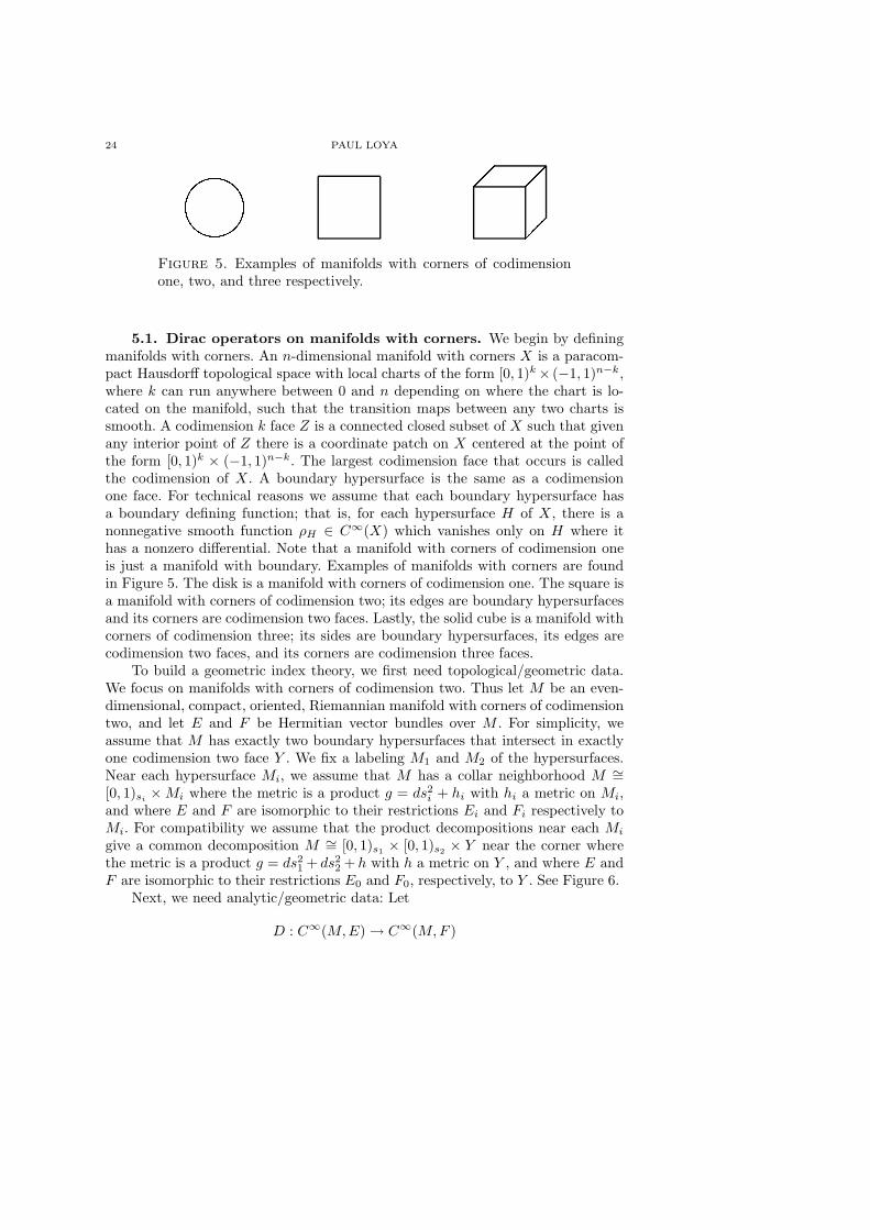
II
Figure 5. Examples of manifolds with corners of codimensionone, two, and three respectively.
5.1. Dirac operators on manifolds with corners. We begin by definingmanifolds with corners. An n-dimensional manifold with corners X is a paracom-pact Hausdorff topological space with local charts of the form [0, 1)k × (−1, 1)n−k,where k can run anywhere between 0 and n depending on where the chart is lo-cated on the manifold, such that the transition maps between any two charts issmooth. A codimension k face Z is a connected closed subset of X such that givenany interior point of Z there is a coordinate patch on X centered at the point ofthe form [0, 1)k × (−1, 1)n−k. The largest codimension face that occurs is calledthe codimension of X. A boundary hypersurface is the same as a codimensionone face. For technical reasons we assume that each boundary hypersurface hasa boundary defining function; that is, for each hypersurface H of X, there is anonnegative smooth function ρH ∈ C∞(X) which vanishes only on H where ithas a nonzero differential. Note that a manifold with corners of codimension oneis just a manifold with boundary. Examples of manifolds with corners are foundin Figure 5. The disk is a manifold with corners of codimension one. The square isa manifold with corners of codimension two; its edges are boundary hypersurfacesand its corners are codimension two faces. Lastly, the solid cube is a manifold withcorners of codimension three; its sides are boundary hypersurfaces, its edges arecodimension two faces, and its corners are codimension three faces.
To build a geometric index theory, we first need topological/geometric data.We focus on manifolds with corners of codimension two. Thus let M be an even-dimensional, compact, oriented, Riemannian manifold with corners of codimensiontwo, and let E and F be Hermitian vector bundles over M . For simplicity, weassume that M has exactly two boundary hypersurfaces that intersect in exactlyone codimension two face Y . We fix a labeling M1 and M2 of the hypersurfaces.Near each hypersurface Mi, we assume that M has a collar neighborhood M ∼=[0, 1)si
× Mi where the metric is a product g = ds2i + hi with hi a metric on Mi,
and where E and F are isomorphic to their restrictions Ei and Fi respectively toMi. For compatibility we assume that the product decompositions near each Mi
give a common decomposition M ∼= [0, 1)s1× [0, 1)s2
× Y near the corner wherethe metric is a product g = ds2
1 + ds22 + h with h a metric on Y , and where E and
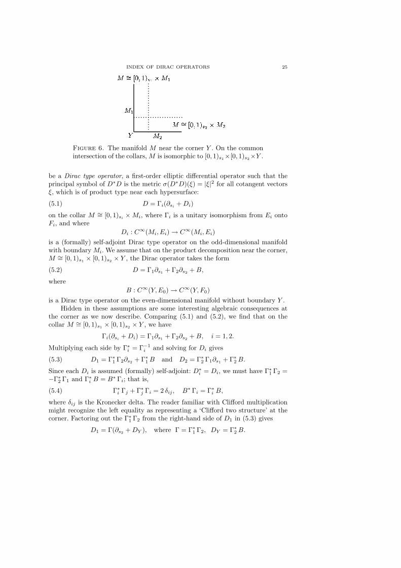
F are isomorphic to their restrictions E0 and F0, respectively, to Y . See Figure 6.Next, we need analytic/geometric data: Let
D : C∞(M,E) → C∞(M,F )
INDEX OF DIRAC OPERATORS 25
JK
JLM
J NO PQ R STUV W J K
J NO PQ R STUX W J L
Figure 6. The manifold M near the corner Y . On the commonintersection of the collars, M is isomorphic to [0, 1)s1
×[0, 1)s2×Y .
be a Dirac type operator, a first-order elliptic differential operator such that theprincipal symbol of D∗D is the metric σ(D∗D)(ξ) = |ξ|2 for all cotangent vectorsξ, which is of product type near each hypersurface:
(5.1) D = Γi(∂si+ Di)
on the collar M ∼= [0, 1)si× Mi, where Γi is a unitary isomorphism from Ei onto
Fi, and where
Di : C∞(Mi, Ei) → C∞(Mi, Ei)
is a (formally) self-adjoint Dirac type operator on the odd-dimensional manifoldwith boundary Mi. We assume that on the product decomposition near the corner,M ∼= [0, 1)s1
× [0, 1)s2× Y , the Dirac operator takes the form
(5.2) D = Γ1∂s1+ Γ2∂s2
+ B,
where
B : C∞(Y,E0) → C∞(Y, F0)
is a Dirac type operator on the even-dimensional manifold without boundary Y .Hidden in these assumptions are some interesting algebraic consequences at
the corner as we now describe. Comparing (5.1) and (5.2), we find that on thecollar M ∼= [0, 1)s1
× [0, 1)s2× Y , we have
Γi(∂si+ Di) = Γ1∂s1
+ Γ2∂s2+ B, i = 1, 2.
Multiplying each side by Γ∗i = Γ−1
i and solving for Di gives
(5.3) D1 = Γ∗1 Γ2∂s2
+ Γ∗1 B and D2 = Γ∗
2 Γ1∂s1+ Γ∗
2 B.
Since each Di is assumed (formally) self-adjoint: D∗i = Di, we must have Γ∗
1 Γ2 =−Γ∗
2 Γ1 and Γ∗i B = B∗ Γi; that is,
(5.4) Γ∗i Γj + Γ∗
j Γi = 2 δij , B∗ Γi = Γ∗i B,
where δij is the Kronecker delta. The reader familiar with Clifford multiplicationmight recognize the left equality as representing a ‘Clifford two structure’ at thecorner. Factoring out the Γ∗
1 Γ2 from the right-hand side of D1 in (5.3) gives
D1 = Γ(∂s2+ DY ), where Γ = Γ∗
1 Γ2, DY = Γ∗2 B.
26 PAUL LOYA
We call DY the induced Dirac operator on Y . We really should call DY the inducedoperator from D1. However, the induced operator from D2 is related to DY in asimple way. Indeed, one can verify that
D2 = −Γ(∂s1+ DY ), DY = ΓDY .
The induced Dirac operator on Y refers only to DY and not DY .As part of the ‘Clifford two package’, the induced operator DY has a nice
splitting property as we now describe. First, the left-hand identity in (5.4) impliesthat
Γ2 = −Id.
Hence, Γ : E0 → E0 has eigenvalues ±i. Let E±0 denote the eigenspaces corre-
sponding to the eigenvalues ±i; these are subbundles of E0 and
E0 = E+0 ⊕ E−
0
is an orthogonal decomposition since Γ is unitary. Also, a short computation uti-lizing (5.4) gives
DY Γ = −ΓDY .
Thus DY is odd with respect to Γ; hence odd with respect to the Z2-gradingE0 = E+
0 ⊕ E−0 . We summarize this property in the following lemma.
Lemma 5.1. With respect to the orthogonal decomposition E0 = E+0 ⊕ E−
0 ,where E±
0 are the ±i eigenspaces of Γ = Γ∗1 Γ2, the induced Dirac operator DY =
Γ∗2 B takes the following form
[0 D−
Y
D+Y 0
]: C∞(Y,E+
0 ⊕ E−0 ) → C∞(Y,E+
0 ⊕ E−0 ),
where D±Y are the restrictions of DY to C∞(Y,E±
0 ).
Note that since DY is self-adjoint, we have (D+Y )∗ = D−
Y . The following the-orem follows from the cobordism theorem of Atiyah-Singer, which is published inPalais’ book [69]. The cobordism theorem was one of the key steps in the originalproof of the Atiyah-Singer index theorem [6].
Theorem 5.2. The index of the Dirac type operator
D+Y : H1(Y,E+
0 ) → L2(Y,E−0 )
on the even-dimensional manifold without boundary Y is zero: indD+Y = 0. Since
(D+Y )∗ = D−
Y , it follows that dim kerD+Y = dim kerD−
Y .
5.2. Attaching multi-cylindrical ends. As in the manifold with boundarycase, we cannot build an index theory of D with its natural domain on the manifoldwith corners M :
Theorem 5.3. The Dirac type operator
D : H1(M,E) → L2(M,F )
is never Fredholm. In fact, dim kerD = ∞.
INDEX OF DIRAC OPERATORS 27
YZ
Y[\
]^ _ `abc d Y Z
]^ _ `abe d Y [
fgh _ ^ibe d Y [
fgh _ ^ibc d Y Z
fgh _ ^ibc d fgh _ ^ibe d \
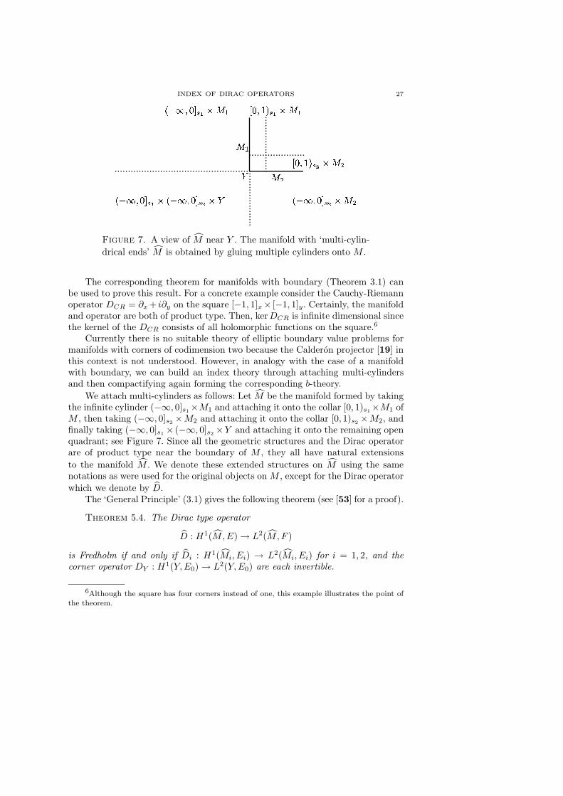
Figure 7. A view of M near Y . The manifold with ‘multi-cylin-
drical ends’ M is obtained by gluing multiple cylinders onto M .
The corresponding theorem for manifolds with boundary (Theorem 3.1) canbe used to prove this result. For a concrete example consider the Cauchy-Riemannoperator DCR = ∂x + i∂y on the square [−1, 1]x × [−1, 1]y. Certainly, the manifoldand operator are both of product type. Then, kerDCR is infinite dimensional sincethe kernel of the DCR consists of all holomorphic functions on the square.6
Currently there is no suitable theory of elliptic boundary value problems formanifolds with corners of codimension two because the Calderon projector [19] inthis context is not understood. However, in analogy with the case of a manifoldwith boundary, we can build an index theory through attaching multi-cylindersand then compactifying again forming the corresponding b-theory.
We attach multi-cylinders as follows: Let M be the manifold formed by takingthe infinite cylinder (−∞, 0]s1
×M1 and attaching it onto the collar [0, 1)s1×M1 of
M , then taking (−∞, 0]s2×M2 and attaching it onto the collar [0, 1)s2
×M2, andfinally taking (−∞, 0]s1
× (−∞, 0]s2×Y and attaching it onto the remaining open
quadrant; see Figure 7. Since all the geometric structures and the Dirac operatorare of product type near the boundary of M , they all have natural extensions
to the manifold M . We denote these extended structures on M using the samenotations as were used for the original objects on M , except for the Dirac operator
which we denote by D.The ‘General Principle’ (3.1) gives the following theorem (see [53] for a proof).
Theorem 5.4. The Dirac type operator
D : H1(M,E) → L2(M, F )
is Fredholm if and only if Di : H1(Mi, Ei) → L2(Mi, Ei) for i = 1, 2, and thecorner operator DY : H1(Y,E0) → L2(Y,E0) are each invertible.
6Although the square has four corners instead of one, this example illustrates the point of
the theorem.
28 PAUL LOYA
Here, Mi is the manifold with cylindrical end formed by attaching an infinite
cylinder to the odd-dimensional compact manifold with boundary Mi, and Di is
the natural extension of the Dirac operator Di to Mi.From Theorem 3.3, we know that the Dirac operator on a manifold with
a cylindrical end formed from a manifold with boundary can always be madeFredholm by considering it on weighted Sobolev spaces. For a manifold with cornersof codimension two, this is not the case.
Theorem 5.5. There exists a δ > 0 such that for all 0 < |α| < δ, the Diractype operator
D : eαsH1(M,E) → eαsL2(M, F )
is Fredholm if and only if the corner operator DY : H1(Y,E0) → L2(Y,E0) isinvertible (has zero kernel).
See [53] or [52] for a proof. Here, each coordinate function si is extended into
the rest of M to be a positive bounded function there, α = (α1, α2) is a pairof real numbers, 0 < |α| < δ means that 0 < |αi| < δ for i = 1, 2, and finally,eαs = eα1s1 eα2s2 . We remark that in many cases the kernels of Dirac operatorsrepresent topological quantities. In these cases, the invertibility of the corner Diracoperator would require certain cohomology groups of the corner Y to vanish. Thusthe Fredholm condition in Theorem 5.5 is actually very restrictive.
5.3. Muller’s generalization of the APS index formula. We now ex-plain Muller’s generalization [67] of the APS formula in Theorem 3.4 to manifoldswith corners of codimension two under the assumption that the corner Dirac op-erator DY is invertible. We remove this assumption in Section 6.
We first need to introduce the b-eta invariants of the operators D1 and D2,
cf. [59, Sec. 9.7]. Consider the operator D1 on M1. Here, M1 is the manifold withcylindrical end formed by attaching an infinite cylinder to the odd-dimensional
compact manifold with boundary M1. The operator D1 turns out to have contin-
uous spectrum, and not discrete spectrum, due to the fact that M1 has infinitevolume. Thus its eta invariant cannot be defined as a regularized signature in thesame way as in the case of a manifold with boundary considered in Section 3.2.
However, since the heat operator of D21 does exist, we can still try to define the
eta invariant via the integral (3.3):
“ η(D1) =1√π
∫ ∞
0
t−1/2 Tr(D1 e−tD21 ) dt ”.
Unfortunately, the operator D1 e−tD21 is not trace class, cf. Section 4.3, so the
right-hand side is not defined, which is the reason for the quotes. However, the
b-trace of D1 e−tD21 is defined.7 Replacing Tr with bTr in the above formula defines
7We first compactify M1, and then define the b-trace as in Section 4.3.
INDEX OF DIRAC OPERATORS 29
the b-eta invariant8,
bη(D1) =1√π
∫ ∞
0
t−1/2 bTr(D1 e−tD21 ) dt.
The b-eta invariant of D2 is defined in the same way. The APS formula in Theo-rem 3.4 generalizes as follows.
Theorem 5.6 (Muller, 1996). Let D be a Dirac type operator on an even-dimensional, compact, oriented, Riemannian manifold with corners of codimensiontwo with exactly two boundary hypersurfaces intersecting in exactly one corner andwith product type structures specified. Then there exists a δ > 0 such that for all0 < |α| < δ, the Dirac type operator
D : eαsH1(M,E) → eαsL2(M, F )
is Fredholm if and only if the corner operator DY : H1(Y,E0) → L2(Y,E0) isinvertible (has zero kernel); in which case,
indα D =
∫
M
KAS − 1
2
∑
i=1,2
{bη(Di) + sign α · dim ker Di
}.
Muller’s theorem in [67] technically only applies to the case of α > 0; in thegenerality presented above, the theorem is due to Melrose, cf. [53]. The formula
for indα D is almost exactly the same as the APS formula in Theorem 3.4. In fact,using the b-calculus, the proof of Theorem 5.6 proceeds in almost identical fashionas the proof of Theorem 3.4. The only ‘hard’ part is defining the appropriategeneralization of b-pseudodifferential operators and the b-trace to manifolds withcorners of codimension two. Once this machinery is set up, the proof of the APSindex formula can be used to prove Theorem 5.6.
5.4. b-version of Muller’s theorem. In analogy with the case of a mani-
fold with boundary, we now compactify the manifold M by introducing the changeof variables x1 = es1 and x2 = es2 . As si → −∞, xi → 0, and so this change of
variables compactifies M to be the interior of a compact manifold with cornersof codimension two, which we denote by X. Moreover, since dsi = dxi/xi and
∂si= xi∂xi
, the geometric objects on M transform into corresponding singulargeometric ‘b-objects’ on the compact manifold with corners:
g = ds21 + ds2
2 + h g =(dx1
x1
)2
+(dx2
x2
)2
+ h (b-metric),
dg = ds1 ds2 dh dg =dx1
x1
dx2
x2dh (b-measure),
Hk(M) Hkb (X) (b-Sobolev space),
8The same discussion as in footnote (4) concerning the local index theorem on odd-
dimensional manifolds without boundary applies in this situation too.
30 PAUL LOYA
and finally,
D = Γ1∂s1+ Γ2∂s2
+ B D = Γ1 x1∂x1+ Γ2 x2∂x2
+ B,
a b-differential operator. We repeat the statement of Muller’s theorem in thepresent context.
Theorem 5.7. Let D be a Dirac type operator on an even-dimensional, com-pact, oriented, Riemannian manifold with corners of codimension two with exactlytwo boundary hypersurfaces intersecting in exactly one corner and with producttype structures specified. Then there exists a δ > 0 such that for all 0 < |α| < δ,the Dirac type operator
D : xαH1b (X,E) → xαL2
b(X,F )
is Fredholm if and only if the corner operator DY : H1(Y,E0) → L2(Y,E0) isinvertible (has zero kernel); in which case,
indα D =
∫
M
KAS − 1
2
∑
i=1,2
{bη(Di) + sign α · dim ker Di
}.
As already mentioned, with a proper generalization of b-pseudodifferential op-erators and the b-trace to manifolds with corners of codimension two, the proof ofTheorem 5.7 proceeds in almost identical fashion as the proof of Theorem 3.4. Infact, the above theorem and its proof generalize to not only Dirac type operatorsbut also b-pseudodifferential on manifolds with corners of arbitrary codimension(see [50, 51, 52, 53]). These generalizations are due to Melrose (for Dirac op-erators) and the author (for b-pseudodifferential operators), cf. Lauter and Mo-roianu [44] for the cusp case. The ability to handle arbitrary codimensions is anice feature of using b-pseudodifferential operators to attack index problems onmanifolds with corners.
5.5. Some remarks on index theory on manifolds with corners. In[75] Salomenson builds an index theory for Dirac operators on manifolds withcorners of codimension two by attaching cylinders in a very different way thanconsidered here. Instead of attaching separate cylinders to each hypersurface Mi
and then filling in the lower quadrant with a product cylinder as shown in Fig-ure 7, he notes that ∂M has a natural smooth structure and attaches the cylinder(−∞, 0] × ∂M onto M . This creates a manifold with cylindrical end like in thecase of a manifold with boundary, except that it has a ‘wedge singularity’ at theoriginal corner Y . Results of Cheeger [22] or Chou [24] can be used to handle thewedge singularity.
In a different direction, Hassel, Mazzeo, and Melrose [41] prove a signatureformula for manifolds with corners of codimension two. Unlike the signature formu-las for manifolds with and without boundary, which are direct corollaries of indexformulas on such manifolds, the HMM formula is not a consequence of an indexformula on manifolds with corners of codimension two. Instead, they round off thecorner and consider X as a limit as ε → 0 of manifolds with smooth boundary Xε.
INDEX OF DIRAC OPERATORS 31
The resulting signature formula is obtained by a careful analysis of the limit of theAPS signature formulas of each Xε. They rely on ‘analytic surgery’ techniques in[40] to identify the limiting formula. Wall [84] considers a manifold with boundarydivided into two parts, each a manifold with corners of codimension two (e.g., adisk divided into two half wedges). Although not an index formula per se, Wallgives a formula for the signature of the manifold with boundary in terms of thesignatures of the two manifolds with corners of codimension two and a correctionterm given by the Maslov index of certain Lagrangian subspaces, cf. Section 6.
6. Perturbations of Dirac operators on manifolds with corners
We now consider the APS index formula for manifolds with corners of codi-mension two dropping the invertibility assumption on the corner Dirac operator.From our experience with the Gauss-Bonnet formula in the introduction, we expectthere to be a correction term added to the right-hand side of the APS formula dueto the presence of the corners. Theorem 5.6 did not have a corner contribution,essentially because the invertibility of the corner Dirac operator DY makes the
Dirac operator D not ‘notice’ the presence of the corners. For the Gauss-Bonnetformula, the correction term was given by the exterior angles of the corners. Forthe APS formula without the invertibility assumption on the corner operator, thereis a correction term in the index formula and it represents an ‘exterior angle’ ofsorts between certain Lagrangian vector spaces. In this section, we use the samenotation as in Section 5.
6.1. Fredholm perturbation of Dirac operators. By Theorem 5.5, thereexists a δ > 0 such that for all 0 < |α| < δ, the Dirac type operator
D : xαH1b (X,E) → xαL2
b(X,F )
is Fredholm if and only if the corner operator DY : H1(Y,E0) → L2(Y,E0) is in-vertible (has zero kernel). This nondegeneracy condition is actually very restrictivesince in many cases the kernels of Dirac operators represent cohomology. However,
we now show that it is always possible to make D Fredholm on weighted Sobolevspaces by perturbation with b-smoothing operators.
To define these perturbations we recall some notation from Section 5.1. Themanifold with corners of codimension two M is assumed to have exactly two bound-ary hypersurfaces M1 and M2 that intersect in exactly one codimension two faceY . Near the corner Y the Dirac type operator D takes the form
D = Γ1∂s1+ Γ2∂s2
+ B,
where
B : C∞(Y,E0) → C∞(Y, F0)
is a Dirac type operator on the even-dimensional manifold without boundary Y .The induced operator D1 on the hypersurface M1 takes the form
(6.1) D1 = Γ(∂s2+ DY ), Γ = Γ∗
1 Γ2, DY = Γ∗2 B,
32 PAUL LOYA
and the operator D2 on M2 takes the form
(6.2) D2 = −Γ(∂s1+ DY ), DY = ΓDY .
The minus sign in front of Γ and the fact that DY = ΓDY will come into playlater. Also, see Lemma 5.1, E0 = E+
0 ⊕ E−0 where E±
0 are the ±i eigenspaces ofΓ = Γ∗
1 Γ2, and the induced Dirac operator DY = Γ∗2 B is odd with respect to Γ
and so decomposes as[
0 D−Y
D+Y 0
]: C∞(Y,E+
0 ⊕ E−0 ) → C∞(Y,E+
0 ⊕ E−0 ),
where D±Y are the restrictions of DY to C∞(Y,E±
0 ). Moreover, see Theorem 5.2,
D+Y : H1(Y,E+
0 ) → L2(Y,E−0 )
has index zero; that is, dim kerD+Y = dim ker D−
Y .We now define the perturbations. Since the kernel of the Dirac type operator
DY is exactly the obstruction to D being Fredholm on weighted Sobolev spaces,the perturbations are chosen to be isomorphisms on the kernel. Since DY is oddwith respect to Γ, we only consider isomorphisms on ker DY having the sameproperty. Thus, let T : ker DY → ker DY be a self-adjoint unitary isomorphismthat is odd with respect to Γ. Hence T decomposes as an odd matrix
[0 T−
T+ 0
]: kerD+
Y ⊕ ker D−Y → ker D+
Y ⊕ ker D−Y ,
where T± : kerD±Y → ker D∓
Y are unitary isomorphisms with respect to theL2 inner product on kerDY ⊂ L2(Y,E0). Such an operator T exists becausedim ker D+
Y = dim kerD−Y . We can define T explicitly as follows. Let {uj}N
j=1
and {vj}Nj=1 be orthonormal bases of kerD+
Y and ker D−Y , respectively. By elliptic
regularity, uj , vj ∈ C∞(Y,E0) for every j. Then,
T =
N∑
j=1
uj ⊗ vj +
N∑
j=1
vj ⊗ uj
defines a self-adjoint unitary isomorphism on kerDY that is odd with respect toΓ and any such T can be written in this way for some choice of bases. Moreover,this formula shows that T is a smoothing operator on Y . Obviously,
DY − T : H1(Y,E0) → L2(Y,E0)
is invertible. This suggests that if we can extend T to an operator T on X, then
D − T : xαH1b (X,E) → xαL2
b(X,F )
is Fredholm for all 0 < |α| < δ for some δ > 0. To extend T , we first define T
on the manifold with multi-cylindrical ends M . Let χ ∈ C∞c ([0, 1)2) be such that
INDEX OF DIRAC OPERATORS 33
χ(x) = 1 for x near zero. Then χ(es) = χ(es1 , es2) can be regarded as a smooth
function on M supported on the cylindrical end (cf. Figure 7)
(−∞, 0]s1× (−∞, 0]s2
× Y.
Let ϕ(ξ1, ξ2) = e−ξ21−ξ2
2 . Then, given any u ∈ C∞c (M,E), we define
(6.3) T u(s, y) = χ(es) Γ21
(2π)2
∫
R2
eis·ξ ϕ(ξ)T χu(ξ, y) dξ,
where χu is the Fourier transform of χ(es)u(s, y) with respect to s:
χu(ξ, y) =1
(2π)2
∫
R2
e−is·ξ χ(es)u(s, y) ds.
The reason for the factor of Γ2 on the right-hand side of T u is that T is required tomap sections of E to sections of F and the Γ2 factor provides this property. Note
that the operator T in the definition of T only acts on the y variable of χu(ξ, y).Regarded as an operator on the compactified manifold X under the change of
variables xi = esi , the operator T is an example of a b-smoothing operator; thatis, a b-pseudodifferential operator of order −∞. The mapping properties of suchoperators (cf. [59, Ch. 5]) imply that
T : xαHkb (X,E) → xαH`
b(X,F ) for all α, k, `.
The next result follows from the properties of b-pseudodifferential operators andthe fact that DY − T : H1(Y,E0) → L2(Y,E0) is invertible, cf. [52, 53].
Lemma 6.1. There exists a δ > 0 such that for all 0 < |α| < δ,
D − T : xαH1b (X,E) → xαL2
b(X,F )
is Fredholm.
6.2. An index formula for perturbed Dirac operators. We now give a
formula for the index of D− T . Before doing so, we need to review the ‘scattering
Lagrangian’ of each operator Di. Consider the operator D1 on M1. Recall that M1
is formed by attaching an infinite cylinder (−∞, 0]s2× Y to the odd-dimensional
compact manifold with boundary M1. The set
ΛC1=
{lim
s2→−∞u(s2, y) ; u ∈ C∞(M1, E) is bounded, and D1u = 0
}
is called the scattering Lagrangian of D1. It turns out that ΛC1⊂ ker DY and the
dimension of ΛC1is exactly one-half the dimension of kerDY , cf. [59, Sec. 6.5]. The
scattering matrix of D1 is the operator C1 : kerDY → ker DY defined by C1 = +1on ΛC1
and C1 = −1 on Λ⊥C1
, where ‘⊥’ means the orthogonal complement with
respect to the L2 inner product. Then C1 is odd with respect to Γ, cf. [65, Sec. 4].
The scattering Lagrangian ΛC2and the matrix C2 of D2 are defined in the same
way. In [53] we give the following formula for the index of D − T :
34 PAUL LOYA
Theorem 6.2 (Loya-Melrose, 2002). Let D be a Dirac type operator on aneven-dimensional, compact, oriented, Riemannian manifold with corners of codi-mension two with exactly two boundary hypersurfaces intersecting in exactly onecorner and with product type structures specified. Let T : ker DY → ker DY be a
self-adjoint unitary isomorphism that is odd with respect to Γ and let T be the per-turbation defined by (6.3). Then there exists a δ > 0 such that for all 0 < |α| < δ,the perturbed Dirac operator
D − T : xαH1b (X,E) → xαL2
b(X,F )
is Fredholm. Moreover, if its index is denoted by indα(D − T ), then
indα(D − T ) =
∫
M
KAS − 1
2
∑
i=1,2
{bη(Di) + sign α · dim ker Di
}
− 1
2cα(ΛT ,ΛC1
,ΛC2).
(6.4)
The first line on the right-hand side is the same as in Theorem 5.7; the third‘corner correction term’ is described as follows. First, ΛT ⊂ ker DY is the +1eigenspace of the matrix T (since T is a self-adjoint unitary isomorphism, T 2 = Id,so T has eigenvalues ±1). Then,
(6.5) cα(ΛT ,ΛC1,ΛC2
) = sign α ·{
dim(ΛT ∩ ΛC1) + dim(ΛΓT ∩ ΛC2
)}
+ η(DG),
where ΛΓT ⊂ ker DY is the +1 eigenspace of the self-adjoint unitary isomorphismΓT and η(DG) is the eta invariant of a Dirac operator on a directed graph Gdefined as follows, cf. [41], [55], [20], [47]. This graph has two vertices v1 and v2
representing the hypersurfaces M1 and M2, respectively, and two edges e12 ande21 connecting the vertices representing the single corner Y . To put a manifoldstructure on this graph, we identify ejk with the interval [−1, 1]t, where the vertexvj corresponds to t = −1 and the vertex vk to t = +1. We consider V = kerDY ⊕ker DY as a ‘vector bundle’ over G where the first and second factors of kerDY
are ‘fibers’ over the edges e12 and e21, respectively. Thus a section of this vectorbundle is a sum s12 ⊕ s21, where sjk : ejk = [−1, 1] → ker DY . We define a Diracoperator DG acting on sections of G by
DG = Γd
dt⊕
(− Γ
d
dt
).
The minus sign in the second term stems from the minus sign in (6.2). The domainof DG consists of those sections s12 ⊕ s21 such that s12(v1) ∈ ΛT , s12(v2) ∈ ΛC1
,and s21(v2) ∈ ΛΓT , s21(v1) ∈ ΛC2
. The Lagrangian ΛΓT paired with the scattering
Lagrangian ΛC2stems from the fact that DY = ΓDY in (6.2). The term η(DG)
appearing in (6.5) is then the eta invariant of DG .Lesch and Wojciechowski [47] give the following linear-algebraic form for the
eta term:
η(DG) = m(ΛT ,ΛC1) − m(ΛΓT ,ΛC2
),
INDEX OF DIRAC OPERATORS 35
where
m(ΛL1,ΛL2
) = − 1
iπ
∑
eiθ∈spec(−L−
1L+
2)
θ∈(−π,π)
iθ
for any given self-adjoint unitary isomorphisms L1, L2 on ker DY that are oddwith respect to Γ, and with ΛLi
⊂ ker DY denoting the +1 eigenspace of Li. Thenumber m(ΛL1
,ΛL2) can be interpreted as an ‘exterior angle’ of sorts between ΛL1
and ΛL2, cf. [48], [20], [18]. Hassel, Mazzeo, and Melrose [40, 41] give a somewhat
more sophisticated linear-algebraic description of the eta term.Theorem 6.2 is proved as follows: First, following the proof of Theorem 5.7,
which uses similar arguments found in Section 4, produces the formula
indα(D − T ) =
∫
M
KAS − 1
2
∑
i=1,2
{bη(Di − Ti) + sign α · dim ker(Di − Ti)
},
where Ti is an operator naturally induced by T on Mi. The second and most
difficult part of the proof is to show that the terms involving Di − Ti in thisformula decompose as in (6.4). To do this, we show that
dim ker(Di − Ti) = dim ker Di + dim(ΛTi∩ ΛCi
),
where T1 = T and T2 = ΓT , and that
bη(Di − Ti) = bη(Di) ± m(ΛTi,ΛCi
),
where the sign is positive or negative if i = 1 or i = 2, respectively. The de-composition of the b-eta invariants uses techniques that have been developed bymany authors concerning gluing/splitting formulas for eta invariants, e.g. Bruningand Lesch [17] (cf. Vishik [83]), Douglas and Wojciechowski [28], Lesch and Wo-jciechowski [47], and Muller [65]. For related works on the eta invariant, seeSinger [80], Bunke [18], Dai and Freed [26], and Hassel, Mazzeo, and Melrose [40].
6.3. Some concluding remarks. If M has more than one corner, the resultfrom Theorem 6.2 still holds (with minor changes in the index formula accountingfor the various faces and corners) as long as we assume that each corner Diracoperator has index zero [53]. This assumption allows us to construct separate per-turbations for each corner, then sum these perturbations producing a b-smoothingoperator giving a Fredholm perturbation of the Dirac operator. Melrose and Nistorshow that it is in fact necessary that each corner operator have index zero for theexistence of a b-smoothing Fredholm perturbation. However, using a slightly largerclass of perturbations called ‘overblown’ b-smoothing operators, it is possible tomake Fredholm perturbations without any assumptions at the corners [54].
Current plans include relating the index of the perturbed Dirac operator toan index of the Dirac operator on a domain depending on the choice of perturba-tion. The index should be a type of Carron index [21]. In future work, we expectto generalize the program of ‘overblown’ b-smoothing Fredholm perturbations ofDirac operators to manifolds with corners of arbitrary codimension. Finally, one
36 PAUL LOYA
of the ultimate goals of this project is to derive via an index computation an an-alytic formula for the topological signature of any compact manifold with cornersof arbitrary codimension in terms of geometric and other types of invariants of themanifold and its boundary faces.
References
1. L. Alvarez-Gaume, Supersymmetry and the Atiyah-Singer index theorem, Comm. Math.
Phys. 90 (1983), no. 2, 161–173.
2. M. F. Atiyah, R. Bott, and V. K. Patodi, On the heat equation and the index theorem, Invent.
Math. 19 (1973), 279–330.
3. M. F. Atiyah, H. Donnelly, and I. M. Singer, Eta invariants, signature defects of cusps, and
values of L-functions, Ann. of Math. (2) 118 (1983), no. 1, 131–177.
4. M. F. Atiyah, V. K. Patodi, and I. M. Singer, Spectral asymmetry and Riemannian geometry,
Bull. London Math. Soc. 5 (1973), 229–234.
5. , Spectral asymmetry and Riemannian geometry. I, Math. Proc. Cambridge Philos.
Soc. 77 (1975), 43–69.6. M.F. Atiyah and I.M. Singer, The index of elliptic operators on compact manifolds, Bull.
Amer. Math. Soc. 69 (1963), 422–433.
7. , The index of elliptic operators I, Ann. Math. 87 (1968), 484–530.8. , The index of elliptic operators II, Ann. Math. 87 (1968), 531–545.9. N. Berline, E. Getzler, and M. Vergne, Heat kernels and Dirac operators, Springer-Verlag,
New York, 1992.
10. J.-M. Bismut and D.S. Freed, The analysis of elliptic families. II. Dirac operators, etainvariants, and the holonomy theorem, Comm. Math. Phys. 107 (1986), no. 1, 103–163.
11. J.-M. Bismut, The Atiyah-Singer index theorem for families of Dirac operators: two heatequation proofs, Invent. Math. 83 (1985), no. 1, 91–151.
12. J.-M. Bismut and J. Cheeger, Families index for manifolds with boundary, superconnections,and cones. I. Families of manifolds with boundary and Dirac operators, J. Funct. Anal. 89(1990), no. 2, 313–363.
13. , Families index for manifolds with boundary, superconnections and cones. II. The
Chern character, J. Funct. Anal. 90 (1990), no. 2, 306–354.14. B. Booss and D. D. Bleecker, Topology and analysis, Springer-Verlag, New York, 1985, The
Atiyah-Singer index formula and gauge-theoretic physics, Translated from the German by
Bleecker and A. Mader.15. B. Booß-Bavnbek and K. P. Wojciechowski, Elliptic boundary problems for Dirac operators,
Birkhauser Boston Inc., Boston, MA, 1993.16. J. Bruning, L2-index theorems on certain complete manifolds, J. Differential Geom. 32
(1990), no. 2, 491–532.17. J. Bruning and M. Lesch, On the η-invariant of certain nonlocal boundary value problems,
Duke Math. J. 96 (1999), no. 2, 425–468.
18. U. Bunke, On the gluing problem for the η-invariant, J. Differential Geom. 41 (1995), no. 2,397–448.
19. A.-P. Calderon, Boundary value problems for elliptic equations, Outlines Joint Sympos. Par-
tial Differential Equations (Novosibirsk, 1963), Acad. Sci. USSR Siberian Branch, Moscow,1963, pp. 303–304.
20. S. E. Cappell, R. Lee, and E. Y. Miller, On the Maslov index, Comm. Pure Appl. Math. 47(1994), no. 2, 121–186.
21. G. Carron, Theoremes de l’indice sur les varietes non-compactes, J. Reine Angew. Math.
541 (2001), 81–115.
22. J. Cheeger, Spectral geometry of singular Riemannian spaces, J. Differential Geom. 18
(1983), no. 4, 575–657 (1984).
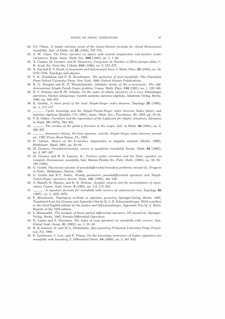
INDEX OF DIRAC OPERATORS 37
23. S.S. Chern, A simple intrinsic proof of the Gauss-Bonnet formula for closed Riemannian
manifolds, Ann. of Math. (2) 45 (1944), 747–752.
24. A. W. Chou, The Dirac operator on spaces with conical singularities and positive scalar
curvatures, Trans. Amer. Math. Soc. 289 (1985), no. 1, 1–40.
25. A. Connes, M. Gromov, and H. Moscovici, Conjecture de Novikov et fibres presque plats, C.
R. Acad. Sci. Paris Ser. I Math. 310 (1990), no. 5, 273–277.
26. X. Dai and D. S. Freed, η-invariants and determinant lines, J. Math. Phys. 35 (1994), no. 10,
5155–5194, Topology and physics.
27. S. K. Donaldson and P. B. Kronheimer, The geometry of four-manifolds, The Clarendon
Press Oxford University Press, New York, 1990, Oxford Science Publications.
28. R. G. Douglas and K. P. Wojciechowski, Adiabatic limits of the η-invariants. The odd-
dimensional Atiyah-Patodi-Singer problem, Comm. Math. Phys. 142 (1991), no. 1, 139–168.
29. B. V. Fedosov and B.-W. Schulze, On the index of elliptic operators on a cone, Schrodinger
operators, Markov semigroups, wavelet analysis, operator algebras, Akademie Verlag, Berlin,
1996, pp. 348–372.
30. E. Getzler, A short proof of the local Atiyah-Singer index theorem, Topology 25 (1986),
no. 1, 111–117.
31. , Cyclic homology and the Atiyah-Patodi-Singer index theorem, Index theory and
operator algebras (Boulder, CO, 1991), Amer. Math. Soc., Providence, RI, 1993, pp. 19–45.
32. P. B. Gilkey, Curvature and the eigenvalues of the Laplacian for elliptic complexes, Advances
in Math. 10 (1973), 344–382.
33. , The residue of the global η function at the origin, Adv. in Math. 40 (1981), no. 3,290–307.
34. , Invariance theory, the heat equation, and the Atiyah-Singer index theorem, second
ed., CRC Press, Boca Raton, FL, 1995.35. D. Grieser, Basics of the b-calculus, Approaches to singular analysis (Berlin, 1999),
Birkhauser, Basel, 2001, pp. 30–84.36. M. Gromov, Pseudoholomorphic curves in symplectic manifolds, Invent. Math. 82 (1985),
no. 2, 307–347.37. M. Gromov and H. B. Lawson, Jr., Positive scalar curvature and the Dirac operator on
complete Riemannian manifolds, Inst. Hautes Etudes Sci. Publ. Math. (1983), no. 58, 83–196 (1984).
38. G. Grubb, Functional calculus of pseudodifferential boundary problems, second ed., Progressin Math., Birkhauser, Boston, 1996.
39. G. Grubb and R.T. Seeley, Weakly parametric pseudodifferential operators and Atiyah-Patoti-Singer operators, Invent. Math. 121 (1995), 481–529.
40. A. Hassell, R. Mazzeo, and R. B. Melrose, Analytic surgery and the accumulation of eigen-values, Comm. Anal. Geom. 3 (1995), no. 1-2, 115–222.
41. , A signature formula for manifolds with corners of codimension two, Topology 36(1997), no. 5, 1055–1075.
42. F. Hirzebruch, Topological methods in algebraic geometry, Springer-Verlag, Berlin, 1995,
Translated from the German and Appendix One by R. L. E. Schwarzenberger, With a prefaceto the third English edition by the author and Schwarzenberger, Appendix Two by A. Borel,
Reprint of the 1978 edition.
43. L. Hormander, The analysis of linear partial differential operators. III, second ed., Springer-Verlag, Berlin, 1985, Pseudo-Differential Operators.
44. R. Lauter and S. Moroianu, The index of cusp operators on manifolds with corners, Ann.Global Anal. Geom. 21 (2002), no. 1, 31–49.
45. H. B. Lawson, Jr. and M.-L. Michelsohn, Spin geometry, Princeton University Press, Prince-
ton, NJ, 1989.
46. E. Leichtnam, J. Lott, and P. Piazza, On the homotopy invariance of higher signatures for
manifolds with boundary, J. Differential Geom. 54 (2000), no. 3, 561–633.
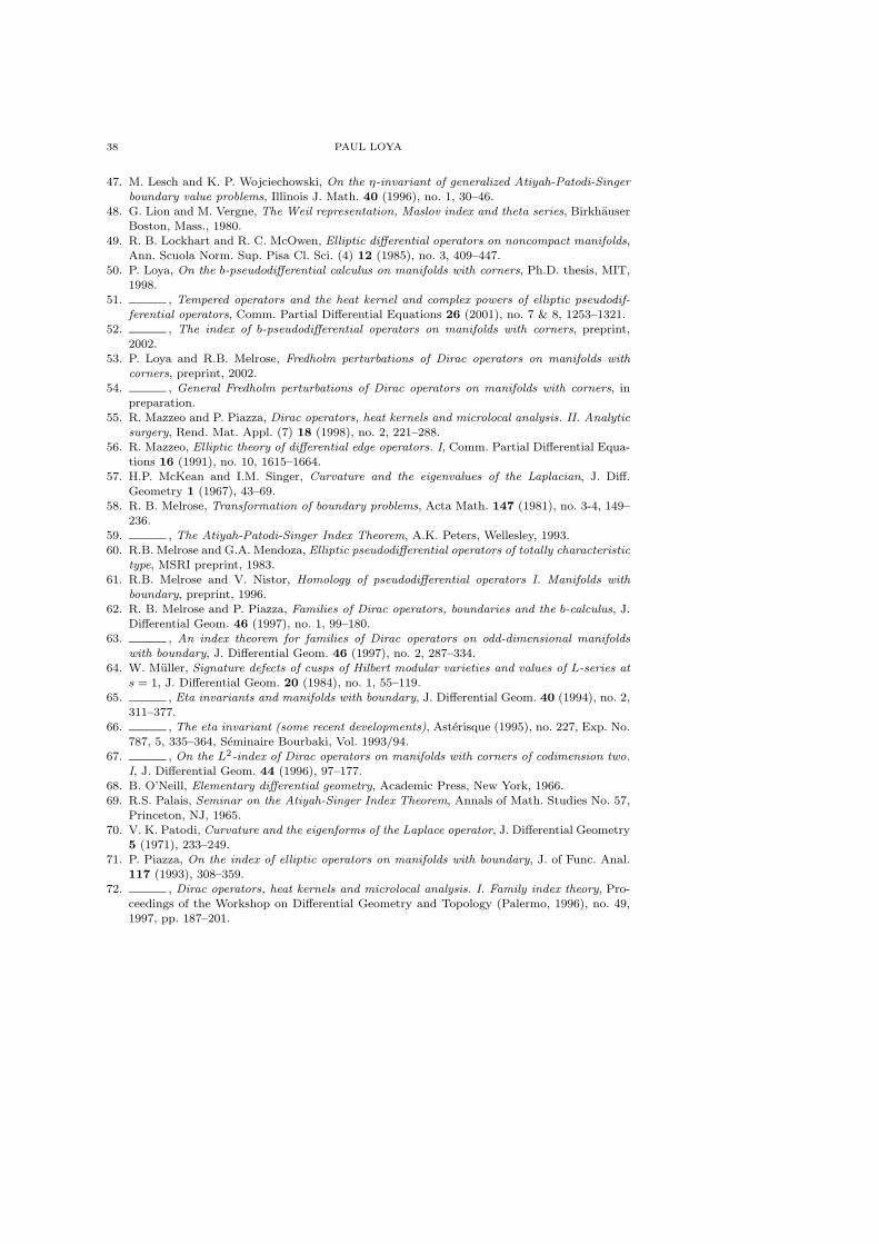
38 PAUL LOYA
47. M. Lesch and K. P. Wojciechowski, On the η-invariant of generalized Atiyah-Patodi-Singer
boundary value problems, Illinois J. Math. 40 (1996), no. 1, 30–46.
48. G. Lion and M. Vergne, The Weil representation, Maslov index and theta series, Birkhauser
Boston, Mass., 1980.
49. R. B. Lockhart and R. C. McOwen, Elliptic differential operators on noncompact manifolds,
Ann. Scuola Norm. Sup. Pisa Cl. Sci. (4) 12 (1985), no. 3, 409–447.
50. P. Loya, On the b-pseudodifferential calculus on manifolds with corners, Ph.D. thesis, MIT,
1998.
51. , Tempered operators and the heat kernel and complex powers of elliptic pseudodif-
ferential operators, Comm. Partial Differential Equations 26 (2001), no. 7 & 8, 1253–1321.
52. , The index of b-pseudodifferential operators on manifolds with corners, preprint,
2002.
53. P. Loya and R.B. Melrose, Fredholm perturbations of Dirac operators on manifolds with
corners, preprint, 2002.
54. , General Fredholm perturbations of Dirac operators on manifolds with corners, in
preparation.
55. R. Mazzeo and P. Piazza, Dirac operators, heat kernels and microlocal analysis. II. Analytic
surgery, Rend. Mat. Appl. (7) 18 (1998), no. 2, 221–288.
56. R. Mazzeo, Elliptic theory of differential edge operators. I, Comm. Partial Differential Equa-
tions 16 (1991), no. 10, 1615–1664.
57. H.P. McKean and I.M. Singer, Curvature and the eigenvalues of the Laplacian, J. Diff.
Geometry 1 (1967), 43–69.58. R. B. Melrose, Transformation of boundary problems, Acta Math. 147 (1981), no. 3-4, 149–
236.
59. , The Atiyah-Patodi-Singer Index Theorem, A.K. Peters, Wellesley, 1993.60. R.B. Melrose and G.A. Mendoza, Elliptic pseudodifferential operators of totally characteristic
type, MSRI preprint, 1983.61. R.B. Melrose and V. Nistor, Homology of pseudodifferential operators I. Manifolds with
boundary, preprint, 1996.62. R. B. Melrose and P. Piazza, Families of Dirac operators, boundaries and the b-calculus, J.
Differential Geom. 46 (1997), no. 1, 99–180.
63. , An index theorem for families of Dirac operators on odd-dimensional manifoldswith boundary, J. Differential Geom. 46 (1997), no. 2, 287–334.
64. W. Muller, Signature defects of cusps of Hilbert modular varieties and values of L-series ats = 1, J. Differential Geom. 20 (1984), no. 1, 55–119.
65. , Eta invariants and manifolds with boundary, J. Differential Geom. 40 (1994), no. 2,311–377.
66. , The eta invariant (some recent developments), Asterisque (1995), no. 227, Exp. No.787, 5, 335–364, Seminaire Bourbaki, Vol. 1993/94.
67. , On the L2-index of Dirac operators on manifolds with corners of codimension two.
I, J. Differential Geom. 44 (1996), 97–177.
68. B. O’Neill, Elementary differential geometry, Academic Press, New York, 1966.
69. R.S. Palais, Seminar on the Atiyah-Singer Index Theorem, Annals of Math. Studies No. 57,
Princeton, NJ, 1965.
70. V. K. Patodi, Curvature and the eigenforms of the Laplace operator, J. Differential Geometry5 (1971), 233–249.
71. P. Piazza, On the index of elliptic operators on manifolds with boundary, J. of Func. Anal.117 (1993), 308–359.
72. , Dirac operators, heat kernels and microlocal analysis. I. Family index theory, Pro-ceedings of the Workshop on Differential Geometry and Topology (Palermo, 1996), no. 49,
1997, pp. 187–201.
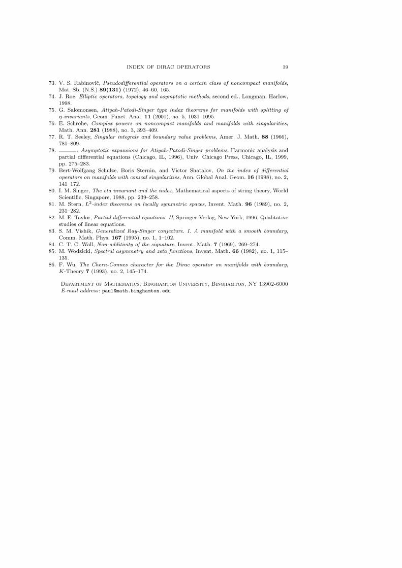
INDEX OF DIRAC OPERATORS 39
73. V. S. Rabinovic, Pseudodifferential operators on a certain class of noncompact manifolds,
Mat. Sb. (N.S.) 89(131) (1972), 46–60, 165.
74. J. Roe, Elliptic operators, topology and asymptotic methods, second ed., Longman, Harlow,
1998.
75. G. Salomonsen, Atiyah-Patodi-Singer type index theorems for manifolds with splitting of
η-invariants, Geom. Funct. Anal. 11 (2001), no. 5, 1031–1095.
76. E. Schrohe, Complex powers on noncompact manifolds and manifolds with singularities,
Math. Ann. 281 (1988), no. 3, 393–409.
77. R. T. Seeley, Singular integrals and boundary value problems, Amer. J. Math. 88 (1966),
781–809.
78. , Asymptotic expansions for Atiyah-Patodi-Singer problems, Harmonic analysis and
partial differential equations (Chicago, IL, 1996), Univ. Chicago Press, Chicago, IL, 1999,
pp. 275–283.
79. Bert-Wolfgang Schulze, Boris Sternin, and Victor Shatalov, On the index of differential
operators on manifolds with conical singularities, Ann. Global Anal. Geom. 16 (1998), no. 2,
141–172.
80. I. M. Singer, The eta invariant and the index, Mathematical aspects of string theory, World
Scientific, Singapore, 1988, pp. 239–258.
81. M. Stern, L2-index theorems on locally symmetric spaces, Invent. Math. 96 (1989), no. 2,
231–282.
82. M. E. Taylor, Partial differential equations. II, Springer-Verlag, New York, 1996, Qualitative
studies of linear equations.83. S. M. Vishik, Generalized Ray-Singer conjecture. I. A manifold with a smooth boundary,
Comm. Math. Phys. 167 (1995), no. 1, 1–102.
84. C. T. C. Wall, Non-additivity of the signature, Invent. Math. 7 (1969), 269–274.85. M. Wodzicki, Spectral asymmetry and zeta functions, Invent. Math. 66 (1982), no. 1, 115–
135.86. F. Wu, The Chern-Connes character for the Dirac operator on manifolds with boundary,
K-Theory 7 (1993), no. 2, 145–174.
Department of Mathematics, Binghamton University, Binghamton, NY 13902-6000
E-mail address: [email protected]


![REAL EMBEDDINGS AND THE ATIYAH-PATODI-SINGER INDEX THEOREM …€¦ · the Atiyah-Patodi-Singer index theorem for Dirac operators on manifolds with boundary [APS1]. Introduction](https://img.pdfslide.net/doc/110x75/5f0d06fb7e708231d43850e0/real-embeddings-and-the-atiyah-patodi-singer-index-theorem-the-atiyah-patodi-singer.jpg)