Embed Size (px)
Citation preview
Indian Statistical Institute
Asymptotic Theory for Some Families of Two-Sample Nonparametric StatisticsAuthor(s): Lars Holst and J. S. RaoSource: Sankhyā: The Indian Journal of Statistics, Series A, Vol. 42, No. 1/2 (Apr., 1980), pp.19-52Published by: Indian Statistical InstituteStable URL: http://www.jstor.org/stable/25050211Accessed: 18/06/2010 09:10
Your use of the JSTOR archive indicates your acceptance of JSTOR's Terms and Conditions of Use, available athttp://www.jstor.org/page/info/about/policies/terms.jsp. JSTOR's Terms and Conditions of Use provides, in part, that unlessyou have obtained prior permission, you may not download an entire issue of a journal or multiple copies of articles, and youmay use content in the JSTOR archive only for your personal, non-commercial use.
Please contact the publisher regarding any further use of this work. Publisher contact information may be obtained athttp://www.jstor.org/action/showPublisher?publisherCode=indstatinst.
Each copy of any part of a JSTOR transmission must contain the same copyright notice that appears on the screen or printedpage of such transmission.
JSTOR is a not-for-profit service that helps scholars, researchers, and students discover, use, and build upon a wide range ofcontent in a trusted digital archive. We use information technology and tools to increase productivity and facilitate new formsof scholarship. For more information about JSTOR, please contact [email protected].
Indian Statistical Institute is collaborating with JSTOR to digitize, preserve and extend access to Sankhy: TheIndian Journal of Statistics, Series A.
http://www.jstor.org
Sankhy? : The Indian Journal of Statistics
1980, Volume 42, Series A, Pts. 1 & 2, pp. 19-52.
ASYMPTOTIC THEORY FOR SOME FAMILIES OF
TWO-SAMPLE NONPARAMETRIC STATISTICS
By LARS HOLST*
University of Wisconsin, Madison and Uppsala University, Sweden
and
J. S. RAO
University of California, Santa Barbara, USA
SUMMARY. Let Xl9 ... , Xm-i and Ylt ... , Yn be independent random samples from
two continuous distribution functions F and O respectively on the real line. We wish to test
the null hypothesis that these two parent populations are identical. LetX' < ... ^ X'~ be
the ordered X-observations. Denote by Sjt the number of Y-observations falling in the interval
[X'v X'.), k = 1,... , m. This paper studies the asymptotic distribution theory and limiting
efficiencies of families of test statistics for the null hypothesis, based on these numbers {Sjt}. Let
h( . ) and {h*( . ) k = 1,. .. , m} be real-valued functions satisfying some simple regularity condi
tions. Asymptotic theory under the null hypothesis as well as under a suitable sequence of alter
m
natives, is studied for test statistics of the form 2 h(Sk), based symmetrically on $*'? and those fc-1
m of the form 2 hjc(Sjc) which are not symmetric in {Sjc}. It is shown here that tests of the symme
fc-1
trie type have poor asymptotic performance in the sense that they can only distinguish alter
natives at a "distance" of n"1^ from the hypothesis. Among this class of symmetric tests, which
includes for instance the well known run test and the Dixon test, it is shown that the Dixon
test has the maximum asymptotic relative efficiency. On the other hand, tests of the nonsym
metric type can distinguish alternatives converging at the more standard rate of n'112.
Wilcoxon-Mann-Whitney test is an example which belongs to this class. After investigating the
asymptotic theory under such alternatives, methods are suggested which allow one to select
m an "optimal" test against any specific alternative, from among tests of the type 2 hj?(Sjc).
*-=l
Connections with rank tests are briefly explored and some illustrative examples provided.
1. Introduction and notations
Let Xl9 ...,!,?_! and Yl9 ..., Yn be independent random samples from
two populations with continuous distribution functions (d.f.s.) F(x) and G(y)
respectively. We wish to test if these two populations are identical, i.e., the
hypothesis that the two d.f.s. are the same. A simple probability integral transformation carrying z->F(z) would permit us to assume that the support
Sponsored by the United States Army under Contract No, DAAG29-75-C-0024.
20 LARS HOLST AND J. S. RAO
of both the probability distributions is the unit interval [0, 1] and that the
first of them is the uniform d.f. on [0, 1], For the purposes of this discussion,
this probability transformation can be done without loss of any generality as
will be apparent soon. Thus from now on, we will assume that this reduction
has been effected and that the first sample is from the uniform distribution
?7(0, 1). Let G* = G o p-1 denote the d.f. of the second sample after the
probability transformation. The null hypothesis to be tested, specifies
HQ:G*(y) =
y, 0 < y < 1. ... (1.1)
Let 0 < Xi < ... < X'm_1 < 1 be the order statistics from the first sample. The sample spacings (Dv ..., Dm) for the X-values are defined by
Dk =
Dkm = X??X?_! , k=\, ...,m ... (1.2)
where we put X0 = 0 and X'm
? 1. Tests based on these sample spacings have been considered in the literature for the goodnesss-of-fit problems.
See for instance Darling (1953), Pyke (1965) and Rao and Sethuraman (1975). Define for k =
1, ..., m
Sk ? number of %'s
in the interval [X^_l5 X'k). ... (1.3)
Our aim is to study various test statistics based on these numbers {Sly .... Sm} for testing H0. These quantities may be called "spacing-frequencies" (since
they denote the frequencies of y's in the sample spacings of the x's) or the
"rank-spaeings" (since they correspond to the gaps in the ranks of the #'s in
the combined sample). Since the numbers {Sjc} as well as the statistics based
on them remain invariant under probability transformations, there is no loss of
generality in making such a transformation on the data, as was done earlier.
It may be remarked here that we take (m?1) instead of the usual m obser
vations in the first sample since this yields m numbers {Sv ..., Sm} instead of
(m+1), leading to slightly simpler notation. Tests based on {St} have been
considered for the two-sample problem in Dixon (1940), Godambe (1961) and
Rao (1976).
Our aim is to study the asymptotic theory as m and n tend to infinity. We will do this through a nondecreasing sequence of positive integers {mv}
and {nx] and assume throughout, that as v ?> oo,
mv ?? oo, nv ?> oo and mv/nv
= rv ?> p, 0 < p < oo. ...
(1.4)
Note that {Djc} defined in (1.2) depend on mv the number of X-values and it is
more appropriate to label them as {Dkv}. Similarly the numbers {$#} defined
TWO-SAMPLE NONPARAMETRIC STATISTICS 21
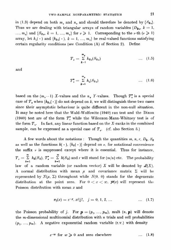
in (1.3) depend on both mv and nv and should therefore be denoted by {Skv}. Thus we are dealing with triangular arrays of random variables {Dky, k = 1,
..., mv} and {Skv, k ? 1, ..., mv} for v > 1. Corresponding to the v-th (v > 1)
array, let Av( ) and {A?v( ), k = 1, ..., rav} be real-valued functions satisfying certain regularity conditions (see Condition (A) of Section 2). Define
mv
?*v= Z A*V(S*V) ... (1.5) *=i
and
r;= s av(^v) ... (1.6)
fc-i
based on the (mv~l) X-values and the nv 7-values. Though T* is a special case of Tv when {hkv( )} do not depend on k, we will distinguish these two cases
since their asymptotic behaviour is quite different in the non-null situation.
It may be noted here that the Wald-Wolfowitz (1940) iun test and the Dixon
(1940) test are of the form T*v while the Wilcoxon-Mann-Whitney test is of
the form Tv. In fact, any linear function based on the X-ranks in the combined
sample, can be expressed as a special case of Tv. (cf. also Section 5.)
A few words about the notations : Though the quantities m, n, r, Dk, Sk as well as the functions A( ), {hk( )} depend on v, for notational convenience
the suffix v is suppressed except where it is essential. Thus for instance, m m
Tv = 2 hk(Sk), T*?
= S h(Sk) and r will stand for (m?n) etc. The probability fr=i *=?i
law of a random variable (or random vector) X will be denoted by <?(X). A normal distribution with mean ?i and covariance matrix S will be
represented by N(/i, S) throughout while N(0, 0) stands for the degenerate distribution at the point zero. For 0 < x < oo, p(x) will represent the
Poisson distribution with mean x and
7T^) =
e-*.^/j!, j = 0,1,2,... ... (1.7)
the Poisson probability of j. For p =
(pv ...,pm), mult (n, p) will denote
the m-dimensional multinomial distribution with n trials and cell probabilities
(Pv >Pm)' A negative exponential random variable (r.v.) with density
e~w for w ^ o and zero elsewhere (1.8)
22 LARS HOLST AND J. S. RAO
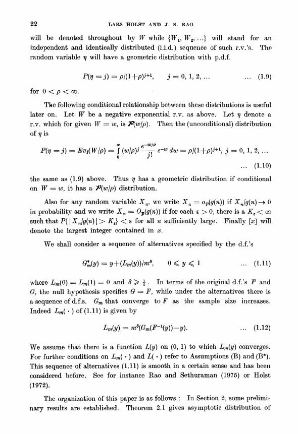
will be denoted throughout by W while {Wl7 W2, ...} will stand for an
independent and identically distributed (i.i.d.) sequence of such r.v.'s. The
random variable tj will have a geometric distribution with p.d.f.
Pfo=j)=p/(1+P)'+1, i = 0, 1,2, ... ... (1.9)
for 0 < p < oo.
The following conditional relationship between these distributions is useful
later on. Let IF be a negative exponential r.v. as above. Let r? denote a
r.v. which for given W = w, is 7?(w\p). Then the (unconditional) distribution
of 7j is
? f-W/P
P(v =
j) =
Err}(Wlp) =
J (w?p)S -^r- c~" dw =
p/(l+p)>+1, j = 0, 1, 2, ...
... (1.10)
the same as (1.9) above. Thus t? has a geometric distribution if conditional
on W = w, it has a ^(w/p) distribution.
Also for any random variable Xn, we write Xn =
op(g(n)) if XJg(n) ?> 0
in probability and we write Xn =
Op(g(n)) if for each e > 0, there is a Ks < oo
such that P{ | XJg(n) \ > Ke} < s for all n sufficiently large. Finally [x] will
denote the largest integer contained in x.
We shall consider a sequence of alternatives specified by the d.f.'s
GUV) = y+(Lm(y))lm*, 0 < y < 1 ... (1.11)
where Lm(0) =
Lm(l) = 0 and S > J . In terms of the original d.f.'s F and
C?, the null hypothesis specifies G = P, while under the alternatives there is
a sequence of d.f.s. Guthat converge to F as the sample size increases.
Indeed Lm( ) of (1.11) is given by
Lm(y) =
m*{Gm{F-\y))-y). ... (1.12)
We assume that there is a function L(y) on (0, 1) to which Lm(y) converges.
For further conditions on Lm( ) and L( ) refer to Assumptions (B) and (B*).
This sequence of alternatives (1.11) is smooth in a certain sense and has been
considered before. See for instance Rao and Sethuraman (1975) or Hoist
(1972).
The organization of this paper is as follows : In Section 2, some prelimi
nary results are established. Theorem 2.1 gives asymptotic distribution of

TWO-SAMPLE ttONfARAMEtRlC STATISTICS n
functions of multinomial frequencies while Theorem 2.2 establishes a result
on the limit distributions of non-symmetric spacings statistics, which is of
independent interest. These results are combined in Theorem 3.1 to obtain
the limit distribution of Ty under the alternatives (1.11) with S = |. It is
clear that putting Lm(y) == 0 in this theorem, gives the asymptotic distribution
of jTv under HQ. The problem of finding an asymptotically optimal test for
a given sequence of alternatives is considered in Theorem 3.2. Some specific
examples are discussed at the end of this section. Section 4 deals with the
symmetric statistics T*v. Theorem 4.1 gives the asymptotic distribution of
T\ under the sequence of alternatives (1.1) with 5= \ while Theorem 4.2
finds the optimal test among the symmetric tests. It is interesting to note
that symmetric classes of test statistics T\ can only distinguish alternatives
converging to the hypothesis at the slow rate of n 4 unlike the non-symmetric
statistics which can discriminate alternatives converging at the more usual _i
rate of n 2 . Similar results hold for tests based on sample spacings depend
ing on whether or not one considers symmetric statistics. See for instance
Rao and Sethuraman (1975) and Rao and Hoist (1980). Section 5 contains
some further remarks and discussion.
2. Some preliminary results
The following regularity conditions which limit the growth of the
functions as well as supply smoothness properties, will be needed for the
results of this and the next section.
Condition (A) : The real-valued functions {hk( )} defined on {0, 1, 2, ...}
satisfy Condition (A) if they are of the form
hk(j)^h(kl(m+l),j), *=l,...,w ? = 0,1,2,. (2.1)
for some function h(u, j) defined for 0 < u < 1, j = 0, 1, 2, ... with the
properties
(i) h(u,j) is continuous in u except for finitely many u and the
discontinuity set if any, does not depend onj.
(ii) h(u, j) is not of the form c >j+h(u) for some function A on [0, 1] and
a real number c.
(iii) For some d > 0, there exist constants c1 and c2 such that
IMn,j)| < cx [n(l-ii)]-i+S. (/2+l)
for all 0 < u < 1 and j = 0, 1, 2, ... ... (2.2)
24 LARS HOLST AND J. S. RA?
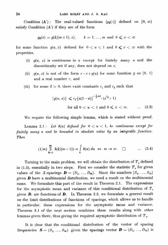
Condition (A') ; The real-valued functions {gjc(*)} defined on [0, oo)
satisfy Condition (A') if they are of the form
gic{x) ?
g(kl(m+l), x), k = 1, ..., m and 0 < x < oo
for some function g(u, x) defined for 0 < u < 1 and 0 <; x < oo with the
properties,
(i) g(u, x) is continuous in u except for finitely many u and the
discontinuity set if any, does not depend on x,
(ii) g(u, x) is not of the form c x-\-g(u) for some function g on [0, 1]
and a real number c, and
(iii) for some ? > 0, there exist constants cx and c2 such that
\g(u9x)\ < c^l-^f ?+^(a2+l)
for all 0 < u < 1 and 0 < x < oo. ... (2.3)
We require the following simple lemma, which is stated without proof.
Lemma 2.1 : Let h(u) defined for 0 < u < 1, be continuous except for
finitely many u and be bounded in absolute value by an integrable function.
Then
m i
(1/ra) 2 A(Jfc/(m+l))-> J h(u) du as ra-> oo. D (2-4) *=i o
Turning to the main problem, we will obtain the distribution of Tv defined
in (1.5), essentially in two steps. First we consider the statistic Tv for given
values of the X-spacings D = {Dv ..., Dm}. Since the numbers {Sv ..., Sm}
given D have a multinomial distribution, we need a result on the multinomial
sums. We formulate this part of the result in Theorem 2.1. The expressions
for the asymptotic mean and variance of this conditional distribution of Tv
given D, are functions of D. In Theorem 2.2, we formulate a general result
on the limit distributions of functions of spacings, which allows us to handle
in particular, these expressions for the asymptotic mean and variance.
Theorem 3.1 of the next section combines these results along with other
lemmas given there, thus giving the required asymptotic distribution of Ty.
It is clear that the conditional distribution of the vector of spacing
frequencies S = (Sv ..., Sm) given the spacings vector D =
(Dv ..., Dm) is
TWO-?AMPLE N?NPARAMETRI? STATISTICS 25
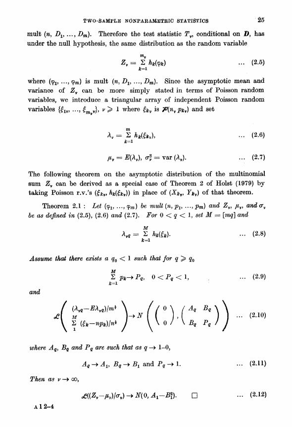
mult (n, Dv ..., Dm). Therefore the test statistic Ty9 conditional on D, has
under the null hypothesis, the same distribution as the random variable
mv
Zv = 2 hk(9k)
... (2.5) ?T=1
where (9^ ...,9^) is mult (n, Dv ...,Dm). Since the asymptotic mean and
variance of Zv can be more simply stated in terms of Poisson random
variables, we introduce a triangular array of independent Poisson random
variables {?lv, ..., gm v}, v > 1 where %kv is P(nvpkv) and set
m
Av= S hk(?kv), ... (2.6)
k=l
?iv =
E(Av), cr2 = var(Av).
... (2.7)
The following theorem on the asymptotic distribution of the multinomial
sum Zv can be derived as a special case of Theorem 2 of Hoist (1979) by
taking Poisson r.v.'s (?kv, hk(?kv)) in place of (Xky, Ykv) of that theorem.
Theorem 2.1 : Let (<pl5 ...,9^) be mult(n,pv ...,pm) and Zv, /iv, andav
be as defined in (2.5), (2.6) and (2.7). For 0 < q < 1, set M = [mq] and
M
Av,= 2 ?*(&). ... (2.8)
fc=i
Assume thai there exists a q0 < 1 such that for q > qQ
M 2 pk->Pq9 0<PQ<1,
... (2.9) k=l
and
where AQ, BQ and Pq are such that as q-+ 1-0,
Aa -> Ax, BQ -> ^ and Pa -> 1. ... (2.11)
TAew a?s j^ ?> 00,
^-^/^-?^OMx-u?. D ... (2.12)
A12-4
&6 ?LARS HOLST AND j. S. tlA?
From (2.6) and (2.7) an explicit expression for the mean is given by
/?v= 2 2 hk{j) ttj (npjc) ... (2.13) fc=l i=0
using the notation (1.7). Under the null hypothesis, we have pk = Dk,
k == 1, ..., m where D are the spacings from ?7(0, 1). Thus we consider
m ?
fi(nD) = p?nD) = S S ?*(j)*r,(nD*). ... (2.14) ?=l i=0
Wi oo
This is of the form 2 gjc{mDk) where (/?(a;) = 2 A?( j) 7r? (a:/r). k=i i=o
Statistics based on spacings have been considered earlier by Darling (1953), LeCam (1958), Pyke (1965) and Rao and Sethuraman (1975). Most of these
papers, however, discuss the symmetric case, i.e., when gk(x) =
g(x) for all k.
As Pyke (1965) pointed out (cf. Section 6.2), LeCam's method could be used
to study the more general non-symmetric case. Let {gk{ ), k = 1, ..., m} be real-valued measurable functions. For 0 < q < 1, let Mv
= [mv q].
Define
M
GQv= 2 gk(Wk) ... (2.15) fc=i
where {Wv W2, ...} is a sequence of i.i.d. exponential r.v.'s. Then the
following theorem states explicitly the asymptotic distribution of statistics
of the type (2.14) and is easily established by checking Assumption (6.6) of
Pyke (1965).
Theorem 2.2 : Assume that
0 < var (GQv) ==
o-2(Gqv) < oo for all q and v, ... (2.16)
and that for each q e (0, 1]
/ {Gqv-EG9v)l<r{Gu) \ / / 0 \ / At B9\\ M m ]^N[ ( ), ( ... (2.17) V S (F*-l)/m* j
V \ 0 / \ Bg q I J
with Aq and Bq such that
Aq-* Ax = 1 as tf->l-0 ... (2.18)
Ba -> Bx as q - 1-0. ... (2.19)
TWO-SAMPLE NONPARAMETRIC STATISTICS 27
Then, as v-^ oo,
??(( ?
gk(mDk)-EGlv'jl<r(Glv)) -> N(0, 1?J3J). ... (2.20)
wAere (Dv ..., Z>) are spacings from U(0, 1). Q
The following corollary gives a simple sufficient condition on the functions
gk( ) in order that the above Theorem holds.
Corollary 2.1 : The asymptotic normality asserted in Theorem 2.2 holds
for any set of functions {gk( )} which satisfy condition (A').
Proof : To prove this corollary, we need to check that the assumptions
(2.16) to (2.19) hold when condition (A') is satisfied. It can be easily checked
that if g(u, x) satisfies condition (A'), then
00 00 00
S 9?U> x)e~x dx, J g\u, x)e~x dx as well as J g(u, x)(x? l)e~x dx oo o
satisfy conditions of Lemma 2.1 in u. Thus from the definition of Gqv and
Lemma 2.1, as m ?? oo,
[mq] q
E(Gqv)lm = (Urn) 2 Eg(kl(m+1), Wk) -> J Eg(u, W) du ... (2.21)
k=i o
[mq] q var (Gqx)jm = (1/m) 2 var (g(kl(m+l),Wk)) -> J (var g(u, W)) du
k=i o
... (2.22) and
M [mq] cov (Gqv, 2 Wk)\m = (1/m) 2 cov (g(kl(m+l), Wk), Wk)
l k=l
~> J cov (g(u, W), W) du. ... (2.23) o
Again from (2.3) of condition (A'), all these limits are finite. These are also
continuous in q so that (2.18) and (2.19) are satisfied.
Finally to check the asymptotic normality in (2.17) or equivalently of
[ma] tm0l
S {a{gk{Wk)-Egk{Wic))+{Wle-\)}= S g*k(Wk), say ... (2.24) fc=i Jc=i
28 LARS HOLST AND J. S. RAO
for all real a, we have only to verify the Lindeberg condition for the non
identical case. It is easily seen that if {gk( )} satisfy condition (A'), so do
{gl( )} defined in (2.24). Let
(r? =
Eg\ (Wk) and sfm] = 2 erf. ... (2.25)
* k=l
Since {gl( )} satisfy condition (A'), we have as in (2.22) that
[mq] oo o
afmgI/? = (l/m)2 jg\(w)tr"?w
... (2.26) k=i o
converges to a finite non-zero constant from Lemma 2.1. Now consider
[mQ] 2
(i/^)s j 0;(*)6-*<fe
< (mlsfmq]) . dim) 2 J c1[(fc/(m+ i))(i_ t/(m+l)]-i+2'
(a;C2+l)2e-^da;
< {^/^?{(l/m) S [(?/(m+l))(l-i/(m+l))]-1+25} #=i
{ J (xe*+l)*e-*dx).
As m ?> oo, the quantities in the first two parentheses remain bounded because
of (2.26) and Lemma 2.1 while the integral in the third parenthesis goes to
zero for any e > 0 since s[mq^ is of order (\/m) from (2.26). Thus the Linde berg
condition is satisfied for (2.24) which proves the assertion.
3. Asymptotic distribution theory for
non-symmetric statistics
We define for later use, the following additional functions
00
gx(u, x) = 2 h(u, j) tt^x),
... (3.1)
00
g2(u, x) = 2 h2(u, j) tt} {x) ... (3.2)
and
g3(u, x) = 2 h(u,j)(j-x) n} (x). ... (3.3)
J-O
TWO-SAMPLE NONPARAMETRIC STATISTICS 29
When h(u, j) satisfies condition (A), these functions are well defined for x > 0.
Further gx and gr3 satisfy condition (A'). For instance condition (iii) of (A)
implies condition (iii) of (A') for gx since
I 00
\gx(u,x)\ = i 2 h(u,j)nj(x)
< SCiMl-ttjf^a+^^W ;=o
<c;Ml_w))-*+s(1+/2) _ (34)
using the moments of the Poisson distribution. To see the role of these
functions gv g2 and g3, recall the representation of r? given in (1.10). Let
Em Vw denote the expectation and variance over W while En?w Vn\W denote
the conditional expectation and variance over 7} given W. Then from the
definitions of gl9 g2, gz
Enh(u, ri) =
EwEnlw h(u, r/) =
Ewgi(u, W\p) ... (3.5)
Enh*(u, 7i) =
EwEn, w h\u, 7i) =
Ewg2(u, W/p). ... (3.6)
And after some elementary calculations,
P^+P)-1 COV (h(u, 7?), 7?) = EWEn]W [h(u, 7?)(7}- W/p)]
= cov(gi(u, W/p), W)
= Ew gs(u, W/p). ... (3.7)
Define
1 , 1 ,2
a-2 = j var ?^ ^ ?u__ j cov (h(Uj ̂ y) du /var (t?). ... (3.8) 0 \ o /
From the Cauchy-Schwartz inequality
/ 1 \2 , 1 i2
( J cov (A(w, 7/), ??) du J < f J (var h(u, 7/))*(var ?/)* dw 1
< var (t?) ( J* var A(w, 9/) dw ]
with equality if and only if h(u, j) = c j+h(u) for 0 < u < 1 for some real
number o and some function h(u). Thus a*2 > 0 for any function h(u,j)
satisfying condition (A). For x = (xv ..., xm), we define
?>v m co
/i(x) = fiv(x) = 2 g1(kl(m+l), xk) = 2 2 hk(j)nj(xk) ... (3.9) *=i *=i ;=o
and observe that /?(wD) corresponds to the statistic in (2.14).
30 LARS HOLST AND J. S. RAO
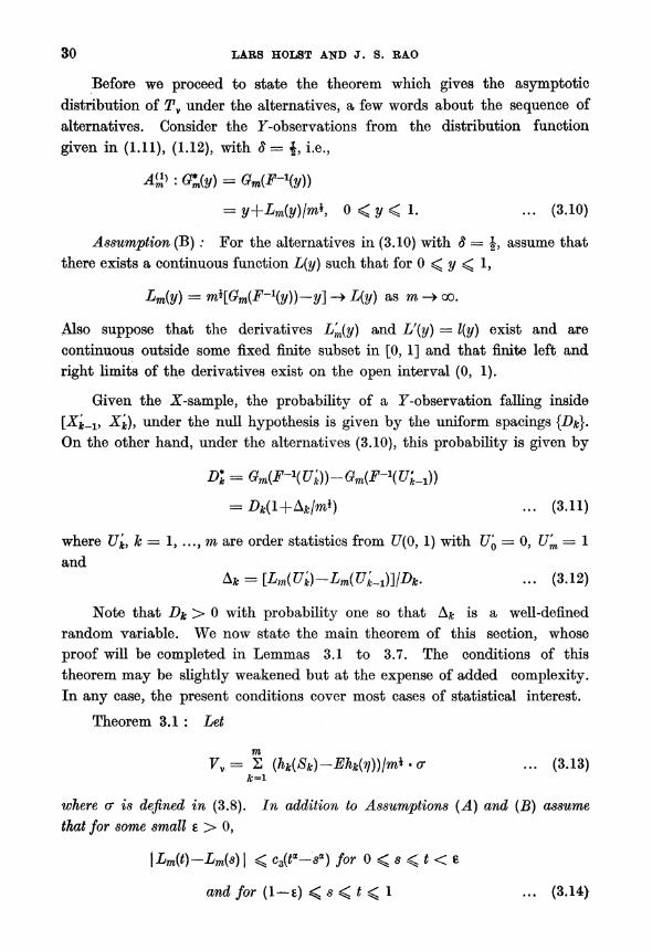
Before we proceed to state the theorem which gives the asymptotic
distribution of Tv under the alternatives, a few words about the sequence of
alternatives. Consider the F-observations from the distribution function
given in (1.11), (1.12), with S = i i.e.,
4?> : GUV) = Gm{F-\y))
= y+Lm(y)lmK 0 < y < 1. ... (3.10)
Assumption (B) ; For the alternatives in (3.10) with S = |, assume that
there exists a continuous function L(y) such that for 0 ^ y ^ 1,
Lm{y) =
m*[Gm(-F-%))?y] -> ?(y) as m -> oo.
Also suppose that the derivatives L'm(y) and L\y) =
%) exist and are
continuous outside some fixed finite subset in [0, 1] and that finite left and
right limits of the derivatives exist on the open interval (0, 1).
Given the X-sample, the probability of a F-observation falling inside
[Xk_v X?), under the null hypothesis is given by the uniform spacings {Dk}. On the other hand, under the alternatives (3.10), this probability is given by
DI = Gm{F-\U'k))-Gm{F-\UU))
= Z>*(l+A*/m*)
... (3.11)
where U'k, k = 1, ..., m are order statistics from ?7(0, 1) with U'0 = 0, U'm
= 1
and
Ak = [Lm(Uk)-Lm(U'k_1)]IDk. ... (3.12)
Note that Dk > 0 with probability one so that A*? is a well-defined
random variable. We now state the main theorem of this section, whose
proof will be completed in Lemmas 3.1 to 3.7. The conditions of this
theorem may be slightly weakened but at the expense of added complexity. In any case, the present conditions cover most cases of statistical interest.
Theorem 3.1 : Let
m
Vv = 2 (hk(Sk)-Ehk(V))lm*
- cr ... (3.13) k=l
where cr is defined in (3.8). In addition to Assumptions (A) and (B) assume
that for some small ? > 0,
\Lm(t)-Lm(s) | < c3(ia-5a) for 0 < s < t < 6
and for (1?e) < s < t <; 1 ... (3.14)
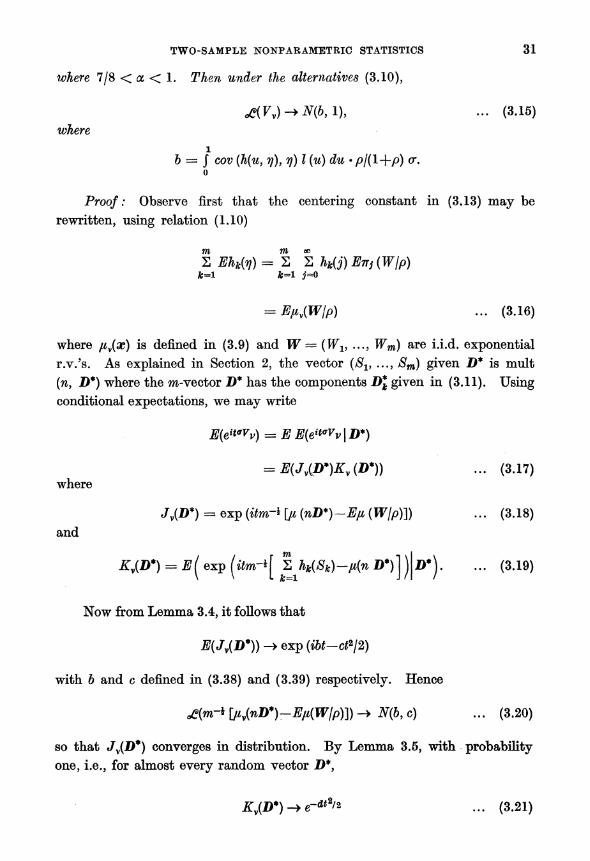
TWO-SAMPLE NONPARAMETRIC STATISTICS 31
where 7/8 < a < 1. Then under the alternatives (3.10),
?(Vy)->N(b,l), ... (3.15)
where
i b = J cov (h(u> 7?), 7j) l (u) du pl(l+p) c.
o
Proof : Observe first that the centering constant in (3.13) may be
rewritten, using relation (1.10)
m m ?
2 Ehk(7?)= 2 2 hk(3)E7?i(W?p) &=1 fc=l j=0
= Efiv(W?p) ... (3.16)
where ?iv(x) is defined in (3.9) and W = (Wl9 ..., Wm) are i.i.d. exponential
r.v.'s. As explained in Section 2, the vector (Sl9 ..., Sm) given D* is mult
(n, D*) where the m-vector D* has the components D\ given in (3.11). Using conditional expectations, we may write
E(e^vv) = E E(e^Vv\D*)
= E(Jv(iD*)Ky(D*)) ...
(3.17) where
JV(D*) = exp (itm-i \ji {nD*)-E/i (W?p)]) ... (3.18) and
KV(D*) = e(
exp (?im-i[
S hk(8k)-/i(n A*)] )|l>').
... (3.19)
Now from Lemma 3.4, it follows that
E{Jy(D*)) -> exp {ibt-ct2?2)
with 6 and c defined in (3.38) and (3.39) respectively. Hence
?(m-i[pv(nD*)-Eii(Wlp)])-> N(b,c) ... (3.20)
so that JV(D*) converges in distribution. By Lemma 3.5, with probability
one, i.e., for almost every random vector D*,
KV(D*) -> e-***'* (3.21)
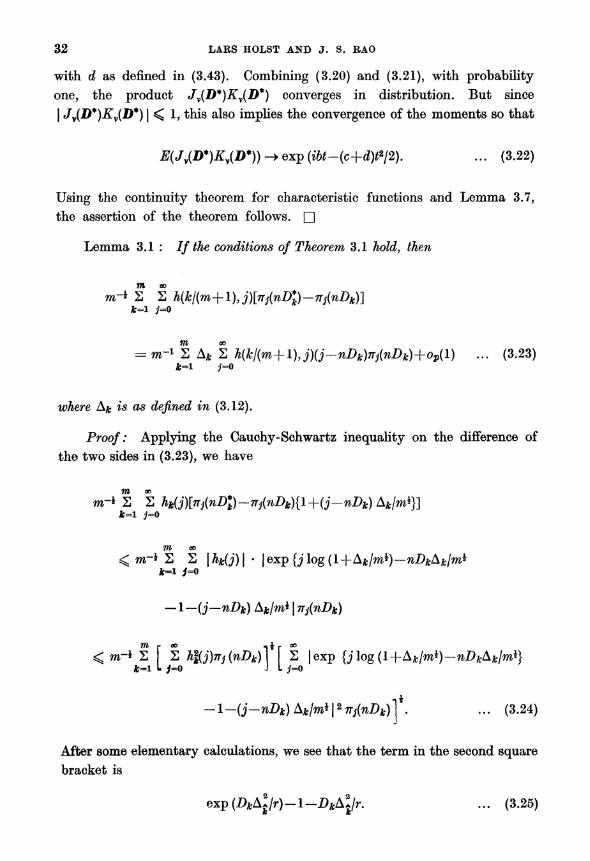
32 LARS HOLST AND J. S. RAO
with d as defined in (3.43). Combining (3.20) and (3.21), with probability one, the product JV(D*)KX(D*) converges in distribution. But since
| JV(D*)KV(D*) | < 1, this also implies the convergence of the moments so that
E(JV{D*)KV(D*)) -> exp (ibt-(c+d)t*?2). ... (3.22)
Using the continuity theorem for characteristic functions and Lemma 3.7,
the assertion of the theorem follows.
Lemma 3.1 : If the conditions of Theorem 3.1 hold, then
m-* 2 2 h(kl(m+l), j)Midfy-n?nDk)\ Ar=l ;=o
m oo = m-1 2 A* 2 h(kl(m+l),JXJ-nD^inD^+o^l) ... (3.23)
where Ak is as defined in (3.12).
Proof: Applying the Cauchy-Schwartz inequality on the difference of
the two sides in (3.23), we have
m~* 2 2 hU^inDD-n^nD^l+U-nDk) A*/m*}] *=i j=0
< m-* 2 2 \hfc(j)\ \exp{jlog(l+Aklmi)-nDkAklm* ifc=i j=o
? 1 -(j-nDk) Ak/m* \ 7Tj{nDk)
n~* 2 [ 2 h%j)7Tj {nDktf [ 2 |exp {jlog(l+Aklmi)-nDkAklm*}
^l^j^^^A^/m^l2^^)]*. ... (3.24)
After some elementary calculations, we see that the term in the second square
bracket is
exp (DkA?lr)-1 -D*A j/r. ... (3.25)
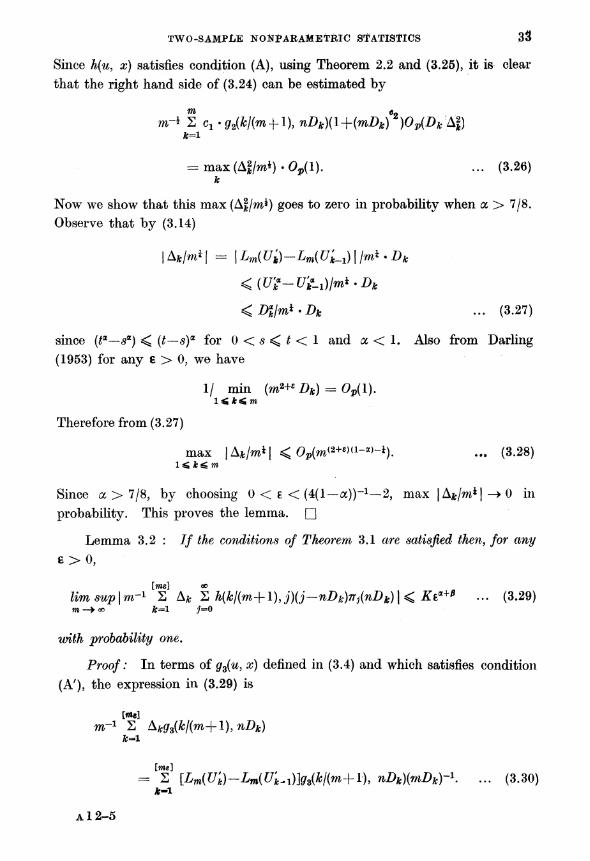
TWO-SAMPLE NONPARAMETRIC STATISTICS 33
Since h(u, x) satisfies condition (A), using Theorem 2.2 and (3.25), it is clear
that the right hand side of (3.24) can be estimated by
m-* 2 ^.^/(m + l^^Kl+im^)02^^^ ?=i
= max(Af/m*) Op(l).
... (3.26) k
Now we show that this max (Af/m*) goes to zero in probability when a > 7/8. Observe that by (3.14)
| A*/m* | = | Lm(Ui)-Lm(UU) I / * Dk
<(U?-U?L1)lm*-Dk
<D*klm*-Dk ... (3.27)
since (t*?sa) < (t?s)a for 0 < s < t < 1 and a < 1. Also from Darling
(1953) for any e > 0, we have
1/ min (m2+e Dk) = 0P(1).
Therefore from (3.27)
max lA^/m^l <O??(m(2+8>(1"a)-i). ... (3.28)
Since oc > 7/8, by choosing 0 < e < (4(1?a))-1?2, max |&k?m*\ -? 0 in
probability. This proves the lemma.
Lemma 3.2 : If the conditions of Theorem 3.1 are satisfied then, for any
?>0,
[me] oo
Urn sup?m-1 2 A* 2Hkl(m+l)9j)(j-nDk)n,(nI>k)\<Kta+? ... (3.29) m ?>oo k=l y=0
with probability one.
Proof : In terms of gs(u, x) defined in (3.4) and which satisfies condition
(A'), the expression in (3.29) is
[mc]
m-i 2 &kgz(kl(m+l),nDk) k=>i
[me] = 2 [Lm(Uk)~Lm(U'k^)]gz(kl(m+l), nDk)(rnDk)~\ ... (3.30)
A12-5
?4 LARS ?OLST ANt> J. ?. JEtA?
Using condition (3.14), and writing M = [mg], this is
0<
M 2 [LM)-Lm{U^x)] g8 (*/(m+l), it/)*) I (mD*)-1 i
< clCs 2 (J/?-?/?LiXfc/m^l+?AD*) 2]. ... (3.31) i
We now make use of the representation of the spacings in terms of i.i.d. ? k
exponential r.v.'s Wv W2, ... with mean 1. Writing Wk = 2 Wjjk, the
RHS in (3.31) is
cOH0 M _ _ _
?7 . A S [WtHk/M)?- W%^{{lc-l)IMYlklM)<>. (fl$+ W*) Wa+C2 1 rr m
= G - 6?+'. f^"*'2' if-1! ?Ff-i(*/Jf)?+'-i(?P?+1+ if? ^5)
'[{?-ii-wtik.wirymkwt)]. ... (3.32)
Now as k ?> 00, ?Fj; ?> 1 a.s. and Wk? ?> 0 a.s. so that
{1-(1- WklkWtf}HWtlkWt)-> a a.s. ... (3.33)
Using the Holder inequality,
~ |
Wr< (W+<->W?+' Rl-(1?WtlkWt)-)HWtllcW,)]
<[i?wr"p[?fwJo'**'] 1/JP,
Uf! J U, \ WkiikWje) H
n Using the fact that if ak
? 1 as k -? oo, w12 a? -? 1 as n -? oo, the RHS i
in (3.34) converges a.s. to the finite limit
TWO-SAMPLE NONPARAMETRIC STATISTICS 35
Similarly the other term involving Wk* W*? in (3.32) can be handled so that
we get the desired result. -Q
Lemma 3.3 : Under the conditions of Theorem 3.1,
m-1 2 &kgz(kl(m+l),nDk) k~i
l
?> J l(u) cov (h(u: 7j), 7j) du (pjl+p) in probability. ... (3.35) o
Proof : For any fixed e > 0, we may consider the sum in (3.35) as Consist ?e] [m(l-e)] m
ing of 3 parts viz., 2 , 2 and 2 . Lemma 3.2 shows that the first fc-l ?-[me] jfe-[m(l-e)j
sum is negligible. A similar analysis can be used to demonstrate that the third
term is also bounded a.s. by Ke*+?. In view of (3.7), it is enough to show that
[m(i-a)] 1-*
m-1 2 A*gf3(?/(m+l), nDk) -
? l(u) E(gs(u, W/p) du ... (3.36) k-[tnt] t
in probability. The proof will then be complete since e is arbitrary.
By our assumption L'm(y) =
lm(y) exists and is continuous except possibly
for a finite number of points on (?, 1?e). If lm(y) is continuous, then bounded
ness of lm(y) along with the fact g3(u, x) satisfies condition (A') allows us to
apply Theorem 2.2 as follows : from the Glivenko-Cantelli theorem,
max | A*;?lm(k?m+l) \ ?> 0 with probability 1. k
Also from Theorem 2.2,
[m(i-?)l
m-1 2 gs(k!(m+l), nDk) - 0^(1). k-[me]
Hence the sum in (3.36) has the same probability limit as
[ma-?)]
m-1 2 lm(kl(m+1)) - g3(kl(m+1), nDk)
k=[me]
which from Theoren 2.2 is the required limit given in (3.36).
Now if lm( ) has a finite set of discontinuity points inside (6, 1 ? e), this
will not create any problem since the function is bounded in this intervajt
36 LARS HOLST AND J. S. RAO
Suppose that lm(y) is continuous in (0, 1) except at y = yQ. By our assump
tions lm(y) has finite left and right limits at this point and the point does
not depend on m. Take S > 0 so that 0 < y0?8 < y0-}-S < 1. From our
assumptions and the Glivenko-Cantelli theorem it follows that with probability
one, | A a: | is bounded whenever | k\m?y? \ <8 and m is sufficiently large. From
this it is easily seen by analogous arguments that the contribution to the sum
(3.36) from such terms in the neighborhood of y0 can be made arbitrarily small
by choosing 8 sufficiently small. It is obvious that the situation of a finite
set of discontinuities of the first kind can be handled the same way, if
the discontinuity set does not depend on m. This completes the proof of
Lemma 3.3.
Lemma 3.4 : Let
JV(D*) = exp (Um-* [?y(n D*)-Efi{W?p)])
be as defined in (3.18). Then under the conditions of Theorem 3.1,
E(JV(D*)) -> exp (ibt~ct2/2) ... (3.37)
where
i b = I cov {h{u, r?)9 r?) l(u)du p/(l+p) ... (3.38) o
and
c == ?varg^u, W?p)du?( J cov(W, gx{u, W?p))du)
. ... (3.39) 0 \ 0 /
Proof: We can write
JV(D*) =
exp (itm-^v(nD*)-/iv(nD)]+[j^v(nD)~E^v(Wlp)]). ... (3.40)
In Lemmas 3.1 to 3.3, we already established that the first part m~*[/iv(nD*)
?fiv(nD)] converges in probability to b. Thus we need only show that
?/(exp (?m-*[p,(nD)?E/iv(Wlp)])) -> exp (-ct2/2). ... (3.41)
Since g-^u, x) satisfies condition (A'), Corollary 2.1 of Section 2 holds and the
asymptotic normality of
fiv(nD)= 2V g^k/im+l), nDk) k=i
TWO-SAMPLE NONPARAMETRIC STATISTICS 37
is assured by Theorem 2.2. Further var (gx(u , W/p)) and cov (W, gx(u, Wjp)) as functions in u, satisfy the conditions of Lemma 2.1, so that as v ?> oo
. m v mm ,
-War 2 gi(kl(m+l), Wk?p) -m~2 cov2 ( 2 Wk, 2 g(k?(m+l), Wk\p) \ A;=l 7 Nil /
1 / 1 v2 -> I v^r(g1(u, Wlp))du~( J cov (If, gx(u9 W?p))du) 0 \ 0 /
-c.D ... (3.42)
Lemma 3.5 : Under the assumptions of Theorem 3.1, with probability one,
i.e., for almost every D*
KV(D*) = El exp [itm-*\ 2 hk(Sk)-/i(nD*))\ j D*J
->exp(-dt2l2) where
d = i E[g2(u, WIP)-9l(u, Wlp)fdu-p ( ) Eg3(u, W?p)du)". ... (3.43)
0 v 0 '
Proof : The lemma will be proved by verifying that the conditions of
Theorem 2.1 hold and showing d = Ax?B\. First we have by the Glivenko
Cantelli theorem that with probability one
M 2 Dl
= U'M+m-* Lm(U'M) ^q^Pq ... (3.44)
fc=i
where M = [mq] and Uk is the ?-th order statistic from ?7(0, 1). Clearly
since PQ = q?? 1 as g ?> 1 ?, conditions (2.9) and part of (2.11) of Theorem
2.1 hold. For real numbers a and b, consider
h(u>3) =
ah(u,j)+bj. ... (3.45)
It is easy to verify that if h(u,j) satisfies condition (A), then so does hx(u,j). Consider
M
? = m-*2 W%+l),6)-^iW(w+l),6)) ... (3.46)
k=i
38 LARS HOLST AND J. S. RAO
where fl9 ..., ?m are independent and ?k is p(nD*k). From the assumptions, it follows that for some positive constants cl9 c2, ... we have
M
V(Q = m-i 2 var (^(?/(m+1), &))
M 6 <mr^c1 2 P/im+lJKl-^m+l))]^!):)2^!)
*=*i
<m?V1 2 [(kl(m+l))(l-kl(m+l))Y(nDl)e*+ct k-i
I m e c \
<c; 2 (nDl)*?m)5 +c8 ... (3.47)
by the Holder inequality and Lemma 2.1. From the assumption (3.14),
nDl =
nDic+niLmiUi??LmiU't^))! -*
< nDk+KxDk m*+K2 D% rr*
< K3(mDk)+K2(mDk)*m*-*. ... (3.48)
Using the representation mDk = (WkIWm), it follows by the strong law of
large numbers that for c > 0,
lim m^1 2 [mDjcY m ?> ?o 1
is finite with probability one. As a > \, we have, using the binomial theorem
mm i
m-1 2 {mDlp < m^X 2 (X3mZ>*+X2(mZ>*)a7n*-"-fl)C6+1 -> X4
i i
with probability one. Thus with probability one
lim sup var (Q < oo. ... (3.49)
Now we will verify that
liminf var(Q > 0. ... (3.50)
By assumption (A), it follows that there exists an interval [a, b] C (0, 1) and
integers jx ̂ j2 such that hx(u,jx) ̂ hx(u,j2) for a < u < 6, Again from the
TWO-SAMPLE NONPARAMETRIC STATISTICS $0
strong law of large numbers and our assumptions, it is easily seen that for any
0 < C < D < oo, with probability one
=H= {k: a < k?(m+l) <b, C < nD\ < D}/m -> Kx > 0.
Therefore for n sufficiently large,
var (Q > 2 var (A1(A/(m+1), &))/m > K% > 0 a(m+l) < * < ?>(w+D
with probability one. Hence (3.50) is satisfied with probability one. In a
similar fashion it follows that
m lim sup 2 Elh^kKm+1), ?k)\%+'?m < oo.
*?i
Therefore the Liapunov condition
M 2 E | h1(k?(m+1), h) ! a+e/( var (Q)
* i
M = m-'2 2 ^ | A1(Jfc/(w+1), (t) ! a+8/(var (Q)1+4/2 m
i
-> 0 as m?> oo, ... (3.61)
is satisfied with probability one. Thus
??Ovar (?))*) -> #(0, 1)
with probability one. By the next Lemma 3.6, we have that in probability
var (Q -> (azAq+2abBqp^+b2qp-1)
where Aq ->AV Bq -J>B1 as q ?> 1 ?. This verifies that the assumptions of
Theorem 2.1 are satisfied with probability one. From the definition (3.43) of d as well as the expressions (3.54) and (3.55) for Aq and Bq, it follows
d = ^1-?2 ... (3.52)
which proves the lemma.
Lemma 3.6 : Given D*, let (?l9 ..., i;m) be independent and %k be ^(nDj). Under the assumptions of Theorem 3.1
m m"1 2 var ^(?/(m-J-1), ?*)) -> a^Aq+2abBqp^+b^f-1 ... (3.53) i
40 Lars holst and ?. s. rao
in probability where
Aq =
f EMu> Wlp)-gi(u, Wjp)]* du ... (3.54) ?
and q
Bq =
p-i ? E(g3(u, Wjp)) du. ... (3.55) o
Proof : Recall from (3.45) that hx(u,j) = ah(u,j)+bj. By calculations
similar to those in Lemma 3.1, it follows that, for instance
M ?
m-1 2 2 A2(?/(m+l),j)[7r^Z>*)-^(nD^)]^0 fc=i i=o
in probability. Using Theorem 2.2, we get
M q m-1 2 A2(?/(m+l),j)7T^Z)^-> j (Eg2(u, Wjp)) du
fc=i o
in probability. Therefore
M q m-1 2 EWikKm+l), ?*) -> J (%2(^, Wjp)) du.
i o
The other terms can be handled analogously which proves the assertion.
Lemma 3.7 :
c+d = (T* ... (3.56)
where c, d, tr2 are defined in (3.39), (3.43) and (3.8) respectively.
Proof : From the definitions (3.39) and (3.43) of c and d and from identities
(3.5), (3.6) and (3.7), we get
1 / 1 v 2
c+d = J var (g^t*,- W?) du? J cov (If, ̂ (w, Wjp)) du) o W /
+ } E\g?u, Wlp)-gt(u, Wlp)fdu-p( / Eg3(u, Wjp)?S 0 \ 0 /
1 1 = J Fw(???| w(H% y))) du+ J Ew{Vn \ w(h(u, v))) d^
0 0
-(!+/>) [
? cov {h(u, y), y) pj(l+p) du^
1 r i y? == J var (A(w, 9/)) dw? J* cov (A(w, ?/), 9/) du p2j(l+p)
0 L 0 J
= <r2. ... (3.57)
TWO-SAM?LE NONPARAMETRIC STATISTICS 4l
These lemmas 3.1 to 3.7 complete the proof of Theorem 3.1. The
following lemma gives a simple sufficient condition for (3.14) to hold.
Lemma 3.8 : A sufficient condition for (3.14) to hold in a neighborhood of the origin is that
0 < L'Ju) < c - u*-1 for 0 < u < e. ... (3.58)
Proof : We have for 0 < s < t < ?
0 < | (cu^-L'Ju)) du = c(t?-s?)lot-(Lm(t)-Lm(s)). s
Since Lm(0) = 0 and L'm(u) !> 0, the assertion follows.
Corollary 3.1 : Under the null hypothesis (1.1), the asymptotic distribution
of Vy defined in (3.13) is N(0, 1).
This result is a direct consequence of Theorem 3.1 and is obtained by
taking l(u) ̂ 0, 0 < u < 1 in (3.15). This corollary regarding the null distri
bution of Vv can also be reformulated in the following interesting form using Lemma 2.1.
Corollary 3.1' : Let 7?x,r\2, ... be a sequence of i.i.d. geometric random
variables with p d.f. given in (1.9). Then the asymptotic null distribution of m im \ / m m v
S hk(Sk) is N(E[ 2 hk(7ik) , var 2 hk(7ik)-~? 2 7?k where ? is the i x i ' v i i '
regression coefficient given by
, m m v i , m >
? = cov |
2 hk(7jk), 2 7/fcj
I var ? 2 t/^J.
See also Holst (1979), example 2. We now consider the problem of
finding the optimal choice of the function h(u, j) for a given alternative sequence
(3.10), i.e., a given sequence of functions Lm(u) with the property
Lm(u) =
m*(Gm(F-l(u))?u) -> L(w) as m-> oo. ... (3.59)
Theorem 3.2 : If the sequence of alternatives is such that the assumptions of Theorem 3.1 are fulfilled, then an asymptotically most powerful (AMP) test of the
hypothesis against the simple alternative (3.10) is to reject H0 when
m 2 l(k?m+l)Sk > c ... (3.60) ?;=i
a 12-6
42 LARS HOLST AND J. S. RAO
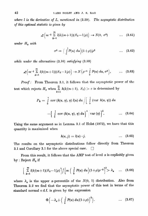
where I is the derivative of L, mentioned in (3.59). The asymptotic distribution
of this optimal statistic is given by
i m \ cQlm-t 2
l(kj(m+l))(Sk-ljp)) ->X(0, <r2) ... (3.61)
under H0 with
or* = I ?l\u) du)(l+p)jp2
... (3.62)
while under the alternatives (3.10) satisfying (3.59)
I m . , i .
Arnr* 2 l(kj(m+l))(Sk~ljp)) ->X(/>-1 J Z2(^) dw,-cra , ... (3.63) \ k=i / o /
Proof : From Theorem 3.1, it follows that the asymptotic power of the m
test which rejects HQ when 2 h(kj(m-j-l), Sk) > c is determined by ?=l
1 / r 1
Ph = j cov (?(^, 7/), ?/) l(u) du / J* (var h(u, t?)) du
f 1 ,2 -i*
- J J cov (A(w, ?/), 7/) dw > / var (r?) . ... (3.64)
Using the same argument as in Lemma 3.1 of Hoist (1972), we have that this
quantity is maximized when
h(u,j) =
l(u)-j. ... (3.65)
The results on the asymptotic distributions follow directly from Theorem
3.1 and Corollary 3.1 for the above special case.
From this result, it follows that the AMP test of level a is explicitly given
by : Reject HQ if
r rn - r , i i ni
j V_l{kj{m+\){Sk-ljp) j j \m ( J l*(u) duj(l+p)p^ ] > Aa ... (3.66)
where Aa is the upper a-percentile of the iV(0, 1) distribution. Also from
Theorem 3.2 we find that the asymptotic power of this test in terms of the
standard normal c.d.f. is given by the expression
*(-*?+( Sl2Wduj(l+p)f). ... (3.67)
TWO-SAMPLE NONPARAMETRIC STATISTICS 43
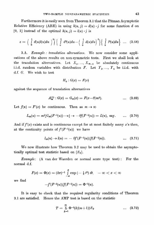
Furthermore it is easily seen from Theorem 3.1 that the Pitman Asymptotic Relative Efficiency (ARE) in using h(u, j)
= d(u) >j for some function d on
[0, 1] instead of the optimal h(u,j) = l(u) j is
e = / f d(u)l(u)du \2j { J d2(u)du-( } d(u)du\ 2}j J Z2(^)cfel ... (3.68)
3.A. Example : translation alternatives. We now consider some appli cations of the above results on non-symmetric tests. First we shall look at
the translation alternatives. Let Xv ..., Xm_1 be absolutely continuous
i.i.d. random variables with distribution F. Let Yl9 ..., Yn be i.i.d. with
d.f. G. We wish to test
#0 : G(x) = F(x)
against the sequence of translation alternatives
A&> : G(x) =
Gm(x) =
F(x-d\m?). ... (3.69)
Let f(x) =
Ff(x) be continuous. Then as m ?> oo
Lm(u) =
m\Gm(F-\u))-u\ -> -df(F~\u)) =
L(u), say. ... (3.70)
And iff'(x) exists and is continuous except for at most finitely many #'s then, at the continuity points of fr(F~\u)) we have
Uu) -> l(u) = - 6f\F-\u))lf{F-\v)). ... (3.71)
We now illustrate how Theorem 3.2 may be used to obtain the asympto
tically optimal test statistic based on {Sk}.
Example : (A van der Waerden or normal score type test) : For the
normal d.f.
F(x) =
<J>(x) =
(2n)~* J exp (- \t^)dt, - oo < x < oo
? ao
we find
-f'(F-\u))lf(F-\u)) = 4>-H?).
It is easy to check that the required regularity conditions of Theorem
3.1 are satisfied. Hence the AMP test is based on the statistic
m T= S (D-^m+l))?* ... (3.72)
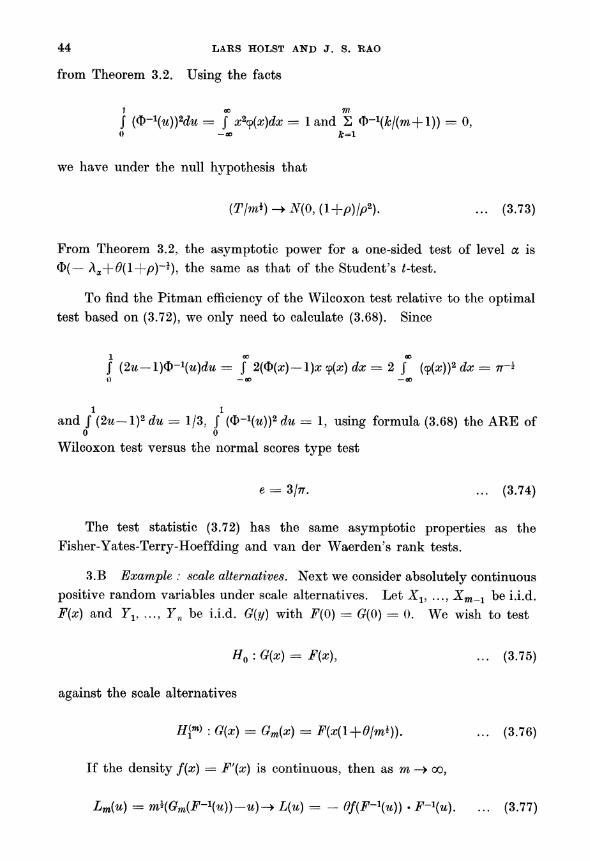
44 LARS HOLST AND J. S. RAO
from Theorem 3.2. Using the facts
1 ? m
J (O-1^))2^ = J x2y(x)dx = 1 and 2 O-^Jk/im+l))
= 0, 0 -ao fc=l
we have under the null hypothesis that
(T/w*) -> N(0, (l+p)?p2). ... (3.73)
From Theorem 3.2, the asymptotic power for a one-sided test of level a is
0( ?
Aa+0(1+/?)-*), the same as that of the Student's ?-test.
To find the Pitman efficiency of the Wilcoxon test relative to the optimal test based on (3.72), we only need to calculate (3.68). Since
.J (2u-l)Q)-1(u)du = f 2(?(x)-l)x y(x) dx = 2 f (<p(x))2 dx = 77-*
0 ? oo ? oo
1 1
and J (2u-~l)2du =
1/3, J (<S>-\u)Y du = 1, using formula (3.68) the ARE of o o
Wilcoxon test versus the normal scores type test
e = 3/tt. ... (3.74)
The test statistic (3.72) has the same asymptotic properties as the
Fisher-Yates-Terry-Hoeffding and van der Waerden's rank tests.
3.B Example : scale alternatives. Next we consider absolutely continuous
positive random variables under scale alternatives. Let Xv ..., Xm_x be i.i.d.
F(x) and Yv ..., Yn be i.i.d. G(y) with F(0) =
0(0) = 0. We wish to test
H0:G(x)= F(x), ... (3.75)
against the scale alternatives
H["> : G(x) =
Gm(x) =
F(x(l+6?m^)). ... (3.76)
If the density f(x) =
F'(x) is continuous, then as m ?> oo,
Lm(u) =
m^GUF-^uV-u)-* L(u) = -
df(F~\u)) . F~\u). ... (3.77)
TWO-SAMPLE NONPARAMETRTO STATISTICS 45
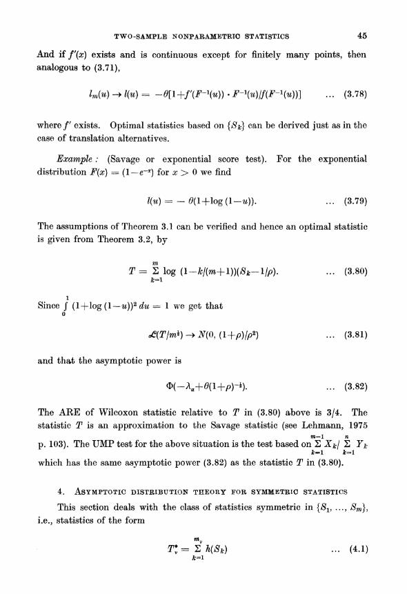
And if f'(x) exists and is continuous except for finitely many points, then
analogous to (3.71),
Uu) -> if*) = -d[l +f'(F-\u)) - F-\u)jf(F-\u))} ... (3.78)
where /' exists. Optimal statistics based on {Sk} can be derived just as in the
case of translation alternatives.
Example : (Savage or exponential score test). For the exponential distribution F(x)
= (1?e~x) for x > 0 we find
l(u) = -
#(l+log(l-*?)). ... (3.79)
The assumptions of Theorem 3.1 can be verified and hence an optimal statistic
is given from Theorem 3.2, by
m T= 2 log (l-kj(m+l))(Sk-ljp). ... (3.80)
fc=i
i
Since j (l+log(l?u))2du = 1 we get that
o
c?{Tjm*) -> N(0, (l+p)jp2) ... (3.81)
and that the asymptotic power is
?(-Aa+d(l+p)-i). ... (3.82)
The ARE of Wilcoxon statistic relative to T in (3.80) above is 3/4. The
statistic T is an approximation to the Savage statistic (see Lehmann, 1975 m?1 n
p. 103). The UMP test for the above situation is the test based on 2 Xkj 2 Yk k=*l fc=l
which has the same asymptotic power (3.82) as the statistic T in (3.80).
4. Asymptotic distribution theory for symmetric statistics
This section deals with the class of statistics symmetric in {Sv ..., Sm],
i.e., statistics of the form
T*= ?h(Sk) ... (4.1)
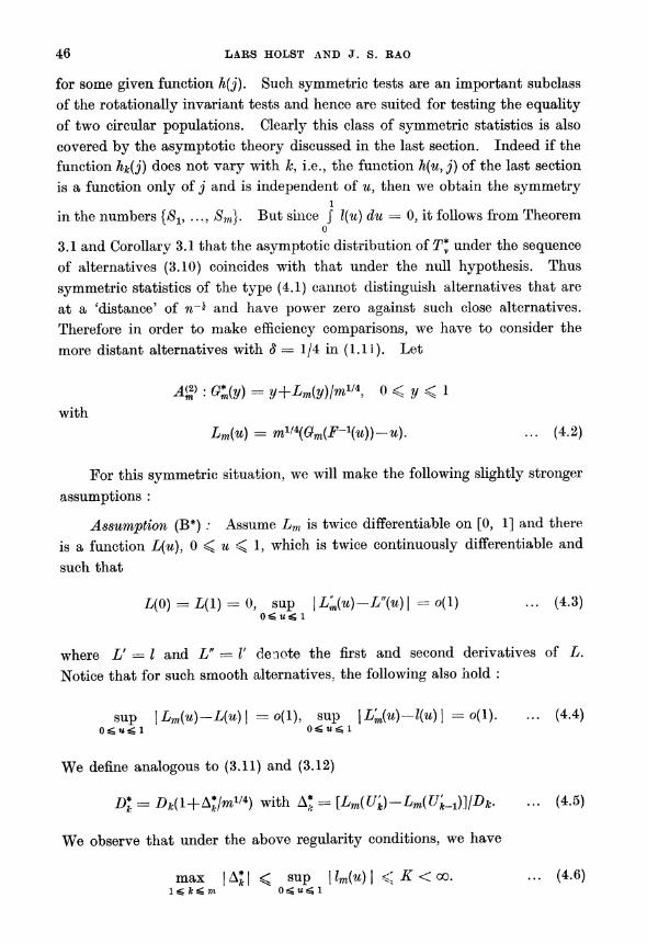
46 LARS HOLST AND J. S. RAO
for some given function h(j). Such symmetric tests are an important subclass
of the rotationally invariant tests and hence are suited for testing the equality
of two circular populations. Clearly this class of symmetric statistics is also
covered by the asymptotic theory discussed in the last section. Indeed if the
function hk(j) does not vary with k, i.e., the function h(u,j) of the last section
is a function only of j and is independent of u, then we obtain the symmetry i
in the numbers [Sl9 ..., Sm}. But since J l(u) du = 0, it follows from Theorem o
3.1 and Corollary 3.1 that the asymptotic distribution of?7* under the sequence
of alternatives (3.10) coincides with that under the null hypothesis. Thus
symmetric statistics of the type (4.1) cannot distinguish alternatives that are
at a 'distance' of n~* and have power zero against such close alternatives.
Therefore in order to make efficiency comparisons, we have to consider the
more distant alternatives with 8 = 1/4 in (1.11). Let
4? : G&y) = y+Lmiy)?mW, 0 < y < 1
with
Lm(u) =
mV\Gm{F-\u))-u). ... (4.2)
For this symmetric situation, we will make the following slightly stronger
assumptions :
Assumption (B*) : Assume Lm is twice differentiate on [0, 1] and there
is a function L(u), 0 < u < 1, which is twice continuously differentiable and
such that
?(0) =
?(1) - 0, sup \L?(u)--L\u)\
= o(l) ... (4.3)
where V = I and L" = V denote the first and second derivatives of L.
Notice that for such smooth alternatives, the following also hold :
sup \Lm(u)-L(u)\ =o(l), sup \L'm(u)-l{u)\ =
o(l). ... (4.4)
We define analogous to (3.11) and (3.12)
D? =
Dk(l+Aljmv*) with A*c =
[Lm(Uh)-Lm(Uk_x)]IDk. ... (4.5)
We observe that under the above regularity conditions, we have
max |AJ| < sup \lm(u)\ < K < oo. ... (4.6) 1^ k^m 0^ m^1

TWO-SAMPLE NONPARAMETRIC STATISTICS 47
The following theorem gives the asymptotic distribution of the symmetric statistics T* under the alternatives (4.2).
Theorem 4.1 : Suppose that there exist constants c? and c2 such that
\Mj)\ <c1(/2+l)/oraZZj. ... (4.7)
Let Lm(u) satisfy Assumption^*) and let
m
P;= 2 (h(Sk)-Eh(7i))?m^cr ... (4.8) fc=i
where a2 = var (h(7?))?[cov (h(r?), r?)]2?var (r?) ... (4.9)
and t? is the geometric random variable defined in (1.9). Then under the
alternatives (4.2)
<?(V*)->N(A, 1) as v -> oo ... (4.10)
where
A=[\ l2(u)du\ cov(h(7?), 7i(7}-l)-47ilp)p2l2(l+p)2(T. ... (4.11)
Proof : Following the method used in the proof of Theorem 3.1, it suffices
to show that
m~* [fly(nD*)~ju,v(nD)] ?>A in probability. We have
m-*[ju,v(nD*)-fiv(nD)]
m oo = m-* 2 2 hU^n^nDD-rr^nDfc)]
m oo = m-* S 2 h(j)n}(nDk)[( 1 + A*/??1'*)/ exp (
- raZ>*A?t/m1'4)
fc=l ?=o
_l_j_WjDA;A*/m1/*-{j(j-l)-2>2)&+(?I>i)2}A|/m* m oo
+w-?>4 2 2 h(j) TrunD?iJ-nDjk) A* fc=i y=o
?? 00
+WI-1 2 V m)n}{nDk){j(3-l)-23nDk+{nDk)*} ?%\2. ... (4.12)

48 LARS HOLST AND J. S. RA?
After some direct but tedious calculations, it may be verified that the
probability limits of the first two terms on the RHS of (4.12) are zero while
that of the third term is
( J l\u)du)
- (cov (%), v(v-l)-mP) -p2j2(l+p)2 )
under the assumptions, thus completing the proof.
Taking l(u) = 0, 0 < u < 1 in Theorem 4.1 or putting hk(j) =
h(j) -y- k
in Corollaries 3.1, 3.1', we get the following result on the asymptotic null
distribution for the symmetric statistics.
Corollary 4.1 : Let V*v be as defined in (4.8). Then under the null hypothesis
(1.1) F* has asymptotically a N(0, 1) distribution if the function h( ) satisfies condition (4.7).
As in Theorem 3.2, we now consider a result on the optimal choice of the
function h( ) for the symmetric case.
Theorem 4.2 : For the sequence of alternatives given by (4.2), satisfying the conditions of Theorem 4.1, the asymptotically most powerful (AMP) test is of the form : Reject H0 when
m 2 Sk(8k-l)>c. ... (4.13) k=l
Proof : From Theorem 4.1, it follows that the asymptotic power of a
test of the form (4.1) is a maximum when the quantity A given in (4.11) is
maximized. Observe that
cov (r?, r?(7j?l)??7ijp) = 0 ... (4.14)
and
var (h(r?)) ? cov2 (h(y), 7j)j var (r?)
? var (h(7j)??ri) ... (4.15)
where ? is the usual linear regression coefficient
? = cov (h(r?), 7/)/var (r?). ... (4.16)
Therefore we can rewrite
2p-2(\+p)2Aj J l2(u)du = cov (h(ri)-?ri, r){<r?- l)-4?///>)/[var (%)-^)]* o = cor (%)-/??/, 7i(t)-1)-4:7iIp) [var M?/-l)-4^//>)]*
< [var (ti(V-l)-4?/p)]* = 2p~*(l+p) ... (4.17)
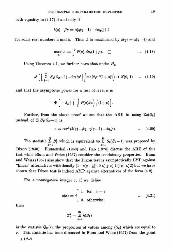
TWO-SAMPLE NONPARAM?TRIC STATISTICS 49
with equality in (4.17) if and only if
for some real numbers a and b. Thus A is maximized by h(7?) =
r?(ri?l) and
maxi = J* Z2(w) du?(l+p). Q (4-18)
? 0
Using Theorem 4.1, we further have that under H0,
off ( [ 2^ ?*(?*-l)-2m//| im^pp-^l+p)])^^,
1) ... (4.19)
and that the asymptotic power for a test of level a is
?[-k+( }nu)du)j(i+p)]. Further, from the above proof we see that the ARE in using Hh(Sk)
instead of 2 Sk(Sk? 1) is
e = cor2(h(7?)? ?y} t?(t?? 1)??7\\p).
... (4.20)
m m
The statistic 2 SI which is equivalent to 2 Sk(Sk? 1) was proposed by *=1 k**l
Dixon (1940). Blumenthal (1963) and Rao (1976) discuss the ARE of this test while Blum and Weiss (1957) consider the consistency properties. Blum
and Weiss (1957) also show that the Dixon test is asymptotically LMP against "linear" alternatives with density {l+c(y?|)}, 0<y<l(|c|<2) but we have
shown that Dixon test is indeed AMP against alternatives of the form (4.2).
For a nonnegative integer r, if we define
f 1 for x = r
otherwise, then
h(x)=< ... (4.21)
I 0
m T*v
= 2 h(Sk) fc=i
is the statistic Qw(r), the proporiton of values among {Sk} which are equal to
r. This statistic has been discussed in Blum and Weiss (1957) from the point
A12-7
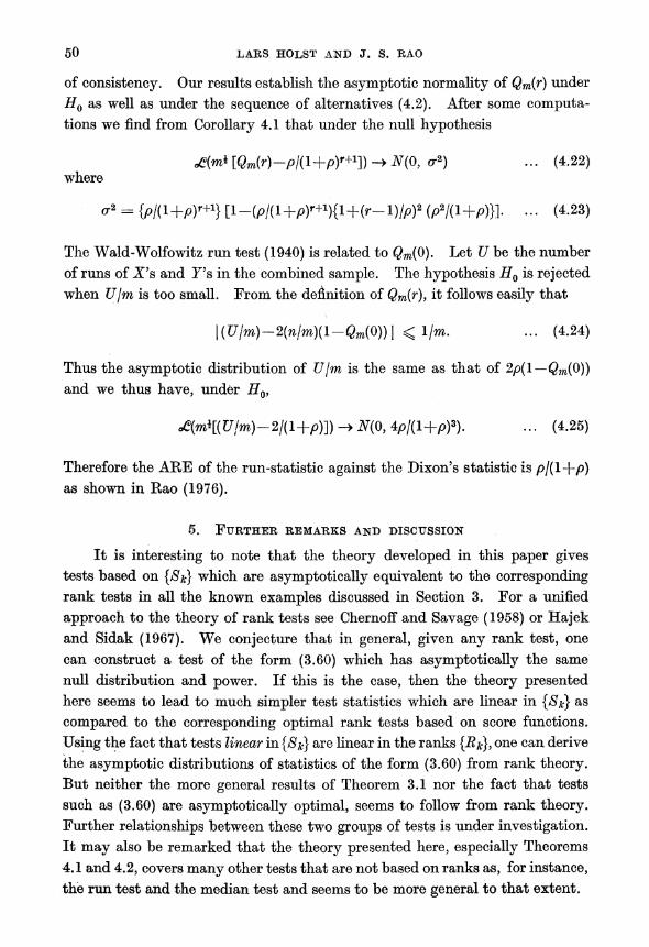
50 LARS HOLST AND J. S. RAO
of consistency. Our results establish the asymptotic normality of Qm{r) under
H0 as well as under the sequence of alternatives (4.2). After some computa
tions we find from Corollary 4.1 that under the null hypothesis
A nQm(r)-pl(I+p)r+1]) ~> N(0, or2) ... (4.22) where
^2 = W(l+P)r+1}[l-(W(l+P)r+1){l+(^- -. (4-23)
The Wald-Wolfowitz run test (1940) is related to Qm(0). Let U be the number
of runs of X's and 7's in the combined sample. The hypothesis H0 is rejected when Ujm is too small. From the definition of Qm(r), it follows easily that
\(Ujm)-2(njm)(l-Qm(0))\ < 1/m. ... (4.24)
Thus the asymptotic distribution of Ujm is the same as that of 2p(l?Qm(0)) and we thus have, under H0,
t?(mK(Ujm)-2j(l+p)]) -> N(0, 4p/(l+p)3). ... (4.25)
Therefore the ARE of the run-statistic against the Dixon's statistic is pj(l+p) as shown in Rao (1976).
5. Further remarks and discussion
It is interesting to note that the theory developed in this paper gives tests based on {Sk} which are asymptotically equivalent to the corresponding rank tests in all the known examples discussed in Section 3. For a unified
approach to the theory of rank tests see Chernoff and Savage (1958) or Hajek and Sidak (1967). We conjecture that in general, given any rank test, one
can construct a test of the form (3.60) which has asymptotically the same
null distribution and power. If this is the case, then the theory presented here seems to lead to much simpler test statistics which are linear in {Sk} as
compared to the corresponding optimal rank tests based on score functions.
Using the fact that tests linear in {Sk} are linear in the ranks {Rk},
one can derive
the asymptotic distributions of statistics of the form (3.60) from rank theory. But neither the more general results of Theorem 3.1 nor the fact that tests
such as (3.60) are asymptotically optimal, seems to follow from rank theory. Further relationships between these two groups of tests is under investigation. It may also be remarked that the theory presented here, especially Theorems
4.1 and 4.2, covers many other tests that are not based on ranks as, for instance,
the run test and the median test and seems to be more general to that extent.
TWO-SAMPLE NONPARAMETRIC STATISTICS 51
The theorems presented here can also be applied to study similar test
statistics when the samples are censored. For instance, suppose that the
samples are censored at the right by X[{m_1)qj, the [(m?l)q]-th order statistic
in the X-sample. Under the same assumptions as in Theorem 3.2, we obtain
in the same way that optimal test statistic is given by
[(m-i)ff]
T= 2 l(k\(m+l))(Sk-l\p). ... (5.1) ?=i
Under H0,
?(T\m?) -? N(0, f / l2(u)du- (f l(u)du))*}(p+l)/p2)
and the asymptotic power is
0(-Aa+ ( J
l2(u)duj{ [/ l2(u)du- (/ l(u)du^\ (l+p)}V2)).
... (5.2)
For results on censoring in rank theory see, for instance, Rao, Savage and
Sobel (1960) or Johnson and Mehrotra (1972).
Acknowledgement. The authors wish to thank the referee whose comments
led to many improvements in the presentation of this paper.
References
Blum, J. R. and Weiss, L. (1957) : Consistency of certain two-sample tests. Ann. Math. Statist.,
28, 242-246.
Blumenthal, S. (1963) : The asymptotic normality of two test statistics associated with the
two-sample problem. Ann. Math. Statist., 34, 1513-1523.
Chernoff, H. and Savage, I. R. (1958) : Asymptotic normality and efficiency of certain non
parametric statistics. Ann. Math. Statist., 29, 972-994.
Darling, D. A. (1953) : On a class of problems related to the random division of an interval.
Ann. Math. Statist., 24, 239-253.
Dixon, W. J. (1940) : A criterion for testing the hypothesis that two samples are from the same
population. Ann. Math. Statist., 11, 199-204.
Godambe, V. P. (1961) : On the two-sample problem : A heuristic method for constructing
tests. Ann. Math. Statist,, 32, 1091-1107. / v /
Hajek, J. and Sidak, Z. (1967) : Theory of Rank Tests, Academic Press, New York.
Holst, L. (1972) : Asymptotic normality and efficiency for certain goodness of fit tests. Bio
metrika, 59, 137-145.
-(1979) : Two conditional limit theorems with applications, Ann. Statist., 7, 551-559.
Johnson, R. A. and Mehrotra, K. G. (1972) : Locally most powerful rank tests for the two
sample problem with censored data, Ann. Math. Statist., 43, 823-831.
52 LARS HOLST AND J. S. RAO
Le Cam, L. (1958) : Un th?orems sur la division (Tun intervalle par des points pris au hasard.
Pub. Inst. Statist. Univ. Paris, 7, 7-16.
Lehmann, E. L. (1975): Nonparametric Statistical Methods Based on Ranks, Holden-Dey, Inc.,
San Francisco.
Pyke, R. (1965) : Spacings. Jour. Roy. Statist. Soc, Ser. B, 27, 395-449.
Rao, J. S. (1976) : Some tests based on arc lengths for the circle. Sankhy?, Ser. B, 38, 329-338.
Rao, J. S. and Holst, L. (1980) : Some results on the asymptotic spacings theory. Submitted
for publication.
Rao, J. S. and Sethtjraman, J. (1975) : Weak convergence of empirical distribution functions
of random variables subject to perturbations and scale factors. Ann. Statist., 3, 299-313.
Rao, U. V. R., Savage, I. R. and Sobel, M. (1960) : Contributions to the theory of rank order
statistics : The two sample censored case. Ann. Math. Statist., 31, 415-426.
Wald, A. and Wolfowitz, J. (1940) : On a test whether two samples are from the same popula
tion. Ann. Math. Statist., 11, 147-162.
Paper received : January, 1979.
Revised : August, 1979.