Embed Size (px)
Citation preview

FI+WA/i^'^h-i l.
f Ju €


JOINT HIGHWAY RESEARCH PROJECT
FHWA/IN/JHRP-84 /20
INDIANA HIGHWAY COST ALLOCATION
STUDY: FINAL REPORT
K. C. Sinha
T. F. FwaE. A. SharafA. B. Tee
H. L. Michael

TECHNICAL REPORT STANDARD TITLE PACE
1 . Report No.
FHWA/IN/JHRP-84/20
2, Government Accession No.
«. Title and SublilU
INDIANA HIGHWAY COST-ALLOCATION STUDY: FINAL
REPORT
Kumares C. Sinha, Tien-Fang Fwa, Essam A. Sharaf,
Ah-Beng Tee and Harold L. Michael
9. Performing Orgoniiotion Nome ond Address
Joint Highway Research Project
Civil Engineering Building
Purdue UniversityWest Lafayette, Indiana 47907
12. Sponsoring Agency Nome ond Addres-
Indiana Department of Highways
State Office Building100 North Senate AvenueIndianapolis, Indiana 46204
3. Recipient's Co'olog No.
S. Report Do-. ,),. ,,,!„.. ,|f
|(|H/|
L^vJ^uuL^iri ii. i'Jii.
6. Perl orming Urgo ii loll on Code
8. Performing Orgoniiotion Peporl No
JHRP-84-20
10. Wo,W Unit No.
11. Controct or Grant No.
HPR-Part I
13. Type of Report ond Period Covered
Final Report
u. sponi on ng *gAgenc y Code
15. Supplementory Note!
Conducted in cooperation with the U.S. Department of Transportation, Federal
Highway Administration.
16. Abstract
This final report presents the findings of the highway cost-allocation
study in Indiana. The cost responsibilities and revenue contributions of
various vehicle classes were determined for FY 1983 and the biennial period
of 1985-86. The findings indicate that passenger cars and single-unit trucks
are overpaying their cost responsibility, while buses and heavy combination
trucks are underpaying. The report also includes a summary of the procedures
used. A thickness incremental approach was used to allocate new highway
construction cost and an integrated approach was followed to allocate highway
rehabilitation and routine maintenance costs. The structure-related costs
were allocated by an incremental analysis. An explicit consideration was
given to the effects of age, weather, salt and other chemicals on highways.
17. Key Words
highway cost allocation; revenue
attribution; cost responsibility.
19. Security Clossif. (of this report)
Unclassified
IB. Distribution Stctemtnt
No restrictions. This document is
available to the public through the
National Technical Information Service,
Springfield, VA 22161
20. Security Close!!, (of this pose 1
Unclassified
21. No. of P o;es
259
22. P'C
Form DOT F 1700.7 (e-6»>

INDIANA HIGHWAY COST- ALLOCAT I ON STUDYFINAL REPORT
To: U.L. Michael, DirectorJoint Highway Research Project
From: K.C. Sinha, Research EngineerJoint Highway Research Project
October 31 , 1984Revised March, 1983
Project :
File:C-36-54PP3-3-42
Attached is the Final Report on the HPR Part I Study titled,"Indiana Highway Cost-Allocation Study." This report presents thefindings of the cost-allocation study for Indiana and it has beenprepared under the direction of Professor K. C. Sinha.
The methodology conforms to the mandate of the H.E.A. 1006of the 103rd General Assembly. The findings indicate that thepassenger cars and single-unit trucks are overpaying their costresponsibility, while the buses and heavy combination trucks areunderpaying their cost responsibility.
This report is forwarded for review, comment and acceptanceby the IDOH and FHWA as fulfillment of the objectives of thestudy.
Respectfully submitted,
K.C' SinhaResearch Engineer
KCS/rrp
cc A.G. Alt s chae f f 1 W.H. Goe tz C.F . Sch o le r
J.M. Bell G.K. Hallock R.M. Shant eauW.F. Chen J .F . McLaugh 1 i n K.C . SinhaW.L. Dolch R.D. Miles C.A. Ve na b leR.L. Eskew P .L . Owens L.E . WoodJ .D. Fri eke r B.K. Partridge S .R. YoderJ .R. Skinne r G.T. Sat t e r ly

INDIANA HIGHWAY COST-ALLOCATION STUDY:FINAL REPORT
by
Kuma res C . S
[
nha
Professor of Transportation Engineering
Tien-Fang Fwa
Graduate Research Assistant
Ess am A. Sharaf
Post-Doctoral Research Fellow
Ah-Beng Tee
Graduate Research Assistant
Harold L. Michael
Professor of Civil Engineering
Joint Highway Research Project
Project No: C-36-54PP
File No: 3-3-42
Prepared as Part of an Investigation
Conducted by
Joint Highway Research ProjectEngineering Experiment Station
Purdue University
in cooperation with the
Indiana Department of Highways
and the
U.S. Department of TransportationFederal Highway Administration
The contents of this report reflect the views of the. authorswho are responsible for the facts and the accuracy of the datapresented herein. The contents do not necessarily reflect theofficial views or policies of the Federal Highway Administra-tion. This report does not constitute a standard, specifica-tion, or regulation.
Purdue UniversityWest Lafayette, Indiana
October 31 , 1984
Revised March, 1985

Digitized by the Internet Archive
in 2011 with funding from
LYRASIS members and Sloan Foundation; Indiana Department of Transportation
http://www.archive.org/details/indianahighwaycoOOsinh

ACKNOWLEDGMENTS
The preparation of the report was financially supported by the Federal
Highway Administration and Indiana Department of Highways. The guidance and
counsel of Mr. Gene K. Hallock, Director of the Indiana Department of Highways
is greatly appreciated. The assistance of Messrs. Charles Basner and Gary
Dalporto of the Federal Highway Administration and Messrs. Daniel Novreske,
Deputy Director of Administration and Larry Scott and Don Houterloot of the
Planning Division of the Indiana Department of Highways has made the study
possible. In addition, many individuals at the Indiana Department of Highways
have provided data and necessary information, including Messrs. Richard A.
Payne of the Accounting Division, Stanley R. Yoder and Steven J. Hull of the
Design Division, David L. Tolbert of the Computer Services Division, William
J. Rittman of the Construction Division, William T. May of the Contracts and
Legal Division, Robert E. Woods of the Local Assistance Division, Kenneth M.
Mellinger and R. Clay Whitmire of the Maintenance Division, Barry Partridge
and Keith J. Kercher of the Research and Training Division, and Clinton A.
Venable of the Traffic Division. Many students and faculty members at Purdue
University contributed to the study, including Messrs. Mark Henderson, Paul
Satterly, John D. N. Riverson, Greg Turk, Mitsuru Saito and Khaled Ksaibati,
and Profs. Virgil L. Anderson, Robert H. Lee, Robert M. Shanteau and Edward C.
Ting. The assistance of Mr. Fred Ross of the Wisconsin Department of Transpor-
tation in the early phase of the study is acknowledged. Acknowledgment is
also extended to Mrs. Rita Pritchett and Mrs. Julia Jordan who typed the
report.
TABLE OF CONTENTS
Page
LIST OF TABLES v
LIST OF FIGURES xi
EXECUTIVE SUMMARY xi i i
CHAPTER 1. INTRODUCTION 1
Purpose of the StudyHighway ClassificationVehicle Classification 4
Definition of CostsTime Frame of Study 9
Allocated Costs 9
Attributed Revenues 14
CHAPTER 2. COST ALLOCATION METHODOLOGY 18
Guiding Principles 18Overview of the Study Approach 19Summary of Cost-Allocation and Revenue-Attribution
Procedures 22
CHAPTER 3. RESULTS OF COST-ALLOCATION AND REVENUE-ATTRIBUTIONANALYSIS 27
Cost-Responsibility Factors for Highway and StructureExpenditure Items 27
Cost-Responsibility Factors for Major ExpenditureAreas 29
Overall Statewide Vehicle Class Cost-Responsibilities 35
Proportions of Attributable and Non-AttributableCosts 38
Revenue Contribution by Vehicle Class 4 2
Comparison of Cost Responsibility with RevenueContribution 42
Base Period (1983) Findings 42Biennial Budget Period (1985-86) Findings .... 44
Comparison of Indiana's Findings to Findings inOther Studies 45
CHAPTER 4. CONCLUSIONS 47
APPENDIX A. DATA BASE 50
Traffic Data 50
li

Cost Data
State Highway System 5 1
Local Roads
Revenue Data
APPENDIX B. PROCEDURE FOR TRAFFIC DATA COLLECTION
Vehicle CountField Data Collection ProceduresData Reduction and AnalysisEstimation of Vehicle-Miles of Travel 60VMT Correspondence Matrices for Registered and
Operating Weight Groups 67
APPENDIX C. HIGHWAY CONSTRUCTION COST ALLOCATION 87
GeneralRight-of-Way Costs 87
Grading and Earthwork Costs 91
Drainage and Erosion Control Costs 94
New Pavement Costs 97
Shoulder Costs 105
Re construction Costs 107
Miscellaneous Items 108
APPENDIX D. HIGHWAY REHABILITATION COST ALLOCATION 109
General 109
Previous Studies 109
Allocation Procedure for Pavement RehabilitationCosts Ill
APPENDIX E. STRUCTURAL CONSTRUCTION, REPLACEMENT ANDREHABILITATION COST ALLOCATION 117
General 117
Adopted Incremental Method 118Design Loadings 118Correlation Between AASHT0 and Actual Trucks 119Selection of Bridge Samples 121
Variation of Structure Width with Live Loadings 126Distribution Between Highway and Waterway Crossings .. 128Allocation Factors 128
Superstructure Cost Factors 131
Substructure Cost Factors 133
Excavation and Backfill Factors 148
Drainage Pipe Factors 148
Railing Factors 148
Miscellaneous Items 15C
in

Allocation of Cost Responsibilities 150New Bridge Construction 15 2
Bridge Re placement 152Bridge Rehabilitation 154
Culverts 154
Sign Bridges 157
APPENDIX F. MAINTENANCE COST ALLOCATION 159
General 159Previous Studies 159Allocation Methodology 160Data Base for Analysis 162Procedure for Allocating Pavement Routine Maintenance
Costs 162
APPENDIX G. REVENUE ATTRIBUTION 165
State Highway Revenues 165Federal Revenues 167Attribution of Revenue 167
State Fuel Taxes 168State Registration Fees 169Other Taxes and Fees 170Federal Taxes 170
APPENDIX H. DETERMINATION OF COST-RESPONSIBILITY FACTORSOF LOAD-RELATED AND NON-LOAD-RELATED FACTORS INPAVEMENT REHABILITATION AND MAINTENANCE COSTALLOCATION 172
APPENDIX I. TABLES OF COST-RESPONSIBILITY FACTORS USED FORCOST-ALLOCATION COMPUTATION 183
APPENDIX J. PROBLEMS OF USING CENTS PER VEHICLE-MILES OFTRAVEL AS AN INDEX FOR EXPRESSING CO ST- ALLOCATIONRESULTS 23A
REFERENCES 239
- IV

LIST OF TABLES
Tab le
1
2
3
4
5
9
10
1 1
B. 1
B.2
B.3
B.4
B. 5
B . 6
B.7
B. 9
Page
Adopted Vehicle Classification 6
Vehicle Class Weight Group Classification 7
Expenditure Items by Expenditure Area 10
Highway User Revenues 17
Overall Statewide Cost-Responsibility for Year1983 36
Overall Statewide Cost-Responsibility for Year1985-86 37
Cost Allocation Criteria for Expenditure Items .... 39
Revenue Contribution by Vehicle Class (1983) 40
Revenue Contribution by Vehicle Class (1985-86) ... 41
Cost-Allocation and Revenue Attribution Summary ... 43
Comparison of Findings of the Indiana Study toFindings of Other Studies 46
Number of Traffic Count Sites 56
Volume Count Station Locations 57
Percent VMT of Vehicle Classes on Rural Interstate(1983) 61
Percent VMT of Vehicle Classes on Urban Interstate(1983) -
:
Percent VMT of Vehicle Classes on State Primarv(1983) ; 63
Percent VMT of Vehicle Classes on State Secondary(1983) 64
Percent VMT of Vehicle Classes on County Roads(19 8 3) 65
Percent VMT of Vehicle Classes on City Streets(1983)
Percent VMT of Vehicle Classes on Rural Interstate

(1985-86) 69
B.10 Percent VMT of Vehicle Classes on Urban Interstate(1985-86)
B.ll Percent VMT of Vehicle Classes on State PrimaryRoutes (1985-86)
B.12 Percent VMT of Vehicle Classes on State SecondaryRoutes (1985-86)
B.13 Percent VMT of Vehicle Classes on County Roads(1985-86)
B.14 Percent VMT of Vehicle Classes on City Streets(1985-86) 74
B.15 VMT Values by Highway Functional Class
B.16 Indiana Bureau of Motor Vehicles RegisteredVehicle Classification
B.17 Vehicle Registration Weight-Operating WeightCorrespondence Matrix for Single-Unit TrucksClass 3
B.18 Vehicle Registration Weight-Operating WeightCorrespondence Matrix for Single-Unit TrucksClass 6
B.19 Vehicle Registration Weigh t -Ope rat ing WeightCorrespondence Matrix for Combination TrucksClass 7 79
B.20 Vehicle Registration Weight-Operating WeightCorrespondence Matrix for Single-Unit TrucksClass 9
B.21 Vehicle Registration Weigh t -Ope rat ing WeightCorrespondence Matrix for Combination TrucksClass 10 81
B.22 Vehicle Registration Weight-Operating WeightCorrespondence Matrix for Combination TrucksClass 11 82
B.23 Vehicle Registration We igh t -Ope ra t i ng WeightCorrespondence Matrix for Combination TrucksClass 12
B.24 Vehicle Registration We i gh
t
-Op e ra t i ng WeightCorrespondence Matrix for Combination TrucksClass 13 85
- vi -

B.25 Vehicle Registration We igh t -Ope ra t i ng WeightCorrespondence Matrix for Combination TrucksClass 14 8 6
C.l Right-of-Way Width Requirements 89
C.2 Traveled-Way Width Requirements 93
E.l Study Vehicle Classification and EquivalentAASHTO Designation 122
E.2 Vehicular Classification and Responsibility Summaryfor Bridge Superstructure 123
E.3 Characteristics of Typical Bridges Constructedin the Base Period 127
E.4 Bridge Width Under Different Loadings 129
E.5 Distribution Between Highway and WaterwayCrossings 130
E.6 Bridge Superstructure Unit Costs 134
E.7 Bridge Deck Area 135
E.8 Superstructure Cost Factors for Interstate RuralBridges 136
E.9 Superstructure Cost Factors for Interstate UrbanBridges 137
E.10 Superstructure Cost Factors for State PrimaryHighway Bridges 138
E.ll Superstructure Cost Factors for Secondary HighwayBridges 139
E.12 Superstructure Cost Factors for Local RoadBridges 140
E.13 Piling Cost Factors 147
E.14 Piers and Abutment Cost Factors 149
E.15 Railing Cost Factors 151
E.16 Percent Distribution of New Bridge ConstructionCost by Cost Item and by Highway Class 153
E.17 Percent Distribution of Bridge Replacement Cost byCost Item and by Highway Class 155

E.18 Percent Distribution of Bridge Rehabilitation Costby Cost Item and by Highway Class
F.l Pavement Routine Maintenance Activities 163
H.l Relationship Between Present Serviceability Index(PSI) and Roughness Number (RN) 176
H.2 Proportional Responsibilities of Load-Related andNon-Load-Related Factors in Indiana PavementRehabilitation and Maintenance Cost Allocation .... 181
1.1 Pavement Construction Cost-ResponsibilityFactors 184
1.2 Shoulder Construction Cost-ResponsibilityFactors •
1.3 Right-of-way Construction Cost-ResponsibilityFactors 186
1.4 Drainage & Erosion Control Cost-ResponsibilityFactors 187
1.5 Grading & Earthwork Cost-ResponsibilityFactors 188
1.6 Common Costs Cos t-Res ponsbi 1 i t y Factors 189
1.7 Truck-Only Common Costs Cost-ResponsibilityFactors 190
1.8 Pavement Construction Cost-Responsibility of
Vehicle Classes on Rural Interstate (1983) 191
1.9 Pavement Rehabilitation Cost-ResponsibilityFactors for Rural Interstate 192
1. 10 Pavement Rehabilitation Cost-ResponsibilityFactors for Urban Interstate 193
1. 11 Pavement Rehabilitation Cost-ResponsibilityFactors for State Routes Primary 194
1.12 Pavement Rehabilitation Cost-ResponsibilityFactors for State Routes Secondary 195
1.13 Pavement Rehabilitation Cost-ResponsibilityFactors for County Roads 196
1.14 Pavement Rehabilitation Cos t -Res pons i bi 1 i tyFactors for City Streets 197
vm

1.15
I. 16
1.17
I. 18
I. 19
1.20
1.21
1.22
1.23
1.24
1.25
1.26
1.27
1.28
1.29
1.30
1.3 1
1.32
1.33
1.34
I. 35
Pavement Maintenance Cost-ResponsibilityFactors for Rural Interstate 198
Pavement Maintenance Cost-ResponsibilityFactors for Urban Interstate 199
Pavement Maintenance Cost-ResponsibilityFactors for State Routes Primary 200
Pavement Maintenance Cost-ResponsibilityFactors for State Routes Secondary 201
Pavement Maintenance Cost-ResponsibilityFactors for County Roads 202
Pavement Maintenance Cost-ResponsibilityFactors for City Streets 203
Bridge Superstructure Cost-ResponsibilityFactors 204
Bridge Pier Cost-Responsibility Factors 205
Bridge Excavation Backfill Cost-ResponsibilityFactors 206
Bridge Drainage Cost-Responsibility Factors 207
Bridge Pile Cost-Responsibility Factors 208
Bridge Railing Cost-Responsibility Factors 209
Cost-Responsibility for State Highways (1983) 210
Cost-Responsibility for County Roads (1983) 211
Cost-Responsibility for City Streets (1983) 212
Cost-Responsibility for Bridges on StateHighways (1983) 213
Cost-Responsibility for Bridges on CountyRoads (1983) 214
Cost-Responsibility for Bridges on City Streets(1983) 215
Cost-Responsibility for Sign Bridges (1983) 216
Cost-Responsibility for Police Enforcement(1983) 217
Weigh Station Inspection Cost-Responsibility for
- ix -
Trucks (1983) 218
1.36 Cost-Responsibility for State Highways(1985-86) 219
1.37 Cost-Responsibility for County Roads (1985-86) .... 220
1.38 Cost-Responsibility for City Streets (1985-86) .... 22 1
1.39 Cost-Responsibility for Bridges on State Highways(1985-86) 222
1.40 Cost-Responsibility for Bridges on County Roads(1985-86) 223
1.41 Cost-Responsibility for Bridges on City Roads(1985-86) 12U
1.42 Cost-Responsibility for Sign Bridges (1985-86) .... 225
1.43 Cost-Responsibility for Police Enforcement(1985-86) 226
1.44 Weigh Station Inspection Cost-Responsibility forTrucks (1985-86) 227
1.45 Overall Cost-Responsibility for State HighwaySystem (1983) 228
1.46 Overall Cost-Responsibility for County Road System(1983) 229
1.47 Overall Cost-Responsibility for City Street System(1983) 230
1.48 Overall Cost-Responsibility for State HighwaySystem (1985-86) 231
1.49 Overall Cost-Responsibility for County Road System(1985-86) 232
1.50 Overall Cost-Responsibility for City Street System(1985-86) 233
J.l Cos t-Al locaion Analysis of Example Problem 234
J.2 Cost-Allocation of Example Problem Expressed inCents/VMT '. 238

LIST OF FIGURES
Figure Page
1 Expenditure Distribution for Fiscal Year 1983 12
2 Expenditure Distribution for Budget Year 1985-86 .. 13
3 Cost-Allocation Study Flow Chart 23
4 Computation of Overall Statewide Vehicle ClassCost-Responsibilities 30
5 Computation of Statewide Vehicle Class Cost-Responsibilities for State Highways 31
6 Computation of Statewide Cost-Responsibilitiesfor County Roads and City Streets 32
7 Derivation of Statewide Cost-Responsibilities forState Highway Bridges 33
8 Derivation of Statewide Cost-Responsibilities forBridges on County Roads and City Streets 34
D «l Schematic Diagram Showing Pavement PerformanceConsidered in Highway Rehabilitation CostAllocation 114
E.l Modified AASHTO Live Loading Configurations forBridge Incremental Designs 120
E.2 HS and H Trucks Correlation 124
E.3 Flow Chart Illustrating the Data Generation forthe Correlation Process 123
E.4 Percent of Total Superstructure Cost vs. AASHTOHS Loading for Interstate Urban Bridges 141
E.5 Percent of Total Superstructure Cost vs. AASHTOHS Loading for Interstate Rural Bridges 142
E.6 Percent of Total Superstructure Cost vs. AASHTOHS Loading for State Primary Bridges 143
E « 7 Percent of Total Superstructure Cost vs. AASHTOHS Loading for State Secondary Bridges 144
E « 8 Percent of Total Superstructure Cost vs. AASHTOHS Loading for Bridges on Local Roads 145
- xx -

G.l Organization of the Motor Vehicle Highway Account(MVHA) 166
H.l Total Pavement Damage as Defined by Zero-Maintenance Pavement Performance Curve 173
H.2 Schematic Diagram Showing Pavement PerformanceCurves with their Associated RoutineExpenditures 17 6
H.3 Schematic Diagram Showing Load-Related and Non-Load-Related Effects Responsible for PavementDamage 178
H.4 Northern and Southern Regions for Pavement Cost-Allocation 182
xii -

EXECUTIVE SUMMARY
Thi6 study was mandated by the House Enrolled Act 1006 of the 103rd Indi-
ana General Assembly and it was conducted by the Joint Highway Research Pro-
ject of Purdue University in cooperation with the Indiana Department of High-
ways.
The study documented the full cost of building and maintaining the
state's highway system including that portion of the Federal Interstate system
within Indiana. An equitable methodology based on an incremental approach was
developed for allocating such costs to all the users of the system. An expli-
cit consideration was given to the effects of age, weather, salt and other
chemicals on highways.
The study findings indicated a significant imbalance between cost respon-
sibility of and revenue payment by different vehicle classes. In FY 1983
passenger cars including panels and pickups as well as single-unit trucks
overpaid their cost responsibility, while heavy combination trucks and buses
underpaid their cost responsibility. The same pattern is expected in the
biennial period of 1985-86. However, the underpayment by heavy trucks would
be more pronounced in 1985-86. During this biennial period, passenger cars as
a group would be overpaying about 25% of their cost responsibility while
single-unit trucks as a group would be overpaying about 24% of their cost
responsibility. At the same time buses would pay about 2% less than their
cost responsibility and combination trucks as a group would pay about 46% less
than their cost responsibility.
xm -

Although the passenger cars as a group would overpay, there Is a signifi-
cant Inequity within this group. This inequity primarily involves underpay-
ment by small cars and overpayment by large cars. In 1985-86, small cars
would underpay about 24%, while large cars would overpay about 38"/ of their
cost responsibility. Also, among single-unit trucks, 2-axle and A-ax le trucks
would overpay by 45% and 3% respectively, while 3-axle trucks would underpay
by 18%. At the same time, almost all vehicle classes in heavy combination
group would underpay by about 50% except vehicle class 13 (other 5-axle) which
would overpay by about 20%.
In the two-year period of 1985-86 the passenger cars as a group would
overpay $197,960,000 and single-unit trucks as a group would overpay
$31,283,000. On the other hand, combination trucks would underpay
$229,130,000 and buses would underpay only $113,000. The subsidization of
heavy vehicles by passenger cars and single-unit trucks would thus continue if
the tax structure remains the same.
- XIV -

CHAI'TKR ONh
INTRODUCTION
The Indiana highway system consists of 11 ,294 miles of State Roads,
66,564 miles of County Roads and 13,818 miles of City Streets. The Federal-
Aid portion of the Indiana highway system is comprised of 1144 miles of Inter-
states, 5064 miles of Primary, 8980 miles of Secondary and 4828 miles of
Federal-Aid Urban highways. For all governmental units combined, annual
expenditures for highway purposes in Indiana are about 3/4 billion dollars.
As a part of the House Enrolled Act 1006, the 103rd Indiana General
Assembly required the Indiana Department of Highways (IDOH) "to undertake a
highway cost-allocation study to (a) document the full cost of building and
maintaining the state's highway system, including that portion of the Federal
Interstate system within Indiana; and (b) develop an equitable methodology for
allocating such costs to all the users of the system".
This study, entitled Indiana Highway Cost-Allocation Study, was initiated
by the Advisory Board of the Joint Highway Project of Purdue University in
cooperation with the IDOH on May 4, 1983. It was carried out in two phases.
The major tasks undertaken in Phase I are literature review, study design,
data collection and data analysis. Those included in Phase II are development
of the methodological framework, preparation of an interim report, determina-
tion of travel functions and current cost responsibility, sensitivity
analysis, future cost responsibility and preparation of a final report.
An interim report was issued during Phase II of this study. It examined
the methodology and procedures adopted by previous studies of other states to
determine cost responsibilities of various highway user groups. A procedure
for use in Indiana was discussed in the report [39]. This final report
1 -
presents the results, findings and conclusions of the entire study. A summ-iry
description of the cost-allocation procedures adopted is included in the
Appendices to this report.
Purpose o_f_ the Study
The main objective of this study was to fulfill the requirement of the
legislative directive mentioned earlier by determining the responsibility of
individual vehicle classes in occasioning highway costs. The total highway
costs and traffic distribution must first be determined in the highway system
concerned. Subsequently, an equitable cost-allocation procedure is to be dev-
ised to derive the cost responsibilities of various vehicle classes.
Although determination of the revenue contributed by each vehicle class
was not within the initial scope of the present cost-allocation study, the
study would not be complete without such information. The results of the
cost-allocation study would be meaningful only if it is compared to the user
revenue contribution. It was therefore decided to include determination of
revenue contribution of individual highway user classes as a task in the Phase
II of this study. The revenue contribution of each user class could then be
compared with its cost responsibility. This comparison would enable one to
determine if the contribution of each user class matches its cost responsibil-
ity for the highway costs.
Highway Classification
The House Enrolled Act 1006 indicated that the highways to be considered
in the cost-allocation study include the State's entire highway system,
including that portion of the Federal Interstate system within Indiana. Fol-
lowing this directive, all public roads in Indiana are considered in this
study. Toll roads, however, are not included. Exclusion of toll roads is
justified because the construction and maintenance of these roads are paid
directly by the toll road users and are not part of the state highway expendi-
tures.
The main concern is to select a classification which would lead to an
accurate allocation of highway cost. Two important criteria are (i) the data
availability by type, and (ii) the accuracy of the cost-allocation figures.
Often traffic data are available according to functional classification, while
cost data are given in terms of jurisdictional classification. A classifica-
tion must be sought such that matching and transferring of the two sets of
data would not introduce unnecessary inaccuracy in the study results.
The most logical set of criteria for highway classification are:
a. a classification which best satisfies the needs of cost allocation;
b. a classification which covers all the road systems specified in the scope
of the present study; and
c. a classification which is compatible to the available data from the IDOH
and other highway agencies in Indiana.
Following these criteria, the following highway classification was
adopted:
1. Interstate Urban
2. Interstate Rural
- 3 -

3. State Routes Primary
A. State Routes Secondary
5. County Roads
6. City Streets
The adopted highway classification conforms well to the functional clas-
sification used by the FHWA in recording HPMS data. At the same time, this
classification allows identification of the highway system by jurisdiction.
Vehicle Classification
The basic idea of vehicle classification is to group vehicles having
similar characteristics with respect to highway use and highway damage.
Ideally, each group must be small enough so that the cost responsibility cal-
culated would represent accurately the cost responsibility of the individual
user within the group. On the other hand, the number of groups cannot be so
large as to make data sets too formidable to handle. The classification used
must reflect the range of highway users in Indiana. It also must be such that
the existing data at the IDOH can be used and any new data collected can in
turn be employed by the IDOH for other purposes.
Most classification systems used in cost-allocation study follow a two-
step procedure: (i) major classes according to function type of vehicles,
e.g., passenger cars, buses and trucks; (ii) subdivision of these major
classes into smaller grouping based on vehicle weights and/or axle configura-
tion.
- 4 -

A point to note regarding the weight classification is that different
types of weights have been used for this purpose. For instance, the 1983
Maryland study [42] used gross registered weight, the 1982 Wisconsin study
[48] and 1980 Oregon study [33] used gross operating weight, and the 1981
Wyoming study [45] used empty vehicle weight. Use of gross registered weight
facilitates computation of revenue contribution, but transformation to operat-
ing weight Is needed for assessing cost responsibilities. The reverse is true
of classification using gross operating weight.
In the present study vehicles were grouped into fourteen classes as
defined In Table 1. The data collected from truck weighing stations were used
to subdivide nine of the fourteen classes in terms of gross operating weights.
The nine classes are Class 3, 6, 7, 9, 10, 11, 12, 13 and 14. For these nine
classes, all cost-allocation analyses were carried out in weight divisions of
2500 pounds. In Table 2 are listed the weight subgroups used for each of the
vehicle classes. For the purpose of attributing appropriate revenues
correspondence matrices were developed to relate registered vehicle weight
classes to gross vehicle weight classes.
Definition of Costs
Most cost-allocation studies have chosen to use actual expenditure
instead of needed expenditure as the allocated costs. The primary reason for
not using needed expenditure is that there are no fixed criteria as to what
level of highway needs have to be satisfied. Rather than making more assump-
tions in order to derive a needed expenditure, the actual expenditure was used
In the present study because it represents the amount spent in a given year
and can be directly related to the revenue contribution of the same year.
5 -

Table 1. Adopted Vehicle Classification,
Class Description
1 small passenger cars
2 standard and compact passenger cars, panel and pickup
3 2-axle truck (2S and 2D)
4 bus5 car with 1-axle trailer6 3-axle single unit truck7 2S1 tractor-trailer8 car with 2-axle trailer9 4-axle single unit truck
10 3S1 tractor-trailer11 2S2 tractor-trailer12 3S2 tractor-trailer13 other 5-axle14 6 or more axle
6 -

j= a.00 3H Oat u3 o
o o oo o oen o in
O Q O Oo a o oo *n o m
ct <r in *oN N N N
OOOOOoOOOOQOOo 00o •*«*»»-•Oinr»0<"^ ,'"*r-.O<"M
-I I I I I I I I(NOOOOQOOO-TOOOOOOOQ
v moino»no Lr»o
o o o >o o o -O «"> O -3
. - - <in r^ oO ^O r— £1 I I
o o o oo o o oin o in o
oo - oo o oO«0Oo o a-J O £1V O A I
. o W j~i r^ Om i/i in in ^
HNClNjm^NCOCP O —<l
«l-l n(J mH eg
r: ^H01 CJ>
(N (N CN N n<~"i<—>nr~'<'*"iOc—i f""t *J -T *T
o oo oo •^
o - -oo o <^J oin n n >a.11 » - I
r*. o 3 cm ^ <5 <5 Q 2cm o O <""»
V U"> O A 1
1)oooooqooooo >oooqqSooooo o
i| | I I I Jo o o o o o ocmoOOOOOOOOOOO
-H c-t n -r
NinrsO^"^ r,-0 N,rHS 9
knsor^coc^O--,<SJrl
lliisiiiip.lp.sN in N O N ^cm cm cm m n c-» • -j --
oioooooaoooooo9
a cm" in r-T o* <n" «n ^ o" ^* ^ ^ 9 ™ £ !
o an O M-l 3 -n O
3 O C: 3 O O O3 C C O - - -in o *n o -" — .-
rM in r«..o <m
—( cm <-> -j- in ^ r» CO O O — ^j-^<r*n^ — -2:£<
c -;
41
H en
a Cfl
H R]
it H0) O>
CN<MCMCMCM(MCMCM PJ "Ml CM CM CM ^ N PI <"< ^ no o o o
ed
o o o o o o oo o o o o o oO u"* o *n o *n o
oocNJ^'^-o«M'noQH-lrHH(N(NCMOin
i i i i I I I
V OOOOOOO^mo^o m o >n ai
Mri>Tin^NCOC
o o o o o a oo o o o o o oo "~> o m o "i o
OO^M^^-OfM^Oi/tcMCMCMCMcnr-> ci O
- I I I 1 I i I *r-*0 OOOOOO-n—lOOOOOOO'-1
v ino^O^O^nAi
^ __, —i n n «J Ji vO
o o a oc o o o>n o >n o
o c oo o ain o <n
oCM in r— o CM in r^
3 CM CM CM r-\ CI V- O c C aCM O o u _V »n a o -J
_ _- .-
o «- < TM CMCM CMV A I
_ cm r> ^r >n %o_ — CM
H en
O EC
«
0) O*
L
c*-)c-ic*-tf*"ior-!c-imr™i ^O ^£) O O O sO --O
7 -

The HEA 1006 requires that the study consider the full cost of building
and maintaining the state's highway system. Full costs are really what we
have been spending and an estimate of these estimates can be made by examining
actual expenditures for a period of time. Actual expenditure may change from
year to year. This change may be brought about by changes in area of emphasis
in expenditure program or availability of fund. However, if actual expendi-
tures for a number of years are considered, a great part of the yearly varia-
tion can be discounted.
The definition of "full costs" used in the study is valid as confirmed by
other state studies. Although "full costs" in one sense of meaning might be
defined as what should have been spent to maintain the highway system at a
"reasonable level," the fact remains that disagreement with users as to the
"reasonable level" will result and determination of that cost will also be
subject to question. On the other hand, what was spent is fact and was what
the users provided.
The fact that actual expenditures are used in most cost-allocation stu-
dies explains why such a study has to be carried out from time to time to
check that each user group is paying its fair share of responsibility.
In cost-allocation study, expenditure is commonly divided into distinct
categories such as construction, rehabilitation and maintenance. The present
study followed the general categories used in the State cost data. The exact
categories are as follows:
Highway Construction
Highway Rehabilitation
Structure Construction

Structure Rehabilitation
Maintenance and Operation
Other Costs
Each expenditure category was further subdivided into a number of expen-
diture items. These subdivisions enabled more accurate cost-allocation to be
carried out. This is mainly because each expenditure item is likely to have
different responsible attributes (or cost-allocators). The detailed division
of each expenditure category into smaller items depends largely upon the
degree of breakdown available in the cost data. The expenditure items listed
in Table 3 were adopted after careful examination of the cost data files.
Time Frame of Study
The basic input data used in the study were compiled from a period of
four years, 1980 to 1983. Cost and other data were analyzed for this period
to determine the appropriate allocation factors. The base period cost respon-
sibility and revenue contribution figures were computed for the fiscal year of
1983. The allocation factors from base period were applied to the study
period (1985-86) budgeted expenditure to arrive at the cost responsibility of
each vehicle class for the study period. These cost responsibility figures
were then compared to the appropriate revenue contribution figures.
Allocated Costs
A detailed analysis of expenditure records by cost item for the four year
period, 1980-83, was conducted for the state highway system. All expenditures
by contract type, by object code and by cost account were analyzed and grouped
in terms of the cost categories used in the present study. No such detailed

U -HO" « a uJ3 O. HH•H C H (5 Li
0.02 U2 CO
c c ato 4
CJ u4-1 'j
c -anQ O <D ~4
a -h9 g
oo V
> JZto tn u
is00 -H
00 O5 *
aca)
a
c u h
*J ij Q.
C as
U <h 4-1
II —I 00DH -H
1 200 j-j
•H CDX Coo
00 O 00 cC J (DOH x: c -w
Li m
- 10

data for the local highway system were available and information from various
sources was used to compile the local data. The highway expenditure data from
the county annual reports, data from the Bureau of the Census and data col-
lected directly from a number of selected counties and cities were used. In
addition, information from the Office of Local Assistance of the Indiana
Department of Highways was also available.
For the purpose of cost allocation, expenditures by cost category, by high-
way type, by pavement type and by geographic location were necessary. This
detailed information for the state highway system was generated by analyzing
several data files including road life record files, construction reports,
itemized cost estimates, monthly expenditure files, and routine maintenance
files. For the local highway system, the corresponding data were collected
directly from a number of counties and cities including the counties of Tip-
pecanoe, Monroe, Marion and cities of Lafayette, Fort Wayne, and West Lafay-
ette. The local road inventory file maintained by the IDOH was also used. In
addition, the pavement type information was supplemented by an analysis of the
records of the local assistance projects supported by the IDOH. The data from
the HPMS records were also used in this effort.
A breakdown of the total expenditure supported by user revenue in terms
of major cost categories for the fiscal year 1983 is presented in Figure 1.
The corresponding expenditure data for the two year period of 1985-86 are
presented in Figure 2. The 1985-86 data were estimated from the available
revenue information and the adopted program levels. The costs shown in Fig-
ures 1 and 2 were subsequently allocated among vehicle classes."
It should be pointed out that the total highway expenditure in Indiana is
- 11 -

*.Sa: 3 -u* " 00
_, 1°.m xz*-
e-
s -.
m e ZS3S
313
1 c -*
- 12 -

o
SIS if^ ft
* its— » .ll C Cj
1 k. -
3 S -n 5 vv
- 13
significantly higher than what Is supported by user revenues. Although the
expenditure in the state highway system is greatly dependent on user revenues
with about 90 percent of the expenditure derived from U6er revenue in 1983,
the portion of expenditure supported by user revenue at the local level was
about 52 percent in 1983.
Attributed Revenues
Revenues considered in the present study were defined as those revenues
contributed by Indiana highway users which were used to support highway
activities. The following sources of revenue support these activities in
Indiana:
1. State gasoline and special fuel taxes
2. State motor carrier fuel use tax
3. State vehicle license fees including specific periodic permit fees
4. State motor carrier fees including vehicle identification stamp fees
5. Reciprocity identification stamp fees
6. Oversize and overweight permit fees
7. Federal gasoline and special fuel taxes
8. Federal taxes on tires, tread rubber, inner tubes, lubricating oil,
and truck parts (effective in 1983 but not Included in 1985-86)
9. Federal tax on truck sales
10. Federal heavy vehicle use fee
11. Local option user taxes
In 1983 the State gasoline and special fuel taxes were equivalent to 11.1
cents per gallon. State motor carrier fuel use tax is collected for the fuel
not purchased In Indiana but consumed on Indiana roads from all commerical
14

vehicles with more than 2 axles including passenger vehicles that seat more
than nine passengers. Information on motor fuel taxes was obtained from the
Motor Fuel Tax Division of the Department of Revenue.
State vehicle registration fees include such items as license fees on
passenger cars, commerical vehicles, personal license plate fees and short
term permit fees. The data on registration fees were collected from the
Bureau of Motor Vehicles.
Motor carrier vehicle identification stamp fees are for transporting
regulated goods over Indiana highways and they include tractor fees, truck or
bus fees, 30-day temporary tractor and truck or bus fees. Reciprocity iden-
tification stamp fees are collected from interstate carriers from those states
with which Indiana has a reciprocity agreement. Information on these fees was
obtained from the Public Service Commission.
State revenue sources excluded from revenue attribution were those fees
which were charges related to specific services, such as vehicle title fee,
various dealer fees, transfer fees, amateur radio fees, driver license fees,
driver court fees and reinstatement fees. It should be pointed out that the
costs of administering these services were also excluded so as not to affect
the revenue/cost comparisons.
Federal revenue sources Include motor fuel taxes and other taxes and
fees. In 1983 other taxes and fees consisted of tax on tires, tread rubber,
inner tubes, lubricating oil and truck parts, tax on truck sales, and heavy
vehicle use fee. The STAA of 1982 and subsequent amendment made several
changes in the federal tax structure. Schedules of motor fuel taxes, tax on
truck sales and heavy vehicle use fee have been changed significantly and the
15

rest of the taxes have been eliminated. Proper consideration was given
these changes for revenue attribution In 1985-86. A detailed discussion on
revenue sources and related tax structures is given in Appendix G.
It should be noted that as Indiana is a donor state, only that part of
the Indiana highway user payments to the Highway Trust Fund that was returned
to Indiana was included in the analysis.
Table k shows the revenue sources and the amounts for the FY 1983 and the
biennial period of FY 1985-86 included in the user revenue attribution
analysis. It may be noted that the major portion of user revenues includes
state and federal motor fuel taxes and state registration fees. For example,
In 1985-86 out of the total attributed revenue of $1,422,910,000, these two
sources comprised $1,251,170,000 or about 80 percent of the total amount.
16

Table 4. Highway User Revenues
Revenue Source
State Motor Fuel Taxes
State Vehicle Registration Fees
Other State and Local Fees
Subtotal (State and Local)
Federal Motor Fuel Taxes
Other Federal Taxes
Subtotal (Federal)
Total
Amount in Millions
1985-86
FY 1983 FY 1985 FY 1986 Total
305.18 308.00 306.00 614.00
109.70 113.80 112.00 225.80
3.56 5.35 5.50 10.85
418.44 427.15 423.50 850.65
111.03 196.44 214.93 411.37
44.53 76.39 85.50 161.89
155.56 272.83 299.43 572.26
574.00 699.98 722.93 1,423.91
17

CHAPTER two
COST-ALLOCATION METHODOLOGY
Guiding Principles
There are two broad approaches to highway cost-allocation studies, namely
the equity approach and the efficiency approach. Ideally, highway cost-
allocation study should result in an equitable and efficient highway user
financing system so that each user group would be paying its fair share of
cost responsibility in terms of revenue contribution.
To be fully efficient, economic theory requires that the price of a trip
be equal to the extra or marginal costs caused by that trip. Under this
approach, highway users during peak hours would be charged at a higher rate
than other users who use highways during off-peak periods. Similarly, highway
users in heavily developed area have to pay higher charges than other users in
less congested areas. Understandably, much more detailed information than
ordinarily available traffic and transportation data is required before such a
study can be carried out. There are other difficulties in following this
approach even if all the required data were available. Firstly, It cannot be
applied directly in a highway cost-allocation analysis because it is extremely
difficult to relate marginal costs to levels of expenditures. Most impor-
tantly, user charge instruments cannot be easily developed and implemented
that vary geographically and by time of day - a requirement for efficient
pricing. As a result, the efficiency has not been adopted as the main cri-
terion in other cost-allocation studies although the approach has a sound
economic concept of market pricing.
Virtually all cost-allocation studies follow the equity approach. Equity
itself is a subjective concept and a clear definition is needed for
18

application. Equity can be judged by one of the following three criteria
[47]:
a. Costs should be assigned to users in proportion to the benefits they
receive.
b. Costs should be assigned to users in proportion to the costs they
cause (occasion).
c. Costs should be assigned to users In proportion to their ability to
pay.
The definition of equity appropriate for highway cost-allocation studies
is that related to cost-responsibility or the cost occasioned by various vehi-
cle groups. The present cost-allocation study, based on the equity approach,
followed a procedure which is both practical and theoretically sound.
Overview of the Study Approach
The major steps in the present cost-allocation study are identified in
this section, and these are:
a. Collection of data: An extensive data collection effort was made to
obtain information on highway traffic, highway expenditures and user revenues.
Relevant information on highway pavement and structure characteristics was
also compiled. Information on the data base is given in Appendix A.
b. Establishing Input Data: The collected data were processed to provide
input information to the cost-allocation and revenue attribution analyses.
The 1983 traffic data included vehicle classification by highway class, gross
- 19 -

operating weight distribution by vehicle class, distribution of gross vehicle
weights for each registered weight class, and an estimate of vehicle-miles of
travel by vehicle class, by weight group, and by highway class. Appropriate
adjustments were made to project traffic information to the study period of
1985-86. A more detailed discussion of the traffic data collection and
analysis is presented in Appendix B.
The state highway expenditure data were compiled from the computerized
records of the IDOH Accounting Division for the fiscal years of 1980 through
1983. The local highway expenditure data were compiled from various sources
as mentioned earlier. The input information on expenditure included expenses
by detailed cost category, by highway class, by pavement type and by geo-
graphic location. For certain cost items, such as maintenance, historical
record of expenses was processed to provide appropriate input information.
The 1985-86 expenditure for the State highway system was based on the expected
level of revenues and proposed budgets, while the corresponding amounts for
the local highway system was estimated according to the expected " svel of user
revenues and past expenditure records.
The input for user revenue attribution analysis included information on
total amounts by revenue source for state highway system, county ads and
city streets. In order to attribute revenues among vehicle classes, appropri-
ate tax structures were also provided as input.
c. Identifying Attributable and Non-attributable Costs: One of the major
issues in cost-allocation study is to determine the proportions of attribut-
able and non-attributable costs in each expenditure item. Attributable costs
are costs which can be attributed to specific vehicle classes, whereas non-
- 20 -

attributable costs are those which are not related to vehicular characteris-
tics and vehicle use. A large p,art of the non-attributable costs results froa
the effects of age, weather, salt and other chemicals on highways. In the
present study, non-attributable costs were considered as common costs to all
highway users.
d. Selection of Cost-Allocators for Expenditure Items: After identifying
attributable and non-attributable costs, the next step was to select suitable
cost-allocators to distribute these costs among vehicle classes. Due to the
differing nature and causes of various expenditure items, it is not possible
to use a single cost-allocator that Is satisfactory for all expenditure items.
In order to distribute equitably highway costs among vehicle classes in pro-
portion to their responsibility for occasioning these costs, an appropriate
cost-allocator was selected for each expenditure item so as to reflect as
closely 86 possible the relationships between particular expenditure items and
the specific vehicle classes. A separate set of allocators also was selected
for distributing the non-attributable or common costs among user groups.
e. Determination of Cost-Responsibility Factors: The direct consequence
of using different expenditure items is obvious — the proportion of cost
responsibility (i.e. the cost-responsibility factor) of a specific vehicle
class for different expenditure items would be different. As mentioned ear-
lier, cost-responsibility factors were determined using the base period data.
These factors were then applied to the 1985-86 biennial budgeted expenditure
to arrive at the cost-responsibility for each vehicle class in the study
period.
f. Determination of Revenue Attribution: Once the cost-responsibilities
21 -

are determined, it la neceflaary to compare tltem with Lin- revenues contrlbui tfd
by each vehicle class. This was accomplished by examining the separate
sources of revenues paid by Indiana highway users and then apportioning the
revenue amounts by vehicle class.
A flow chart is shown in Figure 3 to present the various steps of the
cost-allocation and revenue attribution procedures. The interdependence of
these steps is also indicated in the flow chart.
Summary of Cos t-Al location and Revenue Attribution Procedures
The various cost-allocation procedures developed in this study for Indi-
vidual expenditure items may be grouped into two major areas, namely the road-
way related area and the structure-related area. In the first area, the main
concern was to develop a rational unified allocation procedure for highway
construction, routine maintenance and rehabilitation costs. In the second
area, the main emphasis was to allocate equitably structure-related costs.
A new incremental approach was developed for allocation of pavement con-
struction costs to highway users. It considers increments of pavement thick-
ness rather than increments or decrements of traffic volume commonly employed
in previous cost-allocation studies. The thickness incremental approach elim-
inates the need for an iterative process to compute vehicle ESAL which is
required for cost-responsibility calculation. The procedure also eliminates
the econoray-of-scale problem present In the classical incremental cost-
allocation method.
The allocation of shoulder construction costs followed a procedure simi-
lar to that used for new pavement costs. Other highway construction
22 -

Figure 3. Cost-Allocation Study Flow Chart
Determine HighwayClassification, Vehicle
Classification & Expenditure
Categories;
Collect Base PeriodTraffic Data
Collect Base Period
Revenue Data
Determine Base Period
Revenue Contribution
py Vehicle Class
Compare Cost-Responsibility
with Revenue Contribution
in Base Period
Estimate Study Period
Traffic Data
Collect Base PeriodExpenditure Data
Establish Input Data to
Cost-Allocation Analysis
Identify Attributable &
Non-attributable Costs for|
Each Expenditure Item|
Select Cost-Allocators of
Vehicle Classes for Each
Expenditure Item
Determine Base Period
Cost-Responsibility
by Vehicle Class
Identify Study Period
Highway Program and
Budget
Estimate Study
Period Revenue
Determine Study Period
Cost-Responsibility byft
Vehicle Class
Determine Study Period
Revenue Contribution
by Vehicle Class
Compare Cost-Responsibility
with Revenue Contribution
in Study Period
- 23 -

expenditure items, such as grading and earthwork, drainage and erosion con-
trol, and right-of-way costs, were allocated essentially on the basis of
vehicle-miles of travel (VMT). A common feature of the allocation procedures
for the five major highway construction items mentioned was that a minimum
width was specified for each. The costs incurred within this specified width
are attributable to all vehicle classes on the basis of a suitable allocator
(such as ESAL, or VMT). Those costs that are associated with width beyond the
specified limit were allocated using appropriate allocator weighted by PCE.
For the allocation of highway rehabilitation and routine maintenance
costs, a performance-based methodology was developed for determining the
cost-responsibilities of load-related and non-load-related factors. The pro-
cedure does not require an extensive amount of data collection effort. It
relies entirely on recorded pavement performance data which are available in
the records of IDOH, and hence eliminates the undesired element of subjective
judgment commonly involved in most cost-allocation studies. For the load-
related portion of the costs, the basis of allocation was ESAL. The non-
load-related portion of the costs was allocated to vehicle classes in propor-
tion to their VMT.
Police enforcement expenditures and other common costs such as traffic
signal installation costs, pavement striping costs and roadside mowing costs
were distributed to all vehicle classes on the basis of VMT. Such common
costs do not include the costs of construction, maintenance, and rehabilita-
tion of facilties like climbing lane and weigh station. These facilties serve
only trucks and the associated costs were considered as truck-related common
costs. These costs were allocated to trucks only based on their respective
VMT.
24 -

Structure-related costs included expenditure for bridge construction,
bridge rehabilitation, bridge replacement, culvert construction and sign
structure construction. Bridge construction refers to bridges built on tew
alignment, while bridge replacement Indicates bridges built on essentially the
same alignment. Bridge rehabilitation includes such activities as partial
replacement, widening and deck repair. Culvert construction involves box cul-
verts, corrugented metal and structural plate pipes. Sign structurs are over-
head sign bridges.
An incremental method that involvoes repetitive designing of a given
bridge structure under different vehicle loadings was used in this study.
Five types of bridge were used: reinforced concrete slab, prestressed box
beam, prestressed I-beam, steel beam and steel girder. Ten AASHTO design
loadings were used to approximate various observed vehicle loadings on the
highway. The present study developed different cost-allocation procedures for
superstructure, substructure, railing, drainage items, excavation and back-
fill, and miscellaneous elements. The procedures involved in the allocation
of structure- related costs followed three specific steps: (1) the correlation
of the adopted vehicle classes to the AASHTO design loads, (2) the incremental
design of structures with specified increments of AASHTO design loads, and (
the allocation of individual cost items among various vehicle classes.
The revenue attribution procedure used in the study included the identif-
ication of the amount of user revenues from various federal, state and local
sources and appropriate attribution of these revenues among the vehicle
classes. The applicable tax rates of various revenue sources were also iden-
tified. Fuel efficiency rates and other related factors were obtained from
the FHWA study [9] and other available sources.
- 25 -

A detailed discussion of the cost-allocation and revenue attribution pro-
cedures used in this study is given in the Appendices.
26 -

CHAPTER THREE
RESULTS OF COST-ALLOCATION AND REVENUE ATTRIBUTION ANALYSIS
Detailed descriptions of cost-allocation procedures for the expenditure
items listed in Table 3 are presented in Appendices C through H. These pro-
cedures were employed to determine the cost-responsibility of each vehicle
class for individual expenditure item. The cost-allocators employed in the
analysis were developed on the basis of information on the actual amount of
each expenditure and physical features of the associated facilities obtained
from records of the 4-year base period (1980-1983).
Cost-Responsibility Factors for Highway and Structure Expenditure Items
Presented In Tables 1.1 through 1.7 of Appendix I are the computed cost-
responsibility factors (in percentages) by fourteen vehicle classes and six
highway classes for the following highway construction expenditure items:
pavement, shoulder, right-of-way, drainage and erosion control, grading and
earthwork, common costs, and truck-related-only common costs, respectively.
Although only vehicle class cost-responsibilities are shown in these tables,
all cost-allocation analyses were without exception performed with the com-
plete range of weight groups listed in Table 2. For the purpose of Illustra-
tion, Table 1.8 is included in Appendix I to show the breakdown of cost-
responsibility factors in terms of weight groups for all the fourteen vehicle
classes for pavement construction costs on Interstate Rural.
Pavement rehabilitation cost-responsibility for each vehicle class
differs for different regions (northern vs southern Indiana), pavement types
- 27

(rigid, overlay and flexible) and highway functional classes (Interstate
Rural, Interstate Urban, State Primary, State Secondary, County Roads and City
Streets). The effects of region, pavement type and highway class on vehicle
class cost-responsibilities are represented by the cost-responsibility factors
given in Tables 1.9 through 1.14 of Appendix I.
Vehicle class cost-responsibilities for pavement maintenance also vary in
a similar manner with regions, pavement types and highway functional classes.
The cost-responsibility factors of vehicle classes for all region-pavement
type-highway class combinations are given in Tables 1.15 through 1.20 of
Appendix I.
The cost-responsibility factors presented in Tables 1.1 through 1.20 form
the basic expenditure item cost-responsibility values which were used to
derive the resultant cost-responsibility of each vehicle class for each high-
way expenditure area defined in Table 3. The magnitude of this resultant
cost-responsibility is a function of the basic cost-responsibility factor
values of relevant items and the relative expenditure amounts of the
corresponding expenditure items.
An incremental methodology for allocating structure costs was used to
arrive at structure cost responsibilities. Vehicle classes were assigned
costs in proportion to the effect of their size and weight characteristics.
An incremental bridge design process was applied to allocate the following
structure cost items:
1. superstructure;2. substructure (Pier, Abutment, spread footing);3. piling;4. excavation and backfill;5. railing;
28

6. drainage pipes; and
7. miscellaneous items.
The cost-responsibility factors for the first six items are shown in Table
1.21 through 1.26 in Appendix I. Miscellaneous items have the same cost-
responsibility factors as those of common costs presented in Table 1.6.
Cost-Responsibility Factors for Major Expenditure Areas
To determine the overall cost-responsibility of each vehicle class for a
desired analysis year, the expenditure item cost-responsibility factors
developed in the preceding sections were applied to the corresponding expendi-
tures (budgeted or actual) for the analysis year. In the present study,
cost-allocation analysis was performed for FY 1983 (July 1982 to June 1983),
and then for the biennial budget period covering FY 1985 and FY 1986. For FY
1983, expenditure actually spent was used for analysis. For FY 1985 and FY
1986, the analysis was performed with budgeted expenditures.
Figures A through 8 present a complete flow diagram of the step-by-step
cost-responsibility computation involved in the cost-allocation analysis.
Expenditure item cost-responsibility factors were first applied to their
corresponding expenditure amounts to obtain aggregated expenditure area cost-
responsibility factors, as shown in Figures 5 through 8. These factors were
then used to compute the overall cost-responsibilities of vehicle classes as
explained in Figure 4.
Two sets of cost-responsibility factors for major expenditure areas are
given in Appendix I. The first set, presented In Tables 1.27 through 1.35,
pertains to vehicle class cost-responsibilities for Fiscal Year 1983. The
second set, shown in Tables 1.36 through 1.44, Is computed for the biennial
period 1985 - 1986.
- 29 -
O >H CU H O
to
*J >, CO
W U oO -H UU ^H
•h m e? c o5i o u*j an) in i-j
u <u oco as u-i
w ai iw u
cu ,0TJ -H C•H CO 00 H3 C-h Hi
ai o w 00<-» o. -aflj w u -h*J U O UL0 CC *> CO
c
- 30 -

c m o ta wCO V* *j cj o w
at en cj o*J Xt O 41 CJCH U M 000) 3 <0 C C§0 3 C -H O
A O M *J
a> to U Ou a o at oc u 00 0(1
a> 3 d eF O c —
<
cl) a 1 •a
> r/l <U a]
U t-i
PL OS Q O U
-a cj w u wC Ul O tO *J
CO M JJ CJ O «qj U) C_) o
>1 yu « in
to q u <a
T) O (0 3ac B O O
(13 t- U Ol
01 C01 4-1 -O Ol CO
V) C —1 aO —* tfl
Oi 3 m H «->
<u g o c at tfl
5 z: >H o oIJ
<a > ui q in ui-> (0 t- —
<
VI Cu Q 21
<n <n
o *j
CH O0H CO
0) S tS t-t uE o c at c/)
01 J= --^ u o> w to « u
1
Ult-l
co en
at o u a*j T3 CJ « 3CO C Ou CO u U 01
CO V c*j -o at co
C -< C0H 0)
*J 01 3 "3 —1*~>
c P o C 01 CO
3 ,c -h u o> V3 CO CO OCO h -Ha- a 2:
C 3O -3-. oO
o w o m *j
cj cj *j o o m >%CO CJ O >H
*_i u o 4> CJ cC Ol CJ 00 00 o01 "O (0 C C I
§—
1
3 C -^ O Ji3 I
•*« T3 G U> o O to id & 3ro £ t U U O t-*
a. vi as Q o cj H
3 -3 w-4 o3 (M
§0 zs. C -h o
> VI O to tO Eco I U Ui O&. ns a cj u
O U U U O B >>m u o —
'
U U O U CJ CC 01 CJ 00 00 O01 -a co c c 1
§—.3 c -^ o Ji3 I
-H "O E u> O O 03 CO £ 3fl X I
|u V* O I-
CX. V3 aS £3 CJ CJ H
o o to o m *-»
CJ CJ iJ cj o to P^
3 -O) CD
3 OS
4-1 v- o at c
c at cj oc 00
>-*\ 01 3 1
> O O (0 « E 3q j: i u. u o t-
i. w a a o o ^
31 -

in (0
a u (0
•a (j U) TE o OCO u u QJ
ft) Cu o <u «c r-i wft) 3 <a •H
O C Of HJ= -H CJ O
c tn o to *-»
to IJ 4-1 cj o «
> CO O <0 (0 6to I u u ocu en q cj u
CO (0 U)
c U U 4J 0}
o CO en Wl u tfl
•H O O tfl O 01 wu UU " CJ O Ul
o to u o3u
*J K OC CU CJ
0) CJ00 00
u o> -a to c c(/) E -h 3 C -H Oc 5J D I
> o otHT3 E
o to to eu t0 XL 1 t- 1- oDh en as Q CJ CJ
to
uto m
0) o *- to
o -a tj tn 3c c o o
CO U CJ 0)
c 0) cV u *a 4) idw BH 00H (0
c JJ 3 (5 H iJ
•H e o c <u co
<U £ -r-l u oto
s > in to to cj
cu as
TJ U « «-» tfl
c m o m *jto i-i u o o to
<u « u o*j -o o a; uC r-i CJ oo oo01 3 to c c§0 3 C -H o
js i-^ *o e
> en a to <o eCO I u u oo- bJ a cj cj
o o tn c mU cj w cj o >^
B -H 3 C -. J*tU 3 I i-< T3 U> O O CO (0 3
Q, vi a; Q u H
- 32 -

u(0o
01 du att uJJ a« to
0) U —iU JJ 0)
oj in cj
o. jj <n
3 3-^
3 JJ
U U 0)
o cid
ao sou r-i
cn Ui oo C cfl ca <—
t
J-i jj C -h C 3 0)
m en -h -h -h ca ua jj r-n -h eg o tn
3 3 -^ Cfl )-i X -Wco cn o- a: a uj s
U CJ II vlJJ 3 00 00 U >
[0 J-« 00 C CO <fl >
U JJ C -H C 30) tfl -H --H iH (0
O. J3 t-H -H CO <J
3 3 -H (TJ U Xco to a. ds a w
aiu to
3 0* 3JJ J-.
u (J 3 CO)JJ 3 JJ O Ccfl u u a) -h nj
JJ
Cfl
U 3 00 00 *J Hcn u< oo c to cfl —
<
1-1 i~ u a t4 c 3 oj
0) 0) CO fH i-4 -H cfl Uu CJ- J3 iH -H ffl U CO
c 3 3 -H cfl U. X -Wto to cl oi Q uj X
ai to—
* ai
JJ 00
to ^c -O 3D- J=
-a u•^ o3 <«
0)
u to
3 OJ 3JJ u oO 3 CO)
> 3 JJ O C
tfl
^ O 0) -rH tfl
jj 3 00 CO u ^1ID (A t-i 00 C fl) fll iH
0) C 1-. JJ C —' C 3 0)
JJ O ai cn -w —i -h to a(fl (J a. jj —< -nH ro <j to
jj 0) 3 3 t-1 ca u -a -H cto to to to a. a; o uj s: o
JjCJ
OJ 3U CO U 0)
3 0) 3 jj 0)
u t- O to ---i
a 3 co) C JJ
3 JJ O C O -<H
U U 0) --J Cfl
JJ 3 00 OO JJ i—
1
CJ .-H
u to u oo c ra « -a 0) JJ0) (fl U u C -H C 3 OJ 00 -Hjj e 11 0) .H H tI (0 O -3 cn
CO -h cj: H vl cO cj CO
3 3 -H (fl M X -^ u otO CL, to co o- cc a uj s: so a.
01
0) OS-3
OJ —1 JJu cn 3 cn
3 OJ 3 OJ
jj IJ o «J u0) CJ 3 CO) cfl
u 3 JJ O C u(fl u y a) -^ co
jj 3 00 00 JJ —
»
in u co c co co .—
i
CO
cn
M U jj C --J C 3 QJ
OJ QJ CO -H rl ^ CO CJ
a. jj H -^ co cj to
c 3 3 -H (0 »-• X -^t
w to co a. as q aj s:
33 -

Ol
)_. cn
3 0) 3U l-i O
uO 3 C It
D U O Cl-i U <U i-4 fll
4J 3 O0 O0 *J iHcn i-i oo C <o to Hu u c l-i c: > 01
T3 (0 H (/) -r-< t~t -H ct) UH C a. xi h -h to u w
3 3 <H « V* X *Hto U to co a. oS a uj s:
-h 3 ai 3
Co
ua)i_i
<DCO -On td
,c<u
03 OS
3 *-<
ai
4J 3 00 00 U '
W U 00 C CD tfl i
W 4J C -r-1 C >cv w -h i—
i
th ra
a. xi <—
i
-h ra o3 3 -H (0 U Xr. CO Q-. or. O UJ
4J 3 cO 00 u H01 >-« 00 C cD fl H0) CO -Ha. xi H3 3 -4 QCO CO O- OS
r-| -H Cd CJ
4-1 3 _|cn ui-i 4-1 0)
ct) cn Ua. xi cn
-i TCO CO i-
11
u CO
3 V 3U U O
c a 3 c a»
(U 3 *J o cE V4 (J
U 3 00 GO 4-1 —
1
cn u OO C fO M --4
oo ca U *-J C -H C > 0)
<u cn rlH^ fl U-h a. a. xi ,-h -^ nj u i/i
Ij QJ 3 3 —< cc u >: -^a. k a u zCO OS CO CO
o4-4 cn
01
>^ 004-1 TJ
iH--H UtH CDX>
4J
cn VG at
o Ma. Ucn COsOS >N
u4Jcn uoo
coo.
OSI
tn to
c oo a;
34 -

Overall Statewide Vehicle Cost-Responslblllt les
The overall statewide vehicle class cost-responsibilities for Fiscal Year
1983 and 1985-86 are presented in Tables 5 and 6, respectively. This is the
most common form for expressing cost-allocation analysis results. It offers a
direct and easily understood comparison with vehicle revenue contribution.
This is equivalent to comparing the cost-responsibility per unit vehicle of a
given vehicle class against its revenue contribution.
It is noted from the flow diagrams in Figures 4 through 8 that vehicle
class cost-responsibilities for state highways, county roads and city streets
are kept separate up to the final step. This is desired because these high-
ways are constructed and maintained by different jurisdictional agencies which
keep their respective cost accounts and records independently. While the
ultimate goal of the present study is to determine the overall statewide
cost-responsibility of each vehicle class, it is also meaningful to analyze
vehicle class cost-responsibilities in terras of jurisdictional system. Vehi-
cle class cost-responsibilities by jurisdictional system are given in Tables
1.45 through 1.47 for Fiscal Year 1983 and Tables 1.48 through 1.50 for bien-
nial period 1985-86.
A number of previous cost-allocation studies had expressed cost-
allocation results in terms of cents per vehicle-mile of travel. Unfor-
tunately, this index does not have a clear physical meaning in cost-allocation
analysis. It is also not practical to assess equity based on cents/VMT
because revenues are not collected on the basis of vehicle-miles of travel.
35

Table 5. Overall Statewide Cost-Responsibility for Year 1983
Veh Sub- X ResponsibilityClass Group Veh Class Sub-Group
10.869 10.869
2 1 41.510 41.510
3 1 6.766 0.4403 2 0.4033 3 0.8663 4 0.8733 5 0.4503 6 1.5873 7 1.1793 8 0.3883 9 0.580
4 1 0.448 0.448
5 1 0.387 0.387
6 1 2.605 0.3626 2 0.2666 3 0.1746 4 0.2346 5 0.0926 6 0.1176 7 0.1446 8 0.2206 9 0.995
7 1 0.974 0.0297 2 0.0357 3 0.0497 4 0.0727 5 0.0777 6 0.1377 7 0.1567 8 0.1917 9 0.228
8 1 0.081 0.081
9 1 1.087 0.0189 2 1.069
10 1 0.107 0.02110 2 0.02510 3 0.02710 4 0.033
11 1 2.525 0.06011 2 0.10611 3 0.22411 4 0.12811 5 0.105
Veh Sub- X ResponsibilityClass Group Veh Class Sub—Group
0.4100.1420.1830.1330.1610.1970.2130.463
11 6
11 7
11 8
11 9
11 10
11 11
11 12
11 13
12 1
12 2
12 3
12 4
12 5
12 6
12 7
12 8
12 9
12 10
12 11
12 12
12 13
12 14
12 15
12 16
12 17
12 18
12 19
12 20
12 21
12 22
12 23
12 24
12 25
12 26
13 1
13 2
13 3
13 4
13 5
13 6
13 7
13 8
13 9
13 10
13 11
13 12
13 13
14 1
14 2
14 3
30.253
1.285
1.110
0.0200.0720.2630.994
0.4550.5260.1870.3080.5810.6120.2860.3880.5510.5440.6290.6750.9553.051
1.8173.499
5.3203.8083.7370.6720.1360.171
0.2590.3170.2490.1580.1820.0080.0170.0090.0090.0160.0090.0250.O28
0.0950.249-.'- =
- 36 -

Table 6. Overall Statewide Cost-Responslblllty for Years 1985-86
Veh Sub- X Responsibility
Class Group Veh Class Sub-Group
6
6
6
6
6
6
6
6
6
1
2
3
4
5
6
7
89
1
2
3
4
5
6
7
8
9
9 1
9 2
10 1
10 2
10 3
10 4
11 1
11 2
11 3
11 4
11 5
11.707
43.610
5.746
0.344
0.427
2.224
0.804
0.090
1.146
0.093
2.287
11.707
43.610
0.4090.2400.7830.7930.4351.3020.9600.3420.484
0.344
0.427
0.3250.2380.1640.2060.0830.1010.1240.1860.799
0.0310.0320.0440.0620.0660.1090.1320.1520.176
0.090
020
1 126
.018
021
.025
.029
.059
.104
.218
.124
.111
Veh Sub- I Responsibility
Class Group Veh Class Sub-Group
0.3400.1220.1530.1230.1470.1740.2010.413
11 6
11 7
11 8
11 9
11 10
11 11
11 12
11 13
12 1
12 2
12 3
12 4
12 5
12 6
12 7
12 8
12 9
12 10
12 11
12 12
12 13
12 14
12 15
12 16
12 17
12 18
12 19
12 20
12 21
12 22
12 23
12 24
12 25
12 26
13 1
13 2
13 3
13 4
13 5
13 6
13 7
13 8
13 9
13 10
13 11
13 12
13 13
14 1
14 2
14 3
29.281
1.218
1.030
0.0210.0840.3231.04 2
0.5440.5360.2410.3370.5390.5710.3240.4010.5190.5690.6200.7990.9992.6701.7183.1554.9103.8513.4530.7360.1300.190
0.2220.2740.2260.1480.1610.0160.0270.0120.0130.0240.0150.0370.044
.0.089
0.217
- 37

Appendix J to this report offers a detailed account of the reasons why the
index of cents/VMT was not used to present the final results in this study.
Proportions of Attributable and Non-Attributable Costs
Non-attributable costs refer to expenditures which are resulted by non-
traffic causes such as action of environmental forces, including age, weather,
salt and other chemical agents, and expend times that are incurred based upon
safety or aesthetic considerations. These costs cannot be attributed to any
particular user class or group of user classes. In the present study, these
costs were distributed on the basis of VMT. The main reason for using this
cost-allocator was simply that it has been used widely and is easily under-
stood and accepted.
Attributable costs include (a) costs which are entirely attributable to a
single vehicle class, (b) costs which are attributable to a group of vehicle
classes, and (c) costs which are occasioned by the entire traffic as a whole.
Table 7 classifies all expenditure items into attributable and non-
attributable category as defined above. It also presents a summary of cost-
allocation criteria adopted for each of these items.
Based on the classification In Table 7, it was computed that for FY 1983,
attributable and non-attributable costs constituted 44.59% and 55.41% of the
total expenditure, respectively. For biennial period 1985-86, the correspond-
ing numbers are 49.15% and 50.85%.
38 -

Table 7. (cont'd)
Expenditure Items Attributable Costs Non-Attributable Costs
Proportion Allocation Procedure Proportion Allocation Procedure
5. Miscellaneous
(Traffic Service) 100Z
(Administration) 100Z
(Truck-Related Facilities)100% Proporational truck VMT
(Others) 1002
Proportional TXT
Proportional VMT
Proportional VMT
Highway Maintenance
1. Pavement 4 Shoulder Varies Proportional I ESAL66-98%
2. Right-of-Way
3. Drainage
it. Roadside Maintenance
5. Miscellaneous
(Traffic Service)
(Administration)
(Winter Emergency)
(Truck-Related Maintenance) 100%
(Others)
Proportional Truck VMT
Varies Proportional2-34Z
100Z Proportional VMT
100Z Proportional VMT
100Z Proportional vmt
100Z Proportional vmt
100Z Proportional VMT
100Z Proportional vmt
- r
100Z Proportional
D. Bridge Maintenance
1. Roadway Maintenance
2. Structural Members
3. Miscellaneous
Bridge Construction, Replacementand Rehabilitation
Varies Proportional I ESAJ.
66-98%
Superstructures
Substructures
Drainage
Excavation
100%
25-35
Incremental Analysis
Incremental Analysis
5. Miscellaneous
Varies2-34Z
100Z
100Z
65-75
100Z
100%
100Z
Proportional VMT
Proporticr.al VMT
Proportional VMT
Proportional VMT
Proportional "."MI
Proportional VMT
Proportional VMT
Table 7. Cost Allocation Criteria for Expenditure Item
Expenditure Items Attributable Costs
Proportion Allocation Procedure
Non-Attributable Costs
Proportion Allocation Procedure
A. Highway Construction
1. Pavement(minimum width)
(Additional width)
100% Thickness Incrementalmethod based on ESAL
100% Thickness Incrementalmethod based on PCE-ESAL
2. Shoulder(minimum width) 100%
(Additional width) 100%
3. Right-of-Way(minimum width) 100%
(Additional width) 100%
4. Grading & Earthwork(minimum width) 100%
(Additional width) 100%
5. Drainage & Erosion Control(minimum width) 100%
(Additional width) 100%
6. Miscellaneous(Traffic Service)
(Administration)
(Truck-Related Facilities) 100%
(Others)
same as item A.
1
Proportional VMT
Proportional PCE-VMT
Proportional VMT
Proportional PCE-VMT
Proportional VMT
Proportional PCE-VMT
Proportional truck VMT
100%
100%
100%
Proportional VMT
Proportional VMT
Proportional VMT
Highway Rehabilitation
1. Pavement & Shoulder
2. Right-of-Way
3. Grading 4 Earthwork
4. Drainage & Erosioncontrol
Varies Thickness Incremental66-98% method based on ESAI-
100% same as item A. 3
100% same as item A.
4
100% same as item A. 5
Varies2-3-4',
Proportional VMT
39

Table 8. Revenue Contribution by Vehicle Class (1983)
Veh Sub- Z ContributionClass Group Veh Class Sub-Group
1 1 8 080 8.080
2 1 56 670 56.670
3 1 8 020 3.2403 2 0.450
3 3 0.9003 4 0.940
3 5 0.7103 6 0.580
3 7 0.3303 8 0.400
3 9 0.460
4 1 372 0.372
5 1 .453 0.453
6 1 2 .210 0.3906 2 0.240
6 3 0.1606 4 0.250
6 5 0.1606 6 0.210
6 7 0.2106 8 0.160
6 9 0.450
1 540 0.0372 0.046
3 0.0364 0.090
5 0.0386 0.031
7 0.180
8 0.040
9 0.039
8 1 .078 0.078
9 1 1 .620 0.6309 2 0.990
10 1 .069 0.01710 2 0.01610 3 0.02010 4 0.016
11 1 1 .211 0.07411 2 0.110
11 3 0.200
11 4 0.10611 5 0.110
Veh Sub-
Class Groi
11 6
11 7
11 8
11 9
11 10
11 11
11 12
11 13
12 1
12 2
12 3
12 4
12 5
12 6
12 7
12 8
12 9
12 10
12 11
12 12
12 13
12 14
12 15
12 16
12 17
12 18
12 19
12 20
12 21
12 22
12 23
12 24
12 25
12 26
13 1
13 2
13 3
13 4
13 5
13 6
13 7
13 8
13 9
13 10
13 11
13 12
13 13
14 1
14 2
14 3
Z ContributionGroup Veh Class Sub-Croup
0.1500.0700.073
0.0730.063
0.0620.058
0.066
18.900
1.260
0.520
0.0430.166
0.5631.3700.8470.6310.4000.4190.4570.4161.1200.329
0.3970.4680.4870.718
0.6060.7300.6140.7821.4421.799
0.9520.454
1.3371.355
0.4610.128
0.0800.0730.0560.0320.0460.0370.0370.0490.0380.057
0.163
0.1890.068
40 -

Table 9. Revenue Contribution by Vehicle Class (1985-86)
Veh Sub- Z ContributionClass Group Veh Class Sub-Group
Veh Sub- Z ContributionClass Group Veh Class Sub—Croup
1 1 8.946 8.946
2 1 60.250 60.250
3 1 8.306 3.5633 2 0.4503 3 0.8333 4 0.8973 5 0.9773 6 0.5563 7 0.3063 8 0.3503 9 0.375
4 1 0.336 0.336
5 1 0.459 0.459
6 1 1.824 0.3696 2 0.204
6 3 0.1386 4 0.2126 5 0.1306 6 0.1736 7 0.1706 8 0.1296 9
j
0.300
1 0.420 0.0342 0.0643 0.0324 0.0585 0.0356 0.0287 0.0978 0.0369 0.035
8 1 0.079 0.079
9 1 1.179 0.5159 2 0.664
10 1 0.062 0.01610 2 0.01510 3 0.01810 4 0.014
11 1 1.087 0.06611 2 0.11311 3 0.17511 4 0.09411 5 0.098
11 6
11 7
11 fl
11 9
11 10
11 11
11 12
11 13
12 1
12 2
12 3
12 4
12 5
12 6
12 7
12 8
12 9
12 10
12 11
12 12
12 13
12 14
12 15
12 16
12 17
12 18
12 19
12 20
12 21
12 2212 23
12 24
12 25
12 26
13 1
13 2
13 3
13 4
13 5
13 6
13 7
13 8
13 9
13 10
13 11
13 12
13 13
14 1
14 3
14 3
15.029
1.457
0.566
0.1310.0620.065
0.0640.055
0.0550.0510.058
0.0380.1480.4901.1950.7330.5470.3440.362
0.3910.3580.4900.279
0.3070.3530.3570.5460.4760.5730.4670.612
1.1591.427
0.814: .m1.0831.099
0.813:.::«
0.0670.0610.0410.027:.:."-
" .::-
0.029: . : ;
-
0.0450.134
0.3040.051. . : :
:
41 -
Revenue Contribution by Vehicle Class
The result of the revenue attribution analysis provided percentage of
revenues contributed by Individual vehicle classes. The revenue contribution
figures for FY 1983 and the biennial period of 1985-86 are given in Tables 8
and 9, respectively. For example, In 1983 the percentage revenue contributed
by vehicle class 2 (large cars) was 56.6%, while the corresponding percentage
for vehicle class 12 (3S2 or 5-axle combination truck) was 18.90%. In 1985-86
these percentages were 60.25% and 15.03%, respectively.
Comparison of Cost-Responsibility with Revenue Contribution
The information on cost-responsibility and revenue contribution of vehi-
cle classes was combined to provide a revenue/cost comparison for each vehicle
class. Such a comparison would indicate the equity in revenue contribution.
The revenue/cost ratios for FY 1983 and the biennial period of 1985-86 are
summarized in terras of fourteen vehicle classes in Table 10.
The study findings for FY 1983 show that passenger cars, including panels
and pickups, and single-unit trucks are overpaying, while heavy combination
trucks are consistently underpaying their cost responsibility. The same pat-
tern is evident in the 1985-86 results. However, the underpayment by heavy
combination trucks is more pronounced In 1985-86.
Base Period (1983) Findings
While the passenger cars including panels and pick-ups as a group over-
paid their cost-responsibility in 1983, there was a significant imbalance
42 -

-T cm m co O"*o oO P+ r-» -rM^ OCO CM
o — — o —
•
^3 O CT H<J INN *J<T CO O CM
— O — -H
iNr. in m d O<N O r» — cr* w">
in .^ -T in — in
O O O O — O
*Q O CJ^ CJ*
<r m i/i r*o> n <r O00 O O O
sD -J 0*>
O cm r-»
n qo —
i
O O cm r-«. o>tn n o CO n «n
• <T O O O »» i
— O O — u-i -^ i
r- £, | —
C OJ P> O r^ Oqj a: O ^ (N ffi
O 1 p^ v£) -J Ot- *J
m « ~< <n o o*<S
-H ^T
m3 ~3- sO — -r m r* — 00 o 1 tnSt a o CO X — en*"; CM ~H ' GO O CM CM CM O r*
o c w o*>--•
:
O <T CM I
p OJ H -o >c -Pi o ren
u > CJ\ 00 O O—i sO
I o^ —<T ^D CMO <T 0>£> \D O
en cm —* i/i — i —cm cm O | in
O O I ao
cm CO i
en in —
"
en in^ sO r- sC COn- en >-« 0*« cm
o — — o —
u~i oo O f"^
CO -T o** en—
I
00 <T ——
.
o —' —
I
<? in O in —' CO —
u^ ^T CO CN] CO sO CMU-i ^ ^T *0 Q> -^ fcO
o o o o a o o
CL C£
OOCOCOI— csi OOOiO O O —-00010coMn s i co r^ cm — cm i in <j *o —« O O cm i oO vO <t O l cm en oin vo | co ^ o n d cm ui i in
CO ifi O O I m O CO cm -*i—
>
o O — CO -" O I N
i-t J_l CO
On O r»- —* | r^-
so - co co i <rco m en o I co
vO m r». i ac& O co lin
r^ so O i -J• •
i
^O CM —
'
| O
<r r- in en in o l -Jr- o cm in co ^^ I incr* — in CM CM —i
| CMI
O CN O- -| *C
— iD *0 O | -tf
%C O CO m <r CO I—
•
Oi -3" =0 CO cm r- l —
•
— o -o en cm O I *c
C O O vO O O I r-
-^ cm in co r-~ O —« cm r"* ^r
oj eg
to O
- 43

between costs and revenues within the group. In particular, small cars under-
paid their cost responsibility, while large cars considerably overpaid.
Single-unit trucks as a group also overpaid their cost responsibility in
1983, although not to the same extent as the passenger cars. In addition,
there was a considerable inequity within the group. While 2-axle and 4-axle
single-unit trucks overpaid, 3-axle single-unit trucks underpaid their cost-
responsibility.
Buses and combination trucks significantly underpaid their cost-
responsibility. The underpayment was consistent among all combination trucks.
However, the extent of this underpayment varied within the group.
Considering the four major vehicle groups, all passenger cars together
made an overpayment of $71,288,000 in excess of their cost responsibility in
1983. Single-unit trucks as a group contributed $8,004,000 in excess of their
cost responsibility. However, buses underpaid $438,000 and combination trucks
as a group paid $78,854,000 less than their cost responsibility. The net
result was that passenger cars and single-unit trucks subsidized the buses and
combination trucks.
Biennial Budget Period (1985-86) Findings
It can be noted' in Table 10 that the same general pattern of overpayments
and underpayments as in 1983 is present in 1985-86. Passenger cars would be
overpaying about 25% of their cost responsibility while single-unit trucks
would be overpaying about 24% of their cost responsibility. At the same time
buses would pay about 2% less then their cost responsibility and combination
trucks would pay about 46% less than their cost-responsibility.
44 -
The within-group imbalance of costs and revenue payments In 1985-86 shows
the same general pattern as In 1983 with the exception that in 1985-86 vehicle
'.lass 13 (other 5-axle) would pay about 20% more than its cost responsibility.
In the two-year period of 1985-86 the passenger cars as a group would
overpay $197,960,000 and single-unit trucks as a group would overpay
$31,283,000. On the other hand, combination trucks would underpay
$229,130,000 and buses would underpay only $113,000. The subsidization of
heavy vehicles by passenger cars and single-unit trucks would thus continue if
the tax structure remains the same.
Comparison of Indiana's Findings to Findings In Other Studies
In Table 11 are shown the revenue/cost ratios for the four generalized
vehicle classes determined in Indiana study along with the corresponding fig-
ures from other cost-allocation studies. This table is presented for the pur-
pose of comparison. The studies included here covered a wide range of pro-
cedures and geographic variations. In addition, the definition of generalized
vehicle classes was not the same in all studies. Furthermore, the cost-
responsibility and revenue attribution figures depend on the specific expendi-
ture patterns and revenue structures included in a study. Consequently, the
results cannot be precisely compared. Nevertheless, the ratios presented in
Table 11 give a broad indication of the reasonableness of the results of the
Indiana study. It can be noted that the findings of the Indiana study are
consistent with those of other studies.
45

Tab!'' 11. Comparison of Findings of the Indiana Study to Findings
of Other Studies.
User Revenue Contribution/Cost-Responsibility
SU Truck Combination
Florida (1979)
Georgia (1979)
Oregon (1980)
Colorado (1981)
Kentucky (1982)
Maryland (1982)
Connecticut (1982)
Ohio (1982)
Wisconsin (1982)
Maine (1982)
North Carolina (1983)
Federal (1982)
Indiana (Base period)
(Budget period)
*5 or more axles
** for nil trucks
1.04 0.91 0.51*
1.03 0.66 0.44*
1.00 1.25 0.92
1.22 1.24 0.56
1.57 — 0.57**
1.17 0.83 0.56
1.11 1.61 0.63
0.90 2.25 0.35
0.94 1.40 0.89
1.02 1.16 0.97
0.96 2.14 0.78
1.10 1.50 0.60
1.24 1.13 0.62
1.25 1.24 0.54
46 -
CHAI'TKk POUR
CONCLUSIONS
This report has presented the findings and the procedures used Ln the
Indiana highway cost-allocation study. On the basis of a detailed review of
the existing cost-allocation studies, an integrated set of methodologies was
developed for application in Indiana. An incremental approach was followed
for allocation of costs for new highway and structure construction, highway
and structure rehabilitation and routine maintenance. This approach is con-
sistent with the state-of-the-art pavement and structure design and mainte-
nance procedures and at the same time the procedures achieved a higher degree
of equity in establishing cost responsibilities among highway users than what
Is provided by the existing cost-allocation methodologies. In particular, the
consideration of such non-attributable costs as those caused by age, weather,
salt and other chemicals on highways was explicit and the allocation of these
costs was achieved through an objective procedure.
The findings of the study indicated that there is a definite Imbalance in
cost-responsibility and revenue contribution of vehicle classes. In particu-
lar, passenger cars as a group and single-unit trucks as a group contribute
more revenue than their cost responsibility, while buses and heavy combination
trucks contribute less revenue than their cost responsibility. Although
passenger cars as a group contribute more revenue, small cars do not pay their
fair share and large cars pay more than their fair share. This general trend
was determined both in 1983 as well as in the analysis for the biennial period
of 1985-86.
There are several issues related to the study that need to be pointed
out. First, the study did not treat out-of-state vehicles as a separate
47 -

group. Heavy vehicles are statutorily required to pay fuel tax In proportion
to the miles they travel In the state, so the Issue would seem to be whether
or not out-of-state vehicles pay their proportionate share of registration
fees. Currently there are various forms of reciprocity agreements between
Indiana and other states as to the travel of out-of-state commercial vehicles.
These agreements allow out-of-state commercial vehicles to travel on Indiana
highways practically free of any registration fees. However, Indiana based
carriers also have the benefit of traveling in other reciprocity states in the
same manner. A recent study examined the feasibility of Indiana's participa-
tion in the International Registration Plan (IRP) whereby registration fees of
interstate vehicles can be shared among participating states in proportion to
the miles traveled in a state [38]. While this arrangement would make the
revenue contribution of out-of-state travel more close to their cost responsi-
bility, Indiana's participation in the IRP under the current registration fee
structure may not be financially beneficial. Furthermore, as Indiana's
current registration fees are relatively low and the registration revenue from
all Interstate trucks of 26,000 lb. or more GVW Is only about 4.5% of total
user revenues, the inclusion of out-of-state heavy vehicles as a separate
class would not make any significant difference in the overall results of
revenue/cost comparisons. Nevertheless, It is recognized that a large portion
of truck traffic on Indiana highways is due to out-of-state vehicles and an
effort is needed to make these vehicles pay a more equitable share of the
highway costs.
Another point that needs clarification is that exempt vehicles were not
excluded from cost-allocation and revenue attribution analysis. Vehicles with
various forms of exemptions include vehicles owned by governmental agencies,
48 -

non-profit organizations, farm trucks, school buses and transit buses. In
Indiana, the exempt vehicles were estimated to comprise about 2% of all vehi-
cles. Even one assumes each exempt vehicle travels the same mileage per year
as other vehicles, the impact of these vehicles would be minimal. Further-
more, the distribution of exempt vehicles is uniform among automobiles, buses
and trucks, and thus the exclusion of these vehicles in both cost-allocation
and revenue attribution would not introduce any bias in revenue/cost comparis-
ons.
Highway cost allocation and subsequent analysis of revenue attribution
should not be considered as a one-time exercise. Instead, it should be recog-
nized as a part of a continuing process of pricing and financing highway ser-
vices in Indiana. A periodic updating of the cost responsibility and revenue
attribution factors is essential in order to keep abreast with the changing
traffic distributions, changing expenditure patterns, changing program
emphasis, and changing technology. In addition, the procedure and methodology
of the highway cost allocation process itself change with time, as new infor-
mation on such key elements as relationships between traffic load, weather,
and pavement and structure damage is generated.
- 49

APPENDIX A
DATA BASE
Traffic Data
A detailed traffic count data for the state highway system are available
in the IDOH. However, the available truck classification and weight data were
collected not on the basis of random statistical sampling to represent the
highway classes in the state. Consequently, a comprehensive vehicle classifi-
cation survey was undertaken in the present study. In order to make the col-
lected truck data usable for other purposes by the IDOH, the highway classes
and vehicle classes were made to match the FHWA and IDOH truck weight study
requirements.
The vehicle classification survey included a series of 24-hour manual
vehicle counts and a series of 24-hour machine vehicle counts on statistically
sampled sections of highways during the summer of 1983. A detailed discussion
of the traffic data is presented in Appendix B of this report.
The truck weight data for several years including 1983 from weigh sta-
tions were available through the Planning Division of the IDOH. These loadom-
eter data provide operating weight, registered weight, vehicle type, number of
axles and their configurations.
Cost Data
Cost data were collected separately for the state highway system, county
roads and city streets.
50 -

State Highway System
The cost and highway physical inventory was compiled for the state system
on the basis of the following data sources:
1. Road Life Records - The information is based on actual contracts, and it
provides a detailed description of pavement characteristics. The data
from all of the 874 sections were extracted manually from the IDOH
records and coded and entered in computer. Although this source provides
a detailed description of the various highway activities performed on the
state highway system, cost information is often not complete. When
available, the cost items are given as follows: Grading and Drainage,
Subgrade, Surface and Base, Bridges, Traffic Service, Landscape, and
Engineering Inspection.
2. Construction Reports - These reports, prepared periodically by the Con-
struction Division of the IDOH, provide cost information (total cost) for
any contract or a group of contracts in a given time period. These data
were computer coded and used when the Road Life Records did not contain
enough cost information.
3. Itemized Cost Estimates - For any contract, a cost estimate proposal is
prepared by the IDOH Construction Division. These itemized estimates can
be used to obtain the distribution of contract costs for different expen-
diture items (earthwork, culverts, pavement, shoulder, etc.). These data
were also computer coded.
4. Routine Maintenance Records - The IDOH Maintenance Division prepares crew
day cards files to keep records of all routine maintenance activities
- 51 -

done in a given year. Data for the last four years were obtained and
information on type of maintenance, location, production units, man-
hours, material types and quantities were analyzed.
5. Highway Inventory - The highway inventory files are stored in the IDOH
Computer system and are updated on an annual basis. These files include
information similar to that of road life records files. Highway Inven-
tory files, however, do not include cost or structural information. On
the other hand, they include information on all physical characteristics
as length, width, median, etc. Also, they include roughness and traffic
(ADT) information.
In addition to the above sources, expenditure data reported by the IDOH
on the PR-534 and on HPMS sections were also analyzed.
Local Roads
1. Road Inventory - An inventory of physical characteristics of the
highway system in Indiana is available at the Planning Division.
should be noted, however, that the available data needed extensive
ing.
2. County and Municipal Highway Expenditure Data - From the 1982 Annu:
Reports, data on total receipts and disbursements by fund category- for
each county were extracted. Similar information was gathered for unici-
palities from the Bureau of Census. The major categories of expenditures
include administrative costs, maintenance and repair, and construction
and reconstruction.
- 52 -

3. Personal Interviews - Personal contacts were made with a group of county
and city highway agencies to receive detailed cost data that were used to
distribute the aggregated data collected from the available information
in various reports.
Revenue Data
Highway revenues in Indiana primarily consist of user taxes and fees,
including motor fuel taxes and special fuel taxes, vehicle registration fees,
motor carrier fees and vehicle operator's fees. There are some other revenues
in the form of fines and charges. The highway revenues also include intergo-
vernmental transfer of funds from federal to state and local governments and
from state to local governments.
Revenue data for the base period were collected from appropriate agencies
including Indiana Department of Highways, Indiana Department of Revenue,
Bureau of Motor Vehicles, Public Service Commission and the State Auditor.
Further information on highway revenues at local levels was collected from
Annual Reports and personal interviews. Information on federal revenue was
collected from the Federal Highway Administration. Supplementary data were
also used from several Federal Highway Administration reports including High-
way Statistics [ A3 ] , Highway Taxes and Fees [ 44 ] , and Road User and Property
Taxes on Selected Motor Vehicles [25 ]
.
- 53

APPENDIX B
PROCEDURE FOR TRAFFIC DATA COLLECTION
One of the most critical data items necessary for a cost-allocation study
Is Information on number of vehlcle-mlles traveled for each type of vehicles
on each of the highway classifications. In addition, traffic data are also
necessary to estimate the number of axle-miles traveled by each vehicle class
on each highway type. In the present study, a detailed vehicle count survey
was undertaken to estimate vehicle miles of travel. Combining these estimates
with the data primarily from the IDOH Truck Weight Study, information on vehi-
cle weight and axle-miles was compiled.
Vehicle Count
The study team conducted a vehicle classification field survey at about
60 randomly selected sites throughout Indiana during the summer of 1983. The
resulting data were converted to represent an average day of the year with
factors developed from the FHWA report, Vehicle Classification Case Study
[26].
To obtain valid estimates of the travel by the various vehicle types on
Indiana highways, it was necessary to perform classification counts at many
randomly located sites. The basis for selecting a section of road was its
length. This made subsequent VMT calculations easier because the VMT on a
section of road with uniform flow is the product of the flow at a point and
the section's length.
The counting stations were selected form the state's HPMS sample. These
roads had already been picked with the probability of selection proportional
- 54

to their length, and the locations were documented and marked on maps. Count-
ing stations were determined by randomly picking mileposts from along the
mileage in each highway classification.
The number of sites counted within each study class Is presented in Table
B.l. The variable number of sites in each study class is due to the fact that
the present study classifies highway differently than the HPMS classification
scheme and because 10 sites were selected from most of the HPMS classes.
The number of sites within each HPMS class Is also presented in Table
B.l. Only two rural interstate sites were selected because the state already
has much information on these highways. Also, the percentage of vehicles
within each vehicle type on rural interstates is quite stable, according to an
examination of sites observed by the IDOH in 1981.
Field Data Collection Procedures
Most of the data collection was performed by a team of 4 data collectors
and a team leader in A shifts of 6 hours each day. Partway into the data col-
lection, a program became available for the Streeter-Amet Traficomp that accu-
rately classifies vehicles according to axle number and spacing. Machine
volume recorders were used on 11 2-lane roads late in the data collection
period.
In Table B.2 is presented a list of counting sites used in the present
study.
Data Reduction and Analysis
For each road section, the raw figures for the number of vehicles of each
- 55 -

Tahiti 15. L. Number >>f Traffic Count Sites
Study Class Number of Sites
Interstate Urban
Interstate Rural
State Routes Primary
State Routes Secondary
County Roads
City Streets
9
2
22
7
4
8
HPMS Class Number of Sites
Rural Interstate
Rural Other Principal Arterials
Rural Minor Arterials
Rural Major Collectors
Rural Minor Collectors
2
8
6
2
3
Urban Interstate
Urban Freeways and Expressways
Urban Other Principal Arterials
Urban Minor Arterials
Urban Collectors
9
4
1
36

Tahiti B.2. Volume Oiniiil Slullcui l.oi/it Idiim
SR 18 between US 421 and Flora CorporationLine In Carroll CountyCR 167 between CR 2 (Howard County Line) andCR 6 in Miami CountyUS 24 between Wabash County Line and 0.1 mileeast of SR 37 and SR 9 in Huntington CountySR 114 between Huntington County Road andUS 24 in Whitley CountyPark Drive between Huntington Corporation Lineand Bartlett Street in Huntington CountySR 127 between westbound US 20 (Maumee St.)and Angola Corporation Line in Steuben CountyUS 35 between CR 70 and LaPorte County Line inStarke County7 3rd Avenue between Hendricks St. and VanBuren St. in MerrillvilleUS 50 between CR 261 and Martin County Linenear Loogootee in Davies CountySR 56 between Washington County Line and CR 59
SR 135 between US 50 and SR 58
US 41 at Sullivan and Knox County lines
State Street in the city of Washington between21st and Evergreen1-64 1.1 miles west of US 41
Tater Road between SR 56 and US 150 - east of
PaoliCR 46 between CR 23 and CR 73 - north of Rushville
SR 3 north of US 50 - north of North Vernon
US 50 west of Aurora
US 52 at CR 800 E. in Rush County near FranklinCounty line.1-65 at milepost 108 between Raymond St. andKeystone Ave. in Indianapolis1-70 between Emerson Ave. and Shadeland Ave. inIndianapolisShadeland Ave. (SR 100) at southwest loop rampof US 40 in Indianapolis.Masschussetts Ave. between Sherman Drive and30th in Indianapolis1-74 between SR 25 and SR 341
SR 213 (CR 900 E.) at junction with SR 26(CR 400 S.)
CR 1150 E. (Main Street) at corner of DivisionStreet in Idaville
- 57 -

Table B.2. (cont'd)
SR 55 at the corner of 57th Avenue In
MerrillvilleCR 875 North between McCool Road and SR 149
US 31 between SR 2 and US 20 in South Bend
SR 15 (Main Street) at corner of Kercher Road
in GoshenRaymond Street Expressway (Airport Expressway)
between Holt Road and I 70
1-70 at I 465 interchange (Mile Post 90) - east
of Indianapolis1-70 between Holt Road and Airport Expressway
(Mile Post 76) - west of Indianapolis
SR 37 south of Edgewood - southside of Indianapolis
SR 32 east of CR 650 E. - east of Muncie
1-70 west of US 27 - north of Richmond
US 35 at junction with SR 29 in Logansport
US 31 at intersection with SR 14 - west of
RochesterSR 3 at Ludwig Road in Fort Wayne
1-69 between US 33 and SR 1
US 30 at junction with Oak Road in Plymouth
1-80/90 east of junction with US 31 - east of
South Bend
US 30 between Horse Road and West Street - west
of SR 2 and Valparaiso1-65 south of US 30 in Merrillville
US 41 at corner of CR 350 S - south of Princeton
Division Street, at the corner of Canal Street
in Evansville1-265 west of 1-65 (mile post 6) - north of
ClarksvilleSR 62 0.7 mile east of junction with SR 131 in
ClarksvilleSR 37 at corner of That Road - south of
BloomingtonUS 41 (Indianapolis Ave.) at the northwest
corner of 4 1st St. and US 41 in Highland
US 20 at the junction with CR 275 E. - northeast
of Chesterton8th Street just west of Henry St. in Anderson
1-70 at the junction with Greenfield in Hancock
County (Truck Weight Study ID = 270)
- 58

Table B.2. (cont'd)
1-70 in Wayne County (Truck Weight Study ID = 070)
l-f,1
, north of 1 l.'ikc County (Truck Weight Study M165)1-65 4.0 miles south of SR 10 in Jasper County
(Truck Weight Study ID = 156)
1-69 2.0 miles north of SR 5 in Huntington
County (Truck Weight Study ID = 069)
1-74 2.0 miles east of SR 229 in Ripley County
(Truck Weight Study ID = 074)
1-70 3.2 miles west of Putman County Line in
Clay County (Truck Weight Study ID = 470)
1-64 5 miles east of junction with SR 66 in
Harrison County (Truck Weight Study ID = 064)
1-74 2.0 miles west of SR 341 in Fountain
County (Truck Weight Study ID = 774)
1-94 in Porter County (Truck Weight Study ID = 094)
1-65 1.4 miles west of US 50 in Jackson County
(Truck Weight Study ID = 06 5)
59

type that use that road on a summer weekday were available. The collected
data were then adjusted to account for daily and seasonal variations. For
this, we used the information from the report, Vehicle Classification Case
Study [26], In several other states, data were collected year-round and on
both weekdays and weekends. From these data factors were developed that
reflected the change in travel of each type of vehicle on roads within each
HPMS functional class. These factors were used to adjust the observed datu
estimate the yearly volume counts.
Estimation of Vehicle-Miles of Travel
Since road sections were selected with probability of selection propor
tional to the the section's length, the number of vehicle-miles traveled for a
given vehicle type on roads of a certain highway class is simply the arith-
metic average of the number of vehicles counted on the sample sites in that
class times the total number of actual miles in the class times 365 days a
year.
Table B.3 through B.8 show the 1983 percentage VMT computed for the f
teen vehicle classes and all the weight groups used in the present cost-
allocation study. Similar traffic data were also estimated for the years
and 1986 on the basis of the projected growth rates by vehicle class. The
traffic growth rates were estimated on the basis of the model used by the 7
cost allocation study [9]. The formula used is as follows:
r * yVMT. = VMT e
J
1 o
- 60

Table B.3. Percent VKT of Vehicle Classes on Rural Interstate (1983)
Veh Sub- Vehicle-Mile Z
Class Group Veh Class Sub-Group
15.640
2.400
1.120
15.640
48.840 48.840
0.0540.1820.2180.6180.4730.3460.1820.1450.182
0.310 0.310
1.120
6 1 0.420 0.051
6 2 0.025
6 3 0.038
6 4 0.076
6 5 0.064
6 6 0.038
6 7 0.038
6 8 0.025
6 9 0.064
1 0.360 0.012
2 0.024
3 0.0484 0.072
5 0.036
6 0.0127 0.108
8 0.036
9 0.012
8 1 0.060 0.060
9 1 0.170 0.085
9 2 0.085
10 1 0.070 0.014
10 2 0.014
10 3 0.028
10 4 0.014
11 1 2.500 0.050
11 2 0.097
11 3 0.36011 4 0.163
11 5 0.295
Veh Sub- Vehicle-Hlle Z
Class Group Veh Class Sub-Group
0.2300.1950.1800.2130.1950.1950.1800.148
11 6
11 7
11 8
11 9
11 10
11 11
11 12
11 13
12 1
12 2
12 3
12 4
12 5
12 6
12 7
12 8
12 9
12 10
12 11
12 12
12 13
12 14
12 15
12 16
12 17
12 18
12 19
12 20
12 21
12 22
12 23
12 24
12 25
12 26
13 1
13 2
13 3
13 4
13 5
13 6
13 7
13 8
13 9
13 10
13 11
13 12
13 13
14 1
14 2
14 3
27.200
0.760
0.160
0.0540.2720.9442.6572.1491.3331.1150.9790.8980.8270.8000.7700.6800.8000.8701.104
0.9790.9251.0341.4962.2582.3941.1700.5520.0440.101
0.0880.1460.0290.0590.029: . :
:
:
0.059. :
:
;
:.::-
0.0590.0290.0870.087
0.0530.0530.053
- 61

Table B.4. Percent VMT of Vehicle Classes on Urban Interstate (1983)
Veh Sub- Vehlcle-Mlle Z
Class Group Veh Class Sub-Group
1 1 20 700 20.700
2 1 63 .300 63.300
3 1 2 .160 0.049
3 2 0.164
3 3 0.196
3 4 0.556
3 5 0.426
3 6 0.311
3 7 0.164
3 8 0.131
3 9 0.164
9 1
9 2
10 1
10 2
10 3
10 4
11 1
11 2
11 3
11 4
11 5
0.290
0.860
0.370
0.260
0.300
0.070
0.030
0.800
0.290
0.860
0.0450.0220.0340.0670.0560.0340.0340.0220.056
0.0090.0170.0350.0520.0260.0090.0780.0260.009
0.300
0.0350.035
0.0060.0060.0120.006
0.0160.0310.1150.0520.094
Veh Sub- Vehlcle-Mlle Z
Class Group Veh Class Sub-Group
0.0740.0620.0580.0680.0620.0620.0580.047
11 6
11 7
11 8
11 9
11 10
11 11
11 12
11 13
12 1
12 2
12 3
12 4
12 5
12 6
12 7
12 8
12 9
12 10
12 11
12 12
12 13
12 14
12 15
12 16
12 17
12 18
12 19
12 20
12 21
12 22
12 23
12 24
12 25
12 26
13 1
13 2
13 3
13 4
13 5
13 6
13 7
13 8
13 9
13 10
13 11
13 12
13 13
14 1
14 2
14 3
10.400
0.400
0.060
0.0210.1040.3611.0160.8220.5100.4260.3740.3430.3160.3060.2940.2600.3060.3330.4220.3740.3540.3950.5720.8630.9150.4470.2110.0170.038
0.0460.0770.0150.0310.0150.0150.0310.0150.015:.:;:
0.0150.0460.046
0.0150.022: . : :
:
- 62

Table B. 5. Percent VMT of Vehicle Classes on State Primary (1983)
Veh Sub- Vehlcle-Mlle Z
Class Group Veh Class Sub-Group
1 1
9 1
9 2
10 1
10 2
10 3
10 4
11 1
11 2
11 3
11 4
11 5
20.200
68.600
2.400
0.090
0.530
0.940
0.330
0.210
0.190
0.040
0.470
20.200
68.600
0.1380.3690.3690.5090.4150.2300.1390.1390.091
0.090
0.530
0.3290.1410.1880.141
0.0230.0230.0310.0310.032
0.0660.0220.022
0.0220.040
0.0400.0400.0400.040
0.210
027
0. 163
010010010010
.030
.073
.117
.088
.059
Veh Sub- Vehlcle-Mlle X
Class Croup Veh Class Sub-Group
0.0590.0070.0080.0070.0080.0050.0050.005
11 6
11 7
11 8
11 9
11 10
11 11
11 12
11 13
12 1
12 2
12 3
12 4
12 5
12 6
12 7
12 8
12 9
12 10
12 11
12 12
12 13
12 14
12 15
12 16
12 17
12 18
12 19
12 20
12 21
12 22
12 23
12 24
12 25
12 26
13 1
13 2
13 3
13 4
13 5
13 6
13 7
13 8
13 9
13 10
13 11
13 12
13 13
14 1
14 2
14 3
5.770
0.150
0.110
0.0170.1210.5630.7330.4440.271.171
.185
.138
.153
.190
0.1380.1380.2050.1380.3750.2540.2710.1880.1710.3750.3060.1710.0170.0170.017
0.0450.0300.0220.0150.0080.0080.0080.0030.0030.0030.0O30.0020.002
0.0370.0370.037
63

Table B.6. Percent VMT of Vehicle Classes on State Secondary (1983)
Veh
Class
Sub- Vehicle-Mile Z
Group Veh Class Sub-Group
20.200
71.750
20.200
71.750
3 1 3.300 0.906
3 2 0.323
3 3 0.906
3 4 0.518
3 5 0.129
3 6 0.323
3 7 0.129
3 8 0.033
3 9 0.033
4 1 0.060 0.060
5 1 0.490 0.490
6 1 0.520 0.182
6 2 0.130
6 3 0.052
6 4 0.052
6 5 0.013
6 6 0.013
6 7 0.013
6 8 0.013
6 9 0.052
1 0.270 0.034
2 0.034
3 0.034
4 0.034
5 0.027
6 0.027
7 0.027
8 0.027
9 0.027
8 1 0.210 0.210
9 1 0.030 0.004
9 2 0.026
10 1 0.060 0.015
10 2 0.015
10 3 0.015
10 4 0.015
11 1 0.460 0.063
11 2 0.063
11 3 0.084
11 4 0.042
11 5 0.021
Veh Sub- Vehlcle-Hlle Z
Class Group Veh Class Sub-Group
0.0840.0210.0210.0110.0110.0110.0110.021
11 6
11 7
u 8
11 9
11 10
11 11
n 12
n 13
12 1
12 2
12 3
12 4
12 5
12 6
12 7
12 8
12 9
12 10
12 11
12 12
12 13
12 14
12 15
12 16
12 17
12 18
12 19
12 20
12 21
12 22
12 23
12 24
12 25
12 26
13 1
13 2
13 3
13 4
13 5
13 6
13 7
13 8
13 9
13 10
13 11
13 12
13 13
14 1
14 2
14 3
2.500
0.090
0.060
0.0180.0350.1040.4700.1040.1900.0180.0700.1560.1400.0350.0520.0700.0520.0520.0350.0520.1900.087
0.1550.1900.1040.1040.0130.0020.002
0.0270.0270.018: . ; : •?
0.0090.
0.
0.
0.
0.
0.
0.
0.
0.020: . : :
:
:
.
" :
:
- 64 -

Table B. 7. Percent VMT of Vehicle Classes on County Roads (1983)
Veh Sub- Vehicle-Mile Z
Class Group Veh Class Sub-Group
1 1 17..950 17.950
2 1 75 .340 75.340
3 1 3 .900 1.071
3 2 0.382
3 3 1.071
3 4 0.612
3 5 0.152
3 6 0.382
3 7 0.152
3 8 0.039
3 9 0.039
0.050 0.050
0.630 0.630
6 1 0. 860 0.301
6 2 0.215
6 3 0.086
6 4 0.086
6 5 0.021
6 6 0.021
6 7 0.021
6 8 0.021
6 9 0.086
7 1 0.,050 0.0067 2 0.006
7 3 0.006
7 4 0.0067 5 0.005
7 6 0.0057 7 0.005
7 8 0.005
7 9 0.005
8 1 0. 0.
9 1 .050 0.007
9 2 0.043
10 1 0. 0.
10 2 0.
10 3 0.
10 4 0.
11 1 .270 0.037
11 2 0.037
11 3 0.049
11 4 0.025
11 5 0.012
Veh Sub- Vehlcle-Mlle Z
Class Group Veh Class Sub—Group
0.0490.0120.0120.0060.0060.0C60.0060.012
11 6
11 7
11 8
11 9
11 10
11 11
11 12
11 13
12 1
12 2
12 3
12 4
12 5
12 6
12 7
12 8
12 9
12 10
12 11
12 12
12 13
12 14
12 15
12 16
12 17
12 18
12 19
12 20
12 21
12 22
12 23
12 24
12 25
12 26
13 1
13 2
13 3
13 4
13 5
13 6
13 7
13 8
13 9
13 10
13 11
13 12
13 13
14 1
14 2
14 3
0.630
0.180
0.090
0.0040.0090.0260.1180.0260.0480.0040.0180.039
0.0350.0090.0130.0180.0130.0130.0090.0130.0480.0220.0390.0480.0260.0260.0030.0010.001
0.0540.0540.0360.0180.0180.
0.
0.0.
0.
0.
0.
0.
0.0300.0300.030
- 65

Table B.8. Percent VMT of Vehicle Classes on City Streets (1983)
Veh Sub- Vehicle-Kile Z
Class Group Veh Class Sub-Group
19.340 19.340
2 1 74 000 74.000
3 1 2 160 0.5933 2 0.212
3 3 0.593
3 4 0.339
3 5 0.084
3 6 0.212
3 7 0.084
3 8 0.022
3 9 0.022
4 1 230 0.230
5 1 480 0.480
6 1 720 0.252
6 2 0.180
6 3 0.072
6 4 0.072
6 5 0.018
6 6 0.018
6 7 0.018
6 8 0.018
6 9 0.072
1 060 0.0082 0.008
3 0.0084 0.008
5 0.006
6 0.0067 0.006
8 0.0069 0.006
8 1 0.
9 1 .050 0.007
9 2 0.043
10 1 .045 0.011
10
10
2
3
0.0110.011
10 4 0.011
11 1 .430 0.058
11 2 0.05811 3 0.078
11 4 0.039
11 5 0.020
Veh Sub- Vehlcle-Mlle Z
Class Group Veh Class Sub-Group
0.0780.0190.0190.0100.0100.0100.0100.020
11 6
11 7
11 8
11 9
11 10
11 11
11 12
11 13
12 1
12 2
12 3
12 4
12 5
12 6
12 7
12 8
12 9
12 10
12 11
12 12
12 13
12 14
12 15
12 16
12 17
12 18
12 19
12 20
12 21
12 22
12 23
12 24
12 25
12 26
13 1
13 2
13 3
13 4
13 5
13 6
13 7
13 8
13 9
13 10
13 11
13 12
13 13
14 1
14 2
14 3
2.360
0.097
0.032
0.0170.0330.0980.444
0.0980.1790.017
0.0660.148
0.1320.0330.0500.0660.0500.0500.0330.0500.1790.0820.1460.1790.0980.0980.0120.0020.002
0.0290.0290.0190.0100.0100.
0.
0.
0.
0.
0.
0.
0.
0.0110.0110.011
66

where,
VMT = future year VMT for a vehicle class;
VMT = base year VMT of the given vehicle class;o
r = rate of traffic growth per year for the vehicle class;
y = number of intervening years between the base and future periods,
The appropriate r-values for various classes were estimated on the basis
of the 1977 and the 1985 projected national data [35] used in the Federal
study [9]. The 1983 Indiana VMT figures were then projected to 1985-86 using
the above formula. The 1985-86 percentage VMT values are shown in Table B.9
through B.14. The total annual VMT values for 1983 and 1985-86 by highway
functional class are given in Table B.15.
VMT Correspondence Matrices for Registered and Operating Weight Groups
Truck registration fees in Indiana are collected in terms of vehicle
registration weight classification which is different from the operating
weight vehicle classification defined in Tables 1 and 2 and used in cost-
responsibility computations. The vehicle registration weight classification
used by the Indiana Bureau of Motor Vehicles is summarized in Table B.16.
The development of the relationship between the two types of classifica-
tion is not straight forward because of the fact that vehicle weights were
defined differently in each. While the cost responsibility classification was
based upon the gross operating weights of vehicles, gross registered weight
capacity was used in the Bureau of Motor Vehicles classification. For the
purpose of distributing revenues to appropriate cost responsibility vehicle
- 67 -

classes and weight groups, a series of correspondence matrices were developed
Lo relate registered vehicle weight classes to operating vehicle weight
classes. The6e matrices are presented in Tables B.17 through B.25.
The primary source of data for establishing these correspondence matrices
was the IDOH Truck Weight Survey Records. Every two years, IDOH conducts a
truck weight survey. Data on truck weights by truck type are collected at 28
permanent weigh stations and at several temporary locations. The data file
includes records of the truck type, axle configuration, axle weights, regis-
tration weight classification and other administrative identification codes
for every truck weighed. The 1981 and 1983 truck weight survey data were used
in this study.
The procedure used in setting up the corresponding matrices is simple in
concept. It was basically an accounting process by recording each truck
weight data in the appropriate cell of one of the nine two-way classification
matrices. These numbers were subsequently converted into percentages for
revenue allocation purpose.
Due to the limited amount of data available from IDOH Truck Weight Survey
Records, some empty cells were observed within a row of cells with finite
values. These inconsistencies were corrected on the basis of information from
other midwestern states [4,21,48] and the 1977 Truck Inventory and Use Survey
[5].
- 68 -

Table B.9. Percent VMT of Vehicle Classes on Rural Interstate M985-86)
Veh Sub- Vehlcle-rtlle X
Class Group Veh Class Sub-Group
6 2
6 3
6 &
6 5
6 6
6 7
6 8
6 9
7 1
7 2
7 3
7 4
7 5
7 6
7 7
7 8
7 9
9 1
9 2
10 1
10 2
10 3
10 4
11 1
11 2
11 3
11 4
11 5
15.563
48.599
2.331
0.302
1.114
0.417
0.364
0.060
0.168
0.071
2.527
15.563
48.599
0.0530.1760.2110.598.458
.334
.176
.141
.184
0.302
1.114
049
025037
074064
039
039026
064
0.012
0.0240.0480.0730.0360.0120.1090.0360.012
0.060
0.0820.086
0.0140.0140.0280.014
0.0510.0990.3640.1640.298
Veh Sub- Vehlcle-Mlle Z
Class Group Veh Class Sub-Croup
0.2330.1970.1820.2150.1970.1970.1820.148
11 6
11 7
11 8
11 9
11 10
11 11
11 12
11 13
12 1
12 2
12 3
12 4
12 5
12 6
12 7
12 8
12 9
12 10
12 11
12 12
12 13
12 14
12 15
12 16
12 17
12 18
12 19
12 20
12 21
12 22
12 23
12 24
12 25
12 26
13 1
13 2
13 3
13 4
13 5
13 6
13 7
13 8
13 9
13 10
13 11
13 12
13 13
14 1
14 2
14 3
27.554
0.768
0.162
0.055
0.275
954687
173
348
1280.9900.9080.8360.8090.7780.6840.8040.8761.111
0.9850.9301.040
1.5052.3122.4521.2000.5660.0450.103
0.089
0.1480.0300.0590.0290.0290.0590.0290.0290.0590.0290.0880.090
0.0540.0540.055
- 69 -

Table B.10. Percent VMT of Vehicle Classes on Urban Interstate U985-86)
Veh
Clas!
Sub- Vehlcle-Hlle I
Group Veh Class Sub-Croup
20.668
63.203
2.105
0.283
20.668
63.203
0.0480.1590.1910.5400.4130.3020.1590.1270.166
0.283
5 1 .859 0.859
6 1 .368 0.043
6 2 0.022
6 3 0.0336 4 0.0656 5 0.057
6 6 0.034
6 7 0.034
6 8 0.0236 9 0.057
1 .264 0.009
2 0.0183 0.0354 0.053
5 0.026
6 0.009
7 0.079
8 0.0269 0.009
8 1 .300 0.300
9 1 .070 0.034
9 2 0.036
10 1 .030 0.00610 2 0.00610 3 0.01210 4 0.006
11 1 .811 0.01611 2 0.03211 3 0.117
11 4 0.05311 5 0.096
Veh
Clas
1
1
1
1
1
1
1
1
12
12
12
12
12
12
12
12
12
12
12
12
12
12
12
12
12
12
12
12
12
12
12
12
12
12
13
13
13
13
13
13
13
13
13
13
13
13
13
14
14
14
Sub- Vehlcle-Mlle Z
Croup Veh Class Sub—Croup
6
7
8
9
10
11
12
13
1
2
3
4
5
6
7
8
9
10
11
12
13
14
15
16
17
18
19
20
21
22
23
24
25
26
1
2
3
4
5
6
7
8
9
10
11
12
13
1
2
3
10.571
0.406
0.061
0.0750.0630.0580.0690.0630.0630.0580.048
0.0210.1060.3661.031
0.8340.5170.4330.380
0.3480.321
0.3100.2990.2620.3090.3360.4260.3780.3570.3990.5770.8870.9410.4600.2170.017
0.040
0.047
0.0780.0160.0310.0160.0160.0310.0160.0160.0310.0160.0460.047
0.0150.0230.0:3
- 70

Table B.ll. Percent VMT of Vehicle Classes on State Primary Routes (1985-86)
Veh Sub- Vehlcle-Hlle Z
Class Group Veh Class Sub-Group
20.187 20.187
2 1 68 556 68.556
3 1 2 338 0.135
3 2 0.3593 3 0.359
3 4 0.495
3 5 0.404
3 6 0.224
3 7 0.135
3 8 0.135
3 9 0.093
4 1 088 0.088
5 I 5 30 0.530
6 1 .920 0.3206 2 0.137
6 3 0.1836 4 0.137
6 5 0.024
6 6 0.024
6 7 0.032
6 8 0.032
6 9 0.033
1 .335 0.067
2 0.0223 0.0224 0.0225 0.040
6 0.0407 0.0408 0.040
9 0.040
8 1 .210 0.210
9 1 .192 0.026
9 2 0.166
10 1 .041 0.010
10 2 0.01010 3 0.01010 4 0.010
11 1 .477 0.03011 2 0.07411 3 0.11911 4 0.09011 5 0.060
VehClas
1
1
1
1
1
1
1
1
12
12
12
12
12
12
12
12
12
12
12
12
12
12
12
12
12
12
12
12
12
12
12
12
12
12
13
13
13
13
13
13
13
13
13
13
13
13
13
14
14
14
Sub- Vehlcle-Hlle Z
Group Veh Class Sub-Group
6
7
8
9
10
11
12
13
1
2
3
4
5
6
7
8
9
10
11
12
13
14
15
16
17
18
19
20
21
22
2324
25
26
1
2
3
4
5
6
7
8
9
10
11
12
13
1
2
3
5.863
0.152
0.0600.0070.0080.0070.0080.0050.0050.005
0.0180.1230.5720.7440.4510.2750.1730.1880.1410.1560.1930.1410.1400.2070.1400.3790.257.274
.189
.173
.386
.315
.176
0.0180.0180.018
o.n:
046
030023015008008,008
0.0030.0030.0030.0030.0020.002
0.0370.0370.038
71 -
Tab le B.12. Percent VMT of Vehicle Classes on State Secondary Routes ( 1985-3*3
;
Veh
Class
Sub- Vehicle-Mile X
Group Veh Class Sub-Group
9 1
9 2
10 1
10 2
10 3
10 4
11 1
11 2
11 3
11 4
11 5
20.208
71.778
0.210
0.031
0.061
0.468
20.208
71.778
3 1 3..212 0.881
3 2 0.315
3 3 0.881
3 4 0.504
3 5 0.125
3 6 0.315
3 7 0.125
3 8 0.032
3 9 0.034
4 1 .059 0.059
5 1 .490 0.490
6 1 .511 0.177
6 2 0.126
6 3 0.051
6 4 0.051
6 5 0.013
6 6 0.013
6 7 0.013
6 8 0.013
6 9 0.053
7 1 .274 0.034
7 2 0.034
7 3 0.034
7 4 0.034
7 5 0.027
7 6 0.027
7 7 0.027
7 8 0.027
7 9 0.027
0.210
0.
0.031
0.0150.0150.0150.015
0.0640.0640.0850.0430.022
Veh Sub- Vehlcle-Mlle Z
Class Group Veh Class Sub-Group
0.0850.0210.0210.0110.011
0.0110.0110.021
11 6
11 7
11 8
11 9
11 10
11 11
11 12
11 13
12 1
12 2
12 3
12 4
12 5
12 6
12 7
12 8
12 9
12 10
12 11
12 12
12 13
12 14
12 15
12 16
12 17
12 18
12 19
12 20
12 21
12 22
12 23
12 24
12 25
12 26
13 1
13 2
13 3
13 4
13 5
13 6
13 7
13 8
13 9
13 10
13 11
13 12
13 13
14 1
14 2
14 3
2.546
0.091
0.0180.0360.1060.4780.1060.1930.0180.0710.1590.1420.0360.0530.071
0.061
0.0530.0530.0350.0530.1920.0880.1570.1960.1070.1080.0130.0030.003
0.0270.0270.0180.0090.0090.
0.
0.
0.
0.
0.
0.0.
0.0200.0200.021
- 72 -

Table B.13. Percent VMT of Vehicle Classes cm County Roads (1985-86)
Veh Sub- Vehicle-Mile Z
Class Group Veh Class Sub-Croup
1 1 17.968 17.968
2 1 75.415 75.415
3 1 3.799 1.042
3 2 0.372
3 3 1.042
3 4 0.596
3 5 0.148
3 6 0.372
3 7 0.148
3 8 0.038
3 9 0.040
4 1 0.049 0.049
5 1 0.631 0.631
6 1 0.845 0.293
6 2 0.209
6 3 0.084
6 4 0.084
6 5 0.022
6 6 0.022
6 7 0.022
6 8 0.022
6 9 0.088
1 0.051 0.006
2 0.006
3 0.006
4 0.006
5 0.005
6 0.005
7 0.005
8 0.005
9 0.005
8 1 0. 0.
9 1 0.051 0.
9 2 0.051
10 1 0. 0.
10 2 0.
10 3 0.
10 4 0.
11 1 0.275 0.037
11 2 0.037
11 3 0.050
11 4 0.025
11 5 0.013
Veh Sub- Vehlcle-rtlle Z
Class Group Veh Class Sub-Croup
0.0500.0120.012
0.0060.006
0.0060.0060.012
11 6
11 7
11 8
11 9
11 10
11 11
11 12
11 13
12 1
12 2
12 3
12 4
12 5
12 6
12 7
12 8
12 9
12 10
12 11
12 12
12 13
12 14
12 15
12 16
12 17
12 18
12 19
12 20
12 21
12 22
12 23
12 24
12 25
12 26
13 1
13 2
13 3
13 4
13 5
13 6
13 7
13 8
13 9
13 10
13 11
13 12
13 13
14 1
14 2
14 3
0.642
0.183
0.
0.
0.
0.
0.
0.
0.
0.
0.
0.
0.092
0.0040.0090.0270.1200.0270.0490.0040.0180.0400.0360.0090.013.018
.013
.013
.009
.013
.048
.022
.040
.049
.027
0.0270.0030.0010.001
0.0550.0550.0370.0180.018
0.
0.
0.0.
0.
0.
0.
0.
0.031-0.0300.031
- 73 -

Table B.14. Percent VMT of Vehicle Classes on City Streets (1985-86)
Veh Sub- Vehlcle-Mlle Z
Class Group Veh Class Sub-Group
19.344 19.344
2 1 74.013 74.013
3 1 2.102 0.577
3 2 0.206
3 3 0.577
3 4 0.330
3 5 0.082
3 6 0.206
3 7 0.082
3 8 0.021
3 9 0.022
4 1 0.225 0.225
5 1 0.480 0.480
6 1 0.707 0.245
6 2 0.1756 3 0.070
6 4 0.070
6 5 0.018
6 6 0.018
6 7 0.018
6 8 0.018
6 9 0.073
1 0.061 0.008
2 0.008
3 0.0084 0.008
5 0.006
6 0.0067 0.006
8 0.006
7 9 0.006
8 1 0. 0.
9 1 0.051 0.
9 2 0.051
10 1 0.046 0.011
10 2 o.ou10 3 0.011
10 4 0.011
11 1 0.437 0.05911 2 0.059
11 3 0.08011 4 0.040
11 5 0.020
Veh Sub-
Class Grou
11 6
11 7
11 8
11 9
11 10
11 11
11 12
11 13
12 1
12 2
12 3
12 4
12 5
12 6
12 7
12 8
12 9
12 10
12 11
12 12
12 13
12 14
12 15
12 16
12 17
12 18
12 19
12 20
12 21
12 22
12 23
12 24
12 25
12 26
13 1
13 2
13 3
13 4
13 5
13 6
13 7
13 8
13 9
13 10
13 11
13 12
13 13
14 1
14 T
14 3
Vehlcle-Hlle X
Group Veh Class Sub-Group
2.403
0.099
0.033
0. 080:. 0200.0200. 0100.0100. 010: 0100. 020
0. 017
0. 0340. 100
451
100182
017067
150
c 134
2-
050067
050050033050.181
083.148
185.101
.101
.012
.002
.002
.030
.030
.020
.010
.010
.
•
: .-
: .
: a
: •
: .011
: •Oil
.011
74

Table B.15 VMT Values by Highway Functional Class
Average
Highway Functional Class 1983 VMT 1985-86 VMT
Interstate Rural 4,403,050,390 4,548,825,803
Interstate Urban 3,648,196,397 3,756,549,624
State Routes Primary 7,895,474,051 8,120,381,844
State Routes Secondary 5,406,210,594 5,556,036,215
County Roads 6,038,969,997 6,202,652,957
City Streets 11,354,525,755 11,671,149,284
Total 38,746,427,184 39,855,595,727
- 75 -

Table B.16 Indiana Bureau of Motor Vehicles Registered Vehicle
Classification
(A) Single-Unit Trucks
Group
1
2
3
4
5
6
7
8
9
10
11
12
13
14
(B) Combination Trucks
Group
Registered Gross Weight ( lbs )
0-69997000-8999
9000-1099911000-15999
16000-1999920000-2599926000-2999930000-3599936000-4199942000-4799948000-5399954000-5999960000-6599966000-99999
Registered Gross Weight ( lbs )
1 0-19999
2 20000-25999
3 26000-29999
4 30000-35999
5 36000-41999
6 42000-47999
7 48000-53999
8 54000-59999
9 60000-65999
10 66000-71999
11 72000-73999
12 74000-75999
13 76000-77999
14 78000-99999
- 76

Table B.17 Vehicle Registration Weight-Operating Weight Correspondence
Matrix for Single-Unit Trucks Class 3
Registration
Weight (lbs)
0-6999
7000-8999
9000-10999
11000-15999
16000-19999
20000-25999
26000-29999
30000-35999
36000-41999
42000-47999
48000-53999
54000-59999
60000-65999
66000-99999
1
I
Operating Weight Group Percentages
2,3 4,5,6,7,8 9
72
67
39
20
15
6
20
28
33
40
29
10
6
9
4
20
20
10
16
11
9
13
6
5
1
6
10
7
22
23
23
16
10
10
2
3
3
2
9
7
18
27
23
20
16
15
5
5
5
1
4
13
18
11
13
20
25
20
20
20
3
7
7
7
13
10
10
28
27
27
4
5
7
7
16
15
15
15
15
4
3
11
18
22
20
30
30
30
- 77 -

Table B.18 Vehicle Registration Weight-Operating Weight Correspondent
Matrix for Single-Unit Trucks Class 6
Registration ()perat ing V eight Groi.ip Percentages
Weight (lbs) 1 2 , 3|
41
5 6|
7 8
>
9
0-6999 100
7000-8999 100
9000-10999 90 10
11000-15999 75 20 5
16000-19999 60 25 13 2
20000-25999 50 10 20 10 6 4
26000-29999 35 5 10 11 15 15 7 2
30000-35999 20 6 8 10 6 15 15 12 8
36000-41999 10 6 8 8 10 12 17 17 12
42000-47999 7 7 10 12 13 18 18 15
48000-53999 7 8 10 15 14 14 14 18
54000-59999 10 10 15 15 15 15 20
60000-65999 8 10 12 15 15 15 25
66000-99999 5 15 15 20 20 25
78 -

Table B.19 Vehicle Registration Weight-Operating Weight Correspondence
Matrix for Combination Trucks Class 7
Registration
Weight (lbs)
0-
20000-
26000-
30000-
36000-
42000-
48000-
54000-
60000-
66000-
72000-
74000-
76000-
78000-
19999
25999
29999
35999
41999
47999
53999
59999
65999
71999
•73999
75999
•77999
•99999
Operating Weight Group Percent
' 21
3l
41
5|
6|
7
50 15 15 10 5 5
30 10 15 10 10 10 10
25 5 10 12 10 10 18
20 5 6 9 14 14 14
15 5 7 11 11 11 18
10 4 8 11 12 12 19
6 5 8 10 10 14 20
6 5 9 9 12 12 18
4 5 9 10 8 8 20
5 7 9 8 8 21
4 8 8 10 13 15
2 3 5 7 11 17
2 2 4 8 11 18
1 3 3 3 15
5
7
10
12
12
12
13
16
22
22
25
20
30
10
12
15
16
20
20
20
30
35
45
79 -

Table B.20 Vehicle Registration Weight-Operating Weight Correspond'
Matrix for Single-Unit Trucks Class 9
Registration
Weight (lbs)
0-6999
7000-8999
9000-10999
11000-15999
16000-19999
20000-25999
26000-29999
30000-35999
36000-41999
42000-47999
48000-53999
54000-59999
60000-65999
66000-99999
Operating Weight Group Percentages
1 2 i 3 i 4 i 5 i 6 i7 i 8
100
100
100
100
80
60
40
30
20
10
5
5
20
40
60
70
80
90
95
95
100
100
- 80 -
Table B.21 Vehicle Registration Weight-Operating Weight Correspondence
Matrix for Combination Trucks Class 10
Registration
Weight (lbs)
0-
20000-
26000-
30000-
36000-
42000-
48000-
54000-
60000-
66000-
7 2000-
74000-
76000
78000
19999
25999
29999
•35999
•41999
-47999
-53999
-59999
-65999
-71999
-73999
-75999
-77999
-99999
Operating Weight Group Percentages
1,2,3 4,5,6,7,8 9
100
90
60
35
15
10
10
5
4
2
2
2
2
2
10
35
25
25
20
10
15
14
8
8
3
3
3
5
25
25
25
30
30
27
30
30
25
25
25
15
35
45
50
50
55
60
60
70
70
70
- 81 -

Table B.22 Vehicle Registration Weight-Operating Weight Correspondence
Matrix for Combination Trucks Class 11
Registration Ope rating Weight Group Percentages
Weight (lbs) 1
1
2 31
41
5|
6 , 7 , 8|
9 10 11 12 13
0-19999 90 8 2
20000-25999 60 20 15 5
26000-29999 30 20 20 15 10 5
30000-35999 10 10 15 20 17 15 10 3
36000-41999 3 6 9 12 15 15 15 11 8 6
42000-47999 4 5 7 8 9 12 15 10 10 10 7 3
48000-53999 1 3 4 8 8 9 10 10 12 15 13 7
54000-59999 1 2 5 6 7 9 10 13 11 11 11 14
60000-65999 3 4 7 9 10 10 10 10 10 12 15
66000-71999 2 4 8 8 8 8 9 10 11 15 17
72000-73999 2 4 7 8 8 8 8 10 12 15 18
74000-75999 2 4 7 8 8 8 8 10 12 15 18
76000-77999 5 5 7 7 7 10 11 12 16 20
78000-99999 5 5 7 7 7 10 11 12 16 20
- 82

Table B.23 Vehicle Registration Weight-Operating Weight Correspondence
Matrix for Combination Trucks Class 12
Registration Operating Weight Group Percentages
Weight (lbs) 1 2 3 4 5l
6 7|
8|
9|
10 11 12 13
0-19999 70 18 7 5
20000-25999 45 30 20 5
26000-29999 25 20 20 15 10 5 5
30000-35999 10 10 15 20 17 15 10 3
36000-41999 3 6 9 12 15 15 15 11 8 6
42000-47999 4 5 7 8 9 12 15 10 10 10 7 3
48000-53999 1 3 4 5 5 8 10 10 12 10 10 8
54000-59999 1 2 2 3 5 6 6 6 8 8 8 10
60000-65999 2 2 3 4 4 5 5 5 5 7 7
66000-71999 2 3 3 3 4 4 4 5 5 5
72000-73999 2 2 3 3 3 4 4 4 5 5
74000-75999 1 1 2 3 3 3 4 4 4 5
76000-77999 1 1 2 3 3 3 4 4 4 5
78000-99999 1 1 2 3 3 3 4 4 4 5
- 83 -

Table B.23 (Continued)
Registration op erating Weight Group Per centages
Weight (lbs) 14|
15|
16 1 17|
18, 19 1 201
21|
22|
23|
24
|
25|
—-—26
0-19999
20000-25999
26000-29999
30000-35999
36000-41999
42000-47999
48000-53999 7 4 3
54000-59999 10 8 8 6 3
60000-65999 7 9 9 8 6 6 4 2
66000-71999 6 6 8 8 8 8 7 5 4 2
72000-73999 5 6 6 8 8 8 8 6 4 4 2
74000-75999 5 5 6 6 7 8 8 8 6 4 4 2 1
76000-77999 5 5 6 6 7 8 8 8 6 4 4 2 1
78000-99999 5 5 6 6 7 8 8 8 6 4 4 2 1
- 84

Table B.24 Vehicle Registration Weight-Operating Weight Correspondence
Matrix for Combination Trucks Class 13
Registration Operating Weight Group Percent.ages
Weight (lbs) 1 2 3 4 5 6 7 8 , 9 10 11 12 13
0-19999 100
20000-25999 100
26000-29999 100
30000-35999 100
36000-41999 85 10 5
42000-47999 65 13 12 7 3
48000-53999 45 12 10 10 8 7 5 3
54000-59999 30 8 8 8 10 10 8 8 6 4
60000-65999 25 5 5 5 7 7 7 9 9 8 6 4 3
66000-71999 20 4 4 5 5 7 8 9 10 10 8 6 4
72000-73999 20 3 4 5 5 7 8 9 10 10 8 6 5
74000-75999 20 3 4 5 5 7 8 9 10 10 8 6 5
76000-77999 20 3 4 5 5 7 8 9 10 10 8 6 5
78000-99999 20 3 4 5 5 7 8 9 10 10 8 6 5
- 85

Table B.25 Vehicle Registration Weight-Operating Weight Correspondence
Matrix for Combination Trucks Class 14
Registration Opei-ating Weight : Group 1'ercentages
Weight (lbs) 1 2 3 4 5 6 7 8 9 10 11 12 , 13
0-19999 100
20000-25999 100
26000-29999 100
30000-35999 95 5
36000-41999 90 10
42000-47999 70 30
48000-53999 65 35
54000-59999 55 45
60000-65999 45 45 10
66000-71999 40 48 12
72000-73999 35 50 15
74000-75999 30 50 20
76000-77999 25 50 25
78000-99999 25 50 25
- 86 -

APPENDIX C
HIGHWAY CONSTRUCTION COST ALLOCATION
General
Highway construction costs are divided into the following items for
cost-allocation purposes:
Right-of-Way costs
Grading and earthwork costs
Drainage and erosion control costs
Pavement costs
Shoulder costs
Miscellaneous costs
There are 874 contract sections of State highway in the IDOH Road Life
Records. New construction project contracts are first identified. Cost
information of these contracts is then extracted from Road Life Records, Con-
struction Reports File and Itemized Proposal File. Further classification of
these extracted costs is possible by highway type (Interstate, State Route or
US Route), by surface type (concrete and bituminous), and by area type (rural,
urban or mixed) from Road Life Records. Breakdown of each contract cost into
the five allocation items mentioned above is derived from itemized costs
available in Road Life Records and Itemized Proposal File.
Right-of-Way Costs
The total right-of-way width is the sum of the widths of the following
elements: pavements, shoulders, medians and borders. Pavement, shoulder and
- 87 -

median costs will be treated separately under headings of pavement costs and
shoulder costs.
Costs considered under right-of-way include acquisition costs of right-
of-way, preparation costs of right-of-way, relocation cost, utility adjustment
cost and roadside development costs. Since right-of-way requirements are not
the same for different highway classes, it is necessary to separate right-of-
way costs according to the types of highways. A more complex procedure is to
classify right-of-way costs by highway class, terrain type, and location
(urban or rural). An analysis of the cost data is needed to determine if a
detailed classification of right-of-way costs is justifiable.
Depending upon the design practice used in each state, right-of-way cost
may or may not be a function of vehicle characteristics. For instance, Mary-
land [A2] considered all right-of-way costs to be basic cost, whereas in
Wisconsin study [48], only 47.4% are basic costs, the remaining 52.6% are
allocated by incremental method with vehicle-miles used as the inter-group
cost-allocator. Oregon study [33] allocated right-of-way cost incrementally
by observed vehicle gross weight which was used as a proxy for vehicle size.
Of the various components of right-of-way costs, the land acquisition
cost appears relatively easy to be allocated in the sense that it can be
assumed to be proportional to overall right-of-way width. For other costs,
there is no obvious logical procedure to be followed for allocation.
There is no specific right-of-way width requirements in Indiana. Gen-
erally the AASHTO standard [1] is adopted in practice. A summary of AASHTO
right-of-way width design guidelines is shown in Table C.l. These design
widths are applicable for rural highways where land acquisition is not a majoi

Table C.l. Ri gh t -of -Way Width Requirements
Highway Type
2-lane low type surface
intermediate typesurface
high type surface
Right-of-way Width (ft.)
restricted
4-lane divided highway intermediate
des irable
6-lane and 8-lane highways
66-80
80-100
100-120
90-1 10
140-180
210-310
add width of 12-ftlanes to 4-lane right-of-way width
- 89

roblem. Such widths are usually not attainable In urban highway construc-P
tion.
An incremental approach may be developed for right-of-way costs on the
basis that right-of-way width bears some relationship to design-hour volume
expressed in passenger-car equivalents. This approach is not used in the
present study for the following reasons:
1. As traffic volume increases, wider pavement, shoulder and median are
needed to provide certain desired level of service. Wider right-of-way
is required as a result. However, an increase in traffic volume gen-
erally represents a proportionate increase in all classes of vehicles
rather than in a particular class of vehicle.
2. Greater width requirement represents a relatively small percentage of
total right-of-way width. For a rural 4-lane highway with a right-of-way
width of say 200 feet, an additional width of 8 ft accounts for only 4%
of total width. Any additional responsibility of truck is likely to be
offset by the automobile responsibility mentioned in item 3.
3. Wider highway is designed to accommodate peak traffic volume. For both
rural and urban highways, studies [16] have indicated that the percentage
of passenger cars and light trucks in design-hour volume is higher than
their percentage in average daily traffic. On this aspect, passenger
cars and light trucks tend to have higher responsibility than their per-
centage in ADT suggests.
The present study defines two components of right-of-way costs. The
first portion of cost corresponds to a minimum right-of-way width as defined
90 -

by the AASHTO standard [1] - 66 feet for 2-lane highway, 90 feet for 4-lane,
108 and 120 feet for 6 and 8 lane highway, respectively. These form non-
attributable portions of the right-of-way cost which is to be shared by all
vehicles using the highway. The vehicle-miles of travel, which measures the
relative use of highway by different vehicle classes, was used to allocate
this common cost. The right-of-way costs of any highway with a right-of-way
width below the stipulated minimum was allocated entirely on the basis of VMT.
Any additional width above the stipulated minimum, which leads to the
second portion of right-of-way costs, can be considered to be capacity-related
requirement. As such, they should be allocated in proportion to PCE-VMT
(passenger car equivalent (PCE) - miles of travel).
In summary, the common cost portion of right-of-way costs is computed as
the ratio of minimum right-of-way width to the actual width of the right-of-
way. This cost portion is allocated on the basis of VMT. The remaining
right-of-way costs are allocated according to VMT weighted by PCE.
Grading and Earthwork Costs
Most studies consider the amount of grading and earthwork to be related
to vehicle width and thus is a function of pavement width. Maryland study
[42] divided these costs into two increments, namely the base facility costs
for automobiles and the second increment for trucks and buses. The cost-
allocator used within the two increments is PCE-miles of travel. Based upon
the design criteria for different terrain characteristics, Wisconsin study
[48] utilized computations for three standard terrain types (flat, rolling and
hilly) to estimate the effect of different vehicle sizes. An incremental
91 -

analysis based on vehicle width was then used to allocate grading and earth-
work coats. Oregon study [33] also allocated these costs Incrementally by
observed gross weight of vehicles.
In the present study, grading and earthwork costs represent the sum of
roadbed excavation, filling, leveling and compaction costs. These cost items
were extracted from data base compiled from IDOH cost files.
Following the same approach as in allocation of right-of-way costs, the
grading and earthwork costs associated with a minimum road width was specified
as common costs to be shared by all vehicles. Cost associated with additional
road width in excess of the minimum was considered to be facility needed to
satisfy capacity and level of service requirements. For the first portion of
costs which correspond to work performed within the minimum road width, the
cost-allocator was vehicle-miles of travel. The remainder of the costs was
allocated on the basis of PCE-miles of travel.
AASHTO design guides [1] for traveled way widths were adopted for defin-
ing the minimum widths which were computed as the sum of minimum widths of
pavement, median and shoulder, as shown in Table C.2.
A refinement in the allocation of grading and earthwork costs would have
been possible if compaction costs could be extracted from the cost data. This
compacted subgrade layer is frequently included in pavement design as a struc-
tural component of flexible pavement [49]. It serves to reduce the structural
requirements of the pavement resting on it. It would therefore be more logi-
cal to distribute the compaction costs with a weight-related cost-allocator.
The costs of excavation In rolling or hilly terrain require a more
- 92 -

Table C. 2. Traveled-Way Width Requirements
Highway Type
2-lane highway
4-lane highway
6-lane highway
8-lane highway
Min. Traveled
Way Width (ft.)
26
44
56
68
- 93 -

detailed allocation procedure. Studies [17,40,46] have shown that the rate
and length of a given grade have more effects In reducing the speeds of heavy
vehicle. It has been found that the travel speed of vehicles on grades is a
function of their weight-power ratio. AASHTO [1] provides recommended criti-
cal length of grade for design based on the requirement of heavy trucks with a
weight-power ratio of 600 pounds per horsepower. Similar critical length and
rate of grade relationships can be derived for other weight-power ratios. An
incremental approach for allocation of grading costs in rolling or hilly ter-
rain may be developed based on the different critical length and grade
requirements of vehicles with different weight-power ratios.
This refined analysis was found unnecessary for the present study for the
following reasons. Construction records for the base period (1980-83) show
that most of the construction projects were reconstruction which were mainly
improvements involving very little or no excavation of slopes. Of the few new
construction projects completed within the base period, the length constructed
In each project was relatively short. None of these construction projects
were found to involve critical length consideration. The pattern of future
construction in the study period (1985-86) is expected to remain the same,
that is, predominantly reconstruction to improve geometric features and
safety. Exclusion of critical length analysis for excavation costs therefore
does not have any significant effect on the overall grading and earthwork
cost-allocation.
Drainage and Erosion Control Costs
Highway drainage facilities are constructed to remove storm water from
paved roadway as well as across the entire width of the right-of-way.
- 94

Properly designed highway drainage facilities are essential to erosion preven-
tion and control. The extent of drainage facilities and erosion control meas-
ures required i6 directly related to the amount of runoff expected. A logical
allocation parameter for drainage and erosion control costs is therefore the
runoff quantity which, for a given rainfall intensity, is a function of the
area and surface type of the runoff watershed concerned.
Virtually all previous cost-allocation studies chose to combine drainage
costs with grading costs and these costs were allocated largely on the basis
of VMT or PCE-VMT. However, recognizing the distinct feature of design con-
sideration concerning drainage and erosion control facilities as discussed in
the preceding paragraph, it was decided in the present study to treat the
costs associated with providing these facilities separately from grading and
earthwork costs.
The allocation procedure for drainage and erosion control costs adopted
in this study has its basis on the long-used rational method for runoff esti-
mation. This method is still the most practical approach for calculating the
peak rate of runoff for roadway. The basic equation is:
Q = ciA
where,
Q = peak rate of runoff, in cfs;
c = runoff coefficient;
i = rainfall intensity in/hr;
A = watershed area in acres.
- 95 -

For heavily vegetated area, the runoff coefficient was taken as 0.2 and
for paved surfaces, it was 0.9. This means that, for a given rainfall inten-
sity, a unit area of paved surface would produce A. 5 times as much runoff as
that from a unit area of vegetated ground. Using this value of 4.5 as weight-
ing factor for paved surfaces, the cost-allocating procedure proceeded as fol-
lows:
i. The total drainage and erosion control cost was first split into two com-
ponents, namely paved-surface responsibility cost, and non-paved-surface
responsibility cost. These two cost components were computed in propor-
tion to their respective weighted widths. Paved surface is basically the
roadway itself and the weighting factor is 4.5. For non-paved surface,
the weighting factor is 1.0.
ii. The paved-surface responsibility cost was allocated by first defining a
minimum roadway width. This minimum roadway width is the sum of minimum
traveled way width and minimum shoulder width, specified respectively in
Table C.2 and in section on allocation of shoulder costs. Cost associ-
ated with the minimum roadway width was allocated as common cost on the
basis of VMT. Cost corresponding to additional roadway width in excess
of the minimum was allocated on the basis of PCE-miles of travel.
iii. The non-paved-surface responsibility cost was allocated by considering
minimum non-paved-surface width which is given by the difference between
minimum right-of-way defined in Table C.2 and the minimum roadway width
computed in Step ii above. Again, costs associated with the minimum
width was allocated on the basis of VMT, and that associated with excess
width on the basis of PCE-VMT.
- 96 -

iv. For each vehicle class, Its total cost responsibility was determined by
the sum of Its respective cost responsibility computed In Steps 11 and
111.
New Pavement Costs
This section covers allocation of costs for constructing new pave-
ment only. Cost of repair for pavement deterioration with age or pave-
ment damage through vehicle use are dealt with In the section on rehabil-
itation cost allocation. Because of this distinction, it was decided
that allocation of new pavement cost would not be based on wear-related
criteria. Instead, occasioned costs were determined by analyzing
engineering details involved In the design of pavement. The appropriate
costs were assigned to the responsible vehicle class or classes accord-
ingly.
The procedure of rigid and flexible pavement design adopted by IDOH
[50] formed the basis of engineering analysis for pavement cost in this
study. This procedure followed essentially the method outlined in 1980
AASHTO Interim Guide for Design of_ Pavement Structures [2] .Traffic
loadings were expressed in terms of equivalent 18-kip single axle load
applications (ESAL) for design of both flexible and rigid pavements.
Thickness of flexible pavement was obtained by converting the structural
number of the pavement concerned using Indiana material factors recom-
mended by IDOH [50]. The structural number, determined with charts in
AASHTO Interim Guide [2], is a function of serviceability index, soil
support value, regional location, ADT factor and total 18 kip single axle
load applications. Thickness of rigid pavement is derived directly from
97

charts In AASHTO Interim Guide [2] with the following Input data: servi-
ceability Index, modulus of subgrade reaction, load transfer factor for
reinforced concrete (RC) pavement, working stress and modulus of elasti-
city of concrete, ADT factor and total 18 kip single axle load applica-
tions.
Traditionally, pavement thickness costs have been allocated using
the standard incremental method [24] developed almost two decades ago.
However, recent research on pavement performance suggests several draw-
backs of the traditional incremental method of new pavement cost-
allocation. The most important drawback is that this method arbitrarily
assigns the benefits of economy of scale to heavier vehicles [7].
A revised incremental procedure was developed in the present study
aiming to (i) overcome the problem of economies of scale in pavement
cost-allocation, and (ii) be in consistence with the design procedure
used in Indiana.
The cost-allocation procedure, known as the Thickness Incremental
Method, was developed by Fwa and Sinha [12] for the present study. It
begins by defining pavement thickness increments, in contrast to the com-
mon practice of starting with traffic increments or decrements. There
are two advantages with the proposed approach: (a) by beginning with a
given thickness, no iterative procedure is necessary in calculating
ESALs; (b) because pavement cost is more directly related to pavement
thickness than traffic loading, a better control over the accuracy of the
result can be achieved by using pavement thickness as the starting param-
eter.
- 98 -

In defining the number and magnitude of pavement thickness Incre-
ments, the minimum practical pavement thickness must first be determined.
In accordance with IDOH design practice, the following minimum
thicknesses were considered to be the basic cost components which are
required for flexible pavement regardless of the traffic level:
Surface Course
Base Course
Subbase Course
1 inch
3 inches
4 inches (If subbase is
used)
For rigid pavements, the minimum thickness was taken as 4-1/2
Inches. Only those costs corresponding to the thickness in excess of the
specified minimum were allocated by the incremental approach described in
this section. The pavement costs associated with the minimum thickness
were allocated on the basis of VMT.
The total thickness in excess of a specified minimum is divided into
increments, the number and thickness of which depend on the desired accu-
racy of the final results. Beginning with the specified minimum thick-
ness, a thickness increment is first added. With this total thickness,
the ESAL of each vehicle type or a representative vehicle type of a vehi-
cle class can be computed directly from the following equation which was
developed from the AASHO Road Test [2,15]:
Log ESAL = G_x t
18
+ Log.
L + L,X £19
^A
/ L,
whe re
,
ESAL equivalent single axle load of axle
type x;
- 99 -

G - a function of the ratio of loss in
serviceability to the potential loss
taken to a point where terminal serviceability
index (pt
) is 1.5;
b = a function related to axle weight of
x
vehicle type x, pavement strength and
pavement thickness;
b = a function related to a single axle weight18
of 18 kips, pavement strength and
pavement thickness;
L = axle load in kips;x
L = 1 for single axles,
2 for tandem axles;
A= 4.79 for flexible pavement,
4.62 for rigid pavement;
B = 4.33 for flexible pavement,
3.28 for rigid pavement.
In calculating ESAL with the above formula, Indiana practice [50]
was followed. A terminal serviceability index pfc
value of 2.5 or 2.0 was
used for flexible pavement, and 2.5 for rigid pavement. The following
material constants were used for computing pavement strength:
Bituminous Surface = 0.4/inch
Bituminous Binder = 0.34/inch
Bituminous Base = 0.3/inch
Bituminous Stabilized Subbase = 0.24/inch
100 -

Compacted Aggregate Type "p" 0.14/lnch
Granular Subbase 0.08/inch
The same procedure was repeated for each additional Increment until
the total thickness was reached. The incremental pavement thickness cost
corresponding to each thickness increment was assigned to all vehicle
classes based on their need for that thickness according to pavement
design procedure. Accordingly, the proportional amount of pavement
thickness cost attributable to a given vehicle is in direct proportion to
its ESAL value. With the same reasoning, the proportional cost responsi-
bility of a given vehicle class is equal to its proportional contribution
to the total ESAL of the entire traffic stream.
At any given pavement thickness, it is possible to calculate the
corresponding total ESAL. However, this information is not essential
because only the proportional contribution of ESAL from individual vehi-
cle classes are needed. It can be logically assumed that the traffic
responsible for any intermediate pavement thickness has the same vehicle
class composition as that of the actual traffic stream for which the
total pavement thickness is designed. Since the proportions of indivi-
dual vehicle classes in the entire traffic stream are known, their pro-
portional ESAL at any given pavement thickness can be obtained by multi-
plying each vehicle class traffic proportion by a single vehicle ESAL
representative of the vehicle class. However, as the procedure can be
made more accurate with information on axle weight distribution within
each vehicle class, the analysis in this study was performed in terms
of axle weight groups. Extending the idea further, the same cost-
101 -

allocation procedure can be even followed using individual vehicle type,
instead of vehicle class or axle weight group, as the basic unit. This
means that a separate within-class cost-allocation step Is not necessary
with the proposed procedure.
By having each vehicle class proportionally represented each time an
Incremental cost is allocated, the cost-allocation procedure described
above effectively eliminates the economies of scale problem associated
with the traditional incremental method. It also allocates all pavement
thickness in excess of a specified minimum in consistence with thickness
design concept and avoids the problem of having an unaccounted for resi-
dual thickness as is found when using Wisconsin's BAR method [48].
Iterative procedure which is a routine in all existing methods is
bypassed by taking thickness increment as the starting parameter. Furth-
ermore, the procedure is easy to understand because it follows the usual
thinking of increasing pavement thickness to account for increasing
traffic. A description of the computational algorithm of the thickness
incremental method is presented below.
Inputs to the algorithm include (a) cost information, (b) pavement
data, (c) traffic composition, vehicle axle configuration and axle-weight
data. For rigid pavement, cost can be assumed to be directly propor-
tional to the slab thickness. For flexible pavement, separate costs for
surface, base and subbase construction are needed.
The computation algorithm for cost-allocation involves the following
steps:
- 102

1. Divide the pavement thickness in excess of a practical minimum into
N equal increments. In the case of flexible pavement, each incre-
ment is composed of thickness of surface, base and subbase materials
in the same proportions as are in the total 'excess' thickness to be
allocated.
2. Calculate the cost for the minimum thickness and distribute to all
vehicle classes on the basis of VMT.
3. Calculate the incremental thickness cost.
A. Add an increment to the minimum thickness, and compute ESAL for all
vehicle classes (or vehicle types if desired) using AASHTO ESAL
equations.
5. Compute the cost responsibility factor of each vehicle class (or
vehicle types) as the following ratio:
M ,- -.
F(i,j) = P(i) x ESAL(i.j) / I P(r) x ESAL(r.j),
r=l '- J
where,
F(i,j) = cost responsibility factor of vehicle class i
for thickness increment j
P(i) = proportion of vehicle class i in traffic stream
ESAL(i.j) = ESAL of vehicle class i for thickness increment j
M = total number of vehicle classes
6. Allocate incremental thickness cost to each vehicle class as fol-
lows:
103

c(i,j) - F(t,j) * Cd(j)
where,
c(l,j) - cost allocated to vehicle class i for thickness
increment j
Cd(j) = incremental cost for thickness increment j
7. Repeat steps 5 and 6 for each new thickness increment until the full
pavement thickness is reached.
8. Calculate the total allocated cost for vehicle class j by summing up
its cost responsibility for all increments:
N
C(i) = Cm(i) + I c(i,j)j=l
where,
C(i) = total cost responsibility of vehicle class i
Cin(l) = cost responsibility of vehicle class i for the
miniumum thickness
N = total number of thickness increments
For new pavement width in excess of a specified minimum pavement
width, a slightly modified allocation procedure is required. A pavement
width of 9 feet per lane was taken as the minimum width in the present
study. The portion of pavement width in excess of 9 feet was allocated
by the same incremental allocation procedure described earlier, except
that the pavement costs associated with each extra thickness increment
- 104 -

for the additional width were allocated differently. Instead of allocat-
ing according to each vehicle class' share of total ESAL, a combina-
tion of PCE and ESAL is used as the allocator. This is in recognition of
the effects larger vehicles have on roadway width and roadway capacity.
Shoulder Costs
In previous highway cost-allocation studies, shoulder costs have
been handled in several different ways. Some studies [7] suggest that
shoulder and pavement costs be grouped together on the assumption that
both costs are occasioned by the same vehicles in the same proportions.
Other studies [32,48] treated shoulder costs separately using a minimum
width approach by assuming certain shoulder width is required by all
vehicles. Any width in excess of this minimum is taken to be occasioned
by larger vehicles.
In the process of selecting a procedure for allocating shoulder
costs in the present study, the major functions of a shoulder were first
examined. The AASHTO Manual on Geometric Design [1] lists the following
shoulder functions:
1. Space is provided for stopping free of the traffic lane due to
motor trouble, flat tire or other emergency.
2. Space is provided for the occasional motorist who desires to
stop to consult road maps, to rest, or for any other purpose.
3. Space is provided to escape potential accidents or reduce their
severity.
- 105
A. The sense of openness created by shoulders of adequate width
contributes much to driving ease and freedom and strain.
5. Sight distance is improved in cut sections and, thus, hazard Is
reduced.
6. The capacity of the highway is Improved. Uniform speed is
encouraged.
7. Space is provided for maintenance operations.
8. Lateral clearance is provided for signs and guard rails.
9. Storm water can be discharged farther from the pavement and
iepage adjacent to the pavement minimized.see
10. Structural support is given to the pavement.
Strictly speaking, only items 1, 2 and 3 are affected by the pres-
ence of trucks. It is therefore not entirely correct to claim that
shoulder width in excess of a certain minimum is due completely to larger
or heavier vehicles. Consequently, it appears that an equitable approach
is to allocate excess width costs on the basis of PCE-VMT, which is a
parameter more closely related to capacity and level of service con-
siderations.
In allocating shoulder thickness costs, it is realized that shoulder
thickness is not designed for the same traffic loading as that for pave-
ment. It may be argued, however, that the same percentage of cars and
trucks in traffic stream will make use of the shoulder provided. If this
- 106 -

assumption is true, then it would be acceptable to follow pavement cost-
allocation procedure.
A procedure was developed to satisfy both the shoulder width and
thickness criteria described above. Shoulders of 2-foot and 6-foot were
considered to be the minimum widths in this study for 2-lane and 4-or
more lane highway, respectively. This implies that the costs of all
shoulders with width less than the minimum were allocated using the
thickness incremental approach developed for pavement cost-allocation.
For shoulder width in excess of the minimum, the corresponding cost in
proportion to width was allocated by the same procedure, but with the
allocation parameter weighted by PCE.
Reconstruction Costs
Reconstruction involves construction on approximate alignment of an
existing route where old pavement may be removed and replaced. It
includes widening projects which provide additional width to existing
pavements; improvements of highway geometry such as realignment of road-
way on existing right-of-way, and upgrading of unsafe features.
In many cases, reconstruction projects recorded in the IDOH con-
struction records included other incidental improvements such as resur-
facing of adjoining existing pavement in a roadway realignment project or
resurfacing of existing lanes in a widening contract. These resurfacing
costs were separated from new pavement construction cost, and allocated
by means of rehabilitation cost-allocation procedure discussed in a later
section of this report.
- 107

Other expenditures such as right-of-way, shoulder, drainage improve-
ments and earthwork costs in reconstruction projects were allocated using
the same procedure developed for allocating the corresponding items in
new construction.
Miscellaneous Items
Construction costs of items not allocated under the four cost
categories discussed in previous sections were considered individually to
determine the cause for incurring these costs and the appropriate cost-
allocator was used.
Engineering services, installation of traffic control devices, pave-
ment marking are examples of cost items which cannot be allocated
specifically to any vehicle groups. These costs can be treated as common
costs and allocated on the basis of VMT, which is a measure of the rela-
tive use of highway by various vehicle groups.
For items which are provided exclusively for a specific group of
vehicles, the corresponding costs should be allocated accordingly to this
vehicle group only. Some examples are construction of climbing lanes and
weigh stations. These facilities are constructed exclusively to serve
heavy vehicles. Cost of these items should therefore be allocated
entirely to these vehicles. Further within-group distribution of these
costs was based on VMT. Miscellaneous costs also included administration
and supervision costs. These costs were distributed as common costs
among all vehicle classes according to VMT.
108 -

APPENDIX D
HIGHWAY REHABILITATION COST ALLOCATION
General
Rehabilitation can be considered as a large scale maintenance opera-
tion in the sense that both rehabilitation and maintenance aim at main-
taining ride quality and structural condition. They are different, how-
ever, since maintenance refers to minor activities which are carried out
routinely, whereas rehabilitation activities are required only when rou-
tine maintenance operation can no longer maintain the quality of highway
desired. It is therefore important to realize in allocating expenditures
of a highway item, particularly pavement related expenditures, that
although the causes for maintenance and rehabilitation operations are
usually the same, there is a significant difference in the scale of
deterioration associated with the operations.
Rehabilitation costs in this study are defined as being the expendi-
tures spent to restore the level-of-service of highways in Indiana.
Rehabilitation consists of major reconstruction or resurfacing activities
that are not classified and coded as routine maintenance activities of
IDOH.
Previous Studies
Only a few previous cost-allocation studies treated rehabilitation
as a separate expenditure category. A majority of these studies grouped
rehabilitation costs with construction costs and allocated them based on
the same methods used for allocating construction costs [28,33,42]. The
- 109 -
1982 Virginia study [22] separated rehabilitation projects Into construc-
tion and maintenance categories. Rehabilitation costs were included in
construction costs and allocated accordingly if rebuilding occurred along
with improvement in capacity, alignment, grade or other features of road-
way geometry. Otherwise, they were allocated as maintenance costs.
Wisconsin study [48] allocated rehabilitation costs separately from
construction and maintenance costs. Rehabilitation costs were divided
into basic, service, and fixed portions. The basic portion included
costs required to provide the level-of-service to accommodate the
passenger cars. The service portion of costs were required to provide a
level-of-service beyond the basic level-of-service. Fixed costs were the
costs resulted from natural phenomena. Different methods and cost-
allocators were employed to allocate these three types of costs.
In most cases, previous studies allocated common costs based on VMT
and traffic attributable costs based on weight-related cost-allocators,
such as ESAL, axle-miles, and ton-miles although the methods may vary
among the studies. The decision to estimate rehabilitation costs caused
by weather only was primarily based on engineering judgments.
The recent FHWA Cost-Allocation Study [9,34] recommended an approach
to allocate rehabilitation costs using a series of distress functions.
The distress functions were developed for the most important distress
types for both flexible and rigid pavements and four different climatic
zones were considered. Appropriate load equivalency factors were gen-
erated to represent the interaction of traffic and weather in causing a
particular distress. These equivalency functions can then be used to
- 110

allocate rehabilitation costs, once the proportion of these coste
oucMNLoiMd hy Individual dlHtremi types ar< ; Identified.
FHWA model [34] developed for application In nationwide study Is not
directly applicable to any state level analysis without considerable
araount of modification. In addition, FHWA study did not consider routine
maintenance costs since routine maintenance Is the charge of individual
state highway agencies. Consequently, the FHWA procedure does not pro-
vide any criterion for differentiating rehabilitation responsibilities
from routine maintenance responsibilities of vehicle classes. If FHWA
procedure were to be used for allocating rehabilitation costs at state
level, one would be confronted with the problem of what type of damage or
distress functions should be used for allocating routine maintenance
costs. Double counting appears to be unavoidable if a damage function
approach is also used for allocating routine maintenance costs.
Allocation Procedure for Pavement Rehabilitation Costs
Rehabilitation and routine maintenance, though involve different
forms of activities and end results, are interdependent and closely
related. It is important that a consistent unified approach be used for
allocating rehabilitation and routine maintenance costs so that rehabili-
tation responsibilities could be separated from routine maintenance
responsibilities, and that no double counting would occur. Described in
this section is a procedure for allocating pavement rehabilitation costs,
which presents an attempt to satisfy the above requirements. The
corresponding procedure for allocating routine maintenance costs is
presented in a subsequent section.
- Ill

1'mv.im.iiI r!«.«1gn pror.ulnrr- Adopted by Indiana DOB has been described
In the flection on allocation of new pavement costs. Following this
design concept, It Implicitly Implies that, in an ideal situation where
the design conditions are correctly predicted, a pavement constructed
accordingly would be able to serve the design traffic until the end of
its design life when the pavement PSI reaches a predetermined terminal
PSI level at which a rehabilitation is deemed necessary to restore the
pavement PSI to its original as-constructed level.
It is logical to say that the cost incurred in designing and con-
structing the original pavement has accounted for the pavement wear
caused by traffic over the period of its design life. The purpose of
rehabilitating the pavement is to give it another service life span to
serve the traffic. The vehicle classes that use the rehabilitated pave-
ment must therefore pay for the rehabilitation cost. With this reason-
ing, a cost allocation concept similar to that used for allocating new
pavement cost was followed.
Consider again the ideal design conditions and assume that a deci-
sion to rehabilitate a pavement is made at the end of the design life of
the pavement. If there is no other factors additional to those for which
the pavement was designed, the rehabilitation costs incurred would be due
to design factors only and therefore have to be shared by all the vehi-
cles that would be using the rehabilitated pavement.
There is no standard or generally accepted overlay design procedure
available. AASHTO Interim Guide [2] classifies overlay design practice
into several categories. For the purpose of the present study, the
112 -

AASHTO Interim Guide procedure was considered to be most suitable in that
it provides consistency in approaches in allocating different components
of pavement costs.
The basic idea of the AASHTO Interim Guide [2] approach for overlay
design is to subtract the existing pavement structure thickness from the
total thickness required by a new design analysis. In using this pro-
cedure, in addition to a soil support value, each of the existing layers
is assigned a layer coefficient.
In a cost-allocation analysis, the thickness of overlay constructed
is known from the base year data. It is not necessary to go through the
design computation again. The procedure developed in the present study
for allocating new pavement costs, namely the Thickness Incremental
Method, was applied to allocate the part of the rehabilitation cost
related entirely to traffic based upon the thickness of overlay con-
structed.
Factors other than traffic loading which is the primary factor in
Indiana pavement design procedure, are also responsible for the loss of
PSI of a pavement. These non-traffic factors include severe weather and
de-icing chemicals, faults in engineering design, defects in material
used, and poor construction quality. If no routine maintenance were car-
ried out, a pavement performance in terms of PSI would fall below the PSI
curve predicted by pavement design equations as shown in Figure D.l.
In Figure D.l, area A represents a measure of the pavement wear or
damage due to traffic and other design factors, and area B represents the
further pavement wear due to non-traffic factors and interaction of
- 113 -

C
-3
-U<D
T3HKco(_;
CO
uoU-J
1-1
-PL.
4-1
c•-
F=
^ c> oc •^H
a. iJ"
--- oc o•H .-1
s t-H
o <C/j 4-1
01
R O- ul-i
ir cto otH —
1
o —rj
u t-i
•- —4-1 i-i- —
e> rx: _co :j-. ei
I*
- 114 -
traffic and non-traffic factors. We may conclude that the proportion of
design-factor related rehabilitation costs is given by (^g)«
D
The non-traffic plus Interaction effects are responsible for (—
)
of the costs for rehabilitation at stage 'a'. This portion of the reha-
bilitation costs would have to be further divided into traffic-related
and non-traffic related costs. Direct allocation on the basis of a cost
allocator such as VMT or ESAL is undesirable because such approach does
not differentiate between traffic and non-traffic effects. Delphi tech-
nique has been used in some studies to obtain the proportional responsi-
bility of traffic and non-traffic effects. However, on a topic such as
this where there is a wide disparity of views among highway pavement
experts, it is doubtful that efforts to find averages from pooling opin-
ions would produce any meaningful results.
A methodology was developed for use in the present study to deter-
mine the responsibilities of load-related and non-load-related factors
for pavement routine maintenance and rehabilitation costs. The procedure
involved is described in detail in Appendix H.
As design criteria are different for different climatic regions,
highway classes and types of pavement, it is necessary to group pavements
by region, highway class and pavement type. In the present study, two
regions, five highway classes and four pavement types are being con-
sidered. The two regions refer to northern and southern Indiana. The
five highway classes include Interstate, state routes primary, state
routes secondary, city streets and county roads. The four pavement types
are flexible pavements, rigid pavements with bituminous overlay, JRC and
- 115 -

CRC pavements. Appropriate pavement wear responsibility factors were
developed by region, highway class and pavement type.
These factors were then used to compute load-related and non-load-
related portions of the pavement rehabilitation cost of a given rehabili-
tation project. For the load-related portion of the cost, the Thickness
Incremental Method was applied for cost-allocation computation. In this
instance, the original existing pavement thickness was taken as the basic
minimum thickness with zero cost, and the incremental analysis was car-
ried out for the added overlay thickness. The non-load-related portion
of the cost was considered to be common cost and it was allocated on the
basis of VMT.
116 -

APPENDIX E
STRUCTURAL CONSTRUCTION, REPLACEMENT AND REHABILITATION
COST ALLOCATIONS
General
In the present study, structural expenditures Included the follow-
ing:
(a) bridge construction
(b) bridge rehabilitation
(c) bridge replacement
(d) culvert construction
(e) sign structure construction
Definitions of these expenditure items are as follows:
1. Bridge Construction: New bridges constructed on new alignment.
2. Bridge Replacement: Bridges built to replace existing bridges basi-
cally on the same alignment.
3. Bridge Rehabilitation: Widening, deck repair and partial replace-
ment.
4. Culvert Construction: Drainage structures such as box culverts and
metal pipes.
5. Sign Sructure Construction: Overhead traffic signs.
117 -

An incremental method involving repetitive designing of a given
structure for different vehicle loadings was selected for allocating I
structure costs.
Adopted Incremental Method
In this procedure, a bridge was designed and cost estimated for the
full design loading anticipated. The first group of heavy vehicles was
then removed and a second design was prepared and cost estimated. The
difference in costs between the initial design and the second design was
assigned to the heavy vehicles removed. Next, a second group of heavy
vehicles was removed along with the first, and a third design was made
with associated cost estimate. The difference in costs between the
second and third designs was assigned to all vehicles removed up to this
point. This process was repeated until no significant difference could
be observed in the cost of the needed facility due to the removal of a
vehicle group. Costs below this point were assigned to all vehicles
expected to use the bridge.
Design Loadings
In this study, bridges were designed according to guidelines
prepared by the American Association of State Highway and Transportatio
Officials (AASHTO). The AASHTO Bridee Specifications [3] provided
traffic related loadings designated with a H prefix followed by a number
indicating the total weight of trucks in tons for a two-axle trucks or
with a HS prefix followed by a number indicating the weight in tons for
tractor-trailer combinations. The smallest loading used in the study was
- 118 -

6000 pounds corresponding to AASHTO loading H3 . The effect of vehicle
weight below this level Is almost totally obscured by the effect of snow,
wind and the dead weight of the bridge itself. The vehicle loading of H3
corresponded to the 'basic' vehicle in this study.
The AASHTO live load configurations used In the study are shown in
Figure E.l. For heavier vehicles, weights were distributed to front and
rear axles In accordance with AASHTO specifications [3] « For lighter
vehicles, the share of the total weight on each axle was gradually
shifted towards the front wheel so that the axle weights become close to
the axle weights that result from passenger cars. Since these AASHTO
design vehicle are not the trucks seen operating on the highways but
rather trucks with configurations that would simulate the most severe
live loads on the structure, a quantitative correlation between the real
trucks operating on highways and the design index loading was established
in order to assign the cost Increment to a vehicle group used in the
study.
Correlation Between AASHTO and Actual Trucks
Many methods of establishing correlation had been established by
other cost allocation studies. The FHWA study [9] and the Wisconsin
study [48] used the gross vehicle weight (GVW) to correlate the AASHTO
vehicle types with the observed vehicle groups. This approach assumes a
simple relationship between design vehicle loading and gross vehicle
weight of observed vehicles. From the design point of view, this assump-
tion is not justifiable because factors such as axle-load distribution
and axle spacing are neglected. The Maryland study [42] used a more
- 119 -

HS30
CO
TRUCK LOAD LANE LOADFor Moment For Shea r
^ I 4 1
27.0k 39.0k
a n -A I I 1 1 1 I I q96 k/'
HS20
HS I 5
-»
& a14'
CO,
Q
14'
I 8.0k 26.0k
li
ii
I i 1
.64 k/ 1
I 3.5k
6 a i linin gI 9.5k
4e k/«
HS i o
CO
ft
HS5
*6.
"6 a _a
9.0k I 3.0k
| 1 1 1 1 i I I I
32 k/'
4.5k 6.5k
I 1 i i 1 1 I » »
6 k/'
H20 *ro.
a.
H I 5
I4'
CO
14'
I 8.0k 26.0kMM.64 k/ 1
I3.5k
& S i i t i ' n q9.5k
.48 k/'
HIO jji I4'
_0
9.0k I 3.0k
r-r-T-'' ' Hz »/
H5 I 2 1
6 24.5k
1i 1 »
6.5k
6 k/ 1
H3
ro
0'
o.
2.7k
t i * —t-
3.9k
' * ' / i o k/'
Figure E.l. Modified AASHTO Live Loading Configurations for Bridge
Incremental Designs
- 120 -

rational method In establishing the correlation as It Incorporated both
axle loading and axle spacing. However, each truck type was placed on a
series of simple spans Instead of a continuous span. The results
obtained by using a series of simple spans would Involve some approxima-
tions when extended to bridges with continuous spans. In this study,
design vehicles and the observed vehicles were related according to the
bending moment they created on a continuous bridge of typical spans. The
observed vehicles were divided into 14 classes and some of these classes
consisted of vehicles operating at a wide distribution of weights.
Therefore, the axle-load distribution and axle spacing of each of the
vehicle classes were determined by analyzing the 1983 IDOH truck weight
survey data. A summary of this analysis is presented in Table E.l. The
resulting correlation between design vehicle types and observed vehicle
classes is given in Table E.2.
In order to make the correlation between H and HS trucks and the
observed vehicles, it was necessary to develop a relationship between
AASHTO H and HS trucks as shown in Figure E.2. A computer program was
used to obtain this correlation. The program moved a vehicle across a
bridge (with variable span lengths) such that each axle in turn falls at
the critical point of equal continuous spans. As each axle was posi-
tioned, the moment at the critical point was calculated for the whole
vehicle on the bridge. The results were expressed in terms of equivalent
AASHTO vehicle. A flow diagram of the computer program is shown in Fig-
ure E.3.
Selection of Bridge Samples
After reviewing the data for the base period it was observed that
121 -

T«lilu K.I. Study Vehicle ClanBlf Icatfon and equivalent AASHT« Designation
Vehicle1
Type Cross Wt
Kips A
Des
B
lgn Ax
C
2
le Load (Kips
D E
) A
F AB
xle SpBC
J
aclngCD
(Ft.)DE EF
1 4.0 2.0 2.0 7.2
2 6.0 3.0 3.0 10.05
3 30.0 12.0 18.0 31.65
4 5-10.0 4.5 5.5 11.0
4 10-15.0 6.5 8.5 13.0
4 15-20.0 7.7 12.3 14.0
4 20-25.0 10.2 14.8 15.0
4 25-30.0 12.0 18.0 17.0
5 9.0 4.0 4.0 1.0 11.5 8.6
6 10-15.0 5.0 6.0 4.0 14.0 4.0
6 15-20.0 8.0 6.0 6.0 14.0 4.0
6 20-25.0 10.0 7.0 8.0 14.0 4 .0
6 25-30.0 12.0 8.0 10.0 14.0 4.0
6 30-35.0 13.0 10.0 12.0 14.0 4 .0
6 35-40.0 15.0 12.0 13.0 14.0 4.0
7 0-20.0 7.0 8.0 5.0 10.0 16.0
7 20-25.0 9.0 10.0 6.0 10.0 17.0
7 25-30.0 9.0 11.0 10.0 10.0 18.0
7 30-35.0 10.0 13.0 12.0 10.0 21.0
8 10.00 4.0 4.0 1.0 1.0 11.5 8.60 5.80
9 0-30.0 6.0 6.0 18.0 4.0 40.0
9 30-60 16.0 16.0 28.0 4.0 40.0
10 0-40.0 13.0 9.0 9.0 9.0 17.30 4.0 21.00
11 20-25.0 7.0 8.0 5.0 5.0 10.0 22.0 4.0
11 25-30.0 8.0 10.0 6.0 6.0 10.0 22.0 4.0
11 30-35.0 9.0 11.0 7.0 8.0 10.0 22.0 4.0
11 35-40.0 10.0 14.0 8.0 8.0 10.0 22.0 4.0
11 40-45.0 10.0 15.0 10.0 10.0 10.0 22.0 4.0
11 45-50.0 10.0 16.0 12.0 12.0 10.0 22.0 4.0
11 50-5 5.0 11.0 18.0 13.0 13.0 10.0 22.0 4.0
12 20-25.0 7.0 6.0 6.0 3.0 3,.0 10.0 4.0 25.0 4.0
12 25-30.0 8.0 7.0 7.0 4.0 4..0 10.0 4.0 25.0 4.0
12 30-35.0 9.0 8.0 8.0 5.0 5.,0 10.0 4.0 25.0 4.0
12 35-40.0 10.0 9.0 9.0 6.0 6 .0 10.0 4.0 25.0 4.0
12 40-45.0 11.0 10.0 10.0 7.0 7 .0 10.0 4.0 25.0 4.0
12 45-50.0 12.0 11.0 11.0 8.0 8 .0 10.0 4.0 25.0 4.0
12 50-55.0 11.0 12.0 12.0 10.0 10 .0 10.0 4.0 25.0 4.0
12 55-60.0 10.0 13.0 13.0 12.0 12 .0 10.0 4.0 25.0 4.0
12 60-65.0 10.0 14.0 14.0 13.0 13 .0 10.0 4.0 25.0 4.0
12 65-70.0 10.0 16.0 16.0 14.0 14 .0 10.0 4.0 25.0 4 .0
12 70-75.0 11. 17.0 17.0 15.0 15 .0 10.0 4.0 25.0 4.0
12 7 5-80.0 12.0 18.0 18.0 16.0 16 .0 10.0 4.0 25.0 4.0
13 0-40.0 5.0 7.0 12.0 8.0 8 .0 9.0 18.0 5.0 11.0
13 40-70.0 10.0 18.0 16.0 13.0 13 .0 9.0 18.0 5.0 11.0
14 0-40.0 8.0 7.0 7.0 8.0 5 .0 5.0 10.0 4.0 21.0 5.0 11.0
14 40-60.0 9.0 12.0 12.0 13.0 7 .0 7.0 10.0 4.0 21.0 5.0 11.0
14 60-80.0 9.0 16.0 16.0 17.0 11 .0 11.0 10.0 4.0 21.0 5.0 11.0
1. Refer to Table 1 for vehicle type description.
2. A - first axle B = second axle C = third axle D = fouth axle
E = fifth axle F = sixth axle
3. AB, BC, CD, DE, and EF = distance in feet between adjacent axles
4. Refer to Figure E.l for AASHTO vehicle type description.
EquivalentAASHTO Vehicle
H2.9H4.0HI 7.0H6.5
H9.41HI2.95H15.29H17.67HS3.0HS6.0HS7.0HS8.0HS10.0HSU.OHS13.0HS6.0HS7.0
HS8.0
HS9.0HS3.50HS13.0HS23.0
HS10.0HS7.0HS8.0HS9.0HS10.0HS1 1 .0
HSU.OHS14.0
HS7.0HS8.0
HS9.0HS10.0HSU.OHS12.0
HS13.0HS14.0HS15.0US 17.0
HS18.0HS19.0HSU.OHS17.0HSU.OHS19.0HS24.0
- 122
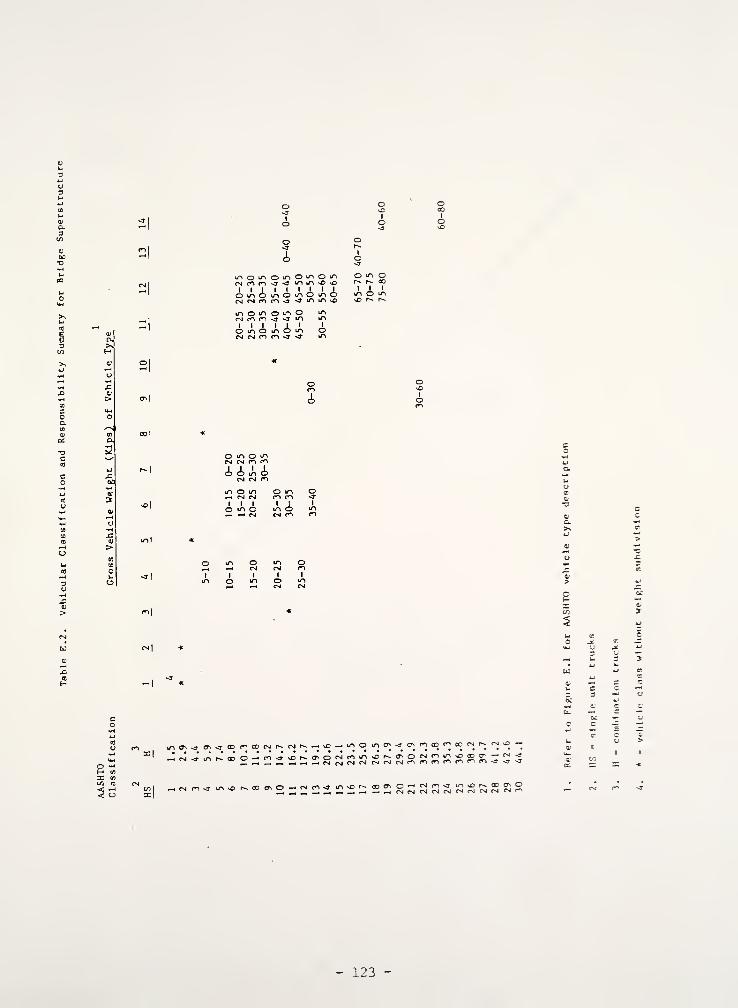
2|
o
O
3
in O m o in O in o inrj m m -» -y m in <£> \r>
i i 1 ' J. ' JL I XO in o m O in O in o
in O in O in O mr-a fi m .* -3 in in
I I I I J I I
O in O m o in On <m ri m-j < m
o m or^ r- 00
1 1 Imom\E> r~ r~
col
oIo
r-l
^1
o m O inPsJ rsi m r-i
io l ir-J (^ en
in O m o in-* r^j rsi r-
1
A1o 1m 1O i
*n— r-J cm co
ml
a
3O
c>
»l
m|
— — r^
Xu>
of-=
<N|
-I
u. —en
c c
irt 3\ ^ ^JOD'^OONP^N r^_. so —iiAO^lC-^0>n(D^C0NSN>0— csi^mr^ooO— m^*or-c*o<^cim^i^cr-0^^in.
;
£«'!r— <^-r
-<N n -j iao — cn:
- 123 -

CO
u3H
oH
2
25.00
21.88 -
18.75 "
15.63
12.50
9.375 _
6.250 -
3.125
0.0000.000 5.000 10.00 15.00 20.00 25.00 30.00
AASHTO HS TRUCKS
Ficure E.2. HS and H Trucks Correlation
- 124

Input
±Move Vehicle Across
the Bridge
Calculate Equiv.
HS or H TruckValue
ikL
Calculate Moment at
Critical Points
)iL
Turn Vehicle AroundIn Order to CrossBridge from Other
Direction
>
^L
Output
Figure E.3. Flow Chart Illustrating the Data Generation for the
Correlation process.
- 125

all bridges built in Indiana can be grouped as follows:
(a) Reinforced Concrete Slab
(b) Prestressed Concrete I-Beam
(c) Prestressed Concrete Box-Beam
(d) Steel Beam
(e) Steel Girder
For the purpose of incremental cost estimation for each of the bridge
types, a combination of the representative method and semi-statistical method
was used to develop appropriate cost distribution functions [39]. This
approach required selection of representative bridge structures and a detailed
incremental analysis was performed. The sample bridges were selected from
Indiana Bridge Inventory files.
Table E.3 shows the selected bridges and their characteristics that were
considered representative of respective bridge types constructed in the base
period.
Variation of_ Structure Width with Live Loading
Structure width for different highway categories was selected to be com-
patible with the width of the approaching highway as specified in AASHTO
Manual [1]. The FHWA study [9] assumed a constant width for all classes ot
vehicle. The Wisconsin study [48] assumed a distinct cut-off point between
the basic vehicle and the rest of the design vehicles. In this study, the
width of a bridge from curb to curb was proportionally reduced according to
- 126 -

T3O CtH ooU •H0) CD
Pi CD
Q01
COCO
m 4-1
CO >~N
o> o co-
4= o4J co
4-1 00c •H o>
•r-l C 1—
1
D ^—
'
13o>
i-i CO
o c3 cfl
i-i ai-i COCO
C ino oo
•
CO oCD 200ai-i
u /—
^
PQ •
4->
i—l 14-1
CO •
CJ X. CT*
1-1 V COP< 01 \-^
^ QH ct]
0)
en wO <
o o o o oCM CM CM CM CMco CO CO CO CO
Dd a » ffi PC
o CN 0000
ooCM iO
COco
iOCO en
in
co CM 00 U~l o~* <• CO r~ mr~ UO o co f—
i
o^ CO CM o> <r<?* <r -3- 1—
1
-a-
CO 00 O o> on
CO
O
CO
•r-l
U01
•u
ocd
uCO
6en
w0)i—
i
.oCO
H
01
H0)
00-ai-i
u03
XICOi-l
COS
0) CO
4-1 CD s01 pa rt1-1 01
o X pqc o 1
o na Mc_> 1-1
T3 TJ CD
-a 0) 0) B "001 CO CO CO l-i
o CO CO 01 -W>-i CD 01 ca oo u uIW 4J 4-1 i—
1
I—l
CI CO CO O) 0)
1-1 OJ 01 0) 0)
CD V-t 1-1 4-J 4-1
a; ex, 0- CO CO
- 127 -

size of design vehicles.
Table E.4 presents the variation of bridge width for different design
loadings and for different highway categories. The relationship between
design vehicles and observed vehicles as shown in Table E.2 was used to estab-
lish the variation of bridge width for different design loadings.
Distribution Between Highway and Waterway Crossings
Since the cost of substructure of bridges constructed over waterways tend
to be more than bridges constructed over highways, a weighing was performed to
adjust for this distribution based on data on all bridges built in Indiana
within the base period, as shown in Table E.5. Within the base period only a
few new or replacement bridges were constructed on local roads. An estimate
was therefore made for bridges on local roads on the basis of information from
neighboring states.
For highway crossings, the vertical clearance of bridge piers was reduced
proportionately of the required vertical clearance of the design vehicle.
This proportionality assumption was found to be reasonable on the basis of
actual computations. Vertical clearencs associated with design vehicles are
10 ft for H3; 12 ft. for H5 and HS5; and 16 ft. for H10 through HS 20 [48].
Allocation Factors
Allocation factors were developed for the major structure cost items
listed below:
(a) Superstructure
- 128 -

oCOinX
O O-3-
-3en
00
oc/3
re
-3"
-3-o-3-
o-a-
00-3-
ai
a.
ooc
CO
ohJ
oHrcco
X>
CO
00
COEC
O<3-
O
co
<n-3-
ooco
o
o-3"
co
CO
co
Oco
OCO
oro
00
-3"
-3-3-
O-3-
CO
00cHCO
o
c0>
MCU
cmCM
a;
-ac:=>
x-a
OCM03
-3-
-3-o-3-
o-3-
-3-
cooo-3-
•H 1/1
5 f-H o CN o <• o <rffi ~3- -3 <r CO CO -3-
CU
00
•
T3T-l O
o
M .—
(
O CN o <r o -3 u03
in
-3- -3- CO CO -3 a.
uoCO
CU-a
ffi ro 00 < o 00 oCO CO CO CM <r u
o
x:4-1
-a
cu
oo
•H
03
wa;
XI«
ml CO 00 <J- o 00 ok| co CO co CO CM -3"
u
e PL,
0)
4-1 oCO
4-1
>v CU CU u00 4-1 4-1 >^CO CO u CU
>v 4-) 4-) >. CO<4-4
CUcB CO CO M T3 s^ 4-1
3 1-1 rH w C 01 ffl 0) c 4-1 01
X! 0) CO CU CO 4-1 E 4-1 O C T3 ^ CU
60 4-1 M 4J X CO -H CO o 3 CO 4-1 UH c 3 c u 4-1 W 4-1 01 o o T-l 4-1 •
I 1-1 pi M 3 CO pM C/3 CO C_> Drf U CO r—
(
- 129 -

0360c1-1
03
03
OUCJ
/"\
>. B-S ft
CO ^-^ 60
£ (0
C•H
<u
g03 o LO o o o
u U3 CN —
i
m r- vort 0) O3 4-1
<0
S-4
•u ^cco
>> s~^
« 8-S 03
s N ' 60XI c60 >^ •H•H cfl U3 o in o o o33 1
to
O00 oo m co *
C M MUJ •H u0) Xs4-1
0)
« H C
^-CO
uto
X &5 3 u >-. CO
•H Pd p t-i T34-1 1 1 CO C3 <JJ 01 OXI u 4J •H OT-l CO to )-i 01
u u 4-1 P-, CO4J 03 03 1 1
03 l-l lJ Q> <U ,H•H 01 0) 4-1 4J CO
o u 4-J CO to Oc c 4-1 4-1 OH M 00 00 .J
w0).-I
XCO
H
- 130 -

(b) Piers, Abutments and Spread Footings
(c) Piling
(d) Excavation and Backfill
(e) Railing
(f) Drainage Pipes
(g) Miscellaneous Items
The development of each cost allocation factor was based primarily on the
effects of load and width requirements of the design vehicles.
Superstructure Cost Factors
The allocation factors for superstructure construction costs were
developed through the incremental design method discussed earlier. A series
of hypothetical superstructures was designed and cost estimated with various
design load increments and design standards specified in the AASHTO Manual
[1]. In the design procedure the same materials were included as used in the
original design of a sample bridge considered in the base period. The steps
taken to obtain the superstructure cost factors were as follows:
1. The actual design drawing, plans and bid information for the five
representative bridge types shown in Table E.3 were obtained from the
Indiana Department of Highways.
2. Computer programs were used to determine the following information for
each design loading.
Slab Bridge: Negative and positive moments at critical points.
- 131 -

Prestressed I-Beam: Strand pattern at midspan area of steel for
main reinforcement.
Prestressed Box-Beam: Strand pattern at midspan area of steel for
main reinforcement.
Steel Beam: Beam weight
Steel Girder: Beam weight
There were 10 different design loadings and a total of 50 computer runs
were made for 5 bridge types. The original characteristics of these bridges
that were independent of the size and weight of design vehicles were retained
as much as possible.
3. Bids for each sample bridge were analyzed and the unit costs of the three
lowest bids were averaged out. Any items that were considered unreason-
able were discarded and the engineer's estimate used. It was found that
the total cost of superstructure for the sample bridges under full design
loading (HS 20) was close to the cost estimated from the computer program
used in the study. This was due to the fact that bridge characteristics
were kept almost the same as originally built and that there was only a
small variation in bid prices. The total cost of superstructure under
full design loading calculated was set equal to the total cost of exist-
ing superstructure. The ratio of the actual cost and calculated cost was
then applied to all subsequent cost estimates associated with different
design loadings.
4. The unit cost per square foot of deck surface was obtained for each type
132 -

of bridge under each design loading. These unit costs were then updated
to 1983 dollars using appropriate cost indices. Table E.6 shows the unit
cost per square foot for superstructure by design loading and by bridge
type.
5. The total deck, areas constructed for different bridge types and for dif-
ferent highway classes during the base period were obtained from the
bridge inventory files of the Indiana Department of Highways and a sum-
mary of this information is presented in Table E.7.
6. Total deck areas were multiplied by the unit cost to give the superstruc-
ture cost factors for each highway class. The resulting factors are
presented In Tables E.8 through E.12.
7. As mentioned earlier, a semi-statistical approach was used in combination
with the representative bridge method to arrive at the allocation func-
tions. A least square analysis was performed on the results of the
incremental design analysis. It was found that a parabolic equation of
the form, a + b\|X, where a and b are constants, provided the best fit
2with a r = 0.96 ± 0.02, for all highway classes. Figures E.4 through
E.8 present the plots of percent of total superstructure cost versus
AASHTO loadings obtained from the regression equations.
Substructure Cost Factors
Substructures are structural elements of a bridge that support the
superstructure. Typical substructure elements are piers, abutments,
piles, and spread footing. An accurate design of piers, piles and other
substructure elements in a true incremental context is complicated due to
133 -

o oOJ co •
(X en co
>. pd CM
CMOinCM
CNI
CM
CO
CMco co
00C•HXIcr)
OkJ
OHHIen
cfl
CD
4Jrf LTl
o encu PGn4-1
O o4-1 CM(JM a
o
oo
o^
CSI
CM
co
OCM
o<n
oo
00-3-
oCM
ON
in
ONin
ON
CM
00
ONCM
00
CM
COCM
CO
CM
CM
CO
in
oCO
-*MD
CM
inoo
CMCM
CM
oCO
en
4->
CO
Ou
c
0)
fj
34JCJ
4-1
co
i-j
0)
ex3en
<u
00-aH
UJ
<v
H
CO
l-c
a)
cu
co
uco
on
co
oo
cp
in
co
ro
i
—
CM
m
inCM
00
o
co
com
CMCM
oCM
CO
CO
CM
CMCM
COCM
r^a^
CO 00 T—
l
r~-
o r- r-. O• • • •
o <r in CO
BCD CO
a. e 0)
:>> CO pa
H <u B Vj
pa co rH H cu
0) XI <D 01 0) T300 CO X M CD (1) >-l
o r-H o 14J 4.) -H
•H to oa M CO CO OMPQ
co
4-1
o.1-1
uuco
1)
T3
>J
O
wa.'
u3oo
O4-1
uCD
14-1
A
- 134 -

u~i
-H CO 1
•
CO -O 1 r~-
O CO|
vOO O c^-J orf o
oo
enooo>
Iooo
CO
01
u<
CI
0)
nID
00•oH>-i
03
WOJ
rHXCO
H
C^ >, O—
<
CO •
c X) mH OJ c O
4-1 o r--
XI CO u i r*»
01 C 4-1 01 : c^4J o CO COci T-l
3 4-1
Ij CO4-> CJ
en •r-l
C y-i Oo •H ^Oc_> CO >v •
CO Vj > encO 0) CO
j
CN1—
1
H 4-1 Bi
r-4-1 u CO •H i r-.pt< 4-1 M e^
• >N CO PUi
a" CO 1
CO 3X00 0)
CO H 4-1 1
<u ffi CO1u 4-1 1
< CO i
u rHI *
X 01 COo 4J uOJ a 3o M Pi .
HCO
4-1 0) i
o 4-1 :
H CO
4-1
COu cOJ co ! *4-1 Xc u !M 3 i
o
Om
~o
OO
ooo
ONCMv©CM
oen
r-oo0000
oo>
•
o
OCN
•
vOr-.
cnen
ou-i
•
en
o
LTl
enoo
CNo
CM
o o00 en• •
<r vDvD o<r vO<r r»-
2* w5* 03
01 w S a!00 as <Q -J ,-J wTJ 0)
5W U w qW adh a. X CQ w
u >^ J o 1 H H i-1
03 H CO 02 M CO CO o
o•Hu0)a.
0)
toCO
XI
0)x4J
c•Hx
HI4Jo
24-1
CO
coo
<D
X4-1
OJoo-a•H
X
135 -

-r-< CM
oH
u oA3 —
I
r-t CO
a —o x
o
W
u
s.
- 136 -

uto
ca
u01
a-
I
- 137

oo
oJoH
.O WX
c —
'
-I = I
oo
oU
I/)
uo
J3CO O
H
- 138 -

oHIE
OOO
Ooo
t-H
H
- 139 -

00c
O MlJ
Si
35in
to
o. 3.
u.
o
140

HOu
HOHP-,
OHZwuw
1 20 .
105.0
90.00
75.00
60.00
45.00
16 + 12.49 V X
D Data From Incremental Design
o Data From Regression Analysis
30.00
15.00
0.0000.000
_i_
5.000
j_
10.00 15.00 20.00
AASHTO HS LOADING
25.00 30.00
Figure E.4, Percent of Total Superstructure Cost vs. AASHTO HS
Loading for Interstate Urban Bridges
- 141 -

,"1 .11
HOu-J<HOH
OHWuw
105.0
90.00
75.00
60.00
45.00
Y = 31.02 + 14. 72 si X
n Data From Incremental Design
O Data From Regression Analysis
30.00
15.00
0.000. I -L _0.000 5.000 10.00 15.00 20.00
AASHTO HS LOADING
!5.00 30.00
Figure E.5. Percent of Total Superstructure Cost vs. AASHTO HS
Loading for Interstate Rural Bridges
- 142

HOuhJ<3HOHfnOH!SWuPiwP-,
20 .
105.0
90.00
75.00
60.00
45.00
30.00
15.00
0.000- _L _L
40.72 + 12.87
Data From Incremental Design
Data From Regression Analysis
_L _L
0.000 5.000 10.00 15.00 20.00
AASHTO HS LOADING
25.00 J0.00
Figure E.6. Percent of Total Superstructure Cost vs. AASHTO HS
Loading for State Primary Bridges
- 143 -

.120.0
HooOCJ
J<HOHPuOHZWUwPL,
105.0
90.00
75.00
60.00
Y = 42.43 + 12.59 W X
45.00 _
D Data From Incremental Design
° Data From Regression Analysis
30.00
15.00
0.000.
0.000
_L _L _L _L
5.000 10.00 15.00 20.00
AASHTO HS LOADING
25.00 30.00
Figure E. 7
.
Percent of Total Superstructure Cost vs. AASHTO HS
Loading for State Secondary Bridges
- 144 -

HO
HOHfnOH
uw
120.0
105.0
90.00
75.00
60.00
45.00q Data From Incremental Design
Data From Regression Analysis
30.00
15.00 _
0.000-
0.000
X5.000 10.00 15.00
_L
20.00 25.00 30.00
AASHTO HS LOADING
Figure E.8. Percent of Total Superstructure Cost vs. AASHTO
Loading for Bridges on Local Roads
145 -

the effect of other loadings such as ice, thermal stream flow, wind and
so on [42], These loadings affect the design almost Independently of
vehicle characteristics. Furthermore, the effect of these non-traffic
loadings on bridge substructure is difficult to identify. It should also
be noted that soil condition and loading capacity of the soil greatly
influence the substructure design. Consequently, as in the 1982 FHWA
cost allocation study [9], the soil mechanical properties of the sample
bridge and hypothetical bridges designed on an incremental basis were
assumed to be identical and the loading capacity of the soil was assumed
to vary linearly and therefore, proportional to the load placed upon it.
The 1982 FHWA study [9] designed piles based on the assumption that
pile length is proportional to the applied load. Thus, pile length was
reduced proportionally as the loading was reduced. The piers for the
hypothetical bridges were assumed to have the same general configuration
as the sample bridge. The stem of the pier and of abutment was varied
according to the road width variation. The wing wall and width were
maintained constant.
In the present study, individual cost responsibility factors were
obtained for piles, piers and abutments. Other components of substruc-
ture, such as pile cap, were assumed to be non-attributable cost. The
pile length was assumed directly proportional to the applied load. It
was found that 75% of the total applied load was dead load and 25% was
due to the live load. Hence, 75% of the cost was assumed to be non-
attributable cost and the remaining 25% was distributed according to the
live load. The cost responsibility factors for piles are shown in Table
E.13. The stem of pier and abutment was varied according to the road
- 146 -

o in mo 00 in r*» CN
enCO
o•
en .
—
I
•
33
o00
Xcn
oin m
CN•
Oo•
o I"* l"»
<t in 00 <*»
in r^ >—
4
0~i•
o oom
000000
CO
Vj
o4Jo
to
•u
03
o
60c
P-,
CO 1—
1
01 coa. 33P~>H00 inC •-H
•H *•aCO
o•J oo 1—
<
H XS3CO
3inCOre
o in m*jO in CN r^CO r- •~* 00
sl
si
o <r <r
o m o mCO r-~ i—
i
00• • •
o^ CT>
o CN <No in vO .—l
CN r-~ o 00• •
en
•
o CN CO00 m vO CN.—
1
r~» o i—
*
• • 00•
O ~3- mo m cn -4-
w—1 r*. O 00• •
•
r-~ r»o O O
v£> in CN r-»
r~ O r-
01
CO
H
^ C2 ^uCO
CO O CJ ocu oM e IK
^! o Vj O u oo Mo O o c O
4-1 s-s 4-1 w 4J
3 B^? u o 1—1 CJ
> in CO in CO T-( CO
O r- to CN h-, Pu fn
- 147 -

width variation. The cost responsibility factors for pier and abutment
are shown in Table E.14.
Excavation and Backfill Factors
The FHWA study [9] proportioned the cost of backfill and excavation
according to the deck width. The smaller the width of the bridge, the
lesser the amount of backfill and excavation. The same procedure was
used in the present study and therefore the factors are the same as in
the case of pier and abutment.
Drainage Pipe Factors
Although most of the previous cost allocation studies assumed the
cost of drainage pipes to be non-attributable cost, it can be argued that
the size of drainage pipes is related to the quantity of runoff which in
turn is related to the width of the deck surface. As the deck width can
be related to vehicle width, drainage pipe can be considered to be an
attributable cost. The same approach as that taken for pier and abutment
can be applied here and therefore the drainage pipe cost factors are the
same as in the case of pier and abutment.
Railing Factors
According to AASHTO specification [3], the minimum railing height is
2'-3". Railing members are designed for a moment due to concentrated
loads at the center of the panel and at the posts of the railing for PL/6
where P is the concentrated load and L is the post spacing. The common
148 -

omCO3S
OCNco
CO
O4-1
CJ
co
4-1
en
o
COaa
0)
a.>^H ooo »—
<
c co•H ncT3cfl
OJO inH to
pa ffi
c/)
3>. oX> CN
pacn
Ij
o4-1
O incfl
i—
i
fc x:
4-1
cn
O oU .—
i
o m moo
ooCO o>
o in in m 00 CNI
on ON 00 00 00 a\
CNI
00 00moo
m CNI
00CNC^
oOn
oas
inon
mon
moo
moo
00oo
oooo
CNon
CNI
ON
c0)
6
CNI sD in mb°l 00 00 00 i-n CN cnaa| • • • • 00 oo
3J}<-accfl
n CN O m m «N roX'| OO 00 00 r^ 00 00
CO1-4
CD
wcu
.H
cfl
H
B4-1
cn
>^CO
cfl
3J=001
cfl
4J
cn
U —Icu cfl
4-1 uC 3l-< OS
cnu CCD cfl
4-) XC nM 13
cfl -H4-1 Uco a*
Mcfl
Co
cfl U4-1 <D
CO CO
CD
a -a3 CO
o o
4-1
CD
>~, CD4J Ut4 4-1
C_J CO
- 149 -

cost portion was determined by using the cost related to the smallest
vehicle loading in the formula. This portion was found to be 25% of the
total railing cost. The remaining 75% was distributed according to the
gross vehicle weight. The cost responsibility factors for railing are
shown in Table E.15.
Miscellaneous Items
Miscellaneous items consist of those costs that are independent of
vehicle size or weight and they include such items as engineering ser-
vices, installation of traffic control devices, landscaping, and so on.
These costs were thus considered to be non-attributable and distributed
among all vehicles as common costs in proportion of their respective
vehicle-miles of travel.
Allocation of Cost-Responsibilities
Appropriate cost factors were developed for each of the structural
cost components, and these cost factors were expressed in terms of AASHTO
vehicle types. The next step was to combine these cost items and relate
them to the appropriate respective vehicle classes considered in the
present study. The steps involved in this procedure are listed below:
1. The VMT of each of the AASHTO vehicle types was obtained by
using the correspondence matrix for matching AASHTO vehicle
types with study vehicle classes shown in Table E.2.
2. The common portion of the total cost was distributed among all
AASHTO vehicles according to VMT.
150 -

O in mO
j
00 in CM r»co
1 o CM t—
1
COco »—i
• • •
X .
^H
o,
o oCM • CM m in oCO r^ CM r~- •
33• • ^H
in o .—1 ^H•—
i
<r in vO 00co , m CM m •
Sti 1
• •
o o m mCM
IO m r-
1
vOK| «* CM <a- vO
G.>>H00
to|
3dCO
omCM
CM
CO
CMCM\40
o CM CMo in r-i ^CCO CM CO m
05
o4-1
oco
fa
4-1
o
00c
XIrs!
O
OHPSto
3mlCO !
W!
o r-- r-o in O mCM CM CM <r
00
a
a'
o vD COm oo vOCM i—< <r
• • •
o co COm O mCM i—
i
CO• •
co
•
o CM CMin vD ~HCM O co
fa
H
S en
^-N c £> oCO o O ufa iM 6 fa 0C^ o u O u c ^^^ a o o H O
ij s-s 4-1 .H 4-1
s 8~S o o •H U> m <0 in (0 (0 cfl
U CM fa r~ fa ei fa
- 151

3. Subsequent incremental costs were then allocated to appropriate
AASHTO vehicle types.
4. The total allocated costs for each of the AASHTO vehicle types
were assigned to the study vehicle classes using the correspon-
dance matrix established in Table E.2.
New Bridge Construction
If a bridge was constructed during the base period specifically on a new
alignment, it was taken to be a new construction. All new construction costs
within the base period were analyzed in terms of cost items and grouped into
different highway classes. Table E.16 shows the percent distribution of new
structure construction costs by cost item and by highway class.
Bridge Replacement
Bridges are replaced due to the deficiencies of the original structures.
Consequently, the FHWA study [9] treated bridge replacement costs differently
from new bridge costs. A structural sufficiency rating was used to determine
the relative contribution of each factors which were responsible. Costs were
assigned to vehicles based on the sufficiency rating components. Deficiencies
in original structures may include low load carrying capacity, inadequate lane
width, fatigue worn components, and inadequate overhead clearances. However,
the federal study simplified the allocation procedure by considering only
load-deficiency related replacements. It further assumed that losses or
inadequacies in load-bearing capacity are entirely attributable to heavy vehi-
cle use. Because of the difficulty of determining age and environmental fac-
tors on load bearing capacity, it was decided in the present study to use the
- 152 -

Table E. 16. Percent Distribution of New Bridge
Construction OorL by Cost Item and
by Highway Class
Interstate State
(Rural & Urban) Primary
Superstructure
Substructure
14% 17%
StateSecondary
26%
LocalRoads
25.06
Piers and Abutments 1.9% 8% 6.4% 6.29
Piling 0.3% 1.8% 2.9% 2.87
ExcavationBackfill
and0.7% 6.6% 6.6% 9.43
Drainage 0.02% 0.01% 0.02% 0.05
Railing 0.41% 0.46% 5.8% 5.59
Miscellaneous 79% 64% 48% 50.71
Total 100% 100% 100% 100%
- 153 -

same approach as used in the new construction but with different distribution
of cost components. A replacement project would not Involve much excavation
rk, but it will require removal of the existing structure.wo
The percent distribution of component costs for replacement project was
determined by analyzing the itemized cost files from the IDOH. The resulting
cost distribution by cost item and by highway class is presented in Table
E.17.
Bridge Rehabilitation Cost
Bridge rehabilitation costs included cost of widening, deck repair and
partial replacement of structural components. Bridge rehabilitation costs are
different from bridge maintenance costs, because rehabitation work is not done
routinely and it is normally more expensive than routine maintenance.
Many studies combined the rehabilitation costs with replacement costs.
Other studies assumed rehabilitation costs to be common costs. In this study,
the cost responsibility factors for bridge rehabilitation project were
developed using the same approach as the new construction, but with different
distribution of cost components. The cost distribution by cost item and by
highway class is shown in Table E.18. It may be noted that a large percent of
the rehabilitation cost is non-attributable cost.
Culverts
In the base period, not too many box culverts were built. Most of the
box culverts were replaced by metal pipes and structural plates. The size
the pipes is dependent mainly on the drainage requirement of the surrounding
- 154 -

Table E.17. Percent Distribution of Bridge Replacement Cost
by Cost Item and by Highway Class
Ini rrntaU; Stati1 State Local
(Rural tx Urban) Primary Secondary Roads
Superstructure 28.5% 29.5% 26.2% 27.00%
Substructure
Piers & Abutments 7% 2.6% 6.0% 5.74%
Piling 0.01% 0.6% 0.13% 1.37%
Excavation &
Backfill 9.88% 19.6% 18.6% 18.51%
Drainage 0.01% 0.10% 0.007% 0.12%
Railing 5.7% 3.2% 6.50% 6.08%
Miscellaneous 48.9% 44.4% 42.50% 41.18%
Total 100% 100% 100% 100%
155 -

Table E.18. Percent Distribution of Bridge Rehabilitation Cost
by Cost Item and by Highway Class
Interstate State State Local
(Rural & Urban) Primary Secondary Roads
Superstructure 7.60% 5.72% 19.3% 14.82%
Substructure
Piers & Abutments 0.60% 0.50% 1.9% 0.79%
Piling 0.03% 0.01% 0.9% 0.20%
Excavation &
Backfill 0.10% 2.79% 5.5% 0.55%
Drainage 2. 70% 0.008% 0.004% 0.23%
Railing 6.70% 7.70% 5.70% 6.42%
Miscellaneous 82.40% 83.20% 66.70% 76.99%
Total 100% 100% 100% 100%
- 156

areas. Consequently, it was considered a common cost. Box culvert is largely
related to the weight of overfill and the weight of overhead roadway slabs.
Therefore, all future culvert costs were assigned to all vehicle classes as
common cost.
Sign Bridges
Sign bridges were singled out because their cost responsibility is
vehicle-size related. For lighter and thus smaller vehicles, the horizontal
and vertical clearances can be reduced appropriately. A typical sign bridge
has a vehicle clearance of 18 feet and a span length of 80 feet. The pro-
cedure used by the Wisconsin study [48] was followed to allocate sign bridge
costs.
For autos (H3) and light trucks (H5) , the sign bridge geometry can be
reduced as follows:
H3 H5 HS5 H10-H20
Column 11' 13' 15' 18'
Span 48' 68' 72' 80'
Responsibility factors for sign bridges are then:
- &T^ »•"
13 + 68Q
„ 9Hi80 + 18
U,8/
HS5 i-r-if = °- 88
- 157 -

H10-HS20 g±# - 1.00
- 158 -

APPENDIX F
MAINTENANCE COST ALLOCATION
General
A particular item of maintenance cost can be classified as a "common"
an "attributable" cost. A common cost is a cost that cannot be specifically
allocated to a class or classes of vehicles, and is therefore distributed
among all highway users. For example, mowing of grass or the pick up of
litter within right-of-way can be considered as common cost. Common costs
are to be borne by all users in direct proportion to the number of miles
driven by each. Therefore, the common-cost allocator for each vehicle class
is the VMT by that class as a percentage of the total VMT by all vehicle
classes
.
An attributable maintenance cost is a cost that can be directly allo-
cated to a particular class or classes of vehicles. Attributable costs can
be allocated on the basis of weight related allocators for those items that
can be associated with vehicle weights. Some items can be allocated according
to capacity related allocators when vehicle size affects the cost.
Previous Studies
Methodologies to allocate maintenance costs used by cost allocation stu-
dies by nine states were reviewed for comparison. These nine states are Con-
necticut, Florida, Maine, Maryland, North Carolina, Oregon, Washington,
Wisconsin, and Virginia.
It was found from this comparison that there exists no universal method
for the allocation of maintenance costs. This is especially true for the
159 -

costs (pavement, shoulders and bridges) that are related to the weight of
vehicles. The selection of cost allocators is based on various assumptions
and reasonings. A majority of these states used ESAL as the cost allocator of
pavement related maintenance costs. It seems however that the U6e of
vehicle-miles of travel (VMT) has been accepted in most of the allocation stu-
dies for allocation of the common costs.
Allocation Methodology
Routine maintenance activities are classified into the following major
groups:
1. Roadway and shoulder maintenance
2. Roadside
3. Drainage
4. Bridge
5. Traffic Control
6. Winter and Emergency
7. Public Service
8. Others
Roadway maintenance consists of activities such as patching, leveling,
and sealing of cracks and joints. The associated pavement damages are con-
sidered to be caused either by climatic conditions or by the interaction of
climate and the weight of vehicles.
For the purpose of allocating roadway maintenance costs due to traffic
and its interaction with weather, a procedure was developed in the present
study to separate the load-related and non-load-related effects, as discussed
later in this section.
- 160 -

In the case of shoulder construction, use of capacity related cost allo-
cators Is justified; however, they may not be appropriate for the allocation
of shoulder maintenance costs, because shoulder damages are more of a function
of weather and traffic. The weather affects shoulder conditions more severely
than pavements. Once constructed, functions of highway shoulders are to hold
roadway pavement in place and strengthen it. Obviously the heavier trucks
would cause more distress than the lighter vehicles. It was decided, there-
fore, to allocate the traffic-related component of shoulder maintenance costs
in proportion to the costs assigned to vehicles for pavement maintenance. In
this approach, assumption is made that the probability of using shoulders for
emergency stops is equal for all vehicle classes.
All other maintenance costs, except bridge maintenance costs, were allo-
cated as common costs to all vehicle classes because these costs cannot be
directly related to the variation in highway use by different vehicle classes.
There are seven items under bridge maintenance of which bridge mainte-
nance contract work can be judged partly to be the result of the interaction
of traffic and weather. Consequently, this part of the maintenance cost was
allocated using the approach used for pavement related maintenance costs. All
other bridge maintenance costs were considered to be common costs.
Some of the activities in the "Other" category include operational over-
head such as supervision and equipment repair and maintenance and therefore
these operational overhead costs were grouped with administrative overhead.
Administrative and operational overhead costs were allocated to all vehicle
classes in proportion to the sum of direct maintenance costs. These costs
were first assigned percentwise to the three maintenance costs groups, then,
- 161 -

allocated to vehicle classes by the cost allocator(s) of each cost group.
Data Base for Analysis
Routine maintenance costs for the state highway system were estimated
using the Routine Maintenance Records and Construction Reports. As for cost
items, Routine Maintenance Records contain only labor, production units, types
and quantities of materials used. Maintenance costs for labor and material
were computed by multiplying the labor and material units required for each
activity by separately provided unit costs. Fuel consumption data are not
found in Routine Maintenance Records, but are reported in lump sum for all
maintenance works for each fiscal year. To distribute fuel costs to each
activity, results of a previous study [36] concerning the fuel consumption
rates of routine maintenance activities was used. Routine maintenance activi-
ties that have been done by contract are found in Construction Reports file.
Procedure for Allocating Pavement Routine Maintenance Costs
The procedure for allocating pavement routine maintenance costs pursues
the same concept adopted for allocating pavement rehabilitation costs. The
maintenance expenditure items included in the computation of pavement routine
maintenance costs are shown in Table F.l.
As explained earlier in the section on allocation of pavement rehabilita-
tion costs, an actual field performance curve of a given pavement would lie
between the no-loss line and the zero-maintenance curve. The higher the level
of routine maintenance performed, the closer is the field performance curve to
the no-loss line.
162 -

Table P. ] . Pavement Routine Maintenance Activities
IDOH Code No. Activity Name
201 Shallow patching202 Deep patching203 Premlx leveling204 Full width shoulder seal
205 Seal coating206 Seal longitudinal cracks and joints207 Sealing cracks209 Cutting relief joints219 Others
- 163 -
In Appendix H, a technique is described which enables the zero-
maintenance curve to be derived by considering pavement performance curves and
Ltielr associated routine maintenance expenditure expressed In terms of average
annual routine maintenance expenditure per lane-mile. Also presented In
Appendix H is a proportionality rule by means of which the respective respon-
sibility proportions of load-related and non-load-related effects of pavement
damage can be computed.
Since the effects of non-load-related factors may be different for dif-
ferent regions (northern and southern Indiana), and pavement types (overlay,
rigid and flexible pavements), maintenance expenditure data were divided into
six region-pavement type groups. In addition, six highway classes were used
in the present study and each with a different vehicle composition. This
means that 36 routine maintenance expenditure subgroups in total needed to be
analysed in the cost-responsibility factor computation.
- 164

APPENDIX G
REVENUE ATTRIBUTION
After cost responsibilities are Identified It is necessary to examine
revenue payment by vehicle class to provide a base for comparison. The appor-
tionment was done of appropriate revenues paid by Indiana highway users to
state, federal and local governments. In particular, the user revenues con-
sidered are those which went to support highway construction, operation and
maintenance activities in Indiana.
State Highway Revenues
The Indiana system of funding of highway activities includes two major
accounts, Motor Vehicle Highway Account (MVHA) and Highway Road and Street
Fund (HRSF). The sources of revenue consist primarily of the motor fuel taxes,
registration fees, and motor carrier fees. In addition, miscellaneous reve-
nues in the nature of fines and charges are collected and deposited in the
Motor Vehicle Highway Account (MVHA). Furthermore, in recent years some user
fees and taxes have been imposed by some local governments in the form of
local option taxes. In Figure G.l is presented the current organization of
the MVHA. The majority of highway revenues in Indiana is gathered in MVHA
where fuel taxes and registration fees are the main sources of revenue. The
other highway related fund is the Highway Road and Street Fund (HRSF). A part
of the motor fuel tax and truck registration fee is gathered in the HRSF for
use in two separate accounts, the Primary Highway Fund and the Local Road and
Street Fund.
165 -

Figure G.l. Organization of the Motor Vehicle Highway Account (MVHAJ
Motor Fuel Tax
Vehicle License FeesGeneral Fund Reimbursement
for State PoliceFederal ReimbursementsDriver Court FeesReinstatement Fees
Miscellaneous Receipts
Revenue
Motor Vehicle Highway Account Fund
,
Expenses
Bureau of MotorVehicles
Indiana StatePolice
Traffic Safety
Motor FuelDivision
"
MiscellaneousExpenses/FuelTax and OtherRefunds
Highway Funds
53% Indiana Departmentof Highways
15% Indiana Cities and
Towns
Distributed in prop.j
to population
32% *— Indiana Counties
J
5% Distributed equally
30 1 Proportion tc MotorVehicle Registration
653 Proportion tc tctal
County miles
166 -
The motor fuel taxes are the major sources of highway revenues In Indiana
and they consist of three items, motor fuel tax on gasoline, special fuel tax
involving primarily diesel fuel, and motor carrier fuel tax imposed on inter-
state carriers.
Federal Revenues
Federal funds available to Indiana are generated through Federal Trust
Fund. In 1983 the revenues included motor fuel tax, tax on new trucks and
trailers, parts and accessories tax, tires and tubes tax, tax on lubricating
oil and heavy vehicle use fee. The Surface Transportation Assistance Act of
1982 and its subsequent amendment resulted in several changes in federal tax
structure. For example, taxes on tread rubber, inner tubes, lubricating oil,
and truck parts were eliminated and new tax schedules were introduced for fuel
taxes and taxes on truck sales and heavy vehicle use.
It should be noted that only that portion of the federal revenues that
was received by Indiana was considered in revenue analysis. For example, in
1983 the amount received by Indiana was $155.56 million or about 75% of the
revenues contributed by Indiana highway users to the Highway Trust Fund. The
STAA of 1982 stipulated the percentage of return to be at least 85%.
Attribution of Revenue
Each of the state highway user charges were examined separately to attri-
bute the shares of revenues to vehicle classes. In each case the revenues
attributed were equal to the amount available for highway purposes. For exam-
ple, the disbursements to the Bureau of Motor Vehicles from the Motor Vehicle
- 167

Highway Account were considered to be associated with the collection of state
registration fees and were thus deducted from the gross amount. Similarly,
the disbursements to the Motor Fuels Tax Division of the Department of Revenue
were deducted from the total fuel taxes collected. However, these expenses of
collecting and administering these taxes were not included in cost computa-
tion.
State Fuel Taxes
In FY83 total state fuel taxes collected in Indiana consisted of gasoline
tax, special fuel tax (diesel) and motor carrier fuel use tax; and the total
amount available for MVHA, HRSF and regular distribution was $314,248 million
with 81% from gasoline tax, 17% from special fuel tax and 2% from motor car-
rier fuel use tax. Considering the gasoline tax refunds and disbursements for
the Motor Fuel Tax Division and other associated expenses, the net amount
available for highway activities was $305,175 million. This amount was shared
by the IDOH, counties, cities, and the State Police. The corresponding amount
for the biennial period of 1985-86 would be $614 million.
Fuel taxes are dependent upon fuel consumption which in turn is related
to vehicle-miles of travel and vehicle fuel efficiency. The VMT values by
vehicle class for 1983 were available from the traffic count data. Fuel effi-
ciency estimates by vehicle class for both 1983 and 1985-86 were generated by
combining the figures from the FHWA Cost Allocation Study [9] with the find-
ings of an earlier study performed for the IDOH [29]. To compute fuel con-
sumption, annual VMT for a specific vehicle class was divided by its fuel
efficiency value. Gallons of fuel consumed was then multiplied by the
appropriate tax rate. It should be pointed out that percentage of vehicles
powered by gasoline and diesel were estimated from the information available
- 168 -

in the National Truck Characteristics Report [23] . For example, 1 1 .94X of 2-
axle single-unit trucks was estimated to contain diesel engines, while 99.35%
of combination trucks with 5 or more axles wouLd have diesel engines. These
estimates were made by vehicle type and by number of axles. Furthermore,
while gasoline and special fuel taxes were attributed among all vehicle
classes, motor carrier fuel use tax was distributed only among trucks with
more than 2-axles.
The same procedure was used to attribute the state fuel tax revenues for
the 1985-86 period on the basis of the estimated VMT and fuel efficiency rates
for these years. The 1985-86 VMT projections were developed using the factors
developed in connection with the Federal Cost-Allocation Study and factors
used in the studies conducted by several midwestern states.
State Registration Fees
A flat vehicle registration fee is charged to private automobiles in
Indiana, while the fees schedules for commercial vehicles are graduated by
registered weight. The total motor vehicle registration fees available for
highway related activities in Indiana in FY83 were $109.7 million, after
deducting disbursements for the Bureau of Motor Vehicles, miscellaneous
expenses and the amounts associated with dealer's fees, transfer fees and
other fees, such as fees for amateur radio. The registration fees for 1985-86
were estimated on the basis of the information provided by the IDOH and the
Bureau of Motor Vehicles. The net amount estimated to be available for high-
way purposes in the two-year period of 1985-86 is $225.8 million.
Registration fees were attributed directly in proportion of the number of
units of each vehicle class and associated registration fee rate. As men-
- 169 -

tioned earlier, a correspondence matrix was used to relate vehicles classified
by gross operating weight with registered vehicle weight groups.
Other Taxes and Fees
Other taxes and fees at the state level were $2,502 million in 1983 or
about 0.4% of the total available revenues. The majority of these fees came
from oversize and overweight permits. The rest of these fees came from vehi-
cle identification stamp fees, reciprocity fees and others. These fees were
distributed among commerical vehicles in proportion to number of units. In
1985-86 miscellaneous state fees are estimated to be $5.35 million and the
attribution would follow the same procedure as in 1983.
Local option taxes in 1983 amounted to $1,058 million or about 0.2% of
the total. In 1985-86, the estimated amount is $5.5 million. Local option
taxes are levied by counties and consist of an excise tax imposed on all motor
vehicles and a wheel tax imposed on motor vehicles that are not subject to an
excise tax. The attribution of these taxes was done by distributing the
amount in proportion of registered units of all motor vehicles.
Federal Taxes
All federal taxes were attributed according to the appropriate user
charge schedules. The applicability of each type of tax or fee along with the
effective date of implementation of each tax or fee type was considered for
appropriate vehicle classes. The factor for distributing 1983 taxes on oil,
tire, tubes, tread rubber and truck parts were obtained from the report [35]
prepared for the Federal Highway Cost-Allocation Study. The 1983 factors were
developed by interpolating the 1977 and 1985 factors given in the report. The
rate of new truck sales and associated prices were also generated using the
- 170 -

Information given in the report [35]. Heavy vehicle use fee was attributed In
proportion of number of units In each commerical vehicle class of concern.
The rates and effective dates were carfully considered in estimating the
amount of this fee.
- 171 -
APPENDIX H
Determination of Cost-Responslblllty Factors of Load-Related and
Non-Load-Related Costs In Pavement Rehabilitation and Maintenance
Cost Allocation
The procedure discussed herein follows a performance-based approach
developed by Fwa and Sinha [13]. A summary of this approach is presented in
this Appendix.
As discussed in the section on allocation procedure of pavement rehabili-
tation costs, pavement wear or damage may be represented by appropriate areas
in a pavement performance (PSI vs. EESAL) plot. In Figure H.l, the shaded
area (A + B) between curves 3 and 4 represent the total pavement damage of a
o
given stretch of pavement. Curve 3 is a hypothetical no-loss line and curve U
is a hypothetical performance curve for the pavement concerned in a situation
where no maintenance at all has been carried out.
Consider a stretch of pavement which is maintained by a particular high-
way agency with known technology, facilities, and manpower, and assume that
the efficiency of the working crew remain the same for the period of analysis.
Under these conditions it is reasonable to say that the expenditure spent on
maintaining the pavement would be positively related to the level of routine
maintenance performed. That is, in terms of constant dollars higher expendi-
ture is likely to be associated with higher levels of maintenance. In Figure
H.2, one would expect the expenditure level S„ to be greater than S2
,S,,
greater than S., and so on.
- 172 -

E->-
VOc-c-
~
I
o1-
01
N
—01
=
-D03
CTJ
01
«Et:
^ >
-j az _01= -
> c
-J u3 -
-
_
—
COQ.
- 173 -

eo
05
> £ ?03
_l « —
1
CO
Oc o ccd o «3cz CO C03 CO CUM < +
c(5
2 tureMai
OS
114-» <U -M3 O. =3O X Occ UJ CC
CO
<COLUW
3!
-
>l-i
r'-
ii
-r*
«3lZ
U-l
uc*
•""*
-1
ca •
E X- a> •_
a na. -j—
<
=c—
r* c—
1
-_
3 cX
Cfl
i.
ej —
'
>- ijso r•^ w—
<
-•
q-o
<j o—
)
uu ca —£ -)
J o*" Xu —VD <
COCL
u3
174 -

Performance curves based on Indiana design equations vary with the fol-
lowing factors: type of pavement, region, terminal PSI, materials and traffic
Indiana material and regional factors estimated In an earlier work done at
Purdue University [6] were used for this purpose. Cost-allocation analyses
would be performed by highway class and type of pavement. For each pavement
section on which a rehabilitation had been performed during the base period,
performance curves corresponding to Indiana design equations and actual field
performance were developed.
The Road-Life Records of the Indiana Department of Highways contain the
following information for each route of the State Highway system:
1. Pavement type
2. Pavement thickness
3. Pavement age since the time of major improvement
A. Layer material characteristics, and
"3. Construction costs
Pavement roughness measurements on Indiana State Highways since 1979 are
available from JHRP tapes at Purdue University. These roughness measurements
can be related to PSI by using relationships established for Indiana in previ-
ous studies performed at Purdue University [30,31]. The relationships derived
for different types of pavements are summarized in Table B.l.
For a given pavement, knowing a PSI value and the corresponding cumula-
tive ESAL, a point on the actual performance curve of the pavement is
obtained. This procedure may be repeated for other points of time at which
- 175 -

Table K.l. Relationship Between Present Serviceability Index (PSI)
and Roughness Number (RN)
Pavement Relationship
Asphalt PSI = 3.94 - 0.00072(RN)
Overlay PSI = 4.37 - 0.00174(RN)
Jointed Reinforced Concrete (JRC) PSI = 4.69 - 0.00141(RN)
Continuously Reinforced Concrete (CRC) PSI = 4.40 - 0.00070(RN)
JRC & CRC (combined) PSI = 4.58 - 0.00114(RN)
176 -

data are available. Field performance curve of the pavement may then be plot-
ted, and the area between this curve and the no-loss line, ie. area (A+B), may
be computed.
The annual routine maintenance cost per lane-mile of a pavement section
was obtained by dividing its annual routine maintenance expenditures by its
total lane-miles. The annual routine maintenance expenditures over the base
period were considered to compute the average maintenance cost for the highway
section under consideration.
Routine maintenance information is documented by highway section which is
defined as the portion of a highway that lies within the boundaries of a
county. Highway section was therefore chosen as the basic unit of analysis in
the present study. When a pavement section contains more than one roughness
measurement, a weighted average of area (A+B) was calculated using the lane-
mile of each roughness measurement as the weighting factor.
For a stretch of pavement with more than one highway section, the zero-
maintenance curve of the pavement was derived by plotting the areas (A+B) of
these highway sections against their respective average annual routine mainte-
nance expenditure per lane-mile. A least square line was then fitted to the
data points. The intercept of this line with the (A+B) axis gives area (A+B)
of the zero-maintenance curve of the pavement under consideration.
The next step involves the computation of load-related and non-load-
related responsibility factors using proportionality assumption. Figure H.3
assumes that the interaction effects is composed of two components, namely the
load-related and non-load-related parts. Proportion a is equal to > . „^—o
which could be computed for a given stretch of pavement with the procedure
- 177 -

Load-related
effects
Load-related
effects
Non— load-related
effects
Non— load-related
effects
(a)
Interaction
effects
j
a
(b)
Figure H.3. Schematic Diagram Showing Load-related and Non-load-related Effects Responsible for Pavement Damage
178 -

described in preceding paragraphs.
Knowing proportion a, it is possible to calculate proportions b, c and d
by making the following proportionality assumption:
b+c+d a+b+c+d
a+b+c a+b+c+d
(H.l)
(H.2)
Equation (H.l) assumes that for a given 'pure' load-related effects (pro-
portion a), the share of load-related effects in the remaining non-load-
related and interaction effects is directly proportional to the share of
'pure' load-related effects in the overall effects (a+b+c+d). Similarly,
equation (H.2) assumes that for a given 'pure' non-load-related effects (pro-
portion d), the share of non-load-related effects in the remaining load-
related and interaction effects is directly proportional to the share of the
'pure' non-load-related effects in the overall effects (a+b+c+d).
Solving for d using equations (H.l) and (H.2), it gives:
1 - \ l-(l-a)2
(H.3)
Proportions b and c may then be determined from solving equations (H.l)
and (H.2). The total responsibility proportion of load-related effects is
given by (a+b) and the total responsibility proportion of non-load-related
effects by (c+d).
Applying the procedure described in this Appendix to Indiana highways,
the resulted proportional responsibilities of load-related and noa-load
179 -

related factors for different regions and pavement types are summarized in
Table H.2.
The regional effect changes gradually from northern to southern Indiana
and there exists no distinct boundary between them. For the present cost-
allocation study, the two regions were defined as shown in Figure H.4.
- 180 -

Table U. 2. Proportional Responsibilities of Load-Related and
Non-load-related Factors in Indiana PavementRehabilitation and Maintenance Cost Allocation
Northern Indiana Southern Indiana
Factor Flexible Rigid Overlay Flexible Rigid Overlay
Pavement Pavement Pavement Pavement
Load-Related 0.87 0.66 0.80 0.98 0.70 0.98
Non-Load-Related 0.13 0.34 0.20 0.02 0.30 0.02
- 181 -

Figure H.4. Northern and Southern Regions tor Pavemunc ost-Al locat ion
NORTHERNREGION
182 -

APPENDIX I
TABLES OF COST-RESPONSIBILITY FACTORS
- 183

Table 1.1. Pavement Construction Cost-Responsibility Factors
(a) Pavement Construction Cost-Resp .(%) for 1983
Vehicle Int. Int. State State County CityClass Rural Urban Primary Second. Roads Streets
1 8.667 11.869 11.564 5.560 5.069 5.3762 27.239 36.848 40.652 22.174 27.215 23.2893 2.057 2.806 3.919 4.919 14.699 4.1244 0.269 0.376 0.189 0.211 1.683 3.4305 0.657 0.537 0.340 0.176 0.273 0.1676 0.411 0.607 1.640 1.876 7.622 2.7407 0.459 0.577 1.392 2.120 0.646 0.3798 0.036 0.192 0.142 0.088 0. 0.9 0.226 0.179 1.484 0.603 0.019 0.015
10 0.066 0.042 0.091 0.234 0. 0.12011 3.619 2.117 1.122 2.840 3.845 2.78512 54.202 41.641 36.157 57.711 34.465 56.60013 1.857 2.048 0.772 0.660 2.945 0.72114 0.233 0.160 0.537 0.829 1.520 0.252
(b) Pavement Construction Cost-Resp. (%) for 1985/86
Vehicle Int. Int. State State County CityClass Rural Urban Primary Second. Roads Streets
1 8.620 11.869 11.556 5.560 5.053 5.3662 27.089 36.848 40.609 22.144 26.368 22.8843 1.989 2.806 3.790 4.736 11.646 3.2204 0.261 0.376 0.184 0.205 0.381 0.8045 0.653 0.537 0.340 0.175 0.263 0.1636 0.406 0.607 1.594 1.821 6.812 2.4497 0.462 0.577 1.399 2.123 0.934 0.5408 0.036 0.192 0.142 0.088 0. 0.9 0.222 0.179 1.484 0.615 2.473 1.02510 0.067 0.042 0.092 0.235 0. 0.18211 3.634 2.117 1.129 2.852 3.913 2.82412 54.465 41.641 36.364 57.957 36.099 59.31713 1.861 2.048 0.775 0.659 3.028 0.74414 0.234 0.160 0.541 0.832 3.030 0.481
- 184 -

Table 1.2. Shoulder Construction Cost-Re6ponsibility Factors
(a) Shoulder Construction Cost-Resp .(Z) for 1983
Vehicle Int. Int. State State County CityClass Rural Urban Primary Second. Roads Streets
1 7.202 10.217 10.432 5.467 3.162 3.6472 22.647 31.726 36.701 22.494 16.977 15.7993 1.790 2.379 4.491 6.011 12.393 3.3064 0.462 0.834 0.523 0.851 1.788 3.1725 0.590 0.502 0.330 0.181 0.230 0.1346 0.415 0.627 1.795 2.123 9.770 2.5357 0.522 0.666 1.020 1.597 0.828 0.5378 0.032 0.179 0.138 0.094 0. 0.
9 0.229 0.174 1.637 0.011 0.024 0.01410 0.070 0.044 0.077 0.172 0. 0.14111 4.099 2.434 1.346 2.901 4.928 3.26312 59.353 47.430 38.908 56.953 44.177 66.31113 2.324 2.602 2.019 0.680 3.775 0.84514 0.263 0.187 0.583 0.466 1.949 0.296
(b) Shoulder Construction Cost-Resp .(%) for 1985/86
Vehicle Int. Int. State State County CityClass Rural Urban Primary Second. Roads Streets
1 5.368 8.035 8.055 3.258 3.258 3.7222 16.868 24.946 28.306 12.974 12.974 14.8223 1.542 2.459 3.412 3.724 3.724 3.7444 0.242 0.405 0.202 0.202 0.202 0.1865 0.506 0.471 0.306 0.138 0.138 0.1396 0.402 0.814 2.190 2.161 2.161 1.6597 0.569 0.774 1.921 2.520 2.520 2.9638 0.028 0.168 0.128 0.069 0.069 0.0699 0.220 0.241 2.038 0.729 0.729 0.56010 0.082 0.056 0.127 0.279 0.279 0.27111 4.478 2.838 1.551 3.385 3.385 3.28912 67.114 55.834 49.957 68.794 68.794 66.85613 2.293 2.745 1.064 0.782 0.782 0.76014 0.289 0.215 0.743 0.987 0.987 0.959
- 185 -

Table 1.3. Right-of-Way Construction Cost-Responsibility Factors
(a) Right-of-Way Cost-Resp.(%) for 1983
Vehicle Int. Int. State State County City
Class Rural Urban Primary Second. Road 8 Streets
1 13.294 19.187 19.528 20.177 17.936 19.328
2 41.513 58.674 66.319 71.670 75.281 73.952
3 2.317 2.352 2.584 3.319 3.925 2.166
4 0.335 0.363 0.107 0.061 0.051 0.231
5 1.081 0.936 0.571 0.493 0.634 0.481
6 0.473 0.542 1.253 0.530 0.878 0.725
7 0.472 0.381 0.440 0.275 0.051 0.061
8 0.058 0.327 0.226 0.211 0. 0.
9 0.192 0.103 0.253 0.031 0.051 0.05010 0.092 0.044 0.053 0.061 0. 0.04611 3.280 1.173 0.627 0.469 0.276 0.43612 35.686 15.245 7.692 2.549 0.643 2.39313 0.997 0.586 0.200 0.092 0.184 0.09814 0.210 0.088 0.147 0.061 0.092 0.032
(b) Right-of-Way Cost-Resp.(%) for 1985/86
Vehicle Int. Int. State State County CityClass Rural Urban Primary Second. Roads Streets
1 13.211 19.142 19.516 20.185 17.954 19.3312 41.253 58.537 66.278 71.697 75.355 73.9683 2.247 2.289 2.517 3.231 3.823 2.1084 0.326 0.353 0.104 0.060 0.050 0.2265 1.074 0.934 0.571 0.493 0.635 0.4816 0.469 0.539 1.226 0.521 0.862 0.7127 0.477 0.387 0.447 0.279 0.052 0.0628 0.058 0.326 0.226 0.211 0. 0.
9 0.189 0.102 0.256 0.032 0.052 0.05110 0.093 0.044 0.055 0.062 0. 0.04711 3.309 1.187 0.636 0.477 0.281 0.44312 36.077 15.475 7.816 2.596 0.655 2.43613 1.006 0.594 0.203 0.093 0.187 0.10014 0.212 0.089 0.149 0.062 0.094 0.033
- 186 -

Table 1.4. Drainage & Erosion Control Cost-Responsibility Factors
(a) Drainage & Erosion Control Cost-Resp.(%) for 1983
Vehicle Int. Int. State State County City
Class Rural Urban Primary Second. Roads Streets
1 13.985 19.633 19.778 20.183 17.939 19.330
2 43.672 60.038 67.168 71.689 75.295 73.963
3 2.342 2.295 2.515 3.315 3.919 2.165
4 0.328 0.341 0.100 0.061 0.051 0.231
5 1.093 0.914 0.555 0.492 0.633 0.481
6 0.458 0.492 1.135 0.528 0.873 0.724
7 0.439 0.345 0.399 0.274 0.051 0.061
8 0.058 0.319 0.220 0.211 0. 0.
9 0.185 0.093 0.229 0.030 0.051 0.05010 0.085 0.040 0.048 0.061 0. 0.04511 3.050 1.063 0.568 0.467 0.274 0.43412 33.183 13.816 6.969 2.537 0.640 2.385
13 0.927 0.531 0.181 0.091 0.183 0.09814 0.195 0.080 0.133 0.061 0.091 0.032
(b) Drainage & Erosion Control Cost-Resp.(%) for 1985/86
Vehicle Int. Int. State State County CityClass Rural Urban Primary Second. Roads Streets
1 13.904 19.592 19.768 20.191 17.957 19.334
2 43.420 59.913 67.134 71.717 75.370 73.9793 2.272 2.235 2.450 3.226 3.817 2.107
4 0.319 0.333 0.098 0.060 0.049 0.226
5 1.086 0.912 0.555 0.492 0.634 0.481
6 0.454 0.488 1.111 0.519 0.858 0.711
7 0.443 0.350 0.405 0.278 0.052 0.062
8 0.058 0.319 0.220 0.211 0. 0.
9 0.183 0.093 0.232 0.031 0.052 0.051
10 0.086 0.040 0.050 0.062 0. 0.04611 3.078 1.076 0.576 0.475 0.279 0.442
12 33.563 14.029 7.082 2.584 0.652 2.428
13 0.936 0.539 0.184 0.092 0.186 0.10014 0.197 0.081 0.135 0.062 0.093 0.033
- is:

Table 1.5. Grading & Earthwork Cost-Responsibility Factors
(a) Grading & Earthwork CoBt-Resp.(%) for 1983
Vehicle Int. Int. State State County CityClass Rural Urban Primary Second. Roads Streets
1 14.807 20.164 20.011 20.032 17.845 19.2522 46.240 61.660 67.958 71.154 74.901 73.6633 2.371 2.228 2.450 3.443 4.083 2.2084 0.319 0.316 0.095 0.066 0.055 0.2415 1.106 0.887 0.541 0.511 0.660 0.4916 0.439 0.431 1.026 0.596 0.991 0.7557 0.400 0.303 0.360 0.310 0.058 0.0698 0.059 0.309 0.214 0.219 0. 0.
9 0.178 0.082 0.207 0.034 0.058 0.05210 0.078 0.035 0.044 0.069 0. 0.05011 2.776 0.932 0.513 0.527 0.311 0.47412 30.206 12.118 6.297 2.867 0.726 2.60213 0.844 0.466 0.164 0.103 0.207 0.10714 0.178 0.070 0.120 0.069 0.104 0.035
(b) Grading & Earthwork Cost-Resp.(%) for 1985/86
Vehicle Int. Int. State State County CityClass Rural Urban Primary Second. Roads Streets
1 14.729 20.127 20.011 20.039 17.864 19.2552 45.995 61.549 67.958 71.179 74.978 73.6773 2.301 2.170 2.450 3.351 3.978 2.1494 0.310 0.308 0.095 0.065 0.054 0.2365 1.100 0.886 0.541 0.511 0.661 0.4916 0.436 0.429 1.026 0.586 0.974 0.7427 0.404 0.307 0.360 0.314 0.059 0.0718 0.059 0.309 0.214 0.219 0. 0.9 0.175 0.082 0.207 0.036 0.059 0.05310 0.079 0.035 0.044 0.070 0. 0.05111 2.804 0.944 0.513 0.537 0.317 0.48212 30.575 12.309 6.297 2.919 0.740 2.64913 0.852 0.473 0.164 0.104 0.211 0.10914 0.180 0.071' 0.120 0.070 0.106 0.036
- 188 -

Table 1.6. Common Costs Cost-Responsibility Factors
(a) Common Costs Cost-Resp.(%) for 1983
Vehicle Int. Int. State State County City
Class Rural Urban Primary Second. Road 8 Streets
1 15.640 20.700 20.200 20.200 17.950 19.340
2 48.840 63.300 68.600 71.750 75.340 74.000
3 2.400 2.160 2.400 3.300 3.900 2.160
4 0.310 0.290 0.090 0.060 0.050 0.230
5 1.120 0.860 0.530 0.490 0.630 0.480
6 0.420 0.370 0.940 0.520 0.860 0.720
7 0.360 0.260 0.330 0.270 0.050 0.060
8 0.060 0.300 0.210 0.210 0. 0.
9 0.170 0.070 0.190 0.030 0.050 0.050
10 0.070 0.030 0.040 0.060 0. 0.045
11 2.500 0.800 0.470 0.460 0.270 0.430
12 27.200 10.400 5.770 2.500 0.630 2.360
13 0.760 0.400 0.150 0.090 0.180 0.097
14 0.160 0.060 0.110 0.060 0.090 0.032
(b) Common Costs Cost-Resp.(%) for 1985/86
Vehicle Int. Int. State State County City
Class Rural Urban Primary Second. Roads Streets
1 15.563 20.668 20.187 20.208 17.968 19.344
2 48.599 63.203 68.556 71.778 75.415 74.013
3 2.331 2.105 2.338 3.212 3.799 2.102
4 0.302 0.283 0.088 0.059 0.049 0.225
5 1.114 0.859 0.530 0.490 0.631 0.480
6 0.417 0.368 0.920 0.511 0.845 0.707
7 0.364 0.264 0.335 0.274 0.051 0.061
8 0.060 0.300 0.210 0.210 0. 0.
9 0.168 0.070 0.192 0.031 0.051 0.051
10 0.071 0.030 0.041 0.061 0. 0.046
11 2.527 0.811 0.477 0.468 0.275 0.437
12 27.554 10.571 5.863 2.546 0.642 2.403
13 0.768 0.406 0.152 0.091 0.183 0.099
14 0.162 0.061 0.112 0.061 0.092 0.033
- 189 -

Table 1.7. Truck-Only Common Costs Cos t-ResponslbJ llty Factors
(a) Truck-Only Common Costs Cost-Resp.(%) for 1983
Vehicle Int. Int. State State County CityClass Rural Urban Primary Second. Roads Streets
1 0. 0. 0. 0. 0. 0.
2 0. 0. 0. 0. 0. 0.
3 7.051 14.845 23.077 45.268 64.677 36.2784 0. 0. 0. 0. 0. 0.
5 0. 0. 0. 0. 0. 0.
6 1.234 2.543 9.038 7.133 14.262 12.0937 1.058 1.787 3.173 3.704 0.829 1.0088 0. 0. 0. 0. 0. 0.
9 0.499 0.481 1.827 0.412 0.829 0.84010 0.206 0.206 0.385 0.823 0. 0.75611 7.344 5.498 4.519 6.310 4.478 7.22212 79.906 71.478 55.481 34.294 10.448 39.63713 2.233 2.749 1.442 1.235 2.985 1.62914 0.470 0.412 1.058 0.823 1.493 0.537
Truck-Only Common Costs Cost-Resp.(%) for 1985/86
Vehicle Int. Int. State State County CityClass Rural Urban Primary Second. Roads Streets
1 0. 0. 0. 0. 0. 0.
2 0. 0. 0. 0. 0. 0.3 6.785 14.335 22.414 44.276 63.984 35.4034 0. 0. 0. 0. 0. 0.
5 0. 0. 0. 0. 0. 0.
6 1.213 2.509 8.822 7.038 14.233 11.9057 1.059 1.796 3.210 3.783 0.857 1.0278 0. 0. 0. 0. 0. 0.9 0.490 0.474 1.841 0.421 0.858 0.85710 0.206 0.207 0.389 0.841 0. 0.77011 7.354 5.525 4.576 6.447 4.627 7.36212 80.186 71.978 56.215 35.092 10.813 40.46813 2.234 2.761 1.459 1.260 3.082 1.65914 0.472 0.416 1.074 0.843 1.546 0.549
- 190 -
Table 1-8. Pavement Construction Cost-Responslblllty of Vehicle
Classes on Rural Interstate (1983)
Veh Sub- Z ResponsibilityClass Group Veh Class Sub—Group
Veh Sub- Z ResponsibilityClass Group Veh Class Sub-Group
9
9
10
10
10
10
1
1
1
1
1
8.667
27.239
2.057
0.269
0.657
0.411
0.459
0.036
0.226
0.066
3.619
8.667
27.239
0.0320.1090.1370.4150.3540.3010.1990.1720.338
0.269
0.657
0.0350.0180.0290.0620.0590.0390.0420.0340.092
0.0090.0200.043
072040018166
066025
0.036
0.0580.169
0.0130.0130.0260.015
0.0360.0780.3080.1450.281
11 6
11 7
11 8
11 9
11 10
11 11
11 12
11 13
12 1
12 2
12 3
12 4
12 5
12 6
12 7
12 8
12 9
12 10
12 11
12 12
12 13
12 14
12 15
12 16
12 17
12 18
12 19
12 20
12 21
12 22
12 23
12 24
12 25
12 26
13 1
13 2
13 3
13 4
13 5
13 6
13 7
13 8
13 9
13 10
13 11
13 12
13 13
14 1
14 2
14 3
54.202
1.857
0.233
2500. 229
0. 243
0. 331
0. 392
0. 433422
0. 472
040206
735
2 160
1 8341 .182
1 .033
.960
925.922
951.996
.961
1 .242
1 ,479
2 .062
2 .040
2 .156
2 .712
4 .440
7 .672
9 .102
4 .976
2 .627
.224
.570
.108
.182
.04 3
.;?:
.053
.063
.152
.071
.:::
: .177
: .094
: .329
: .410
.049
: .066
: .119
- 191

Table 1.9. Pavement Rehabilitation Cost-Responsibility Factors
for Rural Interstate
(a) Pavement Rehabilitation Cost-Resp.(%) for 1983
hide South North South North South North
ass Overlay Overlay Rigid Rigid Flexible Flexible
1 0.323 3.136 4.697 5.322 — —2 1.270 10.007 14.793 16.738 — —3 1.784 1.897 1.461 1.515 — —4 0.193 0.215 0.172 0.180 — —5 0.031 0.231 0.340 0.385 — —6 0.361 0.372 0.320 0.326 — —7 0.529 0.498 0.327 0.329 — —8 0.002 0.013 0.018 0.021 — —9 0.313 0.286 0.219 0.217 — —10 0.042 0.047 0.040 0.041 — —11 4.785 4.365 3.020 2.990 — —12 86.643 75.723 72.667 70.068 — —13 3.439 2.947 1.691 1.638 — —14 0.286 0.263 0.235 0.230 — —
(b) Pavement Rehabilitation Cost-Resp.(%) for 1985/86
Vehicle South North SouthClass Overlay Overlay Rigid
North South NorthRigid Flexible Flexible
1 0.321 3.121 4.674 5.2962 1.260 9.955 14.718 16.6553 1.713 1.827 1.410 1.4634 0.186 0.207 0.166 0.1745 0.031 0.230 0.338 0.3836 0.354 0.366 0.316 0.3217 0.528 0.498 0.328 0.3308 0.002 0.013 0.018 0.0219 0.305 0.280 0.215 0.212
10 0.042 0.047 0.040 0.04211 4.781 4.367 3.025 2.99712 86.754 75.881 72.824 70.23713 3.435 2.945 1.691 1.63814 0.286 0.263 0.235 0.231
- 192 -

Table 1. 10. Pavement Rehabilitation Cost-Responsibility Factorsfor Urban Interstate
(a) Pavement Rehabilitation Cost-Resp.(%) for 1983
ihicle South North South North South North
ass Overlay Overlay Rigid Rigid Flexible Flexible
1 0.446 4.166 6.227 7.054 — —2 2. 194 13.418 19.453 21.961 — —3 3.858 3.546 2.333 2.330 — —4 1.720 1.458 0.841 0.813 — —5 0.034 0.186 0.266 0.300 — —6 0.766 0.693 0.541 0.532 — —7 0.925 0.803 0.479 0.469 — —8 0.019 0.071 0.096 0.108 — —9 0.312 0.268 0.088 0.041 — —10 0.034 0.033 0.023 0.023 — —11 3.721 3.185 2.050 1.971 — —12 80.796 67.866 65.066 61.968 — —13 4.907 4.079 2.336 2.237 — —14 0.267 0.229 0.200 0.193 — —
(b) Pavement Rehabilitation Cost-Resp.(%) for 1985/86
Vehicle South North South North South NorthClass Overlay Overlay Rigid Rigid Flexible Flexible
1 0.446 4.160 6.217 7.0432 2.197 13.402 19.418 21.9203 3.785 3.476 2.257 2.2494 0.426 0.399 0.265 0.2665 0.034 0.186 0.266 0.3006 0.767 0.693 0.536 0.5277 0.945 0.820 0.481 0.4698 0.019 0.071 0.096 0.1089 0.314 0.269 0.194 0.187
10 0.043 0.041 0.029 0.02911 3.792 3.244 2.085 2.01312 82.463 69.258 65.882 62.72113 4.504 3.751 2.077 1.98114 0.266 0.229 0.196 0.189
- 193 -

Table I. 11. Pavement Rehabilitation Cost-Responsibility Factorsfor State Routes Primary
(a) Pavement Rehabilitation Cost-Resp.(%) for 1983
Vehicle South North SouthClass Overlay Overlay Rigid
1
2
3
4
5
6
7
8
9
10
11
12
13
14
0.4793.7816.0390.3020.0352.0462.7280.0263.3150.1281.666
76.9401.4721.042
4.10115.7055.3910.2650.1261.8542.2940.0602.7440.1121.453
63.7861.235
0.873
6.09621.6553.2510.1510.1701.341
1.2640.0721.7350.0710.911
61.8980.6570.728
NorthRigid
6.90124.3373.2030.1480.1911.318
1.211
0.0801.646
0.0690.88658.6900.6280.693
South NorthFlexible Flexible
0.5024.4646.1140.3080.0422.127
2.7060.0313.239
0.1341.725
76.0661.493
1.049
2.70311.3705.6750.2820.0941.961
2.4540.0492.9360.1211.560
68.5181.3360.941
(b) Pavement Rehabilitation Cost-Resp.(%) for 1985/86
Vehicle South North SouthClass Overlay Overlay Rigid
1
2
3
4
5
6
7
8
9
10
11
12
13
14
0.4803.8376.5311.133
0.0361.902
1.505
0.0263.2490.0771.882
74.1984.1341.009
4.10115.7435.7720.9400.1271.7311.2970.0602.6840.0711.630
61.6093.3890.847
6.09421.6943.5540.5400.171
1.3450.7350.0732.5350.0481.040
59.6111.9740.586
NorthRigid
6.89924.3723.4840.514
0.191
1.321
0.7120.0812.4010.0481.008
56.5401.870
South NorthFlexible Flexible
0.5044.5356.5921.110
0.0431.9801.5300.0323.1940.0841.937
73.3564.0841.018
2.70411.4226.0921.005
0.0951.8291.388
0.0502.8800.0761.750
66.1413.6550.914
- 194 -

Table 1.12. Pavement Rehabilitation Cost- Responsibility Factorsfor State Routes Secondary
(a) Pavement Rehabilitation Cost-Resp.(%) for 1983
Vehicle South North SouthClass Overlay Overlay Rigid
North South NorthRigid Flexible Flexible
2
3
4
5
6
7
8
9
10
11
12
13
14
0.5506.3378.3890.3920.0542.6973.9070.0461.0250.3734.713
69.1971.209
1.111
4.15918.3687.4690.3320.1342.3023.2430.0770.8420.3163.936
56.8951.007
0.919
6.13423.8244.6410.1870.1681.6721.8150.0820.5480.1982.474
56.9280.5430.787
6.93826.5784.5850.1800.1861.6141.7360.0900.5210.1912.370
53.7440.5210.746
0.5606.6668.5640.4020.0572.7543.9350.0491.021
0.3854.762
68.4741.2501.120
2.77214.2288.0970.3700.1082.5433.5400.0690.9060.3584.314
60.5391.1481.007
(b) Pavement Rehabilitation Cost-Resp.(%) for 1985/86
Vehicle South North SouthClass Overlay Overlay Rigid
2
3
4
5
6
7
8
9
10
11
12
13
14
0.5486.2808.0660.3810.0542.618
3.9160.0461.0460.3744.73669.6111.2081.116
4.16018.3267.1890.3230.1342.236
3.2510.0760.8600.3183.956
57.2421.0060.923
6.13523.8014.4660.1810.1671.622
1.817
0.0820.5590.1982.483
57.1580.5420.789
NorthRigid
6.94026.5574.4150.1750.1861.566
1.738
0.0890.5310.1922.379
53.9650.5200.748
South NorthFlexible Flexible
0.5586.6068.2360.3910.0572.6743.9450.0491.0420.3874.787
68.8951.2491.125
2.77114.1767.7920.3600.1082.4703.551
0.0690.9250.3604.337
60.9231.1481.011
195 -

Table 1.13. Pavement Rehabilitation Cost-Responsibility Factorsfor County Roads
(a) Pavement Rehabilitation Cost-Resp .(%) for 1983
hide South North South North South Northass Overlay Overlay Rigid Rigid Flexible Flexible
1 0.609 3.795 5.545 6.255 0.615 2.5662 11.474 23.217 28.510 31.198 11.711 19.037
3 20.327 17.318 11.741 11.310 20.407 18.6084 0.665 0.553 0.359 0.342 0.669 0.6025 0.123 0.216 0.254 0.276 0.126 0.1846 9.145 7.627 6.404 6.096 9.183 8.2747 1.522 1.251 0.802 0.760 1.519 1.351
8 0. 0. 0. 0. 0. 0.
9 3.660 2.996 2.221 2.099 3.636 3.21510 0. 0. 0. 0. 0. 0.
11 5.824 4.804 3.444 3.267 5.819 5.19212 38.269 31.326 35.267 33.236 37.891 33.43613 4.864 4.007 2.583 2.450 4.911 4.41314 3.519 2.889 2.870 2.711 3.512 3.122
(b) Pavement Rehabilitation Cost-Resp .(%) for 1985/86
hide South North South North South Northass Overlay Overlay Rigid Rigid Flexible Flexible
1 0.609 3.798 5.550 6.260 0.615 2.5682 11.443 23.206 28.495 31.188 11.681 19.0193 19.718 16.802 11.362 10.947 19.798 18.0554 0.649 0.539 0.350 0.333 0.653 0.5885 0.123 0.216 0.254 0.276 0.126 0.1846 8.947 7.464 6.248 5.948 8.986 8.0977 1.546 1.271 0.812 0.770 1.543 1.3738 0. 0. 0. 0. 0. 0.
9 3.717 3.043 2.249 2.126 3.694 3.26610 0. 0. 0. 0. 0. 0.
11 5.907 4.873 3.483 3.304 5.902 5.26712 38.834 31.790 35.678 33.625 38.455 33.93713 4.924 4.057 2.607 2.473 4.973 4.46914 3.582 2.941 2.913 2.751 3.575 3.179
- 196 -

Table 1.14. Pavement Rehabilitation Cost-Responsibility Factorsfor City Streets
(a) Pavement Rehabilitation Cost-Resp.(%) for 1983
Vehicle South North SouthClass Overlay Overlay Rigid
1
2
3
4
5
6
7
8
9
10
11
12
13
14
0.5236.4125.6931.5440.0523.8640.9200.
1.844
0.2844.677
72.2361.321
0.631
3.97918.8345.0491.304
0.1313.2900.7630.
1.515
0.2403.899
59.3781.098
0.521
5.87724.7193.1900.7560.1662.4500.4280.
0.9730.1572.454
57.7610.6210.449
NorthRigid
6.64727.5423.1380.7280.1842.3570.4080.
0.9220.1512.344
54.5630.5930.425
South NorthFlexible Flexible
0.5276.5585.747
1.562
0.0533.9020.9240.
1.842
0.2884.699
71.9231.342
0.633
2.64214.2415.3831.425
0.1023.5710.8290.
1.639
0.2644.235
63.8871.217
0.567
(b) Pavement Rehabilitation Cost-Resp.(%) for 1985/86
Vehicle South North SouthClass Overlay Overlay Rigid
1
2
3
4
5
6
7
8
9
10
11
12
13
14
0.5216.351
5.4711.492
0.0523.747
0.9240.
1.8570.2864.69472.6321.3320.642
3.97818.787
4.8571.261
0.1303.1920.7660.
1.5260.2433.914
59.7101.1070.530
5.87724.6883.0690.7300.1652.3750.4290.
0.9780.1582.461
57.9880.6250.456
NorthRigid
6.64727.5143.0200.7030.1832.285
0.4090.
0.9270.1522.350
54.7800.5970.432
South NorthFlexible Flexible
0.5256.4965.5241.509
0.0533.784
0.9280.
1.856
0.2914.716
72.3221.3520.645
2.64014.1865.1761.377
0.1023.464
0.8320.
1.6510.2664.251
64.2491.2260.577
197 -

Table 1.15. Pavement Maintenance Cost-Re9ponslblllty Factors
for Rural Interstate
(a) Pavement Maintenance Cost-Resp.(%) for 1983
Vehicle South North SouthClass Overlay Overlay Rigid
North South NorthRigid Flexible Flexible
1 0.480 3.136 4.697 5.322
2 1.792 10.017 14.794 16.739
3 1.825 1.906 1.464 1.518
4 0.207 0.218 0.172 0.180
5 0.044 0.232 0.340 0.385
6 0.380 0.377 0.321 0.327
7 0.548 0.504 0.328 0.330
8 0.003 0.013 0.018 0.021
9 0.320 0.289 0.220 0.21710 0.045 0.048 0.040 0.041
11 4.780 4.367 3.029 2.999
12 85.864 75.681 72.644 70.047
13 3.417 2.948 1.697 1.643
14 0.294 0.266 0.235 0.231
(b) Pavement Maintenance Cost-Resp.(%) for 1985/86
Vehicle South North SouthClass Overlay Overlay Rigid
North South NorthRigid Flexible Flexible
1 0.478 3.121 4.674 5.2962 1.780 9.964 14.719 16.6553 1.752 1.835 1.414 1.466
4v
0.200 0.211 0.167 0.1745 0.043 0.230 0.338 0.3836 0.374 0.371 0.317 0.3227 0.548 0.504 0.329 0.3318 0.003 0.013 0.018 0.021
9 0.312 0.283 0.215 0.21310 0.045 0.048 0.040 0.04211 4.777 4.369 3.034 3.00512 85.981 75.839 72.802 70.21613 3.413 2.946 1.697 1.64414 0.294 0.266 0.236 0.231
- 198 -

Table 1.16. Pavement Maintenance Cost-Responsibility Factors
for Urban Interstate
(a) Pavement Maintenance Cost-Resp .(Z) for 1983
hide South North South North South North
ass Overlay Overlay Rigid Rigid Flexible Flexible
1 0.657 4.168 6.227 7.054 — —2 2.954 13.463 19.457 21.962 — —3 3.988 3.629 2.348 2.338 — —4 0.469 0.422 0.275 0.276 — —5 0.045 0.186 0.266 0.300 — —6 0.817 0.717 0.548 0.537 — —7 0.973 0.829 0.482 0.469 — —8 0.024 0.071 0.096 0.108 — —9 0.324 0.276 0.198 0.190 — —10 0.047 0.042 0.029 0.029 — —11 3.769 3.242 2.091 2.017 — —12 81.204 68.979 65.703 62.543 — —13 4.456 3.745 2.082 1.986 — —14 0.272 0.230 0.196 0.188 — —
(b) Pavement Maintenance Cost-Resp. (%) for 1985/86
hide South North South North South North
ass Overlay Overlay Rigid Rigid Flexible Flexible
1 0.656 4.161 6.218 7.043 — —2 2.935 13.431 19.421 21.923 — —3 3.834 3.494 2.264 2.255 — —4 0.452 0.407 0.266 0.267 — —5 0.044 0.186 0.266 0.300 — —6 0.802 0.705 0.538 0.529 — —7 0.975 0.831 0.484 0.471 — —8 0.023 0.071 0.096 0.108 — —9 0.320 0.272 0.195 0.188 — —
10 0.046 0.042 0.029 0.029 — —11 3.769 3.244 2.092 2.019 — —12 81.410 69.176 65.851 62.692 — —13 4.461 3.750 2.084 1.988 — —14 0.272 0.231 0.197 0.189 — —
- 199 -

Table I. 17. Pavement Maintenance Cost-Responsibility Factors
for State Routes Primary
(a) Pavement Maintenance Cost-Resp.(%) for 1983
hide South North South North South North
ass Overlay Overlay Rigid Rigid Flexible Flexible
1 0.681 4.100 6.096 6.901 0.477 2.692
2 4.483 15.664 21.673 24.339 3.711 11.056
3 6.032 5.361 3.288 3.207 5.991 5.628
4 0.302 0.262 0.153 0.148 0.298 0.278
5 0.041 0.126 0.170 0.191 0.035 0.091
6 2.052 1.836 1.357 1.320 2.018 1.921
7 2.711 2.287 1.280 1.212 2.718 2.458
8 0.028 0.059 0.073 0.080 0.025 0.047
9 3.284 2.743 1.755 1.649 3.315 2.964
10 0.128 0.111 0.072 0.069 0.126 0.118
11 1.665 1.441 0.922 0.887 1.646 1.531
12 76.088 63.912 61.762 58.674 77.147 68.956
13 1.468 1.226 0.667 0.629 1.456 1.323
14 1.036 0.870 0.731 0.693 1.037 0.937
(b) Pavement Maintenance Cost-Resp.(%) for 1985/86
Vehicle South North SouthClass Overlay Overlay Rigid
North South North
Rigid Flexible Flexible
1 0.680 4.097 6.092 6.897 0.475 2.690
2 4.452 15.632 21.647 24.312 3.681 11.024
3 5.808 5.167 3.170 3.093 5.767 5.422
4 0.292 0.254 0.148 0.143 0.288 0.269
5 0.040 0.126 0.170 0.190 0.034 0.091
6 1.985 1.778 1.314 1.279 1.952 1.860
7 2.719 2.295 1.284 1.216 2.726 2.467
8 0.028 0.059 0.072 0.080 0.025 0.046
9 3.280 2.740 1.751 1.645 3.310 2.960
10 0.130 0.113 0.073 0.070 0.127 0.119
11 1.670 1.447 0.925 0.890 1.651 1.536
12 76.404 64.190 61.951 58.856 77.460 69.249
13 1.470 1.228 0.667 0.630 1.458 1.325
14 1.042 0.876 0.735 0.697 1.044 0.943
- 200 -

Table 1.18. Pavement Maintenance Cost-Responsibility Factorsfor State Routes Secondary
(a) Pavement Maintenance Cost-Resp .(%) for 1983
hide South North South North South North
ass Overlay Overlay Rigid Rigid Flexible Flexible
1 0.758 4.168 6.134 6.937 0.542 2.745
2 7.272 18.653 23.846 26.546 6.086 13.3243 8.502 7.620 4.671 4.542 8.230 7.5794 0.398 0.341 0.188 0.178 0.383 0.341
5 0.061 0.137 0.168 0.186 0.052 0.1006 2.729 2.351 1.683 1.597 2.644 2.3727 3.902 3.267 1.828 1.717 3.875 3.447
8 0.050 0.079 0.082 0.089 0.044 0.0629 1.013 0.839 0.552 0.516 1.025 0.91310 0.381 0.327 0.199 0.189 0.362 0.32211 4.716 3.978 2.490 2.346 4.668 4.16912 67.872 56.272 56.821 53.899 69.813 62.61613 1.235 1.042 0.548 0.514 1.174 1.03114 1.109 0.926 0.788 0.744 1.103 0.980
(b) Pavement Maintenance Cost-Resp. (%) for 1985/86
hide South North South North South Northass Overlay Overlay Rigid Rigid Flexible Flexible
1 0.757 4.168 6.136 6.939 0.541 2.7442 7.213 18.609 23.822 26.526 6.031 13.2803 8.177 7.335 4.495 4.373 7.912 7.2904 0.387 0.331 0.183 0.173 0.372 0.3325 0.061 0.136 0.168 0.186 0.051 0.0996 2.650 2.284 1.633 1.550 2.566 2.3037 3.912 3.276 1.830 1.718 3.884 3.4558 0.050 0.078 0.082 0.089 0.044 0.0619 1.034 0.857 0.562 0.526 1.046 0.931
10 0.383 0.329 0.200 0.189 0.363 0.32311 4.740 4.000 2.500 2.355 4.690 4.18912 68.288 56.625 57.053 54.118 70.220 62.97813 1.234 1.041 0.547 0.513 1.172 1.02914 1.114 0.931 0.790 0.746 1.107 0.984
- 201 -

Table 1.19. Pavement Maintenance Cost-Responsibility Factors
for County Roads
(a) Pavement Maintenance Cost-Resp.(%) for 1983
hide South North South North South North
ass Overlay Overlay Rigid Rigid Flexible Flexible
1 0.791 3.800 5.546 6.254 0.605 2.549
2 12.321 23.422 28.527 31.173 11.289 18.380
3 20.240 17.387 11.766 11.273 20.248 18.361
4 0.663 0.556 0.360 0.341 0.661 0.590
5 0.130 0.219 0.254 0.276 0.121 0.177
6 9.100 7.660 6.417 6.077 9.106 8.154
7 1.505 1.249 0.804 0.758 1.523 1.358
8 0. 0. 0. 0. 0. 0.
9 3.605 2.975 2.224 2.094 3.677 3.278
10 0. 0. 0. 0. 0. 0.
11 5.764 4.799 3.450 3.258 5.828 5.206
12 37.541 31.002 35.192 33.345 38.598 34.532
13 4.861 4.048 2.590 2.440 4.821 4.274
14 3.479 2.883 2.869 2.712 3.523 3.140
(b) Pavement Maintenance Cos t-Resp.(%) for 1985/86
hide South North South North South North
ass Overlay Overlay Rigid Rigid Flexible Flexible
1 0.757 4.168 6.136 6.939 0.541 2.551
2 7.213 18.609 23.822 26.526 6.031 18.361
3 8.177 7.335 4.495 4.373 7.912 17.810
4 0.387 0.331 0.183 0.173 0.372 0.576
5 0.061 0.136 0.168 0.186 0.051 0.177
6 2.650 2.284 1.633 1.550 2.566 7.978
7 3.912 3.276 1.830 1.718 3.884 1.379
8 0.050 0.078 0.082 0.089 0.044 0.
9 1.034 0.857 0.562 0.526 1.046 3.329
10 0.383 0.329 0.200 0.189 0.363 0.
11 4.740 4.000 2.500 2.355 4.690 5.279
12 68.288 56.625 57.053 54.118 70.220 35.03813 1.234 1.041 0.547 0.513 1.172 4.326
14 1.114 0.931 0.790 0.746 1.107 3.196
202 -

Table I. 20. Pavement Maintenance Cost-Responsibility Factorsfor City Streets
(a) Pavement Maintenance Cost-Resp.(%) for 1983
hide South North South North South Northass Overlay Overlay Rigid Rigid Flexible Flexible
1 0.718 3.983 5.877 6.646 0.519 2.6302 7.224 18.961 24.730 27.527 6.297 13.8343 5.708 5.095 3.199 3.124 5.643 5.2224 1.548 1.320 0.759 0.724 1.528 1.3725 0.057 0.132 0.166 0.183 0.051 0.0996 3.868 3.322 2.458 2.345 3.829 3.4587 0.915 0.766 0.430 0.406 0.917 0.8188 0. 0. 0. 0. 0. 0.
9 1.826 1.513 0.976 0.918 1.844 1.64110 0.285 0.244 0.157 0.150 0.280 0.25111 4.654 3.917 2.462 2.333 4.657 4.17112 71.242 59.109 57.714 54.630 72.505 64.78913 1.328 1.116 0.623 0.589 1.303 1.15714 0.627 0.523 0.449 0.424 0.628 0.560
(b) Pavement Maintenance Cost-Resp.(%) for 1985/86
hide South North South North South Northass Overlay Overlay Rigid Rigid Flexible Flexible
1 0.757 4.168 6.136 6.939 0.541 2.6292 7.213 18.609 23.822 26.526 6.031 13.7833 8.177 7.335 4.495 4.373 7.912 5.0214 0.387 0.331 0.183 0.173 0.372 1.3255 0.061 0.136 0.168 0.186 0.051 0.0986 2.650 2.284 1.633 1.550 2.566 3.3547 3.912 3.276 1.830 1.718 3.884 0.8218 0.050 0.078 0.082 0.089 0.044 0.9 1.034 0.857 0.562 0.526 1.046 1.653
10 0.383 0.329 0.200 0.189 0.363 0.25411 4.740 4.000 2.500 2.355 4.690 4.18612 68.288 56.625 57.053 54.118 70.220 65.14013 1.234 1.041 0.547 0.513 1.172 1.16614 1.114 0.931 0.790 0.746 1.107 0.570
- 203

Table I. 21. Bridge Superstructure Cost-Responsibility Factors
(a)Bridge Superstructure Cost-Resp.(Z) for 1983
Vehicle Int. Int. State State County City
Class Rural Urban Primary Second. Roads Streets
1 7.615 10.080 11.137 11.337 10.701 11.520
2 23.779 30.823 37.821 40.269 44.914 44.0793 2.565 3.973 5.136 8.073 11.421 5.490
4 0.445 0.794 0.349 0.396 0.483 1.447
5 0.693 0.670 0.485 0.519 0.727 0.553
6 0.504 0.799 2.075 1.842 4.152 2.612
7 0.377 0.463 0.749 0.862 0.209 0.205
8 0.044 0.312 0.260 0.316 0. 0.
9 3.723 3.820 6.692 3.928 5.506 5.39410 0.084 0.065 0.114 0.266 0. 0.20811 3.301 1.967 1.233 2.063 1.771 1.995
12 49.177 38.579 28.243 23.210 10.399 21.74313 1.539 1.700 0.718 0.594 1.806 0.63414 6.153 5.954 4.986 6.326 7.915 4.125
(b)Bridge Superstructure Cost-Resp.(%) for 1985/86
Vehicle Int. Int. State State County CityClass Rural Urban Primary Second. Roads Streets
1 7.578 10.064 11.133 11.342 10.701 11.5202 23.665 30.777 37.809 40.286 44.914 44.0793 2.482 3.854 4.991 7.870 11.421 5.4904 0.430 0.768 0.339 0.385 0.483 1.447
5 0.688 0.667 0.485 0.520 0.727 0.5536 0.499 0.794 2.033 1.822 4.152 2.6127 0.379 0.467 0.758 0.876 0.209 0.2058 0.044 0.310 0.259 0.317 0. 0.
9 3.856 3.797 6.674 3.913 5.506 5.39410 0.084 0.065 0.116 0.269 0. 0.20811 3.316 1.977 1.246 2.086 1.771 1.99512 49.484 38.794 28.441 23.377 10.399 21.74313 1.539 1.700 0.720 0.599 1.806 0.63414 5.957 5.962 4.996 6.339 7.915 4.125
- 204 -

Table I. 22. Bridge Pier Cost-Responsibility Factors
(a)Bridge Pier Cost-Resp.(%) for 1983
Vehicle Int. Int. State State County CityClass Rural Urban Primary Second. Roads Streets
1 12.823 16.974 17.165 15.150 15.273 16.4422 40.043 51.905 58.292 53.811 64.103 62.9113 2.773 3.492 3.992 7.527 8.200 3.4344 0.421 0.611 0.251 0.448 0.369 1.075
5 0.921 0.711 0.455 0.374 0.546 0.4156 0.486 0.600 1.098 1.358 1.958 1.2167 0.402 0.396 0.583 0.775 0.177 0.1478 0.055 0.309 0.182 0.302 0. 0.
9 0.323 0.244 0.753 0.358 0.602 0.45010 0.094 0.062 0.109 0.300 0. 0.21411 3.322 1.629 1.095 2.119 1.555 1.60912 36.880 21.889 15.113 16.120 4.819 11.28813 1.050 0.867 0.424 0.672 1.381 0.47114 0.404 0.310 0.488 0.687 1.018 0.327
(b)Bridge Pier Cost-Resp.(%) for 1985/86
Vehicle Int. Int. State State County CityClass Rural Urban Primary Second. Roads Streets
1 12.761 16.948 17.159 15.156 15.273 16.4422 39.851 51.826 58.273 53.833 64.103 62.9113 2.687 3.389 3.874 7.319 8.200 3.4344 0.408 0.593 0.243 0.435 0.369 1.0755 0.917 0.709 0.455 0.374 0.546 0.4156 0.483 0.598 1.082 1.350 1.958 1.2167 0.406 0.400 0.589 0.785 0.177 0.1478 0.054 0.308 0.182 0.303 0. 0.
9 0.323 0.242 0.754 0.360 0.602 0.45010 0.095 0.063 0.110 0.303 0. 0.21411 3.345 1.642 1.105 2.140 1.555 1.60912 37.212 22.097 15.254 16.274 4.819 11.28813 1.056 0.873 0.427 0.677 1.381 0.47114 0.400 0.311 0.491 0.691 1.018 0.327
205 -

Table 1.23. Bridge Excavation & Backfill Cost-ResponsibilityFactors
(a)Bridge Excavation & Backfill Cost-Resp.(%) for 1983
Vehicle Int. Int. State State County City
Class Rural Urban Primary Second. Roads Streets
1 12.823 16.974 17.165 15.150 15.273 16.442
2 40.043 51.905 58.292 53.811 64.103 62.911
3 2.773 3.492 3.992 7.527 8.200 3.434
4 0.421 0.611 0.251 0.448 0.369 1.075
5 0.921 0.711 0.455 0.374 0.546 0.415
6 0.486 0.600 1.098 1.358 1.958 1.216
7 0.402 0.396 0.583 0.775 0.177 0.147
8 0.055 0.309 0.182 0.302 0. 0.
9 0.323 0.244 0.753 0.358 0.602 0.45010 0.094 0.062 0.109 0.300 0. 0.214
11 3.322 1.629 1.095 2.119 1.555 1.609
12 36.880 21.889 15.113 16.120 4.819 11.288
13 1.050 0.867 0.424 0.672 1.381 0.471
14 0.404 0.310 0.488 0.687 1.018 0.327
(b)Bridge Excavation & Backfill Cost-Resp.(%) for 1985/86
Vehicle Int. Int. State State County City
Class Rural Urban Primary Second. Roads Streets
1 12.761 16.948 17.159 15.156 15.273 16.442
2 39.851 51.826 58.273 53.833 64.103 62.9113 2.687 3.389 3.874 7.319 8.200 3.434
4 0.408 0.593 0.243 0.435 0.369 1.075
5 0.917 0.7O9 0.455 0.374 0.546 0.415
6 0.483 0.598 1.082 1.350 1.958 1.216
7 0.406 0.400 0.589 0.785 0.177 0.147
8 0.054 0.3O8 0.182 0.303 0. 0.
9 0.323 0.242 0.754 0.360 0.602 0.45010 0.095 0.06-3 0.110 0.303 0. 0.21411 3.345 1.642 1.105 2.140 1.555 1.609
12 37.212 22.097 15.254 16.274 4.819 11.28813 1.056 0.873 0.427 0.677 1.381 0.471
14 0.400 0.311 0.491 0.691 1.018 0.327
206 -

Table 1.24. Bridge Drainage Cost-Responsibility Factors
(a)Bridge Drainage Cost-Resp.(%) for 1983
Vehicle Int. Int. State State County City
Class Rural Urban Primary Second. Roads Streets
1 12.823 16.974 17.165 15.150 15.273 16.442
2 40.043 51.905 58.292 53.811 64.103 62.911
3 2.773 3.492 3.992 7.527 8.200 3.434
4 0.421 0.611 0.251 0.448 0.369 1.075
5 0.921 0.711 0.455 0.374 0.546 0.415
6 0.486 0.600 1.098 1.358 1.958 1.216
7 0.402 0.396 0.583 0.775 0.177 0.147
8 0.055 0.309 0.182 0.302 0. 0.
9 0.323 0.244 0.753 0.358 0.602 0.45010 0.094 0.062 0.109 0.300 0. 0.214
11 3.322 1.629 1.095 2.119 1.555 1.609
12 36.880 21.889 15.113 16.120 4.819 11.288
13 1.050 0.867 0.424 0.672 1.381 0.471
14 0.404 0.310 0.488 0.687 1.018 0.327
(b)Bridge Drainage Cost-Resp.(%) for 1985/86
Vehicle Int. Int. State State County CityClass Rural Urban Primary Second. Roads Streets
1 12.761 16.948 17.159 15.156 15.273 16.442
2 39.851 51.826 58.273 53.833 64.103 62.911
3 2.687 3.389 3.874 7.319 8.200 3.434
4 0.408 0.593 0.243 0.435 0.369 1.075
5 0.917 0.709 0.455 0.374 0.546 0.415
6 0.483 0.598 1.082 1.350 1.958 1.216
7 0.406 0.400 0.589 0.785 0.177 0.147
8 0.054 0.308 0.182 0.303 0. 0.
9 0.323 0.242 0.754 0.360 0.602 0.45010 0.095 0.063 0.110 0.303 0. 0.214
11 3.345 1.642 1.105 2.140 1.555 1.609
12 37.212 22.097 15.254 16.274 4.819 11.288
13 1.056 0.873 0.427 0.677 1.381 0.471
14 0.400 0.311 0.491 0.691 1.018 0.327
- 207 -

Table I. 25. Bridge Pile Cost-Responsibility Factors
(a)Bridge Pile Cost-Resp.(%) for 1983
Vehicle Int. Int. State State County City
Class Rural Urban Primary Second. Roads Streets
1 . 12.041 15.939 15.549 15.554 13.835 14.894
2 37.602 48.740 52.806 55.246 58.070 56.990
3 2.387 2.828 3.572 4.855 7.245 3.206
4 0.394 0.574 0.270 0.308 0.407 1.163
5 0.862 0.662 0.408 0.377 0.486 0.370
6 0.449 0.551 1.277 1.140 2.781 1.624
7 0.330 0.291 0.440 0.453 0.111 0.108
8 0.046 0.231 0.162 0.162 0. 0.
9 0.398 0.333 2.145 0.816 2.306 1.397
10 0.069 0.038 0.065 0.138 0. 0.111
11 2.914 1.383 0.778 1.321 1.219 1.299
12 39.917 26.035 19.988 16.980 7.992 16.674
13 1.155 1.048 0.516 0.461 1.522 0.509
14 1.437 1.347 2.025 2.190 4.027 1.653
(b)Bridge Pile Cost-Resp.(%) for 1985/86
Vehicle Int. Int. State State County City
Class Rural Urban Primary Second. Roads Streets
1 11.983 15.915 15.544 15.560 13.835 14.894
2 37.421 48.666 52.788 55.269 58.070 56.990
3 2.316 2.751 3.473 4.721 7.245 3.206
4 0.381 0.556 0.262 0.298 0.407 1.163
5 0.858 0.661 0.408 0.377 0.486 0.370
6 0.446 0.550 1.256 1.130 2.781 1.624
7 0.333 0.294 0.445 0.459 0.111 0.108
8 0.046 0.231 0.162 0.162 0. 0.
9 0.393 0.328 2.137 0.812 2.306 1.397
10 0.070 0.039 0.065 0.140 0. 0.111
11 2.935 1.393 0.787 1.333 1.219 1.299
12 40.245 26.218 20.129 17.084 7.992 16.674
13 1.160 1.052 0.519 0.465 1.522 0.509
14 1.413 1.346 2.026 2.189 4.027 1.653
208 -

Table 1.26. Bridge Railing Cost-Responsibility Factors
(a)Bridge Railing Cost-Resp.(%) for 1983
Vehicle Int. Int. State State County City
Class Rural Urban Primary Second. Roads Streets
1 5.473 7.245 7.068 7.070 6.289 6.770
2 17.092 22.155 24.003 25.112 26.395 25.905
3 2.333 3.924 5.552 8.603 13.723 6.121
4 0.441 0.844 0.433 0.519 0.689 2.016
5 0.392 0.301 0.185 0.171 0.221 0.168
6 0.466 0.797 2.129 2.138 5.339 3.210
7 0.310 0.401 0.708 0.855 0.220 0.218
8 0.030 0.204 0.172 0.212 0. 0.
9 6.640 6.866 13.744 8.242 12.373 12.074
10 0.066 0.052 0.100 0.237 0. 0.202
11 3.255 2.104 1.255 2.518 2.496 2.577
12 56.891 48.551 39.350 36.383 18.077 36.339
13 1.525 1.767 0.867 0.779 2.575 0.883
14 5.085 4.791 4.4 34 7.162 11.603 3.518
(b)Bridge Railing Cost-Resp .(%) for 1985/86
Vehicle Int. Int. State State County City
Class Rural Urban Primary Second. Roads Streets
1 5.447 7.234 7.065 7.073 6.289 6.770
2 17.010 22.121 23.995 25.122 26.395 25.905
3 2.258 3.805 5.393 8.382 13.723 6.121
4 0.425 0.815 0.419 0.504 0.689 2.016
5 0.390 0.301 0.185 0.172 0.221 0.168
6 0.462 0.792 2.090 2.119 5.339 3.210
7 0.312 0.404 0.716 0.869 0.220 0.218
8 0.029 0.203 0.171 0.213 0. 0.
9 6.889 6.827 13.701 8.204 12.373 12.074
10 0.067 0.053 0.101 0.240 0. 0.202
11 3.264 2.112 1.267 2.542 2.496 2.577
12 57.173 48.751 39.575 36.596 18.077 36.339
13 1.526 1.768 0.871 0.785 2.575 0.883
14 4.750 4.813 4.450 7.183 11.603 3.518
- 209

Table 1.27. Cost-Rasponslbl Uty for State Highways (1983)*
Veh Sub- Z Responsibility
Class Group Veh Class Sub-Group
9
9
10
10
10
10
1
1
1
1
1
11.303
40.460
4.591
0.223
0.384
1.267
1.486
0.119
0.527
0.153
2.256
11.303
40.460
0.3770.2140.6410.6510.3520.9820.7090.2800.385
0.223
0.384
0.207
0.1440.1050.1290.0510.0580.071
0.1030.401
0.0410.049
0.072
0.1060.1160.211
0.2390.297
0.356
0.119
0.0170.510
0.0270.0330.0400.052
0.0530.0990.2050.118
0.108
Veh Sub- Z ResponsibilityClass Group Veh Class Sub-Group
0.3360.121
0.1530.1260.1530.1800.2030.403
11 6
11 7
11 8
11 9
11 10
11 11
11 12
11 13
12 1
12 2
12 3
12 4
12 5
12 6
12 7
12 8
12 9
12 10
12 11
12 12
12 13
12 14
12 15
12 16
12 17
12 18
12 19
12 20
12 21
12 22
12 23
12 24
12 25
12 26
13 1
13 2
13 3
13 4
13 5
13 6
13 7
13 8
13 9
13 10
13 11
13 12
13 13
14 1
14 2
14 ?
36.035
0.741
0.0220.0860.3271.0930.5600.5860.2480.3730.6160.6670.3630.4690.6220.6800.7560.9681.2403.4022.177
.024
.224
.882
.310
.917
.174
0.458
0.249
0.1150.1420.1100.0780.0780.0160.0280.0150.0150.0270.0170.0440.054
0.0560.109
: .;«-
Costs do not include structure and enforcement costs
- 210 -

Table 1.28. Coat-Reaponalblllty for County Road* (1983)*
Veh Sub- Z ReaponaibilltyClaB8 Group Veh Claa8 Sub-Group
5.806 5.806
2 1 30 .494 30.494
3 1 15 .174 0.4573 2 0.8843 3 1.5353 4 1.7723 5 0.8683 6 4.0983 7 3.1393 8 0.9463 9 1.476
4 1 .589 0.589
5 1 277 0.277
6 1 6 703 0.7916 2 0.6096 3 0.391
6 4 0.5726 5 0.2276 6 0.299
6 7 0.3786 8 0.6146 9 2.823
7 1 1 .027 0.0167 2 0.0277 3 0.0427 4 0.0647 5 0.0787 6 0.1557 7 0.1607 8 0.2177 9 0.268
8 1 0.
9 1 2 .315 0.0119 2 2.304
10 1 0.
10 2 0.
10 3 0.
10 4 0.
11 1 4 .092 0.0601*1 2 0.13611 3 0.28411 4 0.17311 5 0.115
VehClaa
1
1
1
1
1
1
1
1
12
12
12
12
12
12
12
12
12
12
12
12
12
12
12
12
12
12
12
12
12
12
12
12
12
12
13
13
13
13
13
13
13
13
13
13
13
13
13
14
14
14
Sub- Z ReaponalbllltyGroup Veh Claaa Sub—Group
6
7
8
9
10
11
12
13
1
2
3
4
5
6
7
8
9
10
11
12
13
14
15
16
17
18
19
20
21
22
23
24
25
26
1
2
3
4
5
6
7
8
9
10
11
12
13
27.767
3.363
733226317
205
262331
36 3
888
2.392
0.0O80.0250.0890.5260.1500.3220.0340.1700.4460.5000.1510.2750.449
0.3900.5OO
0.3880.7753.3521.8173.7855.3963.4493.9740.5470.1250.124
0.7210.8960.7390.4540.5540.
0.
0.
0.
0.
0.
0.
0.
0.2270.545: . r : :
*Co8t8 do not Include structure and enforcement costs
- 211 -

Table 1.29. Cost-Responsibility for City Streets (1983)*
Veh Sub- X Responsibility
Class Group Veh Class Sub-Group
1 1 10 .366 10.366
2 1 41 .629 41.629
3 1 3 .619 0.338
3 2 0.287
3 3 0.527
3 4 0.458
3 5 0.188
3 6 0.804
3 7 0.578
3 8 0.174
3 9 0.266
9 1
9 2
10 1
10 2
10 3
10 4
11 1
11 2
11 3
11 4
11 5
0.999
0.276
2.136
0.414
0.747
0.144
2.271
0.999
0.276
0.3220.2440.137
0.1880.0690.0890.1110.1730.802
0.0090.0140.0190.0280.0330.0610.0630.0840.103
0.0070.740
0.0260.0320.0360.050
0.0560.0940.1800.1070.069
Veb Sub- Z Responsibility
Class Group Veh Class Sub-Croup
0.4140.1260.1720.1090.1390.1740.1840.447
11 6
11 7
11 8
11 9
11 10
11 11
11 12
11 13
12 1
12 2
12 3
12 4
12 5
12 6
12 7
12 8
12 9
12 10
12 11
12 12
12 13
12 14
12 15
12 16
12 17
12 18
12 19
12 20
12 21
12 22
12 23
12 24
12 25
12 26
13 1
13 2
13 3
13 4
13 5
13 6
13 7
13 8
13 9
13 10
13 11
13 12
13 13
14 1
14 2
14 3
36.485
0.618
0.0170.0450.1510.8380.2270.4780.0500.2420.6250.6880.2060.3710.6030.5190.6630.5091.0164.376
2.3634.9136.9854.456
5.1250.7050.1610.156
0.137167
,135
:;
;
.098
0.297 ; . : :
:
0.069:.: =
"
Costs do not include structure and enforcement costs.
- 21:

Table 1.30. Cost-Responsibility for Bridges on State Highways (1983)
Veh Sub- Z Responsibility
Class Group Veh Class Sub-Group
1 1 15,.468 15.468
2 1 53,.114 53.114
3 1 4 .165 0.629
3 2 0.295
3 3 0.840
3 4 0.631
3 5 0.374
3 6 0.619
3 7 0.415
3 8 0.150
3 9 0.213
0.277
0.598
0.277
0.598
6 1 0.950 0.197
6 2 0.128
6 3 0.085
6 4 0.090
6 5 0.039
6 6 0.049
6 7 0.050
6 8 0.050
6 9 0.261
7 1 0.453 0.038
7 2 0.036
7 3 0.042
7 4 0.056
7 5 0.042
7 6 0.050
7 7 0.075
7 8 0.061
7 9 0.054
8 1 0.175 0.175
9 1 1.154 0.033
9 2 1.121
10 1 0.126 0.036
10 2 0.036
10 3 0.029
10 4 0.025
11 1 1.627 0.082
11 2 0.099
11 3 0.237
11 4 0.118
11 5 0.121
Veh Sub- Z Responsibility
Class Group Veh Class Sub-Group
0.2100.1120.1070.093
D.0860.1070.1020.151
11 6
11 7
11 8
11 9
11 10
11 11
11 12
11 13
12 1
12 2
12 3
12 4
12 5
12 6
12 7
12 8
12 9
12 10
12 11
12 12
12 13
12 14
12 15
12 16
12 17
12 18
12 19
12 20
12 21
12 22
12 23
12 24
12 25
12 26
13 1
13 2
13 3
13 4
13 5
13 6
13 7
13 8
13 9
13 10
13 11
13 12
13 13
14 1
14 J
14 3
19.624
0.549
1.739
0.0340.1180.4081.5040.7700.7070.3430.3990.6920.6310.3630.3960.5350.5120.5440.5870.6281.2780.8471.3582.7431.9981.6740.3780.0710.106
0.1110.1250.0640.0450.036: . : :
:
:.::e
0.0130.0130.0240.013:• . : 3 6
0.036
0.0750.3431.321
- 213 -

Table L 31. Cos t-Responslbll 1 ty for Bridges on County Roads M983)
Veh Sub- X Responsibility
Class Croup Veh Class Sub-Group
9 1
9 2
10 1
10 2
10 3
10 4
11 1
11 2
11 3
11 4
11 5
14.537
61.016
2.076
1.096
14.537
61.016
3 1 7.126 1.174
3 2 0.419
3 3 1.491
3 4 0.853
3 5 0.486
3 6 1.222
3 7 0.864
3 8 0.222
3 9 0.396
4 1 0.314 0.314
5 1 0.603 0.6O3
6 1 2.460 0.419
6 2 0.299
6 3 0.165
6 4 0.165
6 5 0.069
6 6 0.122
6 7 0.122
6 8 0.135
6 9 0.963
7 1 0.116 0.OO9
7 2 0.009
7 3 0.OO9
7 4 0.012
7 5 0.010
7 6 0.016
7 7 0.0167 8 0.O18
7 9 0.018
0. 078
1. 998
0.
0.
0.
0.
0..070
0.,070
0..157
.079
0..045
Veh Sub- I Responsibility
Class Group Veh Class Sub-Group
0.1780.0690.069
0.0390.0390.0630.0630.154
11 6
11 7
11 8
11 9
11 10
11 11
11 12
11 13
12 1
12 2
12 3
12 4
12 5
12 6
12 7
12 8
12 9
12 10
12 LI
12 12
12 13
12 14
12 15
12 16
12 17
12 18
12 19
12 20
12 21
12 22
12 23
12 24
12 25
12 26
13 1
13 2
13 3
13 4
13 5
13 6
13 7
13 8
13 9
13 10
13 11
13 12
13 13
14 1
14 2
14 3
6.303
1.132
3.229
0.0080.0170.0500.3790.0840.1740.0160.0640.224
0.2000.0550.0830.1790.1340.1480.0990.1660.6020.3120.5571.211
0.6640.7470.0900.0200.020
0.3400.3400.2260.1130.1130.
0.
0.0.
0.
0.
o.
0.
0.1890.9712.069
214

Table I. 32. Cos t-Responalbl It ty for Bridges on City Streets (1983)
Veh Sub- Z Responsibllit'
Class Group Veh Class Sub-Gro
1 1 15 .405 15.405
2 1 58 .942 58.942
3 1 3 .428 0.641
3 2 0.2293 3 0.791
3 4 0.452
3 5 0.213
3 6 0.5353 7 0.3433 8 0.088
3 9 0.136
4 1 1 .006 1.006
5 1 .453 0.453
6 1 1 .576 0.336
6 2 0.2406 3 0.121
6 4 0.1216 5 0.045
6 6 0.0736 7 0.0736 8 0.0796 9 0.486
1 .116 0.0102 0.0103 0.0104 0.0135 0.0106 0.0157 0.015
8 0.0169 0.016
8 1 0.
*)1 1 .903 0.
9 2 1.903
10 1 .124 0.03710 2 0.03710 3 0.02510 4 0.025
11 1 1 .274 0.09911 2 0.09911 3 0.19811 4 0.09911 5 0.054
Veh Sub- Z Responslblll ty
Class Group Veh Class Sub—Group
1
1
1
1
1
1
1
1
12
12
12
12
12
12
12
12
12
12
12
12
12
12
12
12
12
12
12
12
12
12
12
12
12
12
13
13
13
13
13
13
13
13
13
13
13
13
13
14
14
14
6
7
8
9
10
11
12
13
1
2
3
4
5
6
7
8
9
10
11
12
13
14
15
16
17
18
19
20
21
22
2324
25
26
1
2
3
4
5
6
7
8
9
10
11
12
13
1
2
3
14.198
0.424
1.351
0.2150.0790.0790.0430.0430.0620.0620.142
0.0280.0560.166
1.1210.2490.4930.0450.181
0.6000.5380.1440.2170.417
0.3130.3350.2230.3591.30C0.6471.1562.4331.3351.5550.1860.0500.050
0.1270.127
0.0850.04 2
0.04 2
0.
0.
0.0.
0.0.0.
0.
0.0470.2261.078
- 215 -

TabU- I. JJ. Co8t-RcH|)onHlblllty for SIri> BrlilneH (I9H3)
Veh Sub- Z Responsibility
Class Group Veh Class Sub-Group
11.475
41.353
5.732
0.650
0.374
1.842
11.475
41.353
0.7950.4370.9200.7750.6860.7910.5170.2930.519
0.650
0.374
0.351
6 2 0.217
6 3 0.245
6 4 0.240
6 5 0.078
6 6 0.090
6 7 0.096
6 8 0.086
6 9 0.440
7 1 0.472 0.037
7 2 0.0267 3 0.033
7 4 0.071
7 5 0.059
7 6 0.046
7 7 0.095
7 8 0.059
7 9 0.046
8 1 0.168 0.168
9 1 0.661 0.133
9 2 0.528
10 1 0.113 0.027
10 2 0.027
10 3 0.033
10 4 0.027
11 1 2.540 0.126
11 2 0.170
11 3 0.330
11 4 0.175
11 5 0.182
Veh Sub- X ResponsibilityClass Group Veh Class Sub-Group
0.2450.1580.1500.1480.1380.2490.2330.238
11 6
11 7
11 8
11 9
11 10
11 11
11 12
11 13
12 1
12 2
12 3
12 4
12 5
12 6
12 7
12 8
12 9
12 10
12 11
12 12
12 13
12 14
12 15
12 16
12 17
12 18
12 19
12 20
12 21
12 22
12 23
12 24
12 25
12 26
13 1
13 2
13 3
13 4
13 5
13 6
13 7
13 8
13 9
13 10
13 11
13 12
13 13
14 1
14 2
14 3
33.029
1.103
:.-;-
0.0550.2280.8502.1321.2870.9560.5870.6050.924
0.8650.6890.6611.1731.343
1.322
1.867
1.6102.0301.684
2.3863.6293.3911.8650.6660.0810.143
0.1750.2000.0920.0770.0520.0250.0800.0390.0390.074
. : - -
0.1060.106
0.0950.1960.196
- 216

Table L. '34. Coflt-Responalbl Uty for Police Enforcement M98J)
Veh Sub- 7. Responsibility
Class Group Veh Class Sub-Croup
9 1
9 2
10 1
10 2
10 3
10 4
11 1
11 2
11 3
11 4
11 5
19.124
68.921
2.666
0.164
0.623
0.692
0.196
0.107
0.091
0.040
0.688
19.124
68.921
0.5060.2780.5850.4930.2450.2820.131
0.0740.072
0.164
0.623
0.2230.1380.0880.0860.0280.0230.024
0.0220.061
0.024
0.0170.0210.0250.0210.0170.0340.0210.017
0.107
0.0180.073
0.0100.0100.012o.oio
0.045
0.0610.1180.0620.065
Veh Sub- Z Responsibility
Class Group Veh Class Sub-Group
.:,-.!
0.0400.0380.0370.0350.0340.0320.033
11 6
11 7
11 8
11 9
11 10
11 11
11 12
11 13
12 1
12 2
12 3
12 4
12 5
12 6
12 7
12 8
12 9
12 10
12 11
12 12
12 13
12 14
12 15
12 16
12 17
12 18
12 19
12 20
12 21
12 22
12 23
12 24
12 25
12 26
13 1
13 2
13 3
13 4
13 5
13 6
13 7
13 8
13 9
13 10
13 11
13 12
13 13
14 1
14 2
14 3
6.38:
0.22*
0.075
0.0200.0810.3030.7610.4590.3410.2100.2160.2340.2190.1740.1670.1620.1850.1820.2580.2220.2800.2320.3290.5010.4680.2570.0920.0110.020
0.0440.0510.0230.0200.0130.0060.0110.0050.0050.0100.0050.0150.015
0.0240.0270.027
217
Table 1.35- Weigh Station Inspection Cost-Responslblllty for Trucks (1983)
Veh Sub- Z Responsibility
Class Group Veh Class Sub-Croup
6 2
6 3
6 4
6 5
6 6
6 7
6 8
6 9
7 1
7 2
7 3
7 4
7 5
7 6
7 7
7 8
7 9
9 1
9 2
10 1
10 2
10 3
10 4
11 1
11 2
11 3
11 4
11 5
0.
27.156
6.212
2.826
0.9 29
0.486
5.744
0.
4.9123.0405.901
5.0252.638
2.791
1.329
0.8180.705
0.
2.049
1.134
0.9320.8240.224
0.1910.217
0.2000.441
0.3980.2650.291
0.3190.3050.277
0.3880.3050.277
0.
163
0. 767
118
118
131
118
,440
.624
1 .079
.625
.529
Veh Sub- I Responsibility
Class Croup Veh Class Sub-Croup
0.7800.2750.2650.2400.2280.2190.2070.233
11 6
11 7
11 8
11 9
11 10
11 11
11 12
11 13
12 1
12 2
12 3
12 4
12 5
12 6
12 7
12 8
12 9
12 10
12 11
12 12
12 13
12 14
12 15
12 16
12 17
12 18
12 19
12 20
12 21
12 22
12 23
12 24
12 25
12 26
13 1
13 2
13 3
13 4
13 5
13 6
13 7
13 8
13 9
13 10
13 11
13 12
13 13
14 1
14 2
14 3
54.179
1.675
0.792
0.1880.8033.1826.951
3.7912.9421.5901.7761.9701.88 3
1.4771.3621.3711.6101.4462.351
1.924
2.601
1.9122.5734.0643.5312.0550.5800.1070.154
0.3670.3730.1910.1510.0970.0540.0820.0380.0380.0670.038r.:«:
0.090
0.253:.;--
0.269
218

Table 1.36. Cos t-Responslblllty for State Highways (1985-86)
Veh Sub- 7. Responslblll
t
Class Croup Veh Class Sub-Gro
1 1 12 .439 12.4 39
2 1 43 .225 43.225
3 1 3 564 0.317
3 2 0.212
3 3 0.505
3 4 0.553
3 5 0.346
3 6 0.635
3 7 0.453
3 8 0.237
3 9 0.308
4 1 214 0.214
5 1 475 0.475
6 1 .986 0.181
6 2 0.117
6 3 0.1016 4 0.1186 5 0.046
6 6 0.047
6 7 0.057
6 8 0.074
6 9 0.245
1 .991 0.0382 0.0383 0.0554 0.0785 0.086
6 0.1317 0.171
8 0.1859 0.209
8 1 .118 0.118
9 1 .489 0.025
9 2 0.464
10 1 .110 0.02110 2 0.02410 3 0.03110 4 0.035
11 1 1 .993 0.04911 2 0.09011 3 0.20711 4 0.11711 5 0.133
Veh Sub- X ResponsibilityClass Group Veh Class Sub-Croup
1
1
1
1
1
1
1
1
12
12
12
12
12
12
12
12
12
12
12
12
12
12
12
12
12
12
12
12
12
12
12
12
12
12
13
13
13
13
13
13
13
13
13
13
13
13
13
14
14
14
6
7
8
9
10
1 1
12
13
1
2
3
4
5
6
7
8
9
10
11
12
13
14
15
16
17
18
19
20
21
22
23
24
25
26
1
2
3
4
5
6
7
8
9
10
11
12
13
1
2
3
34.205
0.837
0.355
0.2490.1100.1280.1260.1490.1680.1800.288
0.0250.1130.4421.2280.7790.6350.3810.4480.5760.6120.4540.5120.5990.7350.7871.209
1.297
2.5631.938
3.2855.4784.9953.6521.0500.1510.261
0.0980.1200.1050.0820.0630.0320.051:.:::
:.:>0.0460.0290.0730.090
0.0500.088-
. ::
'
*Costs do not Include structure and enforcement costs
- 219 -

Table 1-37. Cost-Responslblllty for County Roads (1985-86)*
Veh Sub- X Responsibility
Class Group Veh Class Sub-Group
1 1 5 .812 5.812
2 1 28 .778 28.778
3 1 10 .882 0.415
3 2 0.240
3 3 1.228
3 4 1.354
3 5 0.650
3 6 3.000
3 7 2.284
3 8 0.680
3 9 1.031
6 2
6 3
6 4
6 5
6 6
6 7
6 8
6 9
7 1
7 2
7 3
7 4
7 5
7 6
7 7
7 8
7 9
9 1
9 2
10 i
10 2
10 3
10 4
11 1
11 2
11 3
11 4
11 5
0.371
0.255
4.626
1.751
0.015
1.784
0.109
3.779
0.371
0.255
0.543
0. 441
277
0. 387
158
207
261
421
1 .932
.029
.046
.073
.115
.125
.261
.271
.371
.460
0.015
009
1 775
017
023.028
.041
.064
.141
.265
.157
.101
Veh Sub- 7. Responsibility
Class Group Veh Class Sub-Group
0.6410.1950.2730.1810.2310.2910.3610.879
11 6
11 7
11 8
11 9
11 10
11 11
11 12
11 13
12 1
12 2
12 3
12 4
12 5
12 6
12 7
12 8
12 9
12 10
12 11
12 12
12 13
12 14
12 15
12 16
12 17
12 18
12 19
12 20
12 21
12 22
12 23
12 24
12 25
12 26
13 1
13 2
13 3
13 4
13 5
13 6
13 7
13 8
13 9
13 10
13 11
13 12
13 13
14 1
14 2
14 3
37.686
2.294
1.857
0.0120.0340.1250.7320.2110.448.049
.239
.627
.706
.209
0.3860.6290.57 3
0.6780.5341.0774.5982.4805.1157.2574.6165.2870.7170.1630.184
0.4780.6060.5070.3150.3880.
0.
0.0.
0.
0.
0.
0.
0.1740.404: . : - :
Costs do not Include structure and enforceoent costs.
- 220

Table I. 38 . Cos t-Responslblll ty for City Streets (1985-86)*
Veh Sub- X Responsibility
Class Group Veh Class Sub-Croup
9 1
9 2
10 1
10 2
10 3
10 4
11 1
11 2
11 3
U 4
11 5
9.934
39.843
3.746
0.641
0.265
1.976
0.769
0.010
0.774
0.164
2.353
9.934
39.843
0.3270.1420.5530.4960.2090.8950.6470.1920.286
0.641
0.265
0.2890.2280.1290.1700.0650.0830.104
0.1610.746
0.0160.0230.0350.0530.0560.1130.117
0.1590.196
0.010
0.0050.769
0.0270.0350.0420.059
0.0610.1050.1840.1070.067
Veh Sub- I Responslbl 11 ty
Class Croup Veh Class Sub-';roup
0.4010.1200.1650.1080.1370.1710.2120.514
11 6
11 7
11 8
11 9
11 10
11 11
11 12
11 13
12 1
12 2
12 3
12 4
12 5
12 6
12 7
12 8
12 9
12 10
12 11
12 12
12 13
12 14
12 15
12 16
12 17
12 18
12 19
12 20
12 21
12 22
12 23
12 24
12 25
12 26
13 1
13 2
13 3
13 4
13 5
13 6
13 7
13 8
13 9
13 10
13 11
13 12
13 13
14 1
14 2
14 3
38.507
0.627
0.0180.0450.1570.8660.2370.495
0.0530.2550.6590.7320.2150.3940.6410.5820.6850.537
.091
.653
.509
.178
.355
.686
.378
0.7310.1660.189
134
167
138
085103
. 3 =
:
o
:
o
0.
0.
0.0.
0.
0.
0.
0.
0.039
0.265
Costs do not Include structure and enforcement acts.
- 221 -
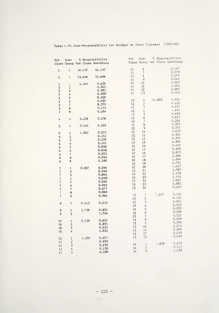
Table 1.39. Cost-Responslblllty for Bridges on State Highways (1985-86)
Veh Sub- X Responsibility
Class Group Veh Class Sub-Group
9 1
9 2
10 1
10 2
10 3
10 4
11 1
11 2
11 3
11 4
11 5
16.137
5 5.606
4.344
0.236
0.545
1.051
0.507
0.213
1.7 39
0.126
1.350
16.137
5 5.606
0.6260.3450.9010.6900.4500.6070.3700.1710.184
0.236
0.545
0.275
0.1610.124
0.1110.0400.0480.0530.0540.185
0.0560.0400.0440.0500.0460.0610.0750.0690.066
0.213
0.0331.706
0.0310.0310.0330.031
0.0770.1020.2340.1300.109
Veh Sub- X Responsibility
Class Grou: Veh. Class Sub-Croup
0.1970.0780.0760.0620.0600.0630.0600.103
11 6
11 7
11 8
11 9
11 10
11 11
11 12
11 13
12 1
12 2
12 3
12 4
12 5
12 6
12 7
12 8
12 9
12 10
12 11
12 12
12 13
12 14
12 15
12 16
12 17
12 18
12 19
12 20
12 21
12 22
12 23
12 24
12 25
12 26
13 1
13 2
13 3
13 4
13 5
13 6
13 7
13 8
13 9
13 10
13 11
13 12
13 13
14 1
14 2
14 3
15.895
-.447
.828
0.0310.1200.457
1 .444
0.6950.6420.2860.3550.5550.5190.3310.3320.3940.4160.4000.5720.5841.0660.7011.0271.7871.3181.416
0.2670.081-.'."'
0.1050.1050.0610.0400.0300.0090.0200.0090.0090.014: . : :
-
0.0180.018
0.0780.3121.438
>22 -

Table 1.40. Cos t-Responslbl 11 ty for Bridges on County Roads (1985-86)
Veh Sub- Z Responsibility
Class Group Veh Class Sub-Croup
Veh Sub- I responsibility
Class Group Veh Class Sub-Croup
6 2
6 3
6 4
6 5
6 6
6 7
6 8
6 9
7 1
7 2
7 3
7 4
7 5
7 6
7 7
7 8
7 9
9 1
9 2
10 1
10 2
10 3
10 4
11 1
11 2
11 3
11 4
11 5
15.039
6 3.124
6.958
0.251
0.622
2.124
0.120
2.129
0.987
15.039
6 3.124
1 .206
0.4301.6180.9250.4781.2000.6710.1720.258
0.251
0.622
0.4550.3250.1520.1520.0710.0990.0990.1120.659
0.0100.0100.0100.0120.0090.0160.0160.0190.019
0.
2.129
0.
0.
0.
0.
0.0680.0680.1610.0810.046
11 6
11 7
11 8
11 9
11 10
11 11
11 12
11 13
12 1
12 2
12 3
12 k
12 5
12 6
12 7
12 8
12 9
12 10
12 11
12 12
12 13
12 14
12 15
12 16
12 17
12 18
12 19
12 20
12 21
12 22
12 23
12 24
12 25
12 26
13 1
13 2
13 3
13 4
13 5
13 6
13 7
13 8
13 9
13 10
13 11
13 12
13 13
14 1
14 2
14 3
4. = 14
0.937
182
056056
032032041
0.041
0.122
.
—
"
0.0080.0160.0490.3890.0860.1770.0160.0650.1810.1630.0460.0690.1160.0870.1010.0670.1320.4770.2590.4630.7550.4140.5770.0690.0160.016
0.2810.2810.1870.0940.093
0.
0.
0.0.
0.0.
0.
0.
0.1560.7541.988
- 223

Table L 41. Cos t-Responslblll ty for Bridges on City Streets (1985-86)
Veh Sub- 7. Responsibility
Class Group Veh Class Sub-Group
3 2
3 3
3 &
3 5
3 6
3 7
3 8
3 Q
23
&5
6
89
1
2
3
4
5
67
89
9 1
9 2
10 i
10 2
10 3
10 4
11 1
11 2
11 3
11 4
11 5
15.935
60.972
3.486
0.829
0.466
1.467
0.124
2.286
0.129
1.205
15.935
60.972
0.6660.2380.8810.5040.2140.5390.2780.0710.096
0.829
0.466
0.3740.2670.1180.1180.0480.0620.0620.0680.350
0.0120.0120.0120.0130.0100.0160.0160.0170.017
0.
0.
2. 286
032032032
032
.100
.100
.208
.104
.057
Veh Sub- Z Responsibility
CLass Group Veh Class Sub-Group
0.2250.0670.0670.0370.0370.0440.0440.116
11 6
11 7
11 8
11 9
11 10
11 11
11 12
11 13
12 1
12 2
12 3
12 4
12 5
12 6
12 7
12 8T 5 9
12 10
12 11
12 12
12 13
12 14
12 15
12 16
12 17
12 18
12 19
12 20
12 21
12 22
12 23
12 24
12 25
12 26
13 1
13 2
13 3
13 4
13 5
13 6
13 7
13 8
13 9
13 10
•3 11
13 12
13 13
14 1
14 2
14 3
1 1 . 507
0.363
1.420
0.0280.0570.1681.1800.2620.5160.0480.1900.5090.4560.1240.1860.2900.2180.2390.159
0.2941.064
0.544
0.9721.517
0.8321.3950.1670.0460.046
0.1090.1090.07 3
0.0360.036
0.
0.
0.0.
0.
0.0.
0.
0.0400.2041.176
- 224 -
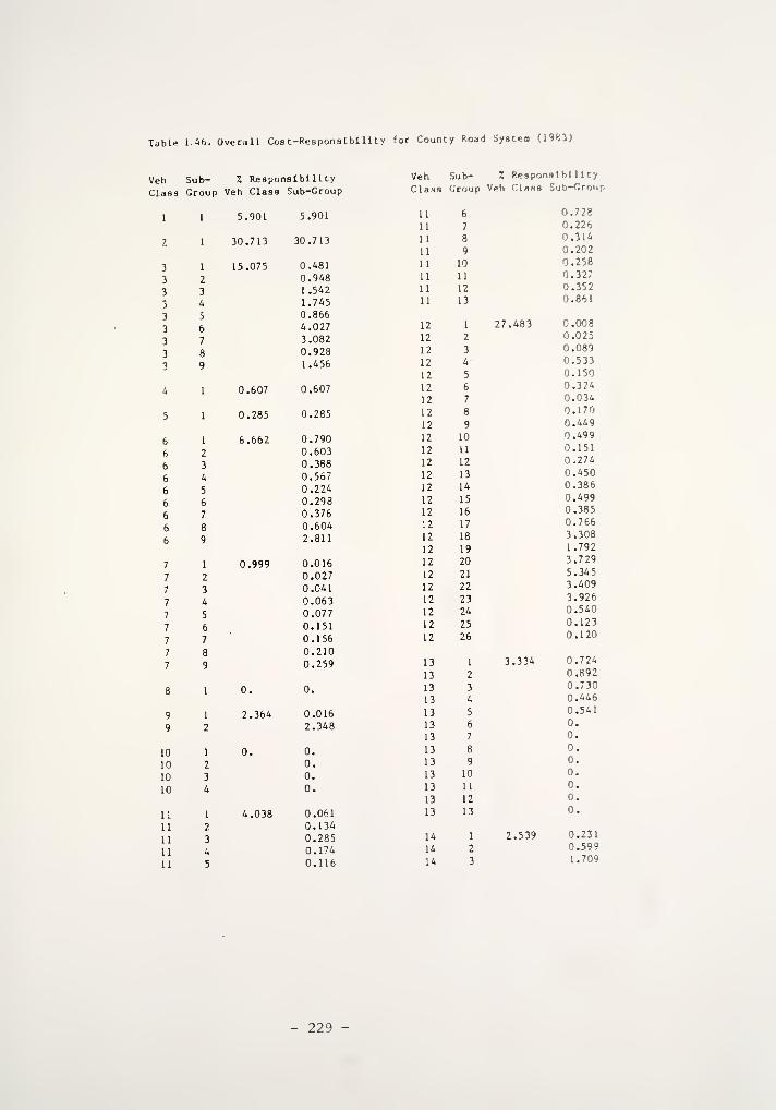
Table 1.4b. Overall Cost-Responslblllty for County Road System (1983)
Veh Sub- 7. Responsibility
Class Group Veh Class Sub-Croup
1 1 5.901 5.901
2 1 30.713 30.713
3 1 15.075 0.481
3 2 0.948
3 3 1.542
3 4 1.745
3 5 0.866
3 6 4.027
3 7 3.082
3 8 0.928
3 9 1.456
4 1 0.607 0.607
5 1 0.285 0.285
6 1 6.662 0.790
6 2 0.603
6 3 0.388
6 4 0.567
6 5 0.224
6 6 0.298
6 7 0.376
6 8 0.604
6 9 2.811
7 1 0.999 0.016
7 2 0.027
7 3 0.041
7 4 0.063
7 5 0.077
7 6 0.151
7 7 0.156
7 8 0.210
7 9 0.259
8 1 0. 0.
9 1 2.364 0.016
9 2 2.348
10 1 0. 0.
10 2 0.
10 3 0.
10 4 0.
11 1 4.038 0.061
11 2 0.134
11 3 0.285
11 4 0.174
11 5 0.116
Veh Sub- Z Responsibility
Class Group Veh Class Sub-Group
0.7230.2260.3140.2020.2580.3270.3520.861
11 6
11 7
11 8
11 9
11 10
11 11
11 12
11 13
12 1
12 2
12 3
12 4
12 5
12 6
12 7
12 8
12 9
12 10
12 11
12 12
12 13
12 14
12 15
12 16
12 17
12 18
12 19
12 20
12 21
12 22
12 23
12 24
12 25
12 26
13 1
13 2
13 3
13 4
13 5
13 6
13 7
13 8
13 9
13 10
13 11
13 12
13 13
14 1
14 2
14 3
27.483
3.334
2.539
0.0080.0250.0890.5330.1500.3240.0340.1700.4490.4990.1510.274
0.4500.3860.4990.3850.7663.308
1.7923.7295.3453.409
3.9260.5400.1230.120
0.7240.8920.7300.4460.5410.
0.
0.
0.
0.
0.
0.
0.
0.2310.5991.709
- 229 -

Table 1.47. Overall Cost-Responslbl llty for City Street Systea ( 1983J
Veh Sub- 7. Responsibility
Class Group Veh Class Sub-Group
Veh Sub- Z Responsibility
Class Group Veh Class Sub-Croup
1 1 10 .4 34 10.434
2 1 41 .798 41.798
3 1 3 .649 0.352
3 2 0.318
3 3 0.541
3 4 0.456
3 5 0.191
3 6 0.792
3 7 0.567
3 8 0.170
3 9 0.263
6 1
6 2
6 3
6 4
6 5
6 6
6 7
6 8
6 9
7 I
7 2
7 31 4
7 5
7 6
7 7
7 8
7 9
1.074
0.282
2.139
0.398
0.
1.074
0.282
0.3280.2460.1380.1880.068
0.0900.111
0.1700.801
0.0090.0140.0190.0270.0330.0590.0610.0800.097
0.
9 1 0.838 0.006
9 2 0.832
10 1 0.144 0.027
10 2 0.033
10 3 0.036
10 4 0.048
11 1 2.248 0.059
11 2 0.093
11 3 0.18511 4 0.110
11 5 0.070
11 6
11 7
11 8
11 9
11 10
11 11
1 1 12
11 13
12 1
12 2
12 3
12 4
12 5
12 6
12 7
12 8
12 9
12 10
12 11
12 12
12 13
12 14
12 15
12 16
12 17
12 18
12 19
12 20
12 21
12 22
12 23
12 24
12 25
12 26
13 1
13 2
13 3
13 4
13 5
13 6
13 7
13 8
13 9
13 10
13 11
13 12
13 13
14 1
14 2
14 3
36.011
0.617
:.
o.
o.
0.386
0.4150.1280.173
.. -
0.1370.1720.174
0.423
0.0170.0460.1540.875.233
.491
.051
0.2440.6410.6950.2090.3710.6080.514
0.6650.5060.9984.2902.3134.799
6.8864.37 5
5.0340.6910.1580.148
0.141" ..T ;
0.1340.0800.095
0.
0.
0.
0.
0.
0.
0.
0.
0.032
0.270
230 -

Table 1.48. Overall Cost-Responslblllty for State Highway System (1985-86)
Veh Sub- Z Responsibility
Class Group Veh Class Sub-Group
1 1 13 321 13.321
2 1 46 .179 46.179
3 1 3 .750 0.391
3 2 0.244
3 3 0.599
3 4 0.585
3 5 0.370
3 6 0.628
3 7 0.433
3 8 0.221
3 9 0.278
6 2
6 3
6 4
6 5
6 6
6 7
6 8
6 9
7 1
7 2
7 3
7 4
7 5
7 6
7 7
7 8
7 9
10 1
10 2
10 3
10 4
0.220
0.491
1.001
0.876
0.141
0.787
0.114
1.840
0.220
0.491
0.2040.1270.1060.1160.045
0.0470.0560.0690.230
0.0420.0390.0520.0710.0760.1150.1480.1570.175
0.141
027
760
.023
026.031
.034
.056
.093
.213
.120
.127
Veh Sub- Z Responsibility
Class Group Veh Class Sub-Croup
0.2360.1020.1150.1110.1280.1430.1510.244
11 6
li 7
11 8
11 9
11 10
11 11
11 12
11 13
12 1
12 2
12 3
12 4
12 5
12 6
12 7
12 8
12 9
12 10
12 11
12 12
12 13
12 14
12 15
12 16
12 17
12 18
12 19
12 20
12 21
12 22
12 23
12 24
12 25
12 26
13 1
13 2
13 3
13 4
13 5
13 6
13 7
13 8
13 9
13 10
13 11
13 12
13 13
14 1
14 2
14 3
29.836
0.744
0.707
0.0260.1150.4451.2800.7590.6370.3590.4 26
0.5710.5900.4250.4690.5500.6580.6941.057
1.1272.2061.6432.7464.5974.1183.1190.8630.1340.223
0.1000.1160.09 5
0.0720.0550.0260.0440.0200.0220.0380.0240.0600.073
0.0570.1420.5(19
- 231

Ta ble 1.49. Overall Cost-Responslbl llty for County Road System (1985-86)
Veh Sub- X Responsibility
Class Group Veh Class Sub-Group
7 2
7 3
7 4
7 5
7 6
7 7
7 8
7 9
9 1
9 2
10
10
1
2
10 3
10 4
11 1
11 2
11 3
11 4
11 5
6.412
32.501
13.836
0.4 38
0.299
6.211
0.999
2.543
0.
3.924
6.412
32.501
0.4950.2911.5381.6980.8343.835
2.941
0.8721.331
0.438
0.299
0.717
0. 580
0.,368
0..513
0.,213
0.,281
0..352
0,,570
2 .617
.017
.026
.041
.064
.070
.149
.154
.213
.265
0. 011
2. 531
0.
0.
0.
0,
0,.067
0.,145
0,.275
.162
.105
Veh Sub- % Responsibility
Class Croup Veh Class Sub-Croup
0.6590.2010.2820.1870.2390.3030.3770.925
11 6
11 7
11 8
11 9
11 10
11 11
11 12
11 13
12 1
12 2
12 3
12 4
12 5
12 6
12 7
12 8
12 9
12 10
12 11
12 12
12 13
12 14
12 15
12 16
12 17
12 18
12 19
12 20
12 21
12 22
12 23
12 24
12 25
12 26
13 1
13 2
13 3
13 4
13 5
13 6
13 7
13 8
13 9
13 10
13 11
13 12
13 13
14 1
14 2
14 3
27.004
3.224
2.610
0.0090.0240.0880.5200.1480.3140.0340.1660.4350.4890.1450.2670.4380.3990.4730.3730.7623.264
1.7703.6655.2353.3453.8590.5260.1200.136
0.6730.8520.7120.4420.544
0.
0.
0.
0.
0.
0.
0.
0.
0.2340.572
232 -

Table 1.50. Overall Cost-Responslblllty for City Street Syaten (1985-86,
Veh Sub- X Responsibility
Class Group Veh Class Sub-Croup
6 2
6 3
6 4
6 5
6 6
6 7
6 8
6 9
7 1
7 2
7 3
7 4
7 5
7 6
7 7
7 8
7 9
9 1
9 2
10 1
10 2
10 3
10 4
11 1
11 2
11 3
11 4
11 5
10.327
41.349
3.440
0.769
0.279
2.060
0.420
0.960
0.152
2.267
10.327
41.349
0.3400.1420.5400.4560.1900.7890.5670.1670.249
0.769
0.279
0.307
0.2410.1340.1750.0680.0870.108
0.1670.772
0.0100.0140.0200.0290.030
0.061
0.0630.0860.106
0.
0.0050.956
0.0260.0330.0390.054
0.0630.1030.1830.1050.065
Veh Sub- Z Responsibility
Cla98 Croup Veh Clasa Sub-Croup
0.3850.1160.1580.1030.1300.1630.2020.492
11 6
11 7
11 8
11 9
11 10
11 11
11 12
11 13
12 1
12 2
12 3
12 4
12 5
12 6
12 7
12 8
12 9
12 10
12 11
12 12
12 13
12 14
12 15
12 16
12 17
12 18
12 19
12 20
12 21
12 22
12 23
12 24
12 25
12 26
13 1
13 2
13 3
13 4
13 5
13 6
13 7
13 8
13 9
13 10
13 11
13 12
13 13
14 1
14 2
14 3
36.958
0.621
0.0190.0450.1560.8770.2360.4900.0520.2470.6410.7060.2060.3770.6130.5540.6520.5101.0404.4312.3934.939.042
.488
.192
.706
.162
.183
0.135166
136083101
0.411
0.
0.0.0.
0.
0.
0.
0.
;.::•-
0.083
- 233 -
APPENDIX J
PROBLEMS OF USING CENTS PER VEHICLE-MILES OF TRAVEL AS AN INDEX
FOR EXPRESSING COST-ALLOCATION RESULTS
The index cents/VMT was used in a number of cost-allocation studies to
asses whether individual vehicle types were paying their fair share of cost
responsibilities. This index is not adopted in this study to compare cost-
responsibilities of vehicle classes and their revenue contribution because of
a number of problems involved in its use.
Firstly, it is recognized that the index cents/VMT does not have a sound
meaning in cost-allocation analysis. This is because not all expenditure
items are functions of vehicle-miles of travel. For instance, a large portion
of bridge related costs cannot be meaningfully related to vehicle-miles of
travel. Consider two vehicle classes with identical percentage cost-
responsibility of bridge construction cost based on individual vehicular load-
ing consideration. When expressed in terras of cents/VMT, the vehicle class
with a higher VMT would have a lower cents/VMT value. This appears to suggest
that one vehicle class has a lower "unit cost' than the other, which is actu-
ally not true. This clearly indicates that cents/VMT Ls a poor unit cost-
responsibility measure in cost-allocation study where many expenditure items
could not be allocated in direct proportion to vehicle class VMT. One must
therefore be refrained from making comparison on the relative cost-
responsibility of vehicle classes based on their cents/VMT values.
Secondly, since all user revenues can not be related to vehicle-miles of
travel, the use of cents/VMT to measure vehicle class revenue contribution ls
a misrepresentation.
234 -

Lastly, the terra cents/VMT, as it is being used in cost-allocation, Is
not uniquely defined. There are a few possible ways of computing cents/VMT
cost-responsibility for vehicle classes in cost-allocation study, and eacl
produces a different set of cents/VMT values. A simple hypothetical example
is presented below to illustrate this point.
Consider a cost-allocation problem involving two highway classes and two
vehicle classes. The total expenditures on highway classes 1 and 2 are
$90,000 and $ 10,000 respectively, and the results of cost-allocation analysis
are summarized in Table J.l.
The results in Table J.l indicate that vehicle class A underpays by
$8,000 or 13.33%, and vehicle class B overpays by $8,000 or 20.00%. A fair
revenue collection scheme would require vehicle class A to increase its con-
tribution by 13.33%, and vehicle class B to decrease by 20.00%.
Table J. 2 shows four differents ways by which the same cost-allocation
results may be expressed in terms of cents/VMT. Method (a) produces the same
conclusion as that in Table J.l regarding cost-responsibility. However, the
resultant cents/VMT values are illogical and misleading in the sense that
vehicle class A is lower in cents/VMT value than vehicle class B for both
highway classes 1 and 2, yet the computed resultant cents/VMT values indicate
the opposite.
Methods (b), (c) and (d) compute weighted average values of cents/VM'
using different parameters as weighting factors. Method (b) concludes that
both vehicle classes A and B are overpaying, whereas method (c) indicates that
both are underpaying. The last method, method (d), leads to yet another con-
clusion: vehicle class A overpays and vehicle class B underpays.
- 235

Table J.l Cost-Allocsilon analysis of Example Problem
(a) Problem data
Highway Class 1 Total Expenditure
Total Mileage
Total VMT
$90,000
10,000 miles
10 x 106
Vehicle Class A VMT 8 x 10
Vehicle Class B VMT 2 x 10
Highway Class 2 - Total Expenditure $10,000
Total Mileage 20,000
Total VMT 10 x 10
Vehicle Class A VMT 5 X 10
Vehicle Class B VMT 5 x 10
Revenue Contribution - Vehicle Class A $60,000
Vehicle Class B $40,000
(b) Cost-Allocation Results
Highway Class 1 Highway Class 2 Total Cost- Total Revenue
Cost-Responsibility Ccst-Xesponsibility Responsibility Contribution
Vehicle Class A
Vehicle Class B
$64,000
$26,000
$4 , 000
36,000
$68,000
$32,000
$60,000
$40,000
- 236 -

The example above shows that, depending on the computational procedure
adopted, the final cost-responsibility values expressed in cents/VMT can vary
over a relatively wide range. Conclusions drawn from different versions of
cents/VMT values also can be very different. The problem of these conflict
results is further complicated by the fact that none of the four procedures
presented in Table J. 2 can be claimed to be perfect, and none can be sai<
be completely wrong.
Based on the discussion above, it is clear that a fair and sound coc-
parison between vehicle classes' cost-responsibilities and their revenue con-
tribution cannot be made by expressing cost-responsibilities or revenue con-
tribution or both in cents/VMT. It was therefore decided that the results of
the present study would not be expressed in terms of cents/VMT.
- 237 -

<3 S
I -. Ou Xi O
Sg
Sg
O —I M
< =3 O
it in Oa «n otz. n t*-
G u -j
- 238
REFERENCES
1. American Association of State Highway and Transportation Officials, A
Policy on Geometric Design of Highway and Streets ,1984 .
2. American Association of State Highway and Transportation Officials,
AASHTO Interim Guide for Design of Pavement Structures , 1981 .
3. American Association of State Highway and Transportation Officials, Stan-
dard Specifications for Highway Bridges , 12th edition, 1977.
4. Black, J. E. and J. G. Pigman, "Allocation of Transportation Costs to
Users," Kentucky Transportation Research Program, University of Kentucky,
May, 1982.
5. Census of Transportation U.S., "Summary: Truck Inventory and Use Survey",
1977.
6. Colucci-Rios B., and E. J. Yoder, "Effects of Raising Load Limits on
Pavements and Bridges in Indiana," JHRP-79-23, Purdue University, 1979.
7. Congressional Budget Office, "Guidelines for a Study of Highway Cost
Allocation," U.S. Congress, February, 1979.
8. Connecticut Department of Transportation, "Highway User Costs in Connec-
ticut," Office of Research, Report No. 8505 l-F-82-1 , February, 1982.
9. Federal Highway Administration, "Final Report on the Federal Highway Cost
Allocation Study," May, 1982.
10. Federal Highway Administration, Incremental Analysis of Structural Con-
struction Costs , Report FHWA/pl/8 1/008, April, 1981.
11. Florida Department of Transportation, "Florida Highway cost Allocation
Study," December, 1979.
12. Fwa, T. F. and K. C. Sinha, "Thickness Incremental Method for Allocating
Pavement Construction Costs in Highway Cost-Allocation Study," to be
presented at the 1985 Annual Meeting of Transportation Research Board,
Washington, D.C.
13. Fwa, T.F. and K.C. Sinha, "A Performance-Based Approach for Determining
Cost-Responsibilities of Load-Related and Non-Load-Related Factors in
Highway Pavement Rehabilitation and Maintenance Cost Allocation," to be
presented at the 1985 Annual Meeting of Transportation Research Board,
Washington, D.C.
14. Georgia Department of Transportation, " Georgia Highway Cost Allocation
Study," March, 1979.
15. Highway Research Board Special Report 61E, "The AASHTO Road Test, Report
5, Pavement Research," 1962.
- 239 -
16. Highway Research Board Special Report 87, Highway Capacity Manual, 1_965.
17. Huff, T.S. and F.H. Scrivner, "Simplified Climbing-Lane Design Theory and
Road'lest Results," Highway Res earch Board Bulletin 104_, 1955.
18. Indiana Department of Highways, Contract Proposals Section, Catolog o_f
LLP. A. Prices lor Roads , Bridges nnd Traffic ItcmH, 1983.
19. Indiana Department of Highways, Division of Mai ntenance .Field Operations
Handbook for Foremen 1982 - 1983 .
20. Indiana Transportation Coodinating Board, Indiana Transportation Fact
Book , June 1982.
21. Iowa Department of Transportation, "Final Report of the Iowa Highway Cost
Allocation Study," 1982.
22. Joint Legislative Audit and Review Commission, State of Virginia, "Vehi-
cle Cost Responsibility in Virginia," January, 1982.
23. Kent, P. M. and M. T. Robey, 1975-1979 National Truck Characteristic
Report, U.S. Department of Transportation, FHWA, June 1981.
24. Kiley, E.V., "Concept of Cost Functions and Incremental Solutions of
Vehicle-Tax Allocation Problem," HRB Bulletin 121 ,Highway Research
Board, 1956.
25. Lewis, D. and R. A. Barnhart, Road User and Property Taxes, On Selected
Motor Vehicles, U. S. Department of Transportation, FHWA, 1982.
26. MacTavish, Douglas and Neumann, Donald L. , Vehicle Classification Case
Study for_ the_ Highway Performance Monitoring System ,Federal Highway
Administration, August, 1982.
27. Maine Department of Transportation, "Final Report of the Maine Highway
Cost Allocation Study," December, 1982.
28. Maine Department of Transportation, "Main Highway Cost Allocation," Work-
ing Paper No. 3, 1982.
29. Mannering, Fred L. and K. C. Sinha, "Methodology for Evaluating Impacts
of Energy, National Economy, and Public Policies on Highway Financing and
Performance," Transportation Research Record 7j42, Transportation Research
Board, 1980, pp. 20-27.
30. Metwali, S., "Framework for a Pavement Evaluation System," JHRP-S1-7,
Purdue University, 1981.
31. Mohan, S., "Development of a System for the Evaluation of Pavements in
Indiana," Interim Report, JHRP-78-21, Purdue University, 1978.
32. North Carolina Department of Transportation, "North Carolina Highway Cost
Allocation Study," Final Report, March, 1983.
- 240

33. Oregon Department of Transportation, "1980 Motor Vehicle Cost Responsi-
bility Study," March, 1981.
34. Rauhut, J. B., R. L. Lytton and M. I. Darter "Pavement Damage Functions
for Cost Allocation: Vol. I. Damage Functions and Load Equipment Fac-
tors," FHWA, DOT FH61-80-C-00175, Draft Final Report, July, 1982.
35. Reno, Arlee, T. , B. J. Ritchey, and J. R. Morris, Transportation System
Descriptors Used in Forecasting Federal Highway Revenues, U.S. Department
of Transportation, FHWA, June 1981.
36. Sharaf, Essam A., K. C. Sinha and E. J. Yoder, "Energy Conservation and
Cost Saving Related to Highway routine Maintenance: Data Collection and
analysis of Fuel Consumption," JHRP-82-83, Interim Report, Joint Highway
Research Project, School of Civil Engineering, Purdue University,
December, 1982.
37. Sharaf, E. A. and K. C. Sinha, "Estimation of Pavement Routine Mainte-
nance Costs," Joint Highway Research Project, School of Civil Engineer-
ing, Purdue University, October, 1983.
38. Sinha, K.C. et al., "Indiana State Highway Reciprocity Study: Final
Report", JHRP-83-15, Joint Highway Research Project, School of Civil
Engineering, Purdue University, October, 1983.
39. Sinha, K.C. et al., "Indiana Highway Cos t-Allocaion Study: A Report on
Methodology", FHWA/IN/JHRP - 84/4, Joint Highway Research Project, March,
1984.
40. Taragin, A., "Effect of Length of Grade on Speed of Motor Vehicles,"
Highway Research Proceedings , 1945.
41. Transportation Development Associates, Inc., "Washington State Highway
Cost Allocation Study," January, 1977.
42. University of Maryland, "Maryland Cost Allocation Study," February, 1983.
43. U.S. Department of Transportation, FHWA, Highway Statistics , 1979, 1980,
1981, 1982.
44. U.S. Department of Transportation, FHWA, Highway Taxes and Fees , How Thev
are Collected and Distributed , 1982.
45. Wilbur Smith and Associates, "Highway User Fee Study," prepared for the
Joint Transportation and Highways Interim Committee, Wyoming State Leg-
islature, February, 1981.
46. Willey, W.E., "Uphill Speeds of Trucks on Maintenance Grades," Highway
Research Board Proceedings , 1949.
47. Winfrey, R. , Economic Analysis for Highways , International Textbook Com-
pany, 1968.
- 241 -

48. Wisconsin Department of Transportation, "Highway Cost Allocation Study,"Final Report, December, 1982.
49. Yoder, E.J. and M.W. Witczak, Principles of Pavemen t Design , 2nd Edition,John Wiley & Sons, 197 5.
50. Yoder, S. R., Chief, Division of Design, "Indiana Pavement Design Pro-cedure," Memo dated October 3, 1978, Revised November 3, 1983, IndianaDepartment of Highways.
- 242 -