1  

Indirect Pollution Haven Hypothesis in a context of Global Value Chain 

 

Arce González, Guadalupe; Cadarso Vecina, María‐Ángeles; López Santiago, Luis‐Antonio; Tobarra Gómez, María‐Ángeles; Zafrilla‐Rodríguez, Jorge 

 Universidad de Castilla‐La Mancha Facultad de Ciencias Económicas y Empresariales, 

Plaza de la Universidad n. 2, 02071, Albacete (Spain) 

Phone +34 967 599 200 Ext. 2383  

E‐mail: Guadalupe.Arce@alu.uclm.es, Angeles.Cadarso@uclm.es, 

Luis.LSantiago@uclm.es, MariaAngeles.Tobarra@uclm.es; Jorge.Zafrilla@uclm.es 

 

Firms  locate  different  stages  of  their  production  in  third  countries with  the  aim  of 

reducing costs (labour, institutional, raw materials, etc. and also environmental costs), 

increasing  their  flexibility  and,  finally,  generating  growing  economies  of  scale.  This 

international  fragmentation  of  production  has  led  to  a  big  increase  in  international 

trade  of  final  goods  and,  particularly,  intermediate  inputs.  This  paper  investigates 

whether there is a positive or negative link between value added provided by different 

countries to the global production chains and their environmental  impact. In order to 

do  this we  develop  a multi‐region  input‐output model  that  allows  us  to  isolate  the 

different rounds or stages of production required by a good to reach final demand, and 

in this way, to calculate emissions generated by this product in several countries. 

The impact on climate change from global value chains depends on three factors. First, 

technology used in the factory located in the emerging country. Second, differences in 

energy and environmental intensity that exist along the chain of suppliers between the 

countries  of  origin  and  destination.  Third,  increase  in  distance  and  international 

transport linked to the growth in international trade of these components (Cadarso et 

al., 2010). A negative relationship between total value added and total CO2 emissions 

linked  to  global  production  chains,  and  focused  on  emerging  countries, will  show  a 

disconnection between economic and environmental costs. Firms would not take into 

account indirect costs on environment when making decisions on location or on origin 

of their suppliers, as they do not internalise these costs. This would support an indirect 

pollution  haven  hypothesis,  as  the  fall  in  trade  barriers  would  have  implied  a 

transformation  of  global  production  chains  that,  together  with  a  growth  in  trade, 

would  have  boosted  global  emissions.  This  increase  would  not  be  due  to  using  a 

technique  that  is  directly  less  efficient  in  terms  of  emissions,  but  because  of  their 

linkage  effects  with  production  and  emissions  in  the  country  of 

production/origin/destination  and with  the  emissions  linked  to  international  freight 

transport.  

2  

1. Introduction 

International  freight  transport has  increased  from 5.5%  to 21% of worldwide GDP  in 

1950 in 2007 (WTO, 2008). A third of this international trade is due to the exchange of 

final goods, while the other two thirds are explained by trade  in  intermediate  inputs 

(Johnson  and Noguera, 2012). Offshoring processes  and  global  chains of production 

are responsible for such a growth in inputs trade. Firms in developed countries divide 

their production  in several stages and  locate them  in emerging countries where they 

benefit  from  a  comparative  advantage  (wages,  flexibility,  environmental  regulation, 

taxes, etc). 

Environmentally  the effect  is such  that 30% of emissions  linked  to production  in  the 

world  economy  in  2004  are  internationally  traded  (Davis  et  al.,  2011).  This  impact 

differs between developed and developing countries  (Wiedmann et al., 2007; Peters 

and Herwitch, 2008a; Chen and Chen, 2011; Davis et al., 2011). The methodology of 

emissions balance shows a deficit  for developed countries, as they  import directly or 

indirectly  CO2  intensive  goods  in  exchange  for  exporting  environmentally‐friendly 

goods, and they suffer trade deficits. Currently, it is possible for developed countries to 

overcome Kyoto Agreement by not producing domestically polluting goods, but buying 

them  from  foreign  countries  (Muradian  et  al.,  2002). On  the  other  hand,  Levinson 

(2009)  found  for US  international  trade  that  the  increase of net  imports of polluting 

goods accounts only for a small proportion of the pollution reductions in emissions by 

US  manufacturers.  Emerging  countries,  on  the  contrary,  present  a  surplus  in  the 

emissions balance as they, on the one hand, export goods more CO2 intensive than the 

ones  they  import,  and  on  the  other,  keep  trade  surplus  in  final  and,  above  all, 

intermediate  inputs commerce. Nevertheless, we cannot use this balance to quantify 

whether the impact from trade on the environment allows us to reduce emissions for 

the world as a whole. The  reason  for  this  is  that  the  trade balance  is different  from 

zero while  the  sum of  the emissions balance  for all  countries  in  the world  is always 

zero. 

From the point of view of the global economy, it is most efficient to produce each good 

where  it  pollutes  the  least, where  there  is  a  comparative  environmental  advantage 

(Peters  and  Herwitch,  2008a),  both  direct  and  indirectly.  The  Pollution  haven 

hypothesis  (PHH)  implies  that  a  reduction  in  trade  barriers  increases  trade  and 

subsequently  emissions  (Coopeland  and  Taylor,  2004).  This  hypothesis  is  analysed 

using  the  balance  of  avoided  emissions  (BAE),  that  is  calculated  as  the  difference 

between emissions linked to exports and emissions avoided by imports in international 

trade. Mongelli et al. (2006) shows, using a single region input‐output model for Italy, 

the presence of carbon leakage, but they do not found support for the pollution haven 

hypothesis. Dietzenbacher and Mukhopadhyay (2007) and Zhang (2012) apply a single 

region input‐output model to the analysis of pollution embodied in exports, in terms of 

3  

emissions, and  that avoided by  imports,  for  India  in  the  first paper and China  in  the 

second.  Both  papers  find  a  negative  balance  in  net  exported  embodied  carbon,  for 

India  between  1991/992  and  1996/1997,  and  for  China  between  2000  and  2005. 

According  to  the  authors  this  result  shows  that  the  emissions  pattern  implies  that 

trade helped in both countries to lower its total carbon emissions. However, between 

2005 and 2007 emissions embodied in Chinese exports are higher than those avoided 

by imports, as the country becomes a net exporter. In terms of D&H this conforms to 

the PHH, as emissions grow via  international  trade  (even  though, according  to  these 

authors, we will also need to study the result of the emissions from this trade  in the 

rest of the world). 

Although  trade  means  a  country  can  avoid  emissions,  international  trade  might 

generate an  increase  in emissions for the world economy as a whole. Firstly, because 

we must realise that this trade might increase or decrease emissions in the rest of the 

world  (Dietzenbacher and Mukhopadhyay, 2007)1. Secondly, because a  single  region 

input‐output model does not take into account the successive rounds of international 

production. These problems are solved  in Chen and Chen (2011) as they use a multi‐

region input‐output (MRIO) model and calculate the difference between the emissions 

avoided by  imports (EAI) and emissions embodied  in  imports (EEI)2 between G7, BRIC 

and  the  rest of  the world  (ROW)  to evaluate  this effect. They  find  that world  trade 

increased emissions by 0.13 billion tons in 2004 over a total of 5.77 billion tons of EEI. 

Thirdly, it does not include the increase in emissions linked to the international freight 

transport of products that move around the globe as parts and components until they 

are finally assembled in final goods (Cadarso et al, 2010, Cristea et al. 2011). 

In this paper we develop a two‐region input‐output model and a multi‐region model to 

analyse whether  the  different  rounds  or  stages  of  production  and/or  trade  in  final 

goods are responsible for the existence (or not) of the PHH. Our proposal allows us to 

decompose  the BAE, by  countries and by  type of  traded goods,  into  three different 

balances: a) balance of avoided emissions in final goods, b) BAE in intermediate inputs 

required  for the  last stage of production, and c) BAE of  intermediate  inputs required 

for all other stages of production, from the first to the penultimate. This means we can 

isolate the role of the different countries  involved  in global chains of production and, 

from  that  point, we  can  analyse  their  environmental  impact.  Finally we  apply  this 

                                                            1 Dietzenbacher & Mukhopadhyay (2007) use a similar analysis by calculating the balance from a million euros of exports and avoided  imports, keeping constant  their  relative  industry distribution. A positive balance  would  imply  that  international  trade  generates  a  growth  in  emissions.  Nevertheless,  this measure  does  not  allow  us  to  isolate  the  importance  of  changes  in  industry  distribution  on  trade balance. 2 This means that Chen and Chen (2011) take into account simultaneously the technology of production in all considered countries, while  in  the papers by Dietzenbacher & Mukhopadhyay  (2007) and Zhang (2012) only technology for the country of analysis is included. 

4  

methodology  to  a  bi‐region model  of  trade  between  Spain  and China  in  the  period 

2000‐2010. 

The  paper  is  divided  in  four  sections.  Section  2  develops  the methodology  on  the 

impact of international trade on environment, and section 3 shows and comments the 

results  from  applying  this methodology.  Finally,  section  4  is  devoted  to  discuss  the 

main conclusions found in the paper. 

2. METHODOLOGY  

2.1 Trade balance in uni‐regional and bi‐regional models. 

The  expression  for  trade  balance  by  commodities  for  country  1  in  an  uni‐regional 

input‐output model is: 

1 1 1 1 1 1 11

1 1           (1) 

where   is country 1 exports vector,   is the domestic technical coefficient matrix, , 

 the imported coefficient matrix,   the final domestic demand vector and   the 

imported  final demand vector. A positive  sign  in a given  commodity  in  the  resulting 

vector points  to a surplus  in  the  trade balance  for  that commodity, while a negative 

sign points to a deficit. The aggregation of the vector elements is the trade balance for 

country 1. 

A bi‐regional model, works with information of country 1 and the rest of the world or 

country 2 ( ). With only two countries country 1 exports are equal to country 2 

imports, so the expression for trade balance for country 1would be the following (just 

the opposite for country 2): 

1 1 1 2 1 21

2 2 1 1 11

1 1     (2) 

where elements are similar to those  in expression 1 and suffix 2  indicates country 2. 

The use of    indicates diagonalised  vectors,  allowing  to work either by  rows or by 

columns. 

Expression 2 is modified by considering separately two demand ( ) components, the 

one that remain within frontiers, ( ), that contains private consumption,  investment 

and public expenditure, and exports  ( ). We also define  the  imports multipliers  for 

country 1 and 2,  . We then obtain three separate trade balances: 

1 2 1

3.1

2 2 1 1

3.2

2 2 1 1

3.3

    (3) 

Expression  3.1  quantifies  trade  balance  for  final  goods,  and  it measures,  for  each 

sector, the value of commodities sold to country 2 final consumers by country 1 (that 

might  be  private  or  public  consumption  or  investment  goods) minus  the  value  of 

5  

commodities  from country 2 by country 1  final consumers. Results are symmetric by 

rows or columns: millions of Euros per internationally traded commodity.  

Expression 3.2 quantifies trade of imported intermediate goods that will be used in the 

production  process  of  domestically  demanded  goods.  According  to  global  value 

changes  analysis,  these  goods  belong  to  the  last  commodities  international  trade 

round. Expression 3.2 provides different  lectures by rows and by columns. By rows  it 

calculates the difference between commodity i imports needed by country 1 (country 

2  exports)  and  those  needed  by  country  2  (country  1  exports)  to  produce  any 

commodity  consumed domestically. A positive  sign points  to  country 1  selling more 

intermediate commodity i, for country 2 domestically consumed production, than the 

purchased  one  for  domestic  production.  The  rows,  or  products,  result  shows  total 

exports and imports of commodity i between both countries. By columns, it shows the 

difference between exports and  imports of all the goods required to produce a given 

commodity  j  in  country  2  and  country  1,  but  only  for  that  part  of  j  that  is  sold 

domestically.  Therefore,  by  columns  we  obtain  international  dependence  of  a 

domestic  sector: a  strong negative  the  result  shows a high dependence of domestic 

final  demand  of  a  foreign  intermediate  good.  It  is  a  vertically  integrated  sectors 

analysis that does not measure direct trade for given commodities. 

Expression 3.3 shows trade balance for inputs that will be used in future international 

rounds of production, apart  from  the  last one collected by 3.2. Each element  in  this 

balance  accounts  for  the  value  of  global  value  chains  of  production.  Previous 

specialised  literature  defines  this  element  as  vertical  specialization  (Hummels  et  al 

2001),  so  that  signs  in  3.3  provide  information  on  differences  in  countries  vertical 

specialization  (Cadarso  et  al.  2007).  The  sign  of  this  element  shows  the  difference 

between  country  1  exports  that will  be  later  imported  as  part  of  final  goods,  and 

country 1 imports that will be exported embodied in final goods. A positive sign shows 

that country 1 is specialised in the production of goods that will have their last stage of 

production  in  other  countries  and will  be  re‐imported  as  final  goods, more  than  in 

importing intermediate goods that will be used to produce final goods.  

Analysing  by  components,  the  first  one  in  3.3  shows  intermediate  exports  from 

country 1 to country 2 required to produce final or  intermediate goods to country 1, 

and the opposite for the second component. We could think in GPS exports of country 

1 that country 2 fits in cars that will be sold to country 1. In a three goods example the 

relationships  are more  complex,  country  2  buys  country  1  chips  that  are  used  to 

produce GPS that will be sold to country 1 to be fitted in cars finally sold to country 2.  

In our example, working  in rows or commodities, country 1 exports are the result of 

the  aggregation  of  the  value  of  two  goods  (chips  and  cars  electronic  panel 

components) and  imports consider the value of one product, GPS. Therefore,  for the 

balance as a whole, exports are compensated in part by imports, however, analysis by 

6  

product will show surplus in chips and cars electronic panels for country 1  and deficit 

for GPS (the opposite for country 2). Sectoral unbalance could be unappreciable when 

working at an aggregate level. 

When working  by  columns,  results  show  imports  of  any  good  required  to  produce 

good j in country 1 that will be exported in its final stage to country 2  (the opposite for 

country  2).  As  it  happens  in  expression  3.2,  its  value  does  not  coincide  with  the 

commodities trade balance for both countries. 

2.2  Domestic emissions balance in uni‐regional and bi‐regional models. 

When building  a bi‐regional model balance of domestic emissions  (BDE), only  those 

emissions associated to the generation of value added that is responsibility of each of 

the  two  countries  are  considered,  but  leaving  aside  all  emissions  generated  in  any 

other stage of production or trade rounds. BDE  is useful to  isolate the environmental 

impact of trade between a country and the rest of the world  (SRIO) or between two 

countries or  geographical  areas  (bi‐regional).  This model  is  adequate  to  identify  the 

impact of delocalisation of  a  given  stage of production of  a  commodity  for  the  two 

implied countries, removing the effects in any other country. 

The calculation of a BDE for a uni‐regional model, (UBDE), is similar to the calculation 

of a  trade balance but considering  the domestic emission multipliers  for  the  implied 

country:  

1 1 1 1 1 2 1 1 11

1 1

       (4) 

where    is the domestic emissions multiplier for country 1, calculated by multiplying 

the emissions direct coefficient for country 1 ( ), or emissions per produced 

unit,  times  the  Leontief  inverse  ( ).  The  emissions  multiplier 

considers direct and  indirect emissions associated to the production of a unit of final 

product.  In a similar  fashion, country 2 domestic emissions multiplier  is calculated as 

.  It  is  also  possible  to  define  the  total  emissions multiplier,  that 

considers  all  emissions,  domestic  and  imported,  required  for  production  within  a 

country (  for country 2), what involve to work with Leontief inverse 

in total terms (domestic plus  imported technical coefficients). It  is  important to recall 

that  the  use  of  the  total  coefficients matrix  in  uni‐regional  and  bi‐regional models 

imposes  the  hypothesis  of  a  production  and  emissions  technology  similar  to  the 

domestic one for all the trading countries (domestic technology assumption, DTA). 

The expression for the domestic emissions balance in a bi‐regional model is similar to 

that in 3 multiplied by the country’s emissions multiplier: 

7  

1 1   1 1 2 2 2

5.1

2 1 1 1

5.2

      (5) 

Expression  (5)  provides  an  emission  balance  similar  to  the  definition  of  emissions 

embodied  in  bilateral  trade  (EEBT)  in  Peters  (2008).  Both  use  bilateral  trade  and 

domestic emissions  for each country production and sales, excluding the use of DTA. 

Also, neither takes  into account  international feedback emissions (Su and Ang, 2011). 

The main difference between them is that EEBT does not split the bilateral trade flow 

into  its  components,  intermediate and  final  consumption, whereas BBED does. As  a 

result,  they  imply  two different emission allocation criteria by  sector. EEBT allocates 

emissions  to  the origin sector,  the producing one. BBDE shows  the same  results and 

allocation criteria when considered by  rows. By columns, BBDE allocate emissions  to 

the user sector3 and shows different results. 

Within  the  domestic  emissions  balance  it  is  possible  to  consider  three  different 

elements, as it was the case for the trade balance: 

1 1   1 1 2 2 1

6.1

1 2 2 2 1 1

6.2

1 2 2 2 1 1

6.3

  (6) So  it  is possible  to distinguish  three  sub‐balances: 6.1 accounts  for  final goods  trade 

emissions; 6.2 for inputs trade emissions whenever inputs are in the last international 

production round, since they will be incorporated to final goods sold domestically; and, 

finally,  6.3  for  emissions  associated  to  any  previous  international  trade  rounds 

required to produce traded  intermediate  inputs that will keep on adding value  in the 

global value chain. 

The bi‐regional model can be used to isolate trade of country 1 with another country, 

country 2, or the rest of the world. For the two countries case, the impact on the rest 

of  the world  should also be  considered. As an example,  the amount of emissions  in 

goods produced by country 1 that will be used as intermediate inputs to produce final 

goods that will be exported elsewhere must be quantified. 

The distinction can be done by decomposing each country 1 y exported final demand 

as:  ,  where  the  first  element  accounts  for  country’s  2  exports  to 

country and the second country’s 2 exports to the rest of the world (the expression for 

country 1  is  ). As a  result, expression  in 6.3  can be decomposed  in 

two  expressions,  6.3.i  accounts  for  emissions  associated  to  consecutive  rounds  of 

production between country 1 and 2, while 6.3.ii. accounts for international rounds of 

commodities exchanged between countries 1 and 2 that end up as final goods to other 

                                                            3 As in a MRIO model. 

8  

countries (either as final or  intermediate goods). So expression  in 6  is transformed as 

follows: 

1 2 2 2 1 1

6.3

1 2 21 2 1 12

6.3.

1 2 2 2 1 1

6.3.

        (6.b) 

A temporal analysis of the previous balances provides  information on the  importance 

of  the  different  types  of  commodity  trade  on  environment. Our main  interest  is  to 

quantify the effect of global value changes on total emissions. It is also of great interest 

to develop both commodities/rows and sectors/ columns analysis, as commented for 

trade  balance  in  the  previous  section.  Finally,  the  minimisation  of  environmental 

effects can be studied by considering  the possibility of modifying emissions  intensity 

for specific countries. The possibility of technologies transference can be modelled and 

its consequences measured by the consideration of exchanging technical and polluting 

coefficient among countries.   

When only direct emissions are considered the expression becomes: 

1 1 1 1 2 2 1

6..1

1 2 2 1

6..2

1 2 2 1

6..3

 

   (6.c) 

In this case, 6.1, 6.2 and 6.3 show balances of avoided direct emissions associated to 

final  goods  trade,  last  round  intermediate  goods  and  inputs  in  other  production 

rounds. Differences between BBDE and dBBDE for each component measure the value 

of indirect emissions associated to international trade by commodities. 

2.3  Trade  and domestic  emissions balances  in  a multiregional  input‐output model 

(MRIO) 

The MRIO model widens  the basic  input‐output model  to  include  several  regions or 

countries  with  different  technology  and  trade  between  them.  For  the  sake  of 

simplicity, we consider two countries (r=2), denoted by superscript 1 and 2 (country 2 

is  the rest of  the world) and n sectors  (in subscripts).  In  this way, Aii  is  the matrix of 

domestic  production  coefficients  and Aij  is  the matrix  of  imported  coefficients  from 

country  i to country  j, yii  is the domestic final consumptions and yij  is country  i’s final 

demand exports to country  j. F  ij  includes all the emissions from country  i required to 

satisfy country j’s demand. Using the partitioned form to represent the model: 

 

12212122

12112112

22221121

22121111

21

12

2221

1211

22

11

2221

1211

2221

1211

0

0

0

0

yPyP

yPyP

yPyP

yPyP

y

y

PP

PP

y

y

PP

PP

FF

FF

    (7) 

9  

The first matrix shows emissions embodied in domestic final demand supplied by their 

own.  In  this matrix we have, by  rows, emissions  in one country  (first  row country 1) 

generated in the production of self‐covered domestic final demand of all countries. By 

columns, we have,  emissions  all over  the world  generated by  the  supplying of own 

final demand in one country (first column own final demand of country 1). The second 

matrix  in equation  (7) shows emissions embodied  in exports: by rows, emissions  in a 

country (first row country 1) embodied  in exports of both countries and, by columns, 

emissions  all over  the world embodied  in  a  country exports  (first  column  country 2 

exports).  

In a similar fashion as in the two‐region model, we can define the balance of domestic 

emissions  in  a multi‐region model  (BDEM)  for  country  1  as  the  difference  between 

domestic emissions linked to exports from country 1 (8.1) and emissions generated in 

the rest of countries from where all imports by country 1 come (8.2). The expression is 

as follows: 

1 1 1

11 12 12 22 12 21

8.1

21 12 21 11 22 21

8.211 12 22 21

8.3

12 22 21 11

8.4

12 21 21 12

8.5

 

                      (8) 

The  term 8.3 shows  the balance of emissions  linked  to  trade  in  final goods  (it  is  the 

same  as  6.1).  The  term  8.4  shows  the  balance  of  emissions  linked  to  trade  in 

intermediate inputs that belong to the last stage of international production, as when 

they enter the country these inputs become embodied in the production of final goods 

that  are  sold  domestically  (it  is  the  same  as  6.2).  Expression  8.5  is  the  balance  of 

emissions  linked  to any other  round of  international production  required  to produce 

final goods. This is the case as they are emissions of country 1 that enter country 2 and 

are used to produce in this country and later on exported (the opposite will be true for 

imports)  (it  is  the  same  as  6.3).  This  balance  captures  emissions  embodied  in  the 

consecutive  rounds  and  steps  of  the  production  of  a  commodity  caused  by  the 

fragmentation of production and the creation of global product chains.  

This  balance  of  domestic  emissions  has  some  advantages  versus  the  balances 

previously used in the literature. In comparison to the definitions of the emission trade 

balance (ETB) or the responsibility emission balance (REB) either used by Munksgaard 

and Pedersen (2001), Muradian et al. (2001), Peters and Hertwich (2008a), Ahmad and 

Wyckoff  (2003),  Sánchez‐Chóliz  and  Duarte  (2004)  and  Serrano  and  Dietzenbacher 

(2010),  there  is  no  cancelation  of  emissions  linked  to  the  imports  that  are  later 

exported in the BEDB and BDEM. This is a relevant component of trade and emissions 

that must not be neglected  in the measurement of environmental  impact of trade.  It 

10  

shows the international stages of production and would be considered as the emission 

equivalent to the concept of vertical specialization defined by Hummels et al. (2001). 

As opposed to the sales balance (SEB) of Kanemoto et al. (2012), where  international 

stages  of  production  do  not  cancel  out,  BEDB  and  BDEM  do  take  into  account 

emissions  linked  to  intermediate  inputs  that  are  not  included  in  SEB. On  the  other 

hand,  in  Kanemoto  emissions  balance  it  is  required  that  the  aggregation  of  all 

countries  balance  has  to  cancel  out  emissions,  as  it  happens  to  BEDB  and  BDEM. 

However, this property prevents the use of the balance to analyse whether the impact 

of trade on environment leads to a reduction in emissions. 

2.4 Pollution haven hypothesis in a context the global value chain 

Dietzenbacher & Mukhopadhyay  (2007), Zhang  (2011) and Chen & Chen  (2011)4 use 

the difference between emissions  linked  to exports  (EEX)  and emissions  avoided by 

imports  (EAM)  to  evaluate  whether  international  trade  increases  or  decreases 

emissions at a global level. If the first option can be proven, then we will be in the case 

called by D&H pollution haven hypothesis. Starting from the work of those authors and 

the  previous  decomposition  of  the  balance  of  domestic  emissions,  we  propose  a 

methodology  that  allows  us  to  analyse  whether  the  specialisation  of  countries  in 

different  stages of production and/or  trade  in  final goods generate an  increase or a 

decrease of emissions due to international trade. 

The  expression  that  calculates  the  impact of  trade on  the  growth of  emissions  in  a 

multi‐region model through the balance of avoided emissions (BAE) is as follows: 

EEX EAM εjXj

n

j 1

εjMi

n

j i

 

      (9) 

The  difference  of  this  balance  of  emissions  can  only  be  explained  by  the  different 

pollution  intensity of  the  trading countries, as exports  from one country are  imports 

for the rest ( ). This implies that a positive balance of BAE will conform to 

the  pollution  haven  hypothesis,  as  the  growth  in  emissions would  be  explained  by 

trade moving production to more polluting countries. The reason  is that,  in this case, 

emissions generated by trade are higher than if those goods had been produced within 

the  country  using  domestic  technology  and without  international  trade.  A  negative 

balance  for  the  BAE  implies  that  emissions  are  decreasing  due  to  trade  between 

countries,  as  goods  are  produced  where  they  generate  the  least  pollution. 

Nevertheless, this  formulation by D&H underestimates the  impact  from trade on the 

environment because: a)  it does  include  international freight transport, b)  it does not 

consider the possibility of global chains of production being different in both countries,                                                             4 Chen and Chen (2011) define it as emissions linked to imports and emissions avoided by those imports, even thought the result is not the same.

11  

meaning  that  the  country  where  imports  originate  might  also  move  part  of  its 

production  to other  country.  In order  to  solve  this  second problem we must  either 

build  a multi‐regional model  including  the whole world  economy  (Chen  and  Chen, 

2011)  or  a  two‐region model  that  considers  all  stages  under  the  DTA  assumption, 

changing  the  direct  ( )  by  the  total  emissions multipliers  ( ). However  emissions 

from international freight transport must be explicitly calculated (Cadarso et al., 2010). 

Our contribution is to decompose the balance of the BAE to analyse the importance of 

trade  in  different  types  of  goods,  intermediate  or  final,  for  the  environment  and 

therefore,  global  chains  of  production.  In  a  two‐region  (countries)  model,  the 

expression  that  reflects  emissions  from  exports  by  both  countries  is  (EEX): 

. Emissions avoided by those  imports are given by  (EEM):  . 

From that we propose to decompose the balance between them as: 

BAE ε1X1 ε2X2 ε1M1 ε2M2 ε1 M2 M1 ε2 M1 M2

1 2 2 2 2 1 1 1

2 2 2 2 1 1 1 1

1 2 1 1

10.1

2 1 2 2

10.1

1 2 2 1 1 1 2 1 1 2 2 2

10.2

1 2 2 1 1 1 2 1 2 2 2 1

10.3

 

                      (10) 

Expressions  10.1  show  the  balance  of  emissions  avoided  by  trade  in  final  goods 

between both countries. The terms in 10.2 show the balance of emissions avoided by 

trade in inputs that belong to the last stage of international production, as when they 

enter the country these inputs become embodied in the production of final goods that 

are sold domestically (it is the same as 6.2). Expression 10.3 is the balance of emissions 

linked to the rest of rounds of  international production required to produce goods to 

attend  final demand.  This  is  the  case  as  they  are emissions of  country 1  that enter 

country 2 and are used to produce in this country and later on exported (the opposite 

will be true for imports) (it is the same as 6.3). 

If we were to consider only direct emissions linked to international trade, the formula 

to calculate the balance of direct avoided emissions (BAEd) will be as follows: 

12  

e1X1 e2X2 eM1 e2M2

1 2 1 1

10..1

2 1 2 2

10..1

1 2 1 1 2 1 2 2

10...2

1 2 1 1 2 2 2 1

10..3

 

                      (10.b) 

Expressions 10..1, 10..2 and 10..3 show the balance of direct avoided emissions linked 

to trade in final goods, intermediate inputs for the final stage and inputs for the rest of 

stages of production. The difference between each component of BAE and BAEd would 

give us the indirect avoided emissions linked to international trade for each good. 

This same analysis can be implemented in a multi‐regional model, with the objective of 

identifying  the  importance  in  terms  of  environmental  impact  of  different  countries 

according  to  their  role  in  the  global  chains  of  production  and  of  different  types  of 

traded goods, intermediate and final. 

EEX EAM εjXj

2

j 1

εjMj

2

j i

11 12 12 22 12 21

11.

  21 12 21 11 22 21

11.

22 21 21 11 21 21

11.

  12 12 21 22 22 12

11.

11 12 11 21

11.1

22 21 22 12

  12 22 12 11 21 11 21 22

11.2

21 21 12 12

11.3

21 12 21 21

11.

 

                      (11) 

The meaning of expressions 11.1, 11.2 and 11.3 are similar  to expressions 10.1, 10.2 

and  10.3.  The  difference  is  that  the  first  ones  come  from  the MRIO  framework,  so 

these balances capture emissions embodied in the consecutive rounds and steps of the 

production  of  a  commodity  caused  by  the  fragmentation  of  production  and  the 

creation of global product chains.  

 

13  

3. Empirical application for Spanish‐Chinese trade 

3.1. Data sources 

Data  sources  for  the  paper  are  the  following:  OECD  2005  input‐output  tables,  in 

millions  of  Euros,  are  used  to  calculate  emissions  related  to  exports  from  Spain  to 

China;  Atmospheric  Emissions  Satellite  Accounts,  published  by  INE,  provide 

information on CO2 emissions in thousands of tons for the same year. Data have been 

aggregated to 28 sectors. Since Spanish input‐output tables do not provide information 

about  imports and exports by destination country, we have completed them by using 

Dirección  General  de  Aduanas  information  (Customs  Department)  to  obtain  the 

Spanish‐Chinese  trade  for  2005  and  2010.  Following  this  procedure  we  obtain 

emissions related to both countries for this period, to obtain these figures we suppose 

that, for the whole period, production and polluting technology remain constant as in 

2005. 

The calculation of  imports emissions has also been done working with OECD Chinese 

input‐output  tables, which  provide  data  expressed  in  10.000  Yuanes  (Renminbi),  so 

that the European Central Bank exchange rate was required to obtain results in Euros. 

Results  were  aggregated  to  23  sectors.  To  calculate  the  CO2  emissions  related  to 

energy goods consumption  IPCC  information on Carbon and CO2 emissions was used, 

as  well  as  data  on  Chinese  energy  consumption  for  2005  by  productive  sectors, 

provided by the China Statistical Yearbook annually presented by the National Bureau 

of Statistics of China. 

Chinese  emission  factors  have  been  obtained  based  on  IPCC  data5  on  emissions 

derived  from  energy  goods  combustion.  The  method  used,  explained  in  detail  in 

Annexe 2, is to multiply by the caloric conversion in carbon factor for each considered 

energy  source.  Following  this  procedure we  obtain  carbon  tons  by  product  took  to 

combustion. When  this  amount  is multiplied  by  the  oxidation  factor,  the  emissions 

factor  (tCO2/kt)  that  we  were  looking  for  is  obtained.  CO2  tons  (tCO2  from  now 

onwards) generated by the Chinese economy in 2005 will be calculated multiplying our 

emissions  factor  by  the  available Chinese  energy  consumption matrix  for  2005  (see 

annexe 2). 

Data on  imports by sector for Spain and China have been obtained from the Customs 

Department  in millions Euros. For each sector, two types have been considered, final 

goods  and  intermediate  goods,  by  using  the  proportion  of  those  for  total  industry 

imports. For international trade data the effect of prices has been deleted, taking into 

                                                            5 As noted in Zhang (2012), there exist different data sources to calculate emissions factors. We can find works like those of Peters et al. (2007), Zhang (2012) or Lin and Sun (2010) that, just like ours, combine data on energy consumption  from China Statistical Yearbook with  IPCC data on emission coefficients. Other papers like Liu et al. (2010) use data provided by the Chinese Energy Statistical Yearbook and the China Energy Data Book.

14  

account as reference year 2005. The GDP deflator given by the Bank of Spain has been 

used for Spanish data, while for Chinese data the GDP provided by the World Bank was 

used. 

3.2 Spanish‐Chinese trade: final and intermediate inputs 

The commercial relationships of Spain with the rest of the World have grown notably 

in  the  last  decades.  Only  the  2008  economic  crisis  curbed  temporarily  this  trend 

leading  to  a  reduction  in  economic  activity,  in  demand  and  a  lack  in  finance.  The 

original  increase  in  international  trade  was  explained  by  the  European  integration 

process, which was reinforced by an  increase  in worldwide trade relationships due to 

globalization and the entrance of China and India in the international scene.  

The  commercial  balance  between  Spain  and  China  is markedly  negative  for  Spain 

(Figure 2). While Spanish exports to China have kept at  low  levels, Chinese exports to 

Spain have been constantly increasing. Commercial deficit grows from 4.159 millions of 

Euros in 2000 to more than 14.880 in 2010. We must consider whether Spanish trade 

with  China  is  based  on  final  or  intermediate  goods  and  services,  as  considered  in 

expression (6). The distribution is shown in Table 1. Data show that the distribution is 

very similar for both final and  intermediate demand, slightly higher for final demand. 

Financial  crisis  affects more  intermediate  demand, with  a  steeper  reduction  at  the 

beginning of the crisis, and a faster increase in 2010.  

Figure 2: Bilateral trade from Spain to China 2000 ‐ 2010 (millions of Euros).  

Source: Own elaboration from Industry, Tourism and Trade Ministry (DataComex). 

 

0

5,000

10,000

15,000

20,000

20002001

20022003

20042005

20062007

20082009

2010

Exports Imports

15  

Table 1: Spanish imports from China: Distribution between final and intermediate 

demand (millons of Euros). 

  Intermediate Demand   Final Demand  Total 

  Value  %  Value  % 

2005  5.478,07  46,9  6.214,12  53,1  11.692,19 

2006  7.092,70  49,5  7.246,79  50,5  14.339,49 

2007  8.673,45  52,7  7.779,78  47,3  16.453,24 

2008  9.436,09  50,7  9.168,00  49,3  18.604,08 

2009  6.490,36  46,5  7.452,83  53,5  13.943,19 

2010  7.836,04  47,5  8.666,40  52,5  16.502,44 

Source: Own elaboration from 2005 imported input‐output and customs 

department (Dirección General de Aduanas in Spanish).  

 

3.3. CO2 emissions and Spain‐China trade 

The methodology used in this paper allows us to analyse the economic structure from 

the  inter‐industrial  relationships, so  that  it  is possible  to calculate data on emissions 

embodied  in  bilateral  trade  between  Spain  and  China  by  sector.  The  obtained 

emissions  are  inclusive of direct emissions  generated  in  the productive process  and 

also indirect ones, so that the dragging effect of bilateral trade in each sector in terms 

of  environmental  impact  and  emissions  responsibility  are  considered. Global  figures 

show  that  direct  emissions  balance  is  ‐7.047,7 millions  of  tCO2,  however, when  all 

dragging effects are  included, emissions deficit  is much higher, with direct emissions 

being only 9,8% of total deficit in 2010.  

Total emissions balance (see annexe 1, tables 2 and 3) between Spain and China shows 

an acute negative  sign  for  Spain between 2005 and 2010  (Figure 3). There  is also a 

growing deficit  in emissions balance that  improves markedly  in 2009, mainly because 

of  the reduction  in  international  trade  flows during  the crisis.  In 2010  the deficit got 

slowly back to its previous path, reaching the amount of ‐71,629.94 thousands of tCO2. 

The  deficit  extend  becomes  obvious  when  analysing  2005  data,  when  out  of  the 

61,242.87 thousands of tCO2 deficit, total emissions generated  in Spanish production 

was  287,927  tons.  Summarizing,  Spanish  imports  from  China  only  get  to  1.44%  of 

Spanish  GDP,  however  they  explain  21.2%  of  Spanish  emissions.  If  environmental 

criteria are not considered when analysing international trade, neither consumers nor 

producers  respond  as  responsible  for  emissions,  so  a  substantial  portion  of 

environmentally harmful consequences are obviated.  

 

 

 

16  

Figure 3: Spain‐China Emissions balance, thousands of CO2 tons.  

Source: Own elaboration from 2005 imported input‐output and customs department 

(Dirección General de Aduanas in Spanish).  

This acute negative CO2 emissions balance is explained by two main reasons: first is the 

important  commercial  deficit  between  Spain  and  China,  where  Spanish  exports  to 

China only get to 12.8% of imports in 2005, a percentage that keeps at present; second 

is the different intensity of emissions incorporated in production of goods and services 

for each  country.  Li and Hewitt  (2011)  show  the huge  increase  in Chinese energetic 

consumption explained by the massive economic growth model based  in exports and 

his energetically dependent growth.  

Table 2  shows a much higher China emission’s  factor  than  the Spanish one  in 2005. 

Among  the  most  polluting  sectors  in  both  countries  we  find  Energy  extraction, 

Production  and  distribution  of  electric  energy,  gas  and  water  and  Rubber,  plastic 

materials  and  non‐mineral metals.  All  of  them  are more  polluting  in  China  than  in 

Spain, with a particularly marked difference  in Production and distribution of electric 

energy, gas and water with an emission  factor of 2.41  tCO2  thousands per million of 

Euros  in Spain compared  to 12.24  in China. This huge difference  is explained by  the 

Chinese use of coal (mainly anthracite) in China as the main energy source, producing 

almost  80%  of  the  energy  used  by  industry,  trade  and  households  (AIE,  2009). 

However, Chinese  government  intends  to  increase  the weight of  alternative  cleaner 

technologies,  including Natural gas  (only 5% of  total energy at  the moment), and  to 

close some of the smaller and  less efficient thermal centrals down  (according to U.S. 

EIA, 2009). 

-140,000

-120,000

-100,000

-80,000

-60,000

-40,000

-20,000

0

20052006

20072008

20092010

17  

Table  2:  Emissions  coefficients  for  Spain  and  China  for  2005,  tCO2  thousand  per million of € produced.    Spain   China

Agriculture, stockbreeding, hunting, silviculture and fishing  0,25  0,32 

Energy products extraction  1,07  2,67 

Extraction of other minerals excepting energy products   0,10  0,42 

Foods, beverages and tobacco  0,07  0,26 

Textile, clothing, leather and footwear.  0,10  0,21 

Wood and Cork  0,07  0,16 

Paper, publishing and graphic arts   0,13  0,65 

Mineral oil refining, and nuclear fuels   0,65  9,27 

Chemicals    0,22  1,10 

Rubber & plastics  0,00  3,15 

Non‐metallic mineral products  1,61    

Metallurgy and fabricated metal products  0,22   

      Iron and steel     3,07 

      Metallic products fabrication except machinery and equipment    0,11 

Machinery and mechanical equipment  0,03  0,14 

Electric, electronic and optical machinery and equipment  0,01   

      Electric machinery and appliances      0,03 

     Telecommunication equipment, Computers and other Electronic    0,04 

     Office machinery, accountancy and computing machinery     0,03 

Transport material  0,03  0,50 

Miscellaneous manufacturing  0,03  0,07 

Electricity, gas and water supply  2,41  12,24

Construction  0,02  0,09 

Motor vehicles and reparation, household articles  0,04  0,17 

(4)Hotels & catering  0,00 

Transport, storage and communications  0,27  1,16 

Financial intermediation  0,01 

0,44 

(5) 

Real estate activities and business services  0,00 

Public administration, defence and compulsory social security  0,01 

Education  0,00 

Health and social work  0,02 

Other community, social & personal services  0,05 

Private households with employed persons  0 

Note: All applicable to Chinese data. 

(1) Other  non‐metallic mineral  products  and Non‐mineral  products were  aggregated  to  Rubber  and plastics. (2) Metallurgy  and  fabricated metal  products  is  disaggregated  into  two  sectors;  Iron  and  steel  and Metallic products fabrication except machinery and equipment. (3) Electric, electronic and optical machinery and equipment  is divided  in 3 sectors: Electric machinery and appliances, Telecommunication equipment, Computers and other Electronic equipment and Office machinery, accountancy and computing machinery.  (4) Trade and Motor  vehicles  and  reparation  and personal  and domestic use  articles and Hotels  and catering have been aggregated in Wholesale, detailed commerce, hotels and catering services. (5) Service sectors are all included in Others. 

Source: Own elaboration from CSEA and IPCC data. 

18  

3.4 Spanish‐Chinese trade and Pollution haven hypothesis  

The  study  of  Spanish‐Chinese  trade  relationships  shows  a  significant  deficit  in  the 

emissions balance, mainly due to the large trade deficit between Spain and China and 

the differences between both countries polluting structures. With the development of 

the Balance of  avoided emissions  (BAE) we will be  able  to  know  if  the existence of 

bilateral  trade  between  Spain  and  China  is  beneficial  or  not  for  the  global 

environment. We will only present results for 2005. 

Figures show a positive result in this BAE which demonstrates that international trade 

between  Spain  and  China  generates  a  negative  global  environmental  impact,  since 

trade  between  both  countries  increases  global  emissions  by  29,959  MtCO2.  It 

therefore conforms to the Pollution Haven Hypothesis (PHH) between both countries. 

The result of this BAE for 2005 represents 48.95% of the total global emissions derived 

from  the  Spain‐China  trade. We  can  say  that  had  this  trade  not  occurred  (so  each 

country had produced  its demand of  final and  intermediate goods), global emissions 

would have been restrained to about 50% of what they have actually increased.  

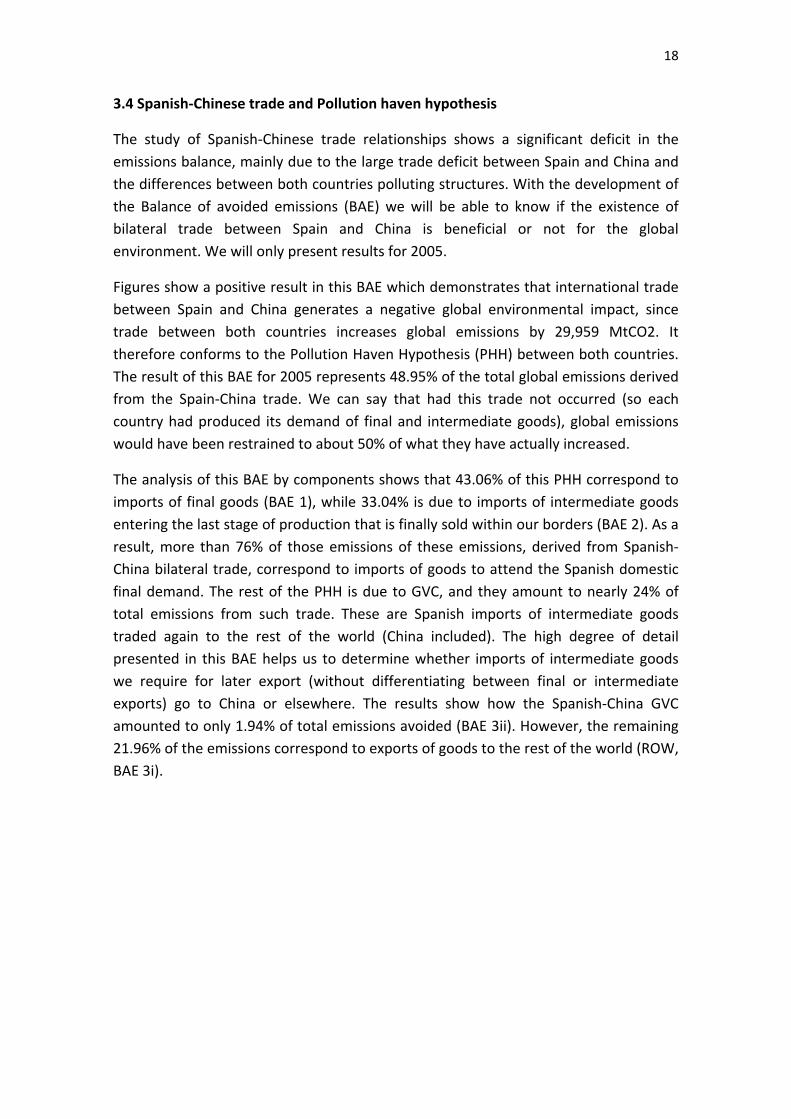
The analysis of this BAE by components shows that 43.06% of this PHH correspond to 

imports of final goods (BAE 1), while 33.04%  is due to  imports of  intermediate goods 

entering the last stage of production that is finally sold within our borders (BAE 2). As a 

result, more  than 76% of  those emissions of  these emissions, derived  from Spanish‐

China bilateral trade, correspond to  imports of goods to attend the Spanish domestic 

final demand. The rest of the PHH  is due to GVC, and they amount to nearly 24% of 

total  emissions  from  such  trade.  These  are  Spanish  imports  of  intermediate  goods 

traded  again  to  the  rest  of  the  world  (China  included).  The  high  degree  of  detail 

presented  in  this BAE helps us  to determine whether  imports of  intermediate goods 

we  require  for  later  export  (without  differentiating  between  final  or  intermediate 

exports)  go  to  China  or  elsewhere.  The  results  show  how  the  Spanish‐China  GVC 

amounted to only 1.94% of total emissions avoided (BAE 3ii). However, the remaining 

21.96% of the emissions correspond to exports of goods to the rest of the world (ROW, 

BAE 3i). 

 

 

 

 

 

 

19  

Figure  4:  Decomposition  of  Spanish‐China  Balance  of  avoided  emissions  (2005), 

thousands of tons. 

 

 

As described  in the section on methodology, by working with matrices and vectors of 

final demand and diagonalised emissions, we are able to obtain a BAE  in matrix form 

(23 x 23) for each component in the balance. This is why we can exhaustively analyse 

the balance by rows and by columns.  

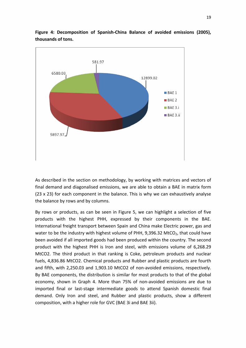
By  rows or products, as can be seen  in Figure 5, we can highlight a selection of  five 

products  with  the  highest  PHH,  expressed  by  their  components  in  the  BAE. 

International freight transport between Spain and China make Electric power, gas and 

water to be the industry with highest volume of PHH, 9,396.32 MtCO2, that could have 

been avoided if all imported goods had been produced within the country. The second 

product with  the  highest  PHH  is  Iron  and  steel, with  emissions  volume  of  6,268.29 

MtCO2.  The  third  product  in  that  ranking  is  Coke,  petroleum  products  and  nuclear 

fuels, 4,836.86 MtCO2. Chemical products and Rubber and plastic products are fourth 

and  fifth, with 2,250.03 and 1,903.10 MtCO2 of non‐avoided emissions,  respectively. 

By BAE components, the distribution is similar for most products to that of the global 

economy,  shown  in Graph  4. More  than  75%  of  non‐avoided  emissions  are  due  to 

imported  final  or  last‐stage  intermediate  goods  to  attend  Spanish  domestic  final 

demand.  Only  Iron  and  steel,  and  Rubber  and  plastic  products,  show  a  different 

composition, with a higher role for GVC (BAE 3i and BAE 3ii). 

20  

According to this analysis, we can conclude that the Spanish‐Chinese trade is based on 

energy and input‐intensive goods, or on goods that require intensively energy for their 

extraction and processing, as  Iron and  steel, or  transformed  from energy goods  like 

Rubber and plastic products. 

Figure 5: BAE analysis by rows, thousand tons. 

 

 

The  columns  or  sectors  analysis  provides  information  about  delocalising  sectors, 

showing  the  Spain‐China  trade PHH  sectoral  composition  accounting  for  goods  final 

destination,  

Figure 6 contains those sectors with higher PHH in 2005. It shows all the components 

within BAE  in order to differentiate the environmental effect of the different uses of 

traded goods. 

It  is  remarkable  the  textile  industry PHH, 5,143.53 MtCO2 non‐avoided, where most 

imported goods satisfy final demand (BAE1). Building is the second sector with higher 

PHH,  3,737.19  MtCO2  non‐avoided.  They  are  all  devoted  to  the  second  BAE 

component,  that  is, emissions embodied  in  imported  goods  that  fit  into  final  goods 

sold to domestic demand, (BAE2). The third sector  in BAE  importance  is Manufacture 

of transport equipment, with a PHH of 3,129.64 MtCO2 non‐avoided emissions that go 

mainly to GVC, more specifically as exports to the rest of the world (BAE3.i). The forth 

sector in PHH importance is Machinery and equipment, with a total of 2,849.60 MtCO2 

non‐avoided,  that  go mainly  to  final  demand.  The  fifth  sector  is Manufacturing  & 

recycling,  with  a  PHH  of  2,386.17  MtCO2  non‐avoided,  and  the  sixth  is  Electrical 

21  

machinery, with a PHH of 2153.27 MtCO2. The last two groups enter in the production 

of final goods. 

The results show that sectors with higher PHH are among the most intensive in energy 

use, similarly to the results of the rows analysis of Figure 5.  

Figure 6: BAE analysis by columns 

 

 

4. Conclusions  

The analysis  in this paper allows us to state that China has become a pollution haven 

for  the Spanish economy. Firstly, because  the emissions balance between  these  two 

countries shows a negative balance for Spain of 61,200 ktCO2, from a total of 62,000 

ktCO2  exchanged.  Secondly,  and more  important,  the  balance  of  avoided  emissions 

shows that almost 50% of those emissions, 29,000 ktCO2, are due to the existence of 

international  trade.  This  is  explained  by  the  high  polluting  intensity  of  the  Chinese 

economy  compared  to  Spain.  In  a world with  no  international  trade  each  country 

would have to produce  its  imports and that would have avoided those 29,000 ktCO2. 

When  producing  and  selling,  firms  neglect  the  environmental  impact  of  that 

production in both countries. 

The main  contribution of  this work  is  that  the methodology  and data used,  in  a bi‐

regional  context,  has  allowed  us  to  differentiate  our  BAE measure  by  components, 

depending on whether the goods traded were final or  intermediate, and on whether 

they attended domestic final demand or were re‐inserted in GVC through exports. The 

22  

four components of our equation are: BAE 1) final goods trade for both countries; BAE 

2)  trade of  final  round of  intermediate goods  to  serve  the domestic  final demand  in 

each country; trade of intermediate goods to serve the exported final demand of both 

countries (GVC), they can be to the Rest of the world (BAE 3.i) or to the country with 

which we trade bilaterally (BAE 3.ii). 

By means of  international  trade between Spain and China profits are generated and 

shared by entrepreneurs, consumers, workers and governments through taxes in both 

countries.  Nevertheless,  besides  these  profits  there  are  some  losses  due  to  the 

increase  of  CO2  emissions  that  generate  external  effects  for which  nobody  is  held 

responsible. These agents must become, up to a point, responsible if our objective is to 

reduce  the environmental  impact  from economic activity. Governments,  through  the 

design  of  appropriate  policies,  are  the  main  agent:  international  agreements  that 

progressively  incorporate  non‐Kyoto‐signatory  countries  in  the  line  of  Copenhagen, 

imposing  CO2  border  taxes,  promoting  renewable  energies  in  the  production  of 

electricity,  designing  ecological  labels  that  would  allow  consumers  to  identify  less 

polluting goods, etc. 

 

 

 

23  

Bibliography 

Ahmad, N. and Wyckoff, A., 2003. Carbon dioxide emissions embodied in international trade of goods. OECD Science, Technology and Industry Working Paper, 15. 

Antweiler, W., 1996. The pollution  terms of  trade. Economic  System Research, 8, 4, 361‐365. 

Azqueta,  D.,  Delacámara,  G.  y  Sotelsek,  D.,  2006.  Degradación  ambiental, endeudamiento externo y comercio internacional. Cuadernos Económicos de ICE, 71, 115‐132. 

Cadarso,  M.A.,  Gómez,  N.;  López,  L.A.  and  Tobarra,  M.A.,  2007.  El  papel  de  las multinacionales  en  la  deslocalización  y  la  especialización  vertical  de  la  industria  española. Revista de Economía Mundial, 16, 27‐55. 

Cadarso, M.A., Gómez, N.; López, L.A. and Tobarra, M.A., 2008. The EU enlargement and  the  impact  of  outsourcing  on  industrial  employment  in  Spain,  1993‐2003,  Structural Change and Economic Dynamics, 19 (1), 95‐108. 

Cadarso, M.A.,  Gómez,  N.;  López,  L.A.  and  Tobarra, M.A.,  2010.  CO2  emissions  of international  freight  transport  and  offshoring:  measurement  and  allocation,  Ecological Economics, 69 (8), 1682‐1694. 

Cadarso, M.A., Gómez, N.; López, L.A. and Tobarra, M.A., 2012. International trade and shared responsibility. An application to the Spanish economy. Ecological Economics, in press. 

Chen, Z. M., & Chen, G. Q., 2011. Embodied carbon dioxide emission at supra‐national scale: A coalition analysis for G7, BRIC, and the rest of the world. Energy Policy, 39(5), 2899‐2909. 

Copeland, B. R., & Taylor, M. S., 2004. Trade, Growth and the Environment. Journal of Economic Literature, 42(1), 7 ‐ 71. 

Cristea,  A.,  Hummels,  D.  and  Puzzelo,  L.,  2011.  Trade  and  the  Greenhouse  Gas Emissions  from  International  Freight  Transport,  paper  presented  at  the  ETSG  Conference Copenhagen, Denmark. 

Davis, S.  J., Peters, G. P., and Caldeira, K., 2011. The  supply  chain of CO2 emissions. www.pnas.org/cgi/doi/10.1073/pnas.1107409108 

DGA, 2011. Dirección General de Aduanas. In Agencia Tributaria. Gobierno de España. (online). 

Dietzenbacher,  E.,  &  Mukhopadhyay,  K.,  2007.  An  Empirical  Examination  of  the Pollution Haven Hypothesis  for  India:  Towards  a Green  Leontief  Paradox?  Environmental & Resource Economics, 36(4), 427‐449. 

Feenstra,  R.  C.,  1998.  Integration  of  trade  and  disintegration  of  production  in  the global economy. Journal of Economic Perspectives, 12, 31‐50. 

Felder, S. and Rutherford, T., 1993. Unilateral CO2 reductions and carbon  leakage: the consequences of  international  trade  in basic materials.  Journal of Environmental Economics and Management, 25, 162‐176. 

Ferng,  J.  J.,  2003.  Allocating  the  responsibility  of  CO2  over‐emissions  from  the perspectives of benefit principle and ecological deficit. Ecological Economics, 46, 121‐141. 

Gallego,  L.  y  Lenzen,  M.,  2005.  A  consistent  input–output  formulation  of  shared consumer and producer responsibility. Economic Systems Research, 17 (4), 365–391. 

24  

Gay, P. W. and Proops, J. L. R., 1993. Carbon‐dioxide production by the UK economy: an input‐output assessment. Applied Energy, 44, 113‐130. 

Gómez,  N.;  López,  L.A.  and  Tobarra,  M.A.,  2006.  Pautas  de  deslocalización  de  la industria española en el entorno europeo (1995‐2000):  la competencia de  los países de bajos salarios, Boletín del ICE, n. 2884, pp. 25‐41. 

Hummels,  D.,  Ishii,  J.  and  Yi,  K.M.,  2001.  The  nature  and  growth  of  vertical specialization in world trade. Journal of International Economics, 54 (1), 75‐96. 

IEA (2009) World energy outlook 2009. International Energy Agency (IEA), Paris. 

INE,  2005.  Contabilidad  nacional  de  España. Marco  input‐output.  Serie  1995‐2000. Madrid, Instituto Nacional de Estadística. 

INE, 2006. Cuentas  Satélite  sobre  emisiones Atmosféricas.  Serie 1995‐2000. Madrid, Instituto Nacional de Estadística. 

INE, 2008. Cuentas Satélite sobre Emisiones Atmosféricas. 

International Energy Agency (IEA), 2001. CO2 from fuel combustion, OECD, Paris. 

IPCC,  1997.  Revised  1996  IPCC  guidelines  for  national  greenhouse  gas  inventories: reporting instructions. Cambridge University Press, Cambridge, UK. 

Johnson, R. C., & Noguera, G., 2011. Accounting for intermediates: Production sharing and trade in value added. Journal of International Economics, in press. 

Kanemoto,  K.,  Lenzen,  M.,  Peters,  G.P.,  Moran,  D.D.  and  Geschke,  A.,  2012. Frameworks  for  comparing  emissions  associated  with  production,  consumption  and international trade, Environmental Science and Technology, 46, 172‐179. 

Lenzen,  M.,  2008.  Consumer  and  producer  environmental  responsibility:  a  reply. Ecological economics, 66, 547‐550. 

Lenzen, M., Murray, J., Sack, F. and Wiedman, T., 2007. Shared producer and consumer responsibility – Theory and practice. Ecological Economics, 61, 27‐42.  

Lenzen, M.; Pade, L.L. and Munksgaard, J., 2004. CO2 multipliers in multi‐region input‐output models. Economic System Research, 16, 4, 391‐412. 

Leontief, W. and Ford, D., 1972. Air pollution and  the economic  structure: empirical results of  input‐output  computations,  in Brody A., Carter A.  (Eds.),  Input‐output  techniques, Amsterdam, North‐Holland, 9‐30. 

Leontief,  W.,  1941.  The  structure  of  the  American  economy,  1919‐39.  New  York, Oxford University Press.  

Leontief,  W.,  1970.  Environmental  Repercussions  and  the  Economic  Structure:  An Input‐Output Approach. The Review of Economics and Statistics, 52, 3, 262‐71. 

Levinson,  A.,  2009:  “Technology,  International  Trade,  and  Pollution  from  U.S. Manufacturing”, American Economic Review, 99 (5), 2177–92. 

Levinson, A.,  2010. Offshoring  Pollution:  Is  the United  States  Increasingly  Importing Pollution Goods? Review of Environmental Economics and Policy, 4(1), 63‐83. 

Li, Y., & Hewitt, C. N., 2008. The effect of trade between China and the UK on national and global carbon dioxide emissions. Energy Policy, 36, 1907‐1914. 

Lin, B. and Sun, C., 2010. Evaluating carbon dioxide emissions in international trade of China. Energy Policy, 38 (1), pp. 613‐628. 

25  

Liu, X.,  Ishikawa, M., Wang, C., Dong, Y., & Liu, W., 2010. Analyses of CO2 emissions embodied in Japan ‐ China trade. Energy Policy, 38(3), 1510 ‐ 1518. 

Machado, G., Schaeffer, R. and Worrell, E., 2001. Energy and carbon embodied  in the international trade of Brazil: an input‐output approach. Ecological Economics, 39, 409‐424. 

McGregor, P.G.,  Swales,  J.K.  and  Turner, K., 2008.  The CO2  ‘trade balance’ between Scotland and the rest if the UK: performing a multi‐region environmental input‐output analysis with limited data. Ecological Economics, 66, 662‐673. 

Minx,  J.C.; Wiedmann,  T.; Wood,  R.;  Peters,  G.P.;  Lenzen, M.;  Owen,  A.;  Scott,  K.; Barrett,  J.;  Hubacek,  K.;  Baiocchi,  G.;  Paul,  A.;  Dawkins,  E.;  Briggs,  J.;  Guan,  D.;  Suh,  S.; Ackerman,  F.,  2009.  Input–output  analysis  and  carbon  footprinting:  an  overview  of applications, Economic Systems Research, 21(3), 187‐216. 

Mongelli,  I.;  Tassielli,  G.  and  Notarnicola,  B.,  2006.  Global  warming  agreements, international trade and energy/carbon embodiments: an input–output approach to the Italian case. Energy Policy, 34 (1), 88‐100. 

Munksgaard, J. and Pedersen, K., 2001. CO2 accounts for open economies: producer or consumer responsibility? Energy Policy, 29, 327‐334. 

Muradian, R., O’Connor, M. and Martinez‐Alier, J., 2002. Embodied pollution  in trade: estimating  the  ‘environmental  load  displacement’  of  industrialised  countries,  Ecological Economics, 41 (1), 51‐67. 

NBSC,  2011.  China  Stastistical  Yearbook.  In  National  Bureau  of  Statistics  of  China (online). 

OECD, 2005. Input ‐ Output Framework. 

OECD, 2007. Moving Up the Value Chain: Staying Competitive in the Global Economy. A Synthesis Report on Global Value Chains, OECD, Paris. 

OECD, 2011. Towards Green Growth – Monitoring Progress: OECD  Indicators. OECD, may. 

Paltsev, S., 2001. The Kyoto protocol: regional and sectoral contributions to the carbon leakage. The Energy Journal, 22 (4), 53‐79. 

Pasinetti,  P.  L.,  1973.  The  notion  of  vertical  integration  in  economic  analysis, Metroeconomica, 25, 1‐29. 

Peters, G. P. and Hertwich, E. G., 2006a. Pollution embodied  in trade: the Norwegian case. Global Environmental Change, 16, 379‐389. 

Peters, G.  P.  and Hertwich,  E. G.,  2006b.  The  importance  of  imports  for  household environmental impacts. Journal of Industrial Ecology, 10 (3), 89‐109. 

Peters, G.  P.  and Hertwich,  E. G.,  2008a.  CO2  embodied  in  international  trade with implications  for  global  climate  policy.  Environmental  Science  and  Technology,  42  (5),  1401‐1407. 

Peters, G. P. and Hertwich, E. G., 2008b. Post‐Kyoto gas inventories: production versus consumption. Climatic Change, 86, 51‐66. 

Peters, G. P., 2008. From production‐based  to  consumption‐based national emission inventories. Ecological Economics, 65, 13‐23. 

Peters,  G.  P.,  Weber,  C.  L.,  Guan,  D.,  &  Hubacek,  L.,  2007.  China´s  growing  CO2 Emissions  ‐  A  race  between  Increasing  Consumption  and  Efficiency  Gains  ‐.  Environmental Science and Technology, 41(17). 

26  

Roca, J. and Serrano, M., 2007a. Income growth and atmospheric pollution in Spain: an input‐output approach. Ecological Economics, 63 (1), 230‐242. 

Sánchez‐Chóliz, J. and Duarte, R., 2004. CO2 emissions embodied in international trade: evidence for Spain. Energy Policy, 32, 1999‐2005. 

Serrano, M. and Dietzenbacher, E., 2010. Responsibility and trade emission balances: an evaluation of approaches. Ecological Economics, 69, 2224‐2232. 

Su, B. and Ang, B.W., 2010. Input‐output analysis of CO2 emissions embodied in trade: the effects of spatial aggregation, Ecological Economics, 70, 10‐18. 

Su,  B.  and  Ang,  B.W.,  2011.  Multi‐region  input‐output  analysis  of  CO2  emissions embodied in trade: the feedback effects. Ecological Economics, 71, 42‐53. 

Su,  B.,  Huang,  H.C.,  Ang,  B.W.,  and  Zhou,  P.,  2010.  Input‐output  analysis  of  CO2 emissions embodied in trade: the effects of sector aggregation, Energy Economics, 32 (1), 166‐175. 

Turner,  K.,  Lenzen,  M.,  Wiedmann,  T,  and  Barrett,  J.,  2007.  Examining  the  global environmental  impact  of  regional  consumption  activities—Part  1:  A  technical  note  on combining input–output and ecological footprint analysis. Ecological Economics, 62, 37‐44. 

U.S.  EIA  (2009)  International  energy  outlook  2009.  U.S.  Energy  Information Administration (EIA), Washington, DC. 

UNFCCC,  2011.  Greenhouse  Gas  Inventory  Data.  United  Nations  Framework Conventions on Climate Change. Spanish Data. GHG Inventory Submission of 2011. 

Wiedmann  T.,  Lenzen,  M.,  Turner,  K,  and  Barret,  J.,  2007.  Examining  the  global environmental  impact  of  regional  consumption  activities  –  Part  2:  Review  of  input‐output models for the assessment of environmental impacts embodied in trade. Ecological Economics, 61, 15‐26. 

Wiedmann  T., Minx,  J., Barrett,  J.,  and Wackernagel, M., 2006. Allocating  ecological footprints  to  final  consumption  categories with  input–output analysis. Ecological economics, 56, 28‐48. 

Wiedmann,  T., 2009. A  review of  recent multi‐region  input–output models used  for consumption‐based emission and resource accounting, Ecological Economics, 69, 211‐222. 

WTO‐UNEP,  2009.  Trade  and  Climate  Change.  World  Trade  Organization  /  United Nations Environment Programme Report.