Indirect Utility Maximization under Risk:

A Heterogeneous Panel Application

Yucan Liu and C. Richard Shumway *

Selected Paper prepared for presentation at the Western Agricultural Economics Association Annual Meeting, San Francisco, California, July 6-8, 2005

Copyright 2005 by [Yucan Liu and C. Richard Shumway]. All rights reserved. Readers may make verbatim copies of this document for non-commercial purposes by any means, provided that this copyright notice appears on all such copies.

* Yucan Liu: Ph.D. Student, School of Economic Sciences, Washington State University, Pullman, WA

99164-6210. Phone: 509-338-4902, Email: yucanliu@yahoo.com.

C. Richard Shumway: Professor, School of Economic Sciences, Washington State University, Pullman, WA

99164-6210. Phone: 509-335-1007, Email: shumway@wsu.edu.

1

Indirect Utility Maximization under Risk:

A Heterogeneous Panel Application

Abstract

The curvature properties of the indirect utility function imply a set of refutable implications in

the form of comparative static results and symmetric relations for the competitive firm operating

under uncertainty. These hypotheses, first derived and empirically tested under output price

uncertainty by Saha and Shumway (1998), are extended in this article to the more general case of

both price and quantity uncertainty and result in an important theoretical finding. Using recently

developed techniques for testing unit root and cointegration in heterogeneous panels, we develop

a model of U.S. agricultural production based on the time series properties of a panel of

state-level data and contrast test implications with those resulting from a traditional model that

presumes stationarity in all variables. Although differing in specific outcomes, the empirical tests

of the refutable hypotheses render the same conclusions for both models: we fail to reject most

refutable hypotheses under output price and output quantity risk, symmetry conditions implied

by a twice-continuously-differentiable indirect utility function are rejected, two restrictive risk

preference hypotheses are also rejected, and, at individual observations, data are generally

consistent with most (but not all) of the hypotheses implied by individual states acting as though

they were expected utility-maximizing firms.

Key words: refutable implications, risk and uncertainty, panel unit root, panel cointegration

2

Indirect Utility Maximization under Risk:

A Heterogeneous Panel Application

Because of the long time periods between commitment of resources and generation of

marketable output in production agriculture, a high level of uncertainty is associated with many

production decisions. Because producers frequently have few options available to significantly

alter input combinations after the decision is made to produce a commodity, opportunities to

reduce the adverse consequences of risk are often limited in the short run. Consequently,

economists concerned about decision making in production agriculture have had a long history

of considering the impact of risk and uncertainty.

Building on the early work of Sandmo (1971) and Batra and Ullah (1974), who

developed the theory of the competitive firm under output price uncertainty, agricultural

economists have examined firm operations and developed testable firm models under various

sources of risk. The pioneering work of Pope (1980) derived testable hypotheses expressed in

symmetry and homogeneity results under constant absolute risk aversion and price uncertainty.

His symmetry results proved simple enough for empirical application under certain classes of

utility functions (Antonovitz and Roe 1986). Chavas and Pope (1985) extended Pope’s work by

examining price uncertainty within a general risk preference framework which facilitated

empirical tests of firm behavior under the expected utility hypothesis. Paris (1988) analyzed the

competitive entrepreneur under output and input price uncertainty in a long-run scenario. Dalal

(1990) derived additional symmetry conditions for empirical application under price risk.

Adrangi and Raffiee (1999) derived testable implications within a comparative statics framework

for the competitive firm operating under output and input price uncertainty.

3

A number of studies have also provided empirical tests for behavioral hypotheses of the

firm operating under risk. For example, Chavas and Holt (1990) developed an acreage supply

response model consistent with expected utility maximization and empirically tested the

symmetry restrictions using annual time-series data for U.S. corn and soybean acreage decisions.

They found empirical evidence for the symmetry conditions and decreasing absolute risk

aversion (DARA) on the part of the producer. Later they (Chavas and Holt 1996) tested the

economic implications of producer behavior under price and production risk in U.S. corn and

soybean acreage response decisions. The null hypothesis of CARA was rejected and evidence

was again found to support DARA. Theoretical and functional form deficiencies in the

Chavas-Holt analysis were addressed by Satyanarayan (1999), who extended previous works to

the firm operating under domestic price and exchange rate uncertainty.

Park and Antonovitz (1992a, b) derived and empirically tested the reciprocity conditions

linking optimal output and hedging decisions for the competitive firm that uses hedging to

manage price uncertainty. They concluded that the symmetric results as well as constant absolute

risk aversion (CARA) for their California feedlot could not be rejected. Dalal (1994) alleged a

misspecification, criticized their conclusions, and developed a more general formulation using

the envelope theorem and derivatives of the indirect expected utility function.

Saha and Shumway (1998) derived general refutable implications from the first-order and

second-order curvature properties of the indirect utility function under output price uncertainty

and empirically tested each postulate for a sample of Kansas wheat producers. They failed to

reject any of the implications of expected utility maximization for their data set but rejected

restrictive risk attitudes including both CARA and risk neutrality.

4

Several studies have recently investigated firm behavior under risk using pooled

cross-sectional time-series data (e.g., Saha and Shumway 1998; Lien and Hardaker 2001;

Kumbhakar 2002; Kumbhakar and Tveteras 2003; Roosen and Hennessy 2003). Using panel

data has several benefits for empirical analysis. For example, it enlarges the sample size,

enhances the power of statistical tests, and facilitates analysis of dynamic properties of

relationships. However, a daunting challenge arising from both time series and panel data

regressions is the possibility that variables involved in the regressions are nonstationary. Unless a

linear combination of nonstationary variables is stationary, i.e., the variables are cointegrated,

use of ordinary regression estimators may lead to spurious results (Phillips 1986; Engle and

Granger 1987).

Traditional tests of unit roots and cointegration have low power against the alternate

hypothesis of stationarity in small and moderate sized samples. Consequently, failure to reject

the hypothesis of a unit root in the series or in the linear combination of variables may occur

because of the low power of the tests as well as failure of the data to satisfy the necessary

conditions. Whatever the cause, failure to find stationarity in each series or in a linear

combination of the series gives the analyst pause when seeking to estimate long-run relationships

in the data. Recent developments in time-series econometrics that combine time-series and

cross-sectional information have provided important possibilities for surmounting this dilemma.

Panel data increase the power of unit root and cointegration tests even though the length of the

time series is unaffected. Consequently, confidence in time series test conclusions is increased by

use of panel data.

Although pooled cross-sectional time-series data has been frequently used to examine

firm behavior under risk, it appears that none has examined the time-series properties of the

5

panel data. Consequently, reported results are subject to the possibility of the spurious regression

problem. The current research seeks to at least partially fill this void by employing recent

advances in the econometrics literature designed to test for panel unit roots (i.e. Im, Pesaran, and

Shin 1997) and panel cointegration (i.e. Pedroni 1999).1 These panel tests allow for both

parametric and dynamic heterogeneity across groups and are considerably more powerful than

conventional methods (Harris and Tzavalis 1999). Besides its unique application to firm

behavior under risk, this investigation joins only a small number of other studies in reporting

empirical applications of panel cointegration techniques to a heterogeneous panel with multiple

regressors.2

With this background, the objectives of this article are to: (a) extend the previous

theoretical work by careful derivation of refutable and testable implications of the indirect utility

function under both output price and quantity risk, (b) demonstrate that one previously

maintained hypothesis is not a necessary condition for the derived implications, (c) empirically

test the derived implications as well as a set of hypotheses about the nature of risk aversion

practiced by producers using a traditional model in which stationarity of the data is implicitly

assumed and time is included as a proxy for technical change, (d) examine the time-series

properties of variables involved in a system of input demand equations by employing recent

developments in panel unit root and panel cointegration techniques, (e) develop a model for

input demands consistent with the time series test results and with technical change proxied by

public research expenditures, and (f) contrast important inferences from hypothesis test results

from this model with those from the traditional model.

The plan of this article is as follows. The next section gives a brief overview of the

behavioral theory implied by curvature properties of the indirect utility function and derives a set

6

of testable hypotheses. The following section discusses our econometric model and introduces

the panel testing methodologies employed in this article. Time series properties of our data based

on panel unit root and cointegration tests are then reported along with empirical results of the

refutable hypotheses from both models. Conclusions are presented in the last section.

Theoretical Model

Traditionally, the introduction of price uncertainty into the theory of the competitive firm has

been approached within an expected utility framework. The seminal works of Arrow (1965) and

Pratt (1964) defined preferences of expected utility-maximizing decision makers over final

wealth. Despite their unambiguous reference to final wealth, much of the analysis of risk taking

behavior of agricultural producers, beginning with Sandmo (1971), has used profit rather than

wealth as the argument of utility (Meyer and Meyer 1998). Profit is the appropriate argument

only if sources of wealth other than profit are nonrandom and held fixed. Since we do not wish to

impose nonrandom constraints on other sources of wealth, we use wealth as the argument of

utility in the following theoretical model. Therefore, the firm is assumed to maximize its

expected utility of random wealth.

Following Feder (1977) and Saha and Shumway (1998), we assume that a competitive

firm’s random wealth W can be structured as a nonrandom part Z(∙), a random component S(∙),

and nonrandom initial (beginning of period) wealth endowment I:

(1) ; , ; ; IW Z S � �x x

where x =(x1, x2,…, xn)’ is an 1n vector of decision variables, is a random variable vector,

β is a parameter vector, and · denotes the additional parameters concealed in Z(∙) and S(∙). The

parameters, β, only enter the nonrandom part of wealth, Z(∙), but not the random part S(∙).

7

Although we later demonstrate that it is unnecessary for our refutable implications to hold under

output price and output quantity risk, we initially maintain the standard expectation:

(2) E ; , 0S �x

where E denotes the expectation operator.

Conditional on twice-differentiable functions of Z and S, the expectation of random

wealth defined by (1) and (2) can be written as:

(3) E ; , I E ; ; ; , IW W Z S Z � � �x x x .

Refutable Implications of the Indirect Utility Function

For a competitive firm whose objective is to maximize the expected utility of random

wealth specified by (1), the indirect utility function is defined by:

(4) ; I, E ; , ; ; IV max U Z S � � �x x ,

where U(∙) represents the von Neumann Morgenstern utility function, which is increasing in

wealth, therefore is increasing in nonrandom part of wealth, Z(x; β, ∙). Let x*(β, I, ∙) denote the

optimal input variables which are determined by (4). Under the assumptions of (1) and (2), the

indirect utility function defined by (4) implies the following propositions (Saha and Shumway

1998):

Proposition 1: The indirect utility function defined by (1) has the following first-order curvature

properties:

(i) Increasing in I,

(ii) Increasing (decreasing) in β if Z is increasing (decreasing) in β.

Proposition 2: The second-order curvature properties of the indirect utility function indicate:

(i) V quasiconvex in β and I if Z is convex in β,

8

(ii) V quasiconvex in β and I symmetric and positive semidefinite (SPSD),

where * *IZ Z Z x x x .3

Corollary: Under risk neutrality or CARA, xI*=0, and Z convex in β *Z Z x x is SPSD.

Obviously, V(β; I, ∙) is increasing in I. Proposition 1(ii) indicates that the first-order

curvature properties of the indirect utility function corresponding to β can be revealed by the

first-order curvature characters of the nonrandom part of wealth Z(x; β, ∙). Proposition 2(i)

implies the fundamental second-order curvature properties of the indirect utility function which

can be explored by observing the properties of the second-order curvature of Z(x; β, ∙). By

proposition 2(i), V(β; I, ∙) is quasi-convex in β if Z is convex in β. This property implies and is

implied by the testable postulates contained in proposition 2(ii). In proposition 2(ii), the

symmetric and positive semi-definite (SPSD) matrix, , which contains the comparative static

and reciprocity results demonstrating the firm behaviors, includes the complete set of the

refutable implications for the competitive firm under risk. Most importantly, propositions 1 and 2

do not rely on specific forms of U(∙) that would otherwise impose an explicit risk preference

(Love and Buccola 1991; Saha Shumway and Talpaz 1994). When combined with the

empirically testable curvature properties of Z(x; β, ∙), they allow us to test the behavioral

postulates without assuming a specific functional form for the indirect utility function.

These refutable propositions derived by Saha and Shumway (1998) have been

empirically tested only under output price uncertainty. One important theoretical contribution of

this article, the importance of which will be explained in the next section, is to demonstrate that

the propositions hold even without assumption (2). From the proof in Saha and Shumway (1998),

it is obvious that proposition 1 and proposition 2(ii) aren’t conditioned on assumption (2), and all

that is needed for them to hold is assumption (1). We refer readers to Saha and Shumway (1998)

9

for the details. Before proving that proposition 2(i) holds without assumption (2), we claim the

following result.

Claim. The firm’s optimization problem defined in (4) is equivalent to a constrained

optimization problem where x and W are jointly chosen. Defining ,Wk x and λ = {β, I},

then:

(5)

max E ; , ; ; I

max E ; ; E ; ; | ; , E ; ; I

x

k

V U Z S

V U W S S W Z S

� �

� � � �

x x

x x x x.

Proof: First, we demonstrate that the constraint, ( ;β, ) E[ ( ; ; )] IW Z S x x , will be

binding for all optimal values of and W x . Suppose the constraint is not binding, then there

must exist some parameter values 0 0 0 0 0 0{ , } and {β , I }W k x λ such that 0 0 0{ , } Wk x

and 0 0 0{β , I }λ maximize the indirect utility, given by (5), with the following condition

(6) 0 0 0 0 0x ; , E ; ; IW Z S x � � .

Therefore, there exists some 0'W W such that

(7) 0 0 0 0' E ' ( ;β , ) I E ( ; ; ),W W Z S x x

which implies 0{ , '}Wx is feasible.

Since the utility function is increasing in wealth, we have

(8) 0 0 0 0 0E ( ' ( ; ; ) E[ ( ; ; )]) E ( ( ; ; ) E[ ( ; ; )])U W S S U W S S x x x x ,

which contradicts the fact that 0 0 0 0 0 0{ , } and {β , I }W k x λ maximize the indirect utility.

Thus, the constraint is binding for all optimal values of and k λ , and the claim is proved by

substituting the binding constraint E ( ;β, ) I E ( ; ; )W W Z S x x into (5).

10

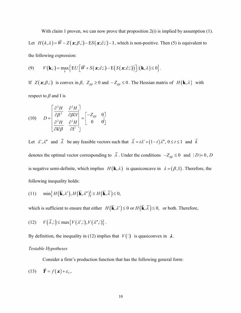
With claim 1 proven, we can now prove that proposition 2(i) is implied by assumption (1).

Let , ; , E ; ; IH k W Z S � �x x , which is non-positive. Then (5) is equivalent to

the following expression:

(9) , max E ; ; E ; ; | , 0k

V U W S S k k � � �x x .

If ; ,Z �x is convex in , 0 and 0Z Z . The Hessian matrix of ,H k with

respect to and I is

(10)

2 2

2

2 2

2

0

0 0

I I

H HZI

DH H

Let , and be any feasible vectors such that 1 , 0 1t t t and k

denotes the optimal vector corresponding to . Under the conditions 0Z and | | 0D , D

is negative semi-definite, which implies ,H k is quasiconcave in , I . Therefore, the

following inequality holds:

(11) min , , , , 0,H H H k k k

which is sufficient to ensure that either , 0 or , 0,H H k k or both. Therefore,

(12) , max , , ,V V V � � � .

By definition, the inequality in (12) implies that V � is quasiconvex in λ .

Testable Hypotheses

Consider a firm’s production function that has the following general form:

(13) ,Yf Y x

11

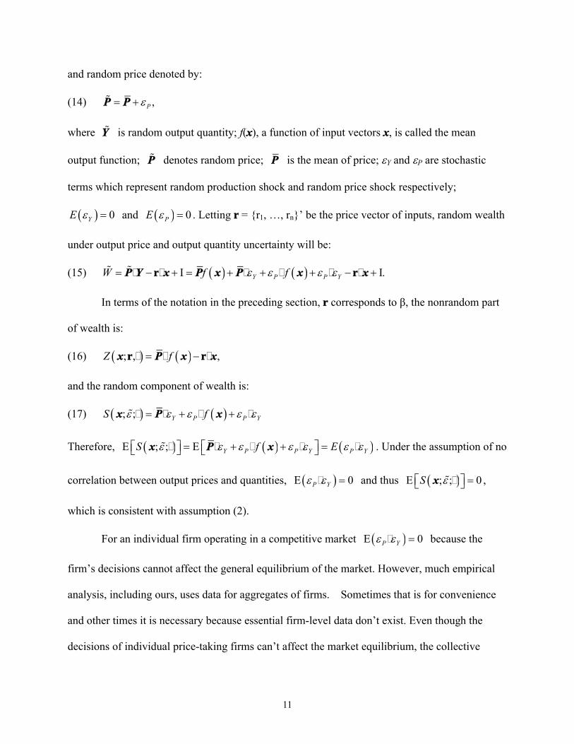
and random price denoted by:

(14) ,P P P

where Y is random output quantity; f(x), a function of input vectors x, is called the mean

output function; P denotes random price; P is the mean of price; Y and P are stochastic

terms which represent random production shock and random price shock respectively;

0YE and 0PE . Letting r = {r1, …, rn}’ be the price vector of inputs, random wealth

under output price and output quantity uncertainty will be:

(15) I I.Y P P YW f f r r � � � � � �P Y x P x P x x

In terms of the notation in the preceding section, r corresponds to β, the nonrandom part

of wealth is:

(16) ; , ,Z f r r� � �x P x x

and the random component of wealth is:

(17) ; ; Y P P YS f � � � �x P x

Therefore, E ; ; E Y P P Y P YS f E � � � � �x P x . Under the assumption of no

correlation between output prices and quantities, E 0P Y � and thus E ; ; 0S �x ,

which is consistent with assumption (2).

For an individual firm operating in a competitive market E 0P Y � because the

firm’s decisions cannot affect the general equilibrium of the market. However, much empirical

analysis, including ours, uses data for aggregates of firms. Sometimes that is for convenience

and other times it is necessary because essential firm-level data don’t exist. Even though the

decisions of individual price-taking firms can’t affect the market equilibrium, the collective

12

decisions of many firms can. Thus, since we have demonstrated that assumption (2) is

unnecessary for any of the previous implications to hold, it is clear that we can make use of

aggregate data, if necessary, to conduct empirical tests of both propositions.

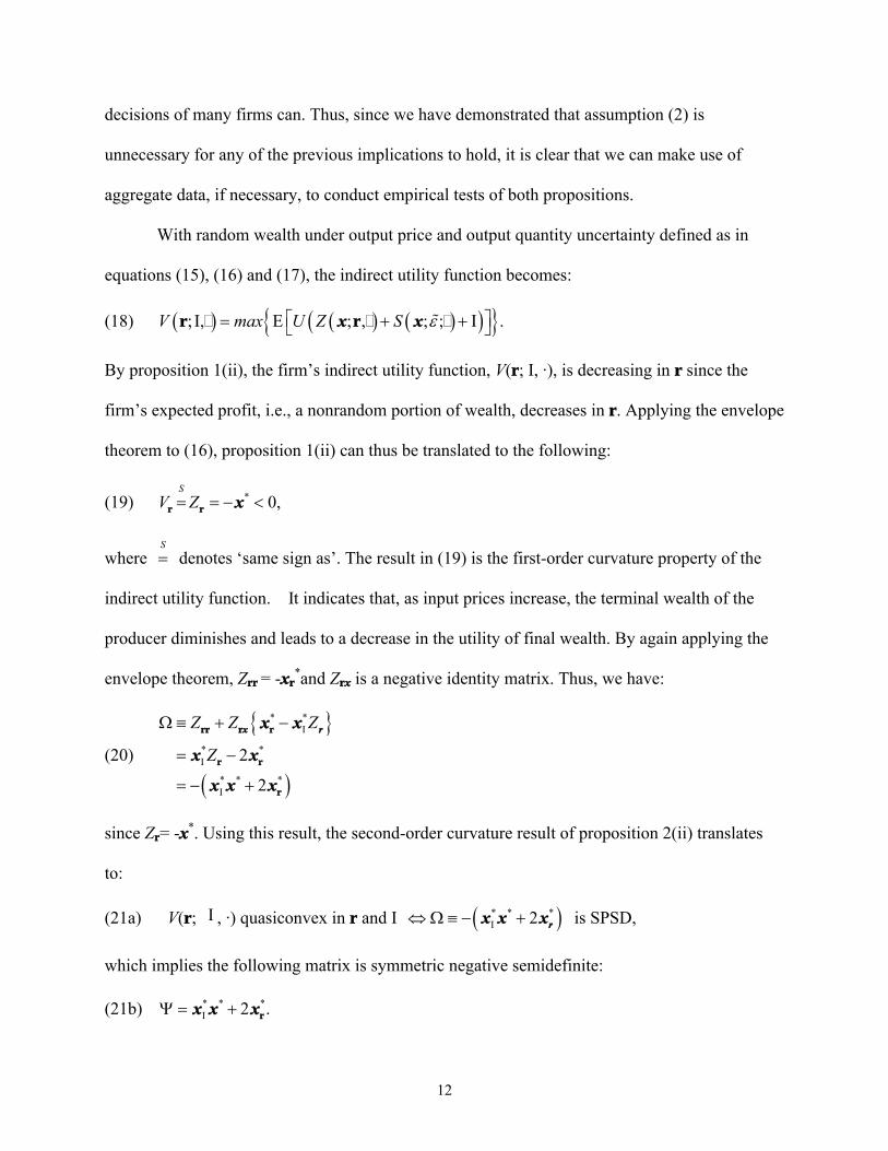
With random wealth under output price and output quantity uncertainty defined as in

equations (15), (16) and (17), the indirect utility function becomes:

(18) ; I, E ; , ; ; I .V max U Z S r r � � �x x

By proposition 1(ii), the firm’s indirect utility function, V(r; I, ∙), is decreasing in r since the

firm’s expected profit, i.e., a nonrandom portion of wealth, decreases in r. Applying the envelope

theorem to (16), proposition 1(ii) can thus be translated to the following:

(19) * 0,S

V Z r r x

where S

denotes ‘same sign as’. The result in (19) is the first-order curvature property of the

indirect utility function. It indicates that, as input prices increase, the terminal wealth of the

producer diminishes and leads to a decrease in the utility of final wealth. By again applying the

envelope theorem, Zrr = -xr*and Zrx is a negative identity matrix. Thus, we have:

(20)

* *I

* *I

* * *I

2

2

Z Z Z

Z

rr r r

r r

r

x rx x

x x

x x x

since Zr= -x*. Using this result, the second-order curvature result of proposition 2(ii) translates

to:

(21a) V(r; I , ∙) quasiconvex in r and I * * *I 2 rx x x is SPSD,

which implies the following matrix is symmetric negative semidefinite:

(21b) * * *I 2 . rx x x

13

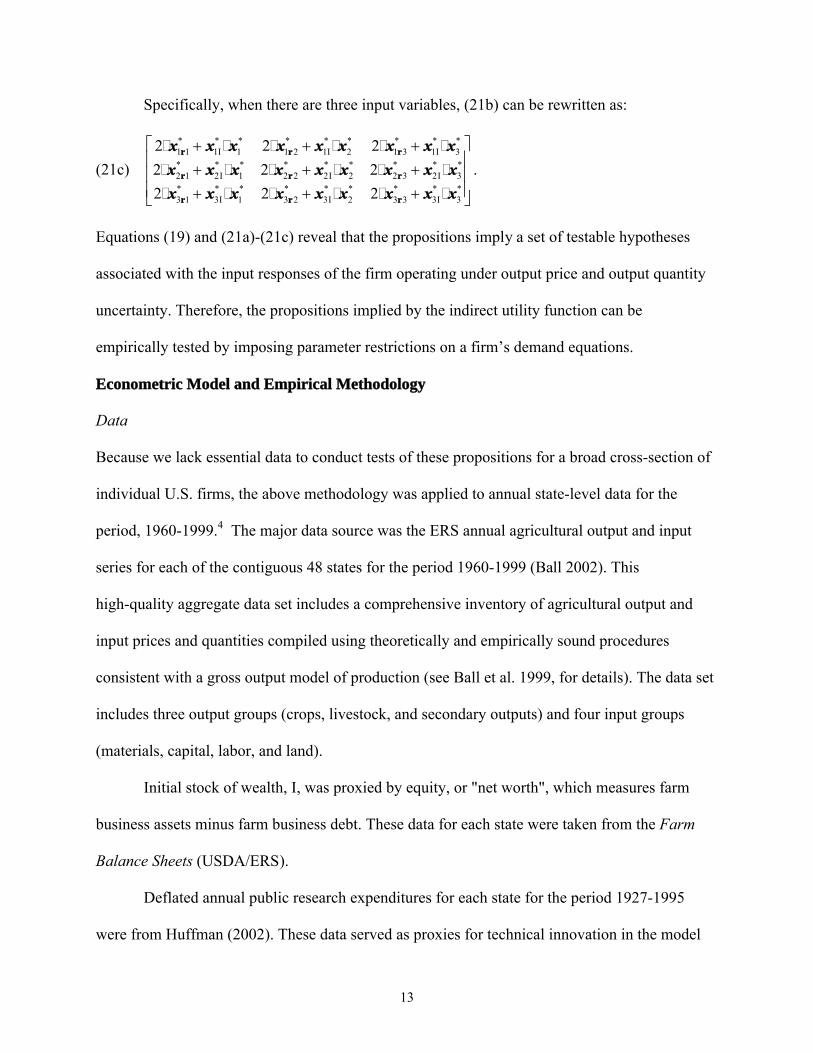
Specifically, when there are three input variables, (21b) can be rewritten as:

(21c)

* * * * * * * * *1 1 1I 1 1 2 1I 2 1 3 1I 3

* * * * * * * * *2 1 2I 1 2 2 2I 2 2 3 2I 3

* * * * * * * * *3 1 3I 1 3 2 3I 2 3 3 3I 3

2 2 2

2 2 2

2 2 2

r r r

r r r

r r r

� � � � � �

� � � � � �

� � � � � �

x x x x x x x x x

x x x x x x x x x

x x x x x x x x x

.

Equations (19) and (21a)-(21c) reveal that the propositions imply a set of testable hypotheses

associated with the input responses of the firm operating under output price and output quantity

uncertainty. Therefore, the propositions implied by the indirect utility function can be

empirically tested by imposing parameter restrictions on a firm’s demand equations.

Econometric Model and Empirical Methodology

Data

Because we lack essential data to conduct tests of these propositions for a broad cross-section of

individual U.S. firms, the above methodology was applied to annual state-level data for the

period, 1960-1999.4 The major data source was the ERS annual agricultural output and input

series for each of the contiguous 48 states for the period 1960-1999 (Ball 2002). This

high-quality aggregate data set includes a comprehensive inventory of agricultural output and

input prices and quantities compiled using theoretically and empirically sound procedures

consistent with a gross output model of production (see Ball et al. 1999, for details). The data set

includes three output groups (crops, livestock, and secondary outputs) and four input groups

(materials, capital, labor, and land).

Initial stock of wealth, I, was proxied by equity, or "net worth", which measures farm

business assets minus farm business debt. These data for each state were taken from the Farm

Balance Sheets (USDA/ERS).

Deflated annual public research expenditures for each state for the period 1927-1995

were from Huffman (2002). These data served as proxies for technical innovation in the model

14

based on the time series properties of the data. It has been showed that research expenditures can

affect technology, or the nature of the production function, at least seven years later and

sometimes as long as 30 years later (Chavas and Cox 1992; Pardey and Craig 1989). Akaike’s

Information Criterion (AIC) was used to select the optimal lag on public research expenditures.

Lagged output prices were used as proxies for expected output prices. Lagged equity was

used as a proxy for initial (beginning period) wealth. To partially mitigate the effects of trending

and autocorrelated data, expected output prices, equity, and current input prices were normalized

by the price of land. To reduce heteroskedasticity and to permit estimation of identical

non-intercept coefficients for all states in the panel data set, input quantities, normalized equity,

and deflated research expenditures were scaled by the quantity of land.5

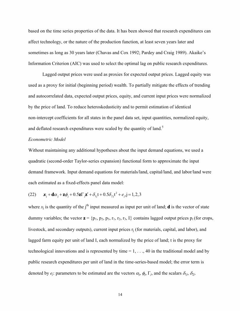
Econometric Model

Without maintaining any additional hypotheses about the input demand equations, we used a

quadratic (second-order Taylor-series expansion) functional form to approximate the input

demand framework. Input demand equations for materials/land, capital/land, and labor/land were

each estimated as a fixed-effects panel data model:

(22) 2j j j j 1j 2 j j0.5 t 0.5 t ,j 1,2,3e d z z zx

where xj is the quantity of the jth input measured as input per unit of land; d is the vector of state

dummy variables; the vector z = {p1, p2, p3, r1, r2, r3, I} contains lagged output prices pi (for crops,

livestock, and secondary outputs), current input prices rj (for materials, capital, and labor), and

lagged farm equity per unit of land I, each normalized by the price of land; t is the proxy for

technological innovations and is represented by time = 1, . . ., 40 in the traditional model and by

public research expenditures per unit of land in the time-series-based model; the error term is

denoted by ej: parameters to be estimated are the vectors j, j, j, and the scalars 1j, 2j.

15

For each individual equation in the demand system specified by (22), fixed effects across

cross-sectional observations were considered. So that all refutable implications under output

price and output quantity risk contained in (19) and (21a)-(21c) could be tested, no restrictions

were imposed on the estimated parameters across the equations.

Since stationarity of all variables is implicitly assumed when equation (22) is estimated

without first examining their time-series properties, the results of the traditional model may be

misleading. In the time-series-based model, we checked whether any of the variables contain unit

roots, and if they do, whether a linear combination of the variables as represented in equation (22)

also have a unit root (i.e., are not cointegrated). If they are cointegrated, a valid long-run

relationship can be represented by equation (22). Variables are cointegrated if they are stationary

after differencing and no unit root exists in the residuals (Engle and Granger, 1987). If all

nonstationary variables in equation (22) are cointegrated, the equation represents a structural

rather than a spurious relationship.

Unit Root Tests in Panel Data

The most common procedure used to test for a unit root in a data series is the augmented

Dickey-Fuller (ADF) test. The null hypothesis of this test is nonstationarity. Given the small

span of our time series (40 annual observations), conventional ADF tests conducted on each

individual state series can have very low power and lead to seriously misguided conclusions. The

preferred choice is to apply a panel unit root test.

Several procedures have been proposed to test for the null hypothesis of nonstationarity

in panels. Quah (1992, 1994) developed a test for a unit root in panel data subject to

homogeneous dynamics. Levin and Lin (1993) generalized this method to allow for fixed effects,

individual deterministic trends, and heterogeneous serially correlated errors. However, the

16

alternative hypothesis only allowed for the possibility of identical first-order autoregressive

coefficients in all series. To allow for residual serial correlation and heterogeneous

autoregressive coefficients across groups, Im, Pesaran, and Shin (1997) (hereafter IPS) proposed

using an average of the ADF tests. Monte Carlo experiments showed that the IPS test

outperforms Levin and Lin's test, especially having greater power and better small-sample

properties (Im, Pesaran, and Shin 1997). Consequently, the IPS test is the panel unit root test we

employ.

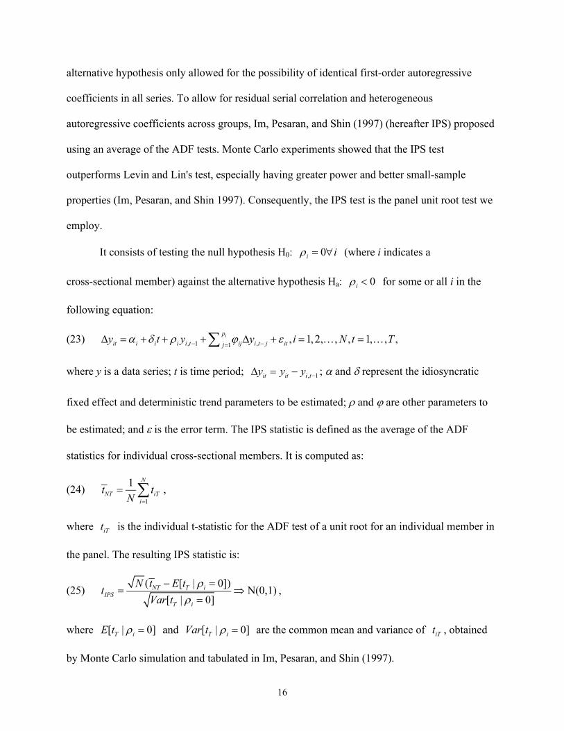
It consists of testing the null hypothesis H0: 0i i (where i indicates a

cross-sectional member) against the alternative hypothesis Ha: 0i for some or all i in the

following equation:

(23) , 1 ,1, 1, 2, , , 1, , ,ip

it i i i i t ij i t j itjy t y y i N t T

where y is a data series; t is time period; , 1it it i ty y y ; and represent the idiosyncratic

fixed effect and deterministic trend parameters to be estimated; and are other parameters to

be estimated; and is the error term. The IPS statistic is defined as the average of the ADF

statistics for individual cross-sectional members. It is computed as:

(24)1

1 N

NT iTi

t tN

,

where iTt is the individual t-statistic for the ADF test of a unit root for an individual member in

the panel. The resulting IPS statistic is:

(25)( [ | 0])

N(0,1)[ | 0]

NT T iIPS

T i

N t E tt

Var t

,

where [ | 0]T iE t and [ | 0]T iVar t are the common mean and variance of iTt , obtained

by Monte Carlo simulation and tabulated in Im, Pesaran, and Shin (1997).

17

As noted by Pedroni (1997) and Kao, Chiang, and Chen (1999) regarding heterogeneous

panels with multiple regressors, it is inappropriate to apply individual unit root tests to judge the

stationarity of estimated residuals from linear combinations of nonstationary variables.

Consequently we pool the time-series and cross-sectional data sets and use Pedroni’s (1999)

panel cointegration tests to test for the existence of a long-run relationship between the

normalized input quantity xj and the right hand-side variables in equations (22).

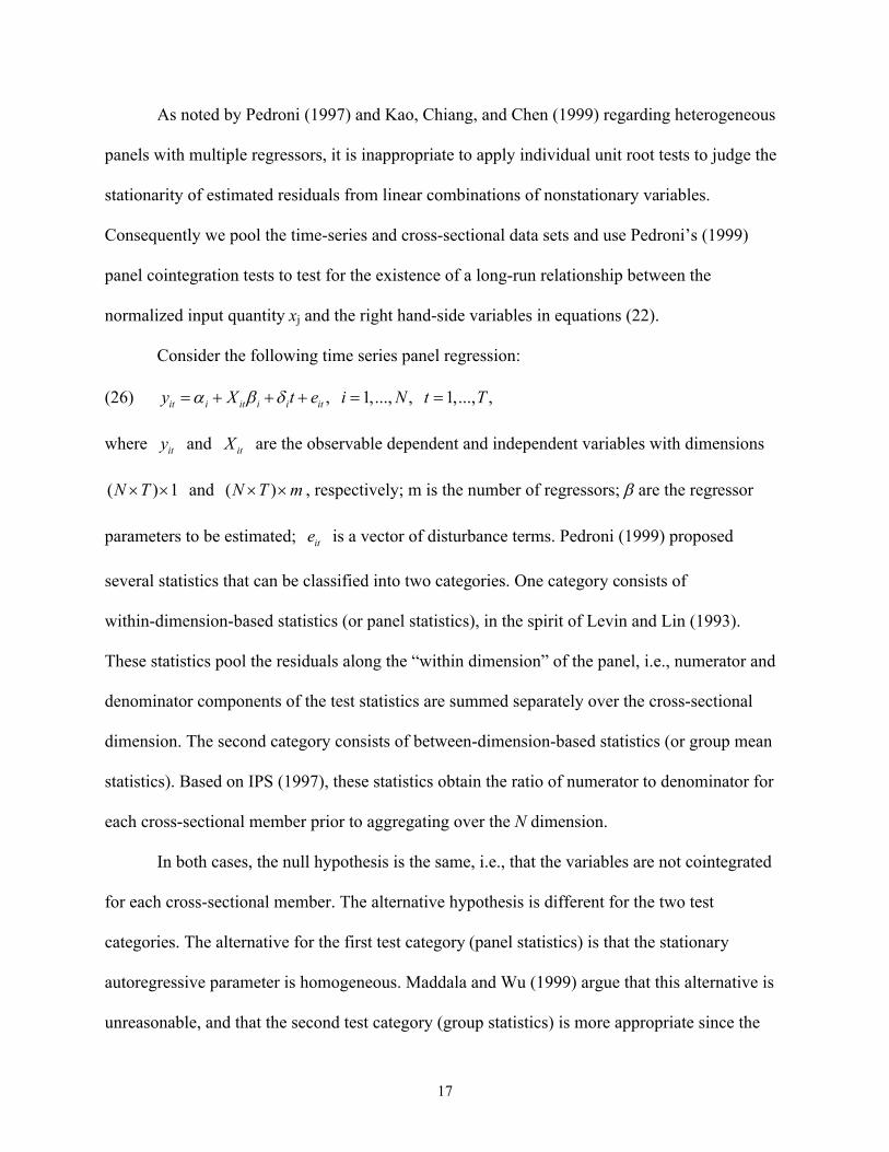
Consider the following time series panel regression:

(26) , 1,..., , 1,..., ,it i it i i ity X t e i N t T

where ity and itX are the observable dependent and independent variables with dimensions

( ) 1N T and ( )N T m , respectively; m is the number of regressors; are the regressor

parameters to be estimated; ite is a vector of disturbance terms. Pedroni (1999) proposed

several statistics that can be classified into two categories. One category consists of

within-dimension-based statistics (or panel statistics), in the spirit of Levin and Lin (1993).

These statistics pool the residuals along the “within dimension” of the panel, i.e., numerator and

denominator components of the test statistics are summed separately over the cross-sectional

dimension. The second category consists of between-dimension-based statistics (or group mean

statistics). Based on IPS (1997), these statistics obtain the ratio of numerator to denominator for

each cross-sectional member prior to aggregating over the N dimension.

In both cases, the null hypothesis is the same, i.e., that the variables are not cointegrated

for each cross-sectional member. The alternative hypothesis is different for the two test

categories. The alternative for the first test category (panel statistics) is that the stationary

autoregressive parameter is homogeneous. Maddala and Wu (1999) argue that this alternative is

unreasonable, and that the second test category (group statistics) is more appropriate since the

18

alternative hypothesis, which permits heterogeneous autoregressive parameters, is less

restrictive.

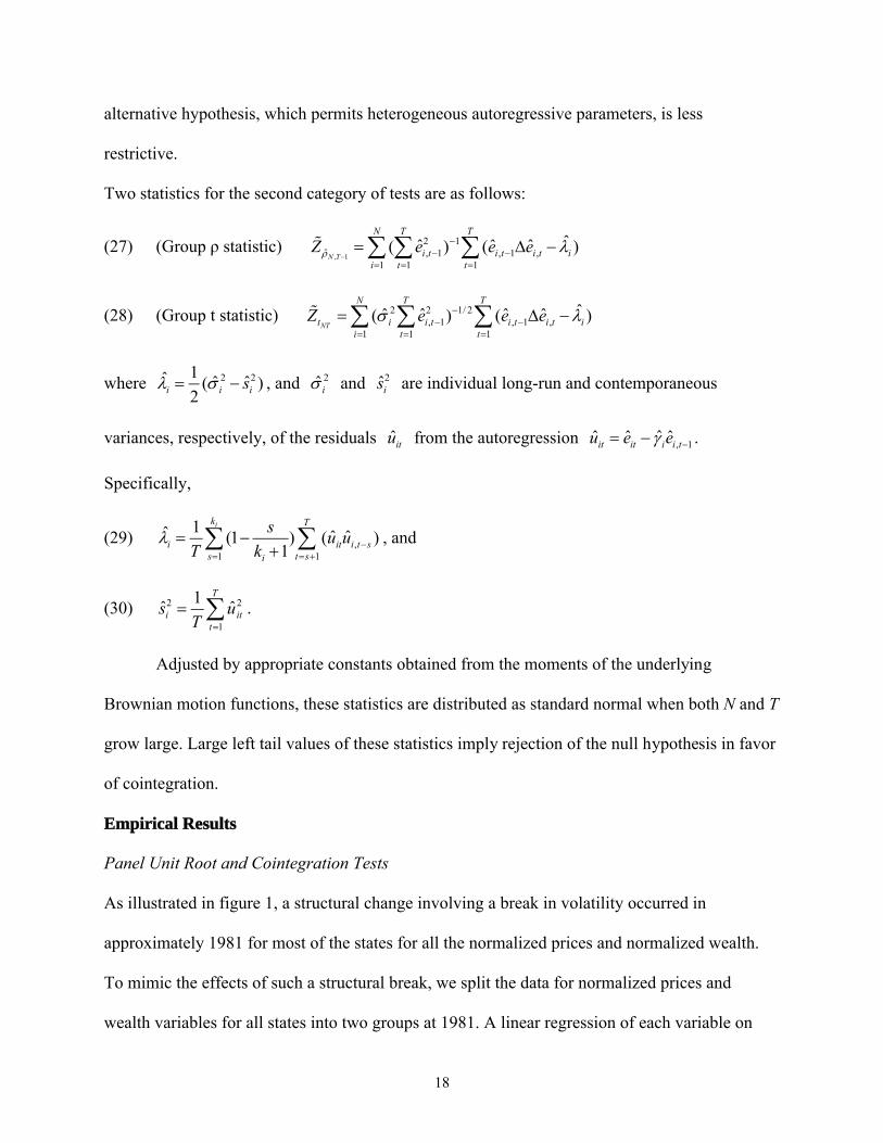
Two statistics for the second category of tests are as follows:

(27) (Group ρ statistic) , 1

2 1ˆ , 1 , 1 ,

1 1 1

ˆˆ ˆ ˆ( ) ( )N T

N T T

i t i t i t ii t t

Z e e e

(28) (Group t statistic) 2 2 1/ 2, 1 , 1 ,

1 1 1

ˆˆ ˆ ˆ ˆ( ) ( )NT

N T T

t i i t i t i t ii t t

Z e e e

where 2 21ˆ ˆ ˆ( )2i i is , and 2ˆi and 2

is are individual long-run and contemporaneous

variances, respectively, of the residuals ˆitu from the autoregression , 1ˆˆ ˆ ˆit it i i tu e e .

Specifically,

(29) ,1 1

1ˆ ˆ ˆ(1 ) ( )1

ik T

i it i t ss t si

su u

T k

, and

(30) 2 2

1

1ˆ ˆ

T

i itt

s uT

.

Adjusted by appropriate constants obtained from the moments of the underlying

Brownian motion functions, these statistics are distributed as standard normal when both N and T

grow large. Large left tail values of these statistics imply rejection of the null hypothesis in favor

of cointegration.

Empirical Results

Panel Unit Root and Cointegration Tests

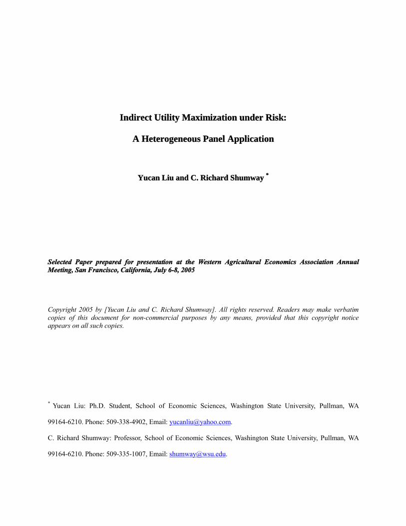
As illustrated in figure 1, a structural change involving a break in volatility occurred in

approximately 1981 for most of the states for all the normalized prices and normalized wealth.

To mimic the effects of such a structural break, we split the data for normalized prices and

wealth variables for all states into two groups at 1981. A linear regression of each variable on

19

year was estimated for each time period, and standard deviations were computed. After dividing

the normalized prices and equity in each time period by the respective standard deviation, the

transformed data were used in the panel tests.

As also illustrated in figure 1, all cross-sectional members in the panel had almost the

same time pattern for prices and equity variables. The implication is that the price series and

equity tended to be driven by some common external disturbance. As recommended by IPS, the

common time effects across states was purged by regressing each normalized price series and

normalized equity on a set of time dummies and using these residuals in the unit root tests. This

approach assumes that the disturbances for each member of the panel can be decomposed into

common disturbances that are shared among all members of the panel and independent

idiosyncratic disturbances that are specific to each member.

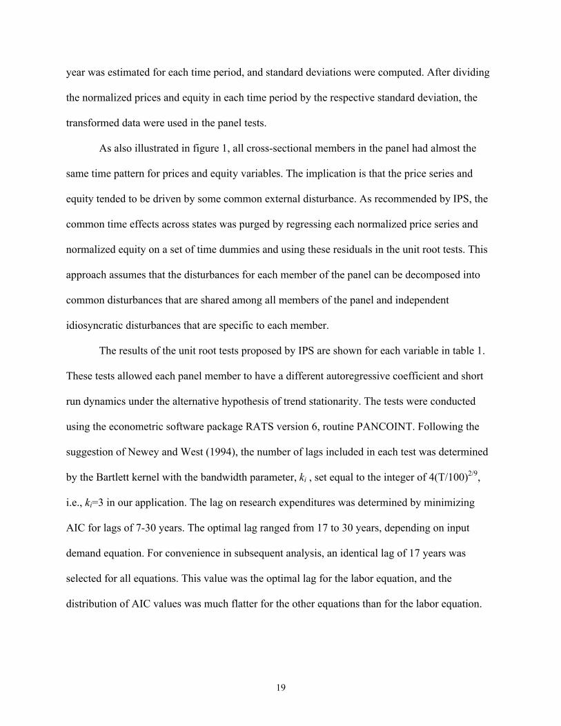
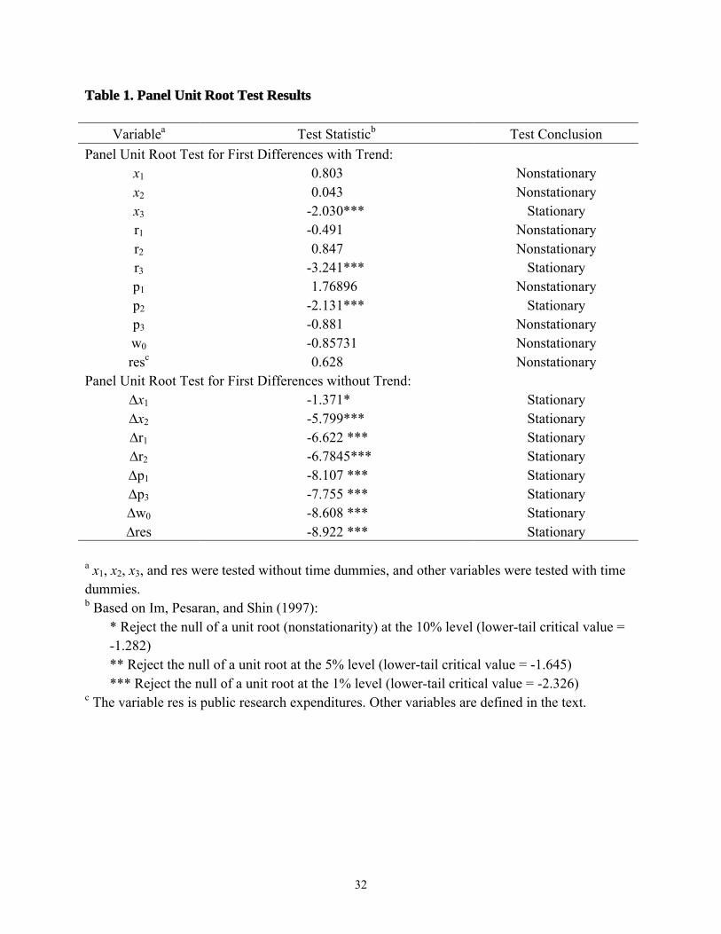
The results of the unit root tests proposed by IPS are shown for each variable in table 1.

These tests allowed each panel member to have a different autoregressive coefficient and short

run dynamics under the alternative hypothesis of trend stationarity. The tests were conducted

using the econometric software package RATS version 6, routine PANCOINT. Following the

suggestion of Newey and West (1994), the number of lags included in each test was determined

by the Bartlett kernel with the bandwidth parameter, ki , set equal to the integer of 4(T/100)2/9,

i.e., ki=3 in our application. The lag on research expenditures was determined by minimizing

AIC for lags of 7-30 years. The optimal lag ranged from 17 to 30 years, depending on input

demand equation. For convenience in subsequent analysis, an identical lag of 17 years was

selected for all equations. This value was the optimal lag for the labor equation, and the

distribution of AIC values was much flatter for the other equations than for the labor equation.

20

The unit root test statistics were distributed as N(0,1) under the null of a unit root with a

one-tailed negative test statistic for the alternative hypothesis.

At the 5% significance level, a unit root was rejected only for the series x3, r3, and p2.

When the other (nonstationary) variables were tested for a unit root in first differences, the

alternative hypothesis was stationarity without a trend since any time trend in levels was

removed by differencing (Canning and Pedroni, 1999). The test statistic for 1st differences was

negative and significant at a 5% level in each variable except for x1. The latter was significant at

a 10% level. Although higher than our prespecified significance level, we accepted x1 as a

stationary series in first differences because it continued to exhibit nonstationarity at the 5% level

even after 4th differencing. Consequently, we conclude that x3, r3, and p2 are stationary, i.e.,

integrated of order zero – I(0), and that all other variables are integrated of order one, I(1).

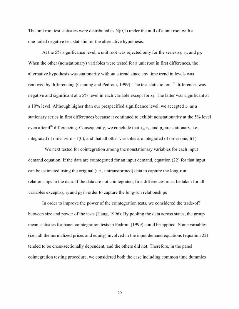
We next tested for cointegration among the nonstationary variables for each input

demand equation. If the data are cointegrated for an input demand, equation (22) for that input

can be estimated using the original (i.e., untransformed) data to capture the long-run

relationships in the data. If the data are not cointegrated, first differences must be taken for all

variables except x3, r3 and p2 in order to capture the long-run relationships

In order to improve the power of the cointegration tests, we considered the trade-off

between size and power of the tests (Haug, 1996). By pooling the data across states, the group

mean statistics for panel cointegration tests in Pedroni (1999) could be applied. Some variables

(i.e., all the normalized prices and equity) involved in the input demand equations (equation 22)

tended to be cross-sectionally dependent, and the others did not. Therefore, in the panel

cointegration testing procedure, we considered both the case including common time dummies

21

(to capture effects that tend to cause individual state variables to move together over time) and

the case without time dummies.

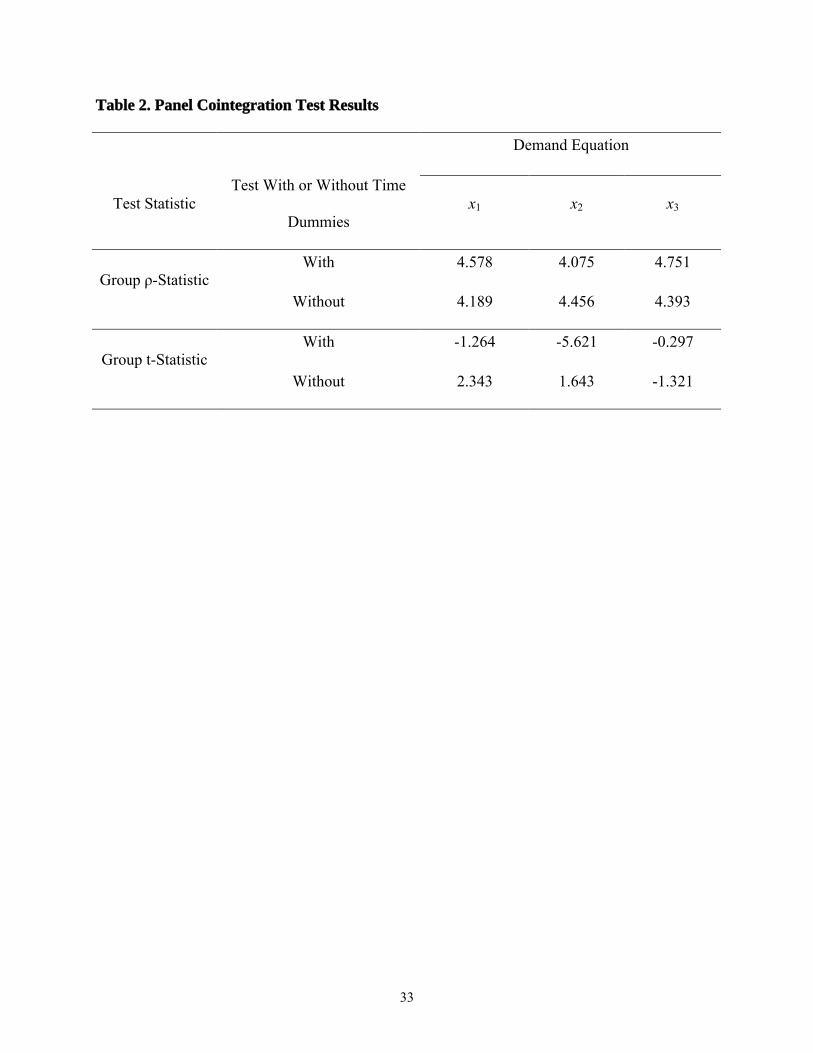
As suggested by Pedroni (1999), the adjustment terms for the panel cointegration tests

were obtained by Monte Carlo simulation on the basis of 10,000 draws of 37 independent

random walks (i.e., the number of regressors exclusive of dummy variables) of length

T=10,000.6 The results of the panel cointegration tests, presented in table 2, show that there is

no evidence of cointegration among the variables for any of the demand equations. Consequently,

the time-series-based input demand equations were estimated using differenced data for all

variables except x3, r3, and p2.

Econometric Model Estimates

For the purpose of comparison, two sets of input demand equations were estimated. They

included (a) the traditional model in which all variables were implicitly assumed to be stationary

and (b) the time-series-based model that accounted for non-rejected time series properties of the

data investigated in last sub-section. In both models, each equation had the same regressors and

no across-equation restrictions were imposed. Consequently, the SUR parameter estimates were

identical to OLS estimates. The SUR estimation procedure was used to permit across-equation

tests to be conducted, as required for proposition 2.

Before estimating the traditional model, we first tested for a 1st-order autoregressive

(AR(1)) process in the error terms for each input demand equation defined in (22). Evidence of

an AR(1) process was found in each equation with Durbin-Watson test statistics of 0.311, 0.317,

and 0.674, respectively, for the materials, capital, and labor input demand equations. Subject to

the assumption that the autoregressive coefficients (rho) within a demand equation were identical

across states, estimates of rho for the three input demand equations were 0.971, 0.923, and 0.870,

22

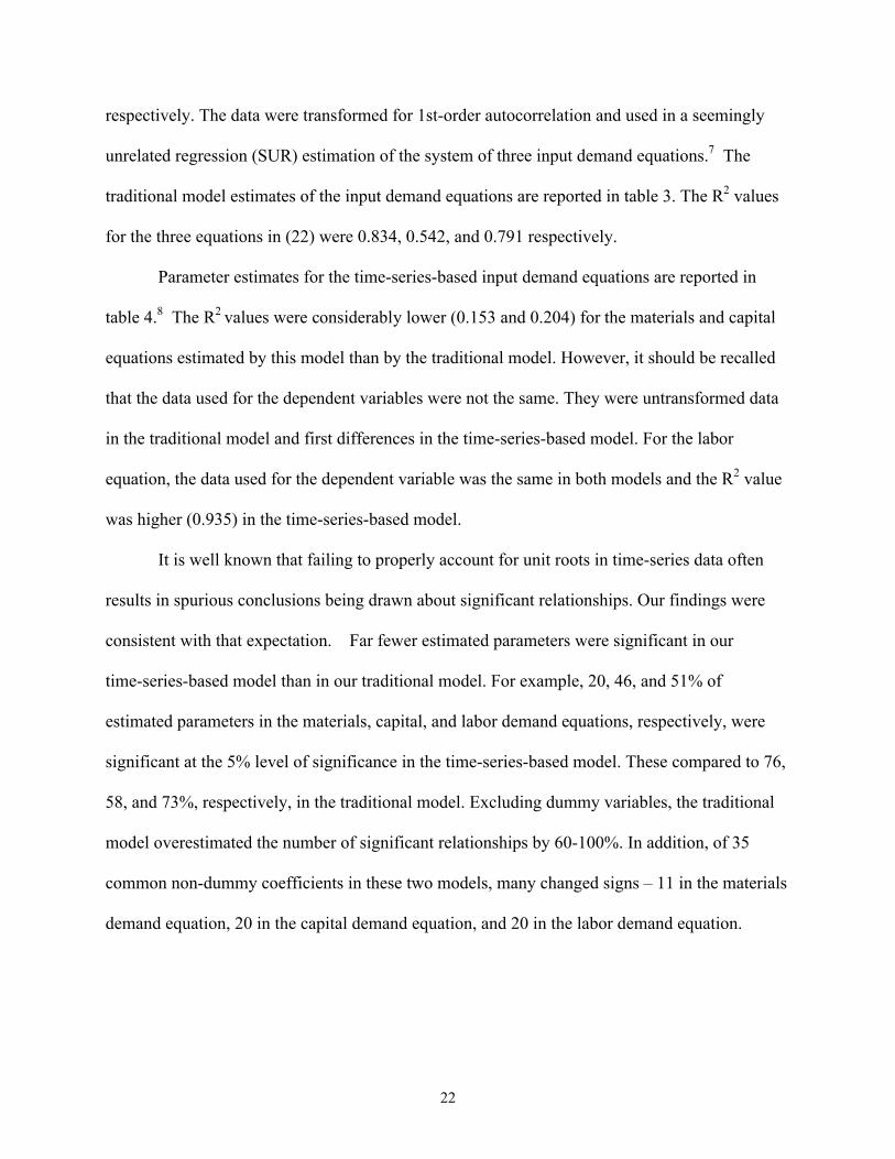
respectively. The data were transformed for 1st-order autocorrelation and used in a seemingly

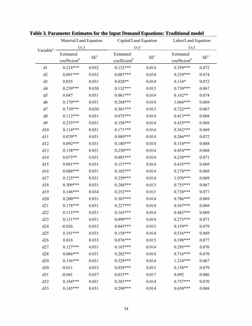
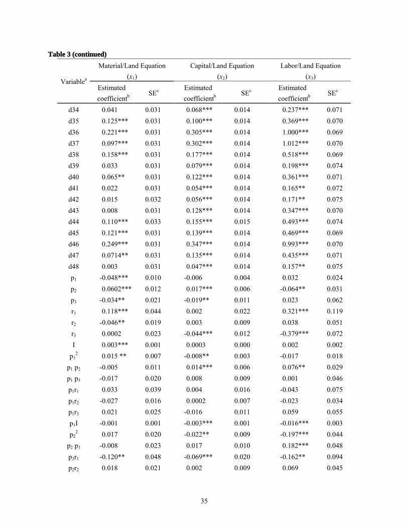
unrelated regression (SUR) estimation of the system of three input demand equations.7 The

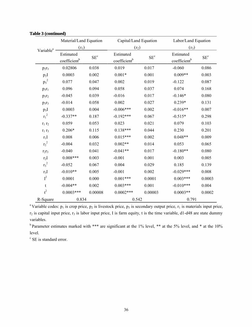
traditional model estimates of the input demand equations are reported in table 3. The R2 values

for the three equations in (22) were 0.834, 0.542, and 0.791 respectively.

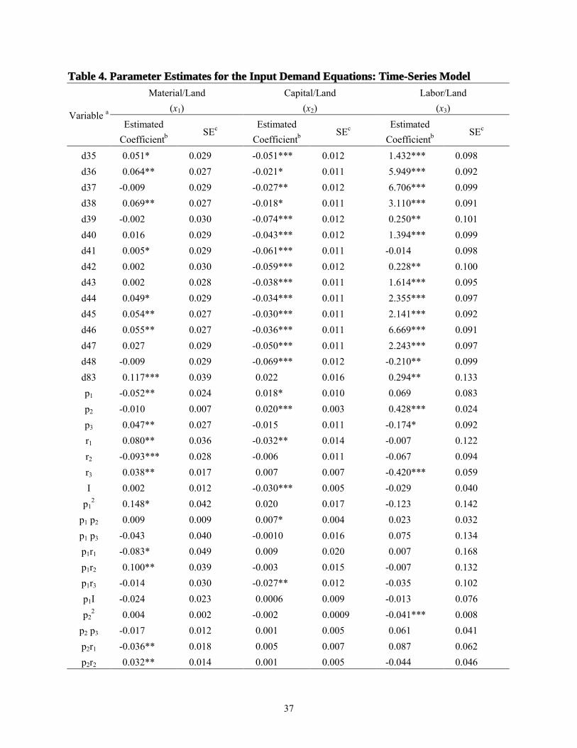
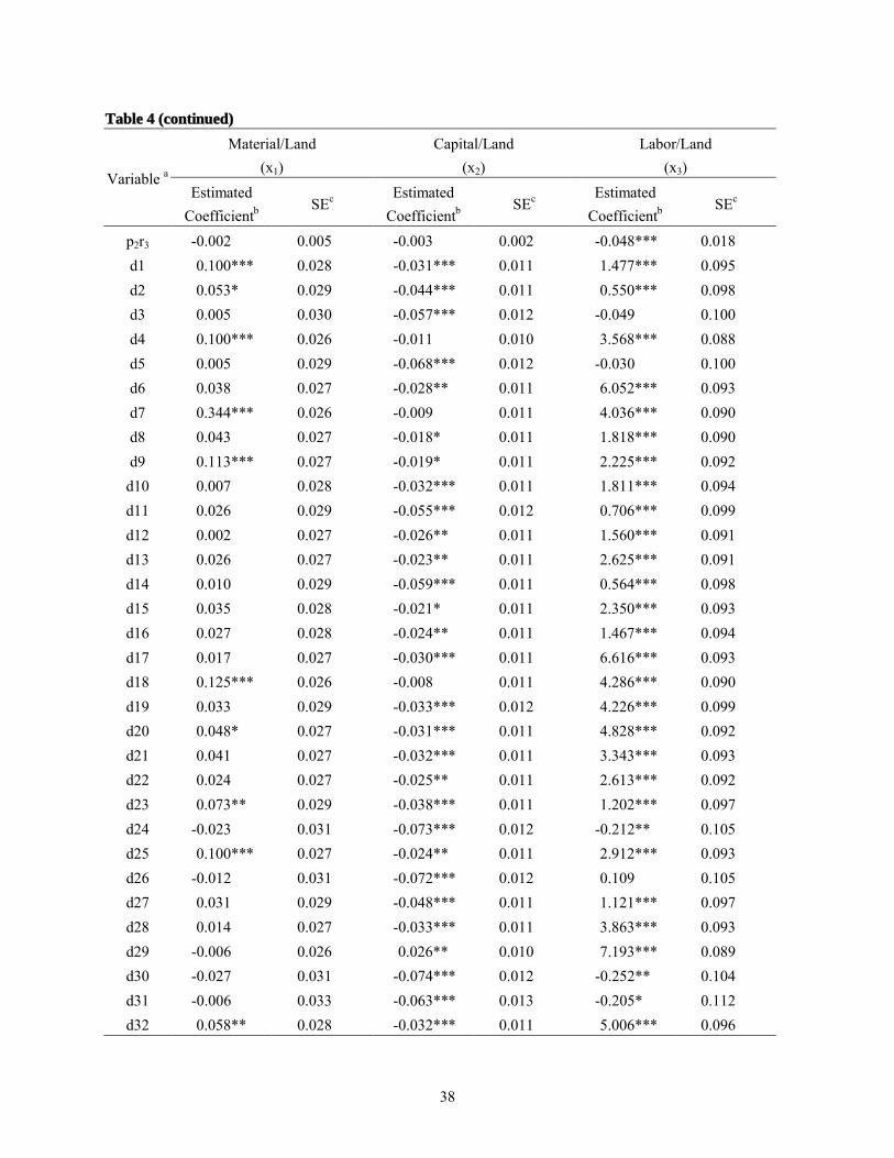
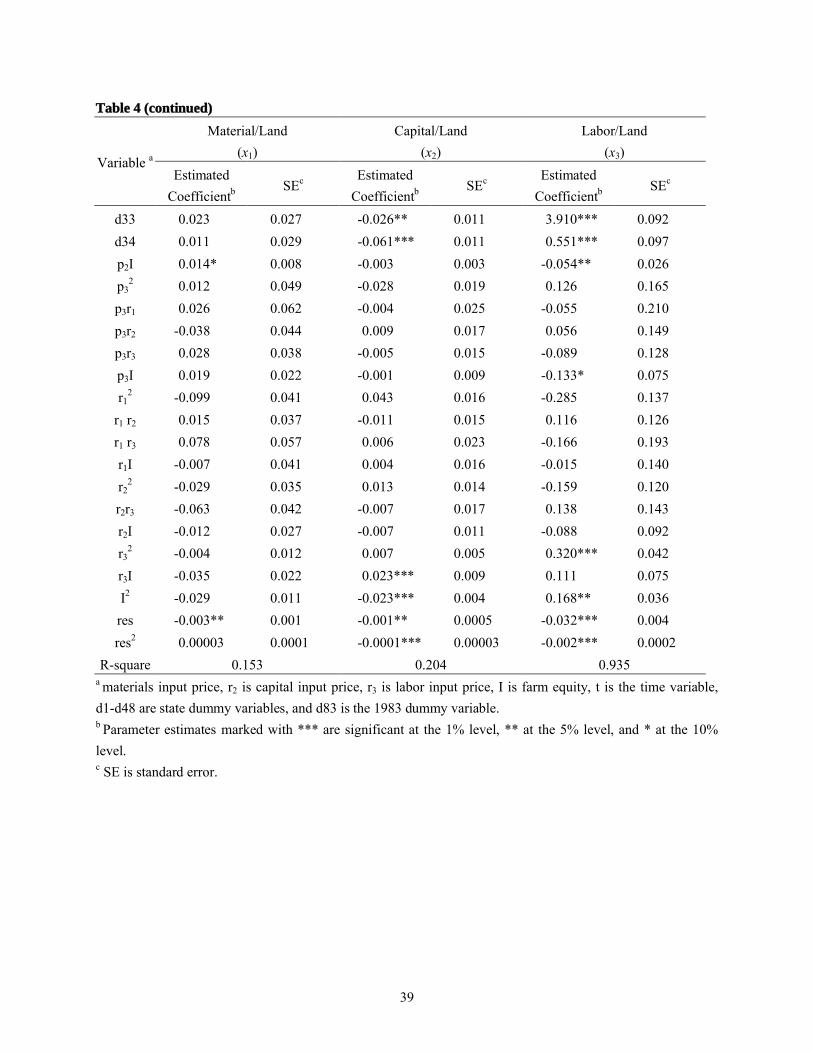
Parameter estimates for the time-series-based input demand equations are reported in

table 4.8 The R2 values were considerably lower (0.153 and 0.204) for the materials and capital

equations estimated by this model than by the traditional model. However, it should be recalled

that the data used for the dependent variables were not the same. They were untransformed data

in the traditional model and first differences in the time-series-based model. For the labor

equation, the data used for the dependent variable was the same in both models and the R2 value

was higher (0.935) in the time-series-based model.

It is well known that failing to properly account for unit roots in time-series data often

results in spurious conclusions being drawn about significant relationships. Our findings were

consistent with that expectation. Far fewer estimated parameters were significant in our

time-series-based model than in our traditional model. For example, 20, 46, and 51% of

estimated parameters in the materials, capital, and labor demand equations, respectively, were

significant at the 5% level of significance in the time-series-based model. These compared to 76,

58, and 73%, respectively, in the traditional model. Excluding dummy variables, the traditional

model overestimated the number of significant relationships by 60-100%. In addition, of 35

common non-dummy coefficients in these two models, many changed signs – 11 in the materials

demand equation, 20 in the capital demand equation, and 20 in the labor demand equation.

23

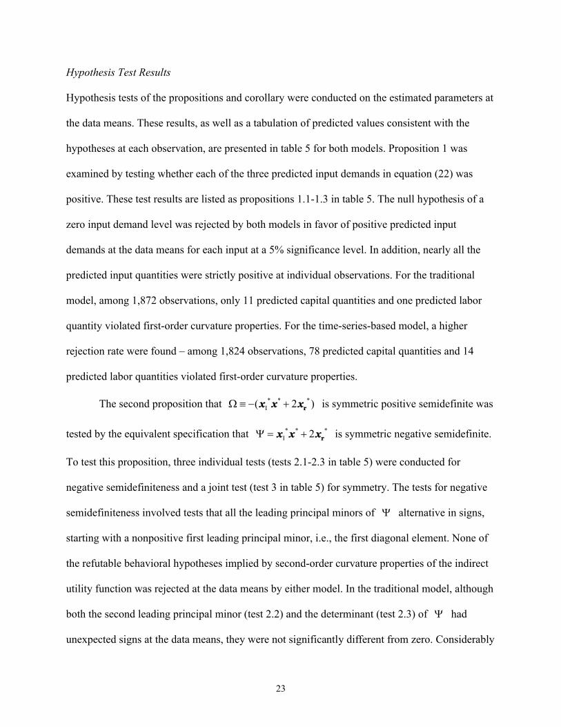
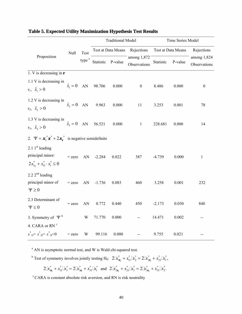
Hypothesis Test Results

Hypothesis tests of the propositions and corollary were conducted on the estimated parameters at

the data means. These results, as well as a tabulation of predicted values consistent with the

hypotheses at each observation, are presented in table 5 for both models. Proposition 1 was

examined by testing whether each of the three predicted input demands in equation (22) was

positive. These test results are listed as propositions 1.1-1.3 in table 5. The null hypothesis of a

zero input demand level was rejected by both models in favor of positive predicted input

demands at the data means for each input at a 5% significance level. In addition, nearly all the

predicted input quantities were strictly positive at individual observations. For the traditional

model, among 1,872 observations, only 11 predicted capital quantities and one predicted labor

quantity violated first-order curvature properties. For the time-series-based model, a higher

rejection rate were found – among 1,824 observations, 78 predicted capital quantities and 14

predicted labor quantities violated first-order curvature properties.

The second proposition that * * *I( 2 ) rх х х is symmetric positive semidefinite was

tested by the equivalent specification that * * *I 2 rх х х is symmetric negative semidefinite.

To test this proposition, three individual tests (tests 2.1-2.3 in table 5) were conducted for

negative semidefiniteness and a joint test (test 3 in table 5) for symmetry. The tests for negative

semidefiniteness involved tests that all the leading principal minors of alternative in signs,

starting with a nonpositive first leading principal minor, i.e., the first diagonal element. None of

the refutable behavioral hypotheses implied by second-order curvature properties of the indirect

utility function was rejected at the data means by either model. In the traditional model, although

both the second leading principal minor (test 2.2) and the determinant (test 2.3) of had

unexpected signs at the data means, they were not significantly different from zero. Considerably

24

more evidence of second-order curvature violations than of first-order curvature violations at

individual observations than of first-order condition violations. Except for test 2.3 with the

time-series-based model, individual violations didn’t exceed 25% of the observations.

The test results for symmetry of are presented in test 3 in table 5. The three

symmetric restrictions were rejected at the 5% significance level by the joint test conducted at

data means in both models. Thus, the hypothesis implied by proposition 2 that is symmetric

positive semidefinite is statistically rejected at this data point. Whether rejection of symmetry

constitutes a rejection of the hypothesis that the collection of firms in each state act as though

they were a single expected utility-maximizing firm, or whether it simply implies that the

indirect utility function is not twice continuously differentiable at the data means is ambiguous

from these test results. Unfortunately, we are unable to resolve the ambiguity in this article.

Decision making consistent with constant absolute risk aversion or risk neutrality implies

three restrictions on input demand responses. The result (test 4 in table 5) indicates that these

restrictions were rejected by the joint test at the data means at the 5% significance level in both

models.

Our results using state-level aggregates were similar in a number of respects to Saha and

Shumway’s (1998) findings about output price risk for Kansans wheat farmers. However, we

found less support in the aggregate data than they found in the firm-level data for symmetry of

the indirect utility function. Our conclusions about first-order curvature properties and the nature

of producers’ risk preference were the same as theirs. The extant literature has not reached a

consensus regarding the nature of farmers’ risk preferences (Goodwin and Mishra, 2002), but a

few have found empirical support for the hypothesis of constant absolute risk aversion (CARA).

25

Among those are the work of Park and Antonovitz (1992a, 1992b) who failed to reject CARA

for California feedlots.

Conclusions

This study has extended the Saha and Shumway (1998) model of a competitive firm operating

under output price risk to a firm operating under both output price and output quantity risk. One

important theoretical contribution to the previous literature is that the refutable propositions

implied by the indirect utility function are shown to hold without one of the previously

maintained hypotheses. Therefore, the only conditions required for the propositions to hold are:

(a) random wealth can be structured as three parts – a nonrandom part of profit, a random part of

profit, and nonrandom initial wealth, and (b) there exists an optimal input vector that maximizes

the expected utility function. Both are common assumptions in the firm theory under uncertainty.

Without requiring the previously imposed assumption that the expectation of the random part of

profit is zero, the propositions can be empirically applied to varied market structures by

permitting tests when there is a nonzero correlation between the error terms of random output

price and random output quantity.

Moreover, a set of testable hypotheses associated with input responses under multiple

sources of risk were derived from these propositions, and empirically tested for aggregates of

firms operating under both output price and output quantity risk. This is the first study using an

aggregate state-level panel data set to empirically test for utility-maximizing behavior by

considering each aggregate as though it were an expected utility-maximizing firm. Aggregate

agricultural production data for these states have previously been found to approximate

nonparametric conditions for consistent behavior with this hypothesis.

26

To avoid the possibility of spurious estimation from statistical estimation using

nonstationary data, we examined the time series properties of the data. The data were tested both

for nonstationarity and cointegration using recent developments in time-series econometrics, i.e.,

Im, Pesaran, and Shin’s panel unit root tests and Pedroni’s panel cointegration tests. Most of the

data series were found to be nonstationary but none of the demand equations exhibited evidence

of cointegration among nonstationary variables. Two models were developed and used for

comparison purposes to test the expected utility maximization hypotheses – a traditional model

that implicitly assumed stationary data and a model based on nonrejected time series properties

of the data.

In both models, parametric results showed that the behavioral postulates implied by the

first-order curvature properties of the indirect utility function could not be rejected at the data

means, and the data at nearly all individual observations were consistent with these properties.

The second-order curvature properties were also not rejected at the data means, but a larger

portion of the observations were inconsistent with the hypotheses. The symmetry property

implied by a twice continuously differentiable indirect utility function was soundly rejected at

the data means by both models. The empirical evidence from both models also failed to support

ad hoc risk preference assumptions of either risk neutrality or constant absolute risk aversion.

27

Footnotes

1 See Banerjee (1999), Baltagi and Kao (1999), and Phillips and Moon (1999) for surveys of the recent theoretical

literature on panel unit root tests and panel cointegration tests.

2 Exceptions are Bandiera et al. (2000), McCoskey and Kao (1999), and Sarantis and Stewart (2001).

3 The following notation is used throughout this article: hx denotes the partial derivative of h(∙) with respect to x, hxy

represents the Hessian matrix whose ijth element is 2/

i jh x y , where h(∙) is a real-value function of vectors x and y.

4 The theory of the expected utility maximization applies to the individual, in this case the individual firm. Although

tests of utility maximization have not been reported for state-level data, Lim and Shumway (1992) failed to reject

the hypothesis that each of the states acted as though they were profit-maximizing firms. They used nonparametric

testing procedures on annual data for the period 1956-1982, which overlaps with the first 23 years of our data

period.

5 Significant (5% level) groupwise heteroskadasticity was still found in the scaled data.

6 Pedroni (1999) tabulated the adjustment terms for a maximum of seven regressors.

7 Although evidence was found that significant heteroskedasticity still remained across states, we were unable to

transform the data to remove cross-sectional heteroskedasticity because we had more cross-sectional units than time

periods.

8 An additional dummy variable was included in each input demand equation in the time-series-based model for the

production year 1983 to pick up the effects of the PIK program.

References

Adrangi, B. and K. Raffiee. 1999. “On Total Price Uncertainty and the Behavior of aCompetitive Firm.” American Economist 43:59-65.

Antonovitz, F. and T. Roe. 1986. “Effects of Expected Cash and Futures Prices on Hedging and Production.” The Journal of Futures Markets 6:187-205.

Arrow, K.J. 1965. Aspects of the Theory of Risk Bearing. Helsinki: Academic Publishers.

Ball, V.E. 2002. “U.S. and State-Level Agricultural Data Sets.” Unpublished, Washington: U.S. Department of Agriculture, ERS.

Ball, V.E., F.M. Gollop, A. Kelly-Hawke, and G.P. Swinand. 1999. “Patterns of State Productivity Growth in the U.S. Farm Sector: Linking State and Aggregate Models.” American Journal of Agricultural Economics 81:164-79.

Baltagi, B.H. and C. Kao. 2000. “Nonstationary Panels, Cointegration in Panels and Dynamic Panels: A Survey.” Advances in Econometrics 15:7-51.

Bandiera, O., G. Caprio, P. Honohan, and F. Schiantarelli. “Does Financial Reform Raise or Reduce Saving?” Review of Economics and Statistics 82 (2000): 239-263.

Banerjee, A. 1999. “Panel Data Unit Roots and Cointegration: an Overview.” Oxford Bulletin of Economics and Statistics 61:607-29.

Batra, R. N., and A. Ullah. “Competitive Firm and the Theory of Input Demand under Price Uncertainty.” The Journal of Political Economy 82 (May-Jun1974): 537-548.

Canning, D. and P. Pedroni. “Infrastructure and Long Run Economic Growth.” CAER II Discussion Paper No. 57, Harvard Institute for International Development, 1999.

Chavas, J.P. and T.L. Cox. 1992. “A Nonparametric Analysis of the Influence of Research on Agricultural Productivity.” American Journal of Agricultural Economics 74:583-91.

Chavas, J.P. and R. Pope. 1985. “Price Uncertainty and Competitive Firm Behavior: Testable Hypotheses from Expected Utility Maximization.” Journal of Economics and Business37:223-35.

Chavas, J.P. and M.T. Holt. 1990. “Acreage Decisions Under Risk: The Case of Corn and Soybeans.” American Journal of Agricultural Economics 72:529-38.

_____. 1996 “Economic Behavior Under Uncertainty: A Joint Analysis of Risk Preferences and Technology.” The Review of Economics and Statistics 78:329-35.

Chavas, J.P. and R. Pope. 1985. “Price Uncertainty and Competitive Firm Behavior: Testable Hypotheses from Expected Utility Maximization.” Journal of Economics and Business37:223-35.

29

Dalal, A.J. 1990. “Symmetry restrictions in the analysis of the competitive firm under price uncertainty.” International Economic Review 31:207-211.

_____. 1994. “Econometric Tests of Firm Decision Making under Uncertainty — Optimal Output and Hedging: Comment.” Southern Economic Journal 61:213-17.

Engle, R.F. and C.W.J. Granger. 1987. “Co-integration and Error Correction: Representation, Estimation, and Testing.” Econometrica 55:251-76.

Feder, B. 1977. “The Impact of Uncertainty in a Class of Objective Functions.” Journal of Economic Theory 16:504-12.

Goodwin, B.K. and A.K. Mishra. 2002. “Are ‘Decoupled’ Farm Program Payments Really Decoupled? An Empirical Evaluation.” Working Paper, Columbus: Department of Agricultural, Environmental, and Development Economics, Ohio State University.

Haug, A.A. 1996 “Tests for Cointegration. A Monte Carlo Comparison” Journal of Econometrics 71:89-115.

Harris, R.D.F. and E. Tzavalis. 1999. “Inference for Unit Roots in Dynamic Panels where the Time Dimension is Fixed.” Journal of Econometrics 91:201-26.

Huffman, W.E. 2002. “Agricultural Research and Extension Expenditure Data.” Unpublished, Ames: Department of Economics, Iowa State University.

Im, K.S., M.H. Pesaran, and Y. Shin. 1997. “Testing for Unit Roots in Heterogeneous Panels.”Working Paper: Cambridge: University of Cambridge, Department of Applied Economics.

Kao, C., M. Chiang, and B. Chen. 1999. “International R&D Spillovers: an Application of Estimation and Inference in Panel Cointegration.” Oxford Bulletin of Economics and Statistics 61:693-711.

Kumbhakar, S.C. 2002. “Specification and Estimation of Production Risk, Risk Preferences and Technical Efficiency.” American Journal of Agricultural Economics 84:8-22.

Kumbhakar, S.C. and R. Tveteras. 2003. “Risk Preferences, Production Risk and Firm Heterogeneity.” Scandinavian Journal of Economics 105:275-93.

Levin, A. and C. Lin. 1993. “Unit Root Tests in Panel Data: Asymptotic and Finite-Sample Properties.” Working Paper, San Diego: University of California.

Lien, G. and J.B. Hardaker. 2001. “Whole-farm Planning Under Uncertainty: Impacts of Subsidy Scheme and Utility Function on Portfolio Choice in Norwegian Agriculture.” European Review of Agricultural Economics 28:17-36.

30

Lim, H. and C.R. Shumway. 1992. “Profit Maximization, Returns to Scale, and Measurement Error.” Review of Economics and Statistics 74:430-38.

Love, H. A. and S.T. Buccola. 1991. “Joint Risk Preference-Technology Estimation with a Primal System.” American Journal of Agricultural Economics 73:765-74.

Maddala, G.S. and S. Wu. 1999. “A Comparative Study of Unit Root Tests with Panel Data and a New Simple Test.” Oxford Bulletin of Economics and Statistics 61:631-52.

McCoskey, S. and C. Kao. 1999. “Testing the Stability of a Production Function with Urbanization as a Shift Factor.” Oxford Bulletin of Economics and Statistics 61:671-90.

Meyer, D.J. and J. Meyer. 1998. “Determining Risk Attitudes for Agricultural Producers.” Working Paper, Lansing: Department of Economics, Michigan State University.

Newey, W. and K. West. 1994. “Autocovariance Lag Selection in Covariance Matrix Estimation.” Review of Economic Studies 61:631-653.

Pardey, P.G. and B. Craig. 1989. “Causal Relationships between Public Sector Agricultural Research Expenditures and Output.” American Journal of Agricultural Economics71:9-19.

Paris, Q. 1988. “Long-run Comparative Statics under Output and Land Price Uncertainty.” American Journal of Agricultural Economics 70:133-41.

Park, T.A. and F. Antonovitz. 1992a. “Testable Hypotheses of the Competitive Firm Using Hedging to Manage Price Risk.” Journal of Economics and Business 44:169-85.

Park, T.A. and F. Antonovitz. 1992b. “Economic Tests of Firm Decision Making under Uncertainty: Optimal Output and Hedging Decisions.” Southern Economic Journal58:593-609.

Pedroni, P. 1999. “Critical Values for Cointegration Tests in Heterogeneous Panels withMultiple Regressors”, Oxford Bulletin of Economics and Statistics 61:653-78.

_____. 1997. “Panel Cointegration; Asymptotic and Finite Sample Properties of Pooled Time Series Tests, With an Application to the PPP Hypothesis: New Results.” Working Paper, Bloomington: Indiana University.

Phillips, P.C.B. 1986. “Understanding Spurious Regressions in Econometrics.” Journal of Econometrics 33:311-40.

Phillips, P.C.B. and H.R. Moon. 1999. “Nonstationary Panel Data Analysis: An Overview of Some Recent Developments.” Working Paper, New Haven: Cowles Foundation, Yale University.

Pope, R.D. 1980. “The Generalized Envelope Theorem and Price Uncertainty.” International Economic Review 21:75-86.

31

Pratt, J.W. 1964. “Risk Aversion in the Small and in the Large.” Econometrica 32:122-36.

Quah, D. 1992. “International Patterns of Growth: I, Persistence in Cross-Country Disparities.”Unpublished Manuscript, Oxford: London School of Economics.

_____. 1994. “Exploiting Cross-Section Variations for Unit Root Inference in Dynamic Data.”Economics Letters 44:9-19.

Roosen, J. and D.A. Hennessy. 2003. “Tests for the Role of Risk Aversion on Input Use.”American Journal of Agricultural Economics 85:30-43.

Saha, A. and C.R. Shumway. 1998. “Refutable Implications of the Firm Model under Risk.”Applied Economics 30:441-48.

Saha, A., C.R. Shumway, and H. Talpaz. 1994. “ Joint Estimation of Risk Preference Structure and Technology Using Expo-Power Utility.” American Journal of Agricultural Economics 76:173-84.

Sandmo A. 1971. “On the Theory of the Competitive Firm under Price Uncertainty.” The American Economic Review 61:65-73.

Sarantis, N. and C. Stewart. 2001. “Saving Behaviour in OECD Countries: Evidence from Panel Cointegration Tests.” The Manchester School Supplement pp. 22-41.

Satyanarayan, S. 1999. “Econometric Tests of Firm Decision Making under Dual Sources of Uncertainty.” Journal of Economics and Business 51:315-25.

U.S. Department of Agriculture/Economic Research Service. 1960-1999. Farm Balance Sheet.Annual Series, http://www.ers.usda.gov/data/farmbalancesheet/fbsdmu.htm.

32

Table 1. Panel Unit Root Test Results

Variablea Test Statisticb Test Conclusion

Panel Unit Root Test for First Differences with Trend:x1 0.803 Nonstationaryx2 0.043 Nonstationaryx3 -2.030*** Stationaryr1 -0.491 Nonstationaryr2 0.847 Nonstationaryr3 -3.241*** Stationaryp1 1.76896 Nonstationaryp2 -2.131*** Stationaryp3 -0.881 Nonstationaryw0 -0.85731 Nonstationaryresc 0.628 Nonstationary

Panel Unit Root Test for First Differences without Trend:x1 -1.371* Stationaryx2 -5.799*** Stationaryr1 -6.622 *** Stationaryr2 -6.7845*** Stationaryp1 -8.107 *** Stationaryp3 -7.755 *** Stationaryw0 -8.608 *** Stationaryres -8.922 *** Stationary

a x1, x2, x3, and res were tested without time dummies, and other variables were tested with time dummies.b Based on Im, Pesaran, and Shin (1997):

* Reject the null of a unit root (nonstationarity) at the 10% level (lower-tail critical value = -1.282)** Reject the null of a unit root at the 5% level (lower-tail critical value = -1.645)*** Reject the null of a unit root at the 1% level (lower-tail critical value = -2.326)

c The variable res is public research expenditures. Other variables are defined in the text.

33

Table 2. Panel Cointegration Test Results

Demand Equation

Test StatisticTest With or Without Time

Dummiesx1 x2 x3

With 4.578 4.075 4.751Group ρ-Statistic

Without 4.189 4.456 4.393

With -1.264 -5.621 -0.297Group t-Statistic

Without 2.343 1.643 -1.321

34

Table 3. Parameter Estimates for the Input Demand Equations: Traditional model

Material/Land Equation

(x1)

Capital/Land Equation

(x2)

Labor/Land Equation

(x3)Variablea

Estimated

coefficientbSEc Estimated

coefficientbSEc Estimated

coefficientbSEc

d1 0.218*** 0.032 0.132*** 0.014 0.359*** 0.072

d2 0.091*** 0.032 0.087*** 0.014 0.239*** 0.074

d3 0.035 0.031 0.028** 0.014 0.134* 0.072

d4 0.239*** 0.030 0.132*** 0.013 0.730*** 0.067

d5 0.047 0.031 0.061*** 0.014 0.162** 0.074

d6 0.170*** 0.031 0.284*** 0.014 1.068*** 0.069

d7 0.739*** 0.030 0.301*** 0.013 0.722*** 0.067

d8 0.112*** 0.031 0.075*** 0.014 0.413*** 0.068

d9 0.235*** 0.031 0.156*** 0.014 0.435*** 0.069

d10 0.114*** 0.031 0.171*** 0.014 0.362*** 0.069

d11 0.070** 0.031 0.089*** 0.014 0.266*** 0.072

d12 0.092*** 0.031 0.180*** 0.014 0.310*** 0.068

d13 0.138*** 0.031 0.230*** 0.014 0.454*** 0.068

d14 0.075** 0.031 0.093*** 0.014 0.230*** 0.071

d15 0.091*** 0.031 0.157*** 0.014 0.435*** 0.069

d16 0.086*** 0.031 0.102*** 0.014 0.278*** 0.069

d17 0.125*** 0.031 0.259*** 0.014 1.070*** 0.069

d18 0.309*** 0.031 0.288*** 0.013 0.755*** 0.067

d19 0.146*** 0.034 0.252*** 0.015 0.730*** 0.077

d20 0.200*** 0.031 0.307*** 0.014 0.786*** 0.069

d21 0.178*** 0.031 0.227*** 0.014 0.567*** 0.069

d22 0.115*** 0.031 0.165*** 0.014 0.465*** 0.069

d23 0.131*** 0.031 0.099*** 0.014 0.273*** 0.071

d24 -0.026 0.033 0.043*** 0.015 0.159** 0.079

d25 0.191*** 0.031 0.158*** 0.014 0.516*** 0.069

d26 0.018 0.033 0.076*** 0.015 0.198*** 0.077

d27 0.127*** 0.031 0.107*** 0.014 0.295*** 0.070

d28 0.086*** 0.031 0.202*** 0.014 0.716*** 0.070

d29 0.156*** 0.031 0.529*** 0.014 1.234*** 0.067

d30 -0.011 0.033 0.039*** 0.015 0.158** 0.079

d31 -0.041 0.037 0.033** 0.017 0.092 0.086

d32 0.184*** 0.031 0.283*** 0.014 0.757*** 0.070

d33 0.145*** 0.031 0.290*** 0.014 0.650*** 0.068

35

Table 3 (continued)

Material/Land Equation

(x1)

Capital/Land Equation

(x2)

Labor/Land Equation

(x3)Variablea

Estimated

coefficientbSEc Estimated

coefficientbSEc Estimated

coefficientbSEc

d34 0.041 0.031 0.068*** 0.014 0.237*** 0.071

d35 0.125*** 0.031 0.100*** 0.014 0.369*** 0.070

d36 0.221*** 0.031 0.305*** 0.014 1.000*** 0.069

d37 0.097*** 0.031 0.302*** 0.014 1.012*** 0.070

d38 0.158*** 0.031 0.177*** 0.014 0.518*** 0.069

d39 0.033 0.031 0.079*** 0.014 0.198*** 0.074

d40 0.065** 0.031 0.122*** 0.014 0.361*** 0.071

d41 0.022 0.031 0.054*** 0.014 0.165** 0.072

d42 0.015 0.032 0.056*** 0.014 0.171** 0.075

d43 0.008 0.031 0.128*** 0.014 0.347*** 0.070

d44 0.110*** 0.033 0.155*** 0.015 0.493*** 0.074

d45 0.121*** 0.031 0.139*** 0.014 0.469*** 0.069

d46 0.249*** 0.031 0.347*** 0.014 0.993*** 0.070

d47 0.0714** 0.031 0.135*** 0.014 0.435*** 0.071

d48 0.003 0.031 0.047*** 0.014 0.157** 0.075

p1 -0.048*** 0.010 -0.006 0.004 0.032 0.024

p2 0.0602*** 0.012 0.017*** 0.006 -0.064** 0.031

p3 -0.034** 0.021 -0.019** 0.011 0.023 0.062

r1 0.118*** 0.044 0.002 0.022 0.321*** 0.119

r2 -0.046** 0.019 0.003 0.009 0.038 0.051

r3 0.0002 0.023 -0.044*** 0.012 -0.379*** 0.072

I 0.003*** 0.001 0.0003 0.000 0.002 0.002

p12 0.015 ** 0.007 -0.008** 0.003 -0.017 0.018

p1 p2 -0.005 0.011 0.014*** 0.006 0.076** 0.029

p1 p3 -0.017 0.020 0.008 0.009 0.001 0.046

p1r1 0.033 0.039 0.004 0.016 -0.043 0.075

p1r2 -0.027 0.016 0.0002 0.007 -0.023 0.034

p1r3 0.021 0.025 -0.016 0.011 0.059 0.055

p1I -0.001 0.001 -0.003*** 0.001 -0.016*** 0.003

p22 0.017 0.020 -0.022** 0.009 -0.197*** 0.044

p2 p3 -0.008 0.023 0.017 0.010 0.182*** 0.048

p2r1 -0.120** 0.048 -0.069*** 0.020 -0.162** 0.094

p2r2 0.018 0.021 0.002 0.009 0.069 0.045

36

Table 3 (continued)

Material/Land Equation

(x1)

Capital/Land Equation

(x2)

Labor/Land Equation

(x3)Variablea

Estimated

coefficientbSEc Estimated

coefficientbSEc Estimated

coefficientbSEc

p2r3 0.02806 0.038 0.019 0.017 -0.060 0.086

p2I 0.0003 0.002 0.001* 0.001 0.009** 0.003

p32 0.077 0.047 0.002 0.019 -0.122 0.087

p3r1 0.096 0.094 0.058 0.037 0.074 0.168

p3r2 -0.045 0.039 -0.016 0.017 -0.146* 0.080

p3r3 -0.014 0.058 0.002 0.027 0.239* 0.131

p3I 0.0003 0.004 -0.006*** 0.002 -0.016** 0.007

r12 -0.337** 0.187 -0.192*** 0.067 -0.515* 0.298

r1 r2 0.059 0.053 0.023 0.021 0.079 0.103

r1 r3 0.206* 0.115 0.138*** 0.044 0.230 0.201

r1I 0.008 0.006 0.015*** 0.002 0.048** 0.009

r22 -0.004 0.032 0.002** 0.014 0.053 0.065

r2r3 -0.040 0.041 -0.041** 0.017 -0.180** 0.080

r2I 0.008*** 0.003 -0.001 0.001 0.003 0.005

r32 -0.052 0.067 0.004 0.029 0.185 0.139

r3I -0.010** 0.005 -0.001 0.002 -0.029*** 0.008

I2 0.0001 0.000 0.001*** 0.0001 0.003*** 0.0003

t -0.004** 0.002 0.003*** 0.001 -0.010*** 0.004

t2 0.0003*** 0.00008 0.0002*** 0.00003 0.0003** 0.0002

R-Square 0.834 0.542 0.791a Variable codes: p1 is crop price, p2 is livestock price, p3 is secondary output price, r1 is materials input price,

r2 is capital input price, r3 is labor input price, I is farm equity, t is the time variable, d1-d48 are state dummy

variables.b Parameter estimates marked with *** are significant at the 1% level, ** at the 5% level, and * at the 10%

level.c SE is standard error.

37

Table 4. Parameter Estimates for the Input Demand Equations: Time-Series Model

Material/Land

(x1)

Capital/Land

(x2)

Labor/Land

(x3)Variable a

Estimated

CoefficientbSEc Estimated

CoefficientbSEc Estimated

CoefficientbSEc

d35 0.051* 0.029 -0.051*** 0.012 1.432*** 0.098

d36 0.064** 0.027 -0.021* 0.011 5.949*** 0.092

d37 -0.009 0.029 -0.027** 0.012 6.706*** 0.099

d38 0.069** 0.027 -0.018* 0.011 3.110*** 0.091

d39 -0.002 0.030 -0.074*** 0.012 0.250** 0.101

d40 0.016 0.029 -0.043*** 0.012 1.394*** 0.099

d41 0.005* 0.029 -0.061*** 0.011 -0.014 0.098

d42 0.002 0.030 -0.059*** 0.012 0.228** 0.100

d43 0.002 0.028 -0.038*** 0.011 1.614*** 0.095

d44 0.049* 0.029 -0.034*** 0.011 2.355*** 0.097

d45 0.054** 0.027 -0.030*** 0.011 2.141*** 0.092

d46 0.055** 0.027 -0.036*** 0.011 6.669*** 0.091

d47 0.027 0.029 -0.050*** 0.011 2.243*** 0.097

d48 -0.009 0.029 -0.069*** 0.012 -0.210** 0.099

d83 0.117*** 0.039 0.022 0.016 0.294** 0.133

p1 -0.052** 0.024 0.018* 0.010 0.069 0.083

p2 -0.010 0.007 0.020*** 0.003 0.428*** 0.024

p3 0.047** 0.027 -0.015 0.011 -0.174* 0.092

r1 0.080** 0.036 -0.032** 0.014 -0.007 0.122

r2 -0.093*** 0.028 -0.006 0.011 -0.067 0.094

r3 0.038** 0.017 0.007 0.007 -0.420*** 0.059

I 0.002 0.012 -0.030*** 0.005 -0.029 0.040

p12 0.148* 0.042 0.020 0.017 -0.123 0.142

p1 p2 0.009 0.009 0.007* 0.004 0.023 0.032

p1 p3 -0.043 0.040 -0.0010 0.016 0.075 0.134

p1r1 -0.083* 0.049 0.009 0.020 0.007 0.168

p1r2 0.100** 0.039 -0.003 0.015 -0.007 0.132

p1r3 -0.014 0.030 -0.027** 0.012 -0.035 0.102

p1I -0.024 0.023 0.0006 0.009 -0.013 0.076

p22 0.004 0.002 -0.002 0.0009 -0.041*** 0.008

p2 p3 -0.017 0.012 0.001 0.005 0.061 0.041

p2r1 -0.036** 0.018 0.005 0.007 0.087 0.062

p2r2 0.032** 0.014 0.001 0.005 -0.044 0.046

38

Table 4 (continued)

Material/Land

(x1)

Capital/Land

(x2)

Labor/Land

(x3)Variable a

Estimated

CoefficientbSEc Estimated

CoefficientbSEc Estimated

CoefficientbSEc

p2r3 -0.002 0.005 -0.003 0.002 -0.048*** 0.018

d1 0.100*** 0.028 -0.031*** 0.011 1.477*** 0.095

d2 0.053* 0.029 -0.044*** 0.011 0.550*** 0.098

d3 0.005 0.030 -0.057*** 0.012 -0.049 0.100

d4 0.100*** 0.026 -0.011 0.010 3.568*** 0.088

d5 0.005 0.029 -0.068*** 0.012 -0.030 0.100

d6 0.038 0.027 -0.028** 0.011 6.052*** 0.093

d7 0.344*** 0.026 -0.009 0.011 4.036*** 0.090

d8 0.043 0.027 -0.018* 0.011 1.818*** 0.090

d9 0.113*** 0.027 -0.019* 0.011 2.225*** 0.092

d10 0.007 0.028 -0.032*** 0.011 1.811*** 0.094

d11 0.026 0.029 -0.055*** 0.012 0.706*** 0.099

d12 0.002 0.027 -0.026** 0.011 1.560*** 0.091

d13 0.026 0.027 -0.023** 0.011 2.625*** 0.091

d14 0.010 0.029 -0.059*** 0.011 0.564*** 0.098

d15 0.035 0.028 -0.021* 0.011 2.350*** 0.093

d16 0.027 0.028 -0.024** 0.011 1.467*** 0.094

d17 0.017 0.027 -0.030*** 0.011 6.616*** 0.093

d18 0.125*** 0.026 -0.008 0.011 4.286*** 0.090

d19 0.033 0.029 -0.033*** 0.012 4.226*** 0.099

d20 0.048* 0.027 -0.031*** 0.011 4.828*** 0.092

d21 0.041 0.027 -0.032*** 0.011 3.343*** 0.093

d22 0.024 0.027 -0.025** 0.011 2.613*** 0.092

d23 0.073** 0.029 -0.038*** 0.011 1.202*** 0.097

d24 -0.023 0.031 -0.073*** 0.012 -0.212** 0.105

d25 0.100*** 0.027 -0.024** 0.011 2.912*** 0.093

d26 -0.012 0.031 -0.072*** 0.012 0.109 0.105

d27 0.031 0.029 -0.048*** 0.011 1.121*** 0.097

d28 0.014 0.027 -0.033*** 0.011 3.863*** 0.093

d29 -0.006 0.026 0.026** 0.010 7.193*** 0.089

d30 -0.027 0.031 -0.074*** 0.012 -0.252** 0.104

d31 -0.006 0.033 -0.063*** 0.013 -0.205* 0.112

d32 0.058** 0.028 -0.032*** 0.011 5.006*** 0.096

39

Table 4 (continued)

Material/Land

(x1)

Capital/Land

(x2)

Labor/Land

(x3)Variable a

Estimated

CoefficientbSEc Estimated

CoefficientbSEc Estimated

CoefficientbSEc

d33 0.023 0.027 -0.026** 0.011 3.910*** 0.092

d34 0.011 0.029 -0.061*** 0.011 0.551*** 0.097

p2I 0.014* 0.008 -0.003 0.003 -0.054** 0.026

p32 0.012 0.049 -0.028 0.019 0.126 0.165

p3r1 0.026 0.062 -0.004 0.025 -0.055 0.210

p3r2 -0.038 0.044 0.009 0.017 0.056 0.149

p3r3 0.028 0.038 -0.005 0.015 -0.089 0.128

p3I 0.019 0.022 -0.001 0.009 -0.133* 0.075

r12 -0.099 0.041 0.043 0.016 -0.285 0.137

r1 r2 0.015 0.037 -0.011 0.015 0.116 0.126

r1 r3 0.078 0.057 0.006 0.023 -0.166 0.193

r1I -0.007 0.041 0.004 0.016 -0.015 0.140

r22 -0.029 0.035 0.013 0.014 -0.159 0.120

r2r3 -0.063 0.042 -0.007 0.017 0.138 0.143

r2I -0.012 0.027 -0.007 0.011 -0.088 0.092

r32 -0.004 0.012 0.007 0.005 0.320*** 0.042

r3I -0.035 0.022 0.023*** 0.009 0.111 0.075

I2 -0.029 0.011 -0.023*** 0.004 0.168** 0.036

res -0.003** 0.001 -0.001** 0.0005 -0.032*** 0.004

res2 0.00003 0.0001 -0.0001*** 0.00003 -0.002*** 0.0002

R-square 0.153 0.204 0.935a materials input price, r2 is capital input price, r3 is labor input price, I is farm equity, t is the time variable,

d1-d48 are state dummy variables, and d83 is the 1983 dummy variable.b Parameter estimates marked with *** are significant at the 1% level, ** at the 5% level, and * at the 10%

level.c SE is standard error.

40

Table 5. Expected Utility Maximization Hypothesis Test Results

Traditional Model Time Series Model

Test at Data Means Test at Data Means

PropositionNull Test

type a Statistic P-value

Rejections

among 1,872

ObservationsStatistic P-value

Rejections

among 1,824

Observations

1. V is decreasing in r

1.1 V is decreasing in

r1, 1 0x 1 0x AN 98.706 0.000 0 8.486 0.000 0

1.2 V is decreasing in

r2, 2ˆ 0x 2ˆ 0x AN 9.963 0.000 11 3.253 0.001 78

1.3 V is decreasing in

r3, 3ˆ 0x 3ˆ 0x AN 56.521 0.000 1 228.681 0.000 14

2. * * *I 2 rх х х is negative semidefinite

2.1 1st leading

principal minor:

1

* * *1r 1I 12 0x x x

= zero AN -2.284 0.022 387 -4.739 0.000 1

2.2 2nd leading

principal minor of

0

= zero AN -1.736 0.083 460 3.258 0.001 232

2.3 Determinant of

0 = zero AN 0.772 0.440 450 -2.173 0.030 840

3. Symmetry of b W 71.770 0.000 -- 14.471 0.002 --

4. CARA or RN c

x*1I= x*

2I= x*3I=0 = zero W 99.116 0.000 -- 9.755 0.021 --

a AN is asymptotic normal test, and W is Wald chi-squared test.

b Test of symmetry involves jointly testing H0: 2 1

* * * * * *1 1I 2 2 2I 12 2 ,x x x x x x r r� � � �

3 1

* * * * * *1 1I 3 3 3I 12 2x x x x x x r r� � � � and

3 2

* * * * * *2 2I 3 3 3I 22 2 .x x x x x x r r� � � �

c CARA is constant absolute risk aversion, and RN is risk neutrality

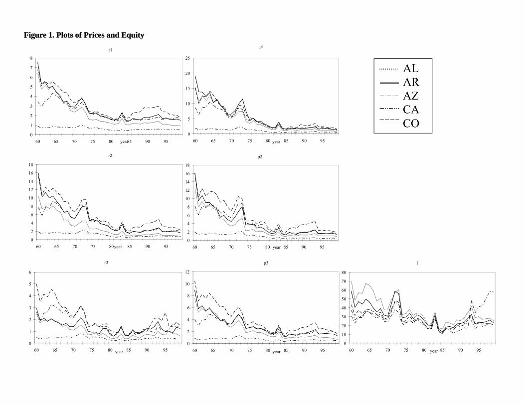
Figure 1. Plots of Prices and Equity

r1

0

1

2

3

4

5

6

7

8

60 65 70 75 80 85 90 95year

p1

0

5

10

15

20

25

60 65 70 75 80 85 90 95year

r2

0

2

4

6

8

10

12

14

16

18

60 65 70 75 80 85 90 95year

p2

0

2

4

6

8

10

12

14

16

18

60 65 70 75 80 85 90 95year

r3

0

1

2

3

4

5

6

60 65 70 75 80 85 90 95year

p3

0

2

4

6

8

10

12

60 65 70 75 80 85 90 95year

I

0

10

20

30

40

50

60

70

80

60 65 70 75 80 85 90 95year

ALARAZCACO