Individual Lab Report #7

Feb. 16, 2017

Menghan Zhang

TeamA

Amit Agarwal

Harry Golash

Yihao Qian

Zihao Zhang

Individual progress The work in these two weeks can be divided into 3 parts: 1. Got the verbal results of the detection algorithm.

The procedure is: load the SSD network and the pre-trained model, copy the output layer in vectors. Then wrap the input layer of the network in separate cv::Mat objects. After that process the image one by one. Finally save the output results. The format of detection results is [image_id, label, score, xmin, ymin, xmax, ymax]. Three things need to be address: First, the cpp file needs at least three inputs, including model file, weight file, and a file include the paths of the pictures to be detected. Also the threshold of detection score was modified, I changed it to 0.5, which means only the detection results which have confidence greater than 50% can be saved. Finally, there was one problem in the model pre-trained by author, the hyper parameter out_parameter did not match the actual output parameter, so I just deleted that. Command is shown below: build/examples/ssd/ssd_detect.bin models/VGGNet/VOC0712/SSD_300x300/deploy.prototxt models/VGGNet/VOC0712/SSD_300x300/VGG_VOC0712_SSD_300x300_iter_60000.caffemodel test.txt

2. Calculated and visualized the depth of the objects

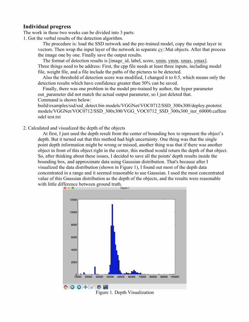
At first, I just used the depth result from the center of bounding box to represent the object’s depth. But it turned out that this method had high uncertainty. One thing was that the single point depth information might be wrong or missed, another thing was that if there was another object in front of this object right in the center, this method would return the depth of that object. So, after thinking about these issues, I decided to save all the points' depth results inside the bounding box, and approximate data using Gaussian distribution. That's because after I visualized the data distribution (shown in Figure 1), I found out most of the depth data concentrated in a range and it seemed reasonable to use Gaussian. I used the most concentrated value of this Gaussian distribution as the depth of the objects, and the results were reasonable with little difference between ground truth.

Figure 1. Depth Visualization

The result is show in table 1 and Figure 2. Table 1 Detection Results

Image Paths Label Depth(m) Location(xmin, ymin, xmax, ymax) examples/images/l-6.jpg 6(bus) 43.33 1441 691 1887 854 examples/images/l-6.jpg 7(car) 13.09 0 777 416 1130 examples/images/l-6.jpg 7(car) 23.6 860 764 1337 938 examples/images/l-6.jpg 7(car) 29.38 792 772 1015 888 examples/images/l-6.jpg 7(car) 45.56 1353 728 1521 838 examples/images/l-6.jpg 7(car) 39.06 680 775 883 874

Figure 2. Visualization 3. Tracking Research

I did some research on the RGB tracking this week, and most of the algorithm couldn’t achieve real-time tracking. The accuracy did not have much difference among the algorithms proposed recently, it's around 50 to 60 percent. Because of that, I choose the fastest two algorithms to learn more.

1. Learning by tracking: Siamese CNN for robust target association (around 50 FPS) 2. Learning to Track at 100 FPS with Deep Regression Networks(GOTURN) Siamese CNN is implement in Matlab and since we are going to use C++ and Linux to build the

platform, it will take us more time to transplant that into our system. I chose GOTURN and tested it.

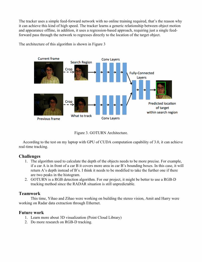
The tracker uses a simple feed-forward network with no online training required, that’s the reason why it can achieve this kind of high speed. The tracker learns a generic relationship between object motion and appearance offline, in addition, it uses a regression-based approach, requiring just a single feed-forward pass through the network to regresses directly to the location of the target object.

The architecture of this algorithm is shown in Figure 3

Figure 3. GOTURN Architecture.

According to the test on my laptop with GPU of CUDA computation capability of 3.0, it can achieve real-time tracking.

Challenges 1. The algorithm used to calculate the depth of the objects needs to be more precise. For example,

if a car A is in front of a car B it covers more area in car B’s bounding boxes. In this case, it will return A’s depth instead of B’s. I think it needs to be modified to take the further one if there are two peaks in the histogram.

2. GOTURN is a RGB detection algorithm. For our project, it might be better to use a RGB-D tracking method since the RADAR situation is still unpredictable.

Teamwork

This time, Yihao and Zihao were working on building the stereo vision, Amit and Harry were working on Radar data extraction through Ethernet. Future work

1. Learn more about 3D visualization (Point Cloud Library) 2. Do more research on RGB-D tracking.