Embed Size (px)
Citation preview
IDEC Discussion Paper No.10, Sep., 2013.
Indonesian Trade: Understanding the Duration and the Determinants of Its Hazard Rate
Anna Triana Falentina and Masaru Ichihashi

IDEC Discussion Paper No.10, Hiroshima University, Sep., 2013
1
Indonesian Trade: Understanding the Duration and the Determinants of Its Hazard Rate
Anna Triana Falentina1 and Masaru Ichihashi2
Abstract, Over the last two decades (1990-2011), Indonesian trade showed an increasing growth rate. The value of Indonesian exports and imports increased tenfold with other ASEAN countries and sixfold with non-ASEAN countries. During this period, Indonesian trade was dominated by trade with non-ASEAN countries (>79%), while intra-ASEAN accounted for almost 21%. In order to have trades occur in the first place, it is important to have not only a flourishing trade flows but also sustainable ones (Hess and Persson, 2011). Therefore, it is important to understand the process by which trades are sustained and trade flows grow in volume. Regarding the important role of trade duration, it’s crucial to investigate those of Indonesian trade with its partners. Therefore, this paper tries to explore the duration of Indonesian trade and to identify the factors that affect its hazard rate. This paper offers a new insight to accumulated studies of Indonesian trade which rarely discuss the impact of trade duration. This study uses discrete time-of-duration analysis which is suitable for trading data and repeated events, and is the first to apply the concept of duration to Indonesian trade. In our aim to explore the duration of Indonesian trade, we start by performing a thorough descriptive analysis. We found that most of Indonesian trade flows are short-lived; the median duration is merely 2 years for all spells, independent of whether one considers imports or exports. However, some trade flows last longer. These consist of essential imports such as wheat and export goods in which Indonesia has a strong comparative advantage (e.g. palm oil, rubber). Moreover, in many instances there is evidence of trade being frequently interrupted (‘stopped and re-started’). In our aim to identify the factors that affect the hazard rate, we performed a separate regression analysis for import and export. We estimate the baseline specification using discrete-time probit, logit, and cloglog models which include random effects for every partner-product-trade flow combination. We found factors that have impacts on hazard rate of stopping import (export) are distance, partner countries, initial trade value, market size, supplier size (only for import), the growth of credit ratio, exchange rate and product type. Moreover, we found that trading with developed countries as well as trading differentiated product has a lower hazard rate of stopping trade.
Keywords: Duration of trade, Discrete-time of Duration Analysis, ASEAN
JEL: F10; F13 1 Correspondening author. [email protected]. Graduate School for International Development and
Cooperation (IDEC), Hiroshima University, 1-5-1 Kagamiyama, Higashi-Hiroshima 739-8529, Japan. TELP:+81-
82-424-6905; FAX:+81-82-424-6904

IDEC Discussion Paper No.10, Hiroshima University, Sep., 2013
2
1. Introduction
Over the last two decades (1990-2011), Indonesian trade showed an increasing growth rate.
The value of Indonesian exports and imports increased tenfold in nominal US dollar terms with
other ASEAN countries and sixfold with non-ASEAN countries. These indicate that, in general,
Indonesian trade is growing. In addition, Indonesian trade was dominated by trade with non-
ASEAN countries (>79%), while intra-ASEAN accounted for almost 21% (Table 1 and Figure 6).
In order to have trades occur in the first place, it is important to have not only a growing
trade flows but also sustainable ones because factors causing existing trade flows to die could be
as much of an impediment to long-term trade growth (Hess and Persson, 2011). Therefore, from
a practical policy point of view it is important not only to understand the factors driving entry
into trading but also to understand the process by which trades are sustained and trade flows
grow in volume. For instance, in regards to export, successful export growth and diversification
require not only entry into exporting but survival (i.e. ability of a given country to continue
trading a particular product to a particular destination from year to year) and subsequent growth
(Brento, Pierola, and Uexkull, 2009).
Regarding the important role of trade duration, it’s crucial to investigate those of Indonesian
trade. Therefore, the general objective of this study is to identify the pattern of Indonesian trade
with its partners during 2000-2011. The specific purposes are to explore the duration of
Indonesian trade, and to identify the factors affecting the hazard rate. This paper tries to answer
the following questions: (1) How long is the duration of Indonesian trade? (2) What factors
affect the hazard rate of Indonesian trade? (3) Which bilateral trade has a lower hazard rate? (4)
Which commodity has a lower hazard rate?
This paper offers a new insight to accumulated studies of Indonesian trade which rarely
discussed on trade duration. Despite an emerging body of literature on trade at the country-
product level, the duration of trade has not received much attention until very recently. Moreover,
most of the previous studies on trade duration used Kaplan Meier and Cox Model which were
limited to one-spell observation or only for the first spell of multiple-spell observation, contrast
to the fact that trade data showed multiple-event characteristic (Brento, Pierola, and Uexkull,
2009). This study uses discrete-time of duration analysis which is suitable for trading data and be
the first to apply on Indonesian trade with ASEAN as well as non-ASEAN countries.

IDEC Discussion Paper No.10, Hiroshima University, Sep., 2013
3
This paper focuses on Indonesian bilateral trade relationships (import and export) with
partners of four (4) ASEAN countries, namely Philippines, Malaysia, Thailand, and Singapore,
and four major trading partners, i.e., Japan, 27 Europe Union Countries [EU (27)], China, and the
United States (US) from 2000 to 2011.
The remainder of the paper is organized as follows. Section 2 offers an overview of the
relevant empirical and theoretical literature. The data and empirical strategy are outlined in
Section 3, followed by a descriptive analysis of the Indonesian trade duration in Section 4.
Section 5 presents the regression analysis, and Section 6 summarizes and concludes.
2. Literature Studies
The studies concerning trade duration is quite limited. The first research on trade duration by
Besedes and Prusa (2006a, 2006b) has shown that the duration of trade relationships in the US
tend to be short with numerous entries and exists (leading to multiple spells) in a market. Using
data on US imports at the 7-digit (US Tariff Schedule) level from 160 exporters for 1972–1988
to estimate Kaplan–Meier survival functions, their results suggest that the duration of exports to
the United States is in general very short. The estimated survival rate is 67% for the first year,
thereafter decreasing at a decreasing rate.
As their companion paper, Besedes and Prusa (2006b) make use of the same US import data
as Besedes and Prusa (2006a). Basing their investigation on the model by Rauch and Watson
(2003), they add the Rauch (1999) classification of goods into homogeneous, reference-priced
and differentiated. Applying a Cox proportional hazards model, which—unlike the Kaplan–
Meier methodology—enables them to include explanatory variables in their analysis, they find
that differentiated products have lower hazard rates than homogeneous goods. They also find that,
within each product type, the larger the initial value of the trade flow, the longer the duration.
The prevalence of short-lived trade relationships has been also found in (Nitsch, 2009) for
German imports; Besedes and Blyde (2010) for the exports from Latin American countries;
Brento, Pierola, and Uexkull (2009) of developing countries export from 82 exporting countries
to 53 importers; Rudi, Jason and Peterson (2012) of the US Fresh Fruit & Vegetable Market, and
Obashi (2010) of Intra-East Asian machinery trade.
Nitsch (2009) examines the duration of German imports at the 8-digit (Combined
Nomenclature) product level, using data from Eurostat for 1995–2005. Employing a stratified

IDEC Discussion Paper No.10, Hiroshima University, Sep., 2013
4
Cox proportional hazards model, he investigates the effects of numerous regressors on the hazard
rate. The conclusions are that exporter characteristics (such as GDP and language), product
characteristics (such as unit values) and market characteristics (such as the import value, and
market share) affect the duration of German imports.
Besedes and Prusa (2011) focus on the extensive and intensive margins of trade. Using data
on manufacturing exports at the 4-digit Standard International Trade Classification (SITC)
Revision 1 level from 46 countries to 181 importers for 1975–2003, they decompose export
growth into three parts: establishing trade with new partners and markets (extensive margin);
having relationships survive or persist, and deepening existing relationships(intensive margin).
Estimating Kaplan–Meier survival functions for each of the Individual exporters, they find that
export duration is very brief, with the median being 1–2 years.
Nevertheless, a study by Brenton, Sabarowski and Uexkull (2009) found that unobserved
individual heteronegeity in product-level export flow data prevails, which questions previous
studies that have used Cox Proportional hazards model to model export survival, e.g. (among
others are) Besedes and Prusa (2006a); Obashi (2010); and Rudi, Jason and Peterson (2012).
Brenton, Sabarowski and Uexkull (2009) look at the duration of export flows at the 5-digit SITC
level from 82 exporters to 53 importers over the period 1985–2005, using a discrete time
complementary log-log model to estimate the effects of various explanatory variables on the
hazard rate. They found that trade in general was short-lived; also they found that the initial size
of an export flow, cultural & geographic ties between trading partners, market size and exporting
experience are important determinants of its survival.
In addition, a number of studies focused on factors affecting duration of trade. For instance,
Fugazza and Molina (2009) evaluated trade of 96 countries during 1995 to 2004 using extended
Cox model where the estimation coefficients are allowed to vary over duration time, found that
duration of trade increases with the region level of development. Other factors such as type of
product, export cost and the size of export also matter. Brento, Pierolla and Uexkull (2009) use a
Cox model to estimate determinants of trade in a data set with 44 exporters and 56 importers
over a 21-year period. Their research indicated that the size of initial export flow, search cost
exchange rate volatility are factors of hazard rates.

IDEC Discussion Paper No.10, Hiroshima University, Sep., 2013
5
Hess and Persson (2011) investigated the duration of EU imports from the rest of the world.
They employed a rich data set of detailed imports to individual EU-15 counties from 14 non-EU
exporters, covering the period 1962-2006. They performed descriptive analysis and regression
analysis using discrete-time duration models with proper control for unobserved heterogeneity.
They found that EU imports from the rest of the world are very short-lived, with median of 1-
year. In addition, they found that a set of statistically significant determinants of the duration of
trade. Among them is export diversification – the number of products exported and the number
of market served with the given product- which lowering the hazard of trade flows from dying.
Among the previous papers on the duration of country-level trade flows, there exist a
number of similarities. Not only do they all find the existence of short trade durations, but the
majority also study much shorter time periods while using estimation methods that introduce risk
of biases and misleading conclusions (see Hess and Persson 2012, for a discussion). However, at
this point there is no given theoretical model that can fully explain the observed short trade
durations. Neither sunk cost theory nor product life cycle theory could explain the short trade
duration (Hess and Person, 2011). Most of the literature about Indonesian trade focused on
factors that affect the Indonesian trade (value) relationship (e.g. Jongwanich, 2010); very limited
focus was on the duration of the relationship. In addition, studies on international trade duration
did not specifically explore the duration of Indonesian trade nor the factors affect it. Therefore,
there is still a very wide space for research on Indonesian duration trade, in which improving
survival rates is a key component of a country’s trade strategy (Fugazza and Molina, 2009).
3. Methodology of Analysis
3.1 Duration (Survival) Analysis
Survival analysis involves the modeling of time to event data; in this context, death or
failure is considered an “event”. In this paper, the failure or event is Indonesia stop trading, that
is stop importing (exporting) a specific product to (from) a specific partner, in other word exit
the market. Survival analysis in econometric model is known as the duration models.
Duration analysis unifies a range of models from continuous to discrete time, from non-
parametric to parametric and from those with or without accounting for unobserved
heterogeneity between the subjects. The data used in this paper is at product-level, thus the
survival rate refers to the product survival rate.

IDEC Discussion Paper No.10, Hiroshima University, Sep., 2013
6
Table 1. Illustration for Counting the Number of Spells and (Total) Duration (Product-Data)
Product - Trade Flow Trade Partners
2000
2001
2002
2003
2004
2005
2006
2007
2008
2009
2010
2011
No
year
s in
(dur
atio
n)
# Sp
ells
Petro
leum
gas
es –
Exp
ort Malaysia X X X X X X X X X X X X 12 1
Thailand X X X X X X X 7 1 Philippines X X X X X 5 1 Singapore X 1 1 Japan X 1 1 US X X X X X X X X X X X 11 2 China X X X X X X X 7 2 EU (27) X X X 3 2
Parts
of v
ehic
le –
Impo
rt
Malaysia X X 2 2 Thailand X X X X X X 6 3 Philippines X X X X X X X 7 3 Singapore X X X X X 5 3 Japan X X X 3 3 US X X X X 4 4 China X X X X X X 5 5 EU (27) X X X X X X 6 5
For each calendar year, we observe the value of Indonesia’s import (export) to (from) a
partner at the 6-digit product level. For every combination of partner, traded product, and trade
flow type (import/export), hereafter, referred to as a trade relationship, we calculate the duration
of trade as the number of consecutive years with non-zero imports (exports). A trade spell is
defined as a period of time with uninterrupted import (export) of a given product to (from) one
specific partner country. These different spells of trade constitute the core units of analysis in our
empirical study. The number of spells differs from the number of trade relationships since any of
the trading parties may choose to terminate the trade relationship and receive it a later point in
time. Henceforth, we will refer to such reoccurring trade relationships as multiple spells of
service.
We use product-data to perform a descriptive analysis of the duration of Indonesia imports
and exports, and we use product-period data to search for potential determinants of hazard rate in
a formal regression analysis. The product-period data was constructed in a 12-year panel of
product-period combination for each of the trade flow type (import/export). An event dummy
variable is created, that is 1 if trade stopped in that respective period, 0 otherwise. Moreover,

IDEC Discussion Paper No.10, Hiroshima University, Sep., 2013
7
there are some covariates, that is time-invariant (e.g. dummy partner, initial trade value, etc), and
time-variant variables (e.g. market/supplier size, exchange rate, growth of credit, etc).
3.2 Discrete-time model
A discrete time duration process is an approach to duration processes that consider events
occur at discrete points in time. International trade is traditionally observed once a year, even
though the underlying trade transactions may take place every day of the year, or, at the extreme,
only once a year. This implies that the observed durations of trade will be grouped into yearly
intervals. In general, this type of discrete duration data is known as discrete grouped duration
data since observations are grouped in terms of the interval of time in which an event occurs.
Discrete-time survival models are specified in terms of the discrete-time hazard, defined as
the conditional probability of the event occurring at a time point given that it has not already
occurred. A conventional feature of these survival models is that they become models for
dichotomous responses when the data have been expanded to so-called product-period data.
Standard logit and probit models can then be used, as well as complementary log-log models
(Beck, Katz, and Tucker, 1998).
We followed Hess and Persson (2012) who recommend the use of discrete-time models for
trade duration analysis. In brief, the continuous time model, such as the Cox model, has three
major drawbacks when applied to large trade data sets. First, it faces problems in the presence of
many tied duration times, leading to biased coefficient estimates and standard error. Second, it is
difficult to properly control for unobserved heterogeneity, which can lead to parameter bias and
bias in the estimated survivor function. Third, the Cox model imposes the restrictive and
empirically questionable assumption of proportional hazards. In contrast, with discrete-time
models there is no problem handling ties; unobserved heterogeneity can be controlled without
difficulty, and the restrictive proportional hazards assumption can easily be bypassed.
3.3 Empirical Models
Let Ti be a continuous, non-negative random variable measuring the survival time of a
particular trade relation. In a discrete-time framework, the core of duration analysis is formed by
the probability that a particular trade relation terminates in a given time interval [tk , tk+1), k = 1,
2, . . ., kmax, and t1 = 0, conditional on its survival up to the beginning of the interval and given

IDEC Discussion Paper No.10, Hiroshima University, Sep., 2013
8
the explanatory variables included in the regression model. This conditional probability is termed
the discrete-time hazard rate and formally defined as
),(),|(: '1 kikikkikiik xFxtTtTPh γβ +=≥<= + (1)
where xik is a vector of possibly time-varying covariates, γk is a function of (interval) time that
allows the hazard rate to vary across periods (somewhat loosely, we will refer to γk as the
grouped-duration baseline hazard, although this is not formally correct in all instances), and F(.)
is an appropriate distribution function ensuring that 0 ≤ hik ≤ 1 for all i, k. In our case, the
subscript i denotes separate spells of trade relationships (i = 1, . . . , n) for any given partner-
product-trade flow type combination.
For each trade spell, the last year in which a positive trade volume was observed, can be
recorded. In the following, this terminal time period is denoted ki , the subscript i indicating that
it may differ across spells. Introducing a binary variable, yik , taking the value one if spell i is
observed to cease during the kth time interval, and zero otherwise, the log-likelihood for the
observed data is given by: ∑∑= =
−−+=n
i
k
kikikikik
i
hyhyL1 1
)]1ln()1()ln([ln (2)
This expression is structurally isomorphic to a standard log-likelihood function for a binary
panel regression model with dependent variable yik3. This allows discrete time hazard models to
be estimated by binary dependent variable methods and time-varying covariates to be
incorporated.
To be able to estimate the model parameters, a functional form for the hazard rate hik needs
to be specified. The most commonly encountered functional specifications are the normal,
logistic, and extreme-value minimum distribution, leading to a probit, logit, or cloglog model,
respectively. In addition, unobserved heterogeneity can be accounted for by including random
effects into the binary choice model framework above. Applying conventional binary response
panel data models with normal random effects is a sensible approach when estimating discrete-
time duration models (Hess and Person, 2012).
3 To obtain consistent parameter estimates from this log-likelihood, each spell must be independent of all other spells, censoring must occur only at interval boundaries, and censoring must not provide any information about Ti beyond that available in the covariates (see e.g., Singer and Willett 1993 for excellent surveys on the derivation of the likelihood).

IDEC Discussion Paper No.10, Hiroshima University, Sep., 2013
9
3.4 Link Functions
In our aim to identify factor affecting hazard rate, we start by making the hazard rate of
stopping import (export), conditional on covariates as well as survival as in equation (1). We
need an admissible distribution function. Three are common, logit, probit and cloglog.
The notion of unobserved heterogeneity amounts to observations being conditionally
different (heterogeneous) in terms of their hazards in ways that are unaccounted for in the
systematic part of our models, which can be particularly bad in duration models (i.e., spurious
duration and/or inconsistent estimation). Therefore, in order to relax the assumption of
conditional independence among the responses for the same items (partner-product combination)
given the covariates, we can include a product-specific random intercept ζi in the linear predictor
to obtain a random-intercept logistic regression model:
A. Logit ikikik
ik xh
hζγβ ++=
−
'
1log (3)
The random intercepts ),0(~ ψζ Ni are assumed to be independent and identically
distributed across items i and independent of the covariates 'ikx . The random intercept can be
thought of as the combined effect of omitted item-specific (time-constant) covariates that cause
some items to be more prone to stop being traded than others. It is appealing to model this
unobserved heterogeneity in the same way as observed heterogeneity by simply adding the
random intercept to the linear predictor. Odds ratios obtained by exponentiating regression
coefficients in this model must be interpreted conditionally on the random intercept and are
therefore often referred to as conditional or subject-specific odds ratios.
B. Probit ( )ikikik xh ζγβφ ++= ' (4)
C. Cloglog }}exp{exp{1 'ikikik xh ζγβ ++−−= (5)
3.5 Data /Materials
This paper uses annual bilateral export and import data at the six-digit level of Harmonized
System (HS) 1996 from 2000 to 2011 obtained from the UN Comtrade. The HS six-digit level is
the most detailed disaggregated level of trade data that is internationally comparable and
publically available. Moreover, this paper also utilizes data of DOT IMF, bilateral gravity data
from EPII, WDI-WB, ASEAN Statistics, IFS-IMF, and UN Statistics.

IDEC Discussion Paper No.10, Hiroshima University, Sep., 2013
10
The variables that are used in this study are common variables in a gravity model. The
gravity variables have been very successful in explaining trade volumes; therefore, they might
have a role in explaining the duration of trade as well (Besedes and Blyde, 2010). All the
continuous variables are in logarithm form, except growth of credit ratio. Due to
multicollinearity problem, variable log of credit ratio is replaced by growth of credit ratio.
4. Trade Pattern Analysis
4.1 Trade Duration
In our aim to explore the duration of Indonesian trade, we start by performing a thorough
descriptive analysis. Table 5 offers some initial summary statistics as to the length of Indonesian
trade flows. As it can be seen, the median duration of all spells is 2 years, both for import and
export. The most common scenario is, in other words, for Indonesia to go from not importing
(exporting) the product from (to) partner’s market for at most 2 years, only to then leave the
market again. The mean duration of more than 4 years for import and more than 3 years for
exports are also rather low.
Table 2. Summary Statistics
IMPORT
Type of spell
Length of Observed spell Total number of spells
Fraction of spells left-censored
Total number of trade
relationships
Total number of product
codes Median Mean
All spells 2 4.756 59,594 0.29 35,355 5,098 Single spell 12 9.149 19,634 0.65 19,634 4,926 First spells 4 6.187 35,355 0.36 35,355 5,098
EXPORT
Type of spell
Length of Observed spell Total number of
spells
Fraction of spells left-censored
Total number of trade
relationships
Total number of product
codes Median Mean
All spells 2 3.706 57,252 0.12 32,521 5,027 Single spell 9 7.055 16,207 0.43 16,207 4,832 First spells 2 4.704 32,521 0.22 32,521 5,027
Table 2 also shows the median and means for other type of spell that is single-spell and first-
spell. Single spells, i.e. observations where a specific partner-product-trade flow type
combination has only one single coherent period of trade. In addition, we disregard all higher-
order spells to see whether the first observed spell has different characteristics. Even though the
number of observations is drastically reduced (implying that we have a substantial amount of

IDEC Discussion Paper No.10, Hiroshima University, Sep., 2013
11
trade flows that die and then reoccur), the median duration of trade is 4 years (import) and is
only 2 years (export) for first spell, while the median is 12 year (import) and 9 years (export) for
single-spell.
The first-spell type indicates similar patterns but a bit longer duration before the trade
terminated (for the first time). The median of trade durations are 4 years for import and 2 year
for export, while the mean are more than 6 years and more than 4 years for import and export
respectively. On the other hand, the single-spell type shows that the median duration for import
and export are 12 years and 9 years, respectively, with mean 9 years (import) and 7 years
(exports). These indicate that for certain products, trade is long lasting.
Comparing the all spell figure to with what has been found for other countries; Indonesian
trade appears to be at least as short-lived. For instance, Hess and Person (2011) find a
corresponding median duration of 1 year for EU imports, while Besedes and Prusa (2006a) find
2-year median duration for US imports at the same level of data aggregation (with mean of over
4 years). Nitsch (2009), who uses much more detailed data, finds a median duration of 2 years
for German imports, suggesting that German imports are more long-lived than imports to other
EU-15 countries. Moreover, Besedes and Blyde (2010) found evidence confirming that export
relationships in Latin America are in general short-lived but that significant differences across
regions exist with Latin America exhibiting lower export survival rates than the US, the EU and
East Asia, among others. Thus, the data suggest that Indonesian trades are at least as short-lived
as those for other countries and possible even more so.
Focusing now on the length of a spell before it terminated (see Table 6 in appendix), we
found that for import, more than one-third of all spells cease during the first year of service.
Approximately 50% of all trade flows terminate within the first 2 years, and less than 8% of
trade flows last only a maximum of 3 years; meaning that after serving for several years, trade
flow stopped. In addition, less than 1% of all relationships survive for the first 11 years.
However, a moderate percentage that is, more than 21% of trade, occurred for 12 years, without
any break exiting the market, which points out that for certain products, once trade was
established, it survived. In the same way, single-spell and first-spell types also showed a similar
duration. Thus, the vast majority of spells will last only for at most a few years and only a small
fraction can be characterized as long-lasting.

IDEC Discussion Paper No.10, Hiroshima University, Sep., 2013
12
Similarly, export trade also indicated a typical pattern with those of import. More than 60%
of all observed spells exist only within the first two years of service. On the other hand, more
than 12% last for 12 years, as once trade started it survived without exiting the market. These are
also parallel to those of single-spell and first-spell. Our conclusion so far is that Indonesian
trades are short-lived.
4.2 Trade Stability
Table 3 depicts the stability of import and export that is the number of consecutive years of
positive trading (spells). The more the number of spells, the more the number of breaks (stop
trading) and trade reoccurrence. As it can be seen more than 55% of trade last in one spell, i.e.
after serving for several years then it stopped. While more than a quarter of trade was occurred in
two spells. On the other hand, less than 20% of trade established with more than 3 spells which
were disrupted for more than two times of exiting the market. These indicate that Indonesian
import and export trade were quite stable, a small portion that is multi-event characteristic, i.e.
multiple entries and exits the market. For some years trade occurred then in the next year is
stopped, and by the next year it started again.
Therefore, from the above explanation regarding Indonesian trade duration and stability we
can conclude that Indonesian trades are generally short-lived, while some products enjoy a long-
lasting trade relationship; yet it is quite stable with a small portion of multiple exits and entries of
the market.
Table 3. Number of Trade Relationship by Spell Numbers
Import Export Spell No Freq. Percent Cum. Total
#spells Spell No Freq. Percent Cum. Total
#spells 1 19,634 55.53 55.53 19,634 1 16,207 49.84 49.84 16,207 2 9,074 25.67 81.2 18,148 2 9,718 29.88 79.72 19,436 3 4,952 14.01 95.21 14,856 3 4,960 15.25 94.97 14,880 4 1,522 4.3 99.51 6,088 4 1,456 4.48 99.45 5,824 5 170 0.48 99.99 850 5 175 0.54 99.98 875 6 3 0.01 100 18 6 5 0.02 100 30
Total 35,355 100 59,594 Total 32,521 100 57,252
5. Regression Analysis
In our aim to identify the factors affecting the hazard rate, we performed a separate
regression analysis for import and export. We estimate the baseline specification using discrete-

IDEC Discussion Paper No.10, Hiroshima University, Sep., 2013
13
time probit, logit, and cloglog models. All left-censored observations, which, if included, could
lead to bias in the estimated hazard rate (Hess and Persson, 2012), are excluded. In all models,
we include random effects for every partner-product-trade flow combination.
5.1 Results
The results of the estimations can be found in Table 12. As we can see that for both import
and export estimations:
1. Based on the probability of Likelihood Ratio (LR), the coefficient is statistically different
from zero. Therefore, we conclude that the model fit the data well. The logit model gave the
highest log likelihood value.
2. Likelihood-ratio tests strongly reject the null hypothesis of no latent heterogeneity for all
model specifications ( ρ =0), implying that unobserved heterogeneity plays a significant role
in all model specifications and should not be ignored.
3. All of the variables are statistically significant, except supplier size for export, with sign of
the coefficients are as expected.
In the trade literature, two countries with a short distance between them are often expected
to have lower costs for trading. It seems reasonable to assume that, everything else being equal,
higher trade costs should make a trading relationship more vulnerable to negative shocks and
increase the likelihood of failure. Therefore we would expect distance to increase the hazard. To
control for this factor we include the logarithm of the distance between the trading countries’
capitals. The estimated parameters for import and export support these hypotheses: distance has a
significantly positive coefficient.
We included dummy variable for trading with developed countries, that is Japan, US, and
EU(27) to see if there is any difference between trading with developed countries and with
developing countries. Fugazza and Molina (2009) found that trading with developed countries
has a lower hazard rate than those involving developing countries. Thus, the hypothesis would be
trading with developed countries would have a lower hazard rate. This hypothesis is supported
by the result, that is having developed countries as partners of import (export) have longer-
lasting relationships than import (export) flows from developing countries.

IDEC Discussion Paper No.10, Hiroshima University, Sep., 2013
14
Table 4. Factors Affecting Trade Duration
Variables/Indicators Model
Logit Probit Cloglog
Log-odds Odds Ratio IMPORT
Log Distance 0.514854*** 1.673395*** 0.300776*** 0.323749*** Developed Country Dummy -0.39716*** 0.672226*** -0.23074*** -0.24515*** Log Initial Trade Value -0.10342*** 0.901751*** -0.06054*** -0.06819*** Log Market Size (GDP Indo) -0.18921*** 0.827612*** -0.11257*** -0.10169*** Log Supplier Size (GDP partners) -0.32166*** 0.724947*** -0.18851*** -0.20595*** Growth Credit Ratio -0.00564*** 0.994378*** -0.00332*** -0.00363*** Log Real Exchange Rate 0.137567*** 1.147479*** 0.080696*** 0.088371*** Differentiated Product Dummy -0.3644*** 0.694615*** -0.21371*** -0.23728*** Constant 10.84521*** N/A 6.407773*** 6.017986*** Observations 130,020 130,020 130,020 130,020 No. of spells 46,807 46,807 46,807 46,807 Trade relations 22,568 22,568 22,568 22,568 Log likelihood -164,851.21 -164,851.21 -165,120.23 -165,670.86 Prob LR coeff=0 0.000 0.000 0.000 0.000 ρ 0.302218 0.302218 0.330073 0.271447 Prob LR rho=0 0.000 0.000 0.000 0.000 EXPORT
Log Distance 0.522115*** 1.685588*** 0.305507*** 0.324416*** Developed Country Dummy -0.79212*** 0.452883*** -0.46422*** -0.49427*** Log Initial Trade Value -0.12326*** 0.884036*** -0.07207*** -0.07587*** Log Market Size (GDP partners) -0.08633*** 0.917293*** -0.05014*** -0.0524*** Log Supplier Size (GDP Indo) -0.01835 0.98182 -0.00962 0.018243 Growth Credit Ratio -0.00619*** 0.993828*** -0.00375*** -0.00420** Log Real Exchange Rate -0.16944** 0.844134** -0.09668** -0.04415 Differentiated Product Dummy -0.45037*** 0.63739*** -0.26333*** -0.27595*** Constant 2.258984*** N/A 1.259395** -0.44209 Observations 127,896 127,896 127,896 127,896 No. of spells 50,229 50,229 50,229 50,229 Trade relations 25,498 25,498 25,498 25,498 Log likelihood -184,480.94 -184,480.94 184,805.16 -185,748.89 Prob LR coeff=0 0.000 0.000 0.000 0.000 ρ 0.29179 0.29179 0.318311 0.240415 Prob LR rho=0 0.000 0.000 0.000 0.000 Significant at ***) α = 1%; **) α = 5%; ρ denotes the fraction of the error variance that is due to variation in the unobserved individual factors. The number of observations is given by the total number of years with positive trade for all trade relationships.

IDEC Discussion Paper No.10, Hiroshima University, Sep., 2013
15
Furthermore, the supplier size variable (partner’s GDP) is included in Indonesian import as a
proxy to control for supply capacity, while the market size variable (Indonesia’s GDP) is
included as a proxy for demand size. In contrast, in export we include the supplier size variable
(Indonesia’s GDP) as a proxy to control for supply capacity, while the market size variable
(partner’s GDP) is included as a proxy for demand size. We expect that higher supply capacity
and higher demand size will lower the hazard. This supplier size hypothesis is supported by the
results of import only while in export it is not significant. The supplier size has a significantly
negative coefficient for import which would suggest that import trading relationships involving
economically large supplier are less likely to die. At the same time, the market size is significant
with the expected sign for import and export, which indicates that for Indonesian import (export),
market size is an important factor to have a lower hazard rate of trade. The bigger the market size
the longer the trade duration.
Our results are intuitive and consistent with many theoretical models. One might expect
relationships involving homogeneous goods to be quite fragile. There are a number of
explanations why differentiated products may exhibit long duration. Sunk costs and relationship
specific investments can also explain differences in duration. If differentiated goods require
larger initial investments, models such as that of Melitz (2003) suggest once relationships are
established they will tend to be robust. In a series of papers Rauch uses network and search
theory to explain why trade in differentiated products and homogeneous products is different
(among others Rauch and Trindade, 2002). Fugazza and Molina (2009) suggest that the
relationship between trade duration and the type of product portrays the degree of
competition/information patterns characterizing traded products.
In addition, we include growth of credit ratio as a proxy of financial system development.
Due to multicollinearity problem we replaced the log of credit ratio by growth of credit ratio.
The hypothesis would be partners in countries with more developed financial systems tend to
maintain their trade relationships longer. The results support this hypothesis: the coefficients are
negative and significant for both import and export, which implies that trading (import/export)
with more-developed-financial-system countries would have longer trade relationships.
We also include the log of the relative real exchange rate as a proxy of relative price changes,
since exchange rate movements could explain exits from (and entry into) the market. A

IDEC Discussion Paper No.10, Hiroshima University, Sep., 2013
16
depreciating exchange rate would decrease the import yet it increases the export, such that it
leads to a higher hazard rate for import and a lower hazard rate for export. This variable has a
significant and positive coefficient for import, suggesting that a depreciation of the Indonesia
currency (Rupiah) relative to the currencies of partners, as expected, increases the likelihood of
import failure. On the other hand, for export this variable has a significant and negative
coefficient, suggesting that a depreciation of the Rupiah relative to the currencies of partners, as
expected, decreases the likelihood of stopping export.
5.2 Interpretation
Since the logit model offers the best fit for our data, both for import and export, i.e. the
biggest log likelihood value, we will focus on this model when discussing the interpretation of
the estimation results. The logit model, however, represents the relationship of covariates to the
log odds of event. Therefore, in order to understand the impact of covariates to the probability of
stopping trade, we use marginal changes for continuous variable and discrete changes for dummy
variables.
Table 5. Marginal, Discrete and Factor Changes
Variable Marginal 01 Factor Change in Odds ratio
IMPO
RT
Log Distance 0.123 --- 1.673 Partner Dummy N/A -0.098 0.672 Log Initial Trade Value -0.025 --- 0.902 Log Market Size (GDP Indo) -0.045 --- 0.828 Log Supplier Size (GDP partners) -0.077 --- 0.725 Growth Credit Ratio -0.001 --- 0.994 Log Real Exchange Rate 0.033 --- 1.147 Product Type Dummy N/A -0.089 0.695
EX
POR
T
Log Distance 0.104 --- 1.686 Partner Dummy N/A -0.181 0.453 Log Initial Trade Value -0.025 --- 0.884 Log Market Size (GDP partners) -0.017 --- 0.917 Log Supplier Size (GDP Indo) Not sig (-0.004) --- 0.982 Growth Credit Ratio -0.001 --- 0.994 Log Real Exchange Rate -0.034 --- 0.844 Product Type Dummy N/A -0.098 0.637
Baseline: mean values, except partner dummy countries=0, product type dummy=0

IDEC Discussion Paper No.10, Hiroshima University, Sep., 2013
17
The marginal change can be interpreted as for one unit increase in a variable from the
baseline, the probability of an event, i.e. stopping import (export), is expected to
increase/decrease by the magnitude of marginal change, holding all other variables constant.
However, the marginal change is not applicable for dummy variable, instead we use discrete
change. The interpretation of discrete change is for a change from one group to another group of
a variable, the probability of an event is expected to change by the magnitude of discrete change,
holding all other variables at the given values. While using odds ratio, for a one unit increase in
an independent variable then the odds of stopping import (export) increases (if greater than one)
or decreases (if less than one) by a factor of the magnitude of a change in the odds ratio, holding
all other variables constant.
Finally based on the result, we can summarize a set of factors affecting the hazard rate of
stopping import (and export). Those are distance, partner countries, initial trade value, market
size, supplier size (only for import), growth of credit ratio, exchange rate and product type.
For Indonesian import, the farther the distance between Indonesia and trade partner, the
higher the hazard rate of stopping import. Importing from developed countries (as trade partners)
tends to have a long-lasting import relationship. The bigger the initial import values, the longer
import duration. The Indonesian market size matters to have lower hazard rate of stopping
import, that is the bigger the demand for import (the bigger the Indonesian market size) the lower
the hazard rate. Importing from larger supplier has a higher survival rate. Moreover, Importing
from partners that have a growing credit ratio tends to have longer import relationship. When
Rupiah depreciates it is less likely to keep importing (shorter import duration). Lastly, importing
differentiated product indicates longer import duration.
For export, the farther the distance between Indonesia and trade partner, the higher the
hazard of stopping export. Exporting to developed countries (as trade partners) tends to have a
long-lasting export relationship. The bigger the initial export values, the longer the export
duration. Exporting to bigger market is very likely to have longer export duration. However, the
Indonesian GDP (Indonesian supplier size) does not matter to have lower hazard rate of stopping
export. Exporting to partners that have a growing credit ratio tend to have longer export
relationship. In addition, when Rupiah depreciates it is more likely to keep exporting (longer
export duration). Finally, exporting differentiated product indicates longer export duration.
IDEC Discussion Paper No.10, Hiroshima University, Sep., 2013
18
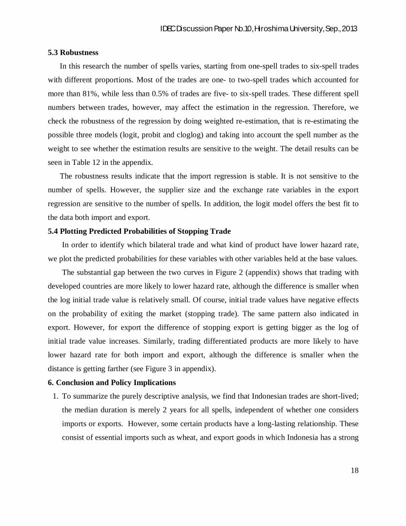
5.3 Robustness
In this research the number of spells varies, starting from one-spell trades to six-spell trades
with different proportions. Most of the trades are one- to two-spell trades which accounted for
more than 81%, while less than 0.5% of trades are five- to six-spell trades. These different spell
numbers between trades, however, may affect the estimation in the regression. Therefore, we
check the robustness of the regression by doing weighted re-estimation, that is re-estimating the
possible three models (logit, probit and cloglog) and taking into account the spell number as the
weight to see whether the estimation results are sensitive to the weight. The detail results can be
seen in Table 12 in the appendix.
The robustness results indicate that the import regression is stable. It is not sensitive to the
number of spells. However, the supplier size and the exchange rate variables in the export
regression are sensitive to the number of spells. In addition, the logit model offers the best fit to
the data both import and export.
5.4 Plotting Predicted Probabilities of Stopping Trade
In order to identify which bilateral trade and what kind of product have lower hazard rate,
we plot the predicted probabilities for these variables with other variables held at the base values.
The substantial gap between the two curves in Figure 2 (appendix) shows that trading with
developed countries are more likely to lower hazard rate, although the difference is smaller when
the log initial trade value is relatively small. Of course, initial trade values have negative effects
on the probability of exiting the market (stopping trade). The same pattern also indicated in
export. However, for export the difference of stopping export is getting bigger as the log of
initial trade value increases. Similarly, trading differentiated products are more likely to have
lower hazard rate for both import and export, although the difference is smaller when the
distance is getting farther (see Figure 3 in appendix).
6. Conclusion and Policy Implications
1. To summarize the purely descriptive analysis, we find that Indonesian trades are short-lived;
the median duration is merely 2 years for all spells, independent of whether one considers
imports or exports. However, some certain products have a long-lasting relationship. These
consist of essential imports such as wheat, and export goods in which Indonesia has a strong

IDEC Discussion Paper No.10, Hiroshima University, Sep., 2013
19
comparative advantage (e.g. palm oil, rubber). Moreover, in many instances there is
evidence of trade being frequently interrupted (‘stopped and re-started’).
2. Factors that have impacts on hazard rate of stopping import (and export) trade are distance,
partner countries, initial trade value, market size, supplier size (for import only), growth of
credit ratio, exchange rate and product type being traded.
3. The farther the distance, the higher the hazard of stopping import (export). Trading with
developed countries (as trade partners) tends to have a long-lasting import (export)
relationship. The bigger the initial trade values, the longer the trade duration. Trading
(import/export) to bigger market is very likely to have longer trade (import/export) duration
as demand gets bigger. Importing from larger supplier has a higher survival rate. Trading
with partners that have a growing credit ratio tend to have longer trade relationship. In
addition, when Rupiah is depreciating it is less likely to keep importing (shorter import
duration), yet it is more likely to keep exporting (longer export duration). Finally, trading
differentiated product indicates longer trade (import/export) duration.
4. For import, market size (Indonesia’s GDP) as well as supplier size (partner’s GDP) are
important to have lower hazard rate of stopping import. These indicate that Indonesian
import depends on both domestic and foreign situation. On the other hand, for export,
market size (partner’s GDP) matters for longer export duration, yet supplier size
(Indonesia’s GDP) does not matters which indicate that export depends more on foreign
situation.
5. Trading with developed countries has a lower hazard rate compare to developing countries.
6. Trading differentiated product has a lower hazard rate compared to non differentiated
product.
Some policy implications that can be drawn from this research are:
1. Many Indonesian exports, in terms of product-partner combination, are short lived. It is
important to investigate further how Indonesian exports have been growing. The growth in
export trade may be occurring more through increases volume of trade for existing trade
partners (the intensive margin) rather than increases in trade in new products or to new
partners (the extensive margin) (Besedes and Prusa, 2006a, 2006b). Also for the short

IDEC Discussion Paper No.10, Hiroshima University, Sep., 2013
20
duration of import. Further study investigating the cause of short trade duration is needed. If
it is found that constraint on financing is one of the issues then the government should
support for better financial system. Among other benefits that could be gained, it will also
help improve trade duration.
2. Any improvement in transportation which reduces transportation cost is very likely to
strengthen trade links.
3. Indonesia and other developing countries do not trade as much as those with developed
countries as they may produce similar products. However, the new trend of production
network in Asian countries showed that Indonesia, and other ASEAN countries and China
are part of the world production network. For instance, Indonesia produced “part &
components” of differentiated goods. At the same time Indonesia traded “final goods” of the
differentiated product to developed countries (Coxhead and Jayasuriya, 2010). Therefore, it
implies for specialization as the consumer may not consider the source of the product.
4. Brenton, Pierola and Uexkull (2009) suggested that the associated high hazard rate for
initially small flows suggests caution in public policy interventions that are aimed
specifically at exporters that start small.
5. Selling products to bigger countries and buying from larger markets are likely to have longer
trade relationships. Therefore, it is crucial to maintain trade relationships with them by
committing to the trade contract, such as fulfill the product specification requirements.
6. It needs to be further investigating what kind of exchange rate policy that best suit to
Indonesia according to its needs and trade objectives, always with the proviso that the
chosen regime must be credibly supported by policies consistent with the choice. As noted
by Michael Mussa, et.al (2000), that there is no single exchange rate regime that is best for
all countries in all circumstances. Which exchange rate regime and associated policies are
appropriate for a country depend on its particular circumstances.
7. As it is shown in discussion, type of product matters for survival, to be specific
differentiated product has a lower hazard rate. Further study is needed to identify whether
producing differentiated product produce good externalities. When such condition is proven,
then government should support this economic sector activity.

IDEC Discussion Paper No.10, Hiroshima University, Sep., 2013
21
References
1. Beck, N., Katz, J. N., & Tucker, R. (1998: 42 (4)). Taking Time Seriously: Time-Series-Cross-Section Analysis with a Binary Dependent Variable. American Journal of Political Science, 1260-1288.
2. Besedes, T., & Blyde, J. (2010). What Drives Export Survival? An Analysis of Export Duration in Latin America. http://siteresources.worldbank.org/.
3. Besedes, T., & Prusa, T. J. (2006). Ins, Outs, and The Duration of Trade. Canadian Journal of Economics Vol. 39, No. 1, 267-295.
4. Besedes, T., & Prusa, T. J. (2006b: 70 (2)). Product Differentiation and Duration of US Import Trade. Journal of International Economics, 339-358.
5. Besedes, T., & Prusa, T. J. (2011: 96). The Role of Extensive and Intensive Margins and Export Growth. Journal of Development Economics, 371-379.
6. Brenton, P., Pierola, M. D., & Uexkull, E. v. (2009). The Life and Death of Trade Flows: Undestanding the Survival Rates of Developing-Country Exporters. In T. W. Bank, Breaking into New Markets: Emerging Lesson for Export Diversification (pp. 128-295). Washington DC: The World Bank.
7. Brenton, P., Sabarowski, C., & Uexkull, E. v. (2009, March). What Explains the Low Survival Rate of Developing Country Export Flows. Policy Research Working Paper No. 4951 of The World Bank.
8. Coxhead, I., & Jayasuriya, S. (2010). China, India and the Commodity Boom: Economic and Environmental Implications for Low-income Countries. The World Economy, 525-551.
9. Fugazza, M., & Molina, A. C. (2009). The Determinants of Trade Survival. HEID Working Paper No. 05/2009.
10. Hess, W., & Persson, M. (2011 (147)). Exploring the Duration of EU Imports. Review of World Economics, 665-692.
11. Hess, W., & Persson, M. (2012 (43)). The Duration of Trade Revisited: Continuous-time versus discrettime hazards. Empirical Economics, 1083-1107.
12. Jongwanich, J. (2010). Determinants of Export Performance in East and Southeast Asia. The World Economy, 20-41.
13. Long, S. J. (1997). Regression Models for Categorical and Limited Dependent Variables. Advanced Quantitative Techniques in the Social Sciences. Sage Publications.
14. Melitz, M. J. (2003 (71)). The Impact of Trade on Intra-Industry Reallocations and Aggregate Industry Productivity. Econometrica , 1695-1725.

IDEC Discussion Paper No.10, Hiroshima University, Sep., 2013
22
15. Mussa, M., Masson, P., Swoboda, A., Jadresic, E., Mauro, P., & Berg, A. (2000). Exchange Rate Regimes in an Increasingly Integrated World Economy. Occasional Paper 193 IMF.
16. Nitsch, V. (2009: 145 (1)). Die Another Day: Duration in German Import Trade. Review of Wrold Economics, 133-154.
17. Obashi, A. (2010). Stability of Production Networks in East Asia: Duration and Survival of Trade. Japan and the World Economy 22 (2010) 21-30.
18. Park, H. M. (2004). Presenting Binary Logit/Probit Models Using the SAS/IML. http://www.iuj.ac.jp/faculty/kucc625/documents/Binary_Logit.pdf.
19. Rabe-Hesketh, S., & Skrondal, A. (2012). Multilevel and Longitudinal Modeling Using Stata Volume II: Categorical Responsesn, Counts, and Survival 3rd edition. Texas: Stata Press.
20. Rauch, J. E. (1999: 48). Networks versus Market in International Trade. Journal of International Economics, 7-35.
21. Rauch, J. E. (2007). Development through Synergistic Reform. NBER Working Paper Series 13170.
22. Rauch, J. E., & Trindade, V. (2002: 84 (1)). Ethnic Chinese Networks in International Trade. the Review of Economics and Statistics, 116-130.
23. Rauch, J. E., & Watson, J. (2003: 21 (7)). Starting Small im an Unfamiliar Environment. International Journal of Industrial Organization, 1021-1042.
24. Rudi, J., Grant, J., & Peterson, E. B. (2012). Survival of the Fittest: Explaining Export Duration and Export Failure in the U.S. Fresh Druit and Vegetable Market. AAEA Annual Meeting.
25. Singer, J. D., & Willet, J. B. (2003). Applied Longitudinal Data Analysis: Modeling Change and Event Occurrence. New York: Oxford University Press.
26. Stirbat, L., Record, R., & Nghardsaysone, K. (2013). Determinants of Export Survival in the Lao PDR. The World Bank Policy Research Working Paper 6301.
27. Sueyoshi, G. (1995: 10 (4)). A Class of Binary Response Models for Gruoped Data Duration. Journal of Applied Econometrics, 411-431.

IDEC Discussion Paper No.10, Hiroshima University, Sep., 2013
23
Appendices
Figure 1. Indonesian Trade, 1990-2011
Source: Directory of Trade, IMF
Table 6. Share of Indonesian Trade by Partners, 1990-2011
Partners Value of (Millions US$) Within Group To the World
Export Import Total Share Cumulative Share Share Cumulative
Share Intra-ASEAN 300,251.89 295,080.78 595,332.67
20.85%
Singapore 150,831.15 156,209.48 307,040.63 51.57% 51.57% 10.75% 10.75% Malaysia 65,955.88 59,245.45 125,201.33 21.03% 72.61% 4.38% 15.14% Thailand 37,853.56 53,223.42 91,076.98 15.30% 87.90% 3.19% 18.33% Philippines 25,247.03 10,522.94 35,769.97 6.01% 93.91% 1.25% 19.58% Vietnam 15,106.56 9,957.96 25,064.52 4.21% 98.12% 0.88% Myanmar 2,470.74 5,287.29 7,758.03 1.30% 99.43% 0.27% Cambodia 1,983.05 584.61 2,567.66 0.43% 99.86% 0.09% Brunei D. 757.98 37.79 795.76 0.13% 99.99% 0.03% Lao PDR 45.95 11.85 57.80 0.01% 100.00% 0.00%
Non-ASEAN 1,335,699.21 924,630.72 2,260,329.93
79.15% Euro Area 166,139.67 113,613.68 279,753.35 12.38% 12.38% 9.80% 29.37% Japan 349,988.83 170,092.76 520,081.59 23.01% 35.39% 18.21% 47.59% United States 184,130.45 101,382.24 285,512.69 12.63% 48.02% 10.00% 57.59% China, P.R. 118,591.79 121,579.92 240,171.71 10.63% 58.64% 8.41% 66.00% Other countries 516,848.47 417,962.12 934,810.59 41.36% 100.00% 32.74%
The World 1,635,951.10 1,219,711.50 2,855,662.60 100.00% Source: Directory of Trade, IMF

IDEC Discussion Paper No.10, Hiroshima University, Sep., 2013
24
Table 7. Illustration of Data Structure for Regression (Product-Period Data)
id episode reporter
code
trade
flow
code
partner
code
commodity
code event ldist partner linitial lmarket g_credit
21841 0 360 1 702 282734 1 6.786876 0 2.079442 27.05075 -0.0670014
21841 1 360 1 702 282734 1 6.786876 0 2.079442 27.08653 0.1691049
21841 2 360 1 702 282734 0 6.786876 0 2.079442 27.13054 -0.1306441
21841 3 360 1 702 282734 1 6.786876 0 2.079442 27.17724 0.0231399
21841 4 360 1 702 282734 0 6.786876 0 2.079442 27.22632 -0.0912315
21841 5 360 1 702 282734 0 6.786876 0 2.079442 27.28169 -0.0747721
21841 6 360 1 702 282734 0 6.786876 0 2.079442 27.33524 -0.0577309
21841 7 360 1 702 282734 1 6.786876 0 2.079442 27.39676 0.0116643
21841 8 360 1 702 282734 1 6.786876 0 2.079442 27.45516 0.1845522
21841 9 360 1 702 282734 1 6.786876 0 2.079442 27.5004 0.0294905
21841 10 360 1 702 282734 1 6.786876 0 2.079442 27.56051 -0.098435
21841 11 360 1 702 282734 1 6.786876 0 2.079442 27.62309 0.1112522
46967 0 360 2 392 847090 0 8.664168 1 8.96034 28.9299 -0.0343723
46967 1 360 2 392 847090 0 8.664168 1 8.96034 28.93344 0.0188258
46967 2 360 2 392 847090 1 8.664168 1 8.96034 28.93634 0.0463497
46967 3 360 2 392 847090 0 8.664168 1 8.96034 28.95305 0.0729005
46967 4 360 2 392 847090 1 8.664168 1 8.96034 28.97638 0.1304453
46967 5 360 2 392 847090 1 8.664168 1 8.96034 28.98932 0.0013368
46967 6 360 2 392 847090 0 8.664168 1 8.96034 29.00611 -0.0740395
46967 7 360 2 392 847090 0 8.664168 1 8.96034 29.0278 0.0333892
46967 8 360 2 392 847090 0 8.664168 1 8.96034 29.01732 0.0413313
46967 9 360 2 392 847090 1 8.664168 1 8.96034 28.96047 0.0399596
46967 10 360 2 392 847090 0 8.664168 1 8.96034 29.00386 0.0483756
46967 11 360 2 392 847090 0 8.664168 1 8.96034 28.99684 0.0837421

IDEC Discussion Paper No.10, Hiroshima University, Sep., 2013
25
Table 8. Number of Spells by Type of Spell and Length of the spell
IMPORT
All Spells Single-Spell First-Spell length (year) Freq. Percent Cum. length
(year) Freq. Percent Cum. length (year) Freq. Percent Cum.
1 21,387 35.89 35.89 1 3,118 15.88 15.88 1 10,747 30.4 30.4 2 8,653 14.52 50.41 2 836 4.26 20.14 2 3,652 10.33 40.73 3 4,637 7.78 58.19 3 436 2.22 22.36 3 2,178 6.16 46.89 4 3,295 5.53 63.72 4 316 1.61 23.97 4 1,394 3.94 50.83 5 2,044 3.43 67.15 5 178 0.91 24.88 5 864 2.44 53.27 6 1,520 2.55 69.7 6 185 0.94 25.82 6 697 1.97 55.25 7 1,725 2.89 72.59 7 303 1.54 27.36 7 993 2.81 58.05 8 1,176 1.97 74.57 8 193 0.98 28.34 8 440 1.24 59.3 9 850 1.43 75.99 9 205 1.04 29.39 9 425 1.2 60.5 10 957 1.61 77.6 10 514 2.62 32.01 10 615 1.74 62.24 11 563 0.94 78.54 11 563 2.87 34.87 11 563 1.59 63.83 12 12,787 21.46 100 12 12,787 65.13 100 12 12,787 36.17 100
Total 59,594 100
Total 19,634 100
Total 35,355 100
EXPORT
All Spells Single-Spell First-Spell length (year) Freq. Percent Cum. length
(year) Freq. Percent Cum. length (year) Freq. Percent Cum.
1 25,589 44.7 44.7 1 4,764 29.39 29.39 1 13,157 40.46 40.46 2 9,165 16.01 60.7 2 1,123 6.93 36.32 2 4,192 12.89 53.35 3 4,625 8.08 68.78 3 598 3.69 40.01 3 2,160 6.64 59.99 4 2,626 4.59 73.37 4 382 2.36 42.37 4 1,261 3.88 63.87 5 2,067 3.61 76.98 5 290 1.79 44.16 5 1,074 3.3 67.17 6 1,400 2.45 79.42 6 188 1.16 45.32 6 686 2.11 69.28 7 1,351 2.36 81.78 7 338 2.09 47.41 7 849 2.61 71.89 8 1,140 1.99 83.78 8 245 1.51 48.92 8 513 1.58 73.47 9 908 1.59 85.36 9 268 1.65 50.57 9 485 1.49 74.96 10 824 1.44 86.8 10 454 2.8 53.37 10 587 1.8 76.76 11 534 0.93 87.73 11 534 3.29 56.67 11 534 1.64 78.4 12 7,023 12.27 100 12 7,023 43.33 100 12 7,023 21.6 100
Total 57,252 100
Total 16,207 100
Total 32,521 100

IDEC Discussion Paper No.10, Hiroshima University, Sep., 2013
26
Table 9. Base Values and Descriptive Table for Variables
IMPORT
Variable Base values Obs Mean Std. Dev. Min Max Event dummy N/A 270816 0.519895 0.499605 0 1 Log Distance 8.162288 270816 8.162288 0.973885 6.786876 9.703274 Partner Dummy 0 270816 0.348857 0.47661 0 1 Log Initial Trade Value 8.147096 270816 8.147096 2.858804 0 19.22696 Log Market Size (GDP Indo) 27.31869 270816 27.31869 0.182608 27.05075 27.62309 Log Supplier Size (GDP partners) 27.58357 270816 27.58357 1.507278 25.74414 30.21414 Growth Credit Ratio -0.0016474 270816 -0.16474 7.201402 -21.8556 18.47256 Log Real Exchange Rate 2.017725 270816 2.017725 1.696001 0 4.831413 Product Type Dummy 0 270816 0.544532 0.498014 0 1
EXPORT
Variable Base values Obs Mean Std. Dev. Min Max
Event dummy N/A 305976 0.582006 0.49323 0 1 Log Distance 8.190065 305976 8.190065 0.958468 6.786876 9.703274 Partner Dummy 0 305976 0.35591 0.478789 0 1 Log Initial Trade Value 8.954987 305976 8.954987 2.773369 0 19.1643 Log Market Size (GDP partners) 27.66436 305976 27.66436 1.520705 25.74414 30.21414 Log Supplier Size (GDP Indo) 27.31869 305976 27.31869 0.182608 27.05075 27.62309 Growth Credit Ratio 0.0340203 305976 3.402035 5.113917 -7.40395 13.04453 Log Real Exchange Rate 9.134547 305976 9.134547 0.063144 9.038576 9.248593 Product Type Dummy 0 305976 0.595106 0.490872 0 1
Table 10. List of Variables and Data Sources
Variable Description Source Trade Flows Exports and Imports: 6 digit of 1996 Harmonized System
(HS) Code United Nation Commodity Trade (UN Comtrade)
GDP Gross Domestic Product, PPP (international $) World Development Index (WDI), World Bank(WB)
Distance Great-circle distance between capitals
Centre D’Etudes Prospectives Et D’Informations Internationale (CEPII)
Initial trade value The value of trade in the first year of observation UN Comtrade Developed countries dummy
Dummy equal to 1 if countries are Japan, US, EU(27), 0 otherwise
ASEAN Statistics
CPI Consumer Price Indexes International Financial Statistics (IFS), IMF
Exchange Rate Real Bilateral Exchange Rate
Own calculation using current exchange rate from WDI, WB;

IDEC Discussion Paper No.10, Hiroshima University, Sep., 2013
27
Variable Description Source and CPI indexes from IFS, IMF
Growth of Domestic Credit
Domestic credit to private sector (% of GDP) WDI, WB
Product classification
Dummy equal to 1 if the product is classified as differentiated according to Rauch (1999). Concordance is used to translate the Rauch classification from SITC (Rev. 2) to HS 1996
Conversion from HS1996 to SITC Rev.2
http://unstats.un.org/unsd/trade/conversions/ HS%20Correlation%20and%20Conversion%20tables.htm
Figure 2. Predicted Probabilities of Stopping Trade by Initial Trade Value and Partners
IMPORT
Source: own plotting
EXPORT
Source: own plotting

IDEC Discussion Paper No.10, Hiroshima University, Sep., 2013
28
Figure 3. Predicted Probabilities of Stopping Trade by Distance and Product Type
IMPORT
Source: own plotting
EXPORT
Source: own plotting

IDEC Discussion Paper No.10, Hiroshima University, Sep., 2013
29
Table 11. Number of Spells by Spell Serial Number and Length of the Spell
IMPORT
1st spell
2nd spell
Length Freq. Percent Cum. Length Freq. Percent Cum. 1 10,747 30.4 30.4 1 6,567 41.77 41.77 2 3,652 10.33 40.73 2 3,054 19.43 61.2 3 2,178 6.16 46.89 3 1,548 9.85 71.05 4 1,394 3.94 50.83 4 1,152 7.33 78.37 5 864 2.44 53.27 5 767 4.88 83.25 6 697 1.97 55.25 6 598 3.8 87.06 7 993 2.81 58.05 7 595 3.78 90.84 8 440 1.24 59.3 8 673 4.28 95.12 9 425 1.2 60.5 9 425 2.7 97.82
10 615 1.74 62.24 10 342 2.18 100 11 563 1.59 63.83 Total 15,721 100 12 12,787 36.17 100
Total 35,355 100
3rd spell
4th spell Length Freq. Percent Cum. Length Freq. Percent Cum.
1 3,058 46.01 46.01 1 900 53.1 53.1 2 1,478 22.24 68.24 2 422 24.9 77.99 3 724 10.89 79.13 3 176 10.38 88.38 4 609 9.16 88.3 4 137 8.08 96.46 5 362 5.45 93.74 5 51 3.01 99.47 6 216 3.25 96.99 6 9 0.53 100 7 137 2.06 99.05 Total 1,695 100 8 63 0.95 100
Total 6,647 100
5th spell
6th spell Length Freq. Percent Cum. Length Freq. Percent Cum.
1 113 65.32 65.32 1 2 66.67 66.67 2 46 26.59 91.91 2 1 33.33 100 3 11 6.36 98.27 Total 3 100 4 3 1.73 100
Total 173 100

IDEC Discussion Paper No.10, Hiroshima University, Sep., 2013
30
EXPORT
1st spell
2nd spell
Length Freq. Percent Cum. Length Freq. Percent Cum. 1 13,157 40.46 40.46 1 7,736 47.42 47.42 2 4,192 12.89 53.35 2 3,138 19.24 66.65 3 2,160 6.64 59.99 3 1,590 9.75 76.4 4 1,261 3.88 63.87 4 928 5.69 82.09 5 1,074 3.3 67.17 5 706 4.33 86.42 6 686 2.11 69.28 6 550 3.37 89.79 7 849 2.61 71.89 7 438 2.68 92.47 8 513 1.58 73.47 8 568 3.48 95.95 9 485 1.49 74.96 9 423 2.59 98.55
10 587 1.8 76.76 10 237 1.45 100 11 534 1.64 78.4 Total 16,314 100 12 7,023 21.6 100
Total 32,521 100
3rd spell
4th spell Length Freq. Percent Cum. Length Freq. Percent Cum.
1 3,505 53.14 53.14 1 1,044 63.81 63.81 2 1,436 21.77 74.91 2 370 22.62 86.43 3 738 11.19 86.1 3 129 7.89 94.32 4 373 5.65 91.75 4 63 3.85 98.17 5 263 3.99 95.74 5 24 1.47 99.63 6 158 2.4 98.14 6 6 0.37 100 7 64 0.97 99.11 Total 1,636 100 8 59 0.89 100
Total 6,596 100
5th spell
6th spell Length Freq. Percent Cum. Length Freq. Percent Cum.
1 142 78.89 78.89 1 5 100 100 2 29 16.11 95 3 8 4.44 99.44 Total 5 100 4 1 0.56 100
Total 180 100

IDEC Discussion Paper No.10, Hiroshima University, Sep., 2013
31
Table 12. Robustness: Regression with Weighting (Number of Spells)
Variables/Indicators Model
Logit Probit Cloglog
Log-odds Odds Ratio IMPORT
Log Distance 0.374256*** 1.45391*** 0.223363*** 0.251763*** Developed Country Dummy -0.31436*** 0.730258*** -0.18691*** -0.21184*** Log Initial Trade Value -0.08183*** 0.921432*** -0.04879*** -0.05654*** Log Market Size (GDP Indo) -0.34971*** 0.704895*** -0.21248*** -0.21314*** Log Supplier Size (GDP partners) -0.22526*** 0.798307*** -0.13472*** -0.15261*** Growth Credit Ratio -0.00176*** 0.998244*** -0.00103*** -0.00137*** Log Real Exchange Rate 0.106415*** 1.112283*** 0.063727*** 0.072103*** Differentiated Product Dummy -0.27662*** 0.758345*** -0.16544*** -0.18894*** Constant 13.36725*** N/A 8.087162*** 7.995492*** Observations 130,020 130,020 130,020 130,020 No. of spells 46,807 46,807 46,807 46,807 Trade relations 22,568 22,568 22,568 22,568 Log likelihood -358636.27 -358636.27 -358874.97 -359444.92 Prob LR coeff=0 0.000 0.000 0.000 0.000 ρ 0.22879 0.22879 0.258818 0.217302 Prob LR rho=0 0.000 0.000 0.000 0.000 EXPORT
Log Distance 0.383574*** 1.46752*** 0.229285*** 0.253756*** Developed Country Dummy -0.6291*** 0.533071*** -0.37628*** -0.4161*** Log Initial Trade Value -0.09948*** 0.905309*** -0.05942*** -0.06493*** Log Market Size (GDP partners) -0.04562*** 0.955403*** -0.02714*** -0.03022*** Log Supplier Size (GDP Indo) -0.15259*** 0.858484*** -0.0916*** -0.0758*** Growth Credit Ratio -0.00409*** 0.995921*** -0.00248*** -0.00303*** Log Real Exchange Rate 0.344858*** 1.41179*** 0.210025*** 0.240828*** Differentiated Product Dummy -0.34661*** 0.707078*** -0.20711*** -0.22565*** Constant 0.683091 N/A 0.379639 -0.78418** Observations 127,896 127,896 127,896 127,896 No. of spells 50,229 50,229 50,229 50,229 Trade relations 25,498 25,498 25,498 25,498 Log likelihood -384831.75 -384831.75 -385098.15 -386066.03 Prob LR coeff=0 0.000 0.000 0.000 0.000 ρ 0.224298 0.224298 0.25392 0.197152 Prob LR ρ =0 0.000 0.000 0.000 0.000 Significant at ***) α = 1%; **) α = 5%; ρ denotes the fraction of the error variance that is due to variation in the unobserved individual factors. The number of observations is given by the total number of years with positive trade for all trade relationships.