Indoor Air Quality and Academic Performance

Tess M. Stafford ∗

December 19, 2013

Abstract

I examine the effect of school indoor air quality (IAQ) on academic outcomes. I uti-

lize a quasi-natural experiment, in which IAQ-renovations were completed at virtually

every school in a single Texas school district at different points in time, combined with a

panel of student-level data to control for many confounding factors and thereby uncover

the causal effect of IAQ-renovations on academic outcomes. Results indicate that per-

formance on standardized tests significantly improves while attendance is unresponsive

to improvements in IAQ. Rough calculations suggest that IAQ-renovations may be a

more cost-effective way to improve standardized test scores than class size reductions.

JEL: I21, Q53

Given the substantial time that children spend in schools over their lifetime and given

the purpose of this activity, the school environment is an important environment to bet-

ter understand. To this end, this paper evaluates the effect of indoor air quality (IAQ) in

school buildings on students’ standardized test scores and school attendance rates. These re-

lationships have significant implications for both human capital accumulation and children’s

health and development, yet they have received no attention in the economics literature and

have been analyzed elsewhere only with limited success. Combining detailed information

on indoor air quality-related renovation projects with student-level administrative data, I

find that mold remediation and ventilation improvements significantly improve test scores,

but that attendance rates are generally unresponsive to renovations.

The importance of human capital accumulation to individual earnings, productivity, and

economic growth is well established.1 Furthermore, it is not just the quantity of schooling

∗Department of Economics, The University of New South Wales, Kensington NSW 2052, Australia,t.stafford@unsw.edu.au. I am very grateful to Rob Williams, Rich Corsi, Don Fullerton, Dan Hamermesh,Jason Abrevaya, members of the University of Texas labor and public economics seminars, and membersof the NSF IGERT program for providing valuable feedback and guidance on this project. I gratefully ac-knowledge financial support from the National Science Foundation IGERT program in Indoor EnvironmentalScience and Engineering.

1See, for example, Pierce and Welch (1996).

1

that is important for these outcomes, but also the quality of schooling.2 Because school

quality cannot be directly controlled, government policy has sought to indirectly improve

quality by devoting more and more resources to a variety of school inputs. As a result,

since the 1960s real expenditures per student have more than tripled.3 Given the im-

portance of school quality and the sizable expenditures on school inputs, there has been

significant growth in work investigating the extent to which school inputs do, in fact, affect

school quality. While these studies consider a variety of inputs, including class size, teacher

characteristics, family characteristics, and peer effects, there is an overwhelming lack of

research concerning the physical school environment.4 This paper suggests that the indoor

environment, and in particular indoor air quality, may be an important school input to

consider.

There are many reasons why indoor air pollution is an important issue in general and

why improving air quality in schools might lead to improved student health and academic

performance. First, according to the American Lung Association, the average American

spends approximately 90% of their time indoors. Second, due to changes in building mate-

rials and household products, the U.S. Environmental Protection Agency (EPA) estimates

that concentrations of some pollutants, such as volatile organic compounds (VOCs), are

often two to five times greater indoors than outdoors and may be as much as 100 times

greater. Third, since the energy crisis in the 1970s, building ventilation rates have decreased

in order to conserve energy, which has tended to increase the residence time for indoor pol-

lutants and decrease oxygen levels. This increase in exposure over time has lead the EPA

to consistently rank indoor air pollution among the top five environmental health risks.5

While indoor air pollution poses a risk to all, the risk is greater for children since their

bodies are still developing and they breathe a higher volume of air relative to their body

size. After the home, the school environment is where children spend the majority of

their time, suggesting that this is an environment in which exposure to harmful pollutants

should be minimized. Despite this, many public schools are in disrepair. In 1995, the

U.S. General Accounting Office (GAO) published a report on the condition of U.S. schools

projecting that $112 billion in repairs and upgrades was needed to improve school facilities

2See, for example, O’Neill (1990), Bishop (1991), Grogger and Eide (1995), Neal and Johnson (1996),and Hanushek and Kimko (2000).

3For example, teacher-student ratios have fallen by almost 40%, teachers with at least a masters degreehave more than doubled, and the median years of teacher experience has almost doubled (Hanushek (2003)).

4Jones and Zimmer (2001) and Cellini, Ferreira and Rothstein (2010) examine school facilities.5While indoor air pollution is a concern in developed countries, it is a much larger issue in developing

countries where more than three billion people continue to use high-polluting fuels for cooking and heating.In fact, the World Health Organization estimates that indoor air pollution is responsible for 2.7% of theglobal burden of disease. Duflo, Greenstone and Hanna (2008) survey the current literature on indoor airpollution in developing countries. The general conclusion is that much more work needs to be done inorder to understand the potentially important relationships between indoor air pollution and health, schoolattendance, and productivity.

2

to good overall condition (GAO 1995). These repairs and upgrades included renovations

to ventilation systems and improvements to indoor air quality. More specifically, 27% of

U.S. schools, with almost twelve million attending students, reported having unsatisfactory

or very unsatisfactory ventilation and 19% of U.S. schools, with more than eight million

attending students, reported having unsatisfactory or very unsatisfactory indoor air quality.

Since many harmful indoor pollutants are not easily detectable by occupants, the number

of schools with poor IAQ is likely to be much greater.

Unfortunately, studying the effects of school indoor air quality is a difficult task in

practice. First, unobservable student and school characteristics that, in part, determine

academic outcomes are likely correlated with school indoor air quality. For example, school

districts that lack the resources to achieve good IAQ may also lack the resources to attract

good students, hire good teachers, or obtain good instructional support. Without controlling

for these other factors, one cannot identify a causal relationship between IAQ and academic

performance. Indeed, this is a problem suffered by the vast majority of studies in this area.6

A second and larger obstacle is that a measure of school indoor air quality is needed and

such a measure is generally not well-known or maintained by school districts. Furthermore,

identification requires that measured IAQ vary over time and space if we are to control for

unobserved time- and student- or school-effects.

To overcome these obstacles, I utilize a unique quasi-natural experiment. Renovation

projects designed specifically to improve school IAQ were completed at virtually every

elementary school within a single Texas school district at different points in time throughout

a five-year period, providing plausibly exogenous cross-sectional and time-series variation

in school indoor air quality. Coupling detailed information on these projects with a panel of

student-level administrative data for the same time period, I am able to control for many of

the confounding variables that may also affect academic outcomes and thereby identify the

causal effect of indoor air quality-related renovation projects on academic outcomes. While

these data are not without drawbacks, I argue in Section 2 that these are the best currently

available for this purpose and that they substantially improve upon previous studies.

I find that performance on standardized tests significantly improves while attendance

rates are unresponsive to indoor air quality-related renovations. Specifically, the average

mold remediation project (˜$500,000) improved math scores by 0.15 standard deviations

(sds), improved reading scores by 0.14 sds, and increased the probability of passing the

reading test by 4%. The average ventilation improvement project (˜$300,000) improved

math and reading scores by 0.04 sds and 0.09 sds, respectively, and increased the probability

of passing these tests by 1% and 2-3%, respectively, although significance is only achieved

for reading. Larger budget projects had even larger and more significant effects on test

6These studies are discussed in Section 2.

3

scores. Given the costs of renovations and the size of the effects, these results suggest that

indoor air quality-related renovations are a cost-effective way to improve standardized test

scores.

The rest of this paper is organized as follows. Sections 1 and 2 discuss related literature

on ambient air pollution and indoor air pollution, respectively. Section 3 describes the

details of the renovation projects and student data used in the analyses. Section 4 describes

the methodology, Section 5 presents the results, and Section 6 discuss policy implications

and concludes.

1 Ambient Air Pollution

Detrimental effects of exposure to ambient air pollution on infant mortality and children’s

health, school attendance, and test performance have been documented. Chay and Green-

stone (2003) and Currie and Neidell (2005) focus on infant mortality. The former finds

that a reduction in total suspended particulates (TSP) decreases infant mortality and the

latter finds that a reduction in carbon monoxide (CO) and, to a lesser extent, particulate

matter (PM10) decreases infant mortality. Neidell (2004) looks at child hospitalizations for

asthma and finds a strong link between ambient CO concentrations and the number of ER

asthma admissions. Currie et al. (2009) focuses on school attendance and finds that high

levels of ambient CO significantly increase school absences, although results are inconclusive

for ozone and PM10. Sanders (2012) addresses the long term consequences of exposure to

ambient pollution and finds a negative effect of in utero TSP exposure on future high school

test performance. Lavy, Ebenstein and Roth (2012) examine the contemporaneous effect of

ambient pollution exposure on academic performance and find that increased exposure to

PM2.5 and CO significantly decreases scores on high school high-stakes exit exams.

While these studies provide evidence of a link between exposure to air pollution and

adverse child outcomes, it is not clear how these results can be applied to the indoor

environment. Importantly, there are differences in indoor and outdoor pollutants. Indoor

air pollution is not simply a byproduct of outdoor air pollution. Rather, it is largely the

result of accumulated emissions from indoor sources that are not properly ventilated. For

example, typical sources of indoor air pollution include cabinetry and furniture made of

pressed wood products that off-gas VOCs like formaldehyde; damp ceiling tiles and carpet

that breed mold and other biological contaminants; cleaning products that contain VOCs

like hydrocarbons and aldehydes; purported air fresheners that intentionally emit VOCs like

terpenes; combustion sources, such as gas heaters, which may leak nitrogen oxides (NOx);

and human occupants that emit carbon dioxide (CO2) and body odor. These pollutants

are not the focus of ambient air pollution studies. Furthermore, given the different mix of

4

pollutants found indoors, indoor chemistry and the resulting chemical byproducts are likely

to be very different between the two environments. Moreover, the activities that children

participate in are quite different between the indoor school environment and the outdoor

environment. While it could be argued that health outcomes may be similar whether

exposed to a specific pollutant indoors or outdoors, academic outcomes need not be similar

if academic activities take place primarily indoors. And, in any case, there is a lack of

evidence connecting contemporaneous exposure to ambient air pollution with academic

achievement.7

2 Indoor Air Pollution

Exposure to indoor pollutants can lead to a variety of health and cognitive problems, which

can affect students’ academic performance.8 More severe health effects include asthma,

respiratory infections, skin rash, and fever and are likely to result in school absences. Fur-

thermore, increased absenteeism decreases the quantity of schooling received, which may

negatively affect human capital accumulation and result in lower test scores. More mild

health effects, such as eye and nose irritation, nausea, fatigue, and dizziness, and cognitive

effects, such as difficulty concentrating, impaired memory, and slowed mental processing, are

less likely to result in school absences, but may have a direct effect on learning performance

and, therefore, human capital accumulation and test performance.

A number of medical and environmental engineering studies have looked at the rela-

tionship between exposure to indoor air pollution and student health and performance and,

indeed, many find negative associations. However, the vast majority suffer from a lack of

sufficient data, resulting in small sample sizes and being unable to convincingly control for

potential confounding variables so that causal effects cannot be reliably inferred.9 Still, sev-

eral studies that utilize longitudinal data or otherwise have strong designs have found some

evidence that improved indoor environmental conditions positively affect student health

and academic performance.

Smedje and Norback (2000) find that the installation of new ventilation systems im-

proves school indoor air quality and decreases the prevalence of self-reported asthmatic

symptoms. Approximately 1,500 students (1st, 4th, and 7th graders) from 39 schools in

Sweden completed a health-related questionnaire in 1993 and again in 1995. Between these

dates, new ventilation systems were installed in several of the schools, affecting 10% of

questionnaire respondents. Measurements of environmental factors were taken in 100 class-

7As Lavy, Ebenstein and Roth (2012), the exception, notes “evidence documenting a link betweencognition and ambient air pollution is extremely limited” (p. 2).

8See the EPA’s website on indoor air quality: http://www.epa.gov/iaq.9Mendell and Heath (2005) and Daisey, Angell and Apte (2003) offer detailed literature reviews.

5

rooms in both 1993 and 1995 and in both treated and non-treated classrooms. Comparing

measurements across years, results indicate that the increase in ventilation rates and the

decrease in humidity and concentrations of CO2, formaldehyde, other VOCs, respirable

dust, and total mold were greater in classrooms with new ventilation systems compared to

those left un-treated. Furthermore, while the reporting of asthmatic symptoms increased

over time in all schools, it was less pronounced in schools with new ventilation systems.10

In a field experiment in Denmark, Wargocki and Wyon (2007a,b) find evidence that

improving classroom ventilation increases the speed at which students perform tasks, but

does not affect errors made. The experiment was conducted twice, once in winter and once

in summer. In each case, two classrooms, with 10- to 12-year old students, participated in

the blind cross-over study for a two-week period. During the first week, outdoor air supply

in one classroom was mechanically (and unknowingly to the occupants) increased while it

remained unchanged in the other classroom. Conditions were switched in the second week.

Throughout both weeks, students were administered identical versions of numerical- and

language-based performance tasks. The authors found that the speed with which five of

seven of these tasks were performed was generally faster in classrooms with greater outdoor

air supply. However, no difference in errors made was observed for any task in either

experiment. Bako-Biro et al. (2012) also study the effect of classroom ventilation on the

speed and accuracy of tasks performed by school children. The study design is very similar

to Wargocki and Wyon (2007a,b), with the notable exception that twice as many classrooms

(eight) were studied. Nine tests were administered to students. The authors found that

students’ error-free reaction time was lower on four tests when ventilation rates were higher.

Differences in error-free reaction time between high and low ventilated classrooms for the

remaining five tests are insignificant.

In both experimental studies, students’ exposure to better indoor air quality is short-

lived (one week). In a cross-sectional study, Haverinen-Shaughnessy, Moschandreas and

Shaughnessy (2011) look at a longer period of time by relating classroom ventilation rates

with student pass rates on annually-administered state-wide standardized tests in math and

reading. One fifth-grade class in each of 104 elementary schools across two school districts

in the southwest United States participated in the study. The authors estimated ventilation

rates for each classroom and collected test pass rates and average student demographics.11

Controlling for these demographics, they find that, for classrooms with ventilation rates in

the range of 0.9 to 7.1 liters/second (l/s) per person (which are lower than recommended),

10Asthmatic symptoms were defined as “recurrent episodes with persistent cough, persistent wheeze, orshortness of breath, or during the past 12 mo had experienced an asthmatic attack, shortness of breathafter exercise or nocturnal shortness of breath” (pg. 27). No significant differences were found in changes ofreports of pollen or pet allergies or doctor’s diagnosis of asthma between classroom types.

11Demographic variables that are controlled for include % free lunch, % limited English, mobility rate,and % gifted enrollment.

6

a 1 l/s per person increase in the ventilation rate is associated with a 2.7% (reading) to

2.9% (math) increase in the number of students passing standardized tests.12 Identification

relies on student demographics adequately controlling for student and school characteristics

that affect test pass rates and that are correlated with ventilation rates.

Given the likely correlation of important unobservables with school indoor air quality,

to identify the effect of ventilation or other indoor parameters on academic performance it

is ideal to have measurements of indoor parameters over time at a number of classrooms

or schools (i.e. a panel). Furthermore, it is ideal to have observations over several years,

rather than weeks, so that long term outcomes can be analyzed, such as performance on

standardized tests which, presumably, assess learning over the academic year. Finally, it

is preferable to have objective measures of academic performance, such as test scores and

attendance, rather than subjective measures, such as those obtained from questionnaires.

To my knowledge, this paper is the first to utilize data that meet all three criteria.

3 Data

3.1 Renovation Projects

In early 2000, severe mold growth was discovered at an elementary school in a Texas school

district. While this was remediated, the school board, along with independent indoor air

quality experts, inspected the remaining schools in the district for mold and other damage

or deficiencies that might deteriorate indoor air quality. Upon finding damage at numerous

schools, the school board drafted a $49.3 million bond initiative in the fall of 2001 to fund

district-wide renovations. The focus of the bond was to address water intrusion issues and

improve ventilation systems at the majority of the schools in the district. The bond was

passed in February 2002 with an overwhelming 77% voter approval rate and renovations

began during the summer of 2002. The bond proposal, which specified the budget, scope,

and timing of renovations at each school, was fixed at the time of voting (February 2002).

This ensures that treatment was exogenous to anything that may have occurred after the

fall of 2001. Furthermore, school administrators were not given access to bond funds and

were not responsible for executing their own renovations. Rather, independent contractors

were hired by the school board to complete projects. This ensures that bond funds were

used explicitly for indoor air quality related renovations and were not diverted to other

activities.

12The median estimated ventilation rate in these classrooms was 3.6 l/s per person, with a range of 0.9to 11.74. In their preferred specification, the authors drop thirteen schools with ventilation rates greaterthan 7.1 l/s per person, which corresponds to the ASHRAE recommended ventilation rate at the time ofthe study. When these thirteen schools are included, the authors still find a positive association betweenventilation and pass rates, but the results are insignificant.

7

Measurements of indoor pollutants were not taken during the sample period so changes

in IAQ are identified simply by the occurrence and timing of renovations. However, differ-

ences in project scope and budget allow for a somewhat more refined analysis. The school

district provided records of the construction contract award date and substantial comple-

tion date of projects at each school as well as project expenditures and a short description

of the project scope. Based on these descriptions, projects can be grouped into six cat-

egories: crawl space repairs, mold remediation, roof repairs, site drainage enhancements,

ventilation improvements, and waterproofing.13 While the purpose of all projects was to

achieve healthy indoor air, variation in project goals – e.g. improving air quality versus

preventing deterioration – will likely result in variation in air quality changes, suggesting

that some projects may be more successful at improving academic outcomes than others.

For example, the better-designed studies discussed in Section 2 suggest that ventilation

improvements lead to better academic outcomes and it was the discovery of mold, specif-

ically, that prompted the school district to draft the bond initiative in the first place. To

investigate the possibility of differential effects, in addition to pooling all projects together,

each project type is considered separately.

Of the 74 elementary schools in the district, 66 had at least one indoor air quality-

related renovation project funded by the bond initiative and the majority had more than

one project completed.14 The latter fact complicates separately identifying project types

since, in many instances, projects occurred simultaneously so that the effect of one project

type (e.g. mold remediation) cannot be isolated from the effect of any concurrent projects

(e.g. roof repairs). In addition, for the eight schools receiving mold remediation, a single

construction company was responsible for most or all of the projects competed and only

one combined budget for these projects is reported. In these cases, in addition to timing

issues, money spent on other projects cannot be controlled for. These complications are

addressed in more detail below and should be kept in mind when interpreting results.

Figure 1 illustrates the timing and duration of renovation projects at each of the 65

schools renovated between 2002 and 2007.15 The x-axis captures time, where “Fa” denotes

13Examples of project descriptions provided by the construction management department are as follows:(i) crawl space repairs - “provide/modify mechanical ventilation of under floor crawlspace”, (ii) mold reme-diation – “remove/replace mold contaminated drywall and acoustical ceiling materials”; (iii) roof repairs –“replace metal roof and wall panels and related flashing systems”; (iv) site drainage enhancements – “installunderground drainage pipes and divert water away from front of building to improve site drainage”; (v) venti-lation improvements – “modify/replace existing [heating, ventilation, and air conditioning (HVAC)] systemsand ductwork”; and (vi) waterproofing – “replace waterproofing, damp-proofing and sealant systems”.

14The eight untreated schools were built in 1998 or 1999 and deemed to have satisfactory indoor airquality in the fall of 2001 when the bond initiative was drafted.

15Sixty-six elementary schools received bond-funded IAQ-renovations. However, the school at which moldwas first found was renovated during the summer of 2000, which falls outside the date range for which I havedata. In addition, renovations at School 1 began in the fall of 2001 due to excessive need. Projects at bothschools were funded retroactively by the bond once it passed.

8

the beginning of the fall semester, “Sp” denotes the end of the spring semester, and narrow

columns represent summer vacations. Each row corresponds to one of the 65 elementary

schools that received IAQ-renovations. Schools are ordered and labeled according to total

expenditures on renovations, with School 1 receiving the most funding and School 65 receiv-

ing the least. For each school, a shaded horizontal bar illustrates the timing and duration

of renovations, so that white space indicates periods of time in which no renovations were

taking place. For example, renovations began at Schools 2 and 3 during the summer of 2002

and ended midway through the 2002 school year at School 2 and in the summer of 2003 at

School 3.

Beginning and end dates are based on the date the construction contract was awarded

and the date the project was substantially completed, respectively, as designated by the

school district’s construction management department. Given these definitions, these dates

likely overstate the true duration of renovation projects. It was no doubt a goal to limit

the disruption from projects by scheduling the majority of work during school vacations

and, clearly, projects are concentrated in the summer months. However, many spill over

into the school year. These school years can either be classified as “during treatment”

or “before/after treatment” depending on how much they are perceived to disrupt the

school year. Because project durations are likely overstated and to maximize the number of

before/after observations, the results presented below are based on specifications in which

school years that have projects ending no later than October 31 are classified as “after” and

school years that have projects beginning no earlier than April 1 as “before”. If a project is

reported ongoing at any point between October 31 and April 1, the school year is classified

as “during” treatment. Results are robust to variations in these cutoffs.

Projects are color-coded according to the variety of other projects occurring simulta-

neously. All projects are first mapped in light gray. Renovations that include ventilation

improvements and/or roof repairs, but not mold remediation, are then mapped in medium

gray. Finally, projects involving mold remediation are mapped on top of this in black. As

can be seen from Figure 1, there is considerable heterogeneity across schools and project

types. For example, the timing of renovations varies across project types, which is loosely

illustrated by the high concentration of black in the early years, medium grey in the middle

years, and light gray in the later years. All mold projects were completed by the beginning

of the 2003 school year. Two thirds of ventilation projects were also completed by or during

the 2003 school year.16 Roof projects are split fairly evenly between the summer of 2003

and the summer of 2004. Waterproofing projects occurred throughout the sample, but more

than half were completed during the summer of 2004. Finally, site drainage and crawl space

16This, and the following facts, are clear when project types are graphed separately. However, given spaceconstraints, only the combined graph is shown.

9

projects tend to occur late in the sample period. According to the construction manage-

ment department, renovations were scheduled according to need, meaning schools with the

poorest indoor air quality received renovations early on. This would indicate that mold

remediation was necessary to clean up the most polluted schools, followed by ventilation

improvements, roof repairs, and so on, and suggests, again, that there may be a differential

effect of project type on academic outcomes.

Projects contribute to identifying a treatment effect provided academic outcomes are

observed for students both before and after renovations. Unfortunately, the standardized

test administered to students changed substantially between the 2001 and 2002 school years

and I have only been given access to results from the new test. As a result, I do not observe

academic performance “before treatment” for Schools 1 - 5, effectively rendering these

control schools. Furthermore, another bond initiative focusing on a broader range of school

improvements funded projects that began as early as the fall of 2005 at a few schools and in

2006 at several other schools. To isolate the effect of IAQ-renovations from other types of

school improvement projects, all school-year pairs during or after which a non-IAQ project

was completed are removed from the sample. This results in dropping projects at nine

schools and several “after treatment” periods for several other schools. However, all nine

of these schools had additional renovations completed early in the sample, so, while several

years are dropped, these schools remain in the sample. For example, two IAQ projects were

completed at School 59: roof repairs in the summer of 2004 and site drainage enhancements

during the 2005 school year. In addition, a non-IAQ project commenced at the beginning

of the 2005 school year. So that the estimated treatment effect is not contaminated by the

influence of the latter project, the 2005 and 2006 school years are dropped from the sample

for this school. Three school years remain for School 59 where 2002 and 2003 are classified

as “before treatment” and 2004 is classified as “after treatment”. As another example,

non-IAQ projects began at School 64 in the summer of 2006. No IAQ projects are dropped

as a result, but only school years 2004 and 2005 are included as “after treatment” periods,

while 2006 is removed. Aside from these projects, I am not aware of any other activities or

expenditures that varied systematically with the timing of IAQ-renovations.17

Figure 2 illustrates budget distributions for each project type separately. Pro-jects are

again color-coded according to the variety of other projects occurring simultaneously. In

each graph, white indicates projects that do not contribute to identifying a treatment effect.

These consist of the nine projects that, as mentioned above, are dropped due to potential

contamination resulting from the simultaneity of non-IAQ projects.18 The remaining shaded

17Such possibilities are discussed in more detail in Section 4.18In theory, projects at Schools 1 - 5 would also be included in this category. However, renovation

expenditures at these schools were substantially larger (mean = $2.5M) than expenditures at the remaining60 schools. To keep graphs legible – i.e. reduce the range of the x-axis – and because these projects ultimately

10

projects are “identifiable” in the sense that they contribute to identification of the treat-

ment effect. Light gray represents projects that include mold remediation, which command

the largest budgets of all renovations. However, these three schools simultaneously received

ventilation, waterproofing, and site drainage improvements and, at each school, one budget

was provided for all projects.19 As a result, it is not possible to identify time and money

spent solely on mold remediation so it may be more appropriate to think of mold specifi-

cations as identifying the effect of large, full-scale IAQ-renovations on academic outcomes

rather than the effect of mold remediation only.

Because time and money spent on mold remediation cannot be isolated from time and

money spent on other projects and because a good deal of money was spent at these schools,

it is of interest to analyze the effect of other project types in the absence of mold projects

to ensure that mold remediation is not solely driving results. These remaining projects are

shaded in dark gray. Budget statistics for the differing samples are shown in the upper right

corner of each graph. For example, the mean expenditure on ventilation projects across all

schools renovated between the spring of 2003 and the fall of 2007 (N = 18) was $341,048.

Once unidentifiable and mold projects are removed, the mean drops to $300,385 (N = 13).

A quick glance reveals substantial heterogeneity in project expenditures. Mold and

ventilation projects clearly command the greatest expenditures, followed by waterproofing,

roof, site drainage, and crawl space projects. While project budget can be, and is, incor-

porated in the empirical model, it is important to note that all specifications assume that

each classroom in each elementary school is equally affected by renovation projects at that

school. This assumption is necessary since the data are not refined enough to track reno-

vations or students at the classroom level. However, if this assumption does not hold and

students change classrooms from year to year, the estimated treatment effect may be biased

towards zero and standard errors may be inflated. This is because test score differentials of

students in renovated classrooms – which we expect to be positive – are combined with test

score differentials of students in non-renovated classrooms – which we expect to be zero –

to form the treatment group. The assumption of uniform post-renovation school indoor air

quality is much more likely to hold for large budget projects than for smaller ones, which

may have only affected a subset of the classrooms in a school. As such, it may be difficult

to identify any treatment effect from, for example, site drainage improvements.

Although measurements of indoor pollutants were not taken before and after renovations

by the school district, it is possible to compare schools studied here with other schools

in order to determine the extent to which the effects of renovations analyzed here may

be replicated elsewhere. One of the most commonly used proxies for indoor air quality

are not included in the analysis, they are excluded from the distributions.19Two of the three schools also simultaneously received roof repairs, although these projects were billed

separately.

11

is the ventilation rate and one of the most commonly used proxies for ventilation is the

indoor concentration of CO2.20 Sanders (2008) measures and reports indoor environmental

parameters, including classroom CO2 concentrations, for 79 classrooms in 20 elementary

schools in the district studied here.21 These measurements were taken during the 2000

school year so they give a rough idea of pre-renovation indoor air quality levels. Comparison

of CO2 concentrations measured in Sanders (2008) with those measured in other studies

provides an indication of how the school district studied here compares to others in terms

of indoor air quality.

Figure 3 reports distributions of mean classroom CO2 concentrations measured in Sanders

(2008) and six other studies. In descending order, these studies examine elementary school

classrooms in (1) Texas (2) Michigan, (3) Washington and Idaho, (4) Reading, England,

(5) Texas, (6) South Carolina, and (7) Uppsala, Sweden. In each study, the mean indoor

CO2 concentration, measured in parts per million (ppm), across all measured classrooms is

illustrated by a black dot, one standard deviation above and below the mean by the medium

gray region (when available), and the minimum and maximum by the light gray region. The

vertical line at 1,000ppm represents the maximum indoor CO2 concentration recommended

by ASHRAE.22 Concentrations above this are indicative of substandard ventilation rates.

Figure 3 indicates that the school district studied here is similar to other schools and that

many, even most classrooms have lower than recommended ventilation rates, which is con-

sistent with the U.S. GAO’s findings (GAO 1995). This suggests that results from this

study may be relevant for many other schools. Furthermore, Smedje and Norback (2000)

report an average reduction in indoor CO2 concentrations of 270ppm in classrooms outfitted

with new ventilation systems. Given the average pre-renovation indoor CO2 concentration

of 1,050ppm in their study, this corresponds to a 26% reduction in CO2. The implications

of these findings are that ventilation improvements have the potential to dramatically shift

the distributions in Figure 3 leftwards moving many classrooms, including the majority of

classrooms studied in Sanders (2008), into the ASHRAE compliant range.

20Low ventilation rates are indicative of overall poor indoor air quality. If there are indoor pollutionsources, such as mold or VOC-producing products like particle board and air fresheners, low ventilationmeans these pollutants are remaining indoors for long periods of time and that oxygen levels are low.Conditional on factors such as such as outdoor CO2 levels, the number, age, and regular activity of classroomoccupants, and the time and location of sampling, indoor CO2 concentrations provide a decent estimate of theair exchange rate or ventilation rate. In addition, while indoor CO2 concentrations are typically interestingbecause they correlate well with the prevalence of other indoor pollutants, recent evidence suggests thatCO2, in and of itself, may negatively affect performance (Satish et al. (2012)).

21These parameters were measured as part of a civil engineering dissertation aiming to establish baselineindoor characteristics of schools in Texas.

22ASHRAE is the American Society of Heating, Refrigerating, & Air-Conditioning Engineers. Amongother objectives, they develop standards for the built environment.

12

3.2 Student & Teacher Administrative Data

The school district provided administrative data on all students that attended and all

teachers that taught at each elementary school within the district at any point between

the fall of 2002 and the spring of 2007. Student-level performance data include school

attendance rates and scores on the annually state-wide administered Texas Assessment of

Knowledge and Skills (TAKS) in math and reading. School attendance rates are recorded

for students in grades 1 - 5. However, the TAKS is only administered to grades 3, 4, and 5.

Each performance measure provides a different insight into the effects of indoor air quality.

While attendance rates serve as a proxy for heath, test scores measure learning, which is

presumably affected both by the quantity of learning (measured partly by attendance) and

by the quality of learning. Cognitive and mild health effects from indoor air pollution may

affect students’ quality of learning, thereby affecting test scores, while not inducing them

to stay home more frequently. This is supported anecdotally. The imposition of having to

make arrangements to keep a child home from school can be substantial. Many parents

claim that they will not keep their child home from school unless their child is particularly

sick. This implies that there is likely a “sickness threshold” that must be met before school

attendance would be affected. If changes in school air quality are likely to reduce symptoms

such as runny nose, itchy eyes, and difficulty concentrating – symptoms that, on average,

are not strong enough to induce parents to keep children home from school – this suggests

that test scores may be more responsive to changes in indoor air quality than attendance

rates.

Student demographic information was also provided and consists of gender, ethnic-

ity, and membership in the following groups: limited English proficiency, gifted, special

education, at risk, and economically disadvantaged. Teacher-level data include total and

within-district teaching experience and yearly salary and stipend. Each student and teacher

is assigned a unique ID so that they may be tracked throughout the sample period as well

as paired together in each school year.

4 Method

Two main factors make identifying the effects of school indoor air quality a difficult task in

practice. Foremost, a measure of indoor air quality is needed and such a measure is rarely

available. I use the occurrence of IAQ renovations, which vary across time, project scope,

and expenditure, to proxy for changes in school indoor air quality. Second, to identify

causal effects, one must control for student and school characteristics that affect academic

outcomes that are also correlated with indoor air quality. For this, I exploit the panel nature

of my data to control for time-constant student and school heterogeneity as well as include

13

relevant time-varying factors, which are discussed below.

I estimate variations of the following fixed effects model

Pi,s,y = IAQs,yβ + classi,s,yγ + teacheri,s,yθ + yeart

+ gradei,s,y + αi,s + ui,s,y(1)

where i, s, and y refer to individuals, schools, and school years, respectively. Depending

on the specification, P , performance, denotes either (a) the student’s yearly attendance

rate, (b) the student’s normalized score on the TAKS in math or reading, or (c) whether

the student passed the TAKS in math or reading. The vector IAQ includes variables that

describe school indoor air quality and is discussed in detail below. The vector class includes

student i’s homeroom class size. This is constructed by summing the number of students

paired to student i′s teacher in school year y. Additional classroom variables are considered

in Section 5.3. The vector teacher includes the homeroom teacher’s years of experience

within the district and the teacher’s salary.23 A vector of school year fixed effects, year,

captures any district-wide time trends and a vector of grade fixed effects, grade, captures

any systematic differences in performance outcomes across grades. Finally, a vector of

student-school fixed effects, αi,s, is included to control for time-constant student-school

heterogeneity.24

I estimate (1) using several different sets of IAQ variables. Recall that IAQ-renovations

can be grouped into one of six categories based on the type of work completed. Given

the variation in project scope and their potential differential effects on air quality, it is of

interest to separately identify the effect of each project type on academic outcomes. Ideally,

one could do this by including separate treatment variables for each of the six project types

in one regression. However, because there is substantial overlap of projects at the majority

of schools and because the sample of renovated schools is not that large, such specifications

appear to ask too much of the data and generally produce insignificant results.25 Instead,

I estimate separate regressions for each project type with the caveat that treatment effects

23I only include homeroom teachers’ characteristics because I do not have data on the characteristicsof other teachers that students may visit throughout the school day, such as math and reading teachers.However, most elementary school students spend the majority of their day with their homeroom teachers.

24Fixed effects are specific to the student and the school attended such that a student that switchesschools will have a separate fixed effect for each school attended. I chose this specification because thereis not enough school switching among students to be able to separately identify student fixed effects andschool fixed effects.

25For example, all schools receiving mold remediation also received ventilation, waterproofing, and sitedrainage work and two of the three also received roof work. Similarly, ten of the sixteen schools receivingventilation improvements also received roof work and eleven also received waterproofing work. While mostspecifications that include separate treatment variables in one regression produce insignificant results, somesuggest a significant effect of ventilation improvements on test scores that is very similar in magnitude tothe results discussed in Section 5.1. Given this consistency, I do not present results from these specificationshere.

14

may partially include the effect of other project types. This caveat pertains especially to

mold projects. In the discussion that follows, the term “renovations” refers then to a specific

project type – e.g. “ventilation” – and each specification described below is replicated for

each of the six project types.

As discussed in Section 3.1, I classify each school-school year pair as one of “before”,

“during”, or “after” treatment. While it is reasonable to speculate that academic perfor-

mance should be better in after-treatment years relative to before-treatment years, how

during-treatment performance should compare is unclear. If renovations are disruptive,

academic outcomes may worsen during these years. If, however, renovations are primarily

completed during summer months in order to limit disruption and the project end dates

provided by the construction management department overstate the true completion of

projects, then academic outcomes may improve these during these years. Indeed, prelimi-

nary specifications that control for during-treatment periods in addition to after-treatment

periods produce mixed results of the effect of the former on academic performance. To

keep identification clean, in all specifications discussed below, during-treatment years are

dropped from the sample.26

The first and most parsimonious specification I consider is IAQs,y ≡ {afters,y}, where

the dummy variable, after, takes the value of 1 if renovations at school s are complete

in school year y and takes the value of 0 if renovations have yet to begin. Therefore,

after captures the effect of completed renovations on academic outcomes relative to before-

treatment years only. This specification treats all IAQ-renovations equally, regardless of the

amount of money spent. However, it seems plausible that the greater the expenditure on

renovations the greater the improvement in IAQ. To address this possibility, a second and

preferred specification I consider is IAQs,y ≡ {afters,y, afters,y ∗ budgets}, where budgets

accounts for the amount of money spent on renovation projects at school s and is measured

in units of $100,000.27 This specification allows for a non-linear effect of going from zero

expenditures on renovations to positive expenditures combined with a linear budget effect

once expenditures are positive and is roughly support by the raw data. Note, the elementary

schools studied here are roughly the same size so results are virtually identical whether

school budget or budget per student is used.

Both specifications discussed above do not distinguish between the number of years that

have passed since renovations were completed. However, the post-renovation time path of

academic outcomes may not be constant. There may be a delay in the response or it

may diminish as time passes and understanding how the response evolves over time will

26Very few school years are classified as during-treatment and the inclusion or omission of these during-treatment years has no qualitative effect on results.

27Note, budgets cannot be directly included in (1) because it does not vary across time and so is absorbedby student-school fixed effects.

15

be important for cost-benefit analyses of renovation projects. Because test scores are only

observed for a maximum of three years for each student, I can only distinguish between the

effect of one and two years post-renovations. To do so, in a third specification, in addition to

after and after*budget, I also include (i) 2yrs after, which takes the value of 1 if renovations

at school s are complete in school year t + 1 and takes the value of 0 otherwise, and (ii)

2yrs after*budget. Here, the coefficients on after and after*budget describe the effect of

renovations on academic performance the first year after renovations are complete, while

the sum of the coefficients on after and 2yrs after combined with the sum of the coefficients

on after*budget and 2yrs after*budget describe the effect of renovations the second year

after renovations are complete. If the coefficients on 2yrs after and 2yrs after*budget are

not statistically different from zero, the effect of renovations on academic performance is

essentially constant across both post-renovation years.

The model described by Equation (1) identifies the causal effect of renovations provided

(i) outcomes at schools receiving certain types of remediation (e.g. mold) or sizable funds

for renovations were not trending differently from other schools and (ii) no other factors that

also affect academic outcomes varied systematically with the timing of renovations. As for

the former, school-wide standardized test pass rates are available on the Texas Education

Agency’s website. A comparison of pass rates from 1996 to 2002 suggests no discernible

difference in time trends across different groups of schools. The strength of the latter as-

sumption depends on whether changes in behavior relevant to academic performance may

have accompanied renovations. One possibility is changes in school expenditures. For ex-

ample, if the school district used the disruption caused by renovations as an opportunity

to also improve classroom technology, it would be difficult to distinguish between the ef-

fect of renovations and the effect of new technology. However, this does not appear to

be the case. Most capital expenditures, including the IAQ renovations studied here, are

financed through bond initiatives. While one other bond initiative was passed during the

sample period, it affected only a handful of schools in the latter years of the sample and,

in any case, these school-year pairs are not included in the analysis.28 And although the

school district is able to fund capital projects with non-bond resources, the Director of the

Construction Management Department stated in email correspondence that “during the

implementation of [the IAQ bond program], no other significant capital projects, funded

from any other District non-bond funded revenue source, were carried out.” Annual op-

erating expenditures on items like instruction and extracurricular activities make up the

remainder of school expenditures. While these costs can and do vary from year to year, this

information is available from the Texas Education Agency and can be directly controlled

28Furthermore, the timing of these non-IAQ renovations does not vary systematically with IAQ-renovations. Refer to Section 3.1 for a discussion of these projects.

16

for in the regression analysis. I do so in Section 5.3 and find no difference in results.

Another possibility is that teachers and students re-sort in response to renovations.

For example, if “better” teachers are more able and eager to move to renovated schools

than other teachers, students would experience a boost in teaching ability post-renovations.

Similarly, if “better” students are more able and eager to switch to renovated schools, a

student’s peer group might improve post-renovations.29 First, it is unclear that teachers

or students would want to move to renovated schools. The schools that received large

scale renovations are the schools that were found to have the unhealthiest indoor air, which

may be perceived as unappealing in spite of remediation efforts. Regardless, teachers and

students would have to be sufficiently impatient to move to renovated schools knowing their

own school would be renovated in the near future, since the purpose of the bond initiative

was to achieve healthy indoor air in all schools in the district. Second, I find no evidence of

strategic student switching behavior in the raw data. The fraction of students that choose

to leave a school in any given year and the composition of these switching students do not

appear to be a function of a school’s renovation status.

Nevertheless, it is possible to control for such strategic switching behavior. If some

teachers are more able to switch schools than others, it is likely a function of district

teaching experience and this is already controlled for in Equation (1). Given the availability

of student demographics and the pairing of students and teachers in each school year, it

is possible to construct classroom composition variables and include these as explanatory

variables in Equation (1) in order to control for the effect of student switching. This

specification, which is discussed in Section 5.3, produces similar treatment effects.

Given the available controls, that schools appear to be trending similarly prior to receiv-

ing renovations, and that renovation funds could not have been diverted to other activities

by school administrators, for identification to fail, some academic performance improving

event, unrelated to budget, teacher, or peer changes, would have had to systematically occur

across schools at the same time as renovations. For example, if school administrators began

using school resources more efficiently in a non-observable way as soon as renovations were

complete, identification would be jeopardized. Importantly, such events would have had to

coincide with the timing of renovations, and it is difficult to explain why this should be the

case.

In order to conclude that indoor air quality, specifically, is the driving force behind

any changes in academic performance a further assumption must be made, namely that

renovations are improving IAQ and that students are responding to these improvements

and not to some other facet of renovations, such as improved appearance of the school

29Note, given the inclusion of student-school fixed effects, student switching is only problematic if suchre-sorting affects a student’s peer group which in turn affects academic outcomes.

17

environment. This assumption is difficult to test.30 However, a recent study on the value

of school facility investments may help distinguish between these possibilities. Cellini,

Ferreira and Rothstein (2010) assess the value of facility investment by estimating the

effect of school bond issues intended to fund broadly defined capital projects on local house

prices using only referenda that narrowly passed or failed so that such investments are

arguably exogenous. To determine whether the estimated value stems from an improvement

in academic achievement caused by improved school facilities, the authors regress third

grade reading and math test scores on bond passage. They find an improvement of 0.067

standard deviations for reading and 0.077 for math the sixth year after the passage of a

bond, where the average bond issue in their sample is $6,309 per student.31 In the sample

of students and projects I study here, an average of $409 per student was spent on IAQ

renovations.32 For capital expenditures of this magnitude, Cellini, Ferreira and Rothstein’s

results suggest a 0.004 − 0.005 standard deviation increase in test scores. The extent to

which treatment effects associated with IAQ renovations exceed this provides evidence that

improved academic outcomes are the result of improved IAQ, specifically, and not some

other facet of typical renovations, such as improved lighting.

5 Results

Results are shown in Tables 1 - 6 and Figure 4. Columns report regression results for

different treatment classifications. For example, specifications labeled “All” include all

project types while specifications labeled “Mold” classify only projects that include mold

remediation as treatment. For brevity, only estimates of treatment effects are shown, but

all regressions control for class size, teacher within-district experience, teacher salary, year

effects, grade effects, and student-school fixed effects. Robust standard errors, clustered

30Identifying specific mechanisms is difficult in environmental studies of this nature. For example, Currieet al. (2009) study the effect of ambient pollution on school absences. While their estimation strategy allowsthem to conclude that high levels of ambient CO cause school absences, they cannot identify the specificmechanism underlying these results. The mechanism could be physiological – exposure to high CO makesstudents sick, causing them to stay home from school; it could be behavioral – parents choose to keep theirchildren home from school on high CO days to protect them; or it could be a combination of both.

31The effect of bond passage on test scores is generally positive in the first five years after passage, buteffects are much smaller and are not statistically significant. The authors argue that effects should not bevisible immediately after bond passage given the time it takes to complete capital projects. However, effectsare also small and insignificant beyond year six.

32This is calculated as the sum of expenditures on all identifiable IAQ projects ($12,351,269) dividedby the total number of students attending all schools receiving identifiable IAQ projects (30,201), where“identifiable” is defined in Section 3.1. Alternatively, the average across all IAQ projects included in thebond issue ($49.3M) and all students in the district – elementary, middle, and high – is $644 per student.Note, the IAQ bond issue was rather small and is not indicative of typical bonds in the district. For example,the bond that was issued in the latter years of my sample raised an average of $6,518 per student, a largefraction of which was spent constructing new schools.

18

by school, are presented in parentheses below point estimates. For easier interpretation, in

Tables 2, 4, 5, and 6 combined treatment effects (“TE”) are calculated and reported for

(i) the mean budget of all projects classified as “treated” in that specification and (ii) the

mean budget plus one standard deviation. Corresponding budget statistics can be found in

Figure 2. Standard errors for combined treatment effects are reported in parentheses below

estimates. For all estimates, statistical significance at the 1% level is denoted with three

asterisks, the 5% level with two asterisks, and the 10% level with a single asterisk.

5.1 Test Performance

Tables 1 - 4 and Figure 4 consider the effect of renovations on TAKS scores in math (Panel

A) and reading (Panel B). For each subject, TAKS scores are transformed into standardized

scores with a mean of zero and variance of one. Therefore, coefficients report changes in

test scores in terms of standard deviations of the relevant test score distribution. Results

from the parsimonious specification in which a single treatment dummy variable, after, is

used to capture renovation effects are shown in Table 1. With the exception of crawlspace

repairs, all coefficients obtain the predicted sign. However, few are statistically significant.

Still, renovations that include mold remediation appear to significantly improve both math

and reading scores and ventilation projects appear to improve reading scores. Furthermore,

the magnitude of these effects is of practical importance.

To allow for the possibility that greater expenditures lead to greater improvements in

IAQ, Table 2 considers a more flexible specification that also includes the interaction term

after ∗ budget. For the moment, restrict attention to the first column for each project type,

labelled “All”. The coefficient on after ∗ budget is positive and significant for all project

types, except for crawl space repairs. Furthermore, for these “effective” project types,

combined treatment effects are positive in 8 out of 10 cases for the mean project budget,

are always positive for projects one standard deviation above the mean, are statistically

significant in many cases, and generally have magnitudes of economic significance.33

33While the coefficient on after ∗ budget is generally positive and significant, the coefficient on afteris generally negative and occasionally significant. This would imply that very low budget projects have anegative effect on test scores. There are at least a couple of explanations for this. The first concerns the modelspecification, which imposes a linear effect of project budget on academic outcomes once expenditures arepositive. However, it is possible that non-linearities exist such as an expenditure threshold that must be metbefore we should expect to see academic improvements. This could be because small budget projects are notlikely to equally affect the entire school such that the treated group may consist largely of untreated studentsfor whom we should not expect to see academic improvements. This could be because small budget projectsare innately different in their ability to improve IAQ. For example, perhaps small budget projects reflectpreventative measures while bigger budget projects reflect “clean up” efforts. In either case combining near-zero treatment effects for small budget projects with linear-in-budget treatment effects for projects abovesome expenditure threshold will result in a positive coefficient on after∗budget and a negative coefficient onafter. In spite of this possible misspecification, the estimates should still give us a good idea of treatmenteffects above this threshold. A second explanation is that treatment effects are, in fact, negative for small

19

Of all of the project types, mold projects appear to have had the largest effect on test

scores. The average mold project ($517,156) is estimated to have improved math scores by

0.154 standard deviations and reading scores by 0.139 standard deviations. Recall that all

schools that received mold remediation simultaneously received ventilation, waterproofing,

and site drainage renovations, and two of the schools also received roof repairs. Given

this overlap and the large effect of mold projects, one concern with the results discussed

above is that mold remediation may be driving the results in ventilation, roof, waterproof-

ing, and site drainage specifications. To investigate this possibility, columns labeled “No

Mold” report results when mold projects are removed from the treatment group in each

specification.34 For ventilation projects, combined treatment effects are very similar across

specifications, both in terms of magnitude and significance. For roof projects, the magni-

tude and significance of treatment effects is substantially reduced. And, in the absence of

mold remediation, waterproofing and site drainage projects appear to have no sizable or

significant effect on test scores.

Taken together, results given in Table 2 suggest that (i) projects that included mold

remediation improved test scores, (ii) waterproofing, site drainage, and crawl space projects

had no significant effect on test scores, and (iii) the effect of ventilation and roof projects

on test scores depends on project expenditures.35 To better illustrate the varying effects of

these latter projects, Figure 4 reports combined treatment effects for ventilation and roof

projects across a range of expenditures. Estimates from columns labeled “No Mold” in Table

2 are used to construct the treatment effects shown in Figure 4. In each graph, treatment

effects are illustrated by a black line with 90% confidence intervals in gray. Graphs are

split into four regions depending on the sign and significance of treatment effects using the

following notation: (1) negative and significant; (2) negative and insignificant; (3) positive

and insignificant; and (4) positive and significant. Budget distributions for projects classified

as treated are overlaid to illustrate the fraction of projects falling into each of these four

regions. In terms of expenditures, the upper half of ventilation projects had a positive and

budget projects. It seems plausible that renovations are generally disruptive. If so, it may be the casethat improvements to IAQ must be sizable enough – and so must expenditures – in order to overcome thenegative disruptive effect of renovations. In any case, these results rarely suggest a negative and significanteffect of in-sample projects on test scores. See, for example, Figure 4.

34In these specifications, the treatment effect is only being identified by schools that did not have moldremediation. However, post-renovation observations for schools with mold remediation are still included inthe sample to help control for grade effects, teacher effects, and so on. Removing these schools from thesample entirely does not qualitatively change the results.

35The fact that treatment effects appear to be quite different across projects types provides additionalevidence that changes in air quality, rather than some other facet of renovations, is driving results. Forexample, there is no reason to believe that crawl space repairs and ventilation improvements would resultin differing school appearance. Both involve replacing or modifying ductwork hidden behind a facade, onegenerally in the ceiling and the other the floor. However, given the studies discussed in Section 2, thereis reason to believe that ventilation improvements might have a greater impact on IAQ. If so, then theseresults are consistent with the hypothesis that IAQ changes, specifically, are improving test scores.

20

significant effect on at least one test score, while the lower half generally had no significant

effect. However, for roof repairs, only the largest three (of 35) projects appear to significantly

affect test scores. Because project budget distributions vary substantially across mold,

ventilation, and roof projects, it is difficult to determine whether the estimated differences

in treatment effects across these three project types is due to differences in expenditures or

differences in effectiveness, but likely it is both.

Table 3 presents results from specifications that distinguish between one and two years

post-renovations.36 As discussed above, the coefficients on 2yrs after and 2yrs after*budget

jointly describe the differential effect of renovations on test scores in the second year post-

renovations relative to the first. If these coefficients are not statistically different from zero,

the effect of renovations on test scores is essentially constant across both post-renovation

years. Indeed, Table 3 suggests that this is the case. The p-values from joint significance

tests of the two second-year coefficients are reported in brackets. None of the second-year

coefficients are individually or jointly significant in any specification. Furthermore, the

magnitudes of these coefficients relative to their first-year counterparts are quite small.

Finally, the combined second-year treatment coefficients (not shown) are positive, albeit

small and insignificant. One implication of these results is that the treatment effect is

effectively even larger since the boost in test scores persists for multiple years.

School districts are often more interested in the percentage of students that pass stan-

dardized tests rather than the mean score. For this reason, Table 4 presents results from

linear probability models in which the dependent variable, Pist, is equal to 1 if student i

passed the relevant test in school year y and is equal to 0 otherwise. Mold, ventilation, and

roof projects appear to (weakly) improve math and reading scores. For mold and venti-

lation, projects with average expenditures significantly increase the probability of passing

the reading test by 3.8% and 2.6%, respectively. However, the effect of these projects on

math pass rates is both smaller and less precisely estimated. In general, larger budget mold,

ventilation, and roof projects significantly improve test pass rates and the estimated effects

are quite large.

5.2 Attendance

Table 5 reports estimates for school attendance when both after and after∗budget are used

to capture the effect of renovations. The dependent variable is measured as a percentage

from 0 to 100 so coefficients report percentage changes in attendance. Table 5 provides

very little evidence that IAQ-renovations had any effect on attendance rates. Very little is

significant and the magnitudes of the estimates are also relatively small. For example, the

36To conserve space, only one specification for Ventilation and Roof, which includes mold projects, isreported. Results are qualitative the same when mold projects are omitted.

21

estimated effect of the average mold remediation project on attendance is 0.068% and this

is not precisely estimated. Given a typical school year length of 179 days, this corresponds

to an (insignificant) increase of 0.12 days per school year. In addition to the regressions

reported in Table 5, I estimate a variety of other specifications. However, I find no consistent

evidence of any significant effect of renovations on school attendance.

5.3 Robustness Checks

Identification of a treatment effect requires that no omitted factors that also affect academic

outcomes vary systematically with the timing of renovations. In this section, I consider two

such possibilities. The first concerns school expenditures. As discussed in Section 4, no

other capital projects were completed during the sample period studied here. However,

annual school operating expenditures do vary from year to year. The Texas Education

Agency (TEA) collects and reports various public school data including annual operating

expenditures. These expenditures cover a broad range of activities, consisting of expen-

ditures on instruction, instructional leadership, school leadership, and other campus costs

which include resource centers and libraries, curriculum and instructional staff development,

support services, including guidance and counseling, social work and health services, food

services, cocurricular/extracurricular activities, plant maintenance and operations, security

and monitoring services, and data processing services.37 This information is available at the

school level and so can be directly controlled for in the regression analysis. These results

are shown in the first three columns of Table 6 and are directly comparable to columns 1,

3, and 5 in Table 2. Coefficient point estimates as well as combined treatment effects are

virtually unchanged with the inclusion of annual school operating expenditures suggesting

that variations in school expenditures – either capital or operating – are not confounding

identification.

Next, I consider the possibility that “better” students re-sort after renovations such that

students that remain at one school have better peers post-renovations than pre-renovations,

which could positively affect test scores. Because students and teachers can be paired in each

school year, it is possible to construct classroom composition variables by calculating the

share of specific groups of students matched to student i′s homeroom teacher in school year

y. To control for possible peer effects, in addition to class size, the results shown in the last

three columns of Table 6 also include the share of students in each of the following eleven

demographic groups: female, Native American, Asian, Black, Hispanic, limited English

proficiency, special education, gifted, at risk, and economically disadvantaged.38 These

37For more information, refer to the TEA’s Academic Excellence Indicator System available athttp://ritter.tea.state.tx.us/perfreport/aeis.

38“Caucasian” is the omitted ethnicity category.

22

results are again directly comparable to columns 1, 3, and 5 in Table 2. As with operating

expenditures, the inclusion of these classroom variables has virtually no effect on estimated

treatment effects.

6 Discussion & Conclusion

The completion of numerous indoor air quality-related renovation projects provided the

opportunity to analyze the effect of indoor air quality on academic outcomes, a school input

that has been little studied. The quasi-natural experimental design of the renovations and

the availability of student-level panel data make it possible to use robust empirical methods

that control for time-constant unobserved heterogeneity in order to uncover the causal

effects of IAQ-renovations. I find that IAQ-renovations result in improved standardized

math and reading test scores. Improvements are observed following the completion of mold

remediation and ventilation improvements and, to a much lesser extent, roof repairs. No

improvements are observed for waterproofing, site drainage, and crawl space projects. The

average mold project (˜$500,000) improved test scores by 0.14-0.15 standard deviations

(sds) and the average ventilation project (˜$300,000) improved test scores by 0.04-0.09 sds.

Both project types significantly increased the probability of passing the reading test. Larger

budget projects had even larger and more significant effects on test scores. Contrary to the

effects on test scores, I do not find that school attendance rates respond in any consistent or

significant way to IAQ-renovations. This suggests that improvements in indoor air quality

induced by the renovation projects were not substantial enough to affect attendance rates,

but were substantial enough to affect learning ability. And, because no attendance effect

was observed, the entire change in test scores is attributable to improved school “quality”

rather than increased school “quantity”.

Determining whether or not improvements to indoor air quality led to improvements in

test scores was the primary goal of this paper. A secondary question is whether or not this

is a cost-effective method. For a basic comparison, I provide a quick, back of the envelope

cost-benefit analysis of class size reductions and IAQ-renovations. In a well-designed study,

Rivkin, Hanushek and Kain (2005) find that class size reductions of 10 to 13 students

lead to an approximate 0.10 standard deviation improvement in standardized math and

reading test scores. In a study of California’s class size reduction reform, Reichardt (2000)

estimates the cost of reducing class sizes from 24 to 15 students to be approximately $1,305

per student. Combining these studies suggests a per student cost of more than $1,305 to

achieve a 0.10 standard deviation improvement in test scores via class size reductions. Since

the bulk of the expense is teacher salaries, this cost would largely be incurred on an annual

basis in order to maintain the improvement in test scores. Given the average elementary

23

school size of 535 students – and a tight distribution about the mean – in the present study,

my results suggest that an outlay of approximately $970 per student on mold remediation

leads to a 0.14-0.15 standard deviation improvement in test scores. And, unlike class size

reductions, these costs would not be incurred on an annual basis since it appears that the

benefits from renovations last more than one year. While these calculations are rough and

certainly have wide confidence intervals, they provide support that IAQ-renovations may

be a cost-effective way to improve student test scores.

It is important to remember that the ability of renovations to improve test scores relies

on indoor air quality being suboptimal in the first place. Comparison of pre-renovation

indoor CO2 levels, a proxy for ventilation rates, in the school district studied here with

other school districts in the U.S. and elsewhere, reveals that the schools analyzed in this

study are not unusual. Many of the schools in this and other studies have indoor CO2

levels above the ASHRAE recommended maximum, which suggests that poor ventilation

is a common problem and that the improvements in test scores found here as a result of

ventilation improvements may be replicated elsewhere.

The results discussed in this paper were derived from one set of data so the implica-

tions should be weighed accordingly. However, the predicted academic benefits of improved

indoor air quality are quite large, especially given the associated costs, which strongly sug-

gests that more opportunities to soundly test this relationship be identified. Furthermore,

not only can cleaner indoor air improve academic performance, but student health may also

improve if changes in air quality are large enough and original levels of air quality are poor

enough. Given the long-term consequences of both childhood health and human capital

accumulation, these are important relationships to better understand.

References

Bako-Biro, Zsolt, Derek Clements-Croome, Neena Kochhar, Hazim Awbi, and

M. Williams. 2012. “Ventilation Rates in Schools and Pupils’ Performance.” Building

and Environment, 48(1): pp. 215–223.

Bishop, John. 1991. “Achievement, Test Scores, and Relative Wages.” In Workers and

Their Wages. , ed. Marvin Kosters, 146–186. Washington, DC:The AEI Press.

Cellini, Stephanie Riegg, Fernando Ferreira, and Jesse Rothstein. 2010. “The

Value of School Facility Investments: Evidence from a Dynamic Regression Discontinuity

Design.” The Quarterly Journal of Economics, 125(1): pp. 215–261.

24

Chay, Kenneth Y., and Michael Greenstone. 2003. “The Impact of Air Pollution on

Infant Mortality: Evidence from Geographic Variation in Pollution Shocks Induced by a

Recession.” The Quarterly Journal of Economics, 118(3): pp. 1121–1167.

Currie, Janet, and Matthew Neidell. 2005. “Air Pollution and Infant Health: What

Can We Learn from California’s Recent Experience?” The Quarterly Journal of Eco-

nomics, 120(3): pp. 1003–1030.

Currie, Janet, Eric A. Hanushek, E. Megan Kahn, Matthew Neidell, and

Steven G. Rivkin. 2009. “Does Pollution Increase School Absences?” The Review

of Economics and Statistics, 91(4): pp. 682–694.

Daisey, Joan, William Angell, and Michael Apte. 2003. “Indoor Air Quality, Ven-

tilation and Health Symptoms in Schools: An Analysis of Existing Information.” Indoor

Air, 13(1): pp. 53–64.

Duflo, Esther, Michael Greenstone, and Rema Hanna. 2008. “Indoor Air Pollution,

Health and Economic Well-being.” Working Paper, Massachusetts Institute of Technol-

ogy, pp. 1–22.

Grogger, Jeff, and Eric Eide. 1995. “Changes in College Skills and the Rise in the

College Wage Premium.” The Journal of Human Resources, 30(2): pp. 280–310.

Hanushek, Eric A. 2003. “The Failure of Input-Based Schooling Policies.” The Economic

Journal, 113(485): pp. F64–F98.

Hanushek, Eric A., and Dennis D. Kimko. 2000. “Schooling, Labor-Force Quality,

and the Growth of Nations.” The American Economic Review, 90(5): pp. 1184–1208.

Haverinen-Shaughnessy, Ulla, Demetrios Moschandreas, and Richard Shaugh-

nessy. 2011. “Association Between Substandard Classroom Ventilation Rates and Stu-

dents’ Academic Achievement.” Indoor Air, 21(2): pp. 121–131.

Jones, John T., and Ron W. Zimmer. 2001. “Examining the Impact of Capital on

Academic Achievement.” Economics of Education Review, 20(6): pp. 577–588.

Lavy, Victor, Avraham Ebenstein, and Sefi Roth. 2012. “The Impact of Air Pollution

on Cognitive Performance and Human Capital Formation.” Working Paper, University

of Warwick, pp. 1–38.

Mendell, Mark, and Garvin Heath. 2005. “Do Indoor Pollutants and Thermal Condi-

tions in Schools Influence Student Performance? A Critical Review of the Literature.”

Indoor Air, 15(1): pp. 27–52.

25

Neal, Derek A., and William R. Johnson. 1996. “The Role of Premarket Factors in

Black-White Wage Differences.” Journal of Political Economy, 104(5): pp. 869–895.

Neidell, Matthew. 2004. “Air Pollution, Health, and Socio-economic Status: The Effect

of Outdoor Air Quality on Childhood Asthma.” Journal of Health Economics, 23(6): pp.

1209–1236.

O’Neill, June. 1990. “The Role of Human Capital in Earnings Differences Between Black

and White Men.” The Journal of Economic Perspectives, 4(4): pp. 25–45.

Pierce, Brooks, and Finis Welch. 1996. “Changes in the Structure of Wages.” In Improv-

ing Americas Schools: The Role of Incentives. , ed. Eric Hanushek and Dale Jorgenson,

53–73. Washington, DC:National Academy Press.

Reichardt, Robert. 2000. “The Cost of Class Size Reduction: Advice for Policymakers.”

PhD diss. RAND Graduate School.

Rivkin, Steven G., Eric A. Hanushek, and John F. Kain. 2005. “Teachers, Schools,

and Academic Achievement.” Econometrica, 73(2): pp. 417–458.

Sanders, Mark. 2008. “Assessment of Indoor Air Quality in Texas Elementary Schools.”

PhD diss. The University of Texas at Austin.

Sanders, Nicholas. 2012. “What Doesn’t Kill You Makes You Weaker: Prenatal Pollution

Exposure and Educational Outcomes.” Journal of Human Resources, 47(3): pp. 826–850.

Satish, Usha, Mark Mendell, Krishnamurthy Shekhar, Toshifumi Hotchi, Dou-

glas Sullivan, Siegfried Streufert, and William Fisk. 2012. “Is CO2 an Indoor

Pollutant? Direct Effects of Low-to-Moderate CO2 Concentrations on Human Decision-

Making Performance.” Environmental Health Perspectives, 120(12): pp. 1671–1677.

Smedje, Greta, and Dan Norback. 2000. “New Ventilation Systems at Select Schools in

Sweden - Effects on Asthma and Exposure.” Archives of Environmental Health, 55(1): pp.

18–25.

Wargocki, Pawel, and David Wyon. 2007a. “The Effects of Air Supply Rate and Supply

Air Filter Condition in Classrooms on the Performance of Schoolwork by Children.”

HVAC&R Research, 13(2): pp. 165–191.

Wargocki, Pawel, and David Wyon. 2007b. “The Effects of Moderately Raised Class-

room Temperatures and Classroom Ventilation Rate on the Performance of Schoolwork

by Children.” HVAC&R Research, 13(2): pp. 193–220.

26

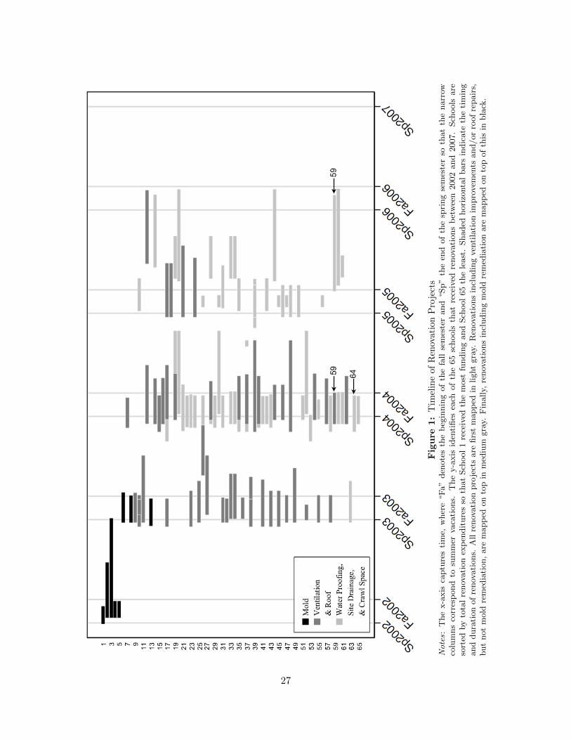
Fig

ure

1:

Tim

elin

eof

Ren

ovati

on

Pro

ject

sNotes:

The

x-a

xis

captu

res

tim

e,w

her

e“F

a”

den

ote

sth

eb

egin

nin

gof

the

fall

sem

este

rand

“Sp”

the

end

of

the

spri

ng

sem

este

rso

that

the

narr

owco

lum

ns

corr

esp

ond

tosu

mm

erva

cati

ons.

The

y-a

xis

iden

tifies

each

of

the

65

schools

that

rece

ived

renov

ati

ons

bet

wee

n2002

and

2007.

Sch

ools

are

sort

edby

tota

lre

nov

ati

on

exp

endit

ure

sso

that

Sch

ool

1re

ceiv

edth

em

ost

fundin

gand

Sch

ool

65

the

least

.Shaded

hori

zonta

lbars

indic

ate

the

tim

ing

and

dura

tion

of

renov

ati

ons.

All

renov

ati

on

pro

ject

sare

firs

tm

app

edin

light

gra

y.R

enov

ati

ons

incl

udin

gven

tila

tion

impro

vem

ents

and/or

roof

repair

s,but

not

mold

rem

edia

tion,

are

mapp

edon

top

inm

ediu

mgra

y.F

inally,

renov

ati

ons

incl

udin

gm

old

rem

edia

tion

are

mapp

edon

top

of

this

inbla

ck.

27

Fig

ure

2:

Dis

trib

uti

on

sof

Ren

ovati

on

Exp

end

itu

res

by

Pro

tect

Typ

eNotes:

The

num

ber

of

schools

wit

hpro

ject

sin

each

budget

cate

gory

isca

ptu

red

by

the

y-a

xis

and

the

level

of

exp

endit

ure

sby

the

x-a

xis

.P

roje

cts

are

colo

rco

ded

acc

ord

ing

toth

eva

riet

yof

oth

erpro

ject

typ

esb

eing

com

ple

ted

sim

ult

aneo

usl

y.L

egen

ds

use

the

follow

ing

short

hand

toid

enti

fypro

ject

s:“M

”-m

old

,“V

”-v

enti

lati

on,

“R

”-r

oof,

“W

”-w

ate

rpro

ofing,

“S”-s

ite

dra

inage,

“C

”-c

raw

lsp

ace

,and

“N

OID

”-n

ot

iden

tified

.Sum

mary

stati

stic

sare

giv

enfo

rse

ver

al

sam

ple

sw

her

e“N

”den

ote

sth

enum

ber

of

schools

inth

esa

mple

,“M

”th

em

ean

budget

,and

“SD

”th

est

andard

dev

iati

on.

The

his

togra

mfo

rven

tila

tion,

for

exam

ple

,sh

ows

that

thir

teen

schools

rece

ived

ven

tila

tion

impro

vem

ents

thatmay

hav

eb

een

acc

om

panie

dby

roof

repair

s,w

ate

rpro

ofing,

site

dra

inage,

or

craw

lsp

ace

renov

ati

ons

(+R,W

,S,C

).A

naddit

ional

thre

esc

hools

als

ore

ceiv

edm

old

rem

edia

tion

(+M

)and

anoth

ertw

oare

not

iden

tified

(+NO

ID).

28

Fig

ure

3:

Dis

trib

uti

on

sof

Mea

nC

lass

room

CO

2C

on

centr

ati

on

sA

cross

Sev

enStu

die

sNotes:

Thes

est

udie

sex

am

ine

elem

enta

rysc

hool

class

room

sin

(1)

Tex

as

(2)

Mic

hig

an,

(3)

Wash

ingto

nand

Idaho,

(4)

Rea

din

g,

Engla

nd,

(5)

Tex

as,

(6)

South

Caro

lina,

and

(7)

Uppsa

la,

Sw

eden

,re

spec

tivel

y.C

O2

ism

easu

red

inpart

sp

erm

illion

(ppm

).F

or

each

study,

and

when

available

,th

em

ean

of

all

mea

sure

dcl

ass

room

sis

dep

icte

dby

abla

ckdot,

one

standard

dev

iati

on

ab

ove

and

bel

owth

em

ean

by

the

med

ium

gra

yre

gio

n,

and

the

min

imum

and

maxim

um

by

the

extr

emes

of

the

light

gra

yre

gio

n.

The

ver

tica

lline

at

1,0

00ppm

corr

esp

onds

toth

em

axim

um

indoor

CO

2co

nce

ntr

ati

on

reco

mm

ended

by

ASH

RA

E.

29

Table 1: Estimates of the Impact of IAQ Renovations on TAKS Scores in Math and Reading

Variables All Mold Ventilation Roof Water Site Crawl

Panel A: Math Scores

after 0.021 0.165 ** 0.059 0.027 0.000 0.034 -0.118

(0.036) (0.065) (0.061) (0.040) (0.045) (0.064) (0.084)

Observations 37,286 19,238 21,018 23,387 23,692 21,094 19,886

Students 16,318 9,083 9,762 10,755 10,777 9,878 9,395

Panel B: Reading Scores

after 0.002 0.147 ** 0.098 ** 0.041 0.034 -0.003 -0.064

(0.032) (0.068) (0.043) (0.040) (0.037) (0.040) (0.045)

Observations 36,982 19,023 20,820 23,176 23,471 20,906 19,686

Students 16,171 8,978 9,668 10,646 10,671 9,782 9,298

Notes: Columns report regression results for different treatment classifications. For example, “Mold” clas-sify only projects that include mold remediation as treatment. In addition to after, all regressions includeclasssize, distexp, salary, year indicators, grade indicators, and student-school fixed effects. Robust stan-dard errors, clustered by school, are shown in parentheses below point estimates. Significance is denoted asfollows: *** p<0.01, ** p<0.05, * p<0.1.

30

Tab

le2:

Est

imate

sof

the

Impa

ctof

IAQ

Ren

ova

tion

son

TA

KS

Sco

res

Inco

rpora

tin

gP

roje

ctE

xpen

dit

ure

s

Mold

Ven

tila

tion

Roof

Wate

rSit

eC

raw

l

Vari

able

sA

llA

llN

oM

old

All

No

Mold

All

No

Mold

All

No

Mold

All

Panel

A:

Math

Sco

res

after

-0.2

60

**

-0.2

71

**

-0.4

39

**

-0.0

97

-0.0

76

-0.0

40

-0.0

12

-0.0

38

-0.0

39

-0.1

02

(0.1

08)

(0.1

09)

(0.1

82)

(0.0

74)

(0.0

78)

(0.0

57)

(0.0

56)

(0.0

87)

(0.1

81)

(0.2

85)

after*bu

dget

0.0

80

***

0.0

94

***

0.1

58

***

0.1

75

***

0.1

40

*0.0

32

**

-0.0

30

0.0

43

**

0.0

62

-0.0

37

(0.0

16)

(0.0

24)

(0.0

57)

(0.0

66)

(0.0

82)

(0.0

16)

(0.0

36)

(0.0

18)

(0.2

95)

(0.7

93)

TE

/M

ean

Budget†

0.1

54

***

0.0

49

0.0

35

0.0

16

0.0

09

-0.0

03

-0.0

37

0.0

15

-0.0

11

-0.1

16

(0.0

41)

(0.0

56)

(0.0

61)

(0.0

41)

(0.0

43)

(0.0

45)

(0.0

52)

(0.0

68)

(0.0

76)

(0.0

81)

TE

/M

ean

+1

sd†

0.2

76

***

0.1

74

***

0.1

80

**

0.0

82

**

0.0

55

0.0

47

-0.0

66

0.0

97

**

0.0

02

-0.1

21

(0.0

36)

(0.0

56)

(0.0

80)

(0.0

33)

(0.0

38)

(0.0

39)

(0.0

66)

(0.0

44)

(0.0

71)

(0.1

49)

Obse

rvati

ons

19,2

38

21,0

18

20,3

95

23,3

87

23,0

76

23,6

92

23,0

69

21,0

94

20,4

71

19,8

86

Stu

den

ts9,0

83

9,7

62

9,5

07

10,7

55

10,6

56

10,7

77

10,5

22

9,8

78

9,6

23

9,3

95

Panel

B:

Rea

din

gSco

res

after

-0.2

23

-0.1

01

-0.2

01

*-0

.065

-0.0

46

0.0

03

0.0

16

-0.0

73

0.0

01

-0.0

28

(0.1

34)

(0.0

67)

(0.1

20)

(0.0

57)

(0.0

53)

(0.0

45)

(0.0

45)

(0.0

49)

(0.0

84)

(0.1

18)

after*bu

dget

0.0

70

***

0.0

57

***

0.0

97

***

0.1

46

***

0.1

09

**

0.0

25

**

0.0

02

0.0

42

***

-0.1

28

-0.0

88

(0.0

20)

(0.0

14)

(0.0

35)

(0.0

40)

(0.0

41)

(0.0

12)

(0.0

32)

(0.0

10)

(0.1

96)

(0.2

33)

TE

/M

ean

Budget†

0.1

39

***

0.0

92

**

0.0

90

*0.0

30

0.0

19

0.0

31

0.0

18

-0.0

22

-0.0

56

-0.0

62

(0.0

42)

(0.0

43)

(0.0

46)

(0.0

43)

(0.0

44)

(0.0

38)

(0.0

43)

(0.0

41)

(0.0

47)

(0.0

45)

TE

/M

ean

+1

sd†

0.2

45

***

0.1

68

***

0.1

79

***

0.0

85

**

0.0

56

0.0

70

*0.0

19

0.0

58

-0.0

82

-0.0

73

*(0

.031)

(0.0

44)

(0.0

52)

(0.0

41)

(0.0

44)

(0.0

36)

(0.0

58)

(0.0

36)

(0.0

72)

(0.0

41)

Obse

rvati

ons

19,0

23

20,8

20

20,2

13

23,1

76

22,8

75

23,4

71

22,8

64

20,9

06

20,2

99

19,6

86

Stu

den

ts8,9

78

9,6

68

9,4

20

10,6

46

10,5

51

10,6

71

10,4

23

9,7

82

9,5

34

9,2

98

Notes:

Colu

mns

rep

ort

regre

ssio

nre

sult

sfo

rdiff

eren

ttr

eatm

ent

class

ifica

tions.

For

exam

ple

,“M

old

”cl

ass

ify

only

pro

ject

sth

at

incl

ude

mold

rem

edia

tion

as

trea

tmen

t.Sp

ecifi

cati

ons

lab

eled

“N

oM

old

”re

mov

em

old

pro

ject

sfr

om

the

trea

tmen

tgro

up.

Inaddit

ion

toafter

andafter∗bu

dget

,all

regre

ssio

ns

incl

udeclasssize,

distexp,sa

lary

,yea

rin

dic

ato

rs,

gra

de

indic

ato

rs,

and

studen

t-sc

hool

fixed

effec

ts.

Robust

standard

erro

rs,

clust

ered

by

school,

are

show

nin

pare

nth

eses

bel

owp

oin

tes

tim

ate

s.†C

om

bin

edtr

eatm

ent

effec

ts(“

TE

”),

wit

hst

andard

erro

rsb

elow

,are

rep

ort

edfo

r(i

)th

em

ean

budget

of

all

pro

ject

scl

ass

ified

as

“tr

eate

d”

inth

at

spec

ifica

tion

and

(ii)

the

mea

nbudget

plu

sone

standard

dev

iati

on.

Corr

esp

ondin

gbudget

stati

stic

sca

nb

efo

und

inF

igure

2.

Sig

nifi

cance

isden

ote

das

follow

s:***

p<

0.0

1,

**

p<

0.0

5,

*p<

0.1

.

31

Figure 4: Treatment Effects for Ventilation and Roof ProjectsNotes: Math and reading treatment effects for ventilation and roof projects are constructed using estimatesfrom columns labeled “No Mold” in Table 2. Treatment effects, measured in standard deviations, are illus-trated by a black line, with 90% confidence interval in gray. Graphs are split into four regions depending onthe sign and significance of treatment effects using the following notation: (1) negative and significant; (2)negative and insignificant; (3) positive and insignificant; and (4) positive and significant. Budget distribu-tions for projects classified as treated are overlaid. The number of schools falling into each budget categoryis given by the right hand side y-axis.

32

Table 3: Estimates of the Impact of IAQ Renovations on TAKS Scores One and Two Years Post-Renovations

Panel A: Math Scores Panel B: Reading Scores

Variables Mold Ventilation Roof Mold Ventilation Roof

after -0.247 * -0.244 ** -0.087 -0.188 -0.045 -0.050(0.129) (0.122) (0.077) (0.114) (0.059) (0.056)

after*budget 0.075 *** 0.089 *** 0.156 ** 0.062 *** 0.048 *** 0.137 ***(0.021) (0.026) (0.070) (0.017) (0.012) (0.042)

2yrs after 0.086 0.073 0.037 0.127 0.004 -0.015(0.128) (0.060) (0.062) (0.084) (0.035) (0.041)

2yrs after*budget -0.004 -0.003 -0.009 -0.003 0.002 0.004(0.006) (0.004) (0.009) (0.004) (0.003) (0.008)

p-value [0.784] [0.481] [0.570] [0.250] [0.689] [0.903]

Observations 19,238 20,725 22,622 19,023 20,529 22,409

Students 9083 9616 10357 8978 9523 10248

Notes: See Table 2. Two additional variables are added to Equation (1) to capture any differential effect ofrenovations across time post-renovations: (i) 2yrs after and (ii) 2yrs after*budget. Now, the coefficients onafter and after*budget capture the effect of renovations in the first year post-renovations and the combinationof all four treatment coefficients capture the effect of renovations in the second year post-renovations. P-values from joint significance tests of the two second year treatment variables are shown in brackets belowestimates.

33

Table 4: Linear Probability Estimates of the Impact of IAQ Renovations on the Probability ofPassing the TAKS

Mold Ventilation Roof

Variables All All No Mold All No Mold

Panel A: Math Scores

after 0.045 -0.067 -0.154 ** -0.012 -0.017(0.085) (0.044) (0.068) (0.023) (0.026)

after*budget -0.002 0.023 ** 0.054 *** 0.039 * 0.051 *(0.012) (0.011) (0.019) (0.021) (0.026)

TE/Mean Budget† 0.035 0.011 0.009 0.013 0.014(0.026) (0.021) (0.019) (0.015) (0.015)

TE/Mean + 1 sd† 0.032 * 0.042 0.058 *** 0.028 * 0.032 **(0.017) (0.025) (0.020) (0.015) (0.015)

Observations 19,238 21,018 20,395 23,387 23,076

Students 9,083 9,762 9,507 10,755 10,656

Panel B: Reading Scores

after 0.007 -0.063 -0.172 *** -0.021 -0.026(0.014) (0.040) (0.039) (0.019) (0.020)

after*budget 0.006 *** 0.025 ** 0.066 *** 0.054 *** 0.064 ***(0.002) (0.012) (0.010) (0.017) (0.023)

TE/Mean Budget† 0.038 *** 0.024 0.026 * 0.013 0.013(0.011) (0.017) (0.015) (0.015) (0.015)

TE/Mean + 1 sd† 0.048 *** 0.057 ** 0.087 *** 0.034 ** 0.034 *(0.012) (0.025) (0.014) (0.016) (0.017)

Observations 19,023 20,820 20,213 23,176 22,875

Students 8,978 9,668 9,420 10,646 10,551

Notes: See Table 2. Here, the dependent variable takes the value of 1 if student i passed the specified testin year y and takes the value of 0 otherwise. Explanatory variables are the same as those given in Equation(1).

34

Table 5: Estimates of the Impact of IAQ Renovations on School Attendance

Variables Mold Ventilation Roof Water Site Crawl

after -0.110 -0.016 -0.137 -0.083 0.028 -0.248(0.093) (0.290) (0.112) (0.073) (0.075) (0.200)

after*budget 0.035 *** -0.019 0.097 0.019 0.012 0.795(0.008) (0.073) (0.112) (0.018) (0.018) (0.481)

TE/Mean Budget† 0.068 -0.081 -0.074 -0.061 0.043 0.062(0.076) (0.098) (0.070) (0.066) (0.062) (0.074)

TE/Mean + 1 sd† 0.121 -0.106 -0.037 -0.031 0.066 0.159 *(0.075) (0.119) (0.072) (0.067) (0.056) (0.095)

Observations 39,976 43,356 48,630 48,989 44,090 41,810

Students 18,981 19,952 21,782 21,639 20,434 19,848

Notes: See Table 2. Results shown above are from versions of Equation (1) in which the dependent variableis school attendance rates, measured as a percentage from 0 to 100.

35

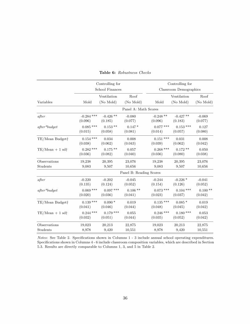
Table 6: Robustness Checks

Controlling for Controlling for

School Finances Classroom Demographics

Ventilation Roof Ventilation Roof

Variables Mold (No Mold) (No Mold) Mold (No Mold) (No Mold)

Panel A: Math Scores

after -0.284 *** -0.426 ** -0.080 -0.248 ** -0.427 ** -0.069(0.096) (0.185) (0.077) (0.096) (0.183) (0.077)

after*budget 0.085 *** 0.153 ** 0.147 * 0.077 *** 0.153 *** 0.127(0.015) (0.058) (0.081) (0.014) (0.057) (0.080)

TE/Mean Budget† 0.154 *** 0.034 0.008 0.151 *** 0.031 0.008(0.038) (0.062) (0.043) (0.039) (0.062) (0.042)

TE/Mean + 1 sd† 0.282 *** 0.175 ** 0.057 0.268 *** 0.172 ** 0.050(0.036) (0.082) (0.040) (0.036) (0.080) (0.038)

Observations 19,238 20,395 23,076 19,238 20,395 23,076

Students 9,083 9,507 10,656 9,083 9,507 10,656

Panel B: Reading Scores

after -0.220 -0.202 -0.045 -0.244 -0.226 * -0.041(0.135) (0.124) (0.052) (0.154) (0.126) (0.052)

after*budget 0.069 *** 0.097 *** 0.106 ** 0.073 *** 0.104 *** 0.100 **(0.020) (0.036) (0.041) (0.023) (0.037) (0.042)

TE/Mean Budget† 0.139 *** 0.090 * 0.019 0.135 *** 0.085 * 0.019(0.041) (0.046) (0.044) (0.048) (0.045) (0.042)

TE/Mean + 1 sd† 0.244 *** 0.179 *** 0.055 0.246 *** 0.180 *** 0.053(0.032) (0.051) (0.044) (0.035) (0.052) (0.042)

Observations 19,023 20,213 22,875 19,023 20,213 22,875

Students 8,978 9,420 10,551 8,978 9,420 10,551

Notes: See Table 2. Specifications shown in Columns 1 - 3 include annual school operating expenditures.Specifications shown in Columns 4 - 6 include classroom composition variables, which are described in Section5.3. Results are directly comparable to Columns 1, 3, and 5 in Table 2.

36