Publ ic   Interest  Energy  Research   (P IER)  Program  

FINAL  COLLABORATIVE  REPORT  

 

 

INDOOR ENVIRONMENTAL QUALITY AND HEATING, VENTILATING, AND AIR CONDITIONING SURVEY OF SMALL AND MEDIUM SIZE COMMERCIAL BUILDINGS 

 Field Study 

 

 

 Prepared for:  California Energy Commission 

Prepared by:  University of California at Davis and  Lawrence Berkeley National Lab 

 

 

 OCTOBER  2011

CEC ‐500 ‐2011 ‐043   

Prepared by:

Primary Author(s): Deborah Bennett Xiangmei (May) Wu Amber Trout

University of California, Davis Davis, CA 95616

Michael Apte David Faulkner Randy Maddalena Doug Sullivan

Lawrence Berkeley National Laboratory Berkeley, CA 94720

Contract Number: 500-02-023

Prepared for: California Energy Commission Marla Mueller Contract Manager Linda Spiegel Office Manager Energy Generation Research Office Laurie ten Hope Deputy Director ENERGY RESEARCH AND DEVELOPMENT DIVISION Robert P. Oglesby Executive Director and California Air Resources Board Ash Lashgari Contract Manager Research Division Eileen McCauley Manager Atmospheric Processes Research Section Research Division

  

 

 

 

  

DISCLAIMER This report was prepared as the result of work sponsored by the California Energy Commission. It does not necessarily represent the views of the Energy Commission, its employees or the State of California. The Energy Commission, the State of California, its employees, contractors and subcontractors make no warrant, express or implied, and assume no legal liability for the information in this report; nor does any party represent that the uses of this information will not infringe upon privately owned rights. This report has not been approved or disapproved by the California Energy Commission nor has the California Energy Commission passed upon the accuracy or adequacy of the information in this report.

 

LEGAL NOTICE 

This report was prepared as a result of work sponsored by the California Energy Commission (Energy Commission) and the Air Resources Board (ARB). It does not necessarily represent the views of the Energy Commission, ARB, their employees, or the State of California. The mention of commercial products, their source, or their use in connection with material reported herein is not to be construed as actual or implied endorsement of such products. The Energy Commission, ARB, the State of California, its employees, contractors, and subcontractors make no warranty, express or implied, and assume no legal liability for the information in this report; nor does any party represent that the use of this information will not infringe upon privately owned rights. This report has not been approved or disapproved by the Energy Commission or the ARB, nor has the Energy Commission or the ARB passed upon the accuracy or adequacy of this information in this report.  

 

i 

 

 

ACKNOWLEDGMENTS

The authors would like to thank all of the building operators and owners for allowing the project team to take measurements in their buildings for the study. The team also would like to acknowledge: 

• Additional members of the field staff, particularly Michael Powers, who completed all of the integrated measurements, as well as Candice Teague, Tom Liu, and Sebastian Cohn, who assisted with buildings early in the study.  

• Marion Russell and Mike Spears for laboratory analysis.  

• Tracy Armitage, Tamara Hennessy‐Burt, and Andrea Bergman for work done on the database development, data cleaning, and analysis of the inspection variables.  

• David Bonar and Colleen Philips for helping to prepare the report, and Rebecca Moran for support in various aspects of the project.  

• Bob Lee and Tom Piazza for their input into the project.  

• The valuable input and guidance from Martha Brook and G. William Pennington of the California Energy Commission, and Ash Lashgari, Peggy Jenkins, Eileen McCauley, and Tom Phillips of the California Air Resources Board, for both managing the project and for their valuable input. This project would not have been possible without the support and expertise of the researchers at these two agencies.  

• The Technical Advisory Group, including Jed Waldman, Steve Emmerich, Laura Kolb, Deborah Gold, and John Girman.   

• Bill Fisk for advice on determining building air exchange rates.  

• Petros Koutrakis, Mike Wolfson, and Steve Ferguson of the Harvard School of Public Health for providing additional cascading impactors to this project, and for their assistance in using the equipment.  

This research was funded by the California Energy Commission, Public Interest Energy Research Program through contract 500‐02‐023 with the California Air Resources Board. The Air Resources Board managed the research. The work at the University of California at Davis was supported through a subcontract from Air Resources Board Contract Number 06‐311. This report is submitted in fulfillment of that contract. The work at Lawrence Berkeley National Laboratory was supported through a subcontract from the University of California at Davis.  Additionally, all work conducted at Lawrence Berkeley National Laboratory is supported by the Director, Office of Science, Office of Basic Energy Sciences, of the U.S. Department of Energy under Contract No. DEAC02‐05CH11231. 

  

ii 

 

 

PREFACE

Public Interest Energy Research (PIER) Program supports public interest energy research and development that will help improve the quality of life in California by bringing environmentally safe, affordable, and reliable energy services and products to the marketplace. 

The PIER Program conducts public interest research, development, and demonstration (RD&D) projects to benefit California. The PIER Program strives to conduct the most promising public interest energy research by partnering with RD&D entities, including individuals, businesses, utilities, and public or private research institutions. PIER funding efforts are focused on the following RD&D program areas: 

• Buildings End‐Use Energy Efficiency 

• Energy Innovations Small Grants 

• Energy‐Related Environmental Research 

• Energy Systems Integration 

• Environmentally Preferred Advanced Generation 

• Industrial/Agricultural/Water End‐Use Energy Efficiency 

• Renewable Energy Technologies 

• Transportation 

For more information about the PIER Program, please visit the Energy Commission’s website at www.energy.ca.gov/research/ or contact the Energy Commission at 916‐327‐1551. 

The California Air Resources Board (ARB) carries out and funds research to reduce the health, environmental, and economic impacts of indoor and outdoor air pollution in California. This research involves four general program areas: 

• Health and Welfare Effects 

• Exposure Assessment 

• Technology Advancement and Pollution Prevention 

• Global Air Pollution 

For more information about the ARB Research Program, please see ARB’s website at: www.arb.ca.gov/research/research.htm, or contact ARB’s Research Division at 916‐445‐0753. 

For more information about ARB’s Indoor Exposure Assessment Program please visit the website at: www.arb.ca.gov/research/indoor/indoor.htm. 

Indoor Environmental Quality and Heating, Ventilating, and Air Conditioning Survey of Small and Medium Size Commercial Buildings: Field Study is the final report for the project, Contract Number 500‐02‐023 and ARB Contract Number 06‐311, conducted by University of California, Davis. The information from this project contributes to PIER’s Energy‐Related Environmental Research Program. 

iii 

 

 

 ABSTRACT 

Ninety‐six percent of commercial buildings in the United States are small‐ to medium‐sized, use nearly 18 percent of the country’s energy, and shelter a large proportion of population, thus underlining the importance of understanding the relationship between ventilation, energy use, and air quality. This field study of 37 such buildings throughout California obtained information on all aspects of ventilation and levels of indoor air pollutants. The study included seven retail establishments: five restaurants; eight offices; two gas stations, hair salons, healthcare facilities, grocery stores, dental offices, and fitness gyms; and five other buildings.  

Sixteen (43 percent) of the buildings were not designed to or did not provide mechanically supplied outdoor ventilation air. In some cases the air handling unit was a residential rather than a commercial model, thereby failing to meet applicable ventilation standards. Low‐efficiency air filters were frequently observed. The air exchange rate averaged 1.6 with a standard deviation of 1.7 exchanges per hour and was similar between buildings with and without mechanically supplied outdoor air, indicating that buildings have significant leakage, in contrast to California homes. Compared against Title 24 standards, healthcare establishments, gyms, offices, hair salons, and retail stores were ventilated below the required rates, not meeting Title 24 ventilation requirements; restaurants and gas stations had rates above the standard, meeting ventilation requirements.  

Indoor/outdoor ratios of ultrafine particulate matter and particulate matter smaller than 2.5 microns were less than 1.0 in most buildings; exceptions were restaurants, hair salons, and dental offices, which have known indoor sources. The average black carbon ratio was 0.72, indicating that the building shell and heating, ventilation, and air conditioning system provided partial protection from outdoor particulates. Aldehydes and volatile organic compounds were measured. The majority of buildings had formaldehyde levels above the Office of Environmental Health Hazard Assessment 8‐hour reference exposure level.  

Recommendations based on this study’s finding are: (1) require a mandatory inspection to confirm that appropriate mechanically supplied air is supplied; (2) increase formaldehyde source control; and (3) require increased air filter efficiencies. 

 

Keywords: Small and medium commercial buildings, indoor air quality, ventilation, air contaminant exposure guidelines, air exchange rate, carbon monoxide, building envelope tightness, exhaust fans, formaldehyde, indoor air contaminant emission rates, indoor air contaminant sources, indoor air quality, mechanical ventilation systems, natural ventilation, nitrogen dioxide, particulate matter, ventilation standards, volatile organic compounds, windows 

iv 

 

 

Please use the following citation for this report: 

Bennett, Deborah, Michael Apte, Xiangmei (May) Wu, Amber Trout, David Faulkner, Randy Maddalena, and Doug Sullivan (University of California Davis). 2011. Indoor Environmental Quality and Heating, Ventilating, and Air Conditioning Survey of Small and Medium Size Commercial Buildings: Field Study. California Energy Commission. CEC‐500‐2011‐043. 

v 

 

 

vi 

 

 

TABLE OF CONTENTS 

ACKNOWLEDGMENTS ....................................................................................................................... ii 

PREFACE .................................................................................................................................................. iii 

ABSTRACT .............................................................................................................................................. iv 

TABLE OF CONTENTS ........................................................................................................................ vii 

LIST OF FIGURES .................................................................................................................................... x 

LIST OF TABLES ................................................................................................................................... xii 

EXECUTIVE SUMMARY ........................................................................................................................ 1 

CHAPTER 1: Introduction ....................................................................................................................... 7 

Study Objectives ..................................................................................................................................... 9 

Background ........................................................................................................................................... 10 

Available Research on Commercial Buildings............................................................................. 10 

Relevance of Pollutant Exposure Issues to Commercial Buildings .......................................... 15 

Needs and Uses for Data................................................................................................................. 16 

Relevant Standards and Guidelines for Comparison ................................................................. 18 

CHAPTER 2: Methods ............................................................................................................................ 32 

Building Selection ................................................................................................................................ 32 

Distribution of Buildings in California ......................................................................................... 32 

Distributional Goals ......................................................................................................................... 34 

Building Selection Procedures ....................................................................................................... 35 

Heating, Ventilation, and Air‐Conditioning Systems ..................................................................... 36 

Characterization of Physical Plant: Maintenance and Operation of Building, Focus on HVAC and Air Filtration Systems ................................................................................................. 36 

Measurements of Air Exchange ..................................................................................................... 41 

Carbon Dioxide Measurements ..................................................................................................... 52 

Temperature and Relative Humidity ............................................................................................ 52 

Indoor Air Quality ............................................................................................................................... 53 

Criteria Air Pollutants ..................................................................................................................... 53 vii 

 

 

Toxic Air Contaminants .................................................................................................................. 55 

History of Moisture and IAQ/Ventilation Problems ................................................................... 57 

Particle Infiltration ........................................................................................................................... 58 

Data Analysis ........................................................................................................................................ 60 

Characterization of Physical Plant: Maintenance and Operation of Building, Focus on HVAC and Air Filtration Systems ................................................................................................. 60 

Building Ventilation ........................................................................................................................ 62 

Criteria Air Pollutants ..................................................................................................................... 64 

Toxic Air Contaminants .................................................................................................................. 64 

Particle Infiltration ........................................................................................................................... 66 

CHAPTER 3: Results and Discussion ................................................................................................. 68 

Building Recruitment .......................................................................................................................... 68 

Distribution of Buildings ................................................................................................................ 69 

Building Descriptions ...................................................................................................................... 70 

Heating, Ventilation, and Air Conditioning Systems ..................................................................... 72 

Characterization of Physical Plant: Maintenance and Operation of Building, with a Focus on HVAC and Air Filtration Systems ........................................................................................... 72 

Measurements of Air Exchange ..................................................................................................... 86 

Carbon Dioxide Measurements ................................................................................................... 105 

Temperature and Relative Humidity .......................................................................................... 107 

Indoor Air Quality ............................................................................................................................. 110 

Criteria Air Pollutants ................................................................................................................... 110 

QA/QC Results for Integrated PM Measures ............................................................................. 123 

Ultrafine Particle Counts............................................................................................................... 124 

Toxic Air Contaminants ................................................................................................................ 129 

History of Moisture and IAQ/Ventilation Problems ................................................................. 172 

Particle Infiltration ......................................................................................................................... 176 

CHAPTER 4: Conclusions and Recommendations ......................................................................... 185 

viii 

 

 

Conclusions ......................................................................................................................................... 185 

Objective 1: Obtain data on SMCB building characteristics, operation and maintenance of their HVAC, and air filtration systems. ...................................................................................... 185 

Objective 2: Recognizing that measurement of air flow can be problematic, field data on the design and performance parameters of HVAC and air filtration systems in SMCB were to be obtained. ..................................................................................................................................... 186 

Objective 3: Obtain data on indoor pollutant levels, especially toxic air contaminants, and potential pollutant sources in a variety of SMCB. To the extent feasible, determine the moisture‐related history and IAQ complaint history. .............................................................. 188 

Objective 4: Measure particulate matter inside and outside of buildings, to estimate penetration rates for particulate matter in a variety of SMCB. ............................................... 189 

Recommendations .............................................................................................................................. 190 

Inspection Procedure and Maintenance ..................................................................................... 190 

Indoor Air Quality ......................................................................................................................... 191 

References ............................................................................................................................................... 193 

Glossary .................................................................................................................................................. 212 

APPENDICES ........................................................................................................................................ 215 

 

Appendix A: Inspection, Walk‐through, and Questionnaire Data 

Appendix B: Building Descriptions for all Buildings 

Appendix C: Summary Statistics for Each Building 

Appendix D: Air Exchange Summary for Each Building 

Appendix E: Met One Results for Each Building 

Appendix F: Ultrafine Results for Each Building 

Appendix G: VOC Concentrations, Indoor/Outdoor Ratios, Indoor/Outdoor Differences, and Building Source Strengths 

Appendix H: Aethalometer Results for Each Building 

ix 

 

 

LIST OF FIGURES

Figure 1: ASHRAE Summer and Winter Comfort Zones, as Defined in  ASHRAE 55‐2004, Figure 5.2.1.1 ......................................................................................................................................................... 21 

Figure 2: Diagram of the Tracer Gas Airflow Measurement System (TRAMS) .............................. 48 

Figure 3: Air Handling Unit Housing Condition ................................................................................ 73 

Figure 4: Air Handling Unit Component Condition ........................................................................... 73 

Figure 5: Air Distribution Ductwork Condition .................................................................................. 74 

Figure 6:  Particulate Filtration Systems Condition ............................................................................ 74 

Figure 7:  Control System Condition ..................................................................................................... 75 

Figure 8: Fraction of Buildings With No Outdoor Air by Building Characteristics ....................... 77 

Figure 9: Overall Condition by Building Size ...................................................................................... 78 

Figure 10: Overall Condition by Building Age .................................................................................... 78 

Figure 11: MERV Ratings Collected from HVAC Filters Inspected at SMCB ................................. 79 

Figure 12: The Fraction of Buildings Falling Into Each Maintenance Category.............................. 80 

Figure 13: Distribution of the Maintenance Category Among Small Buildings and Among  Buildings That Fell Into Either the Medium or Medium/Large Category ....................................... 81 

Figure 14: Distribution of Months Between Inspections .................................................................... 82 

Figure 15: The Distribution of the Frequency of Contractor Inspections  for Buildings in Each of the Three Maintenance Categories ........................................................................................................ 83 

Figure 16: Distribution of the Number of Systems Inspected for Buildings in Each Maintenance Category .................................................................................................................................................... 84 

Figure 17: The Distribution of the Overall Inspection Result for Buildings  in Each of the Five Building Maintenance Categories .......................................................................................................... 86 

Figure 18: Distributions of Whole‐Building Ventilation Rates .......................................................... 92 

Figure 19: Scatter Plot of Ventilation Rates Measured by  PFT Steady‐State and Tracer Decay Method....................................................................................................................................................... 93 

Figure 20: Air Exchange Rate Versus Year Built .................................................................................. 96 

Figure 21: Air Exchange Rate by Building Location ........................................................................... 97 

Figure 22: Air Exchange Rate by Building Size ................................................................................... 97 

x 

 

 

Figure 23: Air Exchange Rate by Building Use .................................................................................... 98 

Figure 24: Air Exchange Rate Vs. Ventilation Mechanism ............................................................... 100 

Figure 25: Comparison of Air Exchange Rates to Title 24 by Person ............................................. 101 

Figure 26: Comparison of Air Exchange Rates to Title 24 by Area ................................................. 102 

Figure 27: Comparison of Air Exchange Rates to ASHRAE 62.1 .................................................... 103 

Figure 28: Distribution of Indoor Concentrations  of Particulate Matter by Building Type ....... 113 

Figure 29: Distribution of Indoor PM2.5 Concentrations by Building Type…...…………………120 

Figure 30: Distribution of Indoor PM10 Concentrations by Building Type………………………120 

Figure 31: Comparison Bewteen  PM10 Concentrations Collected by Filter and the Sum of PM2.5 Concentrations Collected By Filter and PM2.5‐10 Concentrations Collected by PUF…………..…124 

Figure 32: Distribution of Indoor Ultrafine Particle Count by Building Type .............................. 126 

Figure 33: Distribution of Indoor VOC Concentrations ................................................................... 133 

Figure 34: Indoor Concentrations of Phenol by Building Type ....................................................... 141 

Figure 35: Indoor Concentrations of Diethylphthalate by Building Type ..................................... 142 

Figure 36: Indoor Concentrations of D‐5 Siloxane by Building Type ............................................. 142 

Figure 37: Indoor Concentrations of Ethylbenzene by Building Type ........................................... 143 

Figure 38: Indoor Concentrations of m/p‐Xylene by Building Type .............................................. 143 

Figure 39: Indoor Concentrations of o‐Xylene by Building Type ................................................... 144 

Figure 40: Indoor Concentrations of Benzene by Building Type………………………………….144 

Figure 41: Indoor Concentrations of Acetaldehyde by Building Type……………………...……145 

Figure 42: Indoor Concentrations of Chloroform by Building Type .............................................. 146 

Figure 43: Indoor Concentrations of PCE by Building Type ........................................................... 146 

Figure 44: Indoor Concentrations of Naphthalene by Building Type ............................................ 147 

Figure 45: Indoor Concentrations of TXIB by Building Type .......................................................... 147 

Figure 46: Indoor Concentrations of Acetone by Building Type..................................................... 148 

Figure 47: Indoor Concentrations of Formaldehyde by Building Type ......................................... 148 

Figure 48: Distribution of Formaldehyde Concentrations if Ventilation Rates in All Buildings Were Equal to the Rate Required by Title 24, Per Area .................................................................... 158 

xi 

 

 

Figure 49: Indoor Formaldehyde Concentrations by Building Type With and Without (A) Any Carpet Present and (B) Carpet as Primary Flooring ......................................................................... 160 

Figure 50: Air Exchange Rate in Buildings With and Without a Water Damage Issue……….173 

Figure 51: Overall Building Inspection Score in Buildings With and Without a Water Damage Issue……………………………………………………………………………………………….…….173 

Figure 52: Comparison of Indoor/Outdoor Ratio of Black Carbon by Building Ventilation Condition ................................................................................................................................................. 179 

Figure 53: Comparison of Indoor/Outdoor Ratio of Black Carbon by Building Ventilation Condition, A. Using Street‐level Black Carbon Concentrations, and B. Using Rooftop Carbon Concentrations ........................................................................................................................................ 180 

Figure 54: Comparison of Indoor/outdoor Ratio of Black Carbon by Building Type .................. 181 

Figure 55: Indoor/Outdoor Ratio of Black Carbon vs. Building Age .............................................. 182 

Figure 56: Particle Penetration Values Versus MERV Filter Ratings .............................................. 183 

 

LIST OF TABLES

Table 1: Minimum Ventilation Rates as Listed in Title 24, Table 121A ............................................ 19 

Table 2: ASHRAE 62.1 Ventilation Rates .............................................................................................. 19 

Table 3: Compounds Monitored, Potential Indoor Sources,  and Potential Health Effects .......... 23 

Table 4: OSHA and Cal/OSHA Permissible Exposure Limits (PELs) ............................................... 28 

Table 5: OEHHA Reference Exposure Levels (RELs) ......................................................................... 29 

Table 6: VOC Toxicity Data Available in U.S. EPA Integrated Risk Information System (IRIS) .. 30 

Table 7: No Significant Risk Level (NSRL) for Carcinogen or Maximum Allowable Dose Level (MADL) for Reproductive Toxicants Required by California Proposition 65 for the Chemicals Measured in This Study .......................................................................................................................... 31 

Table 8: Distributions of Building Types in Previous  Commercial Building Surveys .................. 33 

Table 9: Number of Buildings Interested in Learning More About the Field Survey .................... 35 

Table 10: List of Questions in Building Inspection .............................................................................. 37 

Table 11: ASHRAE Standard Testing Method 52.2‐2007 MERV Table ............................................ 41 

Table 12: Whole Building Ventilation ................................................................................................... 49 

Table 13: Mechanical Outside Air Supply Flow Measurement ......................................................... 51 xii 

 

 

Table 14: Target List of Volatile Organic Chemicals Quantified in the SMCB Study .................... 57 

Table 15: SMCB Study Building Recruitment Statistics for Establishments  Identified in the SMCB Phone Survey ................................................................................................................................ 68 

Table 16: List of Buildings That Participated in Study Detailing  Business Type, Location, and Building Size ............................................................................................................................................. 71 

Table 17: Reported Frequencies of Selected System Maintenance Activities in the BASE Study . 83 

Table 18: Number of Buildings Reporting That the Specified System Was Inspected  on the Most Recent Inspection, Out of the 14 Buildings Reporting ........................................................................ 84 

Table 19: Distribution of Building Ventilation Rate ............................................................................ 90 

Table 20: Results of Multiple Regression Analysis for Ventilation Rate Per Area ......................... 99 

Table 21: Buildings Significantly Higher or Lower Than Title 24 Ventilation Rates by Area ..... 104 

Table 22: Buildings Significantly Higher or Lower Than Title 24 Ventilation Rates by Person . 105 

Table 23: Summary Statistics for Carbon Dioxide ............................................................................. 105 

Table 24: Summary Statistics for the 95th Percentile of the CO2 Indoor/Outdoor  Difference Across the Buildings .............................................................................................................................. 106 

Table 25: Summary Statistics for Temperature .................................................................................. 108 

Table 26: Summary Statistics for Relative Humidity ........................................................................ 108 

Table 27: Distribution of Indoor Particulate Matter Concentrations .............................................. 112 

Table 28: Indoor/Outdoor Ratios of Particulate Matter  vs. Building Type for Each Particle Size Fraction .................................................................................................................................................... 114 

Table 29: Adjustments Made to Met One Concentrations ............................................................... 116 

Table 30: Distribution of Indoor and Outdoor PM2.5 Concentrations  and Indoor/Outdoor Ratio for All Buildings and by Building Type .............................................................................................. 118 

Table 31: Distribution of Indoor and Outdoor PM10 Concentrations  and Indoor/outdoor Ratio for All Buildings and by Building Type .............................................................................................. 119 

Table 32: Number of Buildings in Each I/O Ratio Range for PM2.5 by Building Type ................. 121 

Table 33: Number of Buildings in Each I/O Ratio Range for PM10 by Building Type .................. 121 

Table 34: Cross Frequency for PM2.5: Daytime Average Indoor Concentration  vs. Indoor/Outdoor Ratio ............................................................................................................................ 121 

Table 35: PM2.5 Concentrations in Previous Studies of Commercial Buildings ............................. 122 

xiii 

 

 

Table 36: Comparison Between PM Concentration in the SMCB Study and the BASE Study ... 123 

Table 37: Distribution of Ultrafine Particle Count ............................................................................. 125 

Table 38: Indoor/Outdoor Ratio of Ultrafine Particles vs. Building Type ..................................... 126 

Table 39: Cross Frequency for Ultrafine Particles: Daytime Average Indoor Count vs. Indoor/Outdoor Ratio ............................................................................................................................ 127 

Table 40: Ultrafine Particle Counts Reported in Other Studies ....................................................... 128 

Table 41: Results of Co‐location of Ultrafine Monitors ..................................................................... 129 

Table 42: Methylene Chloride Concentration (μg/m3) With Potential Contamination Issues .... 131 

Table 43: Distribution of Indoor Concentrations of VOCs Across All Samples ............................ 134 

Table 44: Distribution of Indoor Concentrations of VOCs Across All Buildings ......................... 135 

Table 45: Distribution of Outdoor Concentrations of VOCs Across All Buildings ...................... 136 

Table 46: Distribution of Indoor/Outdoor Concentration Ratios of VOCs Across All Buildings .................................................................................................................................................................. 137 

Table 47: Distribution of Indoor/Outdoor Concentration Differences of VOCs Across All Buildings ................................................................................................................................................. 138 

Table 48: Extremely High VOC Concentrations Observed in SMCBs ............................................ 139 

Table 49: Distribution of Building Source Strength of VOCs Across All Buildings ..................... 151 

Table 50: Distribution of Building Source Strength of VOCs per Area Across All Buildings ..... 152 

Table 51: Number of Buildings with Indoor Concentrations Exceeding OEHHA RELs…...…..152 

Table 52: Comparison of Indoor Concentrations with U.S. EPA Inhalation Risk Level Concentrations for Carcinogens………………………………………………………………………152 

Table 53: Buildings with VOC Concentrations Above the Requirement in Proposition 65 ........ 154 

Table 54: Comparison of Indoor VOC Concentrations (μg/m3) With Other Studies ................... 157 

Table 55: Impact of the Presence of Carpet and Wood Furniture  on Indoor Formaldehyde Concentration ......................................................................................................................................... 159 

Table 56: Pearson Correlation Coefficients Between Indoor VOC Concentrations ...................... 163 

Table 57: Loadings of the First Trial of Factor Analysis ................................................................... 165 

Table 58: Rotated Factor Pattern (Standardized Regression Coefficients) ..................................... 166 

Table 59: Parameters Related to Chemical Analysis for VOCs and Aldehydes ............................ 167 

xiv 

 

 

Table 60: Quality Assurance Results for Analysis and Sample Handling of VOCs……………..168 

Table 61: Assurance Measures for Sample Collection………………………………….…………..169 

Table 62: Collection Efficiency for VOCs…………………………………………………...………..170 

Table 63: Frequency of Buildings with Past or Current Water Damage ........................................ 173 

Table 64: Number of Buildings with Complaints .............................................................................. 175 

Table 65: Percentage of Buildings with Complaints ......................................................................... 176 

Table 66: Percentage of Buildings with Complaints from SMCB Phone Survey .......................... 176 

Table 67: Distribution of Indoor/Outdoor Ratios of Black Carbon ................................................. 178 

xv 

 

 

xvi 

 

  

 

 

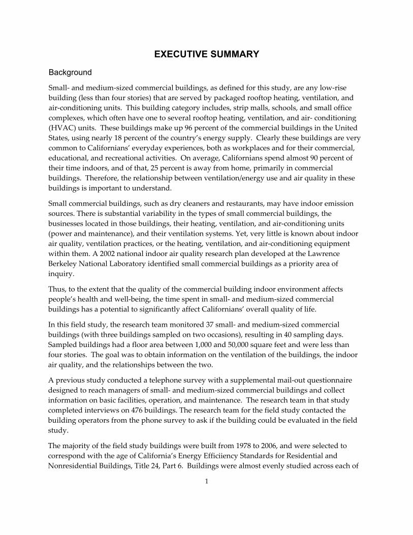
EXECUTIVE SUMMARY

Background

Small‐ and medium‐sized commercial buildings, as defined for this study, are any low‐rise building (less than four stories) that are served by packaged rooftop heating, ventilation, and air‐conditioning units.  This building category includes, strip malls, schools, and small office complexes, which often have one to several rooftop heating, ventilation, and air‐ conditioning (HVAC) units.  These buildings make up 96 percent of the commercial buildings in the United States, using nearly 18 percent of the country’s energy supply.  Clearly these buildings are very common to Californians’ everyday experiences, both as workplaces and for their commercial, educational, and recreational activities.  On average, Californians spend almost 90 percent of their time indoors, and of that, 25 percent is away from home, primarily in commercial buildings.  Therefore, the relationship between ventilation/energy use and air quality in these buildings is important to understand.  

Small commercial buildings, such as dry cleaners and restaurants, may have indoor emission sources. There is substantial variability in the types of small commercial buildings, the businesses located in those buildings, their heating, ventilation, and air‐conditioning units (power and maintenance), and their ventilation systems. Yet, very little is known about indoor air quality, ventilation practices, or the heating, ventilation, and air‐conditioning equipment within them. A 2002 national indoor air quality research plan developed at the Lawrence Berkeley National Laboratory identified small commercial buildings as a priority area of inquiry. 

Thus, to the extent that the quality of the commercial building indoor environment affects people’s health and well‐being, the time spent in small‐ and medium‐sized commercial buildings has a potential to significantly affect Californians’ overall quality of life.   

In this field study, the research team monitored 37 small‐ and medium‐sized commercial buildings (with three buildings sampled on two occasions), resulting in 40 sampling days.  Sampled buildings had a floor area between 1,000 and 50,000 square feet and were less than four stories.  The goal was to obtain information on the ventilation of the buildings, the indoor air quality, and the relationships between the two.  

A previous study conducted a telephone survey with a supplemental mail‐out questionnaire designed to reach managers of small‐ and medium‐sized commercial buildings and collect information on basic facilities, operation, and maintenance.  The research team in that study completed interviews on 476 buildings. The research team for the field study contacted the building operators from the phone survey to ask if the building could be evaluated in the field study. 

The majority of the field study buildings were built from 1978 to 2006, and were selected to correspond with the age of California’s Energy Efficiiency Standards for Residential and Nonresidential Buildings, Title 24, Part 6.  Buildings were almost evenly studied across each of 

1 

 

 

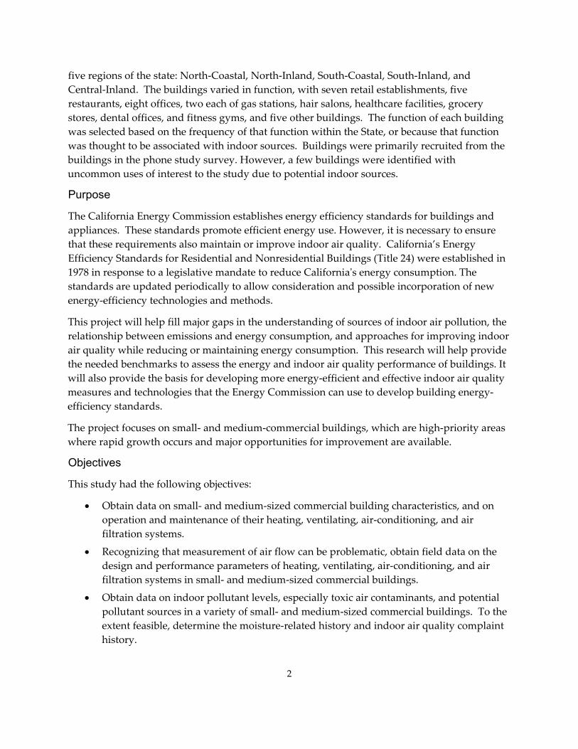
five regions of the state: North‐Coastal, North‐Inland, South‐Coastal, South‐Inland, and Central‐Inland.  The buildings varied in function, with seven retail establishments, five restaurants, eight offices, two each of gas stations, hair salons, healthcare facilities, grocery stores, dental offices, and fitness gyms, and five other buildings.  The function of each building was selected based on the frequency of that function within the State, or because that function was thought to be associated with indoor sources.  Buildings were primarily recruited from the buildings in the phone study survey. However, a few buildings were identified with uncommon uses of interest to the study due to potential indoor sources.   

Purpose

The California Energy Commission establishes energy efficiency standards for buildings and appliances.  These standards promote efficient energy use. However, it is necessary to ensure that these requirements also maintain or improve indoor air quality.  California’s Energy Efficiency Standards for Residential and Nonresidential Buildings (Title 24) were established in 1978 in response to a legislative mandate to reduce Californiaʹs energy consumption. The standards are updated periodically to allow consideration and possible incorporation of new energy‐efficiency technologies and methods.  

This project will help fill major gaps in the understanding of sources of indoor air pollution, the relationship between emissions and energy consumption, and approaches for improving indoor air quality while reducing or maintaining energy consumption.  This research will help provide the needed benchmarks to assess the energy and indoor air quality performance of buildings. It will also provide the basis for developing more energy‐efficient and effective indoor air quality measures and technologies that the Energy Commission can use to develop building energy‐efficiency standards. 

The project focuses on small‐ and medium‐commercial buildings, which are high‐priority areas where rapid growth occurs and major opportunities for improvement are available.   

Objectives

This study had the following objectives: 

• Obtain data on small‐ and medium‐sized commercial building characteristics, and on operation and maintenance of their heating, ventilating, air‐conditioning, and air filtration systems. 

• Recognizing that measurement of air flow can be problematic, obtain field data on the design and performance parameters of heating, ventilating, air‐conditioning, and air filtration systems in small‐ and medium‐sized commercial buildings. 

• Obtain data on indoor pollutant levels, especially toxic air contaminants, and potential pollutant sources in a variety of small‐ and medium‐sized commercial buildings.  To the extent feasible, determine the moisture‐related history and indoor air quality complaint history.   

2 

 

 

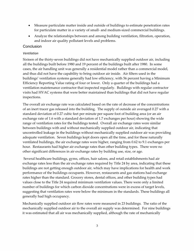
• Measure particulate matter inside and outside of buildings to estimate penetration rates for particulate matter in a variety of small‐ and medium‐sized commercial buildings. 

• Analyze the relationships between and among building ventilation, filtration, operation, and indoor air quality pollutant levels and problems. 

Conclusion

Ventilation 

Sixteen of the thirty‐seven buildings did not have mechanically supplied outdoor air, including all the buildings built before 1980 and 19 percent of the buildings built after 1980.  In some cases, the air handling unit was generally a residential model rather than a commercial model, and thus did not have the capability to bring outdoor air inside.  Air filters used in the buildings’ ventilation systems generally had low efficiency, with 56 percent having a Minimum Efficiency Reporting Value rating of four or lower.  Only a quarter of the buildings had a ventilation maintenance contractor that inspected regularly.  Buildings with regular contractor visits had HVAC systems that were better maintained than buildings that did not have regular inspections. 

The overall air exchange rate was calculated based on the rate of decrease of the concentrations of an inert tracer gas released into the building.  The supply of outside air averaged 0.27 with a standard deviation of 0.27 cubic feet per minute per square foot of building area (or an air exchange rate of 1.6 with a standard deviation of 1.7 exchanges per hour) showing the wide range of ventilation rates for the buildings tested.  Overall air exchange rates were similar between buildings with and without mechanically supplied outdoor air, indicating that uncontrolled leakage in the buildings without mechanically supplied outdoor air was providing adequate ventilation.  Seven buildings kept doors open all the time, and for these naturally ventilated buildings, the air exchange rates were higher, ranging from 0.62 to 9.1 exchanges per hour.  Restaurants had higher air exchange rates than other building types.  There were no other significant differences in air exchange rates by building use, size, or age.   

 Several healthcare buildings, gyms, offices, hair salons, and retail establishments had air exchange rates less than the air exchange rates required by Title 24 by area, indicating that these buildings are not getting enough outdoor air, which may have implications for health and work performance of the buildings occupants. However, restaurants and gas stations had exchange rates higher than the standard. Grocery stores, dental offices, and other building types had values close to the Title 24 required minimum ventilation values. There were only a limited number of buildings for which carbon dioxide concentrations were in excess of target levels, suggesting that ventilation rates were below the minimum in the standards. These buildings all generally had high occupancy. 

Mechanically supplied outdoor air flow rates were measured in 23 buildings.  The ratio of the mechanically supplied outdoor air to the overall air supply was determined.  For nine buildings it was estimated that all air was mechanically supplied, although the rate of mechanically 

3 

 

 

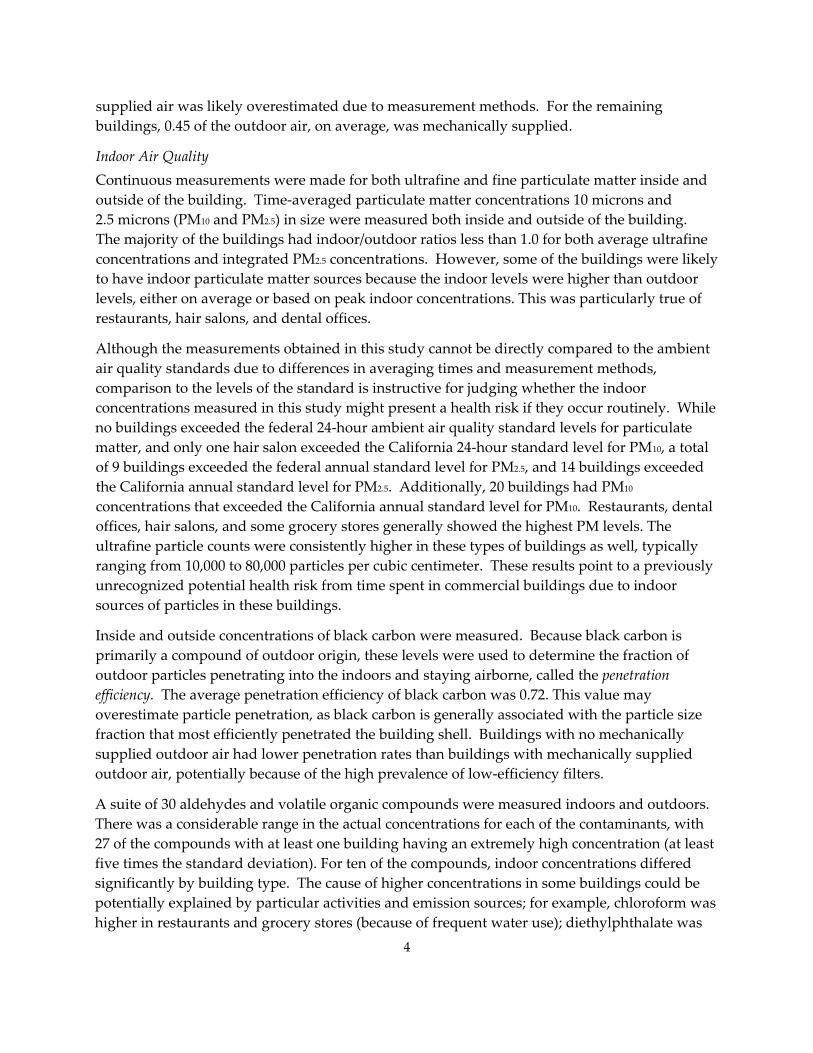
supplied air was likely overestimated due to measurement methods.  For the remaining buildings, 0.45 of the outdoor air, on average, was mechanically supplied. 

Indoor Air Quality Continuous measurements were made for both ultrafine and fine particulate matter inside and outside of the building.  Time‐averaged particulate matter concentrations 10 microns and 2.5 microns (PM10 and PM2.5) in size were measured both inside and outside of the building.  The majority of the buildings had indoor/outdoor ratios less than 1.0 for both average ultrafine concentrations and integrated PM2.5 concentrations.  However, some of the buildings were likely to have indoor particulate matter sources because the indoor levels were higher than outdoor levels, either on average or based on peak indoor concentrations. This was particularly true of restaurants, hair salons, and dental offices.  

Although the measurements obtained in this study cannot be directly compared to the ambient air quality standards due to differences in averaging times and measurement methods, comparison to the levels of the standard is instructive for judging whether the indoor concentrations measured in this study might present a health risk if they occur routinely.  While no buildings exceeded the federal 24‐hour ambient air quality standard levels for particulate matter, and only one hair salon exceeded the California 24‐hour standard level for PM10, a total of 9 buildings exceeded the federal annual standard level for PM2.5, and 14 buildings exceeded the California annual standard level for PM2.5.  Additionally, 20 buildings had PM10 concentrations that exceeded the California annual standard level for PM10.  Restaurants, dental offices, hair salons, and some grocery stores generally showed the highest PM levels. The ultrafine particle counts were consistently higher in these types of buildings as well, typically ranging from 10,000 to 80,000 particles per cubic centimeter.  These results point to a previously unrecognized potential health risk from time spent in commercial buildings due to indoor sources of particles in these buildings. 

Inside and outside concentrations of black carbon were measured.  Because black carbon is primarily a compound of outdoor origin, these levels were used to determine the fraction of outdoor particles penetrating into the indoors and staying airborne, called the penetration efficiency.  The average penetration efficiency of black carbon was 0.72. This value may overestimate particle penetration, as black carbon is generally associated with the particle size fraction that most efficiently penetrated the building shell.  Buildings with no mechanically supplied outdoor air had lower penetration rates than buildings with mechanically supplied outdoor air, potentially because of the high prevalence of low‐efficiency filters. 

A suite of 30 aldehydes and volatile organic compounds were measured indoors and outdoors.  There was a considerable range in the actual concentrations for each of the contaminants, with 27 of the compounds with at least one building having an extremely high concentration (at least five times the standard deviation). For ten of the compounds, indoor concentrations differed significantly by building type.  The cause of higher concentrations in some buildings could be potentially explained by particular activities and emission sources; for example, chloroform was higher in restaurants and grocery stores (because of frequent water use); diethylphthalate was 

4 

 

 

higher in dental offices, healthcare establishments, hair salons, and gyms (because of frequent cleaning and personal care product use); and m/p‐xylene was higher at gas stations (because it is a volatile component of gasoline). 

The majority of buildings (95 percent) had measured formaldehyde levels above the Office of Environmental Health Hazard Assessment chronic reference exposure level, indicating the need for building products and furnishings that emit less formaldehyde.  Three of the buildings had formaldehyde levels exceeding the Office of Environmental Health Hazard Assessment acute reference exposure level.  In terms of exceeding cancer risk levels, 100 percent of the buildings exceeded the one‐in‐a‐million concentration for benzene, formaldehyde, acetaldehyde, and chloroform.  At the 1‐in‐100,000 risk concentration level, these numbers dropped to 10 percent of the buildings exceeding for benzene, 82.5 percent of the buildings exceeding for acetaldehyde, and 35 percent of the buildings exceeding for chloroform.  All of the buildings exceeded the 1‐in‐100,000 risk level concentration for formaldehyde, with 87.5 percent exceeding the 1‐in‐10,000 risk level for this compound. 

Recommendations

The key findings from this study are: (1) current Title 24 codes for HVAC equipment and mechanical ventilation appear to not always be enforced, resulting in a lack of mechanically supplied outdoor air, (2) some buildings have very limited or no maintenance conducted on their HVAC units, (3) California commercial buildings have significant uncontrolled leakage, a condition that has been addressed in California homes in recent years, (4) indoor levels of most pollutants are below regulatory or recommended health protective levels with the notable exception of formaldehyde, which was consistently found to exceed the Office of Environmental Health Hazard Assessment chronic reference exposure level, and (5) particle filters are generally of low efficiency.  

One impetus for this study was a concern over a lack of information on how California buildings are being ventilated and the extent to which indoor contaminant sources contribute to compromised indoor air quality.  Another concern was a similar lack of information on the impact of building design and operation practices on energy consumption, particularly related to ventilation, heating, and cooling.  There is no organized mechanism in place to collect this information.  The observations in this study have shown that these concerns are well founded. 

To address the fact that Title 24 requirements for mechanically supplied outdoor air are not being met, the first major recommendation is that the building inspection procedure should include a determination of whether the HVAC units meet the Title 24 requirement for mechanically supplied outdoor air at the required rate (excepting the case where the natural ventilation option can be shown through code check and inspection to meet the same ventilation rates). This could best be accomplished by adding an inspection of the HVAC unit to the required elements of the required inspection associated with finalizing the building permit. In some cases, it was clear that noncommercial HVAC units were installed in commercial buildings. Improved labeling of equipment might limit this problem.   

5 

 

 

Another major finding was that most buildings do not have an annual inspection and maintenance of their HVAC equipment.  One recommendation that results from this finding is that ideally, some sort of annual maintenance and inspection should be required.  This could be enforced by a requirement for an annual inspection certified by a letter from a licensed HVAC inspector. 

All buildings inspected that were built prior to 1978 did not have mechanically supplied outdoor air.  To address this, one recommendation would be to require buildings be brought up date in the current Title 24 standards at change of ownership.  This would include such factors as the requirement that ventilation units provide mechanically supplied outdoor air. 

Another major finding was that formaldehyde levels were above the Office of Environmental Health Hazard Assessment recommended chronic reference exposure level in the majority of the buildings studied.  To address this, the second major recommendation is to require lower formaldehyde source strengths from building materials, furniture, and other products. 

Finally, it was found that some buildings types had significant particulate matter sources.  To address this finding, an additional recommendation is to require higher‐efficiency filters in building types that are likely to generate significant particulate matter, such as restaurants, dental offices, and hair salons.  Additionally, those buildings likely to be in areas with high outdoor levels of particulate matter should also have higher‐efficiency filters.  It is acknowledged that this recommendation would be difficult to enforce. 

Note: All tables, figures, and photos in this report wwere produced by the authors, unless otherwise noted.  

6 

 

 

CHAPTER 1: Introduction The commercial building sector in the United States is responsible for about 18 percent of the country’s total primary energy consumption (USDOE 2004).  Based on a population‐weighted analysis of the Commercial Buildings Energy Consumption Survey data, approximately 10 percent of U.S. commercial buildings are in California (EIA 2003). Small‐ and medium‐sized commercial buildings (SMCBs), those having a total floor area of less than 50,000 square feet, make up 96 percent of this sector.  California is not atypical in this regard, and it should come as some surprise that very little research has focused on how heating, ventilation, and air‐conditioning (HVAC) systems are operated and maintained in these SMCBs.  This is of particular interest since HVAC is the primary energy‐consuming activity in most of these buildings and is also the key to the indoor environmental quality (IEQ) and comfort and health of their occupants.   

The SMCB, as defined for this study, is any low‐rise building (less than four stories) that is served by package rooftop HVAC units.  This building category includes, for example, strip malls, schools, and small office complexes, and often they have one to several rooftop HVAC units.  Clearly these buildings are very common to Californians’ everyday experience both as places of work and for their commercial, educational, and recreational activities.  On average, Californians spend almost 90 percent of their time indoors, and of that, 25 percent is away from home, primarily in commercial buildings (Jenkins, Phillips et al. 1992).  Thus, to the extent that the quality of the commercial indoor environment affects people’s health and well‐being, the time spent in SMCBs has a potential to significantly affect Californians’ overall quality of life.   

Indoor environmental quality in commercial buildings is affected by many factors.  Building lighting, acoustics, thermal conditions, and air quality all contribute to IEQ.  Indoor air quality (IAQ) is degraded by contaminant sources, while building ventilation mitigates or minimizes the concentrations of these contaminants.  Gaseous and particulate contaminant sources include the occupants themselves (bio‐effluents), the materials and furnishings of the building, and the products and processes related to the function of the building (e.g., retail products, office equipment, cooking fumes, typesetting solvents).  Particulate matter (PM) is generated, suspended, and re‐suspended indoors during activities and processes.  Particulate matter from outdoors is also entrained into the indoor air via both mechanical and natural ventilation processes.  The primary function of building ventilation is to remove these gaseous and particulate contaminants from the indoor air through dilution with fresh outdoor air.  Filtration is provided in building ventilation systems to remove the airborne PM entering into and circulating within the building.  Building occupants rely upon properly designed and functioning mechanical ventilation systems for acceptable IAQ.   

Title 24 of the California Code of Regulations (CEC 2005), provides specific requirements for ventilation in all non‐residential building spaces with human occupancy.  The regulation is discussed in depth in the section Relevant Standards for Comparison. The prescribed ventilation rates differ for different types of buildings and are expected to be provided 

7 

 

 

continuously throughout times of building occupancy, including a one‐hour pre‐occupancy purge of three air changes.  Although natural ventilation (that is, outside air ventilation provided into the building through controlled and/or uncontrolled leakage that does not rely on mechanical means) can be used to meet the code, the architecture and anticipated occupancy of a large proportion of SMCBs require mechanical ventilation to meet these requirements.  The rooftop air handlers used in SMCBs must be working correctly to deliver the required amount of outside air to the building for ventilation.  Poorly adjusted outside air dampers, overloaded or blocked air filters, improper fan speed settings, or discontinuous outside air supply fans can all contribute to sub‐optimal outside air supply and can lead to non‐compliance with Title 24.  Ventilation fan control systems that operate using a clock timer must be set properly to ensure uninterrupted ventilation during occupancy.  Heating, ventilation, and air‐conditioning systems that cycle ventilation with thermal demand, a control system design that is common, are not in full compliance with Title 24. 

Access to a non‐biased representation of the state of SMCB indoor air quality and operation and maintenance parameters requires information collection through a statistically valid sample in California.  Although such surveys are difficult to conduct, collection of this information is necessary for policymakers who must regulate building management to protect the health and safety of Californians. 

In a previous research study (Piazza and Apte 2010), referred to as the SMCB phone survey, a telephone survey and supplementary mail‐back survey were used to collect relevant details on ventilation and indoor environmental quality in Californian SMCBs constructed after 1978 with floor area between 1,000 and 50,000 square feet (ft2) and with fewer than four stories.  Small‐ and medium‐sized commercial buildings with rooftop ventilation and air‐conditioning units were of primary interest. These surveys were used to collect basic facilities, operation, and maintenance information on California SMCBs and to develop recruitment contacts for this study. Because of the difficulty and expense of identifying and sampling only recently constructed buildings, the sample was limited to the fastest growing counties. The survey was designed to identify a key contact who was the most appropriate individual at each building site to respond to detailed questions regarding the building’s physical configuration and operations and maintenance. A total of 476 telephone and 71 supplementary surveys were completed. In general the study found that a broad variety of air contaminant sources are present in SMCBs, and furthermore, that the building owners and managers did not know much about their HVAC system, the emission sources and concentrations, indoor air quality, and ventilation in their buildings. 

This project consisted of a field study monitoring a random sample of approximately 37 small and medium‐sized commercial buildings (SMCBs with floor area between 1,000 and 50,000 ft2 and with fewer than four stories).  The field sampling included a sample of buildings built primarily between 1978 to 2006.  The age cut‐off date was selected based on the Title 24 standard revisions effective at the time this study began.  Other dimensions considered in selecting buildings were the spatial distribution of buildings across the state and the building use.   

8 

 

 

 

Study Objectives The objectives and study plan were briefly as follows: 

1. Obtain data on SMCB field study building characteristics, and on operation and maintenance of their HVAC and air filtration systems.  

To meet this objective, a detailed survey to characterize its construction, facilities, mechanical equipment, operations, physical and chemical processes, and retail stock was conducted.  The daily operational functions of the HVAC system(s) were characterized.  The frequency and levels of maintenance of the components of the HVAC system(s) also were characterized. 

2. Recognizing that measurement of air flow can be problematic, obtain field data on the design and performance parameters of HVAC and air filtration systems in SMCB.  

To meet this objective, the overall air exchange rate was determined, using perfluorocarbon tracers (PFT) or sulfur hexafluoride (SF6) tracers. In addition, where possible, the outdoor air supply rate was determined.  By difference, the uncontrolled ventilation rates of the buildings were calculated.  Steady‐state carbon dioxide (CO2) concentrations were used to determine whole‐building ventilation rates. 

3. Obtain data on indoor pollutant levels, especially toxic air contaminants, and potential pollutant sources in a variety of SMCB.  To the extent feasible, determine the moisture‐related history and IAQ complaint history. 

To meet this objective, integrated indoor concentrations (at potentially multiple locations, depending on building size) and outdoor concentrations of a suite of aldehydes and volatile organic compounds (VOCs) were collected.  In addition, real‐time carbon monoxide (CO) and CO2 concentrations were collected, both inside and outside of the building, as were integrated particulate matter 10 microns (PM10) and 2.5 microns  or smaller (PM2.5) in size.  A short interview was conducted to determine if the building manager recalled any history of both moisture and IAQ complaints in the buildings. 

4. Measure particulate matter inside and outside of buildings so that one can estimate penetration rates for particulate matter in a variety of SMCB. 

Inside and outside Aethalometers were run to determine the level of black carbon.  As black carbon is primarily a compound of outdoor origin, these levels were used to determine the fraction of outdoor particles penetrating into the indoors and staying airborne, considering deposition and filtration losses.   

5. Analyze relationships between and among building ventilation, filtration, operation and IAQ pollutant levels and problems. 

To meet this objective, the collected data identified above were statistically analyzed to determine the relationships between and among building ventilation, filtration, operation, and 

9 

 

 

IAQ pollutant levels and problems. 

The results will be used by the California Energy Commission to guide the development of future building energy design standards that protect indoor air quality and comfort in California SMCBs, and by the California Air Resources Board to improve exposure assessments of indoor and outdoor air pollutants.   

Background The California Energy Commission (Energy Commission) sets energy efficiency standards for new California buildings including minimum ventilation and control requirements.  The Energy Commission staff defined SMCB as any low‐rise (less than four‐story) building served by package rooftop HVAC units (also referred to as rooftop units [RTU], air handling units designed for outdoor installation).  These systems are different than systems which are frequently found in large commercial buildings in that they are package units that are purchased to be installed on the roof, rather than designed to be integrated into the system.  They are different from home systems because they should be able to mechanically supply outdoor air to the system.  Home systems do not mechanically supply air to the conditioned space, but rather rely on leakage through the building shell to provide outdoor air. This building category includes, for example, strip malls, schools, and small office complexes, and often they have one to several rooftop HVAC units. 

Available Research on Commercial Buildings There is limited research on both air exchange and pollutant levels in commercial buildings, particularly small‐ and medium‐sized buildings.   

The Energy Information Administration has conducted studies to determine the characteristics and energy consumption of commercial buildings, the Commercial Buildings Energy Consumption Survey (CBECS) (EIA 2003).  The survey is conducted on a national scale and is not specific to California.  The survey conducted in 1995 found that commercial buildings are typically small, with an average size of 13,000 ft2.  Commercial buildings have a wide range of uses.  The types of buildings found in this study are further discussed in the Methods section of this report.  Such findings highlight the need to study SMCB. 

Ventilation and Energy Use To understand the characteristics of the SMCB population, the Energy Commission has in the past supported extensive SMCB research.  This research has confirmed that SMCB are highly heterogeneous due to their variable size and ventilation arrangements, their variable uses, and differences in operation and maintenance. The California End Use Survey (Itron Inc. 2006) data provide insight into the diversity of energy use intensity (EUI) across the SMCB sector from survey information collected in 2002 and 2003.  Buildings constructed between 1979 through 2003 with floor area up to 25,000 ft2 had calculated median EUIs of 12.8 kilowatt‐hour per square foot per year (Mathew, Mills et al. 2008). The survey includes information on building type and HVAC/ventilation system type; however, it does not include HVAC system type, 

10 

 

 

filtration system characteristics, airflow rates, vintage of HVAC or ventilation systems, or design documents; nor does it have information on IAQ.  The types of buildings found in this study are further discussed in the Methods section of this report. 

In 2001, the Energy Commission sponsored a study to develop benchmark performance assessment for SMCB energy consumption and conservation (Lee and Norford 2001).  For field evaluation, the researchers selected two classroom buildings in the Oakland Community College system, an auto parts store, a grocery, a funeral home, commercial buildings in the Presidio of San Francisco, and four public schools in West Contra Costa Unified School District.  Focusing on the schools and adjusting for area and number of students, electricity consumption varied from 3.3 to 6.5 kilowatt‐hour per square foot per year.  Thus, even within a subcategory of SMCB (schools), the variability of electricity use (presumably for HVAC) was significant. The wide range of energy use among buildings leads the researchers of the present study to believe that there will be significant variability in the HVAC units likely to be found in this study.  The focus of this study was to evaluate methods for measuring energy consumption, and the study did not include measures of ventilation or indoor air quality.  Clearly, the volume of information needed to properly characterize ventilation and IAQ at SMCB is quite large.   

The most common approach to meet the Energy Commission ventilation requirements, presumably to meet occupant health and comfort needs, is to dilute indoor pollutants through ventilation by introduction of air from outside the building.  The Energy Commission has provided guidance for design of these small HVAC units (Jacobs and Higgins 2003) for commercial buildings.  

In a study of 70 SMCB in Central Florida, Cummings and Withers (Cummings and Withers 1997) found uncontrolled airflow, including duct leakage, return air imbalance, and exhaust air/make‐up air imbalance in all but one building. This study did include some measures of ventilation but did not include measures of indoor air quality (Cummings, Withers et al. 1996). Comparisons can be made to the data found in this study, noting that it was conducted in Florida, which has a significantly different climate than found in California. The Florida study also found that rooftop HVAC units may have inadequate outdoor air supply flow and may be controlled by thermostats that cycle ventilation with the compressor operation for thermal conditioning rather than providing continuous outdoor air.  Ventilation systems are likely rarely inspected or cleaned.  

The Energy Commission sponsored studies of rooftop HVAC units have found that packaged air conditioners are the most poorly maintained type of HVAC system (Smith and Braun 2003).  In general, SMCB rooftop package HVAC units suffer from poor design and maintenance. Therefore, this study of SMCB should be critical in further evaluating the level of maintenance typically found in HVAC units in these buildings. 

There is a dearth of information on ventilation and IAQ in commercial buildings, with almost no existing literature on SMCBs in California or elsewhere in the United States.  The largest study on commercial buildings is the Environmental Protection Agency’s Building Assessment 

11 

 

 

Survey and Evaluation (BASE) study of 100 buildings nationwide (Persily and Gorfain 2004), which included 15 California building units (each unit being served by a single ventilation HVAC system).  This study focused on large office buildings but did include 11 SMCB.  It also included measures of ventilation in the buildings, often considering multiple measurements of ventilation.  Measures of indoor air quality were also made.  Comparisons can be made to results in this study, noting that the buildings were primarily office buildings, thus not spanning the broad range of uses of SMCB included in this study.  

A large study was conducted to measure air exchange and environmental quality in portable classrooms throughout the state (Whitmore, Clayton et al. 2003; Whitmore, Clayton et al. 2003).  There were 67 schools and 201 classrooms included in the study.  The survey included an assessment of the HVAC system, testing of the HVAC system, and collection of environmental samples analyzed for VOCs, aldehydes, pollen, spores, culturable microorganisms, particulate matter, pesticides, metals, polycyclic aromatic hydrocarbons (PAHs), allergens, and CO2.  In addition, smaller studies have been conducted in California on both portable and fixed classrooms (Lagus Applied Technologies 1995; Daisey and Angell 1998; Daisey, Angell et al. 2003; Apte, Norman et al. 2008).  A significant amount of data exist on classrooms; therefore, classrooms are not included in this study. 

Small‐ and medium‐sized buildings in California may include HVAC systems with economizers, which use cool outside air to satisfy all or part of the building’s cooling demand.  A properly designed economizer will have no impact on the heating energy used by the building.  In addition, SMCB are generally not equipped with demand control ventilation (DCV).  Demand control ventilation systems typically use CO2 sensing as a proxy for occupancy rates and adjust mechanical ventilation rates accordingly.  Demand control ventilation is commonly used in buildings with intermittent occupancy, such as auditoriums and meeting rooms.  Some SMCB have DCV systems (Braun, Lawrence et al. 2003; Smith and Braun 2003).  In these Energy Commission‐sponsored Purdue University studies, coastal and inland sites were selected to account for climatic differences.  Inland sites varied from the Mediterranean climate of the Central Valley to the Desert Regions of Palm Springs.  Small‐ and medium‐sized buildings selected included schools (Oakland and Woodland), McDonald’s restaurants, and a Walgreens retailer.  Demand control ventilation systems are most cost effective for the harshest inland climates.  Variability across California’s fourteen climate regions likely affects the type and severity of SMCB indoor air quality and energy concerns. 

Indoor and Outdoor Contaminant Sources and Filtration Many building materials and furnishings used in new SMCB, such as cabinetry and carpeting, are known to emit formaldehyde or other VOCs (Hodgson 1999; Hodgson, Beal et al. 2002; Alevantis 2003).  Many SMCB, such as dry cleaners, restaurants, and printing establishments have substantial, often unique, indoor VOC sources (Lee, Lam et al. 2001; Wallace 2001).  Office spaces can have localized source problems including copiers, intake and recirculation of polluted outside air, and introduction of pollutants brought into the building by occupants (Kissel 1993; U.S. EPA 1995; U.S. EPA 2003).  Retail stores contain a wide range of new 

12 

 

 

compounds that outgas a variety of VOCs, leading to higher levels indoors of these compounds (Hotchi, Hodgson et al. 2006; Loh, Houseman et al. 2006).  The use of local source exhaust fans versus central mechanical ventilation systems can affect the efficiency of indoor air pollutant removal. Such choices may affect both the indoor air quality in the SMCB and its energy consumption. 

Specific compounds that are frequently measured in indoor air studies include toluene, benzene, ethylbenzene, xylenes, styrene, formaldehyde, acetaldehyde, acetone, methylene chloride, trichloroethylene, tetrachloroethylene, 1,4‐Dichlorobenzene, chloroform, and naphthalene.  Some of these compounds have been measured in office buildings (Daisey, Hodgson et al. 1994; Shields, Fleischer et al. 1996; Girman, Hadwen et al. 1999; Hodgson, Faulkner et al. 2003).  Sources of chloroform include emissions from use of tap water, and therefore concentrations are anticipated to be higher in locations that use a significant amount of water, such as restaurants.  Direct sources of formaldehyde include emissions from adhesives used in building materials and consumer products; for example, buildings with new furniture made of pressed wood would be anticipated to have higher levels (Brown 1999; Kelly, Smith et al. 1999).  Benzene is released from cigarettes and automobiles and concentrations are likely to be higher in spaces close to running automobiles, such as gas stations or locations near busy streets (Wallace 1987; Wallace, Pellizzari et al. 1989).  Toluene is a solvent used in many adhesives and consumer products and is likely to be higher in areas with a significant amount of new consumer products (Sack, Steele et al. 1992; Nazaroff and Weschler 2004).  1,4‐Dichlorobenzene is emitted from mothballs and deodorizers and concentrations are likely to be higher in locations where these products are used (Wallace, Pellizzari et al. 1987). 

Many of these compounds have adverse health effect and recommended exposure levels are available from a variety of regulatory agencies, as discussed in the section on Relevant Standards for Comparison.  

Levels of a number of VOCs are also of interest due to their involvement in indoor chemical reactions that result in compounds of interest from a health perspective.  Ambient ozone enters homes from the outdoors (Weschler, Brauer et al. 1992; Reiss, Ryan et al. 1995; Weschler 2000) and reacts with unsaturated compounds such as those often found in cleaning products forming secondary pollutants of concern (Weschler 2006).  There are a number of unsaturated terpenes found in cleaning products, such as α‐pinine, used for its pine scent, and d‐limonene, used for its lemon scent, as well as other terpene‐related compounds, such as α‐terpineol, linalool, and linalyl acetate (Spengler and Samet 1991).  These compounds react with ozone to form hydroxyl radicals, which in turn form aldehydes and ketones (Weschler and Shields 1997; Singer, Coleman et al. 2006), hydrogen peroxide (Li, Turpin et al. 2002), and secondary particulate matter (Weschler and Shields 1999; Wainman, Zhang et al. 2000; Singer, Coleman et al. 2006), all of which are known to have adverse health effects.  Many of these terpenes are also found in air freshener products.  There are a number of indoor chemical reactions related to emissions of compounds from building materials (Grontoft and Raychaudhuri 2004; Weschler 2004; Weschler 2004; Singer, Coleman et al. 2006; Wang and Morrison 2006).  

13 

 

 

In addition to VOCs, there are a number of sources of semi‐volatile compounds in the indoor environment with potential health effects that have been measured in dust, on surfaces, and in air in homes.  These compounds include flame retardants used in the foam of upholstered furniture and electronic equipment (Jones‐Otazo, Clarke et al. 2005; Allen, McClean et al. 2008; Harrad, de Wit et al. 2010; Rose, Bennett et al. 2010), phthalates used is polyvinyl chloride and other plastics (Rudel, Camann et al. 2003; Bornehag, Lundgren et al. 2005; Hauser and Calafat 2005), florinated compounds used as stain repellants for textiles (Shoeib, Harner et al. 2004; Shoeib, Harner et al. 2005; Calafat, Kuklenyik et al. 2006), and pesticides used to control indoor pests (Byrne, Shurdut et al. 1998; Freeman, Jimenez et al. 2001; Rudel, Camann et al. 2003; Bennett and Furtaw 2004; Hore, Robson et al. 2005; Morgan, Sheldon et al. 2007; Julien, Adamkiewicz et al. 2008).  Measurement of these compounds was beyond the scope of this project but should be evaluated in future efforts. 

Indoor PMs are contributed from both outdoor air infiltration and indoor sources. Prominent indoor sources in SMCBs include cleaning, cooking (in restaurant or food court), smoking, and particle resuspension due to occupant movement (Ozkaynak, Xue et al. 1996; Abt, Suh et al. 2000; Abt, Suh et al. 2000; Long, Suh et al. 2000; Rodes, Lawless et al. 2001; Nazaroff and Klepeis 2004). The contribution of outdoor PM varies by particle size and building ventilation condition. Many studies have been conducted to explore the contribution of outdoor PM to indoor PM in residential buildings (Clayton, Perritt et al. 1993; Wilson and Suh 1997; Long, Suh et al. 2000; Wilson, Mage et al. 2000; Wallace, Mitchell et al. 2003; Bennett and Koutrakis 2006; Meng, Turpin et al. 2007; Offermann 2009; Chen and Zhao 2011), while much less has been learned about public and commercial buildings. In general, public and commercial buildings have lower PM levels indoors than those found outdoors due to the use of particle filters in mechanical ventilation systems, better seal of the building, and less residential indoor sources (CARB 2005). The BASE study examined indoor and outdoor PM levels in 100 randomly selected office buildings in the United States and found lower indoor PM versus outdoor PM (Burton, Baker et al. 2000). However, the contribution of outdoor PM to indoor PM in SMCB might be more complex, given the unknown ventilation condition and typical indoor sources in commercial buildings. 

In addition to sources such as cooking and smoking, use of laser printers can also generate ultrafine particles (Buonanno, Morawska et al. 2010; Koivisto, Hussein et al. 2010; Wallace and Ott 2011), as can secondary reactions, as discussed above (Weschler and Shields 1999; Wainman, Zhang et al. 2000; Singer, Coleman et al. 2006).  Few studies of commercial buildings have included measurements of ultrafine particles (Sotiriou, Ferguson et al. 2008; Weichenthal, Dufresne et al. 2008; Buonanno, Morawska et al. 2010; Koivisto, Hussein et al. 2010; Mullen, Bhangar et al. 2011), with some additional studies quantifying concentrations in home environments (Zhu, Hinds et al. 2005; Weichenthal, Dufresne et al. 2007; Wallace and Ott 2011).   

The design and operational intent in most public and commercial buildings is normally to maintain the building slightly pressurized.  When this intent is realized, the primary route of entry of outdoor air is the air handling system that actively pushes air into the building (Fisk 1986).  Under these conditions, some fraction of the contaminants in the incoming outdoor air 

14 

 

 

may be removed by filtering devices and deposition in the air handling system.  The filter efficiency determines what portion of the contaminant is removed from the air passing through the filter.  In most ventilation systems, the recirculated air is typically also filtered to remove particles and, some special‐use buildings are using absorbent filters to remove gaseous pollutants.  If filters are not maintained or changed properly, particles, moisture, and odors can build up on filters.  Used filters can then also be a source of indoor odors and microbial contamination.  Data on filter maintenance practices, actual particle removal efficiencies, and the emission factors from used, contaminated filters are generally unavailable. 

Sick Building Syndrome (SBS) is used to describe a set of adverse health or discomfort symptoms that individuals experience indoors, particularly in office buildings, and that lessen while away from the building.  Sick Building Syndrome symptoms do not indicate either a particular exposure or a specific disease (Levin 1989; Mendell 1994).  Symptoms often involve respiratory symptoms, irritation of eyes and sinuses, and neuro‐physiological symptoms such as headaches (Levin 1989).  Sick Building Syndrome symptoms have been associated with a range of causes, including indoor CO2 levels (Apte, Fisk et al. 2000), outdoor ozone levels (Apte, Buchanan et al. 2008), air filtration materials (Buchanan, Mendell et al. 2008), low ventilation rates (Seppanen, Fisk et al. 1999; Mendell, Cozen et al. 2006; Fisk, Mirer et al. 2009),  dampness/visible mold in buildings (Park, Schleiff et al. 2004; Mendell, Cozen et al. 2006), and poorly maintained HVAC systems (Mendell, Lei‐Gomez et al. 2008).  The study of SBS in SMCB is beyond the scope of this project.  Poor maintenance of moisture sources can lead to mold and related problems (U.S. EPA 1991; Liddament 2000; Clausen 2004).  As moisture and mold have also been shown to correlate with SBS, moisture problems in buildings are of interest. There is limited additional information on indoor pollutant levels in SMCB.  A national effort detailing research needs for IAQ has identified SMCB as a priority area of inquiry (Fisk, Brager et al. 2002).  

Relevance of Pollutant Exposure Issues to Commercial Buildings Exposure of an individual to a pollutant in a particular location is calculated as the product of the pollutant air concentration in that location and the length of time that the individual is in that location (Exposure = Concentration x Time).  Indoor exposure assessment is a critical part of the overall evaluation of Californians’ air exposures because California’s adults and adolescents spend, on average, 87 percent of their time indoors (Jenkins, Phillips et al. 1992).  Assessment of exposure in public and commercial buildings is important because California adults and adolescents spend, on average, 25 percent of their time indoors away from home (most of that in commercial and public buildings) (Jenkins, Phillips et al. 1992).   

Survey Precedents There is extensive literature on SBS and key risk factors (mostly from European studies) and some data on SBS costs.  Among studies of commercial buildings, the Environmental Protection Agency’s BASE study of 100 buildings nationwide (U.S. EPA 2003; Persily and Gorfain 2004) included 15 California building units (each unit being served by a single ventilation HVAC system) and 11 SMCB.  Although the focus of the study was on larger buildings, the BASE 

15 

 

 

study’s flow regimes and ventilation system design discussions clarify the substantial variety of ventilation systems and approaches possible for SMCB (200 liter per second [L/s] to 40,000 L/s). Resulting data from that study can be compared to results from this study, as many of the measurements are comparable. Complicating a representative sample selection process for SMCB, there is extensive variation among building types, energy use, HVAC unit types, and ventilation systems.  

A second study that will serve as a useful point of comparison is the study funded by the Energy Commission and conducted by the University of California (UC), Berkeley, and Lawrence Berkeley National Laboratory (LBNL) to collect information on SMCB in California, primarily through phone interviews. That study, referred to as the SMCB phone survey, is a companion study to the one reported here (Piazza and Apte 2010).  A telephone survey and supplementary mail‐back survey were used to collect relevant details on ventilation and indoor environmental quality in small‐ and medium‐sized commercial buildings constructed after 1978 with floor area between 1,000 and 50,000 ft2 and with no more than three stories. Small‐ and medium‐sized commercial buildings with rooftop ventilation and air‐conditioning units were of primary interest. These surveys were used to collect basic facilities, operation, and maintenance information on small‐ and medium‐sized commercial buildings in California.   

A sample of commercial and public administration establishments was drawn from the Dun & Bradstreet database of establishments. The sample of establishments was limited to the fastest‐growing counties in each of five climate zones in California.  Those establishments were contacted by telephone, and if the building housing the establishment was eligible for the survey, an interview was attempted with someone knowledgeable about the building characteristics. In the end, 476 of the eligible establishments yielded a complete telephone interview, for an overall response rate of 35.3 percent.  A supplementary self‐administered questionnaire was sent to those establishments cooperating in the telephone survey. This self‐administered survey requested more detailed information on the HVAC equipment in the building.  Only 71 out of 476 respondents returned the supplementary survey, indicating the difficulty of collecting information on HVAC systems directly from participants rather than through a field study.  Also, there may be a potential bias in the data collected toward the larger and more effectively maintained systems, as those buildings with a staff person more knowledgeable on the HVAC system were more likely to have completed the survey.  This highlights the need for collecting information of HVAC systems through a field campaign. 

Needs and Uses for Data California Energy Commission The goal of the combined results of this field study and the SMCB phone survey is to assist the California Energy Commission in guiding the development of future building energy design standards that not only reduce energy but also protect indoor air quality and comfort in California SMCBs.  Standards that address building ventilation equipment and its operation and maintenance are critical to the proper performance of California’s SMCBs.  Since provision of both ventilation and thermal conditioning in SMCBs are large contributors to the State’s 

16 

 

 

energy consumption, the new information is required to properly balance energy consumption and indoor environmental needs such that the prior is minimized while the latter are fully met.  The lack of information on the ventilation and energy consumption characteristics, condition, and performance of HVAC equipment under operation in the real world of SMCBs is the rationale for the Energy Commission’s plans to survey these buildings.  Presumably, improved information provided from these efforts will allow the Energy Commission to identify in which situations buildings are ventilated significantly above the applicable standards (thereby wasting energy), and those in which ventilation is inadequate for provision of good indoor air quality.  With that information, the State energy code in Title 24 can best address requirements for equipment design, performance, installation, and operation and maintenance, to optimize energy and IEQ parameters in new construction in California.   

California Air Resources Board Results for this project will address data needs for two California Air Resources Board (CARB) programs: The Toxic Air Contaminant Program and the Indoor Air Quality and Personal Exposure Assessment Program.  The California Air Resources Board assesses Californians’ exposures to toxic air contaminants under Health and Safety Code Section 39660.5, which requires that indoor exposures and the contribution of indoor exposures to total exposure be assessed.  The California Air Resources Board seeks to reduce health risks from indoor air pollutants through public education, including the development of IAQ guidelines for the public, support of related control measures, and through other measures.  Building materials, furnishings, heating and cooking appliances, and other products used in SMCB can emit substantial amounts of formaldehyde, other air pollutants, and/or water vapor.  Some of these pollutants are carcinogens, and some pollutants, such as formaldehyde (a known carcinogen), can cause eye, nose, and throat irritation; exacerbate asthma; or cause other acute effects at elevated concentrations.  Pollutants that may be particularly harmful to children and other sensitive groups are of special concern.  For SMCB occupants, both short‐ and long‐term exposure to indoor pollutants such as formaldehyde are health concerns because some sources of these pollutants typically require months or years to fully off‐gas, and others, such as printers and copiers, are used frequently in the work space.   

The California Air Resources Board will be able to use data from this study in an exposure model in the future to refine estimates of Californians’ indoor exposures to toxic air contaminants.  The California Population Indoor Exposure Model (CPIEM) has been developed with CARB funding to assist in estimating indoor and total air exposure (Koontz, Evans et al. 1998).  The primary function of the CPIEM software is to combine indoor air concentration data with location/activity profiles to estimate indoor and total air exposures.  The CPIEM uses location data from two human activity pattern surveys sponsored by CARB (Wiley, Robinson et al. 1991; Wiley, Robinson et al. 1991).  The location data include many microenvironments relevant to small‐ and medium‐sized commercial buildings. 

17 

 

 

Relevant Standards and Guidelines for Comparison Ventilation Standards The primary relevant ventilation standard for this work is California’s Building Energy Regulations, Title 24, Part 6, Building Energy Efficiency Standards for Residential and Nonresidential Buildings (CEC 2008).  This standard governs the design and construction/retrofit of buildings up to acceptance that includes specification, installation, and inspection of mechanical equipment.  It does not include commissioning or maintenance of the building systems once installed.  Title 24 provides prescriptive minimum ventilation rates in Section 121, Requirements for Ventilation, with a list set forth in Table 121A governing general, as well as special‐case building types (see Table 1).  Both naturally and ventilated spaces are covered in this section, with the difference being air delivery method, not minimum rates.  The main exception to requirement of continuous fixed minimum rates is the use of demand control ventilation, which allows for modulation of outside air rates based on measured occupancy.  The standard requires outside air supply rates of either 15 cubic feet per minute (cfm)/person multiplied by the number of occupants, or a floor area based rate multiplied by the conditioned floor area—whichever results in the higher rate.  The general minimum floor area‐based outside air supply rate is 0.15 cfm/ft2 of conditioned floor area.  This rate is increased to 0.20 cfm/ft2 for retail spaces, and higher in spaces with increased amounts of potential indoor contaminant sources such as barber shops and beauty salons (0.40 cfm/ft2).  Clearly occupant density dictates whether the per‐person or per‐area rate dominates.  A more detailed list of rates for specific building applications, based on this standard can be found in Table 4‐2 of the Energy Commission’s Nonresidential Compliance Manual (CEC 2010). 

The second ventilation standard relevant to this study is published by the American Society of Heating, Refrigeration, and Air‐Conditioning Engineers (ASHRAE) as Standard 62.1, Ventilation for Acceptable Indoor Air Quality (ASHRAE 2010).  This standard provides both a prescriptive‐ and performance‐based minimum ventilation rates; however, only the prescriptive rates are relevant in comparison to Title 24.  Table 6‐1 of Standard 62.1 provides an extended list of minimum outside air ventilation rates for different commercial building applications (see Table 2).  These are specified in two parts that are summed to determine that building outdoor air supply rate; a rate per occupant multiplied by the number of occupants, and a rate per floor area times the conditioned space floor area. The per‐person rate ranges from 5 to 20 cfm/person, while the per‐area rate ranges from 0.06 cfm/ft2 to as high as 0.48 cfm/ft2, depending upon building use categories.   

A characteristic of both standards is the requirement of continuous outside air supply into the conditioned space during occupied hours. 

 

 

 

 18 

 

 

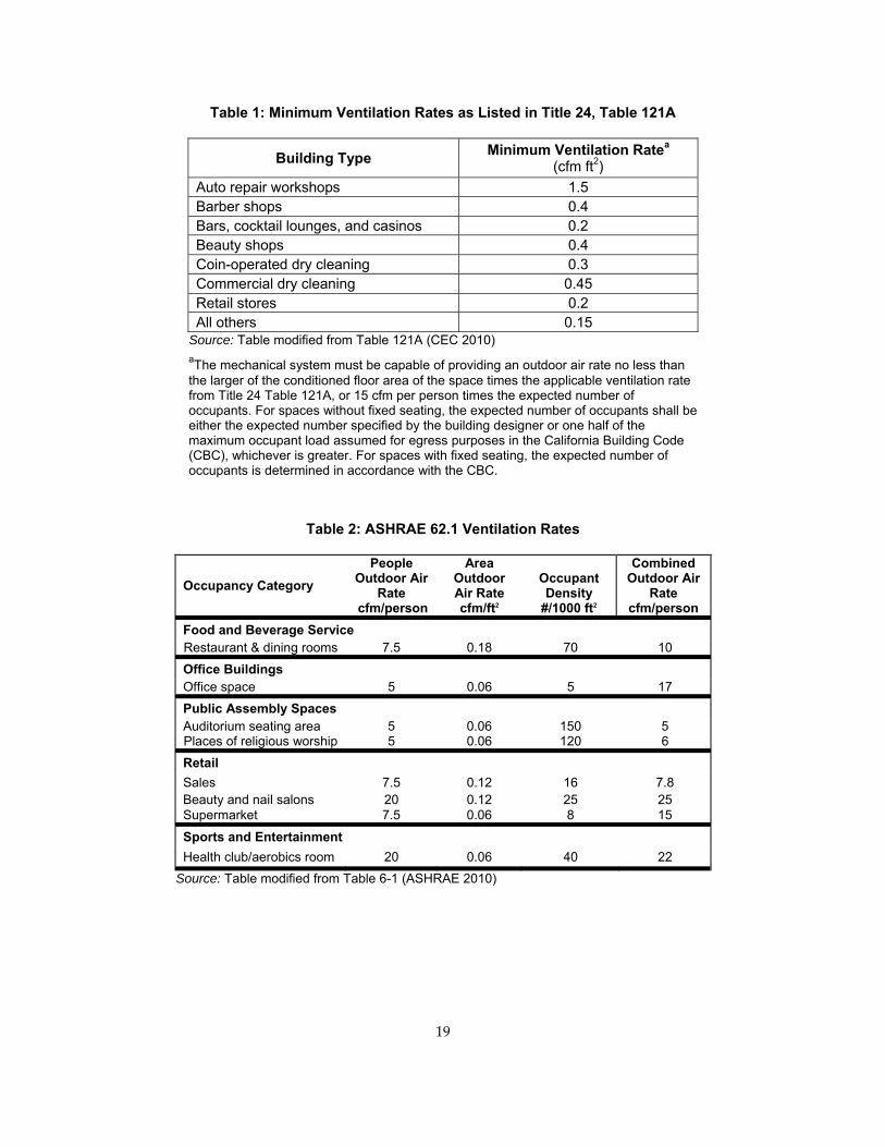
Table 1: Minimum Ventilation Rates as Listed in Title 24, Table 121A

Building Type Minimum Ventilation Ratea

(cfm ft2) Auto repair workshops 1.5 Barber shops 0.4 Bars, cocktail lounges, and casinos 0.2 Beauty shops 0.4 Coin-operated dry cleaning 0.3 Commercial dry cleaning 0.45 Retail stores 0.2 All others 0.15

Source: Table modified from Table 121A (CEC 2010) aThe mechanical system must be capable of providing an outdoor air rate no less than the larger of the conditioned floor area of the space times the applicable ventilation rate from Title 24 Table 121A, or 15 cfm per person times the expected number of occupants. For spaces without fixed seating, the expected number of occupants shall be either the expected number specified by the building designer or one half of the maximum occupant load assumed for egress purposes in the California Building Code (CBC), whichever is greater. For spaces with fixed seating, the expected number of occupants is determined in accordance with the CBC.

Table 2: ASHRAE 62.1 Ventilation Rates

Occupancy Category People

Outdoor Air Rate

cfm/person

Area Outdoor Air Rate cfm/ft2

Occupant Density

#/1000 ft2

Combined Outdoor Air

Rate cfm/person

Food and Beverage Service Restaurant & dining rooms 7.5 0.18 70 10

Office Buildings Office space 5 0.06 5 17

Public Assembly Spaces Auditorium seating area 5 0.06 150 5 Places of religious worship 5 0.06 120 6

Retail Sales 7.5 0.12 16 7.8 Beauty and nail salons 20 0.12 25 25 Supermarket 7.5 0.06 8 15

Sports and Entertainment Health club/aerobics room 20 0.06 40 22

Source: Table modified from Table 6-1 (ASHRAE 2010)  

 

19 

 

 

Carbon Dioxide Standards One relevant standard for CO2 is the Occupational Safety and Health Administration (OSHA) health standard, at a level of 5,000 ppmV (parts per million volume) (OSHA 1994).  A second relevant standard is Title 24, a standard set to define sufficient ventilation, which is 600 ppmV above the outdoor concentration, which is nominally defined as 400 ppmV if it is not measured (CEC 2008).  Title 24 implies that the comparison should be made at a steady‐state concentration, which theoretically is the building average maximum concentration.  This standard is similar to that set in ASHRAE 62.1, which is 700 ppmV (steady state is again implied) above the outdoor level, assuming outdoor levels typically vary between 300 and 500 ppmV (ASHRAE 2007). 

Temperature and Relative Humidity Standards The comfort levels described in ASHRAE Standard 55, as shown in Figure 1 (ASHRAE 2009) are also relevant for comparison.  The standard is defined in terms of operative temperature, which is the sum of the ambient temperature and a measure of the effectiveness of the incident radiant heating on occupants (ASHRAE 2009).  The summertime comfort standard is based on the clothing insulation value (Clo) assumption that people will be wearing a short‐sleeve shirt and cotton pants (0.5 Clo) while the wintertime standard is based on the assumption people will be wearing a business suit (1 Clo).  There are not clear time periods where the standard should be applied. 

20 

 

 

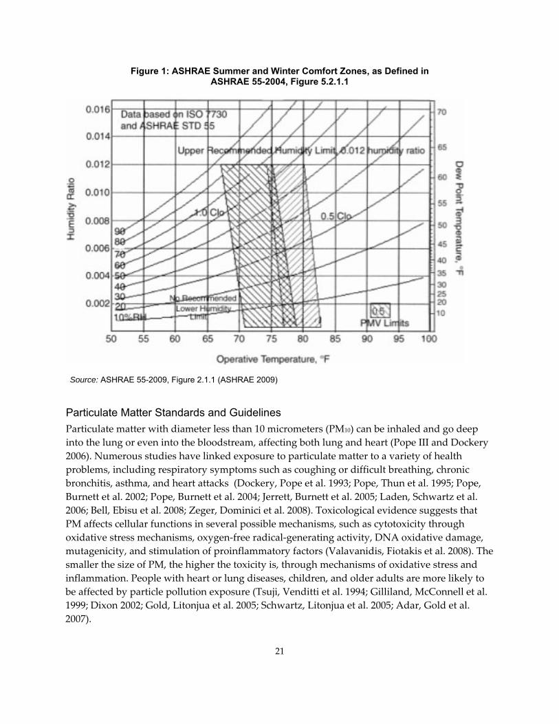
Figure 1: ASHRAE Summer and Winter Comfort Zones, as Defined in ASHRAE 55-2004, Figure 5.2.1.1

  Source: ASHRAE 55-2009, Figure 2.1.1 (ASHRAE 2009)

Particulate Matter Standards and Guidelines Particulate matter with diameter less than 10 micrometers (PM10) can be inhaled and go deep into the lung or even into the bloodstream, affecting both lung and heart (Pope III and Dockery 2006). Numerous studies have linked exposure to particulate matter to a variety of health problems, including respiratory symptoms such as coughing or difficult breathing, chronic bronchitis, asthma, and heart attacks  (Dockery, Pope et al. 1993; Pope, Thun et al. 1995; Pope, Burnett et al. 2002; Pope, Burnett et al. 2004; Jerrett, Burnett et al. 2005; Laden, Schwartz et al. 2006; Bell, Ebisu et al. 2008; Zeger, Dominici et al. 2008). Toxicological evidence suggests that PM affects cellular functions in several possible mechanisms, such as cytotoxicity through oxidative stress mechanisms, oxygen‐free radical‐generating activity, DNA oxidative damage, mutagenicity, and stimulation of proinflammatory factors (Valavanidis, Fiotakis et al. 2008). The smaller the size of PM, the higher the toxicity is, through mechanisms of oxidative stress and inflammation. People with heart or lung diseases, children, and older adults are more likely to be affected by particle pollution exposure (Tsuji, Venditti et al. 1994; Gilliland, McConnell et al. 1999; Dixon 2002; Gold, Litonjua et al. 2005; Schwartz, Litonjua et al. 2005; Adar, Gold et al. 2007). 

21 

 

 

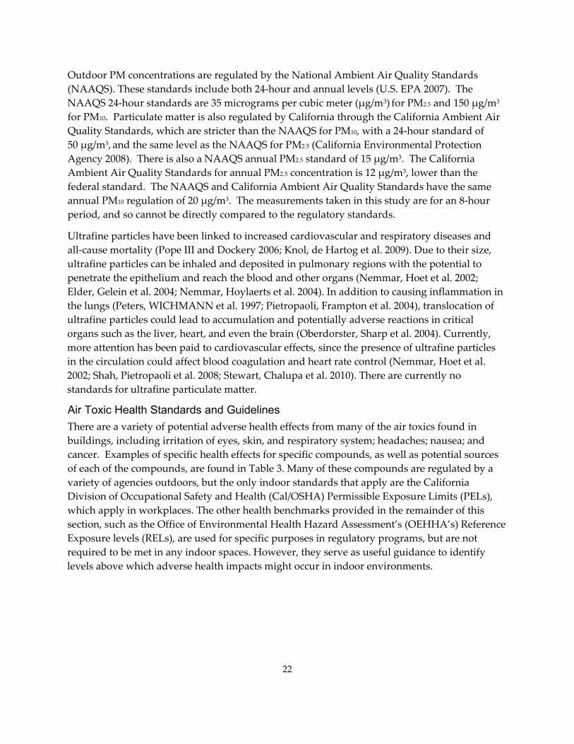
Outdoor PM concentrations are regulated by the National Ambient Air Quality Standards (NAAQS). These standards include both 24‐hour and annual levels (U.S. EPA 2007).  The NAAQS 24‐hour standards are 35 micrograms per cubic meter (μg/m3) for PM2.5 and 150 μg/m3 

for PM10.  Particulate matter is also regulated by California through the California Ambient Air Quality Standards, which are stricter than the NAAQS for PM10, with a 24‐hour standard of 50 μg/m3, and the same level as the NAAQS for PM2.5 (California Environmental Protection Agency 2008).  There is also a NAAQS annual PM2.5 standard of 15 μg/m3.  The California Ambient Air Quality Standards for annual PM2.5 concentration is 12 μg/m3, lower than the federal standard.  The NAAQS and California Ambient Air Quality Standards have the same annual PM10 regulation of 20 μg/m3.  The measurements taken in this study are for an 8‐hour period, and so cannot be directly compared to the regulatory standards. 

Ultrafine particles have been linked to increased cardiovascular and respiratory diseases and all‐cause mortality (Pope III and Dockery 2006; Knol, de Hartog et al. 2009). Due to their size, ultrafine particles can be inhaled and deposited in pulmonary regions with the potential to penetrate the epithelium and reach the blood and other organs (Nemmar, Hoet et al. 2002; Elder, Gelein et al. 2004; Nemmar, Hoylaerts et al. 2004). In addition to causing inflammation in the lungs (Peters, WICHMANN et al. 1997; Pietropaoli, Frampton et al. 2004), translocation of ultrafine particles could lead to accumulation and potentially adverse reactions in critical organs such as the liver, heart, and even the brain (Oberdorster, Sharp et al. 2004). Currently, more attention has been paid to cardiovascular effects, since the presence of ultrafine particles in the circulation could affect blood coagulation and heart rate control (Nemmar, Hoet et al. 2002; Shah, Pietropaoli et al. 2008; Stewart, Chalupa et al. 2010). There are currently no standards for ultrafine particulate matter. 

Air Toxic Health Standards and Guidelines There are a variety of potential adverse health effects from many of the air toxics found in buildings, including irritation of eyes, skin, and respiratory system; headaches; nausea; and cancer.  Examples of specific health effects for specific compounds, as well as potential sources of each of the compounds, are found in Table 3. Many of these compounds are regulated by a variety of agencies outdoors, but the only indoor standards that apply are the California  Division of Occupational Safety and Health (Cal/OSHA) Permissible Exposure Limits (PELs), which apply in workplaces. The other health benchmarks provided in the remainder of this section, such as the Office of Environmental Health Hazard Assessment’s (OEHHA’s) Reference Exposure levels (RELs), are used for specific purposes in regulatory programs, but are not required to be met in any indoor spaces. However, they serve as useful guidance to identify levels above which adverse health impacts might occur in indoor environments. 

22 

 

 

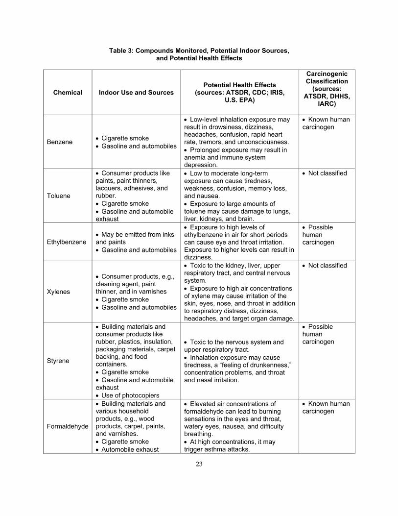
Table 3: Compounds Monitored, Potential Indoor Sources, and Potential Health Effects

Chemical Indoor Use and Sources Potential Health Effects

(sources: ATSDR, CDC; IRIS, U.S. EPA)

Carcinogenic Classification

(sources: ATSDR, DHHS,

IARC)

Benzene • Cigarette smoke • Gasoline and automobiles

• Low-level inhalation exposure may result in drowsiness, dizziness, headaches, confusion, rapid heart rate, tremors, and unconsciousness. • Prolonged exposure may result in anemia and immune system depression.

• Known human carcinogen

Toluene

• Consumer products like paints, paint thinners, lacquers, adhesives, and rubber. • Cigarette smoke • Gasoline and automobile exhaust

• Low to moderate long-term exposure can cause tiredness, weakness, confusion, memory loss, and nausea. • Exposure to large amounts of toluene may cause damage to lungs, liver, kidneys, and brain.

• Not classified

Ethylbenzene • May be emitted from inks and paints • Gasoline and automobiles

• Exposure to high levels of ethylbenzene in air for short periods can cause eye and throat irritation. Exposure to higher levels can result in dizziness.

• Possible human carcinogen

Xylenes

• Consumer products, e.g., cleaning agent, paint thinner, and in varnishes • Cigarette smoke • Gasoline and automobiles

• Toxic to the kidney, liver, upper respiratory tract, and central nervous system. • Exposure to high air concentrations of xylene may cause irritation of the skin, eyes, nose, and throat in addition to respiratory distress, dizziness, headaches, and target organ damage.

• Not classified

Styrene

• Building materials and consumer products like rubber, plastics, insulation, packaging materials, carpet backing, and food containers. • Cigarette smoke • Gasoline and automobile exhaust • Use of photocopiers

• Toxic to the nervous system and upper respiratory tract. • Inhalation exposure may cause tiredness, a “feeling of drunkenness,” concentration problems, and throat and nasal irritation.

• Possible human carcinogen

Formaldehyde

• Building materials and various household products, e.g., wood products, carpet, paints, and varnishes. • Cigarette smoke • Automobile exhaust

• Elevated air concentrations of formaldehyde can lead to burning sensations in the eyes and throat, watery eyes, nausea, and difficulty breathing. • At high concentrations, it may trigger asthma attacks.

• Known human carcinogen

23 

 

 

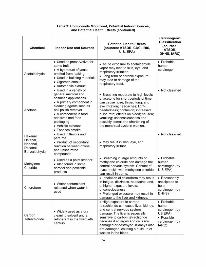
Table 3: Compounds Monitored, Potential Indoor Sources, and Potential Health Effects (continued)

Chemical Indoor Use and Sources Potential Health Effects

(sources: ATSDR, CDC; IRIS, U.S. EPA)

Carcinogenic Classification

(sources: ATSDR,

DHHS, IARC)

Acetaldehyde

• Used as preservative for some fruit • A byproduct of yeast emitted from baking • Used in building materials • Cigarette smoke • Automobile exhaust

• Acute exposure to acetaldehyde vapor may lead to skin, eye, and respiratory irritation. • Long-term or chronic exposure may lead to damage of the respiratory tract.

• Probable human carcinogen

Acetone

• Used in a variety of general medical and cosmetic applications • A primary component in cleaning agents such as nail polish remover • A component in food additives and food packaging • Vehicle exhaust • Tobacco smoke

• Breathing moderate to high levels of acetone for short periods of time can cause nose, throat, lung, and eye irritation; headaches; light-headedness; confusion; increased pulse rate; effects on blood; nausea; vomiting; unconsciousness and possibly coma; and shortening of the menstrual cycle in women.

• Not classified

Hexanal, Octanal, Nonanal, Decanal, Benzaldehyde

• Used in flavors and perfume • Product of secondary reaction between ozone and unsaturated compounds

• May result in skin, eye, and respiratory irritant

• Not classified

Methylene Chloride

• Used as a paint stripper • Also found in some aerosol and pesticide products

• Breathing in large amounts of methylene chloride can damage the central nervous system. Contact of eyes or skin with methylene chloride can result in burns.

• Probable human carcinogen (by U.S EPA)

Chloroform • Water contaminant released when water is used

• Inhalation of chloroform may result in fatigue, dizziness, headache, and, at higher exposure levels, unconsciousness. • Prolonged exposure may result in damage to the liver and kidneys.

• Reasonably anticipated to be a carcinogen (by DHHS)

Carbon Tetrachloride

• Widely used as a dry cleaning solvent and a refrigerant in the twentieth century

• High exposure to carbon tetrachloride can cause liver, kidney, and central nervous system damage. The liver is especially sensitive to carbon tetrachloride because it enlarges and cells are damaged or destroyed. Kidneys also are damaged, causing a build up of wastes in the blood.

• Probable human carcinogen (by US EPA) • Possible carcinogen (by IARC)

24 

 

 

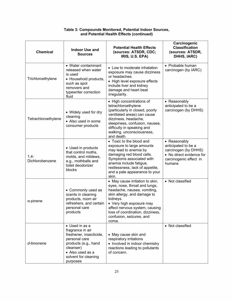
25 

 

Table 3: Compounds Monitored, Potential Indoor Sources, and Potential Health Effects (continued)

Chemical Indoor Use and Sources

Potential Health Effects (sources: ATSDR, CDC;

IRIS, U.S. EPA)

Carcinogenic Classification

(sources: ATSDR, DHHS, IARC)

Trichloroethylene

• Water contaminant released when water is used • Household products, such as spot removers and typewriter correction fluid

• Low to moderate inhalation exposure may cause dizziness or headaches. • High level exposure effects include liver and kidney damage and heart beat irregularity.

• Probable human carcinogen (by IARC)

Tetrachloroethylene

• Widely used for dry cleaning • Also used in some consumer products

• High concentrations of tetrachloroethylene (particularly in closed, poorly ventilated areas) can cause dizziness, headache, sleepiness, confusion, nausea, difficulty in speaking and walking, unconsciousness, and death.

• Reasonably anticipated to be a carcinogen (by DHHS)

1,4-Dichlorobenzene

• Used in products that control moths, molds, and mildews, e.g., mothballs and toilet deodorizer blocks

• Toxic to the blood and exposure to large amounts may lead to anemia by damaging red blood cells. Symptoms associated with anemia include fatigue, restlessness, lack of appetite, and a pale appearance to your skin.

• Reasonably anticipated to be a carcinogen (by DHHS) • No direct evidence for carcinogenic effect in humans

α-pinene

• Commonly used as scents in cleaning products, room air refreshers, and certain personal care products

• May cause irritation to skin, eyes, nose, throat and lungs, headache, nausea, vomiting, skin allergy, and damage to kidneys. • Very high exposure may affect nervous system, causing loss of coordination, dizziness, confusion, seizures, and coma.

• Not classified

d-limonene

• Used in as a fragrance in air freshener, insecticide, personal care products (e.g., hand cleanser) • Also used as a solvent for cleaning purposes

• May cause skin and respiratory irritations • Involved in indoor chemistry reactions leading to pollutants of concern.

• Not classified

 

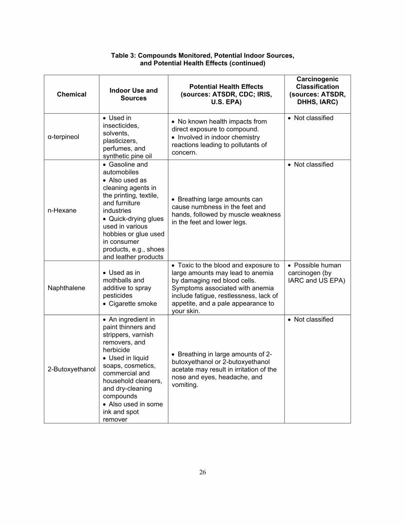
Table 3: Compounds Monitored, Potential Indoor Sources, and Potential Health Effects (continued)

Chemical Indoor Use and Sources

Potential Health Effects (sources: ATSDR, CDC; IRIS,

U.S. EPA)

Carcinogenic Classification

(sources: ATSDR, DHHS, IARC)

α-terpineol

• Used in insecticides, solvents, plasticizers, perfumes, and synthetic pine oil

• No known health impacts from direct exposure to compound. • Involved in indoor chemistry reactions leading to pollutants of concern.

• Not classified

n-Hexane

• Gasoline and automobiles • Also used as cleaning agents in the printing, textile, and furniture industries • Quick-drying glues used in various hobbies or glue used in consumer products, e.g., shoes and leather products

• Breathing large amounts can cause numbness in the feet and hands, followed by muscle weakness in the feet and lower legs.

• Not classified

Naphthalene

• Used as in mothballs and additive to spray pesticides • Cigarette smoke

• Toxic to the blood and exposure to large amounts may lead to anemia by damaging red blood cells. Symptoms associated with anemia include fatigue, restlessness, lack of appetite, and a pale appearance to your skin.

• Possible human carcinogen (by IARC and US EPA)

2-Butoxyethanol

• An ingredient in paint thinners and strippers, varnish removers, and herbicide • Used in liquid soaps, cosmetics, commercial and household cleaners, and dry-cleaning compounds • Also used in some ink and spot remover

• Breathing in large amounts of 2-butoxyethanol or 2-butoxyethanol acetate may result in irritation of the nose and eyes, headache, and vomiting.

• Not classified

26 

 

 

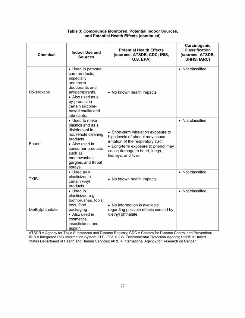
Table 3: Compounds Monitored, Potential Indoor Sources, and Potential Health Effects (continued)

Chemical Indoor Use and Sources

Potential Health Effects (sources: ATSDR, CDC; IRIS,

U.S. EPA)

Carcinogenic Classification

(sources: ATSDR, DHHS, IARC)

D5-siloxane

• Used in personal care products, especially underarm deodorants and antiperspirants. • Also used as a by-product in certain silicone-based caulks and lubricants.

• No known health impacts

• Not classified

Phenol

• Used to make plastics and as a disinfectant in household cleaning products • Also used in consumer products such as mouthwashes, gargles, and throat sprays

• Short-term inhalation exposure to high levels of phenol may cause irritation of the respiratory tract. • Long-term exposure to phenol may cause damage to heart, lungs, kidneys, and liver.

• Not classified

TXIB

• Used as a plasticizer in certain vinyl products

• No known health impacts

• Not classified

Diethylphthalate

• Used in plasticizer, e.g., toothbrushes, tools, toys, food packaging • Also used in cosmetics, insecticides, and aspirin

• No information is available regarding possible effects caused by diethyl phthalate.

• Not classified

ATSDR = Agency for Toxic Substances and Disease Registry; CDC = Centers for Disease Control and Prevention; IRIS = Integrated Risk Information System; U.S. EPA = U.S. Environmental Protection Agency; DHHS = United States Department of Health and Human Services; IARC = International Agency for Research on Cancer

27 

 

 

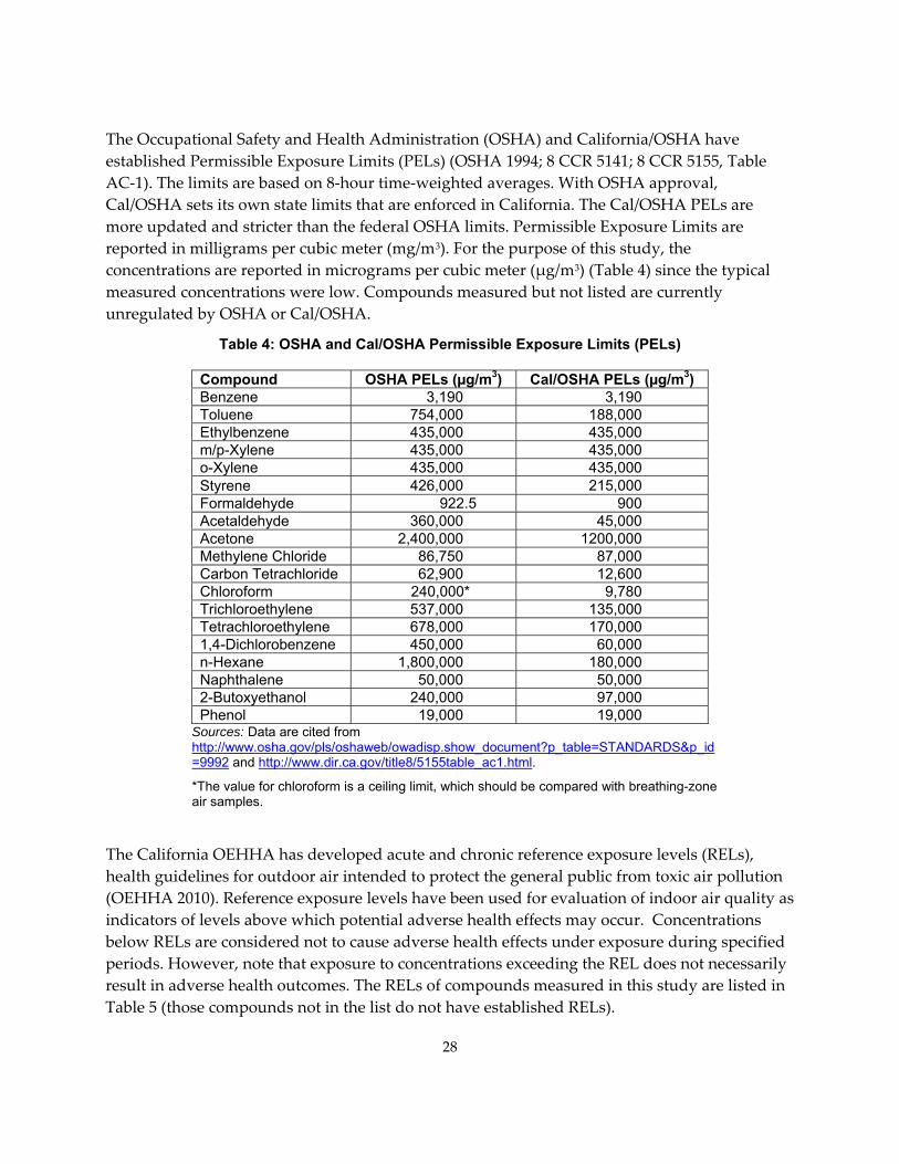
 The Occupational Safety and Health Administration (OSHA) and California/OSHA have established Permissible Exposure Limits (PELs) (OSHA 1994; 8 CCR 5141; 8 CCR 5155, Table AC‐1). The limits are based on 8‐hour time‐weighted averages. With OSHA approval, Cal/OSHA sets its own state limits that are enforced in California. The Cal/OSHA PELs are more updated and stricter than the federal OSHA limits. Permissible Exposure Limits are reported in milligrams per cubic meter (mg/m3). For the purpose of this study, the concentrations are reported in micrograms per cubic meter (μg/m3) (Table 4) since the typical measured concentrations were low. Compounds measured but not listed are currently unregulated by OSHA or Cal/OSHA.  

Table 4: OSHA and Cal/OSHA Permissible Exposure Limits (PELs)

Compound OSHA PELs (µg/m3) Cal/OSHA PELs (µg/m3) Benzene 3,190 3,190 Toluene 754,000 188,000 Ethylbenzene 435,000 435,000 m/p-Xylene 435,000 435,000 o-Xylene 435,000 435,000 Styrene 426,000 215,000 Formaldehyde 922.5 900 Acetaldehyde 360,000 45,000 Acetone 2,400,000 1200,000 Methylene Chloride 86,750 87,000 Carbon Tetrachloride 62,900 12,600 Chloroform 240,000* 9,780 Trichloroethylene 537,000 135,000 Tetrachloroethylene 678,000 170,000 1,4-Dichlorobenzene 450,000 60,000 n-Hexane 1,800,000 180,000 Naphthalene 50,000 50,000 2-Butoxyethanol 240,000 97,000 Phenol 19,000 19,000

Sources: Data are cited from http://www.osha.gov/pls/oshaweb/owadisp.show_document?p_table=STANDARDS&p_id=9992 and http://www.dir.ca.gov/title8/5155table_ac1.html.

*The value for chloroform is a ceiling limit, which should be compared with breathing-zone air samples. 

   The California OEHHA has developed acute and chronic reference exposure levels (RELs), health guidelines for outdoor air intended to protect the general public from toxic air pollution  (OEHHA 2010). Reference exposure levels have been used for evaluation of indoor air quality as indicators of levels above which potential adverse health effects may occur.  Concentrations below RELs are considered not to cause adverse health effects under exposure during specified periods. However, note that exposure to concentrations exceeding the REL does not necessarily result in adverse health outcomes. The RELs of compounds measured in this study are listed in Table 5 (those compounds not in the list do not have established RELs). 

28 

 

 

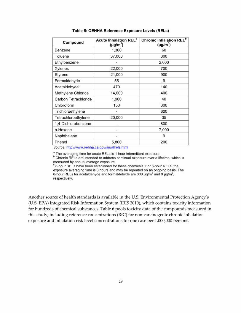
Table 5: OEHHA Reference Exposure Levels (RELs) 

Compound Acute Inhalation RELa (µg/m3)

Chronic Inhalation RELb (µg/m3)

Benzene 1,300 60 Toluene 37,000 300 Ethylbenzene - 2,000 Xylenes 22,000 700 Styrene 21,000 900 Formaldehydec 55 9 Acetaldehydec 470 140 Methylene Chloride 14,000 400 Carbon Tetrachloride 1,900 40 Chloroform 150 300 Trichloroethylene - 600 Tetrachloroethylene 20,000 35 1,4-Dichlorobenzene - 800 n-Hexane - 7,000 Naphthalene - 9 Phenol 5,800 200

Source: http://www.oehha.ca.gov/air/allrels.html a The averaging time for acute RELs is 1-hour intermittent exposure. b Chronic RELs are intended to address continual exposure over a lifetime, which is measured by annual average exposure. c 8-hour RELs have been established for these chemicals. For 8-hour RELs, the exposure averaging time is 8 hours and may be repeated on an ongoing basis. The 8-hour RELs for acetaldehyde and formaldehyde are 300 µg/m3 and 9 µg/m3, respectively.

 

Another source of health standards is available in the U.S. Environmental Protection Agency’s (U.S. EPA) Integrated Risk Information System (IRIS 2010), which contains toxicity information for hundreds of chemical substances. Table 6 pools toxicity data of the compounds measured in this study, including reference concentrations (RfC) for non‐carcinogenic chronic inhalation exposure and inhalation risk level concentrations for one case per 1,000,000 persons.  

29 

 

 

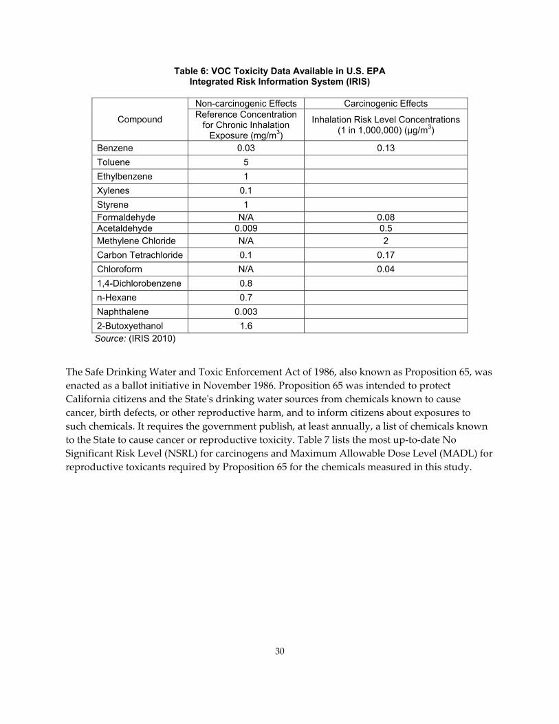
Table 6: VOC Toxicity Data Available in U.S. EPA Integrated Risk Information System (IRIS) 

Compound

Non-carcinogenic Effects Carcinogenic Effects Reference Concentration

for Chronic Inhalation Exposure (mg/m3)

Inhalation Risk Level Concentrations (1 in 1,000,000) (µg/m3)

Benzene 0.03 0.13 Toluene 5 Ethylbenzene 1 Xylenes 0.1 Styrene 1 Formaldehyde N/A 0.08 Acetaldehyde 0.009 0.5 Methylene Chloride N/A 2 Carbon Tetrachloride 0.1 0.17 Chloroform N/A 0.04 1,4-Dichlorobenzene 0.8 n-Hexane 0.7 Naphthalene 0.003 2-Butoxyethanol 1.6 Source: (IRIS 2010)

 

The Safe Drinking Water and Toxic Enforcement Act of 1986, also known as Proposition 65, was enacted as a ballot initiative in November 1986. Proposition 65 was intended to protect California citizens and the Stateʹs drinking water sources from chemicals known to cause cancer, birth defects, or other reproductive harm, and to inform citizens about exposures to such chemicals. It requires the government publish, at least annually, a list of chemicals known to the State to cause cancer or reproductive toxicity. Table 7 lists the most up‐to‐date No Significant Risk Level (NSRL) for carcinogens and Maximum Allowable Dose Level (MADL) for reproductive toxicants required by Proposition 65 for the chemicals measured in this study. 

 

 

 

 

 

30 

 

 

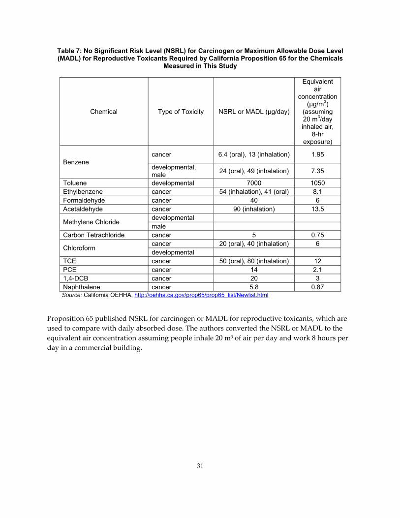
Table 7: No Significant Risk Level (NSRL) for Carcinogen or Maximum Allowable Dose Level (MADL) for Reproductive Toxicants Required by California Proposition 65 for the Chemicals

Measured in This Study

Chemical Type of Toxicity NSRL or MADL (µg/day)

Equivalent air

concentration (µg/m3)

(assuming 20 m3/day inhaled air,

8-hr exposure)

Benzene cancer 6.4 (oral), 13 (inhalation) 1.95

developmental, male 24 (oral), 49 (inhalation) 7.35

Toluene developmental 7000 1050 Ethylbenzene cancer 54 (inhalation), 41 (oral) 8.1 Formaldehyde cancer 40 6 Acetaldehyde cancer 90 (inhalation) 13.5

Methylene Chloride developmental male

Carbon Tetrachloride cancer 5 0.75

Chloroform cancer 20 (oral), 40 (inhalation) 6 developmental

TCE cancer 50 (oral), 80 (inhalation) 12 PCE cancer 14 2.1 1,4-DCB cancer 20 3 Naphthalene cancer 5.8 0.87 Source: California OEHHA, http://oehha.ca.gov/prop65/prop65_list/Newlist.html

 

Proposition 65 published NSRL for carcinogen or MADL for reproductive toxicants, which are used to compare with daily absorbed dose. The authors converted the NSRL or MADL to the equivalent air concentration assuming people inhale 20 m3 of air per day and work 8 hours per day in a commercial building. 

31 

 

 

CHAPTER 2: Methods Building Selection This project’s goal was to include 37 unique buildings, sampling 3 of them at two points in time, to reach a total of 40 days of sampling.  To sample a wide range of buildings, the authors considered multiple attributes when recruiting the buildings, specifically distributed by region, size, and building use.  The buildings were primarily selected from those contacted in the SMCB phone survey (Piazza and Apte 2010), with the remainder being selected as either a convenience sample or in a semi‐random manner. 

Distribution of Buildings in California As the desire was to sample a representative distribution of buildings in the State in terms of size and function, the researchers needed to determine that distribution.  The initial plan for defining the size and building use for the study population was to use the results of the SMCB phone survey. However, because it appeared that data collection delays in the SMCB phone survey would cause considerable delays in this project, alternative approaches were used.   

The distribution of buildings by type was also needed.  Building types are often defined as follows: 

• Offices: non‐medical – Includes traditional office buildings along with banking and other financial service buildings, laboratories, and research and development facilities 

• Restaurant food service – Includes sit‐down, counter order, cafeteria, and coffee shop facilities 

• Food Stores – Includes grocery stores, liquor stores, and convenience stores without gasoline 

• Retail – All retail facilities 

• Healthcare – Includes hospitals, urgent care, doctor’s offices, medical laboratories, and other types (dental, chiropractor) of medial service buildings, as well as nursing homes 

• Lodging – All lodging facilities 

• Public Assembly – Includes health/fitness centers, churches, movie theaters, museums, libraries, and other assembly facilities 

• Services – Includes beauty salons, auto repair/gas (including gas station convenience stores), other repair shops 

• Miscellaneous ‐ Includes post offices, police and fire stations, and light manufacturing 

 

One study containing information on uses of California buildings is The California Commercial End Use Survey (CEUS), conducted by Itron, Inc., under contract to the California Energy Commission (Itron Inc. 2006).  The survey consists of a detailed inventory of building 

32 

 

 

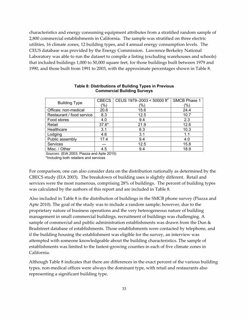
characteristics and energy consuming equipment attributes from a stratified random sample of 2,800 commercial establishments in California.  The sample was stratified on three electric utilities, 16 climate zones, 12 building types, and 4 annual energy consumption levels.  The CEUS database was provided by the Energy Commission.  Lawrence Berkeley National Laboratory was able to run the dataset to compile a listing (excluding warehouses and schools) that included buildings 1,000 to 50,000 square feet, for those buildings built between 1979 and 1990, and those built from 1991 to 2003, with the approximate percentages shown in Table 8. 

 

Table 8: Distributions of Building Types in Previous Commercial Building Surveys

Building Type CBECS(%)

CEUS 1979–2003 < 50000 ft2(%)

SMCB Phase 1(%)

Offices: non-medical 20.6 15.6 24.4 Restaurant / food service 8.3 12.5 10.7 Food stores 4.0 9.4 2.3 Retail 37.6* 21.9 12.6 Healthcare 3.1 6.3 10.3 Lodging 4.6 3.1 1.1 Public assembly 17.4 9.4 4.0 Services — 12.5 15.8 Misc. / Other 4.5 9.4 18.9

Sources: (EIA 2003; Piazza and Apte 2010) *Including both retailers and services

For comparison, one can also consider data on the distribution nationally as determined by the CBECS study (EIA 2003).  The breakdown of building uses is slightly different.  Retail and services were the most numerous, comprising 28% of buildings.  The percent of building types was calculated by the authors of this report and are included in Table 8. 

Also included in Table 8 is the distribution of buildings in the SMCB phone survey (Piazza and Apte 2010). The goal of the study was to include a random sample; however, due to the proprietary nature of business operations and the very heterogeneous nature of building management in small commercial buildings, recruitment of buildings was challenging. A sample of commercial and public administration establishments was drawn from the Dun & Bradstreet database of establishments. Those establishments were contacted by telephone, and if the building housing the establishment was eligible for the survey, an interview was attempted with someone knowledgeable about the building characteristics. The sample of establishments was limited to the fastest‐growing counties in each of five climate zones in California. 

Although Table 8 indicates that there are differences in the exact percent of the various building types, non‐medical offices were always the dominant type, with retail and restaurants also representing a significant building type. 

33 

 

 

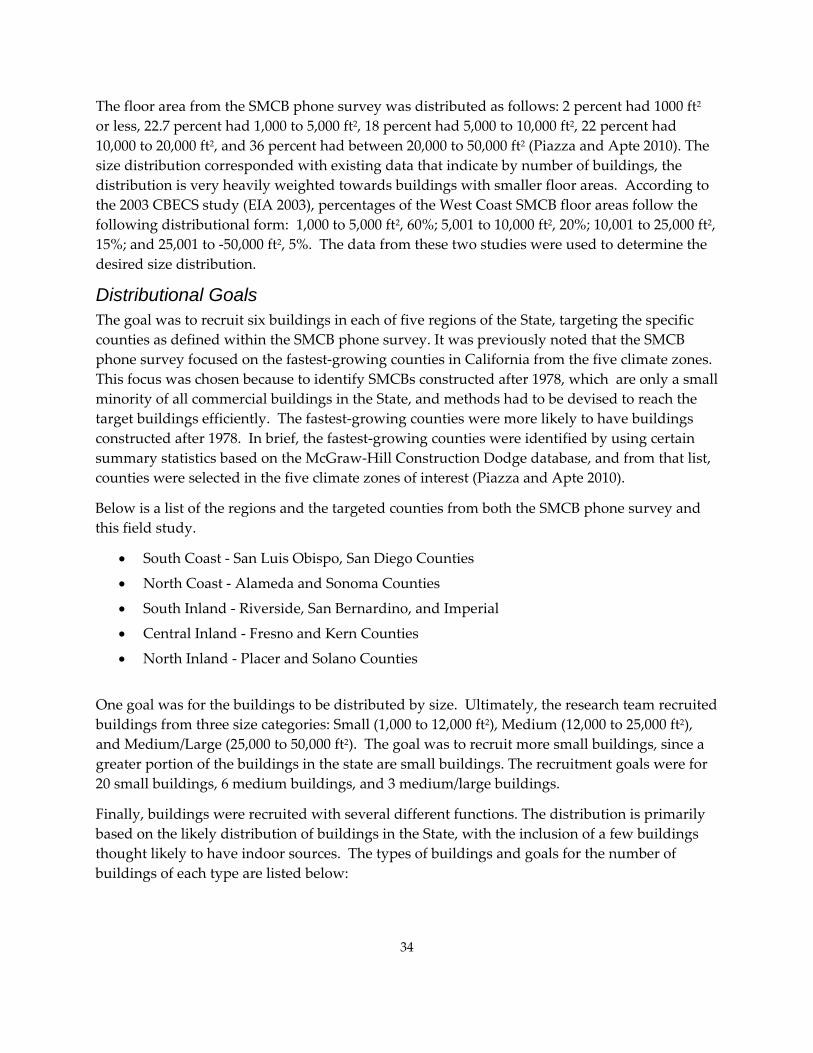
The floor area from the SMCB phone survey was distributed as follows: 2 percent had 1000 ft2 or less, 22.7 percent had 1,000 to 5,000 ft2, 18 percent had 5,000 to 10,000 ft2, 22 percent had 10,000 to 20,000 ft2, and 36 percent had between 20,000 to 50,000 ft2 (Piazza and Apte 2010). The size distribution corresponded with existing data that indicate by number of buildings, the distribution is very heavily weighted towards buildings with smaller floor areas.  According to the 2003 CBECS study (EIA 2003), percentages of the West Coast SMCB floor areas follow the following distributional form:  1,000 to 5,000 ft2, 60%; 5,001 to 10,000 ft2, 20%; 10,001 to 25,000 ft2, 15%; and 25,001 to ‐50,000 ft2, 5%.  The data from these two studies were used to determine the desired size distribution.   

Distributional Goals The goal was to recruit six buildings in each of five regions of the State, targeting the specific counties as defined within the SMCB phone survey. It was previously noted that the SMCB phone survey focused on the fastest‐growing counties in California from the five climate zones.  This focus was chosen because to identify SMCBs constructed after 1978, which  are only a small minority of all commercial buildings in the State, and methods had to be devised to reach the target buildings efficiently.  The fastest‐growing counties were more likely to have buildings constructed after 1978.  In brief, the fastest‐growing counties were identified by using certain summary statistics based on the McGraw‐Hill Construction Dodge database, and from that list, counties were selected in the five climate zones of interest (Piazza and Apte 2010). 

Below is a list of the regions and the targeted counties from both the SMCB phone survey and this field study. 

• South Coast ‐ San Luis Obispo, San Diego Counties  

• North Coast ‐ Alameda and Sonoma Counties   

• South Inland ‐ Riverside, San Bernardino, and Imperial   

• Central Inland ‐ Fresno and Kern Counties   

• North Inland ‐ Placer and Solano Counties    One goal was for the buildings to be distributed by size.  Ultimately, the research team recruited buildings from three size categories: Small (1,000 to 12,000 ft2), Medium (12,000 to 25,000 ft2), and Medium/Large (25,000 to 50,000 ft2).  The goal was to recruit more small buildings, since a greater portion of the buildings in the state are small buildings. The recruitment goals were for 20 small buildings, 6 medium buildings, and 3 medium/large buildings. 

Finally, buildings were recruited with several different functions. The distribution is primarily based on the likely distribution of buildings in the State, with the inclusion of a few buildings thought likely to have indoor sources.  The types of buildings and goals for the number of buildings of each type are listed below: 

34 

 

 

 • Restaurants: 4 buildings  

• Retail: 6 buildings  

• Office: 7 buildings  

• Gym: 2 buildings  

• Gas Station: 2 buildings  

• Beauty Salons: 2 buildings  

• Dental Offices: 2 buildings   

• Healthcare: 2 buildings  

• Grocery Store: 2 buildings  

• Religious/Public Assembly: 2 buildings   

• Other: There were no goals for this category 

Building Selection Procedures Three methods were used to select buildings for the study. The first method involved a two‐step process linked to the SMCB phone survey (Piazza and Apte 2010).  In that survey, a sample of commercial and public administration establishments was drawn from the Dun & Bradstreet (www.dnb.com) database of establishments.  The research team surveyed 476 establishments (buildings) in the SMCB phone survey (a 35.6 percent response rate), collecting information on the physical and operational characteristics of their facilities.  At the end of each survey, the research team asked the person completing the interview if they would be interested in participating in a follow‐up field study.  Overall, 73 percent of the establishments indicated that they were interested in learning more about the field study.  The distribution of the interested building participants is categorized by region in Table 9. 

Table 9: Number of Buildings Interested in Learning More About the Field Survey

Central Inland

North Coast

North Inland

South Coast

South Inland

Total Percent

No 30 20 29 20 30 129 27 Yes 80 60 72 63 72 347 73 Total 110 80 101 83 102 476  

The second recruitment method included buildings brought into the study as a convenience sample.  The third recruitment method used selection of buildings from a publicly available phone listing, generally Google™ listings of specific types of establishments in a region.   

 35 

 

 

36 

 

Heating, Ventilation, and Air-Conditioning Systems The following sections describe methods used to collect information about the HVAC system obtained through a building inspection, measurements of air exchange, and carbon dioxide concentrations. It was anticipated that buildings would primarily have rooftop package HVAC units and methods for evaluation are based on this assumption. Due to the largely disaggregated, heterogeneous nature of commercial enterprise, information on SMCB operation and maintenance (O&M) is very limited.  Research on large commercial buildings has shown that O&M is variable, and IEQ suffers due to poor maintenance. It is anticipated that information on SMCBs will reflect similar or greater variability. Methods for measurement of temperature and relative humidity are also specified.   

Characterization of Physical Plant: Maintenance and Operation of Building, Focus on HVAC and Air Filtration Systems The research team inspected air handling units on site to determine condition.  If there were three or less units, all units were inspected.  If there were more than three units, three units were selected to be inspected.  If there were multiple units of the same model, one of that type of unit was generally inspected.  The research team also gave preference to units thought likely to have a larger air intake.  The inspection log was primarily based on the log developed for the BASE study.  A list of the criteria inspected is shown in Table 10 below. 

In addition, the research team determined how frequently the units were inspected and the reasons inspections were conducted.  The questions related to maintenance can be found in Appendix A, Table A.20.  

 

 

 

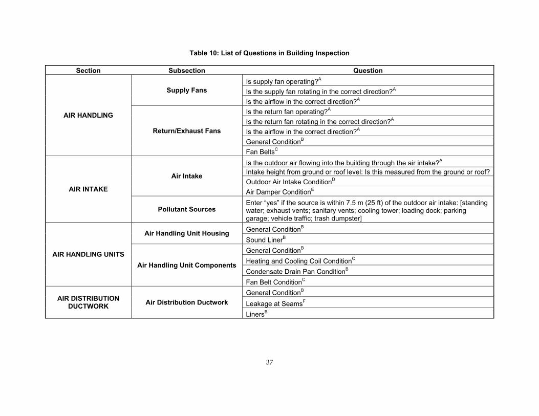
Table 10: List of Questions in Building Inspection

Section Subsection Question

AIR HANDLING

Supply Fans Is supply fan operating?A Is the supply fan rotating in the correct direction?A Is the airflow in the correct direction?A

Return/Exhaust Fans

Is the return fan operating?A Is the return fan rotating in the correct direction?A Is the airflow in the correct direction?A General ConditionB Fan BeltsC

AIR INTAKE

Air Intake

Is the outdoor air flowing into the building through the air intake?A Intake height from ground or roof level: Is this measured from the ground or roof? Outdoor Air Intake ConditionD Air Damper ConditionE

Pollutant Sources Enter “yes” if the source is within 7.5 m (25 ft) of the outdoor air intake: [standing water; exhaust vents; sanitary vents; cooling tower; loading dock; parking garage; vehicle traffic; trash dumpster]

AIR HANDLING UNITS

Air Handling Unit Housing General ConditionB Sound LinerB

Air Handling Unit Components

General ConditionB Heating and Cooling Coil ConditionC Condensate Drain Pan ConditionB Fan Belt ConditionC

AIR DISTRIBUTION DUCTWORK Air Distribution Ductwork

General ConditionB Leakage at SeamsF LinersB

 

 

37 

 

 

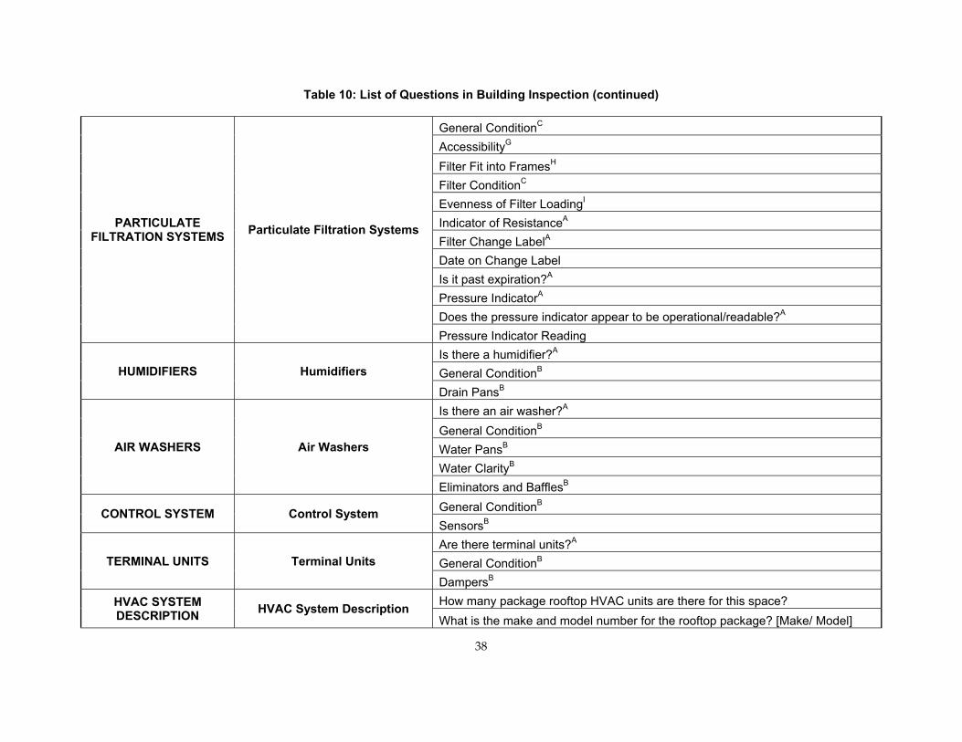
Table 10: List of Questions in Building Inspection (continued)

PARTICULATE FILTRATION SYSTEMS Particulate Filtration Systems

General ConditionC AccessibilityG Filter Fit into FramesH Filter ConditionC Evenness of Filter LoadingI Indicator of ResistanceA Filter Change LabelA Date on Change Label Is it past expiration?A Pressure IndicatorA Does the pressure indicator appear to be operational/readable?A Pressure Indicator Reading

HUMIDIFIERS Humidifiers Is there a humidifier?A General ConditionB Drain PansB

AIR WASHERS Air Washers

Is there an air washer?A General ConditionB Water PansB Water ClarityB Eliminators and BafflesB

CONTROL SYSTEM Control System General ConditionB SensorsB

TERMINAL UNITS Terminal Units Are there terminal units?A General ConditionB DampersB

HVAC SYSTEM DESCRIPTION HVAC System Description How many package rooftop HVAC units are there for this space?

What is the make and model number for the rooftop package? [Make/ Model]

38 

 

 

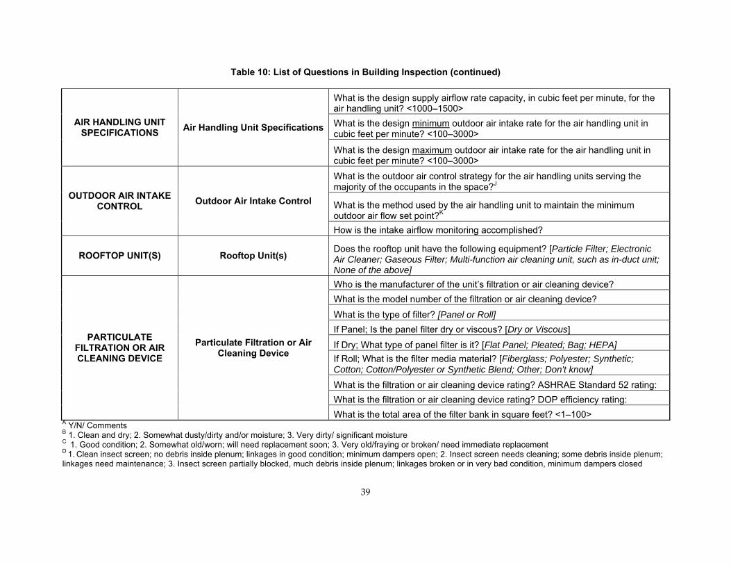
Table 10: List of Questions in Building Inspection (continued)

AIR HANDLING UNIT SPECIFICATIONS Air Handling Unit Specifications

What is the design supply airflow rate capacity, in cubic feet per minute, for the air handling unit? <1000–1500> What is the design minimum outdoor air intake rate for the air handling unit in cubic feet per minute? <100–3000>

What is the design maximum outdoor air intake rate for the air handling unit in cubic feet per minute? <100–3000>

OUTDOOR AIR INTAKE CONTROL Outdoor Air Intake Control

What is the outdoor air control strategy for the air handling units serving the majority of the occupants in the space?J

What is the method used by the air handling unit to maintain the minimum outdoor air flow set point?K How is the intake airflow monitoring accomplished?

ROOFTOP UNIT(S) Rooftop Unit(s) Does the rooftop unit have the following equipment? [Particle Filter; Electronic Air Cleaner; Gaseous Filter; Multi-function air cleaning unit, such as in-duct unit; None of the above]

PARTICULATE FILTRATION OR AIR CLEANING DEVICE

Particulate Filtration or Air Cleaning Device

Who is the manufacturer of the unit’s filtration or air cleaning device? What is the model number of the filtration or air cleaning device?

What is the type of filter? [Panel or Roll] If Panel; Is the panel filter dry or viscous? [Dry or Viscous]

If Dry; What type of panel filter is it? [Flat Panel; Pleated; Bag; HEPA] If Roll; What is the filter media material? [Fiberglass; Polyester; Synthetic; Cotton; Cotton/Polyester or Synthetic Blend; Other; Don't know]

What is the filtration or air cleaning device rating? ASHRAE Standard 52 rating: What is the filtration or air cleaning device rating? DOP efficiency rating: What is the total area of the filter bank in square feet? <1–100>

A Y/N/ Comments B 1. Clean and dry; 2. Somewhat dusty/dirty and/or moisture; 3. Very dirty/ significant moisture C 1. Good condition; 2. Somewhat old/worn; will need replacement soon; 3. Very old/fraying or broken/ need immediate replacement D 1. Clean insect screen; no debris inside plenum; linkages in good condition; minimum dampers open; 2. Insect screen needs cleaning; some debris inside plenum; linkages need maintenance; 3. Insect screen partially blocked, much debris inside plenum; linkages broken or in very bad condition, minimum dampers closed

39 

 

 

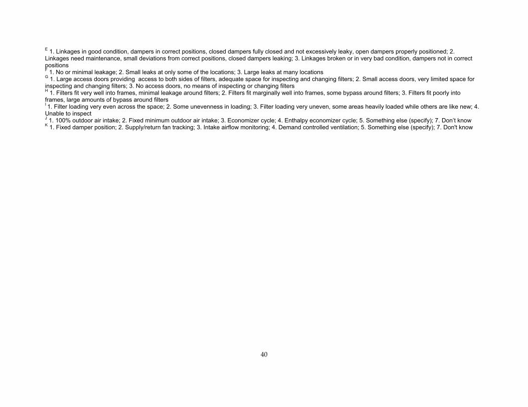
40 

 

E 1. Linkages in good condition, dampers in correct positions, closed dampers fully closed and not excessively leaky, open dampers properly positioned; 2. Linkages need maintenance, small deviations from correct positions, closed dampers leaking; 3. Linkages broken or in very bad condition, dampers not in correct positions F 1. No or minimal leakage; 2. Small leaks at only some of the locations; 3. Large leaks at many locations G 1. Large access doors providing access to both sides of filters, adequate space for inspecting and changing filters; 2. Small access doors, very limited space for inspecting and changing filters; 3. No access doors, no means of inspecting or changing filters H 1. Filters fit very well into frames, minimal leakage around filters; 2. Filters fit marginally well into frames, some bypass around filters; 3. Filters fit poorly into frames, large amounts of bypass around filters

I 1. Filter loading very even across the space; 2. Some unevenness in loading; 3. Filter loading very uneven, some areas heavily loaded while others are like new; 4. Unable to inspect J 1. 100% outdoor air intake; 2. Fixed minimum outdoor air intake; 3. Economizer cycle; 4. Enthalpy economizer cycle; 5. Something else (specify); 7. Don’t know K 1. Fixed damper position; 2. Supply/return fan tracking; 3. Intake airflow monitoring; 4. Demand controlled ventilation; 5. Something else (specify); 7. Don't know

 

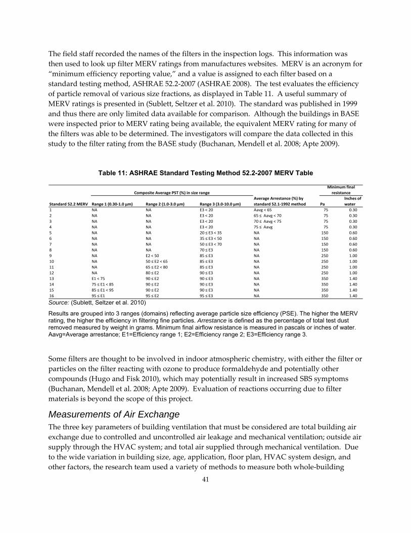
The field staff recorded the names of the filters in the inspection logs.  This information was then used to look up filter MERV ratings from manufactures websites.  MERV is an acronym for “minimum efficiency reporting value,” and a value is assigned to each filter based on a standard testing method, ASHRAE 52.2‐2007 (ASHRAE 2008).  The test evaluates the efficiency of particle removal of various size fractions, as displayed in Table 11.  A useful summary of MERV ratings is presented in (Sublett, Seltzer et al. 2010).  The standard was published in 1999 and thus there are only limited data available for comparison.  Although the buildings in BASE were inspected prior to MERV rating being available, the equivalent MERV rating for many of the filters was able to be determined. The investigators will compare the data collected in this study to the filter rating from the BASE study (Buchanan, Mendell et al. 2008; Apte 2009). 

 

Table 11: ASHRAE Standard Testing Method 52.2-2007 MERV Table

Standard 52.2 MERV Range 1 (0.30‐1.0 µm) Range 2 (1.0‐3.0 µm) Range 3 (3.0‐10.0 µm)Average Arrestance (%) by standard 52.1‐1992 method Pa

Inches of water

1 NA NA E3 < 20 Aavg < 65 75 0.302 NA NA E3 < 20 65 ≤  Aavg < 70 75 0.303 NA NA E3 < 20 70 ≤  Aavg < 75 75 0.304 NA NA E3 < 20 75 ≤  Aavg 75 0.305 NA NA 20 ≤ E3 < 35 NA 150 0.606 NA NA 35 ≤ E3 < 50 NA 150 0.607 NA NA 50 ≤ E3 < 70 NA 150 0.608 NA NA 70 ≤ E3 NA 150 0.609 NA E2 < 50 85 ≤ E3 NA 250 1.0010 NA 50 ≤ E2 < 65 85 ≤ E3 NA 250 1.0011 NA 65 ≤ E2 < 80 85 ≤ E3 NA 250 1.0012 NA 80 ≤ E2 90 ≤ E3 NA 250 1.0013 E1 < 75 90 ≤ E2 90 ≤ E3 NA 350 1.4014 75 ≤ E1 < 85 90 ≤ E2 90 ≤ E3 NA 350 1.4015 85 ≤ E1 < 95 90 ≤ E2 90 ≤ E3 NA 350 1.4016 95 ≤ E1 95 ≤ E2 95 ≤ E3 NA 350 1.40

Composite Average PST (%) in size rangeMinimum final resistance

Source: (Sublett, Seltzer et al. 2010)

Results are grouped into 3 ranges (domains) reflecting average particle size efficiency (PSE). The higher the MERV rating, the higher the efficiency in filtering fine particles. Arrestance is defined as the percentage of total test dust removed measured by weight in grams. Minimum final airflow resistance is measured in pascals or inches of water. Aavg=Average arrestance; E1=Efficiency range 1; E2=Efficiency range 2; E3=Efficiency range 3. Some filters are thought to be involved in indoor atmospheric chemistry, with either the filter or particles on the filter reacting with ozone to produce formaldehyde and potentially other compounds (Hugo and Fisk 2010), which may potentially result in increased SBS symptoms (Buchanan, Mendell et al. 2008; Apte 2009).  Evaluation of reactions occurring due to filter materials is beyond the scope of this project. 

Measurements of Air Exchange The three key parameters of building ventilation that must be considered are total building air exchange due to controlled and uncontrolled air leakage and mechanical ventilation; outside air supply through the HVAC system; and total air supplied through mechanical ventilation.  Due to the wide variation in building size, age, application, floor plan, HVAC system design, and other factors, the research team used a variety of methods to measure both whole‐building 

41 

 

 

ventilation rate and outside air flow supply rates. Numerous approaches have been developed for study of air exchange in commercial and residential buildings and are reported in the literature (Persily and Norford 1987; Turk 1989; Fisk, Faulkner et al. 1991; Fisk and Faulkner 1992; Fisk, Faulkner et al. 1993; ALNOR 1998; ASHRAE 1998; Fisk, Faulkner et al. 1998; Sherman 1998; Mendell, Fisk et al. 1999; ASTM 2000; Thatcher, McKone et al. 2001; ASHRAE 2002; McWilliams 2002; Wray, Walker et al. 2002; ASHRAE 2004; Persily and Gorfain 2004; Fisk, Faulkner et al. 2005; Wang 2005).  

One concern that has been raised is that different methods of ventilation measurement may yield systematically different results that could bias estimates of the distribution of SMCB ventilation rates.  For example, the BASE protocol applied three approaches and the agreement between them was poor (Persily, Gorfain et al. 2005).  However it is expected that the differences between the methods, if carefully executed will be small relative to the potentially large differences between buildings that meet existing standards and those that are out of compliance.   

Table 12 and Table 13  list the proposed methods, appropriate applications, and published standards and articles for all of these options.  Experts have used these methods in many situations for both residential and commercial building ventilation measurements, and most are included as recommended applications in ANSI (American National Standards Institute) and ASHRAE standards.  They are also further discussed in the sections below. 

Obtaining information on such important details as duct leakage to unconditioned spaces, or system balance, which are very important from the energy efficiency standpoint, was beyond the scope of this project.  Fortunately, this aspect of SMCB heating, ventilation, and air‐conditioning performance has been covered by others (Jacobs and Higgins 2003). 

Measurements of Whole Building Ventilation During the pilot portion of the study, which included the first five buildings, the goal was to measure the whole‐building ventilation using four different methods.  

The first method was to measure concentrations of a perfluorocarbon tracer gas (PFT) that had been released at a constant rate into the building in the occupied area for several days prior to the sampling day, such that the concentrations had come to steady state.  This method, referred to as the steady‐state method, was employed in all of the study buildings. 

This method utilizes a number of calibrated miniature PFT sources that are placed throughout the space.  They emit PFT at a constant and known rate, and are placed in sufficient number to generate a measurable concentration. 

The effective steady outside air flow rate can be computed from the measured tracer gas concentration and the tracer gas emission rates.  This is equivalent to the time‐invariant rate of outside air supply that would result in the measured tracer gas concentration if the indoor air were thoroughly mixed.  The equation for the effective steady outside air flow rate, Qwb is 

 42 

 

 

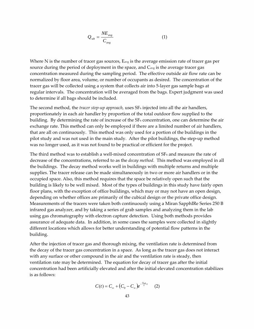
avg

avgwb C

NEQ =         (1) 

 

Where N is the number of tracer gas sources, Eavg is the average emission rate of tracer gas per source during the period of deployment in the space, and Cavg is the average tracer gas concentration measured during the sampling period.  The effective outside air flow rate can be normalized by floor area, volume, or number of occupants as desired.  The concentration of the tracer gas will be collected using a system that collects air into 5‐layer gas sample bags at regular intervals.  The concentration will be averaged from the bags. Expert judgment was used to determine if all bags should be included.   

The second method, the tracer step‐up approach, uses SF6 injected into all the air handlers, proportionately in each air handler by proportion of the total outdoor flow supplied to the building.  By determining the rate of increase of the SF6 concentration, one can determine the air exchange rate. This method can only be employed if there are a limited number of air handlers, that are all on continuously.  This method was only used for a portion of the buildings in the pilot study and was not used in the main study.  After the pilot buildings, the step‐up method was no longer used, as it was not found to be practical or efficient for the project.   

The third method was to establish a well‐mixed concentration of SF6 and measure the rate of decrease of the concentrations, referred to as the decay method.  This method was employed in all the buildings.  The decay method works well in buildings with multiple returns and multiple supplies. The tracer release can be made simultaneously in two or more air handlers or in the occupied space. Also, this method requires that the space be relatively open such that the building is likely to be well mixed.  Most of the types of buildings in this study have fairly open floor plans, with the exception of office buildings, which may or may not have an open design, depending on whether offices are primarily of the cubical design or the private office design.  Measurements of the tracers were taken both continuously using a Miran SapphIRe Series 250 B infrared gas analyzer, and by taking a series of grab samples and analyzing them in the lab using gas chromatography with electron capture detection.  Using both methods provides assurance of adequate data.  In addition, in some cases the samples were collected in slightly different locations which allows for better understanding of potential flow patterns in the building.  

After the injection of tracer gas and thorough mixing, the ventilation rate is determined from the decay of the tracer gas concentration in a space.  As long as the tracer gas does not interact with any surface or other compound in the air and the ventilation rate is steady, then ventilation rate may be determined.  The equation for decay of tracer gas after the initial concentration had been artificially elevated and after the initial elevated concentration stabilizes is as follows: 

( ) tVwbQ

eCCCtC −∞∞ −+= 0)(   (2) 

43 

 

 

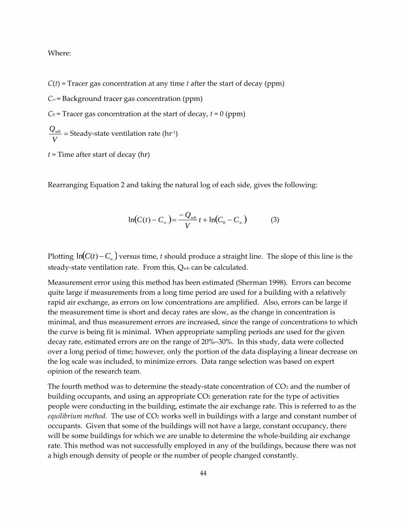
Where: 

 

C(t) = Tracer gas concentration at any time t after the start of decay (ppm) 

C∞ = Background tracer gas concentration (ppm) 

C0 = Tracer gas concentration at the start of decay, t = 0 (ppm) 

=V

Qwb Steady‐state ventilation rate (hr‐1) 

t = Time after start of decay (hr) 

 

Rearranging Equation 2 and taking the natural log of each side, gives the following: 

 

( ) ( ∞∞ −+ )−=− CCt

VQCtC wb

0ln)(ln   (3) 

 

Plotting  ( )∞−CtC )(ln  versus time, t should produce a straight line.  The slope of this line is the steady‐state ventilation rate.  From this, Qwb can be calculated. 

Measurement error using this method has been estimated (Sherman 1998).  Errors can become quite large if measurements from a long time period are used for a building with a relatively rapid air exchange, as errors on low concentrations are amplified.  Also, errors can be large if the measurement time is short and decay rates are slow, as the change in concentration is minimal, and thus measurement errors are increased, since the range of concentrations to which the curve is being fit is minimal.  When appropriate sampling periods are used for the given decay rate, estimated errors are on the range of 20%–30%.  In this study, data were collected over a long period of time; however, only the portion of the data displaying a linear decrease on the log scale was included, to minimize errors.  Data range selection was based on expert opinion of the research team.   

The fourth method was to determine the steady‐state concentration of CO2 and the number of building occupants, and using an appropriate CO2 generation rate for the type of activities people were conducting in the building, estimate the air exchange rate. This is referred to as the equilibrium method.  The use of CO2 works well in buildings with a large and constant number of occupants.  Given that some of the buildings will not have a large, constant occupancy, there will be some buildings for which we are unable to determine the whole‐building air exchange rate. This method was not successfully employed in any of the buildings, because there was not a high enough density of people or the number of people changed constantly. 

44 

 

 

This method is very similar mathematically to the tracer equilibrium method, except that rather than having a measured source rate of tracer gas, there is a calculated source of CO2 based on the number of occupants and a typical source rate per person.  The measurements will be made over a period of time for which there is fairly constant occupancy. 

 

The equation for the effective steady outside air flow rate, Qwb is: 

 

avgCO

COwb C

ENPQ_2

2×=         (4) 

 

Where NP is the number of people, ECO2 is the typical per‐person emission rate of CO2, and C CO2_avg is the average CO2 concentration measured during the period.   

Tracer decay methods are considered state of the art and have been used in numerous studies of commercial buildings (Cummings, Withers et al. 1996; Sherman 1998; McWilliams 2002; U.S. EPA 2003). 

One concern that has been raised is that different methods of ventilation measurement may yield systematically different results that could bias estimates of the distribution of SMCB ventilation rates.  To address this concern, summary statistics for each method are compared, and individual measurements of the PFT steady‐state and tracer decay methods are plotted against each other. 

Measurements of Mechanically Supplied Air There are two measures associated with mechanical supply of air: (1) the total supply flow rate into the building, including both re‐circulated and outdoor air, and (2) the flow rate of outdoor air supplied through the mechanical system intake. 

Total Supply Flow Rate Tracer Gas Airflow Measurement System (TRAMS, U.S. Patent #7,207,228) (Wang 2005) is the primary method for determining total air flow (Figure 2).  This method uses CO2 injected into the system return grille or the outside air intake at the air handler to measure the total air flow being supplied by a given air handler. This method was employed in most of the buildings. 

The TRAMS method is useful for measuring air flow in ducts where other methods are either impractical or less accurate.  It consists of injecting a known quantity of CO2 at a high rate and immediately mixes CO2 as a tracer into the supply duct.  Carbon dioxide increase in the duct is measured using an accurate and calibrated nondispersive infrared sensor (NDIR) real‐time monitor downstream of the injection point.  The measured dilution of CO2 by the supply air can be used to calculate the total supply flow rate. The TRAMS method of measuring airflow in a duct is very accurate, typically producing errors less than 5 percent.  The TRAMS method can 

45 

 

 

46 

ough 

ct, and the mass of the injected CO2 is determined by the is 

ically supplied air is: 

also be used by injecting CO2 into the return grille and measuring the concentration in the supply vent.  This approach must be taken in cases where there is not a sufficiently long ensupply duct, as is generally the case in SMCBs.  This approach underestimates the actual flow due to losses of CO2 in the exhaust.  The percent underestimation is comparable to the percent of outdoor air in the supply line.   

Carbon dioxide is injected in the dudifference of weights before and after injection.  Downstream of the injection location, the air sampled with an EGM‐4 carbon dioxide sensor (PP Systems, Amesbury, Massachusetts).  The EGM‐4 claims a 1 percent accuracy in CO2 measurement.  The EGM‐4 is connected to a computer that records data approximately every 1.6 seconds.  The data are stored in a spreadsheet program that performs the calculations listed below. 

The primary equation used to compute the total volume of mechan

 

ρTCCmQTMS )(

1000

0−=         (5) 

Where: 

TMS = Total volumetric flow rate of mechanically supplied air (m3/s) 

2

 

Q

m = Mass of injected CO  (g) 

C  = Average CO2 Concentration (ppm) 

C0  CO  = Background  2 concentration (ppm)

T = Time of integration (s) 

ρ  = Density of CO  in kilo2 grams/m3  (1.83) 

 

 arithmetic average of the CO2 concentration is obtained through numeric integration.  

ts 

ly 

 team measured the air flow through each supply and return grille 

The

In some cases, the TRAMS method was only able to be completed on a portion of the air handling system, either because there were too many air handlers or because some of uniwere configured such that they could not be accessed.  Also, many times for buildings with multiple air handlers, it was not possible to determine which air handler served which suppand return grille.   

In some cases, the researchusing a balometer. This method was impractical in most of the buildings because there were 

 

 

simply too many registers, or the supply and return grilles were inaccessible.  It was generally not used if flow could be measured using TRAMS. 

The actual air flow volume is directly measured for each supply vent.  If all supply vents are measured, the total air supplied is: 

 

∑=

=n

SVSVTMS QQ

1

        (6) 

 

Where QSV is the volumetric flow through a single supply vent, and n is the total number of supply vents. 

Outdoor Air Supply through Mechanical Ventilation  The research team made direct measurements of the mechanically supplied outdoor air intake primarily using a Duct Blaster®.  This method can only be used in buildings employing mechanically supplied outdoor air through a rooftop intake.  In limited cases the outdoor air supply flow exceeded the capacity of the Duct Blaster and a calibrated blower door fan was used in the same manner as the Duct Blasters.  In a limited number of cases when a Duct Blaster could not be used, a balometer was used to measure flow. 

The actual air flow volume is directly measured for each Duct Blaster.  If all Duct Blasters are measured, the total volume of outdoor mechanically supplied air is: 

 

∑=

=n

DBDBOMS QQ

1

       (7) 

 

Where QDB is the volumetric flow through a single duct blaster, and n is the total number of Duct Blasters. 

 

 

47 

 

 

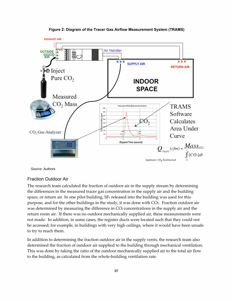
48 

 

Figure 2: Diagram of the Tracer Gas Airflow Measurement System (TRAMS)

Source: Authors

Fraction Outdoor Air The research team calculated the fraction of outdoor air in the supply stream by determining the differences in the measured tracer gas concentration in the supply air and the building space, or return air. In one pilot building, SF6 released into the building was used for this purpose, and for the other buildings in the study, it was done with CO2.  Fraction outdoor air was determined by measuring the difference in CO2 concentrations in the supply air and the return room air.  If there was no outdoor mechanically supplied air, these measurements were not made.  In addition, in some cases, the register ducts were located such that they could not be accessed; for example, in buildings with very high ceilings, where it would have been unsafe to try to reach them.  

In addition to determining the fraction outdoor air in the supply vents, the research team also determined the fraction of outdoor air supplied to the building through mechanical ventilation.  This was done by taking the ratio of the outdoor mechanically supplied air to the total air flow to the building, as calculated from the whole‐building ventilation rate.  

 

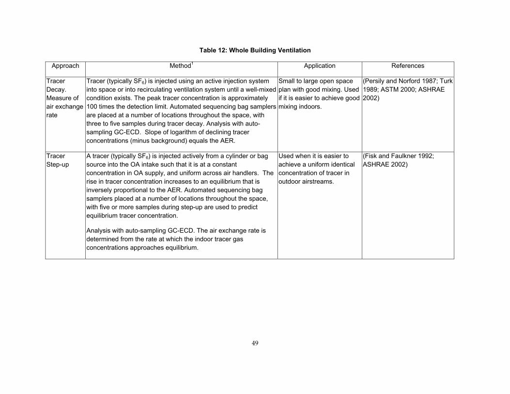
Table 12: Whole Building Ventilation

Approach Method1 Application References

Tracer Decay. Measure of air exchange rate

Tracer (typically SF6) is injected using an active injection system into space or into recirculating ventilation system until a well-mixed condition exists. The peak tracer concentration is approximately 100 times the detection limit. Automated sequencing bag samplers are placed at a number of locations throughout the space, with three to five samples during tracer decay. Analysis with auto-sampling GC-ECD. Slope of logarithm of declining tracer concentrations (minus background) equals the AER.

Small to large open space plan with good mixing. Used if it is easier to achieve good mixing indoors.

(Persily and Norford 1987; Turk 1989; ASTM 2000; ASHRAE 2002)

Tracer Step-up

A tracer (typically SF6) is injected actively from a cylinder or bag source into the OA intake such that it is at a constant concentration in OA supply, and uniform across air handlers. The rise in tracer concentration increases to an equilibrium that is inversely proportional to the AER. Automated sequencing bag samplers placed at a number of locations throughout the space, with five or more samples during step-up are used to predict equilibrium tracer concentration.

Analysis with auto-sampling GC-ECD. The air exchange rate is determined from the rate at which the indoor tracer gas concentrations approaches equilibrium.

Used when it is easier to achieve a uniform identical concentration of tracer in outdoor airstreams.

(Fisk and Faulkner 1992; ASHRAE 2002)

 

49 

 

 

 

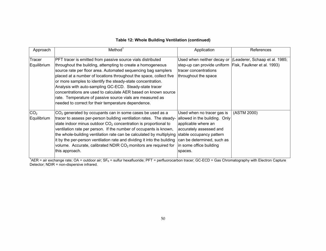
Table 12: Whole Building Ventilation (continued)

Approach Method1 Application References

Tracer Equilibrium

PFT tracer is emitted from passive source vials distributed throughout the building, attempting to create a homogeneous source rate per floor area. Automated sequencing bag samplers placed at a number of locations throughout the space, collect five or more samples to identify the steady-state concentration. Analysis with auto-sampling GC-ECD. Steady-state tracer concentrations are used to calculate AER based on known source rate. Temperature of passive source vials are measured as needed to correct for their temperature dependence.

Used when neither decay or step-up can provide uniform tracer concentrations throughout the space

(Leaderer, Schaap et al. 1985; Fisk, Faulkner et al. 1993)

CO2 Equilibrium

CO2 generated by occupants can in some cases be used as a tracer to assess per-person building ventilation rates. The steady-state indoor minus outdoor CO2 concentration is proportional to ventilation rate per person. If the number of occupants is known, the whole-building ventilation rate can be calculated by multiplying it by the per-person ventilation rate and dividing it into the building volume. Accurate, calibrated NDIR CO2 monitors are required for this approach.

Used when no tracer gas is allowed in the building. Only applicable where an accurately assessed and stable occupancy pattern can be determined, such as in some office building spaces.

(ASTM 2000)

1AER = air exchange rate; OA = outdoor air; SF6 = sulfur hexafluoride; PFT = perfluorocarbon tracer; GC-ECD = Gas Chromatography with Electron Capture Detector; NDIR = non-dispersive infrared.  

50 

 

 

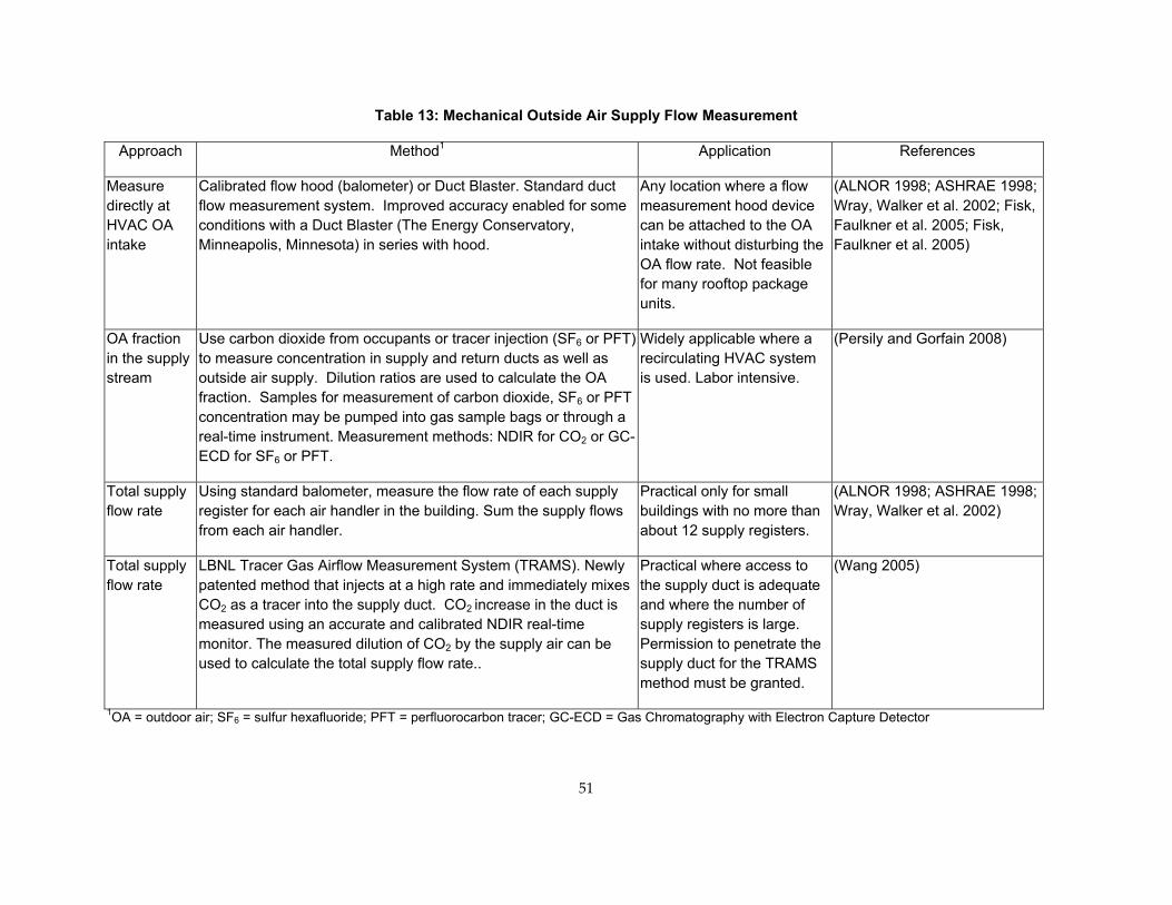
51 

 

Table 13: Mechanical Outside Air Supply Flow Measurement

Approach Method1 Application References

Measure directly at HVAC OA intake

Calibrated flow hood (balometer) or Duct Blaster. Standard duct flow measurement system. Improved accuracy enabled for some conditions with a Duct Blaster (The Energy Conservatory, Minneapolis, Minnesota) in series with hood.

Any location where a flow measurement hood device can be attached to the OA intake without disturbing the OA flow rate. Not feasible for many rooftop package units.

(ALNOR 1998; ASHRAE 1998; Wray, Walker et al. 2002; Fisk, Faulkner et al. 2005; Fisk, Faulkner et al. 2005)

OA fraction in the supply stream

Use carbon dioxide from occupants or tracer injection (SF6 or PFT) to measure concentration in supply and return ducts as well as outside air supply. Dilution ratios are used to calculate the OA fraction. Samples for measurement of carbon dioxide, SF6 or PFT concentration may be pumped into gas sample bags or through a real-time instrument. Measurement methods: NDIR for CO2 or GC-ECD for SF6 or PFT.

Widely applicable where a recirculating HVAC system is used. Labor intensive.

(Persily and Gorfain 2008)

Total supply flow rate

Using standard balometer, measure the flow rate of each supply register for each air handler in the building. Sum the supply flows from each air handler.

Practical only for small buildings with no more than about 12 supply registers.

(ALNOR 1998; ASHRAE 1998; Wray, Walker et al. 2002)

Total supply flow rate

LBNL Tracer Gas Airflow Measurement System (TRAMS). Newly patented method that injects at a high rate and immediately mixes CO2 as a tracer into the supply duct. CO2 increase in the duct is measured using an accurate and calibrated NDIR real-time monitor. The measured dilution of CO2 by the supply air can be used to calculate the total supply flow rate..

Practical where access to the supply duct is adequate and where the number of supply registers is large. Permission to penetrate the supply duct for the TRAMS method must be granted.

(Wang 2005)

1OA = outdoor air; SF6 = sulfur hexafluoride; PFT = perfluorocarbon tracer; GC-ECD = Gas Chromatography with Electron Capture Detector

 

Carbon Dioxide Measurements Carbon dioxide concentrations were measured both indoors and outdoors using Fuji Model ZFP‐9 NDIR monitors.  It should be noted that the TRAMS method injects CO2 into the building, raising the concentration.  Prior to any summary statistics being calculated with this data, the portion of the data influenced by TRAMS carbon dioxide injections was removed. 

This method has been used in studies conducted by LBNL and was sensitive enough to determine levels in buildings (Apte, Norman et al. 2008). 

Summary statistics are calculated for each building and across the set of buildings.  Real‐time concentrations were also averaged over each hour as well.  The average hourly and daily indoor/outdoor ratios are also reported. 

The research team compared concentrations to two types of standards, as introduced in the Background section of this report.  First, the research team compared  CO2 concentrations to the OSHA health standard of 5000 ppmV (parts per million volume) (OSHA 1994).  The research team also compared  CO2 concentrations to those specified in Title 24, a standard set to define sufficient ventilation using demand control ventilation, which is where CO2 concentration does not exceed 600 ppmV above the outdoor concentration (nominally defined as 400 ppmV if it is not measured (CEC 2008).  This is similar to the standard as set in ASHRAE 62.1, which is a steady‐state CO2 concentration of 700 ppmV above the outdoor level, assuming outdoor levels typically vary between 300 and 500 ppmV (ASHRAE 2007).  The maximum average concentration in the building should be used for comparison to the standard.  It is noted that when only one or two samplers are used, one cannot say it is a true building average concentration, as there is the potential for influence from local sources, such as a group of people standing near the sampler and talking.  As an alternative to the maximum concentration from an individual sampler, the 95th percentile may be an appropriate point on the distribution for comparison. 

Temperature and Relative Humidity The research team measured temperature and relative humidity conditions using Onset HOBO® U10 Temperature Relative Humidity data loggers, and collected additional temperatures using HOBO Pro V2 Internal and External Temperature Data Loggers. Summary statistics are calculated for each building and across the set of buildings.  The research team compared the levels with the comfort levels described in ASHRAE Standard 55, as introduced in the Background section of this report.  The standard is defined in terms of operative temperature, which is the sum of the ambient temperature and a measure of the effectiveness of the incident radiant heating on occupants (ASHRAE 2009).  For simplicity, the research team compared the ambient temperature to the standard as prescribed for the operating temperature. The summertime comfort standard is based on the assumption that people will be wearing a short‐sleeve shirt and cotton pants, while the wintertime standard is based on the assumption that people will be wearing a business suit.  There are not clear time periods where the standard should be applied.  However, since some portions of the state tend to be warmer or cooler, the 

52 

 

 

date one should switch from one standard to another in practice should vary throughout the State.  

Indoor Air Quality

Criteria Air Pollutants Carbon Monoxide Indoor carbon monoxide (CO) concentrations were measured using TSI Q‐track monitors.  The intent of CO monitoring was only to identify unusually high concentrations (e.g., > 5 ppmV); the lower limit of quantification of Q‐track monitors does not facilitate measurement of low concentrations.  This limitation is acceptable because determining concentrations at low levels is not a high priority.  Summary statistics are calculated for each building. One known problem with this monitor is that there can be a slight drift over time.  However, as noted above, since the primary reason for determining if the building is likely to be a problem building, this level of drift did not prevent us from meeting our objective.   

Real-Time Particle Concentrations Real‐time particulate matter (PM) concentrations with six different size fractions were measured using Met One 237AB instruments at each designated sample location for the building. The number of particles between two size fractions can be determined by difference.  After these calculations, the number of particles in each of the following size fractions is known:  0.3 to 0.5 μm, 0.5 to 0.7 μm, 0.7 to 1.0 μm, 1.0 to 2.0 μm, 2.0 to 5.0 μm, and 5.0 μm, and up. 

To determine if there were differences between the instruments, the research team co‐located samplers several times during the study.  If the differences between samplers in a given size fraction were below ±20 percent, the precision was considered acceptable and no adjustments were made.  If differences were too great, results were adjusted as discussed in the Quality Assurance/Quality Control (QA/QC) section of the results. 

The research team calculated PM mass concentration (PMmass) at each size fraction based on corrected PM count (PMcount) using the following equation: 

tqd

PMPM countmass 6][][

3π×=

ρ         (8) 

where particle density, ρ, is assumed to be 1 gram per cubic centimeter (g/cm3); particle diameter, d, is the average diameter of a size range  in μm (e.g., the average diameter for PM size fraction 0.3 to 0.5 μm is considered 0.4 μm and the diameter for PM size fraction 0.5 to 0.7 μm is considered 0.6 μm); sampling flow rate, q, is 2.8 liters per minute; and sampling time, t, is 40 seconds per minute. Final PM mass is presented in micrograms per cubic meter (μg/m3). 

PM2.0 was calculated by summation of all the size fractions up to this value. As calculations are made using the mid‐point and using a density of 1 g/cm3, both of which underestimate the actual mass concentration, plots presented in this report should be considered only to 

53 

 

 

understand the temporal profile, the relative contribution of the various size fractions, and the differences between indoor and outdoor levels, not as a measure of absolute values. 

Laser‐based optical particle counters (Model 237B, Met One, Grants Pass, Oregon) have been used in previous studies (Fisk, Faulkner et al. 2000).  Optical particle counters will undercount particles when concentrations are high, due to a tendency for multiple particles passing through the laser beam to be counted as a single particle. For the Met One counters, this undercounting due to coincidence loss (based on information from the manufacturer) is less than 10 percent at a total particle count of 140 particles per cubic centimeter).  

Integrated Particle Mass Concentrations Two 30 liter per minute (L/min) Harvard Cascading Impactors were used at each sample location, one collecting PM2.5 onto a filter and one collecting PM10 onto a Teflon filter (Demokritou, Gupta et al. 2002; Demokritou, Lee et al. 2004).  These impactors include multiple stages, each stage collecting particulate matter of different size fractions onto a small piece of polyurethane foam (PUF), with the final, smallest size fraction collected onto a Teflon filter.  The initial intent of this study was to quantify multiple size fractions gravemetrically, and the Harvard sampler was preferred for the short sampling periods expected in this study in order to maximize the number of samples that would be above the detection limit.  Another sampler that could measure multiple size fractions was available; however, based on the evaluation of that sampler, this project’s researchers had some concerns that there may be particle bounce from one filter media to the next as the sampler measured higher concentrations of small particles compared to the MOUDI sampler (Singh, Misra et al. 2003).  Particle bounce is unlikely to occur with the PUFmaterial. 

Initially, there were several deviations to this protocol.  During the pilot phase for Buildings 1 and 2, the PM2.5 mass was collected on multiple stages that were summed to determine PM2.5 and PM10.  Accurately determining the mass on multiple stages is problematic indoors due to the low concentrations, and these results are not considered very accurate.  For Building 3, only PM2.5 concentrations were collected.  For buildings 5 and 6, PM2.5 mass was captured on one filter, while PM10 measurements were determined by summing the mass on the PM2.5  filter with the mass on the PUF from the stage measuring PM2.5‐10. Blank samples and duplicate samples were collected.

Ultrafine Particle Concentrations Two portable condensation particle counters (CPC), Model 3781 (TSI, Shoreview, Minnesota) were employed for the major portion of the study. The Model 3781 uses water vapor to enlarge particles for easy detection by an optical detector. It can detect particles down to 6 nanometers (nm) in diameter. It has fast response to changes in aerosol concentration (< 2s to 95 percent in response to concentration step change). It measures particle concentrations up to 50,000 particles/cm3, and the accuracy for concentrations at 50,000 particles/cm3 is stated by the manufacturer to be within ±10 percent. It has an external power supply and can be left on unattended operation for one week. The feedback‐controlled, pressure‐corrected aerosol flow rate is 0.12 L/min. The internal data logger with user‐selectable data averaging ranges from 

54 

 

 

1 second to 1 hour. Various models of TSI condensation particle counter (CPC) samplers have been used in a number of past studies and use of TSI CPC samplers is considered a standard method for measuring ultrafine particulate matter(Weichenthal, Dufresne et al. 2007; Sotiriou, Ferguson et al. 2008; Weichenthal, Dufresne et al. 2008; Buonanno, Morawska et al. 2010; Koivisto, Hussein et al. 2010; Zhang, Gangupomu et al. 2010; Mullen, Bhangar et al. 2011; Wallace and Ott 2011). The portable P‐Track model provides lower accuracy than the model used here (Sarnat, Demokritou et al. 2003). For each building, indoor and outdoor particle counts are plotted.  Concentrations were recorded each minute and plotted as 10‐minute moving averages.   

To determine if there were differences between the instruments, samplers were co‐located several times.  If the differences between samplers in a given size fraction were below ±20 percent, the precision was considered acceptable and no adjustments were made.  If differences were too great, results were adjusted, as discussed in the QA/QC portion of the results 

Toxic Air Contaminants Toxic air contaminant (TAC) samples were collected using time‐integrated active samplers.  Volatile organic compounds are collected onto multi‐bed sorbent tubes (P/N 012347‐005‐00; Gerstel or equivalent) with primary bed of Tenax‐TA® sorbent backed with a section of Carbosieve®. Prior to use, the sorbent tubes were conditioned by helium purge (~10 cubic centimeters per minute [cc/min]) at 275°C (527°F) for 60 minutes and sealed in Teflon‐capped tubes. A set of dedicated tubes were used for this project. Drive MFlex L/S Modular 115V pumps (Cole‐Parmer) were used for sampling. Specifics of the sample collection and analysis can be found in the project plan. 

The list of target compounds is provided in Table 14, where the analytes are sorted by chemical class.  These compounds were selected because they are of health concern and have been found in measurable levels in commercial buildings, or because they are examples of compounds that might not be as relevant for health endpoints but have been found in high concentrations in commercial buildings.  In addition, decamethyl‐cyclopentasiloxane (D‐5 Siloxane); hexane; diethyl phthalate; 2,2,4‐trimethyl‐1,3‐pentanediol diisobutyrate (TXIB); and hexanal were added to the list of quantified compounds. 

The VOC sample volume was five liters for the pilot study.  In some cases, the amount of chemical was above the quantifiable range, indicating that the sample volume was too high. On the other extreme, many compounds were below the limit of detection (LOD), particularly outdoors.  For the remainder of the project, a sample volume of 4 L indoors and 10 L outdoors was used. 

Specifically, VOCs were quantitatively analyzed by thermal‐desorption gas chromatography/mass spectrometry (TD‐GC/MS), generally following U.S. EPA Method TO‐17, which is considered a standard method (Woolfenden and McClenny 1997).  For quantitative analysis of the target compounds, multi‐point calibrations were created using pure compounds and 1‐bromo‐4‐fluorobenzene as an internal standard.  Sorbent tubes were thermally desorbed 

55 

 

 

for analysis using a thermodesorption auto‐sampler (Model TDSA2; Gerstel), a thermodesorption oven (Model TDS3, Gerstel), and a cooled injection system (Model CIS4; Gerstel). The cooled injection system was fitted with a Tenax‐packed glass liner (P/N 013247‐005‐00; Gerstel). Desorption was run in splitless mode at a starting temperature of 25°C (77°F) with a 0.5‐minute delay followed by a 60°C (140°F) ramp to 250°C (482°F) and a 4‐minute hold time. The cryogenic trap was held at ‐10°C (14°F) throughout desorption and then heated within 0.2 minutes to 270°C (518°F) at a rate of 12°C (54°F)/s, followed by a 3‐minute hold time. Compounds were resolved on a GC (Series 6890Plus; Agilent Technologies) equipped with a 30 meter HP‐1701 14 percent Cyanopropyl Phenyl Methyl column (Model 19091U‐233; Agilent Technologies) at an initial temperature of 1°C (34°F) for 0.5 minutes then ramped to 40°C (104°F) at 25°C (77°F)/min, to 115°C (239°F) at 3°C (37°F)/min, and finally to 250°C (482°F) at 10°C (50°F)/min, holding for 10 minutes.  The resolved analytes were detected using electron impact MS (5973; Agilent Technologies). The MS was operated in scan mode. All pure standards and analytes were referenced to the internal standard (~120 ng) of 1‐bromo‐4‐fluorobenzene.  

Formaldehyde, acetaldehyde and acetone were collected using a different method.  Samples were collected using U.S. EPA method TO11 – Method for the Determination of Formaldehyde in Ambient Air Using Adsorbent Cartridge Followed by High Performance Liquid Chromatography (Willbury, Tejada et al. 1999).  Sampling was conducted using a cartridge packed with silica gel that is coated with acidified 2,4‐dinitrophenylhydrazine (DNPH) (P/N WAT047205 from Waters Corp). Ozone scrubbers were used on all samples to prevent aldehyde loss due to reaction with ozone on the absorbent. Higher molecular weight aldehydes can be measured either by TO‐11 or TO‐17, but GC/MS is commonly used for detection and quantification whenever the option is available and is considered an acceptable method.  

Laboratory analysis of aldehyde samples involves elution with acetonitrile and analysis by high‐performance liquid chromatography (HPLC). Different DNPH‐derivatives elute at different retention times, depending mainly on their molecular size.  External standards were used to determine the mass of target compounds based on the peak area.  Extracts were analyzed by HPLC (1200 Series; Agilent Technologies) using a C18 reverse‐phase column with 65:35 H2O:  Acetonitrile mobile phase at 0.35 ml/min and ultraviolet detection at 360 nm. Multipoint calibrations were prepared for the target aldehydes using commercially available hydrazone derivatives of formaldehyde and acetaldehyde. 

The analytical methods for both VOCs and aldehydes are standard U.S. EPA methods that have been used in numerous studies (Woolfenden and McClenny 1997; Clayton, Pellizzari et al. 1999; Willbury, Tejada et al. 1999; Edwards, Jurvelin et al. 2001; Adgate, Church et al. 2004; Adgate, Eberly et al. 2004; Sax, Bennett et al. 2004; Sexton, Adgate et al. 2004; Sexton, Adgate et al. 2004; Liu, Zhang et al. 2006; Sax, Bennett et al. 2006; Dodson, Houseman et al. 2007).   

  

56 

 

 

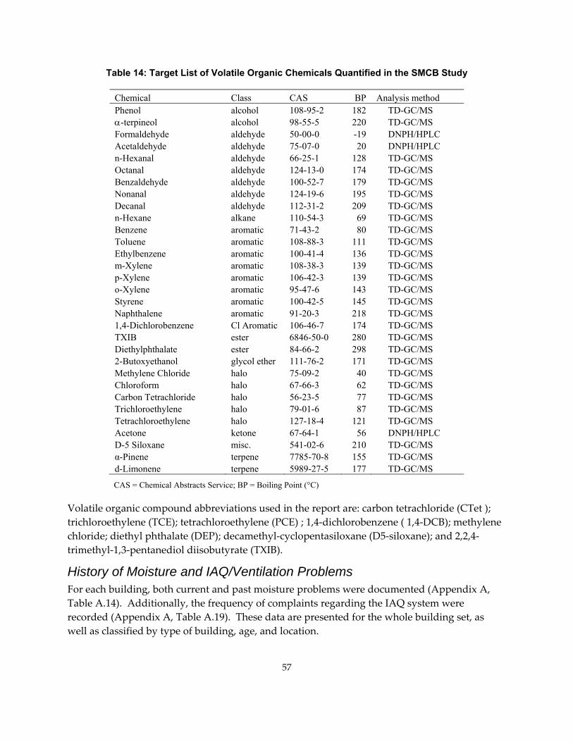
Table 14: Target List of Volatile Organic Chemicals Quantified in the SMCB Study

Chemical Class CAS BP Analysis method Phenol alcohol 108-95-2 182 TD-GC/MS α-terpineol alcohol 98-55-5 220 TD-GC/MS Formaldehyde aldehyde 50-00-0 -19 DNPH/HPLC Acetaldehyde aldehyde 75-07-0 20 DNPH/HPLC n-Hexanal aldehyde 66-25-1 128 TD-GC/MS Octanal aldehyde 124-13-0 174 TD-GC/MS Benzaldehyde aldehyde 100-52-7 179 TD-GC/MS Nonanal aldehyde 124-19-6 195 TD-GC/MS Decanal aldehyde 112-31-2 209 TD-GC/MS n-Hexane alkane 110-54-3 69 TD-GC/MS Benzene aromatic 71-43-2 80 TD-GC/MS Toluene aromatic 108-88-3 111 TD-GC/MS Ethylbenzene aromatic 100-41-4 136 TD-GC/MS m-Xylene aromatic 108-38-3 139 TD-GC/MS p-Xylene aromatic 106-42-3 139 TD-GC/MS o-Xylene aromatic 95-47-6 143 TD-GC/MS Styrene aromatic 100-42-5 145 TD-GC/MS Naphthalene aromatic 91-20-3 218 TD-GC/MS 1,4-Dichlorobenzene Cl Aromatic 106-46-7 174 TD-GC/MS TXIB ester 6846-50-0 280 TD-GC/MS Diethylphthalate ester 84-66-2 298 TD-GC/MS 2-Butoxyethanol glycol ether 111-76-2 171 TD-GC/MS Methylene Chloride halo 75-09-2 40 TD-GC/MS Chloroform halo 67-66-3 62 TD-GC/MS Carbon Tetrachloride halo 56-23-5 77 TD-GC/MS Trichloroethylene halo 79-01-6 87 TD-GC/MS Tetrachloroethylene halo 127-18-4 121 TD-GC/MS Acetone ketone 67-64-1 56 DNPH/HPLC D-5 Siloxane misc. 541-02-6 210 TD-GC/MS α-Pinene terpene 7785-70-8 155 TD-GC/MS d-Limonene terpene 5989-27-5 177 TD-GC/MS

CAS = Chemical Abstracts Service; BP = Boiling Point (°C)

Volatile organic compound abbreviations used in the report are: carbon tetrachloride (CTet ); trichloroethylene (TCE); tetrachloroethylene (PCE) ; 1,4‐dichlorobenzene ( 1,4‐DCB); methylene chloride; diethyl phthalate (DEP); decamethyl‐cyclopentasiloxane (D5‐siloxane); and 2,2,4‐trimethyl‐1,3‐pentanediol diisobutyrate (TXIB). 

History of Moisture and IAQ/Ventilation Problems For each building, both current and past moisture problems were documented (Appendix A, Table A.14).  Additionally, the frequency of complaints regarding the IAQ system were recorded (Appendix A, Table A.19).  These data are presented for the whole building set, as well as classified by type of building, age, and location. 

57 

 

 

Two variables on moisture damage were created.  The first is a yes/no variable for current moisture damage; the second is a yes/no variable for current or past water damage.  T‐tests were used to compare continuous ventilation rates and overall inspection scores between those buildings with moisture damage and those without. 

The questionnaire included a section regarding building occupant complaints related to the indoor environment, such as complaints about temperature, stuffiness, or odors. Respondents were specifically asked if the building environment was too hot in the warm season, too hot in the cool season, too cold in the warm season, too cold in the cool season, or too drafty. They were also asked if there was too little air movement, if there were odors, or if they had other complaints. In addition, they were asked about the frequency of these complaints (daily, weekly, monthly, quarterly, annually, once, or never). For analysis of this section, responses were grouped to the above complaint questions into three general frequency categories (frequent, infrequent, and never). The “daily,” “weekly,” and “monthly” responses were categorized as “frequent” complaints; the “quarterly,” “annually,” and “once” responses were categorized as “infrequent” complaints; and participants who reported “never” for a particular complaint were categorized as such. A variable was created specifying the frequency of any temperature‐related complaint (frequent, infrequent, or never). 

Comparisons to results from the telephone survey of SMCB in California were made (Piazza and Apte 2010). 

Particle Infiltration Indoor and outdoor semi‐continuous measurements of black carbon were collected using Aethalometers®, allowing for determination of the fraction of outdoor particles of comparable size likely reaching the indoor environment.   

Particles of outdoor origin enter buildings through purposeful openings such as doors and windows, as well as through cracks and crevices in the building envelope.  As particles travel through the cracks, they can be removed by impaction, diffusion, or interception mechanisms.  The fraction of particles removed by these different mechanisms varies by particle size as the relative inertia and drag forces vary by particle size.  The penetration efficiency (P), the fraction of particles of a specific diameter that pass through the building envelope, is dependent on the number and geometry of the cracks, as well as the velocity of the air passing through the cracks, which is a function of the air exchange rate (Liu and Nazaroff 2001).  The roughness and shape of the crack are also influential (Jeng, Kindzierski et al. 2006; Jeng, Kindzierski et al. 2007; Tian, Zhang et al. 2008).  It is expected that particle losses vary by building, due to differences in building characteristics, suggesting the need for taking measurements on a wide range of buildings.  Particle losses also vary temporally due to changes in air exchange rates, wind velocities, relative humidity, and temperature differences—suggesting the need for modeling results dynamically and understanding the impact of these factors.  The penetration efficiency is lower for small particle sizes (<0.1 μm), due to Brownian deposition, and for larger particles (>1.5 μm), due to impaction, interception and gravitational loses. Therefore, the different 

58 

 

 

particle size fractions of the regulated fine and coarse particle mass are not expected to exhibit the same penetration factors. 

Once in the building, particles are deposited onto indoor surfaces, and the rate of deposition is controlled by the deposition rate, k (1/h).  Again, this process is strongly influenced by particle size.  The deposition rates have been studied in homes and found to vary between homes due in part to differences in air flow velocities within the home, the quantity and surface of furnishings in the home, the interior surface‐to‐volume ratio, and the difference in temperature differential between the air and surfaces and particle roughness. These differences are likely in commercial buildings as well (Lai and Nazaroff 2000; Thatcher, Lai et al. 2002; Lai 2006). 

Due to penetration and deposition losses indoors, particle concentrations indoors are lower than outdoor concentrations in cases where there are no indoor sources.  The infiltration factor (Finf) has been defined as the fraction of outdoor particles that penetrate indoors and remain suspended (Wilson and Suh 1997; Wilson, Mage et al. 2000).  Therefore, determining infiltration efficiency and understanding its relationship to the different parameters such as building characteristics, air exchange rates, temperature, and other factors is very important in our efforts to assess individual and population exposures to particles of outdoor origin. These processes have been widely studied in homes.  For example, an infiltration factor was calculated by size fraction using a dynamic model for a number of homes (Bennett and Koutrakis 2006).  Available data from a large number of studies on infiltration, primarily in homes, have recently been summarized (Chen and Zhao 2011).   

Studies have also determined the infiltration factor by determining the indoor/outdoor ratio of particles thought to be of outdoor origin (Meng, Turpin et al. 2007).  One particle component that is primarily of outdoor origin is black carbon, primarily generated by motor vehicles; specifically diesel vehicles. 

In this study, indoor/outdoor (I/O) ratios were calculated for black carbon as measured by Aethalometers.  It is important to note that Aethalometers are not size specific, and thus the measured I/O ratio could vary by the relative size distribution of black carbon in the outdoor air, as particles of different size fractions have different infiltration rates. 

Three Aethalometers were used to measure black carbon, with one located on the roof (representing the concentrations brought in through the air handler), one located outside the building at ground level (representing concentrations brought in through the building shell), and one located indoors.  The model numbers of the samplers were AE22 and AE31—both full size instruments were used either in the indoor or outdoor locations—and a portable model, AE42, which was generally taken to the rooftop location.   

Concentrations were recorded every five minutes.  Negative values were removed from the dataset.  Data were averaged over a 30‐minute period, including all available data.  If data from one time period were missing, concentrations were calculated based on the average concentrations for the remaining time periods.  If more than one data point was missing, 

59 

 

 

concentrations were interpolated between the levels estimated just before and just after the period where data were not recorded.   

To determine if there were differences between the instruments, samplers were co‐located several times.  If the differences between Aethalometers were below ±20 percent, the precision was considered acceptable and no adjustments were made.  If differences were too great, results were adjusted, as discussed in the QA/QC section of this report. 

Data Analysis A statistical analysis plan was developed prior to conducting the field study, and it was reviewed and approved by the external review committee.  This document formed the basis for the analysis conducted in this report.  Where there were significant deviations from the planned methodology, it is noted below. 

For all statistical analysis, SAS statistical software, version 9.2 for Windows® (SAS Institute Inc., Cary, North Carolina) was used. 

Characterization of Physical Plant: Maintenance and Operation of Building, Focus on HVAC and Air Filtration Systems Creation of Overall Condition Variable The SMCB Inspection Log provides evaluations of several aspects of each building’s rooftop HVAC units. The inspection results of individual components of the HVAC system were grouped together and analyzed in an effort to evaluate the overall condition of various elements of the HVAC system, as well as the condition of the HVAC system as a whole.  

Supply/Return Fans: If all fans (supply and return) on the inspected rooftop units were operating, the building was assigned a value of 1. However, if one or more fans were nonoperational, the building was assigned a value of 2. The average score for the created FANOPER variable was calculated across all inspected buildings. Each individual building’s score was divided by the average score of all buildings to compute a normalized value (FANOPERNM) for the integrated fan operation variable. A normalized value of less than 1 indicates that all fans were operating, and values greater than one indicates that one or more fans were nonoperational across one or more rooftop units. 

For each of the following elements (listed below), the same basic scoring protocol was utilized. Each specific component comprising the various elements of the HVAC system was rated on a scale of 1 to 3, with a score of 1 equivalent to good condition, a score of 2 equivalent to an intermediate condition and a score of 3 equivalent to poor condition, with details listed in Table 10, above.  For each building with more than one rooftop unit inspected, the average score for each specific component was calculated across the rooftop units for the building. Then an average score was calculated across all of the inspected buildings. Next, each individual building’s score was divided by this overall average to compute a normalized value for each of the HVAC system elements. A normalized value of less than 1 indicated that each component 

60 

 

 

was in good or better condition, while scores above 1 indicated that the building had some deficiencies for at least one component. After the normalized scores were calculated for each component of a given element of the HVAC system, the average of all the normalized scores was calculated to create a normalized score for the HVAC system element overall, with the systems being listed below.  

Air Handling Units: Several components of the air handling units were inspected, including the general condition of the air handling unit housing, the air handling unit housing sound liner, the general condition of the air handling unit itself, the heating and cooling coils, the condensate drain pan, and the fan belts.  

Air Distribution Ductwork: The general condition of the air distribution ductwork, evaluation of leakage at sheet metal seams, and the ductwork liners were the components of the air distribution ductwork that were evaluated during the inspection. 

Particulate Filtration Systems: For the particulate filtration systems, the general condition of the system, the fit of the filters into their frames, the filter condition and the evenness of filter loading were inspected.  

Control System: The general condition of the control system and the condition of the sensors were inspected.  

After the normalized score for each element was determined, all scores across all elements were averaged to create an “overall” score for each building’s HVAC system.  A lower normalized value indicated that the building’s overall system was well maintained. 

Although a similar inspection process was used by the BASE study (U.S. EPA 2003), published data are not available for comparison. 

Summary statistics were determined for reported HVAC inspection frequency.  The results have been compared to those obtained by the SMCB phone survey (Piazza and Apte 2010).  While HVAC inspection frequency data were collected in BASE, the data have not been published and thus comparisons cannot be made. 

The research team compared the overall condition based on building characteristics and reported inspection frequency.  Where the distribution between two variables was compared, a t‐test was used to check for significance. Where multiple distributions were compared, an analysis of variance was used.  Least‐squares means and/or orthogonal contrasts were used to compare specific types 

The names of the filters in the inspection logs were used to determine filter MERV ratings from manufacturer websites.  Although the buildings in BASE were inspected prior to MERV rating being available, the equivalent MERV rating for many of the filters were able to be determined and the data collected in this study have been compared to that dataset (Buchanan, Mendell et al. 2008; Apte 2009). 

 61 

 

 

Accessibility of Filter The SMCB Inspection included an evaluation of the accessibility of a building’s particulate filtration system. The research team scored each of the RTUs that were investigated on a scale from 1 to 3, with a 1 indicating large access doors and adequate space for inspecting and changing filters, a 2 indicating small access doors and limited space for inspecting/changing filters, and a 3 indicating an absence of access doors and no means of inspecting or changing filters. The scores in this section were grouped in the following manner to create an overall assessment of the accessibility of the particulate filtration system: buildings with a score of 1 for all RTUs were generally categorized as having “easy access,” buildings with only scores of 2 or 3 across the RTUs were categorized as “difficult access,” and buildings with mixed scores of 1s together with 2s or 3s were categorized as “mixed access.”  Condition was evaluated for different levels of accessibility. There were no existing data available for comparison. 

Building Ventilation There are several parameters for describing building ventilation.  Whole building ventilation can be presented as (1) an air exchange rate, the rate at which the air in the entire building is replaced, as the total rate of air being delivered to the building, or (2) as an air supply rate, either per floor area or per person.  Each way of presenting the data is useful for different purposes.  The air exchange rate is conceptually easy to understand and is useful for comparing to residential rates, which are typically expressed in these units (Dodson, Levy et al. 2009).  The total rate of air being delivered to the building is easily understood by readers who are familiar with delivery rates of HVAC systems, as these are typically reported in terms of a total air delivery rate.  Relevant commercial building standards (Title 24 and ASHRAE 62.1) include both standards of air provided on a per‐person and a per‐area basis (CEC 2005; ASHRAE 2010).  Standards are needed on both a per‐person and a per‐area basis because for some contaminants of concern, the person can be considered to be the source (i.e., CO2 or odors) while the building area is relevant to consider for sources related to building materials, such as formaldehyde.  No one measure is considered superior to another overall, the reader needs to select which is most relevant for a specified comparison. 

Total mechanically supplied outdoor air is also presented in multiple ways, specifically as the total rate of air being delivered to the building, or as an air supply rate, either per floor area or per person.  The reasons for the multiple methods are the same as for total air supply to the building, and again, there is no preferred method. 

For each of the ventilation parameters measured, summary statistics are calculated. Methods for whole‐building ventilation are compared to determine the best one for use in the remainder of the analyses. Resulting distributions are compared to data available in the literature (Cummings, Withers et al. 1996; Persily and Gorfain 2004). 

Total mechanical air supplied to the building was either determined using the TRAMS method or by measurement through the supply vent.  In some buildings, only one method could be employed.  In some buildings, both methods were employed and can be compared.  Summary 

62 

 

 

statistics from the two methods were determined and are presented separately.  Data from this study were compared to existing data from the BASE study (Persily and Gorfain 2004).   

Summary statistics were determined for the percent of outdoor air in the mechanically supplied air.  This gives the reader an idea of the percent of fresh air delivered in the supply stream. 

A very different percent was also determined: the estimated percent of outdoor air delivered mechanically.  This percent was calculated by dividing the mechanically supplied outdoor air as determined by the Duct Blaster measurements by the total amount of outdoor air supplied to the building.  This parameter helps the reader understand what fraction of the air is delivered through the HVAC system and what fraction is delivered through leakage of the building envelope or through natural ventilation. 

A series of factors that may be related to building ventilation rate, including building age, region, size, and use were evaluated.  The per‐area and per‐person ventilation rates were plotted against year, to determine potential age split. The research team divided the buildings into two groups by three age split criteria.  The first was pre‐ and post‐1983.  This year was selected because Title 24 was enacted in 1978, and it was thought that buildings were likely to have been implementing the standards by 1983.  Additional comparisons were made splitting the data at 1990 and 2000 for exploratory purposes.  A t‐test was used to determine if there were significant differences in the ventilation rate of the buildings by age group.  Finally, the research team conducted a regression analysis looking at the age of the building in years (a continuous variable) versus ventilation rate. 

Using the defined regions, northern‐coastal, northern‐inland, southern‐coastal, southern‐inland, or central‐inland, the research team used an analysis of variance to determine if significant differences in ventilation rates exist with respect to region. However, since no statistical significance was observed. The northern‐coastal region (which was cooler than other regions) was compared with the other four regions combined. 

Besides age and region, the research team also examined other factors (e.g., building use, size, ambient temperature, maintenance practices), and tested the associations between predictor variables and ventilation rate.  If predictor variables were significant at p<0.1 in single regressions, variables were included in a multiple regression model to analyze the relationship of these variables with respect to ventilation rate.  The number of variables included, as well as the possibility of interaction terms, was limited due to sample size restrictions. 

In addition, the research team compared buildings’ outside air flow rates to Title 24 standards on per‐person and per‐area basis, respectively.  Each building was classified as 20 percent higher than, 20 percent lower than, or within ±20 percent of the Title 24 standard for descriptive purposes, to look for trends among building groups. The statistical analysis plan specified determination of buildings that were significantly above or below the standard, and the research team determined that 20 percent above or below constituted a significant difference. The complete building dataset was stratified by building size (small/medium buildings versus medium and medium/large buildings), building age (before and after 1983, before and after 

63 

 

 

1990, and before and after 2000), and building use (offices, dental clinic/healthcare, retails/groceries, restaurants, other buildings). A chi‐square test, or if necessary, the Fisher’s Exact test, was used to examine if a building’s outside air flow rates (quantified as > 20 percent higher and lower than the Title 24 standards) was related to building size, age, and use.   

Criteria Air Pollutants The authors calculated summary statistics for all real‐time instruments for each building and the average concentrations of each building for both the whole set of buildings and for various building types.  Summary statistics were also calculated for integrated PM concentrations. Indoor/outdoor ratios, which are often calculated in studies of particulate matter and ultrafine particulate matter, were also calculated and presented. Measured concentrations were compared to concentrations found in previous studies for both PM 2.5 and ultrafine particulate matter (Sotiriou, Ferguson et al. 2008; Weichenthal, Dufresne et al. 2008; Buonanno, Morawska et al. 2010; Koivisto, Hussein et al. 2010; Mullen, Bhangar et al. 2011) and to health guidelines, where applicable. 

Based on potential sources, the authors classified the buildings into a specified building type from the following list: non‐medical office, grocery/restaurant, retail, dental office/hair salon, and other.  Grocery stores were included with restaurants because they had cooking located within them and sources related to cooking were thought to be important, justifying the combination of these two building types. 

The authors tested variability of indoor concentrations of PM between buildings with different functions, as listed above. An analysis of variance was test used to see for which compounds and building types significant differences occur.  Least‐squares means and/or orthogonal contrasts were used to compare specific types, as specified in the statistical analysis plan. 

Toxic Air Contaminants The research team measured a suite of toxic air contaminants at one or two indoor locations and at one outdoor location in each building.  The authors reviewed blanks to determine if there was any lab contamination and any affected samples were excluded. 

The authors calculated summary statistics for indoor measured concentrations, and then averaged the two indoor concentrations and calculated summary statistics.  These averaged indoor concentrations were then used in all additional calculations.  Summary statistics were also presented by building type.  Based on potential sources, the authors classified the buildings into a specified building type from the following list: non‐medical office, grocery/restaurant, retail, dental office/healthcare, gas/auto services, hair salon/gym, and other.  Indoor/outdoor differences and indoor/outdoor ratios were calculated. These measures have been reported in other studies (Edwards, Jurvelin et al. 2001; Sax, Bennett et al. 2004; Dodson, Levy et al. 2009). Values below detection limit were coded as zero when calculating indoor/outdoor differences and emission factors. 

64 

 

 

Measured concentrations were compared to health standards and to concentration ranges found in other studies of commercial buildings (Daisey, Hodgson et al. 1994; Girman, Hadwen et al. 1999; Hinwood, Berko et al. 2006; Hotchi, Hodgson et al. 2006; Loh, Houseman et al. 2006; Ongwandee, Moonrinta et al. 2009).  

The authors calculated indoor contaminant whole‐building source strength for each building, assuming a steady‐state, well‐mixed box model incorporating outdoor concentrations, air exchange rates, and building volumes. Building source strengths have been calculated in other studies, typically residential studies, as sufficient data to calculate building source strengths is typically not available in studies of commercial buildings (Zhang, He et al. 1994; Sax, Bennett et al. 2004; Liu, Zhang et al. 2006; Dodson, Levy et al. 2009). Sources are characterized by source strength estimates, also called whole‐building source strength, which have units of mass per time.  Whole‐building source strengths can be considered the apparent source strength for the combined mix of individual indoor sources, given the non‐ventilation loss mechanisms inherent in the building type.  Building source strengths can be estimated with the following steady‐state mass balance equation: 

S = aV iC − oC( )      (8) 

where a is the total air exchange rate of the building (h‐1), V is the volume of the building (m3), Ci is the measured concentration in the building for the specified compound (μg/m3), and Co is the measured concentration outside of the building for the specified compound (μg/m3).  These models assume that penetration of VOCs from the outdoors is one, as shown in previous work (Lewis 1991), and that losses by reaction are less than losses by air exchange since the time scale of decay is at most 1x10‐3 per hour for VOCs indoors compared with an air exchange rate of 0.1 to 1 per hour (Finlayson‐Pitts and Pitts Jr 1986).  In addition, the whole‐building source strength per area was calculated.  Summary statistics are presented for both measures across the entire dataset, and for the source strength per unit area, summary statistics are also calculated for each building type. 

The authors tested the variability of indoor concentrations of selected toxic air contaminants between buildings with different functions. An analysis of variance was used to test to see for which compounds and building types significant differences occur.  Least‐squares means and/or orthogonal contrasts were used to compare specific types. 

The hypothetical distribution of formaldehyde concentrations was determined based on the actual outdoor concentrations and building source strengths, combined with the air exchange rate based on the Title 24 value set on a per area basis.  The hypothetical indoor concentration was determined using the following equation: 

VaS

C oi24

24, C +=         (9) 

where Ci,24 is the hypothetical indoor concentration if air exchange were set at the value defined in Title 24 and a24 is the air exchange rate based on the Title 24 regulation value on a per area 

65 

 

 

basis (equal to the Title 24 air flow rate per area x area / volume). All other terms are defined above. 

The authors conducted source apportionment analysis on indoor VOC concentrations using the principal factor analysis technique (Loehlin 1992). Principal factor analysis was selected over principal component analysis because we assume a large portion of the variance of the concentrations was attributed to specific sources or activities in individual buildings, which may not be representative in all of the SMCBs serving various functions. Thus, using factor analysis, we analyzed the common variance of all the compounds to examine the inter‐correlations among the compounds.   

Factor analysis has been conducted on environmental samples for VOCs (Daisey, Hodgson et al. 1994; Heavner, Morgan et al. 1995; Kim, Harrad et al. 2001; Miller, Anderson et al. 2002; Logue, Small et al. 2009) and more widely for particle composition (Harrison, Smith et al. 1996; Kavouras, Koutrakis et al. 2001; Song, Polissar et al. 2001) for source apportionment purpose. Although with the limited number of observations from the sample of 40 buildings, the factor analysis may not be statistically valid, it could provide some idea on groupings of VOCs and identifying potential sources. Pearson correlation coefficients were first calculated based on log‐transformed indoor VOC concentrations to identify correlated compounds. After excluding correlated variables, factor analysis was conducted on log‐transformed indoor VOC concentrations.  If VOC concentrations were measured at two indoor locations within the building, the two locations are each included as separate data points in the analysis. Squared multiple correlation (SMC) between the variable and all other variables was used to estimate prior communalities. The residual correlation matrix and partial correlation matrix was evaluated to determine if the retained factors were sufficient to explain the correlations among the observed variables. Since the initial factor pattern matrix is not unique, an oblique rotation after an orthogonal VARIMAX rotation was performed to achieve more interpretable factor loadings. Factor loadings greater than 0.50 are considered to be significant in this analysis.  

Particle Infiltration The research team collected indoor, outdoor (~1 m above ground level), and roof concentrations of black carbon every 5 minutes continuously, and calculated a centered 30‐minute moving average for each recording point (±15‐minute intervals).  Two types of ratios were calculated: (1) An indoor/outdoor or indoor/roof ratio for each time period, matching the outdoor time to the indoor time, and (2) similar ratios, but with a time lag. Time lags of 10, 20, and 50 percent of the average age of air (namely, the inverse air exchange rate) in the building were considered. This method was proposed in the statistical analysis plan.  While the authors are unaware of this method being used in prior studies, it is based on theoretical considerations.  The differential mass balance equation defining the indoor concentration in the absence of indoor sources is: 

ininoutin kCaCaPC

dtdC

−−=     (10) 

66 

 

 

where Cin is the indoor concentration (mg/m3), Cout is the outdoor concentration (mg/m3), a is the air exchange rate (1/h), P is the penetration rate through the building shell (unitless), and k is the deposition rate (1/h).  Solving the equation numerically yields: 

tkCaCaPCC ttinttinttoutttintin Δ−−+= Δ−Δ−Δ−Δ− )(C ,,,,,  (11) 

As one can see from the above equation, Cin,t‐Δt is based on the outdoor and indoor concentrations at the previous time step.  The indoor concentration at the previous time step is in turn dependent on the outdoor concentration at two time steps prior and the indoor concentration at two time steps prior.  This pattern continues, such that the indoor concentration is dependent on the time‐averaged previous outdoor concentrations, and the averaging function is based on the value of a, P, and k, with the integrated time period increasing as a decreases.  As conducting an analysis of the dynamic data is beyond the scope of this project, an assumption is made that outdoor concentrations vary as a relatively smooth concentration, and therefore using a concentration from a previous time approximates the integrated outdoor concentration. 

Ratios were calculated between the outdoor concentrations and the later indoor concentrations.  If a building has more than 50 percent of outdoor air delivered by HVAC system, based on the building ventilation measurements discussed above, the roof sample was used to calculate the ratio; otherwise the outdoor sample was used. The distributions of both ratios were presented for the full set of buildings. The mean and standard deviations over the sampling period were also calculated for each building, allowing one to get a sense of the variability over time. 

Summary statistics were presented for the whole building set.  Statistical tests were conducted to determine if particle penetration varied by building characteristics.  A test to ascertain whether indoor/outdoor black carbon ratios in the building decrease as the efficiency rating of the filters increases was completed.  Only buildings with doors primarily closed during the day, and ones that had mechanically supplied outdoor air, were included in the comparison with filter efficiency. 

67 

 

 

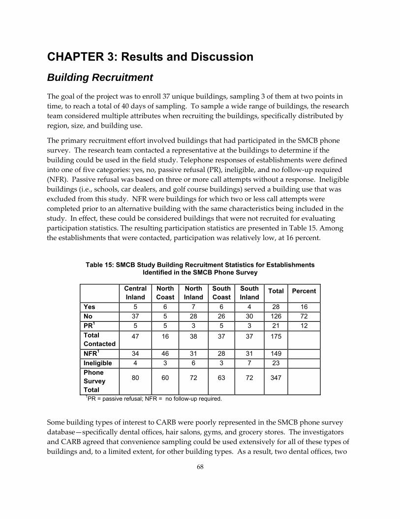
CHAPTER 3: Results and Discussion Building Recruitment The goal of the project was to enroll 37 unique buildings, sampling 3 of them at two points in time, to reach a total of 40 days of sampling.  To sample a wide range of buildings, the research team considered multiple attributes when recruiting the buildings, specifically distributed by region, size, and building use.   

The primary recruitment effort involved buildings that had participated in the SMCB phone survey.  The research team contacted a representative at the buildings to determine if the building could be used in the field study. Telephone responses of establishments were defined into one of five categories: yes, no, passive refusal (PR), ineligible, and no follow‐up required (NFR).  Passive refusal was based on three or more call attempts without a response.  Ineligible buildings (i.e., schools, car dealers, and golf course buildings) served a building use that was excluded from this study.  NFR were buildings for which two or less call attempts were completed prior to an alternative building with the same characteristics being included in the study.  In effect, these could be considered buildings that were not recruited for evaluating participation statistics. The resulting participation statistics are presented in Table 15. Among the establishments that were contacted, participation was relatively low, at 16 percent. 

Table 15: SMCB Study Building Recruitment Statistics for Establishments Identified in the SMCB Phone Survey

Central Inland

North Coast

North Inland

South Coast

South Inland

Total Percent

Yes 5 6 7 6 4 28 16 No 37 5 28 26 30 126 72 PR1 5 5 3 5 3 21 12 Total Contacted

47 16 38 37 37 175

NFR1 34 46 31 28 31 149 Ineligible 4 3 6 3 7 23 Phone Survey Total

80 60 72 63 72 347

1PR = passive refusal; NFR = no follow-up required.  

Some building types of interest to CARB were poorly represented in the SMCB phone survey database—specifically dental offices, hair salons, gyms, and grocery stores.  The investigators and CARB agreed that convenience sampling could be used extensively for all of these types of buildings and, to a limited extent, for other building types.  As a result, two dental offices, two 

68 

 

 

hair salons, one grocery store, one gym, and one restaurant were selected as convenience samples.   

The investigators selected the final two buildings via an Internet search.  The goal for the last two buildings was to increase the number of buildings in the Central Inland and South Inland regions, with a focus on retail stores or restaurants.  The investigators performed a Google search for retail stores, for Fresno, Kern, San Bernardino, Riverside, and Imperial Counties, and called establishments in order until two eligible and available buildings were found.  In total, the research team contacted 64 buildings during this process. 

Distribution of Buildings The goal was to recruit six buildings in each of five regions of the state, targeting the specific counties defined in the SMCB phone survey.  Below is a list of the regions, the targeted counties, and the unique number of buildings recruited in each county. Also noted are which regions included a repeated building.  The total number of buildings studied in the region is the sum of the number of buildings and the number of repeated buildings. 

• South Coast ‐ San Luis Obispo, San Diego Counties (7) 

• North Coast ‐ Alameda and Sonoma Counties (9) 

• South Inland ‐ Riverside, San Bernardino, and Imperial (7, 2 repeats) 

• Central Inland ‐ Fresno and Kern Counties (6, 1 repeat) 

• North Inland ‐ Placer and Solano Counties (8) 

 

Some of the buildings were outside the targeted counties, with the counties of all buildings noted in Table 16.  These were all recruited as a convenience sample to fill a particular building type that was difficult to recruit (e.g., hair salon, dental office). 

The next consideration was building size.  Ultimately, buildings were recruited from three size categories: Small (1000–12,000 ft2), Medium (12,000–25,000 ft2), and Medium/Large (25,000–50,000 ft2).  The goal was to recruit more small buildings, because a greater portion of the buildings in the state are small buildings.  Recruitment goals were met in all size categories.  Twenty‐four small buildings were included and repeat sampling was conducted on two of them, reaching the goal of 20 buildings.  Seven medium buildings were included and repeat sampling was conducted on one of them, reaching the goal of six buildings. Six Medium/Large buildings were included, reaching the goal of three in this size category. 

Finally, buildings with several different functions were included. The types of buildings and both the number included and the goal are listed below, along with the number of repeated buildings in each category: 

• Restaurants: 5 included, 1 repeated, goal of 4 buildings met 

• Retail: 7 included, goal of 6 buildings met  

69 

 

 

• Office: 8 included, 1 repeated, goal of 7 buildings met   

• Gym: 2 included, goal of  2 buildings met  

• Gas Station: 2 included, 1 repeated, goal of 2 buildings met  

• Beauty: 2 included, goal of 2 buildings met   

• Dental office: 2 included, goal of 2 buildings met   

• Healthcare: 2 included, goal of 2 buildings met   

• Grocery Store: 2 included, goal of 2 buildings met   

• Religious/Public Assembly: 2 included, goal of 2 buildings met   

• Other: 3 included, there were no goals in this category 

 

Building Descriptions A list of the buildings sampled, including the region, function, and size‐category, can be found in Table 16.  A description of each of the buildings is provided in Appendix B.  The descriptions are meant to provide a brief overview of the physical set‐up of the building and the types of sources and activities that occurred within the building.  These descriptions are meant to provide just a brief overview.   

A VOC summary for each building is included in Appendix B, indicating which compounds were found at higher levels compared to other buildings in the study.  Specifically, compounds whose concentrations fell in the top 25th percentile of the distribution of indoor concentrations are listed.  The actual concentrations are reported in the VOC section of this report.   

A brief summary of the PM concentrations is also provided in Appendix B.  Aspects such as where the samplers were located are included, particularly if there were significant differences in the measured indoor concentrations between the two samplers.  Potential indoor sources are discussed where applicable.   

A basic description of the HVAC system, as well some of the air exchange results, are provided in Appendix B. 

70 

 

 

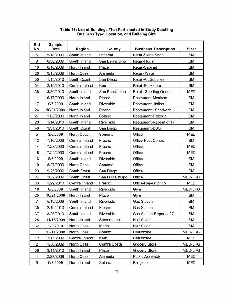
Table 16: List of Buildings That Participated in Study Detailing Business Type, Location, and Building Size

Bld No.

Sample Date Region County Business Description Size*

6 5/18/2009 South Inland Imperial Retail-Skate Shop SM 9 6/30/2009 South Inland San Bernardino Retail-Florist SM 10 6/16/2009 North Inland Placer Retail-Cabinet SM 20 9/15/2009 North Coast Alameda Retail- Water SM 30 1/15/2010 South Coast San Diego Retail-Art Supplies SM 34 2/18/2010 Central Inland Kern Retail-Bookstore SM 38 3/26/2010 South Inland San Bernardino Retail- Sporting Goods MED 11 6/17/2009 North Inland Placer Restaurant-Mexican SM 17 8/7/2009 South Inland Riverside Restaurant- Italian SM 26 10/21/2009 North Inland Placer Restaurant - Sandwich SM 27 11/3/2009 North Inland Solano Restaurant-Pizzeria SM 29 1/14/2010 South Inland Riverside Restaurant-Repeat of 17 SM 40 3/31/2010 South Coast San Diego Restaurant-BBQ SM 5 3/6/2009 North Coast Sonoma Office MED 13 7/16/2009 Central Inland Fresno Office-Pest Control SM 14 7/23/2009 Central Inland Fresno Office MED 15 7/24/2009 Central Inland Fresno Office MED 16 8/6/2009 South Inland Riverside Office SM 19 8/27/2009 North Coast Sonoma Office SM 23 9/25/2009 South Coast San Diego Office SM 24 10/2/2009 South Coast San Luis Obispo Office MED-LRG 33 1/29/2010 Central Inland Fresno Office-Repeat of 15 MED 18 8/8/2009 South Inland Riverside Gym MED-LRG 25 10/21/2009 North Inland Placer Gym SM 7 5/19/2009 South Inland Riverside Gas Station SM 35 2/19/2010 Central Inland Fresno Gas Station SM 37 3/25/2010 South Inland Riverside Gas Station-Repeat of 7 SM 28 11/13/2009 North Inland Sacramento Hair Salon SM 32 2/2/2010 North Coast Marin Hair Salon SM 1 12/11/2008 North Coast Solano Healthcare MED-LRG 12 7/15/2009 Central Inland Kern Healthcare MED 2 1/30/2009 North Coast Contra Costa Grocery Store MED-LRG 36 3/11/2010 North Inland Placer Grocery Store MED-LRG 4 2/27/2009 North Coast Alameda Public Assembly MED 8 6/2/2009 North Inland Solano Religious MED

71 

 

 

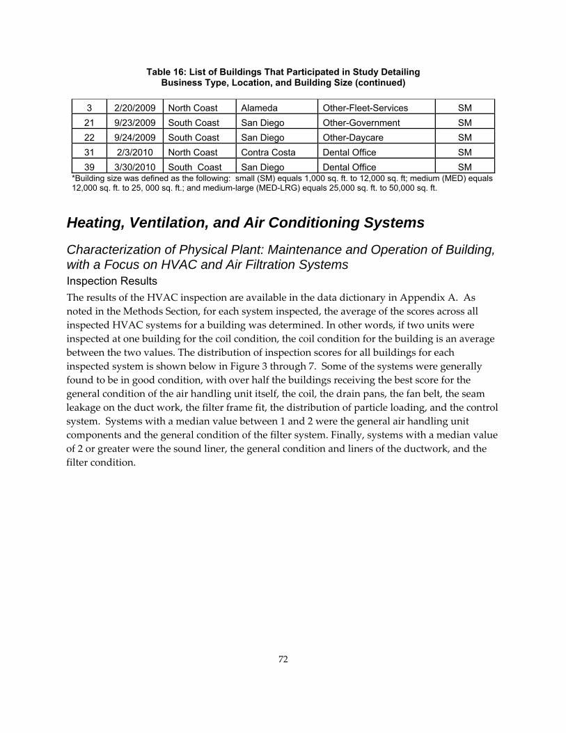
Table 16: List of Buildings That Participated in Study Detailing Business Type, Location, and Building Size (continued)

3 2/20/2009 North Coast Alameda Other-Fleet-Services SM 21 9/23/2009 South Coast San Diego Other-Government SM 22 9/24/2009 South Coast San Diego Other-Daycare SM 31 2/3/2010 North Coast Contra Costa Dental Office SM 39 3/30/2010 South Coast San Diego Dental Office SM

*Building size was defined as the following: small (SM) equals 1,000 sq. ft. to 12,000 sq. ft; medium (MED) equals 12,000 sq. ft. to 25, 000 sq. ft.; and medium-large (MED-LRG) equals 25,000 sq. ft. to 50,000 sq. ft.  

Heating, Ventilation, and Air Conditioning Systems

Characterization of Physical Plant: Maintenance and Operation of Building, with a Focus on HVAC and Air Filtration Systems Inspection Results The results of the HVAC inspection are available in the data dictionary in Appendix A.  As noted in the Methods Section, for each system inspected, the average of the scores across all inspected HVAC systems for a building was determined. In other words, if two units were inspected at one building for the coil condition, the coil condition for the building is an average between the two values. The distribution of inspection scores for all buildings for each inspected system is shown below in Figure 3 through 7.  Some of the systems were generally found to be in good condition, with over half the buildings receiving the best score for the general condition of the air handling unit itself, the coil, the drain pans, the fan belt, the seam leakage on the duct work, the filter frame fit, the distribution of particle loading, and the control system.  Systems with a median value between 1 and 2 were the general air handling unit components and the general condition of the filter system. Finally, systems with a median value of 2 or greater were the sound liner, the general condition and liners of the ductwork, and the filter condition. 

 

72 

 

 

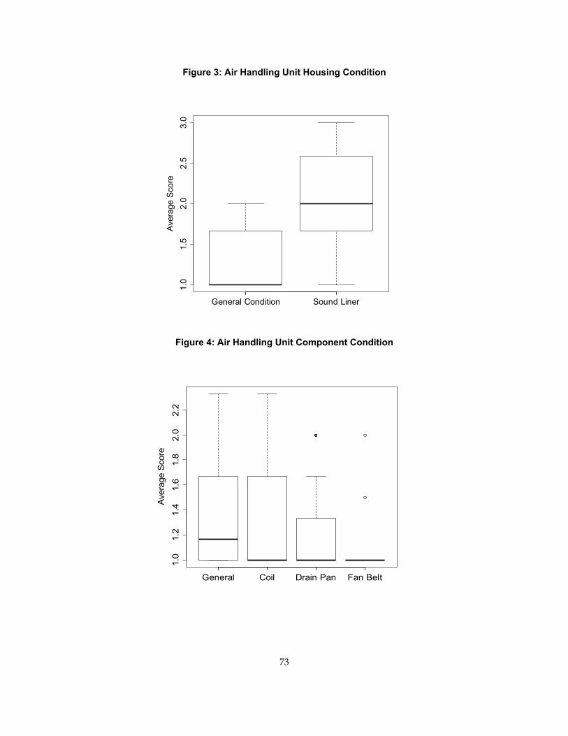
Figure 3: Air Handling Unit Housing Condition

1.0

1.5

2.0

2.5

3.0

Aver

age

Scor

e

General Condition Sound Liner

 

Figure 4: Air Handling Unit Component Condition

1.0

1.2

1.4

1.6

1.8

2.0

2.2

Aver

age

Scor

e

General Coil Drain Pan Fan Belt

 

73 

 

 

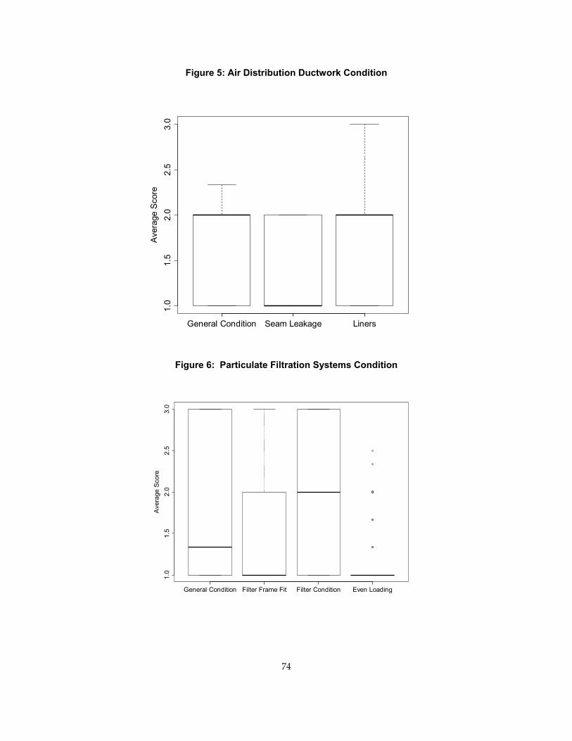
Figure 5: Air Distribution Ductwork Condition

1.0

1.5

2.0

2.5

3.0

Ave

rage

Sco

re

General Condition Seam Leakage Liners

 

Figure 6: Particulate Filtration Systems Condition 

1.0

1.5

2.0

2.5

3.0

Ave

rage

Sco

re

General Condition Filter Frame Fit Filter Condition Even Loading

 

74 

 

 

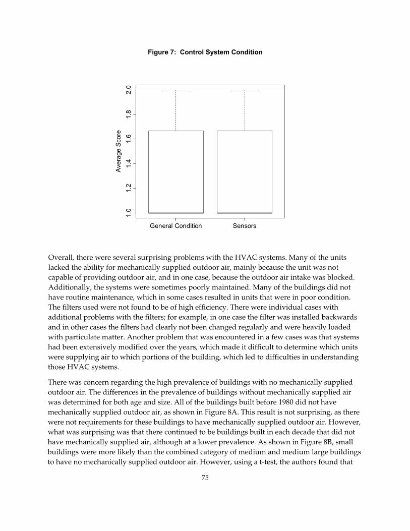
Figure 7: Control System Condition

1.0

1.2

1.4

1.6

1.8

2.0

Ave

rage

Sco

re

General Condition Sensors

 

Overall, there were several surprising problems with the HVAC systems. Many of the units lacked the ability for mechanically supplied outdoor air, mainly because the unit was not capable of providing outdoor air, and in one case, because the outdoor air intake was blocked. Additionally, the systems were sometimes poorly maintained. Many of the buildings did not have routine maintenance, which in some cases resulted in units that were in poor condition. The filters used were not found to be of high efficiency. There were individual cases with additional problems with the filters; for example, in one case the filter was installed backwards and in other cases the filters had clearly not been changed regularly and were heavily loaded with particulate matter. Another problem that was encountered in a few cases was that systems had been extensively modified over the years, which made it difficult to determine which units were supplying air to which portions of the building, which led to difficulties in understanding those HVAC systems. 

There was concern regarding the high prevalence of buildings with no mechanically supplied outdoor air. The differences in the prevalence of buildings without mechanically supplied air was determined for both age and size. All of the buildings built before 1980 did not have mechanically supplied outdoor air, as shown in Figure 8A. This result is not surprising, as there were not requirements for these buildings to have mechanically supplied outdoor air. However, what was surprising was that there continued to be buildings built in each decade that did not have mechanically supplied air, although at a lower prevalence. As shown in Figure 8B, small buildings were more likely than the combined category of medium and medium large buildings to have no mechanically supplied outdoor air. However, using a t‐test, the authors found that 

75 

 

 

the difference was not statistically significant. It is not surprising that the larger buildings had a higher prevalence of mechanically supplied outdoor air.  In the BASE study, which focused on large buildings, all of the buildings were able to supply outdoor air mechanically (Persily and Gorfain 2004).  In the study of small buildings completed in Florida, 43 of the 70 buildings evaluated did not have mechanically supplied outdoor air, which is a much greater fraction than found in this study (Cummings, Withers et al. 1996).  In part, this difference may be because the buildings in this study tended to be built more recently than the building in the Florida study.  Also, in the Florida study, air handlers were not consistently rooftop units, with only 19 buildings having rooftop units, while 5 buildings had air handlers outside, 13 buildings had air handlers in a mechanical room, 16 buildings had air handlers in mechanical closets (a space too small for a person to move around in), 4 buildings had air handlers in attics, 2 buildings had air handlers in ceilings, and 6 buildings had air handlers in an occupied space.  There were no other studies available to compare with this one to determine the prevalence of buildings without mechanically supplied outdoor air. 

 

76 

 

 

 

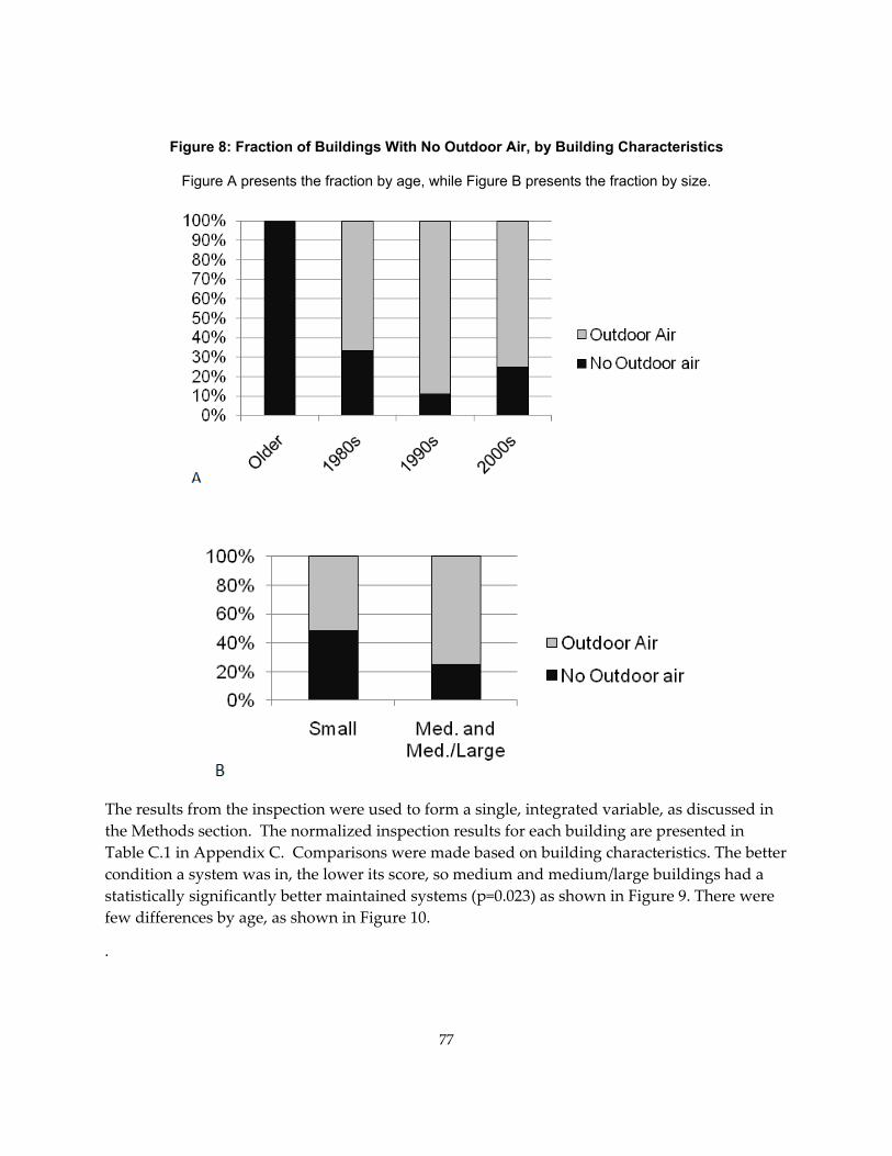
Figure 8: Fraction of Buildings With No Outdoor Air, by Building Characteristics

Figure A presents the fraction by age, while Figure B presents the fraction by size.

 

 

The results from the inspection were used to form a single, integrated variable, as discussed in the Methods section.  The normalized inspection results for each building are presented in Table C.1 in Appendix C.  Comparisons were made based on building characteristics. The better condition a system was in, the lower its score, so medium and medium/large buildings had a statistically significantly better maintained systems (p=0.023) as shown in Figure 9. There were few differences by age, as shown in Figure 10. 

. 

77 

 

 

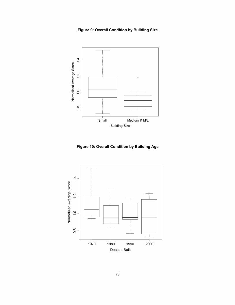
Figure 9: Overall Condition by Building Size

Small Medium & M/L

0.8

1.0

1.2

1.4

Building Size

Nor

mal

ized

Ave

rage

Sco

re

Figure 10: Overall Condition by Building Age 

1970 1980 1990 2000

0.8

1.0

1.2

1.4

Decade Built

Nor

mal

ized

Ave

rage

Sco

re

 

 

78 

 

 

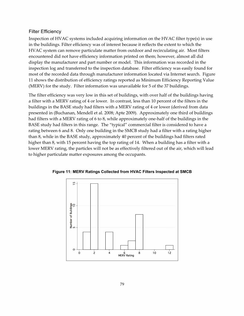
Filter Efficiency Inspection of HVAC systems included acquiring information on the HVAC filter type(s) in use in the buildings. Filter efficiency was of interest because it reflects the extent to which the HVAC system can remove particulate matter from outdoor and recirculating air.  Most filters encountered did not have efficiency information printed on them; however, almost all did display the manufacturer and part number or model.  This information was recorded in the inspection log and transferred to the inspection database.  Filter efficiency was easily found for most of the recorded data through manufacturer information located via Internet search.  Figure 11 shows the distribution of efficiency ratings reported as Minimum Efficiency Reporting Value (MERV) for the study.  Filter information was unavailable for 5 of the 37 buildings. 

The filter efficiency was very low in this set of buildings, with over half of the buildings having a filter with a MERV rating of 4 or lower.  In contrast, less than 10 percent of the filters in the buildings in the BASE study had filters with a MERV rating of 4 or lower (derived from data presented in (Buchanan, Mendell et al. 2008; Apte 2009).  Approximately one third of buildings had filters with a MERV rating of 6 to 8, while approximately one‐half of the buildings in the BASE study had filters in this range.  The “typical” commercial filter is considered to have a rating between 6 and 8.  Only one building in the SMCB study had a filter with a rating higher than 8, while in the BASE study, approximately 40 percent of the buildings had filters rated higher than 8, with 15 percent having the top rating of 14.  When a building has a filter with a lower MERV rating, the particles will not be as effectively filtered out of the air, which will lead to higher particulate matter exposures among the occupants. 

 

Figure 11: MERV Ratings Collected from HVAC Filters Inspected at SMCB

 

 

79 

 

 

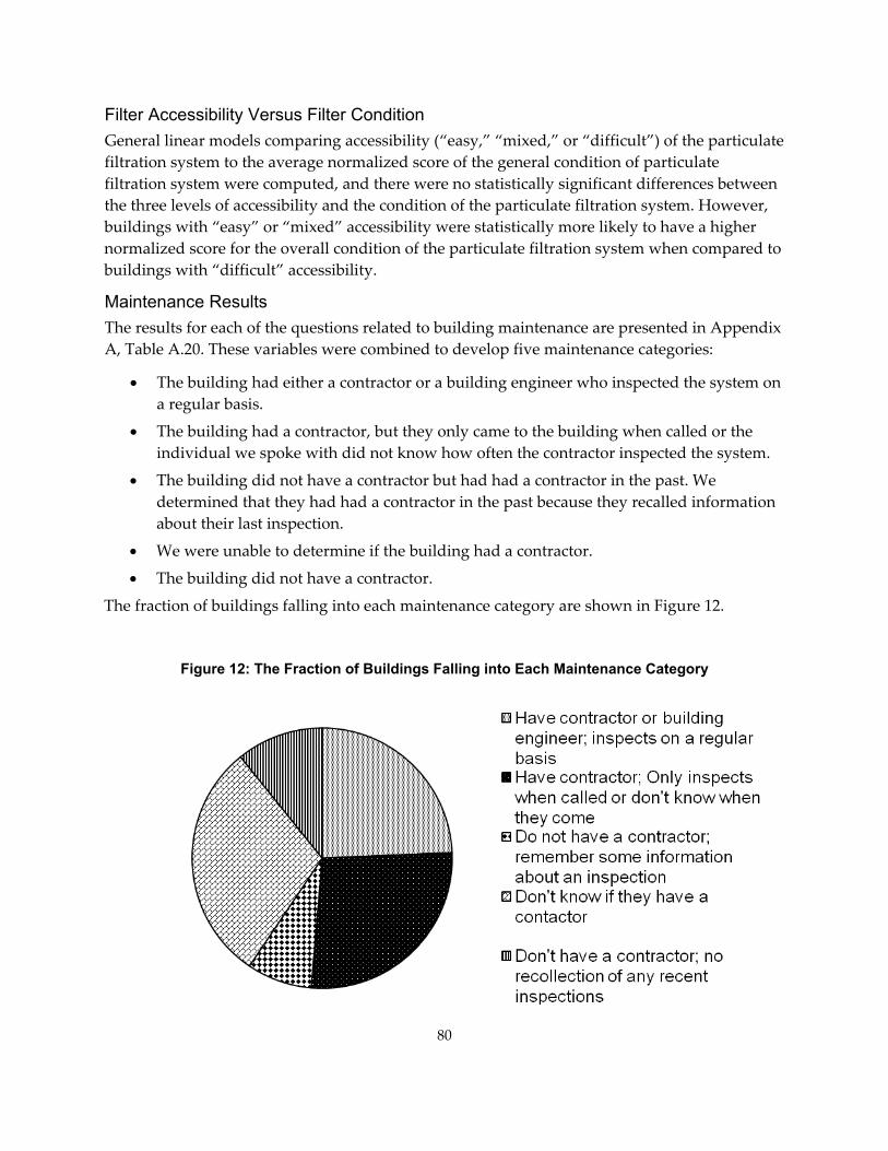
Filter Accessibility Versus Filter Condition General linear models comparing accessibility (“easy,” “mixed,” or “difficult”) of the particulate filtration system to the average normalized score of the general condition of particulate filtration system were computed, and there were no statistically significant differences between the three levels of accessibility and the condition of the particulate filtration system. However, buildings with “easy” or “mixed” accessibility were statistically more likely to have a higher normalized score for the overall condition of the particulate filtration system when compared to buildings with “difficult” accessibility.  

Maintenance Results The results for each of the questions related to building maintenance are presented in Appendix A, Table A.20. These variables were combined to develop five maintenance categories: 

• The building had either a contractor or a building engineer who inspected the system on a regular basis. 

• The building had a contractor, but they only came to the building when called or the individual we spoke with did not know how often the contractor inspected the system. 

• The building did not have a contractor but had had a contractor in the past. We determined that they had had a contractor in the past because they recalled information about their last inspection. 

• We were unable to determine if the building had a contractor. 

• The building did not have a contractor. 

The fraction of buildings falling into each maintenance category are shown in Figure 12. 

 

Figure 12: The Fraction of Buildings Falling into Each Maintenance Category 

 80 

 

 

 

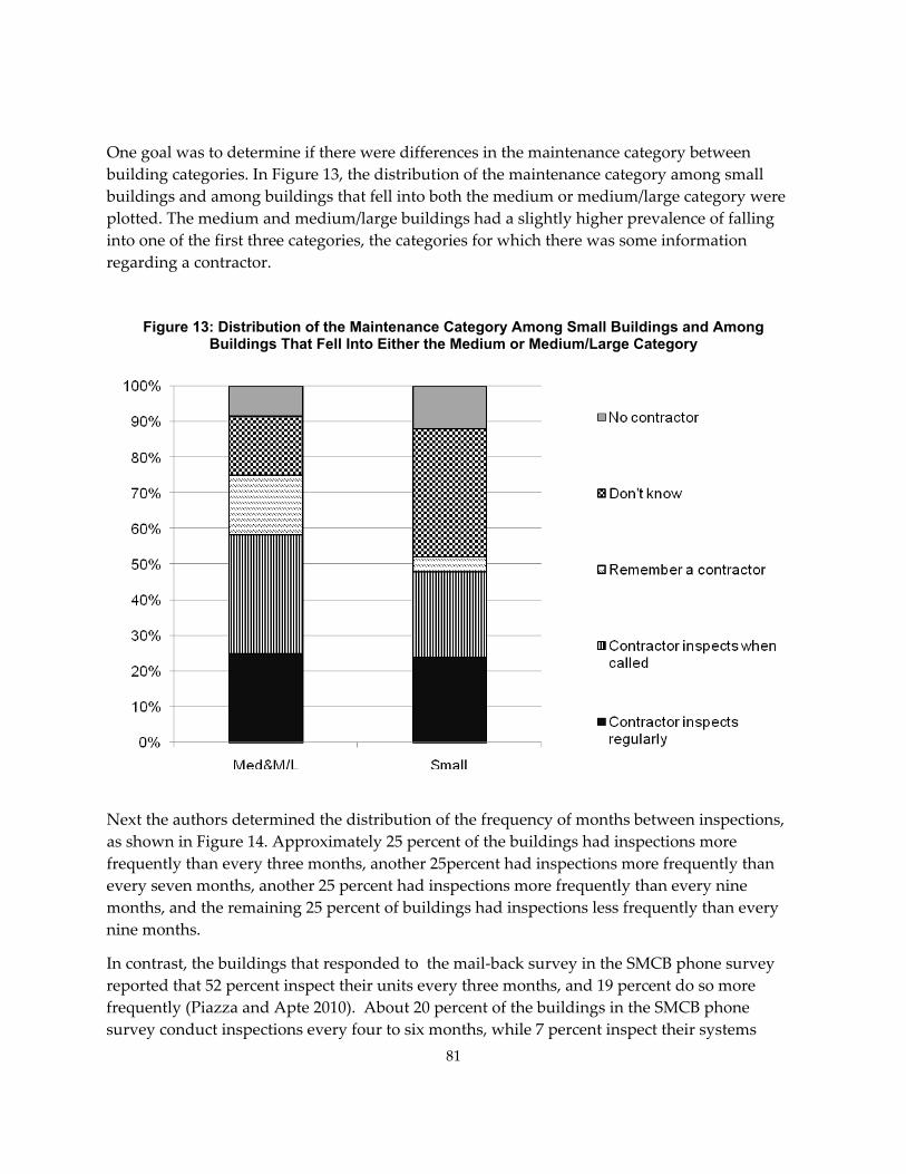
One goal was to determine if there were differences in the maintenance category between building categories. In Figure 13, the distribution of the maintenance category among small buildings and among buildings that fell into both the medium or medium/large category were plotted. The medium and medium/large buildings had a slightly higher prevalence of falling into one of the first three categories, the categories for which there was some information regarding a contractor. 

 

Figure 13: Distribution of the Maintenance Category Among Small Buildings and Among Buildings That Fell Into Either the Medium or Medium/Large Category

Next the authors determined the distribution of the frequency of months between inspections, as shown in Figure 14. Approximately 25 percent of the buildings had inspections more frequently than every three months, another 25percent had inspections more frequently than every seven months, another 25 percent had inspections more frequently than every nine months, and the remaining 25 percent of buildings had inspections less frequently than every nine months.   

In contrast, the buildings that responded to  the mail‐back survey in the SMCB phone survey reported that 52 percent inspect their units every three months, and 19 percent do so more frequently (Piazza and Apte 2010).  About 20 percent of the buildings in the SMCB phone survey conduct inspections every four to six months, while 7 percent inspect their systems 

81 

 

 

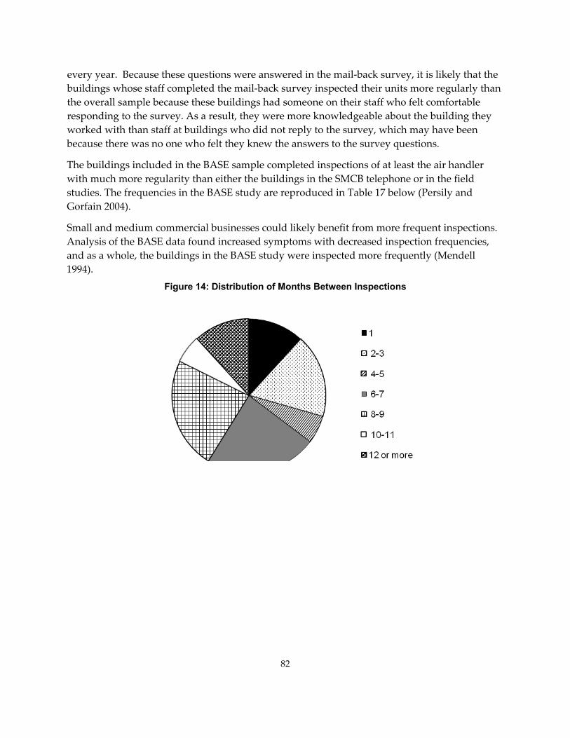
every year.  Because these questions were answered in the mail‐back survey, it is likely that the buildings whose staff completed the mail‐back survey inspected their units more regularly than the overall sample because these buildings had someone on their staff who felt comfortable responding to the survey. As a result, they were more knowledgeable about the building they worked with than staff at buildings who did not reply to the survey, which may have been because there was no one who felt they knew the answers to the survey questions.   

The buildings included in the BASE sample completed inspections of at least the air handler with much more regularity than either the buildings in the SMCB telephone or in the field studies. The frequencies in the BASE study are reproduced in Table 17 below (Persily and Gorfain 2004).  

Small and medium commercial businesses could likely benefit from more frequent inspections.  Analysis of the BASE data found increased symptoms with decreased inspection frequencies, and as a whole, the buildings in the BASE study were inspected more frequently (Mendell 1994). 

Figure 14: Distribution of Months Between Inspections

 

 

82 

 

 

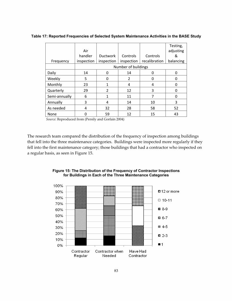
Table 17: Reported Frequencies of Selected System Maintenance Activities in the BASE Study

Frequency 

Air handler 

inspectionDuctwork inspection

Controls inspection

Controls recalibration 

Testing, adjusting 

& balancing 

   Number of buildings Daily  14  0  14  0  0 Weekly  5  0  2  0  0 Monthly  23  1  4  4  0 Quarterly  29  2  12  3  0 Semi‐annually  6  1  11  7  0 Annually  3  4  14  10  3 As needed  4  32  28  58  52 None  0  59  12  15  43 Source: Reproduced from (Persily and Gorfain 2004) 

 

The research team compared the distribution of the frequency of inspection among buildings that fell into the three maintenance categories.  Buildings were inspected more regularly if they fell into the first maintenance category; those buildings that had a contractor who inspected on a regular basis, as seen in Figure 15. 

Figure 15: The Distribution of the Frequency of Contractor Inspections for Buildings in Each of the Three Maintenance Categories

83 

 

 

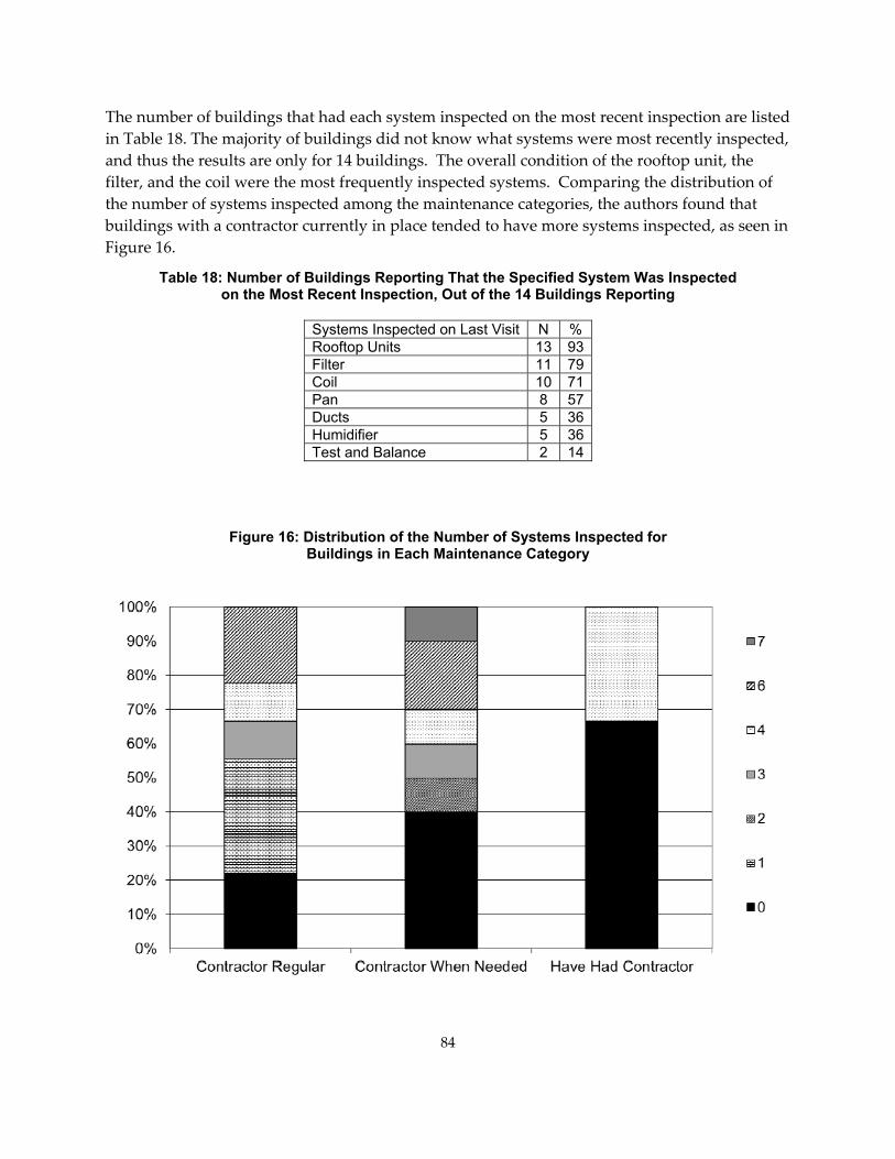
The number of buildings that had each system inspected on the most recent inspection are listed in Table 18. The majority of buildings did not know what systems were most recently inspected, and thus the results are only for 14 buildings.  The overall condition of the rooftop unit, the filter, and the coil were the most frequently inspected systems.  Comparing the distribution of the number of systems inspected among the maintenance categories, the authors found that buildings with a contractor currently in place tended to have more systems inspected, as seen in Figure 16. 

Table 18: Number of Buildings Reporting That the Specified System Was Inspected on the Most Recent Inspection, Out of the 14 Buildings Reporting

Systems Inspected on Last Visit N % Rooftop Units 13 93Filter 11 79Coil 10 71Pan 8 57Ducts 5 36Humidifier 5 36Test and Balance 2 14

 

 

Figure 16: Distribution of the Number of Systems Inspected for Buildings in Each Maintenance Category

84 

 

 

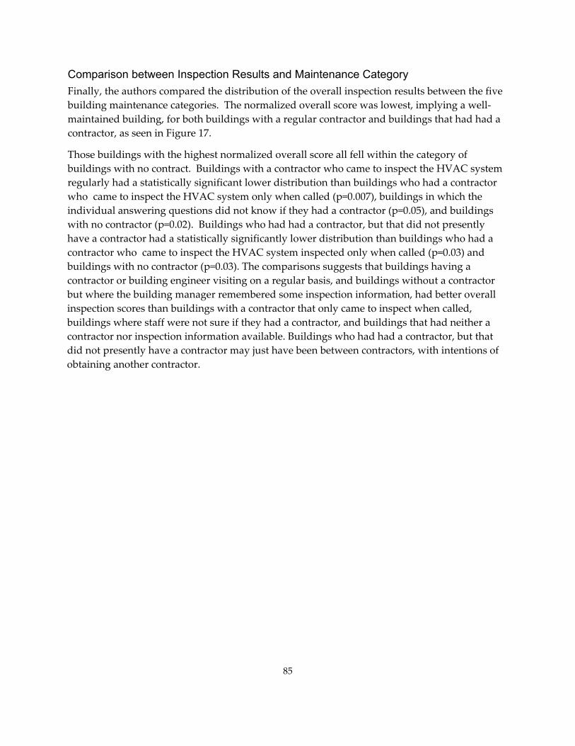
Comparison between Inspection Results and Maintenance Category Finally, the authors compared the distribution of the overall inspection results between the five building maintenance categories.  The normalized overall score was lowest, implying a well‐maintained building, for both buildings with a regular contractor and buildings that had had a contractor, as seen in Figure 17.  

Those buildings with the highest normalized overall score all fell within the category of buildings with no contract.  Buildings with a contractor who came to inspect the HVAC system regularly had a statistically significant lower distribution than buildings who had a contractor who  came to inspect the HVAC system only when called (p=0.007), buildings in which the individual answering questions did not know if they had a contractor (p=0.05), and buildings with no contractor (p=0.02).  Buildings who had had a contractor, but that did not presently have a contractor had a statistically significantly lower distribution than buildings who had a contractor who  came to inspect the HVAC system inspected only when called (p=0.03) and buildings with no contractor (p=0.03). The comparisons suggests that buildings having a contractor or building engineer visiting on a regular basis, and buildings without a contractor but where the building manager remembered some inspection information, had better overall inspection scores than buildings with a contractor that only came to inspect when called, buildings where staff were not sure if they had a contractor, and buildings that had neither a contractor nor inspection information available. Buildings who had had a contractor, but that did not presently have a contractor may just have been between contractors, with intentions of obtaining another contractor.  

85 

 

 

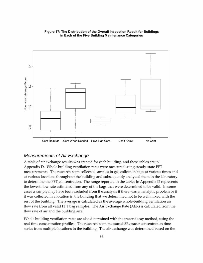
Figure 17: The Distribution of the Overall Inspection Result for Buildings in Each of the Five Building Maintenance Categories 

Cont Regular Cont When Needed Have Had Cont Don't Know No Cont

0.8

1.0

1.2

1.4

Nor

mal

ized

Ave

rage

Sco

re

Measurements of Air Exchange A table of air exchange results was created for each building, and these tables are in Appendix D.  Whole building ventilation rates were measured using steady‐state PFT measurements.  The research team collected samples in gas collection bags at various times and at various locations throughout the building and subsequently analyzed them in the laboratory to determine the PFT concentration.  The range reported in the tables in Appendix D represents the lowest flow rate estimated from any of the bags that were determined to be valid.  In some cases a sample may have been excluded from the analysis if there was an analytic problem or if it was collected in a location in the building that we determined not to be well mixed with the rest of the building.  The average is calculated as the average whole‐building ventilation air flow rate from all valid PFT bag samples.  The Air Exchange Rate (AER) is calculated from the flow rate of air and the building size. 

Whole building ventilation rates are also determined with the tracer decay method, using the real‐time concentration profiles.  The research team measured SF6 tracer concentration time series from multiple locations in the building.  The air exchange was determined based on the 

86 

 

 

natural logarithm of measured tracer decay versus time for each location in the building.  In some cases there may have been changes in the slope of the decay over time, and scientific judgment was used to select the most appropriate time period.  The smallest and largest measured AER values are listed as the range reported in the tables in Appendix D. The tabulated average is the mean air exchange calculated at all the sampling locations in the building.  The ventilation air flow rate was calculated from the product of the AER and the building volume. 

Whole building ventilation rates were also determined with the tracer decay method, using concentrations collected at distinct time points during the decay period.  Samples were collected from multiple locations within the building. The decay slope was calculated from the natural logarithm of tracer concentration of the samples versus time at any one location to determine the AER.  The smallest and largest values calculated are listed as the range reported in the tables in Appendix D.  The average is the average between all calculated values.  Once again, the ventilation air flow rate was calculated from the product of the AER and the building volume.  As both this method and the concentration from the real‐time concentration profiles are based on the natural logarithm of the slope of the concentration of SF6 versus time, it is expected that they would have comparable results.  Differences may occur if the samplers were not co‐located and there was significant variation in the time‐profile of the concentrations in various locations in the building.  Also, differences may arise if there was variability in the slope over time, potentially due to variability in the air exchange rate over time, and the time period captured by the point samples did not cover the same span as represented by the continuous concentration. Expert judgment was used to determine the differences. 

Whole building ventilation rates were also estimated using the CO2 equilibrium method.  The authors generated plots of the continuous CO2 concentrations (using a 10‐minute averaging period) and inspected the plots visually to determine if an equilibrium value was obtained.  In some cases, two time periods were selected that both appeared to have the indoor minus outdoor CO2 concentration at equilibrium.  Using the difference between the indoor and outdoor CO2 concentration at a given location, along with the number of building occupants and the CO2 generation rate appropriate for the building level, a whole‐building ventilation air flow rate was determined.  In most cases, the research team used the CO2 generation rate associated with a sedentary office worker, specifically 0.31 L/min.  If a different value was used, it is noted as a footnote in the tables in Appendix D.  The range reported in those tables represents the minimum and maximum value calculated, either if there were multiple locations where CO2 concentrations were measured in the building or if air flow rates were determined from concentrations at different time points.  If there was only one CO2 monitor in the building, and steady state was only obtained at one point in time, no values are listed in the range, as only one value was calculated.  The tabulated average is the mean of these values.  The AER is calculated from the product of the ventilation air flow rate and the building volume.  In some buildings a CO2 equilibrium concentration was not reached, in which case no values are listed.  

The total mechanically supplied air as measured by the TRAMS method was also measured.  For each air handling unit, anywhere from one to three TRAMS runs was conducted.  If the 

87 

 

 

building had multiple air handling units, TRAMS runs were completed on as many air handling units as was feasible.  If there was only one air handling unit (AHU), the tabulated range reported in the tables in Appendix D represents the range of supply air flow calculated from each TRAMS run, with the tabulated average being the mean of these values.  If there were multiple AHUs, the tabulated average was calculated for each unit, with the supply air flow from the unit with the lowest rate listed as the lower end of the range and the rate from the unit with the largest air flow listed as the higher end of the range.  The average supply air flow rate of each unit was then summed.  If TRAMS runs were conducted on all of the AHUs for the space, this sum is the calculated whole‐building supply air flow.  If not all AHUs received TRAMS measurements, a footnote is included to inform the reader of the number of AHUs at the building, and the number of units measured.  If the CO2 was injected into the return grille and there was outside air supplied to the HVAC unit, it is noted in a footnote, as this results in an underestimation.   

 The total mechanically supplied air at the supply vents using a balometer was measured in some of the buildings.  In cases where this method was used, all supply vents were measured and the airflow was summed.  In many cases the research team was also able to measure flow through both the return ducts and supply ducts.  The mechanically supplied outdoor air was measured, in most cases, using a Duct Blaster, generally with one Duct Blaster run completed for each air handling unit.  The team made Duct Blaster measurements on as many AHUs as feasible, and the results were summed.  In a limited number of buildings, the research team was unable to use the Duct Blaster and used a calibrated blower door or a Balometer instead.  The fraction outdoor air in the supply flow was determined generally using measurements of CO2.  In one pilot building, the research team used SF6.  The average fraction of outside air from measurements at multiple vents was calculated. 

Completion of Ventilation Measurements The research team used multiple measurement methods to characterize building ventilation rate. Not all measurement methods are feasible on all buildings. To measure the whole‐building ventilation rate, the Steady State Air Exchange Method and the Tracer Decay Method was employed in all buildings. The CO2 Equilibrium Method was applicable only in buildings with a stable occupancy pattern, and valid measures were obtained in 33 buildings.  

Mechanical ventilation supply was measured in two parts: the total volume of mechanically supplied air, and the volume of mechanically supplied outdoor air.  Total volume of mechanically supplied air was measured using TRAMS, with 17 buildings having TRAMS measurements conducted on all of the HVAC unit and 11 buildings having TRAMS measurements conducted only on a portion of the HVAC units. TRAMS measurements could not be made in 12 buildings, generally because the supply vents were not accessible or because the supply vents did not contain a long enough section for mixing. Supply Register measurements using a balometer were completed in 11 buildings.  

In addition, the research team was able to determine the percent of outdoor air in 19 of 25 buildings by measuring the CO2 concentrations in the supply ducts, in the interior of the 

88 

 

 

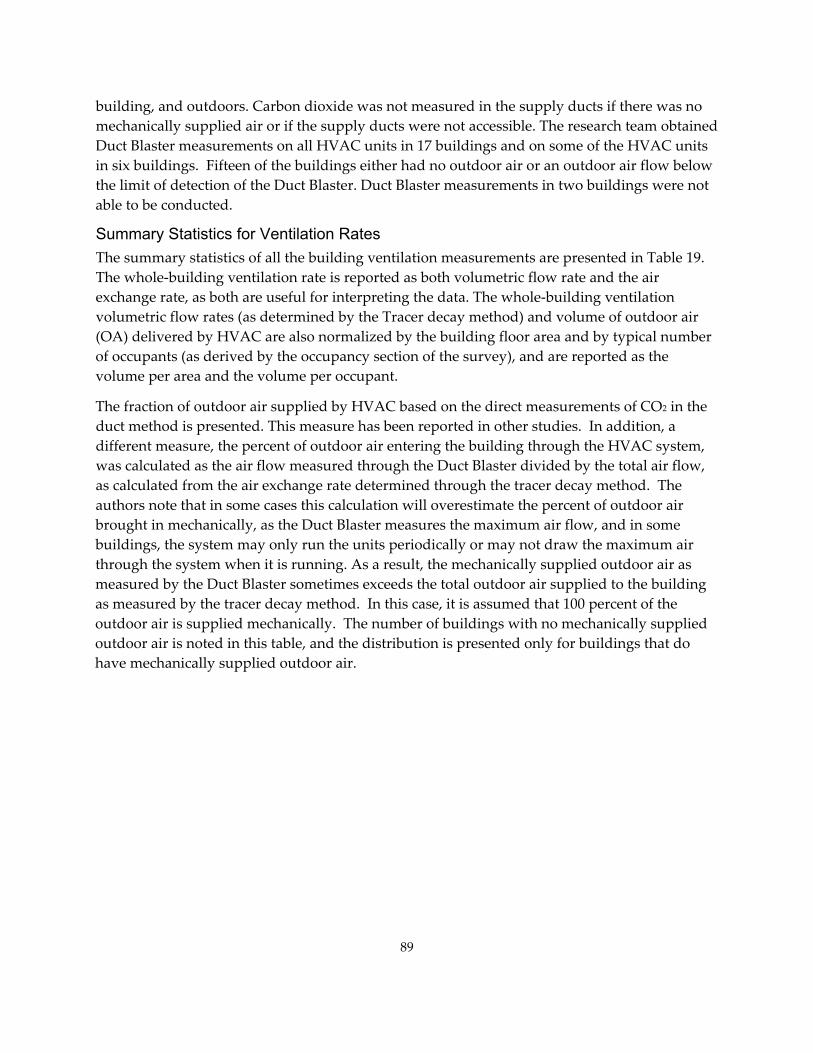
89 

 

building, and outdoors. Carbon dioxide was not measured in the supply ducts if there was no mechanically supplied air or if the supply ducts were not accessible. The research team obtained Duct Blaster measurements on all HVAC units in 17 buildings and on some of the HVAC units in six buildings.  Fifteen of the buildings either had no outdoor air or an outdoor air flow below the limit of detection of the Duct Blaster. Duct Blaster measurements in two buildings were not able to be conducted. 

Summary Statistics for Ventilation Rates The summary statistics of all the building ventilation measurements are presented in Table 19. The whole‐building ventilation rate is reported as both volumetric flow rate and the air exchange rate, as both are useful for interpreting the data. The whole‐building ventilation volumetric flow rates (as determined by the Tracer decay method) and volume of outdoor air (OA) delivered by HVAC are also normalized by the building floor area and by typical number of occupants (as derived by the occupancy section of the survey), and are reported as the volume per area and the volume per occupant.  

The fraction of outdoor air supplied by HVAC based on the direct measurements of CO2 in the duct method is presented. This measure has been reported in other studies.  In addition, a different measure, the percent of outdoor air entering the building through the HVAC system, was calculated as the air flow measured through the Duct Blaster divided by the total air flow, as calculated from the air exchange rate determined through the tracer decay method.  The authors note that in some cases this calculation will overestimate the percent of outdoor air brought in mechanically, as the Duct Blaster measures the maximum air flow, and in some buildings, the system may only run the units periodically or may not draw the maximum air through the system when it is running. As a result, the mechanically supplied outdoor air as measured by the Duct Blaster sometimes exceeds the total outdoor air supplied to the building as measured by the tracer decay method.  In this case, it is assumed that 100 percent of the outdoor air is supplied mechanically.  The number of buildings with no mechanically supplied outdoor air is noted in this table, and the distribution is presented only for buildings that do have mechanically supplied outdoor air. 

 

 

 

 

Table 19: Distribution of Building Ventilation Rate 

Label Na Mean SD Min 25th Pctl Median 75th

Pctl 95th Pctl Max

Whole-building ventilation rate Whole-building ventilation rate measured by Steady State Air Exchange Method (cfm) 40 1,245 2,220 44 202 561 1,317 5,077 12,434

Whole-building ventilation rate by Tracer Decay Method (cfm) 40 1,585 1,951 87 305 980 1,878 5,233 10,291Whole-building ventilation rate per area, Tracer Decay Method (cfm/ft2) 40 0.27 0.27 0.02 0.12 0.19 0.3 0.77 1.51

Whole-building ventilation rate per person, Tracer Decay Method (cfm/person) 40 130 151 14 36 76 152 553 680

Air exchange rate measured by Steady-State Air Exchange Method (PFT) (h-1) 40 1.03 1.08 0.12 0.43 0.73 1.23 2.54 6.26

Air exchange rate measured by Tracer Decay Method (SF6) (h-1) 40 1.62 1.65 0.3 0.71 1.04 1.89 4.67 9.07Total mechanical ventilation supply Mechanic. supplied ventilation by supply vent (cfm) 11 3,625 6,103 664 940 1,561 2,463 21,435 21,435Mechanic. supplied ventilation by TRAMSb (cfm) 17 4,611 7,493 700 2,163 2,831 3,863 33,360 33,360Mechanic. supplied ventilation per area by TRAMSb (cfm/ft2) 17 1.32 0.70 0.34 0.86 1.11 1.77 2.64 2.64Outdoor air mechanically supply Outdoor air deliver rate by HVAC by Duct Blaster (cfm) 22 2,188 2,972 110 512 1,162 2,486 6,716 12,646Outdoor air deliver rate by HVAC per area (cfm/ft2) 40 0.13 0.23 0 0 0.04 0.15 0.66 1.07Outdoor air deliver rate by HVAC per person (cfm/person) 40 48 66 0 0 13 74 188 220Fraction of outdoor air supplied by HVAC to building Calculated based on Duct Blaster and Tracer Decay methodc (%) 14 45 26 10 17 47 68 82 82Fraction of outdoor air in HVAC supply air Direct measurements by the CO2 Ratio Method (%) 20 23 17 0 12 19 32 57 64

Note: a Note all measurements were feasible in all buildings. b Only those buildings with full TRAMS were included. c 16 buildings has no mechanically supplied outdoor air and 9 buildings had 100% of mechanically supplied outdoor air. Only the distribution of values between 0 and 1 were presented. SD = Standard Deviation

90 

 

 

Comparison of Methods for Determining Whole Building Ventilation Rates Box plots of the distributions of the whole‐building ventilation rates are presented in Figure 18. The CO2 equilibrium was determined to be unreliable, as in some cases CO2 concentrations never reached steady state. Also, in some cases, building occupancies were often not all that consistent, making results unreliable.  In addition, if building occupancy was low, the difference between the indoor and outdoor concentrations of CO2 was small, and therefore due to uncertainties in absolute concentration, there was uncertainty in the difference in CO2 concentrations. The distribution of air exchange rates as calculated by the PFT steady‐state method was lower than as calculated by the SF6 decay method. 

The correlation between each of the air exchange methods was calculated.  The R2 value for the correlation between the SF6 decay method and the PFT method was 0.76, between the PFT and CO2 equilibrium was 0.84, and between the SF6 and the CO2 equilibrium was 0.74. 

The authors compared the air exchange rate calculated using the steady‐state method for each building to the value calculated using the tracer decay method in the scatter plot presented in Figure 19.  The one‐to‐one line is also plotted in the figure.  It is clear that the air exchange rates as measured using the steady‐state method tended to be lower than those using the tracer decay method.  There are two likely reasons for this.  The primary reason is that the steady‐state measure is influenced by the nighttime period, which likely has a lower air exchange rate because the building is not occupied, thereby limiting doors being open and closed and likely reducing the amount of mechanically drawn air being introduced.  The second reason is that in a limited number of cases, there may not have been as complete mixing of the tracer initially, which may have resulted in a higher air exchange rate, as the tracer was primarily in regions of the building that had significant air flow.  It is thought that the differences primarily result from the influence of the nighttime period, and as the goal of the project was primarily to determine the air exchange rate during the occupied period, the results calculated from the tracer decay method were used as the primary air exchange measure. 

The BASE study determined that air exchange measurements calculated using CO2 measurements were the most robust (Persily and Gorfain 2004).  However, the study spaces in the BASE study were quite different; all were densely occupied office spaces, which would improve the validity of air exchange rates calculated by the CO2 method.  In SMCBs of varied uses, which tend to have lower occupant density than those in the BASE study, the researchers found that the CO2 method did not work in many cases, as the CO2 concentration never came to equilibrium.  The tracer gas was able to be mixed through the whole building in these smaller buildings.  Therefore, the authors of this report recommend the tracer decay method for future studies of air exchange in SMCB of varied uses. 

It is further noted that there was usually good agreement between the total flow rate measured from the supply grilles and the return grilles. 

 

91 

 

 

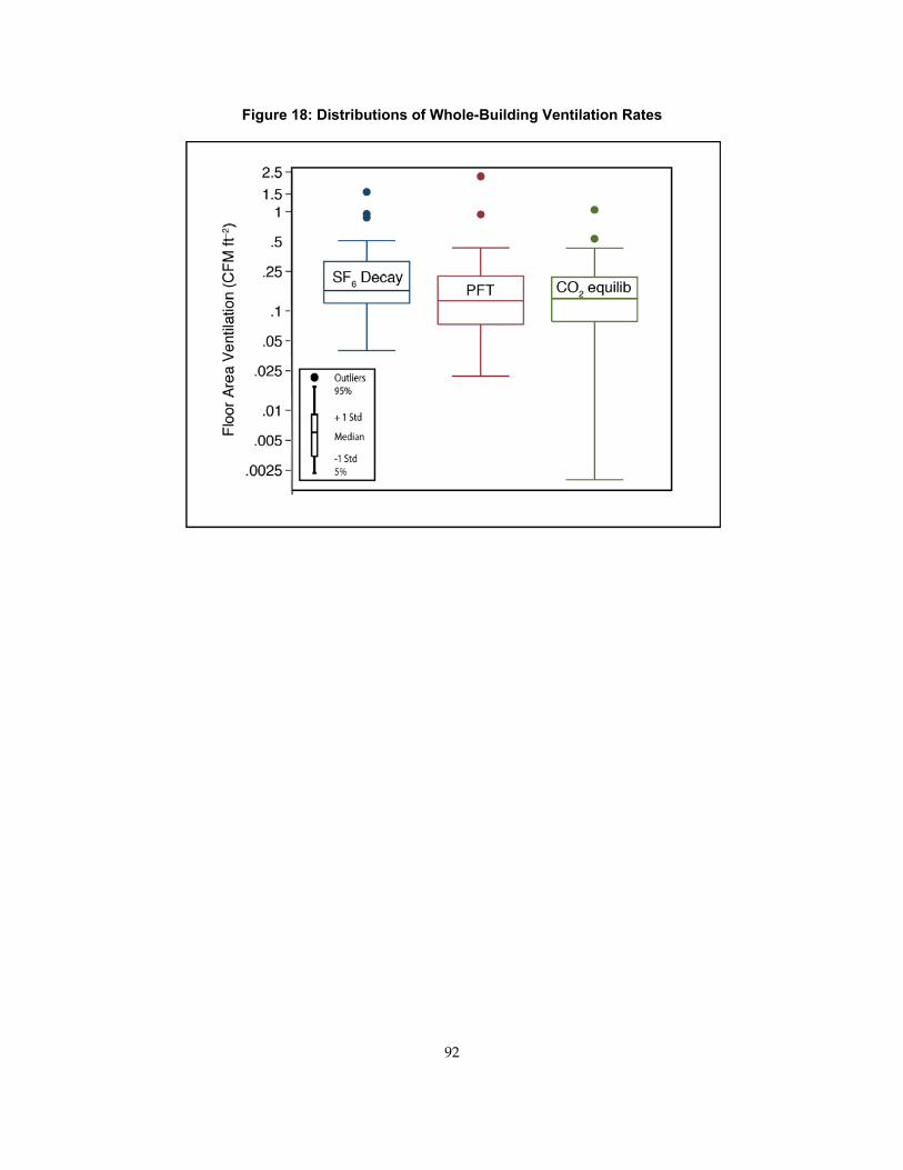
Figure 18: Distributions of Whole-Building Ventilation Rates

 

  

92 

 

 

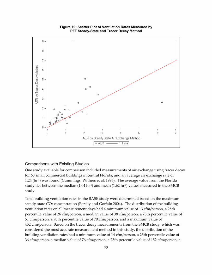
Figure 19: Scatter Plot of Ventilation Rates Measured by PFT Steady-State and Tracer Decay Method

 

 

Comparisons with Existing Studies One study available for comparison included measurements of air exchange using tracer decay for 68 small commercial buildings in central Florida, and an average air exchange rate of 1.24 (hr‐1) was found (Cummings, Withers et al. 1996).  The average value from the Florida study lies between the median (1.04 hr‐1) and mean (1.62 hr‐1) values measured in the SMCB study.   

Total building ventilation rates in the BASE study were determined based on the maximum steady‐state CO2 concentration (Persily and Gorfain 2004).  The distribution of the building ventilation rates on all measurement days had a minimum value of 13 cfm/person, a 25th percentile value of 26 cfm/person, a median value of 38 cfm/person, a 75th percentile value of 51 cfm/person, a 90th percentile value of 70 cfm/person, and a maximum value of 452 cfm/person.  Based on the tracer decay measurements from the SMCB study, which was considered the most accurate measurement method in this study, the distribution of the building ventilation rates had a minimum value of 14 cfm/person, a 25th percentile value of 36 cfm/person, a median value of 76 cfm/person, a 75th percentile value of 152 cfm/person, a 

93 

 

 

95th percentile value of 553 cfm/person, and a maximum value of 680 cfm/person.  The air exchange rates measured in this study on a per‐person basis were considerably higher than those measured in the BASE study. 

Outdoor mechanically supplied measurements were made in a portion of the classrooms studied in the portable classroom study.  In portable classrooms, the mean value was 0.95 cfm/ft2, while in traditional classrooms the mean was 0.80 cfm/ft2.  This value was much higher than the mean value of mechanically supplied air we measured (0.13 cfm/ft2) and even much higher than the total outdoor air delivered (0.27 cfm/ft2).  As with the BASE study, classrooms are densely occupied, and this may be in part the reason for the significantly higher values. 

Finally, the authors compare the air exchange rates measured in this study to those measured in new homes in California.  In a sample of 108 new single‐family homes, air exchange measurements were made using the steady‐state PFT technique also used in this study (Offermann 2009).  The minimum air exchange rate was 0.09 (hr‐1), the median was 0.26 (hr‐1), and the maximum was 5.3 (hr‐1)—much lower than the values measured in this study.  The minimum value in this study was 0.3 (hr‐1), which is greater than the median in new homes.  It is important to note that new homes in California have much lower air exchange rates than older homes, with the distribution of a random sample of southern California and Arizona homes measured primarily in the 1980s having an arithmetic mean of 1.81 (hr‐1) and a geometric mean of 0.61 (hr‐1) (Pandian, Behar et al. 1998).  It is expected that commercial buildings would have higher air exchange rates than homes because more outdoor air is needed to supply a higher occupancy density. 

The total mechanically supplied air flow can both be compared to the typical design standard,  nominally 1 cfm/ft2, and to the values measured in the BASE study (Persily and Gorfain 2004).  The buildings in the BASE study had a mean value of 1.04 cfm/ft2, a minimum value of 0.17 cfm/ft2, a 25th percentile value of 0.61 cfm/ft2, a median value of 0.94 cfm/ft2, a 75th percentile value of 1.24 cfm/ft2, a 90th percentile value of 1.73 cfm/ft2, and a maximum value of 4.15 cfm/ft2.  In comparison, the buildings in this  study had a mean value of 1.32 cfm/ft2, a minimum value of 0.34 cfm/ft2, a 25th percentile value of 0.86 cfm/ft2, a median value of 1.11 cfm/ft2, a 75th percentile value of 1.77 cfm/ft2, a 95th percentile value of 2.64 cfm/ft2, and a maximum of 2.64 cfm/ft2, indicating that the flow rates in the SMCB buildings in this study had slightly higher supply flow rates than those in the BASE study.  Additionally, it is noted that in some cases the value reported in this study underestimates the air flow, which would further increase the flow rates relative to the BASE study. A significant portion of the buildings in this study had supply flow rates significantly higher than the nominal design standard. 

The fraction of outdoor air in the supply vent as measured by the CO2 ratio can also be compared to the values measured in the BASE study.  The distribution of the outdoor air in the supply vent on all measurement days as measured by the CO2 ratio had a minimum value of 0, a 10th percentile value of 0.03, a 25th percentile value of 0.11, a median value of 0.23, a 75th percentile value of 0.44, a 90th percentile value of 0.75, and a maximum of 1.2.  It is noted that 

94 

 

 

the minimum value is 0; however, the text indicates that some buildings were capable of providing mechanically supplied outdoor air but were set not to provide any outdoor air.  Comparing just to the distribution of the buildings in this study that were capable of supplying outdoor air, with a minimum value of 0, a 25th percentile value of 0.12, a median value of 0.19, a 75th percentile value of 0.32, a 95th percentile value of 0.57, and a maximum of 0.64, this study had a much narrower range of values with a slightly lower median value.   

Factors Influencing Air Exchange Rate One of the objectives was to determine factors that influenced the distribution of air exchange rates. The authors made comparisons of air exchange rates by age, location, size, and use. 

Building age: No statistically significant difference in the whole‐building ventilation rate was found by any of the three age split criteria: 1983, 1990, and 2000 (Figure 20). By looking at the scatter plot of air exchange rate versus the year when building was built, there is no obvious linear relationship between air exchange rate and building age. 

Building region: Analysis of variance found no statistically significant difference in the whole‐building ventilation rate among the five regions studied (Figure 21).  Further comparison between the northern‐coastal region (which was cooler than other regions) and the other four regions combined also resulted in no statistically significant difference. 

Building size: The whole‐building ventilation rates per area and per person were not significantly different among the small, medium, and medium/large buildings (Figure 22). The medium and medium/large buildings were combined and compared with small buildings, but still no difference was found. 

Building use: The whole‐building ventilation rate per area was significantly higher in restaurants (p=0.0008) than other type of buildings (Figure 23). No statistically significant differences were observed for ventilation rate per person for any other building types. 

 

95 

 

 

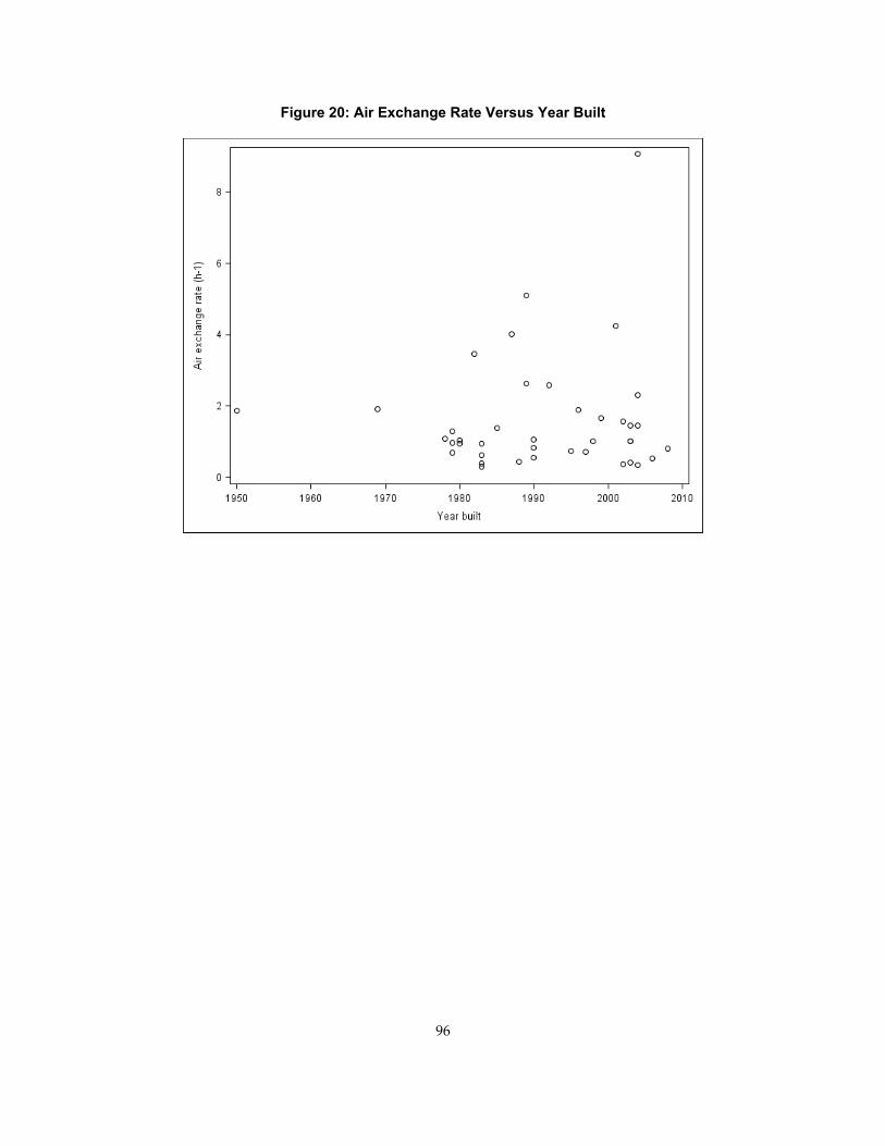
Figure 20: Air Exchange Rate Versus Year Built 

 

96 

 

 

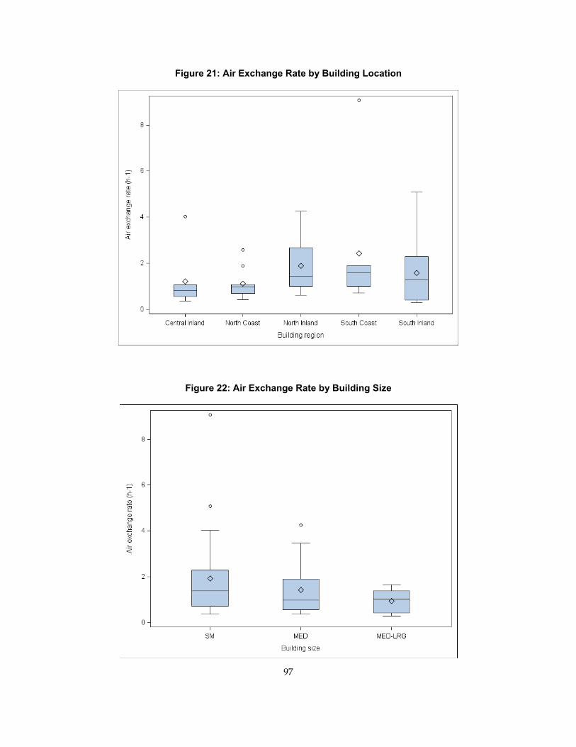
Figure 21: Air Exchange Rate by Building Location 

 

 

Figure 22: Air Exchange Rate by Building Size 

 97 

 

 

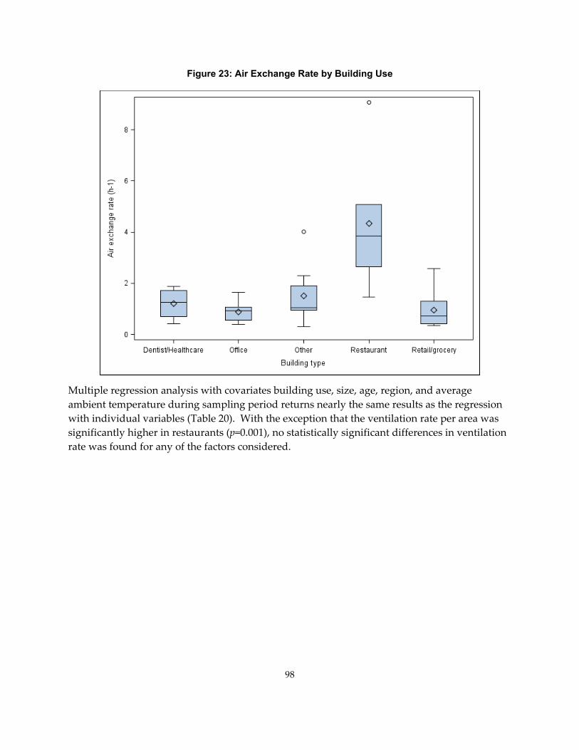
Figure 23: Air Exchange Rate by Building Use

 

Multiple regression analysis with covariates building use, size, age, region, and average ambient temperature during sampling period returns nearly the same results as the regression with individual variables (Table 20).  With the exception that the ventilation rate per area was significantly higher in restaurants (p=0.001), no statistically significant differences in ventilation rate was found for any of the factors considered. 

98 

 

 

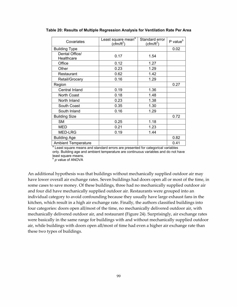
Table 20: Results of Multiple Regression Analysis for Ventilation Rate Per Area 

Covariates Least square meana (cfm/ft2)

Standard error (cfm/ft2) P valueb

Building Type 0.02 Dental Office/

Healthcare 0.17 1.54

Office 0.12 1.27 Other 0.23 1.29 Restaurant 0.62 1.42 Retail/Grocery 0.16 1.29

Region 0.27 Central Inland 0.19 1.36 North Coast 0.18 1.48 North Inland 0.23 1.38 South Coast 0.35 1.30 South Inland 0.16 1.29

Building Size 0.72 SM 0.25 1.18 MED 0.21 1.23 MED-LRG 0.19 1.44

Building Age 0.82 Ambient Temperature 0.41

a Least square means and standard errors are presented for categorical variables only. Building age and ambient temperature are continuous variables and do not have least square means. b p value of ANOVA 

 

An additional hypothesis was that buildings without mechanically supplied outdoor air may have lower overall air exchange rates. Seven buildings had doors open all or most of the time, in some cases to save money. Of these buildings, three had no mechanically supplied outdoor air and four did have mechanically supplied outdoor air. Restaurants were grouped into an individual category to avoid confounding because they usually have large exhaust fans in the kitchen, which result in a high air exchange rate. Finally, the authors classified buildings into four categories: doors open all/most of the time, no mechanically delivered outdoor air, with mechanically delivered outdoor air, and restaurant (Figure 24). Surprisingly, air exchange rates were basically in the same range for buildings with and without mechanically supplied outdoor air, while buildings with doors open all/most of time had even a higher air exchange rate than these two types of buildings. 

99 

 

 

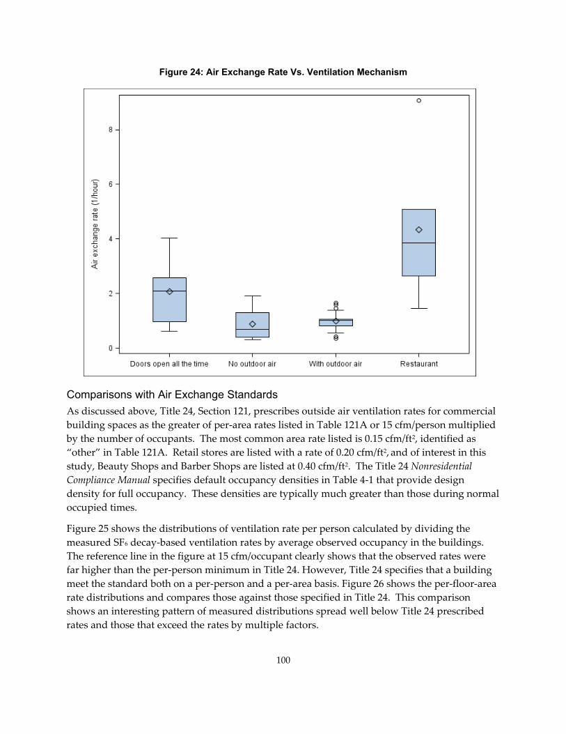
Figure 24: Air Exchange Rate Vs. Ventilation Mechanism

   

Comparisons with Air Exchange Standards As discussed above, Title 24, Section 121, prescribes outside air ventilation rates for commercial building spaces as the greater of per‐area rates listed in Table 121A or 15 cfm/person multiplied by the number of occupants.  The most common area rate listed is 0.15 cfm/ft2, identified as “other” in Table 121A.  Retail stores are listed with a rate of 0.20 cfm/ft2, and of interest in this study, Beauty Shops and Barber Shops are listed at 0.40 cfm/ft2.  The Title 24 Nonresidential Compliance Manual specifies default occupancy densities in Table 4‐1 that provide design density for full occupancy.  These densities are typically much greater than those during normal occupied times.   

Figure 25 shows the distributions of ventilation rate per person calculated by dividing the measured SF6 decay‐based ventilation rates by average observed occupancy in the buildings.  The reference line in the figure at 15 cfm/occupant clearly shows that the observed rates were far higher than the per‐person minimum in Title 24. However, Title 24 specifies that a building meet the standard both on a per‐person and a per‐area basis. Figure 26 shows the per‐floor‐area rate distributions and compares those against those specified in Title 24.  This comparison shows an interesting pattern of measured distributions spread well below Title 24 prescribed rates and those that exceed the rates by multiple factors. 

 100 

 

 

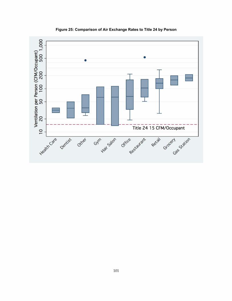
Figure 25: Comparison of Air Exchange Rates to Title 24 by Person

101 

 

 

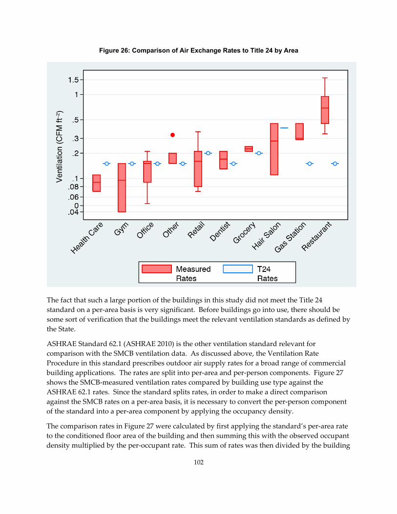
Figure 26: Comparison of Air Exchange Rates to Title 24 by Area

The fact that such a large portion of the buildings in this study did not meet the Title 24 standard on a per‐area basis is very significant.  Before buildings go into use, there should be some sort of verification that the buildings meet the relevant ventilation standards as defined by the State. 

ASHRAE Standard 62.1 (ASHRAE 2010) is the other ventilation standard relevant for comparison with the SMCB ventilation data.  As discussed above, the Ventilation Rate Procedure in this standard prescribes outdoor air supply rates for a broad range of commercial building applications.  The rates are split into per‐area and per‐person components.  Figure 27 shows the SMCB‐measured ventilation rates compared by building use type against the ASHRAE 62.1 rates.  Since the standard splits rates, in order to make a direct comparison against the SMCB rates on a per‐area basis, it is necessary to convert the per‐person component of the standard into a per‐area component by applying the occupancy density.   

The comparison rates in Figure 27 were calculated by first applying the standard’s per‐area rate to the conditioned floor area of the building and then summing this with the observed occupant density multiplied by the per‐occupant rate.  This sum of rates was then divided by the building 

102 

 

 

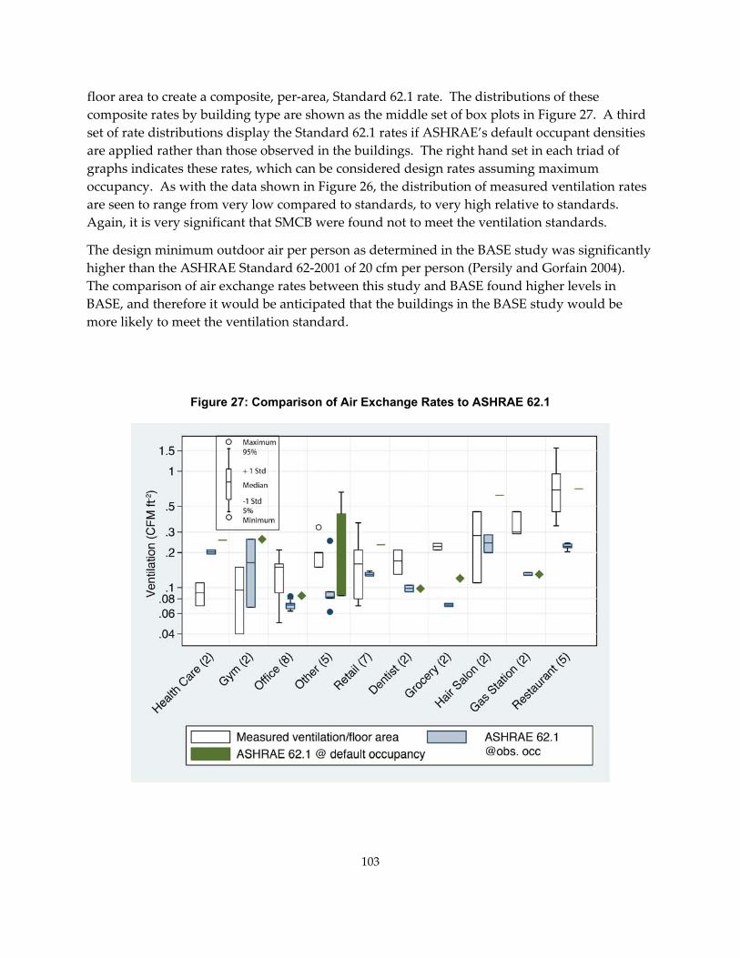
floor area to create a composite, per‐area, Standard 62.1 rate.  The distributions of these composite rates by building type are shown as the middle set of box plots in Figure 27.  A third set of rate distributions display the Standard 62.1 rates if ASHRAE’s default occupant densities are applied rather than those observed in the buildings.  The right hand set in each triad of graphs indicates these rates, which can be considered design rates assuming maximum occupancy.  As with the data shown in Figure 26, the distribution of measured ventilation rates are seen to range from very low compared to standards, to very high relative to standards. Again, it is very significant that SMCB were found not to meet the ventilation standards. 

The design minimum outdoor air per person as determined in the BASE study was significantly higher than the ASHRAE Standard 62‐2001 of 20 cfm per person (Persily and Gorfain 2004).  The comparison of air exchange rates between this study and BASE found higher levels in BASE, and therefore it would be anticipated that the buildings in the BASE study would be more likely to meet the ventilation standard.   

 

 

Figure 27: Comparison of Air Exchange Rates to ASHRAE 62.1

103 

 

 

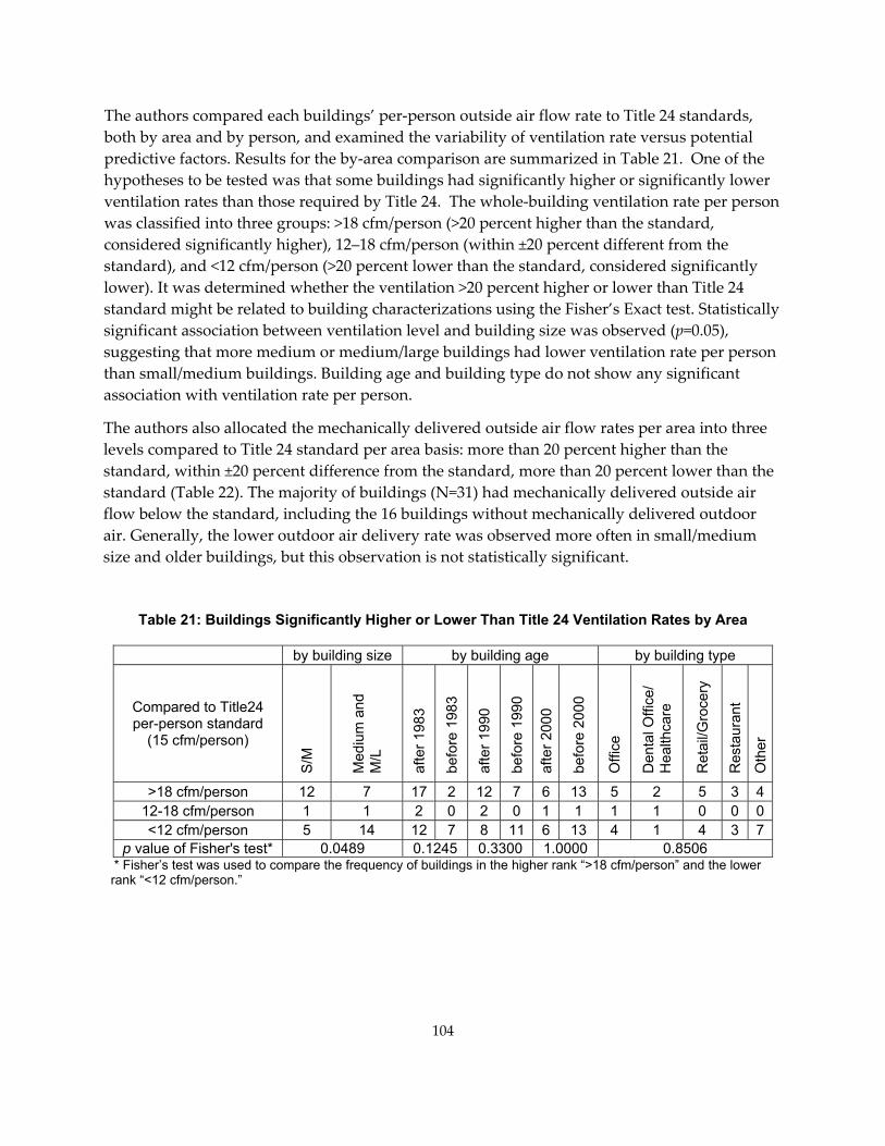
The authors compared each buildings’ per‐person outside air flow rate to Title 24 standards, both by area and by person, and examined the variability of ventilation rate versus potential predictive factors. Results for the by‐area comparison are summarized in Table 21.  One of the hypotheses to be tested was that some buildings had significantly higher or significantly lower ventilation rates than those required by Title 24.  The whole‐building ventilation rate per person was classified into three groups: >18 cfm/person (>20 percent higher than the standard, considered significantly higher), 12–18 cfm/person (within ±20 percent different from the standard), and <12 cfm/person (>20 percent lower than the standard, considered significantly lower). It was determined whether the ventilation >20 percent higher or lower than Title 24 standard might be related to building characterizations using the Fisher’s Exact test. Statistically significant association between ventilation level and building size was observed (p=0.05), suggesting that more medium or medium/large buildings had lower ventilation rate per person than small/medium buildings. Building age and building type do not show any significant association with ventilation rate per person.   

The authors also allocated the mechanically delivered outside air flow rates per area into three levels compared to Title 24 standard per area basis: more than 20 percent higher than the standard, within ±20 percent difference from the standard, more than 20 percent lower than the standard (Table 22). The majority of buildings (N=31) had mechanically delivered outside air flow below the standard, including the 16 buildings without mechanically delivered outdoor air. Generally, the lower outdoor air delivery rate was observed more often in small/medium size and older buildings, but this observation is not statistically significant. 

 

Table 21: Buildings Significantly Higher or Lower Than Title 24 Ventilation Rates by Area 

by building size by building age by building type

Compared to Title24 per-person standard

(15 cfm/person)

S/M

Med

ium

and

M

/L

afte

r 198

3

befo

re 1

983

afte

r 199

0

befo

re 1

990

afte

r 200

0

befo

re 2

000

Offi

ce

Den

tal O

ffice

/ H

ealth

care

Ret

ail/G

roce

ry

Res

taur

ant

Oth

er

>18 cfm/person 12 7 17 2 12 7 6 13 5 2 5 3 412-18 cfm/person 1 1 2 0 2 0 1 1 1 1 0 0 0<12 cfm/person 5 14 12 7 8 11 6 13 4 1 4 3 7

p value of Fisher's test* 0.0489 0.1245 0.3300 1.0000 0.8506  * Fisher’s test was used to compare the frequency of buildings in the higher rank “>18 cfm/person” and the lower rank “<12 cfm/person.” 

104 

 

 

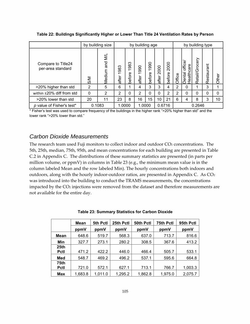
Table 22: Buildings Significantly Higher or Lower Than Title 24 Ventilation Rates by Person

   by building size by building age by building type

Compare to Title24 per-area standard

S/M

Med

ium

and

M/L

afte

r 198

3

befo

re 1

983

afte

r 199

0

befo

re 1

990

afte

r 200

0

befo

re 2

000

Offi

ce

Den

tal o

ffice

/ H

ealth

care

Ret

ail/G

roce

ry

Res

taur

ant

Oth

er

>20% higher than std 2 5 6 1 4 3 3 4 2 0 1 3 1 within ±20% diff from std 0 2 2 0 2 0 0 2 2 0 0 0 0

>20% lower than std 20 11 23 8 16 15 10 21 6 4 8 3 10 p value of Fisher's test* 0.1083 1.0000 1.0000 0.6716 0.2646

* Fisher’s test was used to compare frequency of the buildings in the higher rank “>20% higher than std” and the lower rank “>20% lower than std.” 

Carbon Dioxide Measurements The research team used Fuji monitors to collect indoor and outdoor CO2 concentrations.  The 5th, 25th, median, 75th, 95th, and mean concentrations for each building are presented in Table C.2 in Appendix C.  The distributions of these summary statistics are presented (in parts per million volume, or ppmV) in columns in Table 23 (e.g., the minimum mean value is in the column labeled Mean and the row labeled Min). The hourly concentrations both indoors and outdoors, along with the hourly indoor‐outdoor ratios, are presented in Appendix C.  As CO2 was introduced into the building to conduct the TRAMS measurements, the concentrations impacted by the CO2 injections were removed from the dataset and therefore measurements are not available for the entire day.   

Table 23: Summary Statistics for Carbon Dioxide

Mean 5th Pctl 25th Pctl 50th Pctl 75th Pctl 95th Pctl ppmV ppmV ppmV ppmV ppmV ppmV

Mean 648.6 519.7 568.3 637.0 713.7 816.6 Min 327.7 273.1 280.2 308.5 367.6 413.2 25th Pctl 471.2 422.2 446.0 466.4 505.7 533.1 Med 548.7 469.2 496.2 537.1 595.6 664.8 75th Pctl 721.0 572.1 627.1 713.1 766.7 1,003.3 Max 1,683.8 1,011.0 1,295.2 1,862.8 1,975.0 2,075.7

 

105 

 

 

 

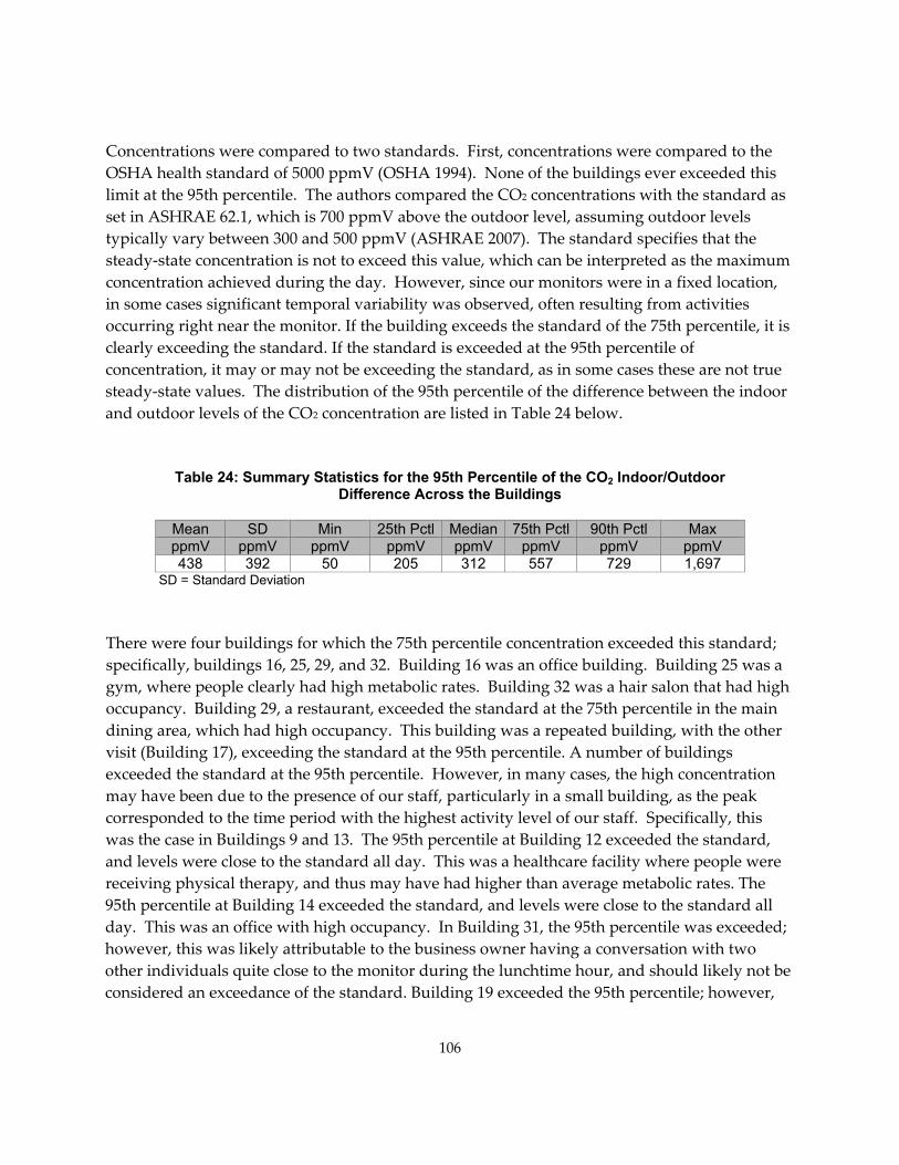
Concentrations were compared to two standards.  First, concentrations were compared to the OSHA health standard of 5000 ppmV (OSHA 1994).  None of the buildings ever exceeded this limit at the 95th percentile.  The authors compared the CO2 concentrations with the standard as set in ASHRAE 62.1, which is 700 ppmV above the outdoor level, assuming outdoor levels typically vary between 300 and 500 ppmV (ASHRAE 2007).  The standard specifies that the steady‐state concentration is not to exceed this value, which can be interpreted as the maximum concentration achieved during the day.  However, since our monitors were in a fixed location, in some cases significant temporal variability was observed, often resulting from activities occurring right near the monitor. If the building exceeds the standard of the 75th percentile, it is clearly exceeding the standard. If the standard is exceeded at the 95th percentile of concentration, it may or may not be exceeding the standard, as in some cases these are not true steady‐state values.  The distribution of the 95th percentile of the difference between the indoor and outdoor levels of the CO2 concentration are listed in Table 24 below.  

 

Table 24: Summary Statistics for the 95th Percentile of the CO2 Indoor/Outdoor Difference Across the Buildings

Mean SD Min 25th Pctl Median 75th Pctl 90th Pctl Max ppmV ppmV ppmV ppmV ppmV ppmV ppmV ppmV 438 392 50 205 312 557 729 1,697

SD = Standard Deviation   

There were four buildings for which the 75th percentile concentration exceeded this standard; specifically, buildings 16, 25, 29, and 32.  Building 16 was an office building.  Building 25 was a gym, where people clearly had high metabolic rates.  Building 32 was a hair salon that had high occupancy.  Building 29, a restaurant, exceeded the standard at the 75th percentile in the main dining area, which had high occupancy.  This building was a repeated building, with the other visit (Building 17), exceeding the standard at the 95th percentile. A number of buildings exceeded the standard at the 95th percentile.  However, in many cases, the high concentration may have been due to the presence of our staff, particularly in a small building, as the peak corresponded to the time period with the highest activity level of our staff.  Specifically, this was the case in Buildings 9 and 13.  The 95th percentile at Building 12 exceeded the standard, and levels were close to the standard all day.  This was a healthcare facility where people were receiving physical therapy, and thus may have had higher than average metabolic rates. The 95th percentile at Building 14 exceeded the standard, and levels were close to the standard all day.  This was an office with high occupancy.  In Building 31, the 95th percentile was exceeded; however, this was likely attributable to the business owner having a conversation with two other individuals quite close to the monitor during the lunchtime hour, and should likely not be considered an exceedance of the standard. Building 19 exceeded the 95th percentile; however, 

106 

 

 

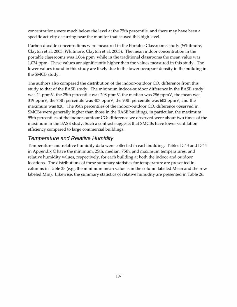
concentrations were much below the level at the 75th percentile, and there may have been a specific activity occurring near the monitor that caused this high level.  

Carbon dioxide concentrations were measured in the Portable Classrooms study (Whitmore, Clayton et al. 2003; Whitmore, Clayton et al. 2003).  The mean indoor concentration in the portable classrooms was 1,064 ppm, while in the traditional classrooms the mean value was 1,074 ppm.  These values are significantly higher than the values measured in this study.  The lower values found in this study are likely due to the lower occupant density in the building in the SMCB study. 

The authors also compared the distribution of the indoor‐outdoor CO2 difference from this study to that of the BASE study.  The minimum indoor‐outdoor difference in the BASE study was 24 ppmV, the 25th percentile was 208 ppmV, the median was 286 ppmV, the mean was 319 ppmV, the 75th percentile was 407 ppmV, the 90th percentile was 602 ppmV, and the maximum was 820.  The 95th percentiles of the indoor‐outdoor CO2 difference observed in SMCBs were generally higher than those in the BASE buildings, in particular, the maximum 95th percentiles of the indoor‐outdoor CO2 difference we observed were about two times of the maximum in the BASE study. Such a contrast suggests that SMCBs have lower ventilation efficiency compared to large commercial buildings.  

Temperature and Relative Humidity Temperature and relative humidity data were collected in each building.  Tables D.43 and D.44 in Appendix C have the minimum, 25th, median, 75th, and maximum temperatures, and relative humidity values, respectively, for each building at both the indoor and outdoor locations.  The distributions of these summary statistics for temperature are presented in columns in Table 25 (e.g., the minimum mean value is in the column labeled Mean and the row labeled Min).  Likewise, the summary statistics of relative humidity are presented in Table 26. 

 

107 

 

 

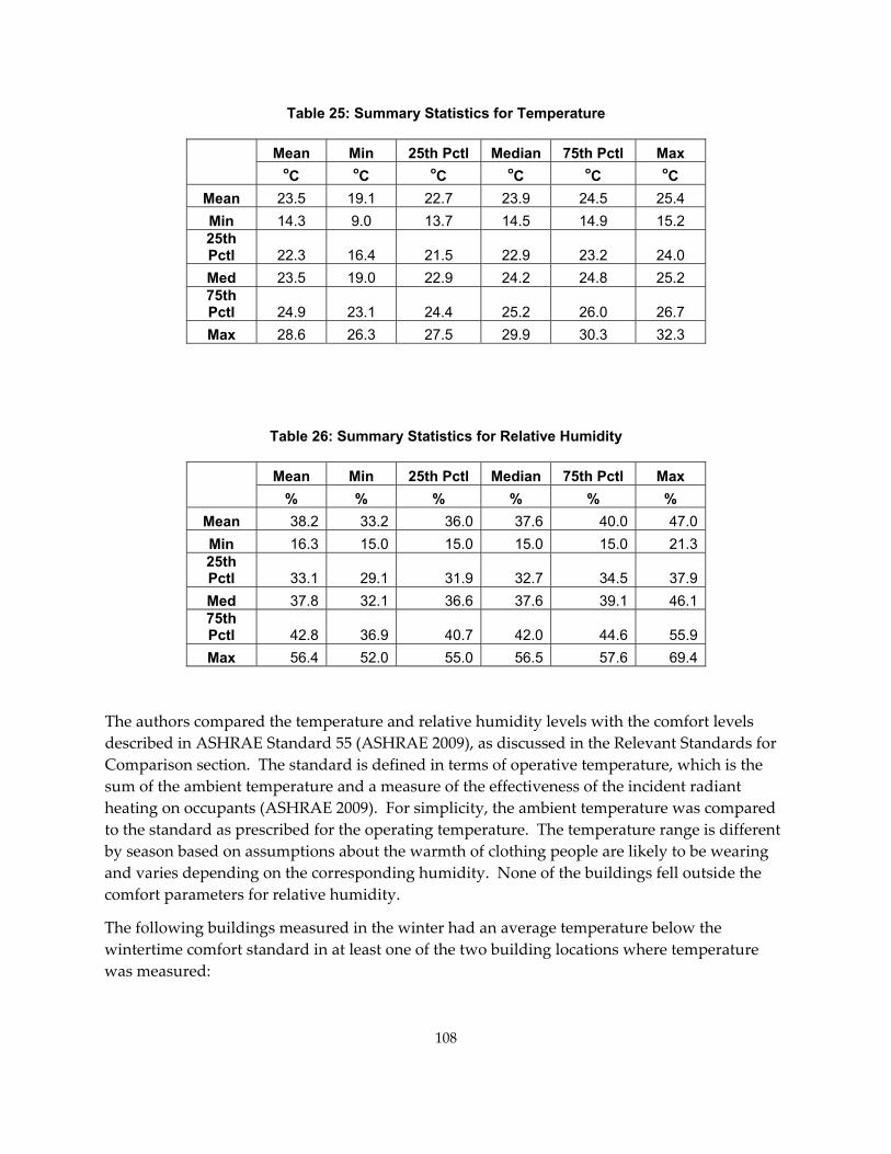
Table 25: Summary Statistics for Temperature

Mean Min 25th Pctl Median 75th Pctl Max

oC oC oC oC oC oC Mean 23.5 19.1 22.7 23.9 24.5 25.4 Min 14.3 9.0 13.7 14.5 14.9 15.2 25th Pctl 22.3 16.4 21.5 22.9 23.2 24.0 Med 23.5 19.0 22.9 24.2 24.8 25.2 75th Pctl 24.9 23.1 24.4 25.2 26.0 26.7 Max 28.6 26.3 27.5 29.9 30.3 32.3

Table 26: Summary Statistics for Relative Humidity

Mean Min 25th Pctl Median 75th Pctl Max

% % % % % % Mean 38.2 33.2 36.0 37.6 40.0 47.0 Min 16.3 15.0 15.0 15.0 15.0 21.3 25th Pctl 33.1 29.1 31.9 32.7 34.5 37.9 Med 37.8 32.1 36.6 37.6 39.1 46.1 75th Pctl 42.8 36.9 40.7 42.0 44.6 55.9 Max 56.4 52.0 55.0 56.5 57.6 69.4

The authors compared the temperature and relative humidity levels with the comfort levels described in ASHRAE Standard 55 (ASHRAE 2009), as discussed in the Relevant Standards for Comparison section.  The standard is defined in terms of operative temperature, which is the sum of the ambient temperature and a measure of the effectiveness of the incident radiant heating on occupants (ASHRAE 2009).  For simplicity, the ambient temperature was compared to the standard as prescribed for the operating temperature.  The temperature range is different by season based on assumptions about the warmth of clothing people are likely to be wearing and varies depending on the corresponding humidity.  None of the buildings fell outside the comfort parameters for relative humidity. 

The following buildings measured in the winter had an average temperature below the wintertime comfort standard in at least one of the two building locations where temperature was measured:  

108 

 

 

• Building 2, a grocery store (1 of 2 locations). The lower temperature was most likely intended to preserve food freshness and for energy efficiency due to the refrigerated cases located in the grocery store. 

• Building 25, a gym (in the 1 measured location). The lower temperature was most likely because it is more comfortable for patrons to exercise in a cooler environment. 

• Building 29, a restaurant (in 1 of 2 locations). The kitchen was the cool location.  

• Building 34, a retail‐bookstore (in the 1 measured location).  The outdoor temperature was very cold, and this building was purposely kept cool to save money on heating bills. 

• Building 36, a grocery store (both locations).  The lower temperature was most likely to preserve food freshness and for energy efficiency due to the refrigerated cases located in the grocery store. 

The following buildings measured in the winter had temperatures above the wintertime comfort standard:  

• Building 5, an office (1 of 2 locations). The warmer area was a small storage area with a photocopy machine, and thus not regularly occupied by employees.  From a comfort perspective, this elevated temperature is not particularly relevant.  

• Building 6, a retail skate/clothing shop (in both locations). Because outdoor temperatures were very high, it would be more appropriate to use the summertime standard for this building, and the temperature was within the summertime standard.   

• Building 7, a gas station (the 1 measured location). Outdoor temperatures were very high, so it would be more appropriate to use the summertime standard for this building, and the temperature was within the summertime standard.   

The following buildings measured in the summer had temperatures below the summertime comfort standard:  

• Building 8, a religious worship building (both locations) Outdoor temperatures were very low, so it is likely that the wintertime standard should be used for this building, and the temperatures were within the wintertime comfort standard.   

• Building 15, an office (1 of 2 locations). The HVAC system appears to overcool the space. 

• Building 19, an office (the 1 measured location). The HVAC system appears to overcool the space. 

• Building 21, a government building (1 of 2 locations) The HVAC system appears to overcool the space. 

• Building 23, an office (1 of 2 locations). The HVAC system appears to overcool the space.  In addition, the building operator noted that he manipulated the temperatures to provide warmer and cooler areas and allowed people to select offices in the warmer or cooler areas, depending on their temperature preference.   

109 

 

 

The following buildings measured in the summer had temperatures above the summertime comfort standard:  

• Building 18, a gym (in 1 of 2 locations). 

• Building 20, a water retailer (in both locations). The building operator relied primarily on natural ventilation and no thermal conditioning, and it was a warm day.  

• Building 22, a daycare (the 1 measured location). The building operator relied primarily on natural ventilation and no thermal conditioning, and it was a warm day.  

 

In terms of energy usage, the most significant finding is that buildings are overcooling in the summertime, which was found in three of the offices and in one government service building, which also included office space.  There were eight offices (including the one government services building) measured during the summer, so of the offices, a significant fraction were overcooled.  A similar finding was found in the BASE study, which only considered office buildings, so this is not a surprising finding (Persily and Gorfain 2004).  One new finding from this study is that overcooling did not appear to occur in any of the other building types. 

Indoor Air Quality This study measured a suite of criteria air pollutants and toxic air pollutants.  The criteria air pollutant measurements included real‐time measurements of CO, multiple‐ size fractions of particulate matter, and ultrafine particles.  Integrated measurements of PM2.5 and PM10 were also collected over the 8‐hour sampling period.  The toxic air pollutants included many VOCs and aldehydes commonly found indoors, many of which are thought to cause adverse health effects. These were measured using an integrated sampler over a four‐hour time period.  All above samples were measured both outdoors and indoors, with the integrated measures and the real‐time PM being collected in two locations indoors in the larger buildings. Finally, real‐time measurements of black carbon were collected both indoors and outdoors, at street level and on the roof, to determine the fraction of particles of outdoor origin penetrating the building.  Information on the history of water damage and occupant complaints were also collected. 

Criteria Air Pollutants Carbon Monoxide The research team used two Q‐Track monitors to measure CO concentrations.  They were distributed between the indoor and outdoor locations.  Unfortunately, while regular calibrations of the CO monitors were conducted, the data recorded during the project were not checked, as this pollutant was of lower priority.  One Q‐Track appears to have had limited sensitivity at low concentrations as compared to the other, as one Q‐Track rarely recorded values other than zero.  Therefore, only summary statistics for indoor concentrations measured with the more sensitive Q‐Track are presented in Appendix C, Table C.45.  In summary, most buildings were below the limit of detection.  The highest level was at a building providing auto 

110 

 

 

services, with an average of 4.6 ppmV and a 95th percentile of 5.4 ppmV, approximately 50 percent below any health‐based standard.  The next highest average concentration was 2.0 ppmV, with a 95th percentile of 2.5 ppmV, at a restaurant.  Unfortunately, due to the limitations of the Q‐Track monitors used, little can be concluded in regard to levels of CO typically found in SMCB in California. 

Real-Time Particulate Matter Measures The research team used Met One 237AB instruments to sample real‐time PM concentrations at different size fractions at each designated sample site for the building. The approximate mass in each of the following size fractions was calculated:  0.3 μm to 0.5 μm, 0.5 μm to 0.7 μm, 0.7 μm to 1.0 μm, 1.0 μm to 2.0 μm, and 2.0 μm to 5.0 μm.  In addition, the mass in all size fractions below PM2.0 were summed to determine the approximate PM2.0 mass.  

PM2.0 mass is estimated and plotted against time using a 10‐minute moving average, allowing one to understand the temporal profile for all the buildings in the study.  Bar charts of the distribution of the mass in each size fraction over the course of the day were prepared, allowing determination of the relative contribution of the various size fractions and comparison of the differences between indoor and outdoor levels.  All of these results are presented in Appendix E.  Summary statistics for each building in each size fraction are also calculated and presented in Table C.46, in Appendix C.  Note that because of the way that the mass was calculated, mass estimates are meant just for comparative purposes. 

Summary statistics of the mean concentration of the indoor particle concentration for each size fraction are summarized in Table 27 for all buildings, as well as by building type. Note that due to the small sample size for particular types of buildings, the maximum, not the 95th percentile, is presented in the statistical summary by building type.  

Figure 28 is the box plot of indoor PM concentrations by building type. As shown in the figure, dental office and hair salons had relatively high particle concentrations compared to other types of buildings.  The dental practices (e.g., drilling and polishing, and the aerosolized saliva emitted from patients’ mouths during treatment) may cause elevated particle level indoors (Helmis, Tzoutzas et al. 2007; Sotiriou, Ferguson et al. 2008). Studies on particle level in hair salons are very limited. However, research has found that use of hair appliances such as hair dryers, curling irons, and hair straighteners could increase indoor particle levels (Wallace and Ott 2011). In addition, other potential sources in hair salons (e.g., small pieces of hair, particles resuspended while sweeping the floor, and particles generated during oxidation reactions occurring on the hair from products containing compounds such as d‐limonene) may also contribute to indoor particle level. Further studies are required to confirm the presence of these sources. 

111 

 

 

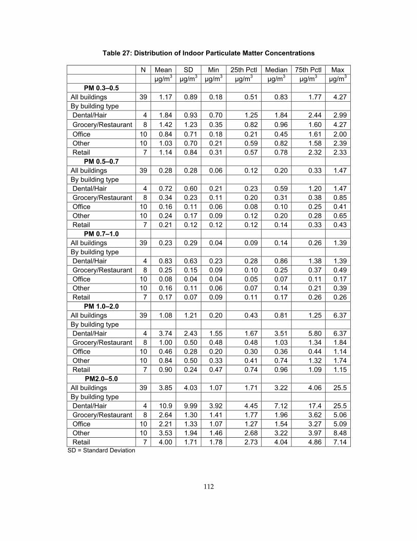
Table 27: Distribution of Indoor Particulate Matter Concentrations

N Mean SD Min 25th Pctl Median 75th Pctl Max μg/m3 μg/m3 µg/m3 µg/m3 µg/m3 µg/m3 µg/m3

PM 0.3–0.5 All buildings 39 1.17 0.89 0.18 0.51 0.83 1.77 4.27By building type Dental/Hair 4 1.84 0.93 0.70 1.25 1.84 2.44 2.99 Grocery/Restaurant 8 1.42 1.23 0.35 0.82 0.96 1.60 4.27 Office 10 0.84 0.71 0.18 0.21 0.45 1.61 2.00 Other 10 1.03 0.70 0.21 0.59 0.82 1.58 2.39 Retail 7 1.14 0.84 0.31 0.57 0.78 2.32 2.33

PM 0.5–0.7 All buildings 39 0.28 0.28 0.06 0.12 0.20 0.33 1.47By building type Dental/Hair 4 0.72 0.60 0.21 0.23 0.59 1.20 1.47 Grocery/Restaurant 8 0.34 0.23 0.11 0.20 0.31 0.38 0.85 Office 10 0.16 0.11 0.06 0.08 0.10 0.25 0.41 Other 10 0.24 0.17 0.09 0.12 0.20 0.28 0.65 Retail 7 0.21 0.12 0.12 0.12 0.14 0.33 0.43

PM 0.7–1.0 All buildings 39 0.23 0.29 0.04 0.09 0.14 0.26 1.39By building type Dental/Hair 4 0.83 0.63 0.23 0.28 0.86 1.38 1.39 Grocery/Restaurant 8 0.25 0.15 0.09 0.10 0.25 0.37 0.49 Office 10 0.08 0.04 0.04 0.05 0.07 0.11 0.17 Other 10 0.16 0.11 0.06 0.07 0.14 0.21 0.39 Retail 7 0.17 0.07 0.09 0.11 0.17 0.26 0.26

PM 1.0–2.0 All buildings 39 1.08 1.21 0.20 0.43 0.81 1.25 6.37By building type Dental/Hair 4 3.74 2.43 1.55 1.67 3.51 5.80 6.37 Grocery/Restaurant 8 1.00 0.50 0.48 0.48 1.03 1.34 1.84 Office 10 0.46 0.28 0.20 0.30 0.36 0.44 1.14 Other 10 0.84 0.50 0.33 0.41 0.74 1.32 1.74 Retail 7 0.90 0.24 0.47 0.74 0.96 1.09 1.15

PM2.0–5.0 All buildings 39 3.85 4.03 1.07 1.71 3.22 4.06 25.5By building type Dental/Hair 4 10.9 9.99 3.92 4.45 7.12 17.4 25.5 Grocery/Restaurant 8 2.64 1.30 1.41 1.77 1.96 3.62 5.06 Office 10 2.21 1.33 1.07 1.27 1.54 3.27 5.09 Other 10 3.53 1.94 1.46 2.68 3.22 3.97 8.48 Retail 7 4.00 1.71 1.78 2.73 4.04 4.86 7.14

SD = Standard Deviation

112 

 

 

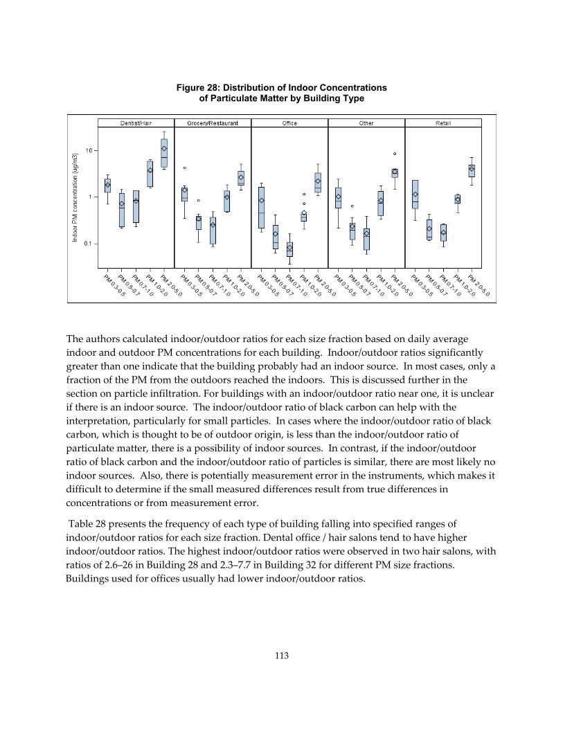
Figure 28: Distribution of Indoor Concentrations of Particulate Matter by Building Type 

 

 

The authors calculated indoor/outdoor ratios for each size fraction based on daily average indoor and outdoor PM concentrations for each building.  Indoor/outdoor ratios significantly greater than one indicate that the building probably had an indoor source.  In most cases, only a fraction of the PM from the outdoors reached the indoors.  This is discussed further in the section on particle infiltration. For buildings with an indoor/outdoor ratio near one, it is unclear if there is an indoor source.  The indoor/outdoor ratio of black carbon can help with the interpretation, particularly for small particles.  In cases where the indoor/outdoor ratio of black carbon, which is thought to be of outdoor origin, is less than the indoor/outdoor ratio of particulate matter, there is a possibility of indoor sources.  In contrast, if the indoor/outdoor ratio of black carbon and the indoor/outdoor ratio of particles is similar, there are most likely no indoor sources.  Also, there is potentially measurement error in the instruments, which makes it difficult to determine if the small measured differences result from true differences in concentrations or from measurement error. 

 Table 28 presents the frequency of each type of building falling into specified ranges of indoor/outdoor ratios for each size fraction. Dental office / hair salons tend to have higher indoor/outdoor ratios. The highest indoor/outdoor ratios were observed in two hair salons, with ratios of 2.6–26 in Building 28 and 2.3–7.7 in Building 32 for different PM size fractions. Buildings used for offices usually had lower indoor/outdoor ratios.  

113 

 

 

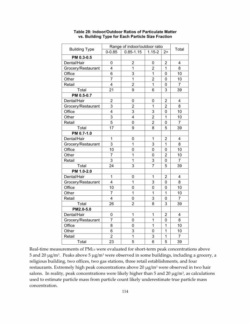
Table 28: Indoor/Outdoor Ratios of Particulate Matter vs. Building Type for Each Particle Size Fraction 

Building Type Range of indoor/outdoor ratio Total 0-0.85 0.85-1.15 1.15-2 2+PM 0.3-0.5

Dental/Hair 0 2 0 2 4 Grocery/Restaurant 4 1 2 1 8 Office 6 3 1 0 10 Other 7 1 2 0 10 Retail 4 2 1 0 7

Total 21 9 6 3 39 PM 0.5-0.7

Dental/Hair 2 0 0 2 4 Grocery/Restaurant 3 2 1 2 8 Office 4 3 3 0 10 Other 3 4 2 1 10 Retail 5 0 2 0 7

Total 17 9 8 5 39 PM 0.7-1.0

Dental/Hair 1 0 1 2 4 Grocery/Restaurant 3 1 3 1 8 Office 10 0 0 0 10 Other 7 1 0 2 10 Retail 3 1 3 0 7

Total 24 3 7 5 39 PM 1.0-2.0

Dental/Hair 1 0 1 2 4 Grocery/Restaurant 4 1 3 0 8 Office 10 0 0 0 10 Other 7 1 1 1 10 Retail 4 0 3 0 7

Total 26 2 8 3 39 PM2.0-5.0

Dental/Hair 0 1 1 2 4 Grocery/Restaurant 7 0 1 0 8 Office 8 0 1 1 10 Other 6 3 0 1 10 Retail 2 1 3 1 7

Total 23 5 6 5 39

Real‐time measurements of PM2.0 were evaluated for short‐term peak concentrations above 5 and 20 μg/m3.  Peaks above 5 μg/m3 were observed in some buildings, including a grocery, a religious building, two offices, two gas stations, three retail establishments, and four restaurants. Extremely high peak concentrations above 20 μg/m3 were observed in two hair salons.  In reality, peak concentrations were likely higher than 5 and 20 μg/m3, as calculations used to estimate particle mass from particle count likely underestimate true particle mass concentration.  

114 

 

 

Unfortunately, there are not many real‐time PM data available for comparison. A few published articles reported measuring real‐time PM (Abt, Suh et al. 2000; Fisk, Faulkner et al. 2000; Long, Suh et al. 2000; Ferro, Kopperud et al. 2004; He, Morawska et al. 2004; Kumar, Chu et al. 2007); however, they either used different instruments or used the number concentration for further analyses but did not report the measured PM concentrations at different size fractions.  

Quality Assurance and Quality Control Results for Real-Time Particulate Matter The authors developed a QA/QC plan based on their expert judgment.  Indoor air concentrations are considerably more variable than outdoor measurements, and different QA/QC procedures are used for indoor air than for outdoor air.  Met One BAM instruments are used throughout the state by ARB (ARB 2008). 

Considering the differences among the Met‐One instruments, the research team conducted co‐location tests on the five instruments used in the field sampling: ME2, ME3, ME4, ME5, and ME9. ME3, ME4, and ME5 were used on a regular basis in the majority of the buildings because the initial co‐locations found that these instruments had the lowest differences between them. ME2 and ME9 were only used at limited times, as backup devices.  

Five collocation tests were conducted, and the instrument readings were compared for each size fraction. Based on the results of co‐location tests, the difference among the five instruments were within ±20 percent for particles with diameters equal to or above 0.3 μm in all tests.  In many cases, there were not clear trends between the instruments over the multiple collocations.  Therefore, based on expert judgment, no correction was made for this size fraction. The samplers with variation within the 20 percent range also did not necessarily show consistent trends.  ME3 overestimated the count of particles with diameters equal to or above 0.5 μm by ~25 percent of the average of other Met‐One instruments in two tests conducted in April 2010, and thus data collected by ME3 since April 2010 were corrected.  

ME5 reported higher readings than other Met‐One instruments for particles with diameters equal to or above 2.0 μm by different percentage in two co‐location tests. Paired indoor samples collected in the field sampling using ME5 and other Met‐One instruments were compared, and it was decided to use the average of the ratio of ME5 to each  other Met‐One instrument to determine how to correct the over‐estimation of ME5. In comparison to other Met‐One instruments used in the study, the backup device, ME9, underestimated particle counts  by ~35 percent for particles with diameters equal to or above 0.5 μm, by ~55 percent for particles with diameters equal to or above 0.7 μm, and by ~65 percent for particles with diameters equal to or above 1.0 μm. It was only used once, in Building 39. In summary, adjustment was made based on the real‐time count data from the above results, and the corrections applied are presented inTable 29. Corrections were made on the count data for particles above the specified size fraction, prior to determining the particle count in a particular range of size fractions. 

115 

 

 

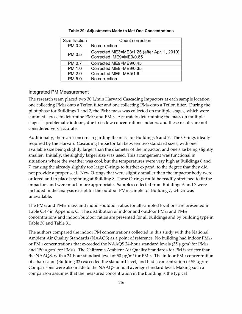
Table 29: Adjustments Made to Met One Concentrations 

Size fraction Count correctionPM 0.3 No correction

PM 0.5 Corrected ME3=ME3/1.25 (after Apr. 1, 2010) Corrected ME9=ME9/0.65

PM 0.7 Corrected ME9=ME9/0.45PM 1.0 Corrected ME9=ME9/0.35PM 2.0 Corrected ME5=ME5/1.6PM 5.0 No correction

Integrated PM Measurement The research team placed two 30 L/min Harvard Cascading Impactors at each sample location; one collecting PM2.5 onto a Teflon filter and one collecting PM10 onto a Teflon filter.  During the pilot phase for Buildings 1 and 2, the PM2.5 mass was collected on multiple stages, which were summed across to determine PM2.5 and PM10.  Accurately determining the mass on multiple stages is problematic indoors, due to its low concentrations indoors, and these results are not considered very accurate.   

Additionally, there are concerns regarding the mass for Buildings 6 and 7.  The O‐rings ideally required by the Harvard Cascading Impactor fall between two standard sizes, with one available size being slightly larger than the diameter of the impactor, and one size being slightly smaller.  Initially, the slightly larger size was used. This arrangement was functional in situations where the weather was cool, but the temperatures were very high at Buildings 6 and 7, causing the already slightly too large O‐rings to further expand, to the degree that they did not provide a proper seal.  New O‐rings that were slightly smaller than the impactor body were ordered and in place beginning at Building 8. These O‐rings could be readily stretched to fit the impactors and were much more appropriate.  Samples collected from Buildings 6 and 7 were included in the analysis except for the outdoor PM10 sample for Building 7, which was unavailable. 

The PM2.5 and PM10  mass and indoor‐outdoor ratios for all sampled locations are presented in Table C.47 in Appendix C.  The distribution of indoor and outdoor PM2.5 and PM10 concentrations and indoor/outdoor ratios are presented for all buildings and by building type in Table 30 and Table 31. 

The authors compared the indoor PM concentrations collected in this study with the National Ambient Air Quality Standards (NAAQS) as a point of reference. No building had indoor PM2.5 or PM10 concentrations that exceeded the NAAQS 24‐hour standard levels (35 μg/m3 for PM2.5 and 150 μg/m3 for PM10).  The California Ambient Air Quality Standards for PM is stricter than the NAAQS, with a 24‐hour standard level of 50 μg/m3 for PM10.  The indoor PM10 concentration of a hair salon (Building 32) exceeded the standard level, and had a concentration of 55 μg/m3.  Comparisons were also made to the NAAQS annual average standard level. Making such a comparison assumes that the measured concentration in the building is the typical 

116 

 

 

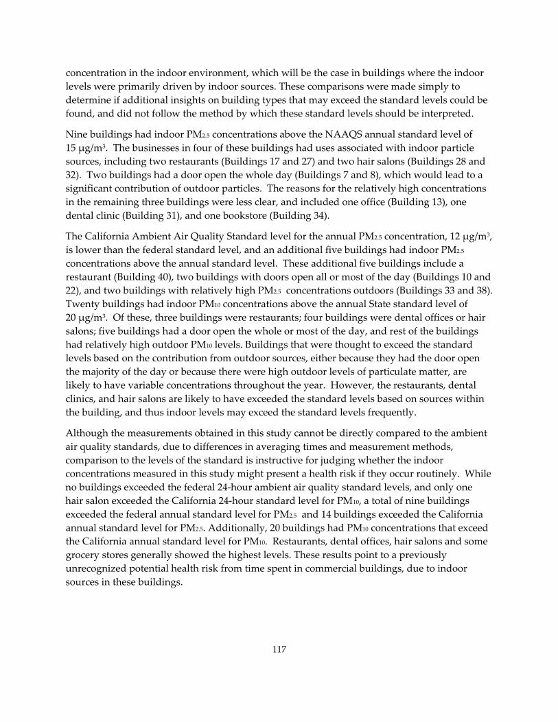
concentration in the indoor environment, which will be the case in buildings where the indoor levels were primarily driven by indoor sources. These comparisons were made simply to determine if additional insights on building types that may exceed the standard levels could be found, and did not follow the method by which these standard levels should be interpreted.   

Nine buildings had indoor PM2.5 concentrations above the NAAQS annual standard level of 15 μg/m3.  The businesses in four of these buildings had uses associated with indoor particle sources, including two restaurants (Buildings 17 and 27) and two hair salons (Buildings 28 and 32).  Two buildings had a door open the whole day (Buildings 7 and 8), which would lead to a significant contribution of outdoor particles.  The reasons for the relatively high concentrations in the remaining three buildings were less clear, and included one office (Building 13), one dental clinic (Building 31), and one bookstore (Building 34).  

The California Ambient Air Quality Standard level for the annual PM2.5 concentration, 12 μg/m3, is lower than the federal standard level, and an additional five buildings had indoor PM2.5 concentrations above the annual standard level.  These additional five buildings include a restaurant (Building 40), two buildings with doors open all or most of the day (Buildings 10 and 22), and two buildings with relatively high PM2.5  concentrations outdoors (Buildings 33 and 38). Twenty buildings had indoor PM10 concentrations above the annual State standard level of 20 μg/m3.  Of these, three buildings were restaurants; four buildings were dental offices or hair salons; five buildings had a door open the whole or most of the day, and rest of the buildings had relatively high outdoor PM10 levels. Buildings that were thought to exceed the standard levels based on the contribution from outdoor sources, either because they had the door open the majority of the day or because there were high outdoor levels of particulate matter, are likely to have variable concentrations throughout the year.  However, the restaurants, dental clinics, and hair salons are likely to have exceeded the standard levels based on sources within the building, and thus indoor levels may exceed the standard levels frequently. 

Although the measurements obtained in this study cannot be directly compared to the ambient air quality standards, due to differences in averaging times and measurement methods, comparison to the levels of the standard is instructive for judging whether the indoor concentrations measured in this study might present a health risk if they occur routinely.  While no buildings exceeded the federal 24‐hour ambient air quality standard levels, and only one hair salon exceeded the California 24‐hour standard level for PM10, a total of nine buildings exceeded the federal annual standard level for PM2.5  and 14 buildings exceeded the California annual standard level for PM2.5. Additionally, 20 buildings had PM10 concentrations that exceed the California annual standard level for PM10.  Restaurants, dental offices, hair salons and some grocery stores generally showed the highest levels. These results point to a previously unrecognized potential health risk from time spent in commercial buildings, due to indoor sources in these buildings. 

117 

 

 

 

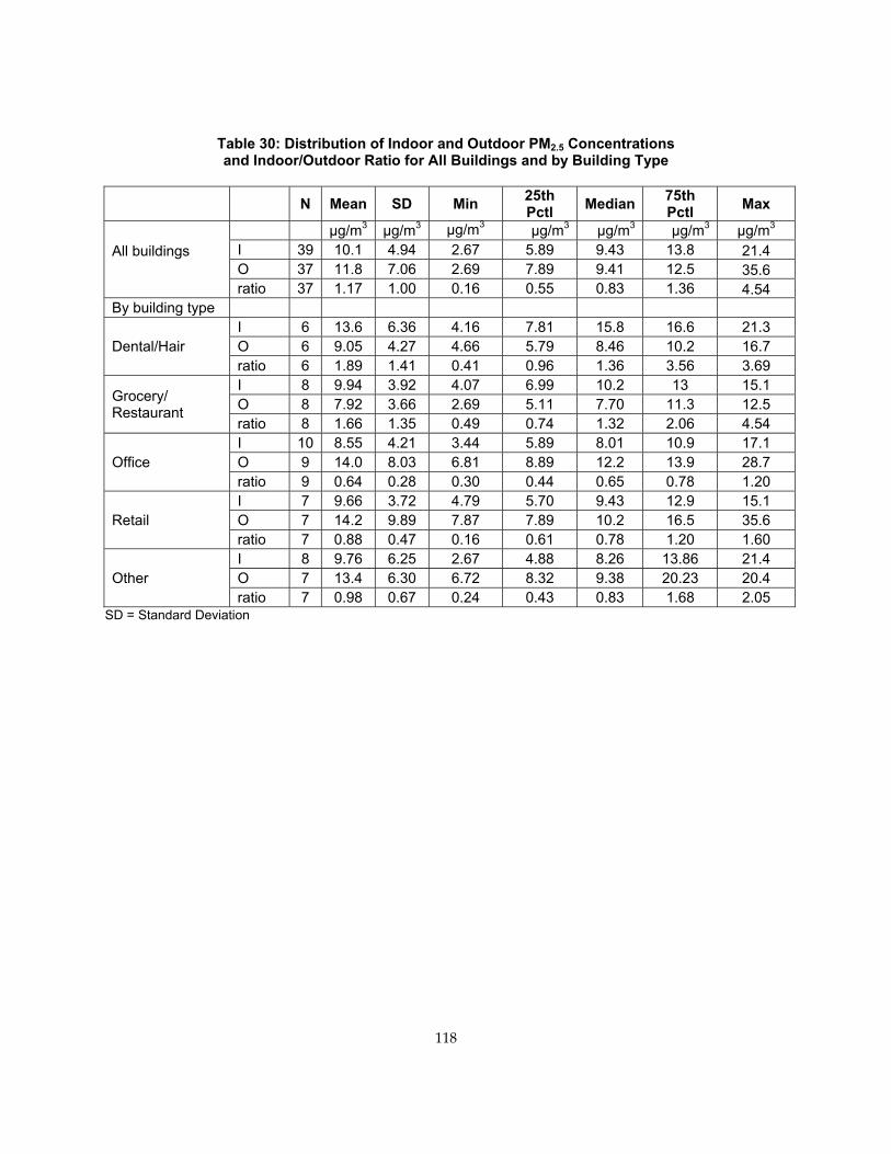
Table 30: Distribution of Indoor and Outdoor PM2.5 Concentrations and Indoor/Outdoor Ratio for All Buildings and by Building Type

SD = Standard Deviation

N Mean SD Min 25th Pctl Median 75th

Pctl Max

All buildings µg/m3 µg/m3 µg/m3 µg/m3 µg/m3 µg/m3 µg/m3 I 39 10.1 4.94 2.67 5.89 9.43 13.8 21.4 O 37 11.8 7.06 2.69 7.89 9.41 12.5 35.6 ratio 37 1.17 1.00 0.16 0.55 0.83 1.36 4.54

By building type

Dental/Hair I 6 13.6 6.36 4.16 7.81 15.8 16.6 21.3 O 6 9.05 4.27 4.66 5.79 8.46 10.2 16.7 ratio 6 1.89 1.41 0.41 0.96 1.36 3.56 3.69

Grocery/ Restaurant

I 8 9.94 3.92 4.07 6.99 10.2 13 15.1 O 8 7.92 3.66 2.69 5.11 7.70 11.3 12.5 ratio 8 1.66 1.35 0.49 0.74 1.32 2.06 4.54

Office I 10 8.55 4.21 3.44 5.89 8.01 10.9 17.1 O 9 14.0 8.03 6.81 8.89 12.2 13.9 28.7 ratio 9 0.64 0.28 0.30 0.44 0.65 0.78 1.20

Retail I 7 9.66 3.72 4.79 5.70 9.43 12.9 15.1 O 7 14.2 9.89 7.87 7.89 10.2 16.5 35.6 ratio 7 0.88 0.47 0.16 0.61 0.78 1.20 1.60

Other I 8 9.76 6.25 2.67 4.88 8.26 13.86 21.4 O 7 13.4 6.30 6.72 8.32 9.38 20.23 20.4 ratio 7 0.98 0.67 0.24 0.43 0.83 1.68 2.05

118 

 

 

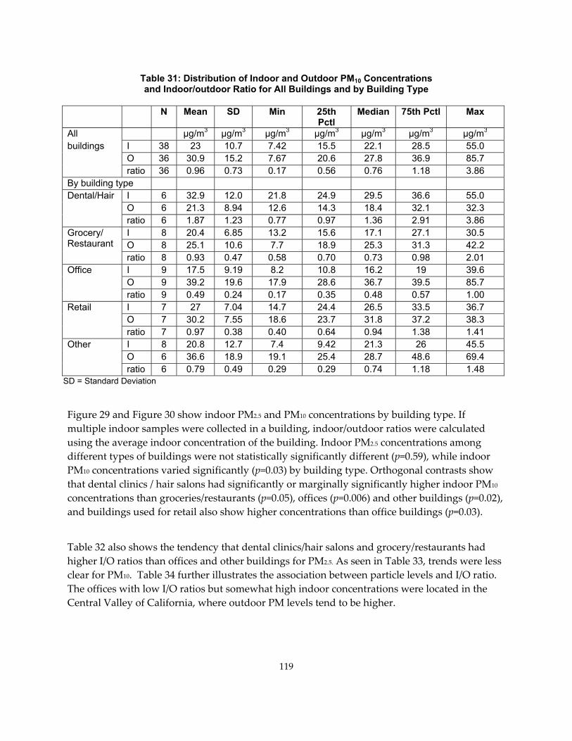
Table 31: Distribution of Indoor and Outdoor PM10 Concentrations and Indoor/outdoor Ratio for All Buildings and by Building Type

N Mean SD Min 25th Pctl

Median 75th Pctl Max

All buildings

µg/m3 µg/m3 µg/m3 µg/m3 µg/m3 µg/m3 µg/m3 I 38 23 10.7 7.42 15.5 22.1 28.5 55.0 O 36 30.9 15.2 7.67 20.6 27.8 36.9 85.7 ratio 36 0.96 0.73 0.17 0.56 0.76 1.18 3.86

By building type Dental/Hair I 6 32.9 12.0 21.8 24.9 29.5 36.6 55.0

O 6 21.3 8.94 12.6 14.3 18.4 32.1 32.3 ratio 6 1.87 1.23 0.77 0.97 1.36 2.91 3.86

Grocery/ Restaurant

I 8 20.4 6.85 13.2 15.6 17.1 27.1 30.5 O 8 25.1 10.6 7.7 18.9 25.3 31.3 42.2 ratio 8 0.93 0.47 0.58 0.70 0.73 0.98 2.01

Office I 9 17.5 9.19 8.2 10.8 16.2 19 39.6 O 9 39.2 19.6 17.9 28.6 36.7 39.5 85.7 ratio 9 0.49 0.24 0.17 0.35 0.48 0.57 1.00

Retail I 7 27 7.04 14.7 24.4 26.5 33.5 36.7 O 7 30.2 7.55 18.6 23.7 31.8 37.2 38.3 ratio 7 0.97 0.38 0.40 0.64 0.94 1.38 1.41

Other I 8 20.8 12.7 7.4 9.42 21.3 26 45.5 O 6 36.6 18.9 19.1 25.4 28.7 48.6 69.4 ratio 6 0.79 0.49 0.29 0.29 0.74 1.18 1.48

SD = Standard Deviation  

Figure 29 and Figure 30 show indoor PM2.5 and PM10 concentrations by building type. If multiple indoor samples were collected in a building, indoor/outdoor ratios were calculated using the average indoor concentration of the building. Indoor PM2.5 concentrations among different types of buildings were not statistically significantly different (p=0.59), while indoor PM10 concentrations varied significantly (p=0.03) by building type. Orthogonal contrasts show that dental clinics / hair salons had significantly or marginally significantly higher indoor PM10 concentrations than groceries/restaurants (p=0.05), offices (p=0.006) and other buildings (p=0.02), and buildings used for retail also show higher concentrations than office buildings (p=0.03). 

 Table 32 also shows the tendency that dental clinics/hair salons and grocery/restaurants had higher I/O ratios than offices and other buildings for PM2.5. As seen in Table 33, trends were less clear for PM10.  Table 34 further illustrates the association between particle levels and I/O ratio.  The offices with low I/O ratios but somewhat high indoor concentrations were located in the Central Valley of California, where outdoor PM levels tend to be higher.   

119 

 

 

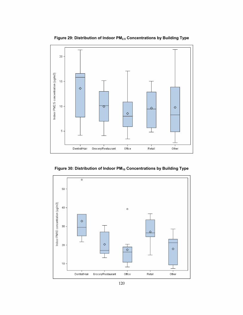
Figure 29: Distribution of Indoor PM2.5 Concentrations by Building Type

 

Figure 30: Distribution of Indoor PM10 Concentrations by Building Type

 120 

 

 

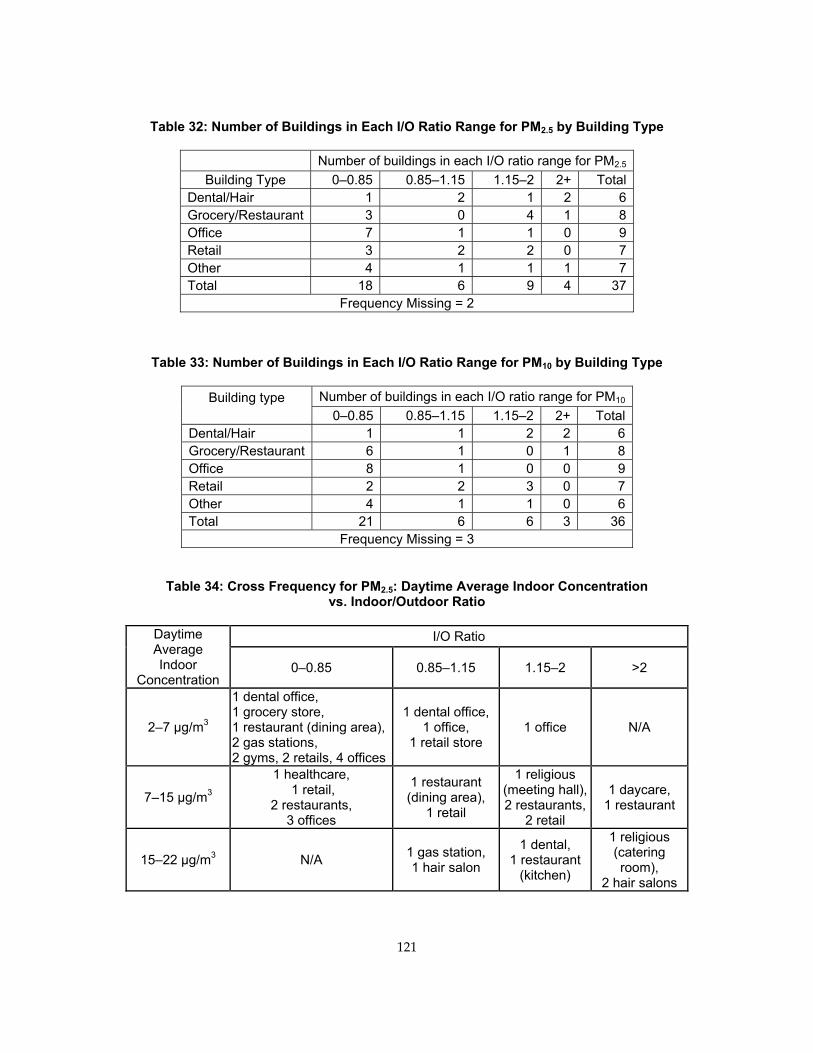
Table 32: Number of Buildings in Each I/O Ratio Range for PM2.5 by Building Type 

Number of buildings in each I/O ratio range for PM2.5 Building Type 0–0.85 0.85–1.15 1.15–2 2+ Total

Dental/Hair 1 2 1 2 6 Grocery/Restaurant 3 0 4 1 8 Office 7 1 1 0 9 Retail 3 2 2 0 7 Other 4 1 1 1 7 Total 18 6 9 4 37

Frequency Missing = 2

Table 33: Number of Buildings in Each I/O Ratio Range for PM10 by Building Type

Building type Number of buildings in each I/O ratio range for PM10 0–0.85 0.85–1.15 1.15–2 2+ Total

Dental/Hair 1 1 2 2 6 Grocery/Restaurant 6 1 0 1 8 Office 8 1 0 0 9 Retail 2 2 3 0 7 Other 4 1 1 0 6 Total 21 6 6 3 36

Frequency Missing = 3  

Table 34: Cross Frequency for PM2.5: Daytime Average Indoor Concentration vs. Indoor/Outdoor Ratio 

Daytime Average Indoor

Concentration

I/O Ratio

0–0.85 0.85–1.15 1.15–2 >2

2–7 µg/m3

1 dental office, 1 grocery store, 1 restaurant (dining area), 2 gas stations, 2 gyms, 2 retails, 4 offices

1 dental office, 1 office,

1 retail store 1 office N/A

7–15 µg/m3

1 healthcare, 1 retail,

2 restaurants, 3 offices

1 restaurant (dining area),

1 retail

1 religious (meeting hall), 2 restaurants,

2 retail

1 daycare, 1 restaurant

15–22 µg/m3 N/A 1 gas station, 1 hair salon

1 dental, 1 restaurant

(kitchen)

1 religious (catering room),

2 hair salons  

121 

 

 

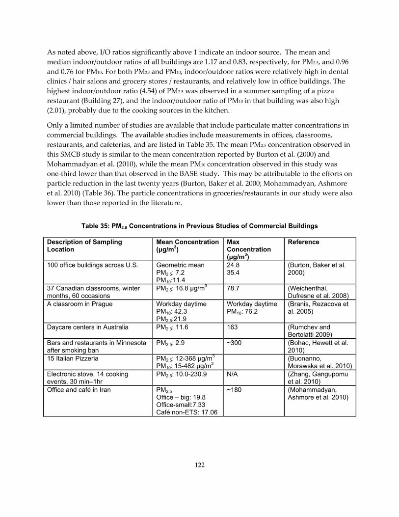
As noted above, I/O ratios significantly above 1 indicate an indoor source.  The mean and median indoor/outdoor ratios of all buildings are 1.17 and 0.83, respectively, for PM2.5, and 0.96 and 0.76 for PM10. For both PM2.5 and PM10, indoor/outdoor ratios were relatively high in dental clinics / hair salons and grocery stores / restaurants, and relatively low in office buildings. The highest indoor/outdoor ratio (4.54) of PM2.5 was observed in a summer sampling of a pizza restaurant (Building 27), and the indoor/outdoor ratio of PM10 in that building was also high (2.01), probably due to the cooking sources in the kitchen. 

Only a limited number of studies are available that include particulate matter concentrations in commercial buildings.  The available studies include measurements in offices, classrooms, restaurants, and cafeterias, and are listed in Table 35. The mean PM2.5 concentration observed in this SMCB study is similar to the mean concentration reported by Burton et al. (2000) and Mohammadyan et al. (2010), while the mean PM10 concentration observed in this study was one‐third lower than that observed in the BASE study.  This may be attributable to the efforts on particle reduction in the last twenty years (Burton, Baker et al. 2000; Mohammadyan, Ashmore et al. 2010) (Table 36). The particle concentrations in groceries/restaurants in our study were also lower than those reported in the literature.  

Table 35: PM2.5 Concentrations in Previous Studies of Commercial Buildings

Description of Sampling Location

Mean Concentration (μg/m3)

Max Concentration (μg/m3)

Reference

100 office buildings across U.S. Geometric mean PM2.5: 7.2 PM10:11.4

24.8 35.4

(Burton, Baker et al. 2000)

37 Canadian classrooms, winter months, 60 occasions

PM2.5: 16.8 μg/m3

78.7 (Weichenthal, Dufresne et al. 2008)

A classroom in Prague Workday daytime PM10: 42.3 PM2.5:21.9

Workday daytime PM10: 76.2

(Branis, Rezacova et al. 2005)

Daycare centers in Australia PM2.5: 11.6 163 (Rumchev and Bertolatti 2009)

Bars and restaurants in Minnesota after smoking ban

PM2.5: 2.9 ~300 (Bohac, Hewett et al. 2010)

15 Italian Pizzeria PM2.5: 12-368 μg/m3 PM10: 15-482 μg/m3

(Buonanno, Morawska et al. 2010)

Electronic stove, 14 cooking events, 30 min–1hr

PM2.5: 10.0-230.9 N/A (Zhang, Gangupomu et al. 2010)

Office and café in Iran PM2.5 Office – big: 19.8 Office-small:7.33 Café non-ETS: 17.06

~180 (Mohammadyan, Ashmore et al. 2010)

 

122 

 

 

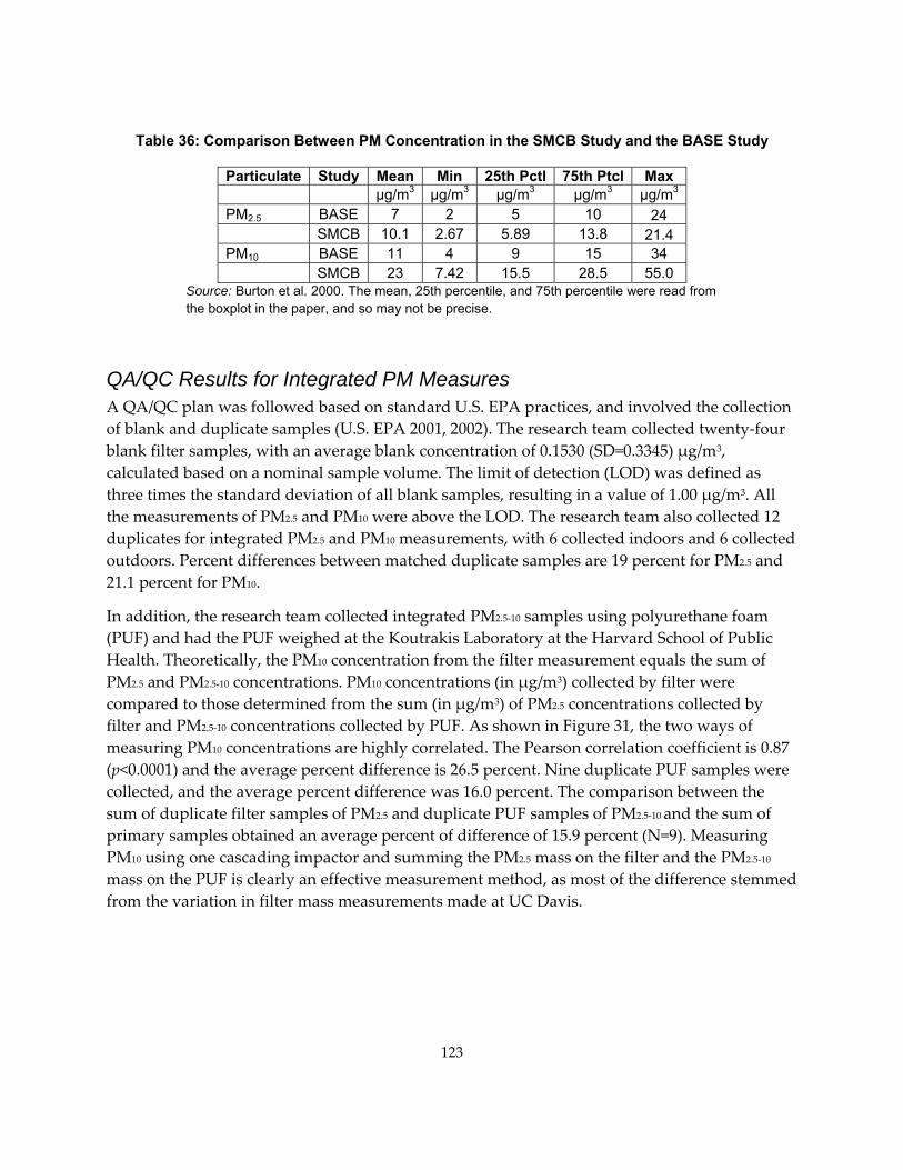
Table 36: Comparison Between PM Concentration in the SMCB Study and the BASE Study

Particulate Study Mean Min 25th Pctl 75th Ptcl Max µg/m3 µg/m3 µg/m3 µg/m3 µg/m3 PM2.5 BASE 7 2 5 10 24 SMCB 10.1 2.67 5.89 13.8 21.4 PM10 BASE 11 4 9 15 34 SMCB 23 7.42 15.5 28.5 55.0

Source: Burton et al. 2000. The mean, 25th percentile, and 75th percentile were read from the boxplot in the paper, and so may not be precise.

 

QA/QC Results for Integrated PM Measures A QA/QC plan was followed based on standard U.S. EPA practices, and involved the collection of blank and duplicate samples (U.S. EPA 2001, 2002). The research team collected twenty‐four blank filter samples, with an average blank concentration of 0.1530 (SD=0.3345) μg/m3, calculated based on a nominal sample volume. The limit of detection (LOD) was defined as three times the standard deviation of all blank samples, resulting in a value of 1.00 μg/m3. All the measurements of PM2.5 and PM10 were above the LOD. The research team also collected 12 duplicates for integrated PM2.5 and PM10 measurements, with 6 collected indoors and 6 collected outdoors. Percent differences between matched duplicate samples are 19 percent for PM2.5 and 21.1 percent for PM10. 

In addition, the research team collected integrated PM2.5‐10 samples using polyurethane foam (PUF) and had the PUF weighed at the Koutrakis Laboratory at the Harvard School of Public Health. Theoretically, the PM10 concentration from the filter measurement equals the sum of PM2.5 and PM2.5‐10 concentrations. PM10 concentrations (in μg/m3) collected by filter were compared to those determined from the sum (in μg/m3) of PM2.5 concentrations collected by filter and PM2.5‐10 concentrations collected by PUF. As shown in Figure 31, the two ways of measuring PM10 concentrations are highly correlated. The Pearson correlation coefficient is 0.87 (p<0.0001) and the average percent difference is 26.5 percent. Nine duplicate PUF samples were collected, and the average percent difference was 16.0 percent. The comparison between the sum of duplicate filter samples of PM2.5 and duplicate PUF samples of PM2.5‐10 and the sum of primary samples obtained an average percent of difference of 15.9 percent (N=9). Measuring PM10 using one cascading impactor and summing the PM2.5 mass on the filter and the PM2.5‐10 mass on the PUF is clearly an effective measurement method, as most of the difference stemmed from the variation in filter mass measurements made at UC Davis.   

123 

 

 

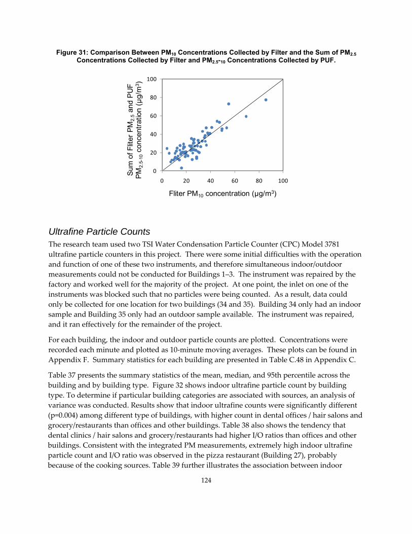
Figure 31: Comparison Between PM10 Concentrations Collected by Filter and the Sum of PM2.5 Concentrations Collected by Filter and PM2.5-10 Concentrations Collected by PUF.

0

20

40

60

80

100

0 20 40 60 80 100

Sum

of F

liter

PM

2.5

and

PUF

PM2.

5-10

conc

entra

tion

(μg/

m3 )

Fliter PM10 concentration (μg/m3) 

 

Ultrafine Particle Counts The research team used two TSI Water Condensation Particle Counter (CPC) Model 3781 ultrafine particle counters in this project.  There were some initial difficulties with the operation and function of one of these two instruments, and therefore simultaneous indoor/outdoor measurements could not be conducted for Buildings 1–3.  The instrument was repaired by the factory and worked well for the majority of the project.  At one point, the inlet on one of the instruments was blocked such that no particles were being counted.  As a result, data could only be collected for one location for two buildings (34 and 35).  Building 34 only had an indoor sample and Building 35 only had an outdoor sample available.  The instrument was repaired, and it ran effectively for the remainder of the project.   

For each building, the indoor and outdoor particle counts are plotted.  Concentrations were recorded each minute and plotted as 10‐minute moving averages.  These plots can be found in Appendix F.  Summary statistics for each building are presented in Table C.48 in Appendix C. 

Table 37 presents the summary statistics of the mean, median, and 95th percentile across the building and by building type.  Figure 32 shows indoor ultrafine particle count by building type. To determine if particular building categories are associated with sources, an analysis of variance was conducted. Results show that indoor ultrafine counts were significantly different (p=0.004) among different type of buildings, with higher count in dental offices / hair salons and grocery/restaurants than offices and other buildings. Table 38 also shows the tendency that dental clinics / hair salons and grocery/restaurants had higher I/O ratios than offices and other buildings. Consistent with the integrated PM measurements, extremely high indoor ultrafine particle count and I/O ratio was observed in the pizza restaurant (Building 27), probably because of the cooking sources. Table 39 further illustrates the association between indoor 

124 

 

 

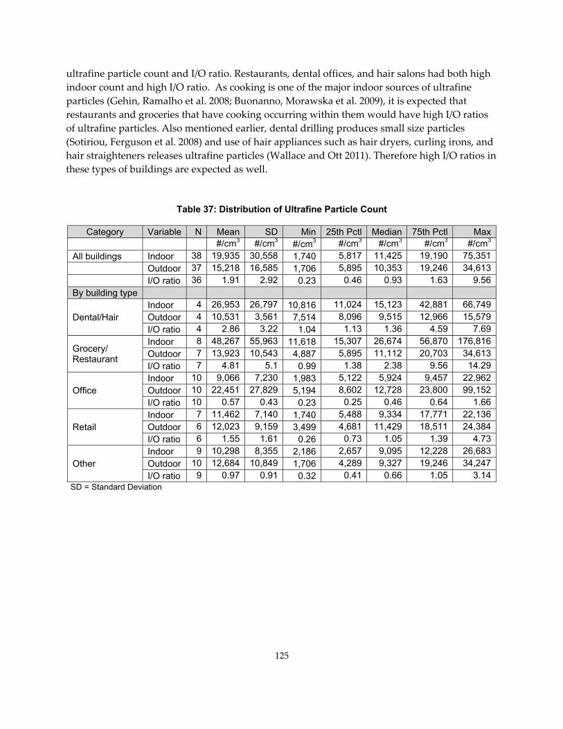
ultrafine particle count and I/O ratio. Restaurants, dental offices, and hair salons had both high indoor count and high I/O ratio.  As cooking is one of the major indoor sources of ultrafine particles (Gehin, Ramalho et al. 2008; Buonanno, Morawska et al. 2009), it is expected that restaurants and groceries that have cooking occurring within them would have high I/O ratios of ultrafine particles. Also mentioned earlier, dental drilling produces small size particles (Sotiriou, Ferguson et al. 2008) and use of hair appliances such as hair dryers, curling irons, and hair straighteners releases ultrafine particles (Wallace and Ott 2011). Therefore high I/O ratios in these types of buildings are expected as well. 

 

Table 37: Distribution of Ultrafine Particle Count

Category Variable N Mean SD Min 25th Pctl Median 75th Pctl Max #/cm3 #/cm3 #/cm3 #/cm3 #/cm3 #/cm3 #/cm3

All buildings Indoor 38 19,935 30,558 1,740 5,817 11,425 19,190 75,351 Outdoor 37 15,218 16,585 1,706 5,895 10,353 19,246 34,613 I/O ratio 36 1.91 2.92 0.23 0.46 0.93 1.63 9.56By building type

Dental/Hair Indoor 4 26,953 26,797 10,816 11,024 15,123 42,881 66,749Outdoor 4 10,531 3,561 7,514 8,096 9,515 12,966 15,579I/O ratio 4 2.86 3.22 1.04 1.13 1.36 4.59 7.69

Grocery/ Restaurant

Indoor 8 48,267 55,963 11,618 15,307 26,674 56,870 176,816Outdoor 7 13,923 10,543 4,887 5,895 11,112 20,703 34,613I/O ratio 7 4.81 5.1 0.99 1.38 2.38 9.56 14.29

Office Indoor 10 9,066 7,230 1,983 5,122 5,924 9,457 22,962Outdoor 10 22,451 27,829 5,194 8,602 12,728 23,800 99,152I/O ratio 10 0.57 0.43 0.23 0.25 0.46 0.64 1.66

Retail Indoor 7 11,462 7,140 1,740 5,488 9,334 17,771 22,136Outdoor 6 12,023 9,159 3,499 4,681 11,429 18,511 24,384I/O ratio 6 1.55 1.61 0.26 0.73 1.05 1.39 4.73

Other Indoor 9 10,298 8,355 2,186 2,657 9,095 12,228 26,683Outdoor 10 12,684 10,849 1,706 4,289 9,327 19,246 34,247I/O ratio 9 0.97 0.91 0.32 0.41 0.66 1.05 3.14

SD = Standard Deviation

125 

 

 

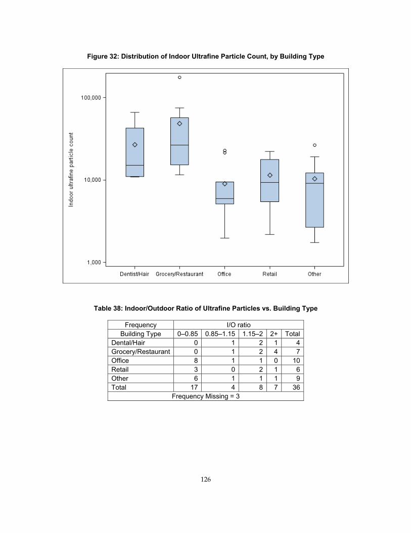
Figure 32: Distribution of Indoor Ultrafine Particle Count, by Building Type 

 

 

Table 38: Indoor/Outdoor Ratio of Ultrafine Particles vs. Building Type  

Frequency I/O ratio Building Type 0–0.85 0.85–1.15 1.15–2 2+ Total

Dental/Hair 0 1 2 1 4 Grocery/Restaurant 0 1 2 4 7 Office 8 1 1 0 10 Retail 3 0 2 1 6 Other 6 1 1 1 9 Total 17 4 8 7 36

Frequency Missing = 3  

126 

 

 

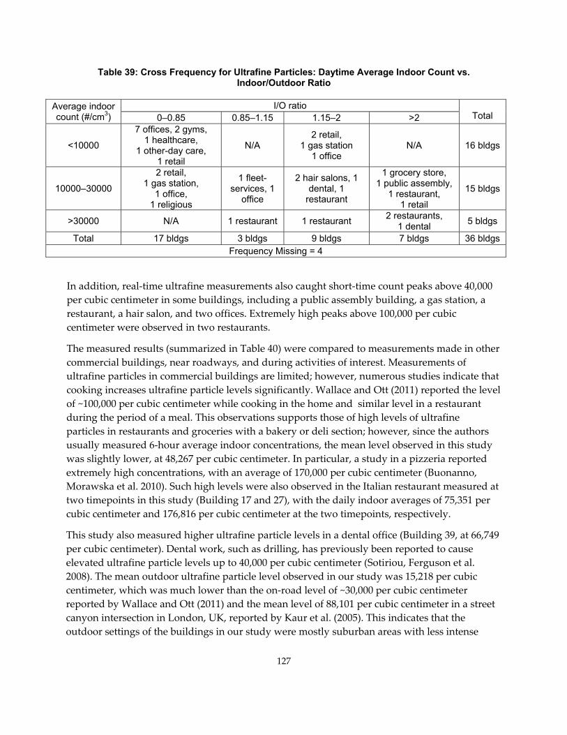
Table 39: Cross Frequency for Ultrafine Particles: Daytime Average Indoor Count vs. Indoor/Outdoor Ratio 

Average indoor count (#/cm3)

I/O ratio Total 0–0.85 0.85–1.15 1.15–2 >2

<10000

7 offices, 2 gyms, 1 healthcare,

1 other-day care, 1 retail

N/A 2 retail,

1 gas station 1 office

N/A 16 bldgs

10000–30000

2 retail, 1 gas station,

1 office, 1 religious

1 fleet-services, 1

office

2 hair salons, 1 dental, 1

restaurant

1 grocery store, 1 public assembly,

1 restaurant, 1 retail

15 bldgs

>30000 N/A 1 restaurant 1 restaurant 2 restaurants, 1 dental 5 bldgs

Total 17 bldgs 3 bldgs 9 bldgs 7 bldgs 36 bldgs Frequency Missing = 4

 

In addition, real‐time ultrafine measurements also caught short‐time count peaks above 40,000 per cubic centimeter in some buildings, including a public assembly building, a gas station, a restaurant, a hair salon, and two offices. Extremely high peaks above 100,000 per cubic centimeter were observed in two restaurants.   

The measured results (summarized in Table 40) were compared to measurements made in other commercial buildings, near roadways, and during activities of interest. Measurements of ultrafine particles in commercial buildings are limited; however, numerous studies indicate that cooking increases ultrafine particle levels significantly. Wallace and Ott (2011) reported the level of ~100,000 per cubic centimeter while cooking in the home and  similar level in a restaurant during the period of a meal. This observations supports those of high levels of ultrafine particles in restaurants and groceries with a bakery or deli section; however, since the authors usually measured 6‐hour average indoor concentrations, the mean level observed in this study was slightly lower, at 48,267 per cubic centimeter. In particular, a study in a pizzeria reported extremely high concentrations, with an average of 170,000 per cubic centimeter (Buonanno, Morawska et al. 2010). Such high levels were also observed in the Italian restaurant measured at two timepoints in this study (Building 17 and 27), with the daily indoor averages of 75,351 per cubic centimeter and 176,816 per cubic centimeter at the two timepoints, respectively.  

This study also measured higher ultrafine particle levels in a dental office (Building 39, at 66,749 per cubic centimeter). Dental work, such as drilling, has previously been reported to cause elevated ultrafine particle levels up to 40,000 per cubic centimeter (Sotiriou, Ferguson et al. 2008). The mean outdoor ultrafine particle level observed in our study was 15,218 per cubic centimeter, which was much lower than the on‐road level of ~30,000 per cubic centimeter reported by Wallace and Ott (2011) and the mean level of 88,101 per cubic centimeter in a street canyon intersection in London, UK, reported by Kaur et al. (2005). This indicates that the outdoor settings of the buildings in our study were mostly suburban areas with less intense 

127 

 

 

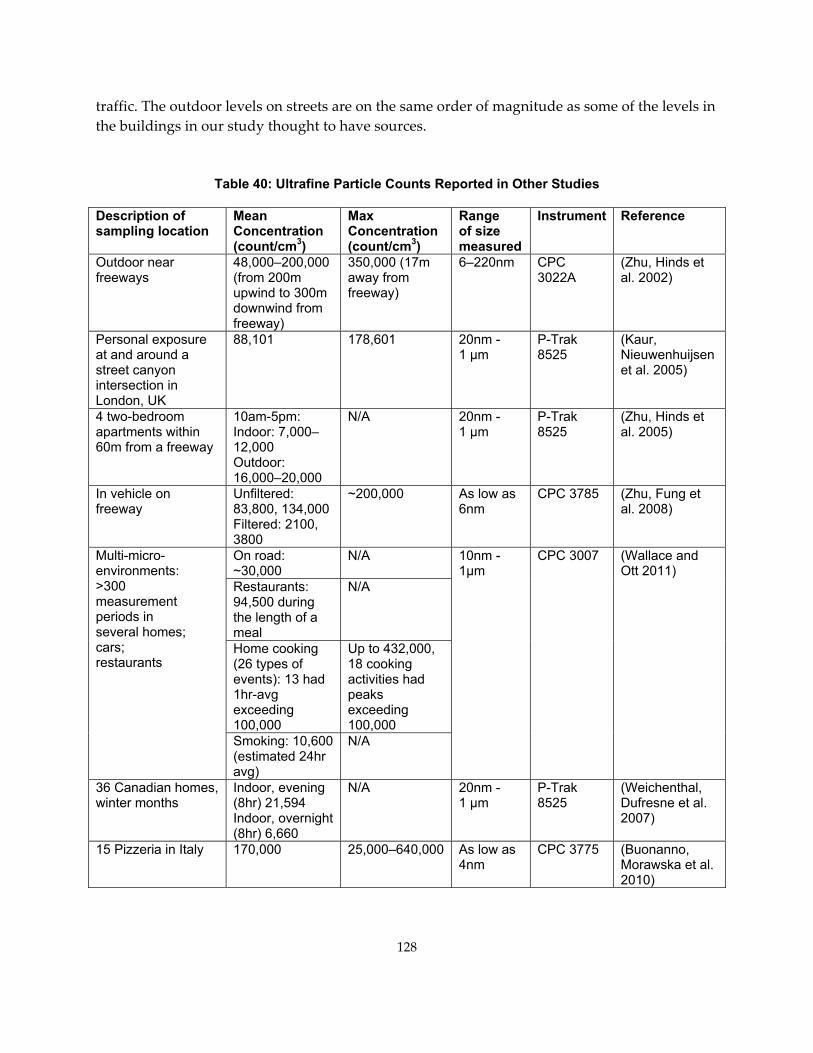
traffic. The outdoor levels on streets are on the same order of magnitude as some of the levels in the buildings in our study thought to have sources.   

 

Table 40: Ultrafine Particle Counts Reported in Other Studies

Description of sampling location

Mean Concentration (count/cm3)

Max Concentration (count/cm3)

Range of size measured

Instrument Reference

Outdoor near freeways

48,000–200,000 (from 200m upwind to 300m downwind from freeway)

350,000 (17m away from freeway)

6–220nm CPC 3022A

(Zhu, Hinds et al. 2002)

Personal exposure at and around a street canyon intersection in London, UK

88,101 178,601 20nm -1 μm

P-Trak 8525

(Kaur, Nieuwenhuijsen et al. 2005)

4 two-bedroom apartments within 60m from a freeway

10am-5pm: Indoor: 7,000–12,000 Outdoor: 16,000–20,000

N/A 20nm -1 μm

P-Trak 8525

(Zhu, Hinds et al. 2005)

In vehicle on freeway

Unfiltered: 83,800, 134,000 Filtered: 2100, 3800

~200,000 As low as 6nm

CPC 3785 (Zhu, Fung et al. 2008)

Multi-micro-environments: >300 measurement periods in several homes; cars; restaurants

On road: ~30,000

N/A 10nm - 1μm

CPC 3007 (Wallace and Ott 2011)

Restaurants: 94,500 during the length of a meal

N/A

Home cooking (26 types of events): 13 had 1hr-avg exceeding 100,000

Up to 432,000, 18 cooking activities had peaks exceeding 100,000

Smoking: 10,600 (estimated 24hr avg)

N/A

36 Canadian homes, winter months

Indoor, evening (8hr) 21,594 Indoor, overnight (8hr) 6,660

N/A 20nm -1 μm

P-Trak 8525

(Weichenthal, Dufresne et al. 2007)

15 Pizzeria in Italy 170,000 25,000–640,000 As low as 4nm

CPC 3775 (Buonanno, Morawska et al. 2010)

128 

 

 

 

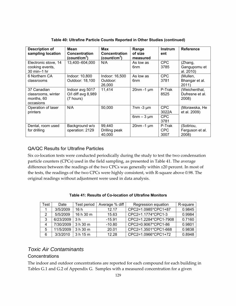
Table 40: Ultrafine Particle Counts Reported in Other Studies (continued)

Description of sampling location

Mean Concentration (count/cm3)

Max Concentration (count/cm3)

Range of size measured

Instrument

Reference

Electronic stove, 14 cooking events, 30 min–1 hr

13,400–604,000 N/A As low as 6nm

CPC 3785

(Zhang, Gangupomu et al. 2010)

6 Northern CA classrooms

Indoor: 10,800 Outdoor: 18,100

Indoor: 16,500 Outdoor: 26,000

As low as 6nm

CPC 3781

(Mullen, Bhangar et al. 2011)

37 Canadian classrooms, winter months, 60 occasions

Indoor avg 5017 O/I diff avg 8,989 (7 hours)

11,414 20nm -1 μm P-Trak 8525

(Weichenthal, Dufresne et al. 2008)

Operation of laser printers

N/A 50,000 7nm -3 μm CPC 3022A

(Morawska, He et al. 2009)

6nm – 3 μm CPC 3781

Dental, room used for drilling

Background w/o operation: 2129

99,440 Drilling peak 40,000

20nm -1 μm P-Trak CPC 3007

(Sotiriou, Ferguson et al. 2008)

 

QA/QC Results for Ultrafine Particles Six co‐location tests were conducted periodically during the study to test the two condensation particle counters (CPCs) used in the field sampling, as presented in Table 41. The average difference between the readings of the two CPCs was generally within ±20 percent. In most of the tests, the readings of the two CPCs were highly consistent, with R‐square above 0.98. The original readings without adjustment were used in data analysis. 

 

Table 41: Results of Co-location of Ultrafine Monitors 

Test Date Test period Average % diff Regression equation R-square1 3/5/2009 16 h 12.17 CPC2=1.0985*CPC1+87 0.98452 5/5/2009 16 h 30 m 15.63 CPC2=1.1774*CPC1-3 0.99843 6/23/2009 3 h -15.91 CPC2=1.2284*CPC1-7908 0.71604 7/30/2009 3 h 30 m -10.80 CPC2=0.9067*CPC1-86 0.98015 11/5/2009 3 h 30 m 20.01 CPC2=1.3501*CPC1-668 0.98386 3/3/2010 3 h 15 m 12.28 CPC2=1.0966*CPC1+72 0.8948

 

Toxic Air Contaminants Concentrations The indoor and outdoor concentrations are reported for each compound for each building in Tables G.1 and G.2 of Appendix G.  Samples with a measured concentration for a given 

129 

 

 

compound under the method detection limit (MDL), which is the lowest concentration level that can be determined to be statistically different from a blank at a 99 percent confidence level, are indicated as non‐detectable concentrations and are replaced with a half MDL for that compound when calculating summary statistics.  The MDL is estimated from the standard deviation of seven replicate analyses of field blanks, and represents the  99 percent confidence level that the measured concentration exceeds zero.  The mass was reported from the laboratory if it was greater than the MDL, even if it was below the analytical Limit of Quantification (LOQ).  The LOQ is mathematically defined as equal to 10 times the standard deviation of the replicate analyses used to determine MDL. If a sample is below the analytical LOQ, it is noted in Tables G.1 and G.2 in Appendix G.   

The VOC sample volume was 5 liters for the pilot study.  In some cases, the amount of chemical was above the quantification range, indicating that the sample volume was too high.  These extreme values are of interest and should be accurately quantified, as they potentially reflect conditions in the buildings with the highest levels of exposure.  On the other extreme, many compounds were below the MDL, particularly outdoors.  For these reasons, the research team used sample volumes of 4 L indoors and 10 L outdoors for the main study.  In a limited number of cases, a lower sample volume was used, as we were concerned that levels would be very high in the building and did not want to exceed the quantification range.  Specifically, 2 L were collected in Buildings 10, 29, and 35.  In some cases, 4 L were inadvertently collected for the outdoor sample. All the concentrations were calculated based on the real volume collected during the sampling. 

When maximum values are exceeded, the values are listed as above quantification range (AQR).  For D5‐siloxane, concentrations above the quantitative range were observed in 13 indoor samples. Since concentration of this compound was rarely reported in the literature before, to retain maximum information, the investigators decided to code those observations as values slightly above quantitative limit (120–127 vs. AQR at 117.03) in further statistical analysis. These assigned numbers should be considered to be a low estimate of actual values. 

During June 2009, samples were contaminated with methylene chloride and n‐hexane while being stored in the freezer.  Only a portion of the samples appear to have been affected, as duplicate pairs had significantly different levels in some cases.  The lower of the two concentrations was used in analysis from the duplicate pairs. For accuracy, the authors excluded all methylene chloride data collected during this period from further statistical analysis, as noted in Table 42.  There were two other instances (one outdoor sample from Building 32 and one indoor sample from Building 34) in which the analysis of the actual sample appeared to have failed, as all concentrations were non‐detectable. This situation most likely happened because the sample did not properly load into the thermal desorption system of the gas chromatograph.  In these cases, concentrations from the duplicate tube were used. 

130 

 

 

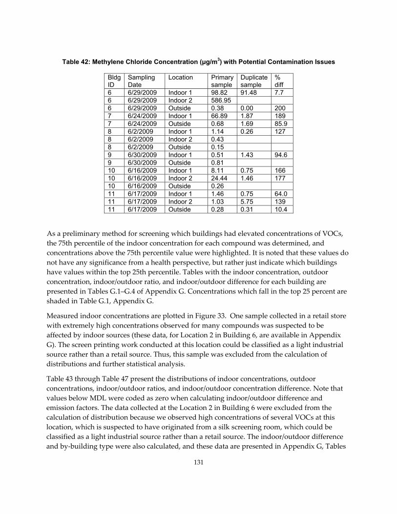
Table 42: Methylene Chloride Concentration (μg/m3) with Potential Contamination Issues

Bldg ID

Sampling Date

Location Primary sample

Duplicate sample

% diff

6 6/29/2009 Indoor 1 98.82 91.48 7.7 6 6/29/2009 Indoor 2 586.95 6 6/29/2009 Outside 0.38 0.00 200 7 6/24/2009 Indoor 1 66.89 1.87 189 7 6/24/2009 Outside 0.68 1.69 85.9 8 6/2/2009 Indoor 1 1.14 0.26 127 8 6/2/2009 Indoor 2 0.43 8 6/2/2009 Outside 0.15 9 6/30/2009 Indoor 1 0.51 1.43 94.6 9 6/30/2009 Outside 0.81 10 6/16/2009 Indoor 1 8.11 0.75 166 10 6/16/2009 Indoor 2 24.44 1.46 177 10 6/16/2009 Outside 0.26 11 6/17/2009 Indoor 1 1.46 0.75 64.0 11 6/17/2009 Indoor 2 1.03 5.75 139 11 6/17/2009 Outside 0.28 0.31 10.4

 

As a preliminary method for screening which buildings had elevated concentrations of VOCs, the 75th percentile of the indoor concentration for each compound was determined, and concentrations above the 75th percentile value were highlighted. It is noted that these values do not have any significance from a health perspective, but rather just indicate which buildings have values within the top 25th percentile. Tables with the indoor concentration, outdoor concentration, indoor/outdoor ratio, and indoor/outdoor difference for each building are presented in Tables G.1–G.4 of Appendix G. Concentrations which fall in the top 25 percent are shaded in Table G.1, Appendix G. 

Measured indoor concentrations are plotted in Figure 33.  One sample collected in a retail store with extremely high concentrations observed for many compounds was suspected to be affected by indoor sources (these data, for Location 2 in Building 6, are available in Appendix G). The screen printing work conducted at this location could be classified as a light industrial source rather than a retail source. Thus, this sample was excluded from the calculation of distributions and further statistical analysis.  

Table 43 through Table 47 present the distributions of indoor concentrations, outdoor concentrations, indoor/outdoor ratios, and indoor/outdoor concentration difference. Note that values below MDL were coded as zero when calculating indoor/outdoor difference and emission factors. The data collected at the Location 2 in Building 6 were excluded from the calculation of distribution because we observed high concentrations of several VOCs at this location, which is suspected to have originated from a silk screening room, which could be classified as a light industrial source rather than a retail source. The indoor/outdoor difference and by‐building type were also calculated, and these data are presented in Appendix G, Tables 

131 

 

 

G.5‐G.11. Extremely high concentrations of some VOCs, which were higher than five times the standard deviation, were observed in some buildings. The values are listed in Table 48Table , along with the possible causes or sources and are included in the distributions presented in Tables 43–47, with the exception of Location 2 in Building 6, as noted above.  In one building, the suspected source was indoor smoking, which theoretically should not be a source inside workplaces in California.  The field staff was not at the office during lunchtime, and the ultrafine monitor indicated high concentrations during the lunch hour.  This, coupled with the fact that the indoor benzene concentrations were higher than the outdoor benzene concentrations, noting that there are very few known indoor sources of benzene, along with the attitude of the employees at the building, led the researchers to suspect that smoking had occurred during lunch. 

132 

 

 

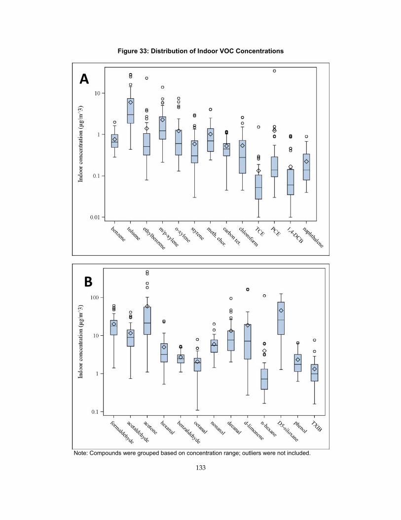
Figure 33: Distribution of Indoor VOC Concentrations

 

A 

 

B 

Note: Compounds were grouped based on concentration range; outliers were not included.

133 

 

 

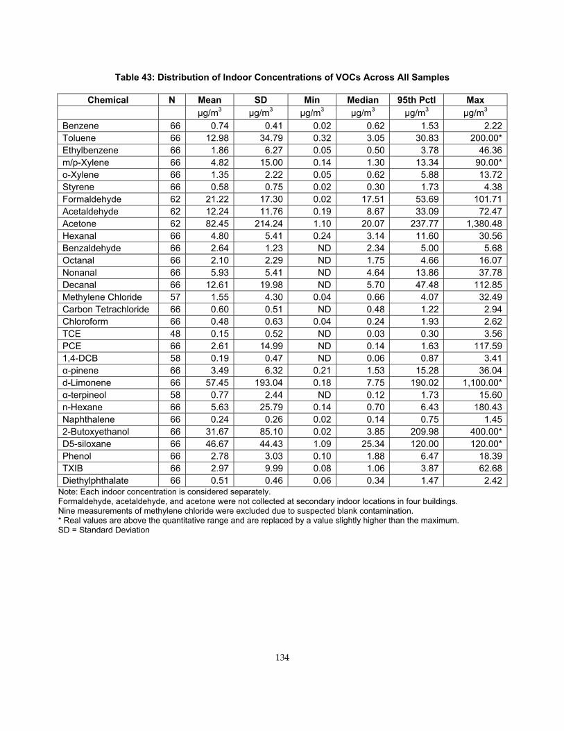
Table 43: Distribution of Indoor Concentrations of VOCs Across All Samples

Chemical N Mean SD Min Median 95th Pctl Max µg/m3 µg/m3 µg/m3 µg/m3 µg/m3 µg/m3

Benzene 66 0.74 0.41 0.02 0.62 1.53 2.22Toluene 66 12.98 34.79 0.32 3.05 30.83 200.00*Ethylbenzene 66 1.86 6.27 0.05 0.50 3.78 46.36m/p-Xylene 66 4.82 15.00 0.14 1.30 13.34 90.00*o-Xylene 66 1.35 2.22 0.05 0.62 5.88 13.72Styrene 66 0.58 0.75 0.02 0.30 1.73 4.38Formaldehyde 62 21.22 17.30 0.02 17.51 53.69 101.71Acetaldehyde 62 12.24 11.76 0.19 8.67 33.09 72.47Acetone 62 82.45 214.24 1.10 20.07 237.77 1,380.48Hexanal 66 4.80 5.41 0.24 3.14 11.60 30.56Benzaldehyde 66 2.64 1.23 ND 2.34 5.00 5.68Octanal 66 2.10 2.29 ND 1.75 4.66 16.07Nonanal 66 5.93 5.41 ND 4.64 13.86 37.78Decanal 66 12.61 19.98 ND 5.70 47.48 112.85Methylene Chloride 57 1.55 4.30 0.04 0.66 4.07 32.49Carbon Tetrachloride 66 0.60 0.51 ND 0.48 1.22 2.94Chloroform 66 0.48 0.63 0.04 0.24 1.93 2.62TCE 48 0.15 0.52 ND 0.03 0.30 3.56PCE 66 2.61 14.99 ND 0.14 1.63 117.591,4-DCB 58 0.19 0.47 ND 0.06 0.87 3.41α-pinene 66 3.49 6.32 0.21 1.53 15.28 36.04d-Limonene 66 57.45 193.04 0.18 7.75 190.02 1,100.00*α-terpineol 58 0.77 2.44 ND 0.12 1.73 15.60n-Hexane 66 5.63 25.79 0.14 0.70 6.43 180.43Naphthalene 66 0.24 0.26 0.02 0.14 0.75 1.452-Butoxyethanol 66 31.67 85.10 0.02 3.85 209.98 400.00*D5-siloxane 66 46.67 44.43 1.09 25.34 120.00 120.00*Phenol 66 2.78 3.03 0.10 1.88 6.47 18.39TXIB 66 2.97 9.99 0.08 1.06 3.87 62.68Diethylphthalate 66 0.51 0.46 0.06 0.34 1.47 2.42

Note: Each indoor concentration is considered separately. Formaldehyde, acetaldehyde, and acetone were not collected at secondary indoor locations in four buildings. Nine measurements of methylene chloride were excluded due to suspected blank contamination. * Real values are above the quantitative range and are replaced by a value slightly higher than the maximum. SD = Standard Deviation

134 

 

 

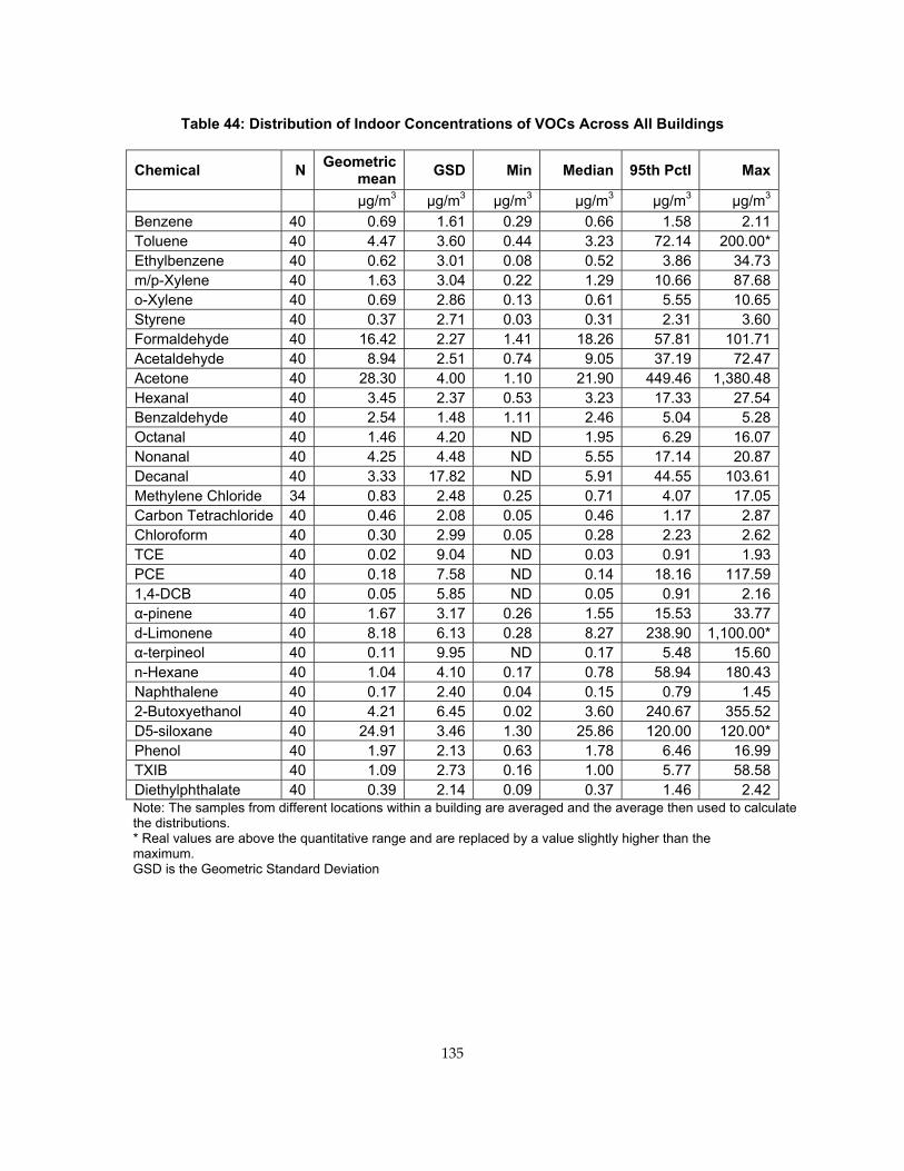
Table 44: Distribution of Indoor Concentrations of VOCs Across All Buildings

Chemical N Geometric mean GSD Min Median 95th Pctl Max

µg/m3 µg/m3 µg/m3 µg/m3 µg/m3 µg/m3

Benzene 40 0.69 1.61 0.29 0.66 1.58 2.11Toluene 40 4.47 3.60 0.44 3.23 72.14 200.00*Ethylbenzene 40 0.62 3.01 0.08 0.52 3.86 34.73m/p-Xylene 40 1.63 3.04 0.22 1.29 10.66 87.68o-Xylene 40 0.69 2.86 0.13 0.61 5.55 10.65Styrene 40 0.37 2.71 0.03 0.31 2.31 3.60Formaldehyde 40 16.42 2.27 1.41 18.26 57.81 101.71Acetaldehyde 40 8.94 2.51 0.74 9.05 37.19 72.47Acetone 40 28.30 4.00 1.10 21.90 449.46 1,380.48Hexanal 40 3.45 2.37 0.53 3.23 17.33 27.54Benzaldehyde 40 2.54 1.48 1.11 2.46 5.04 5.28Octanal 40 1.46 4.20 ND 1.95 6.29 16.07Nonanal 40 4.25 4.48 ND 5.55 17.14 20.87Decanal 40 3.33 17.82 ND 5.91 44.55 103.61Methylene Chloride 34 0.83 2.48 0.25 0.71 4.07 17.05Carbon Tetrachloride 40 0.46 2.08 0.05 0.46 1.17 2.87Chloroform 40 0.30 2.99 0.05 0.28 2.23 2.62TCE 40 0.02 9.04 ND 0.03 0.91 1.93PCE 40 0.18 7.58 ND 0.14 18.16 117.591,4-DCB 40 0.05 5.85 ND 0.05 0.91 2.16α-pinene 40 1.67 3.17 0.26 1.55 15.53 33.77d-Limonene 40 8.18 6.13 0.28 8.27 238.90 1,100.00*α-terpineol 40 0.11 9.95 ND 0.17 5.48 15.60n-Hexane 40 1.04 4.10 0.17 0.78 58.94 180.43Naphthalene 40 0.17 2.40 0.04 0.15 0.79 1.452-Butoxyethanol 40 4.21 6.45 0.02 3.60 240.67 355.52D5-siloxane 40 24.91 3.46 1.30 25.86 120.00 120.00*Phenol 40 1.97 2.13 0.63 1.78 6.46 16.99TXIB 40 1.09 2.73 0.16 1.00 5.77 58.58Diethylphthalate 40 0.39 2.14 0.09 0.37 1.46 2.42Note: The samples from different locations within a building are averaged and the average then used to calculate the distributions. * Real values are above the quantitative range and are replaced by a value slightly higher than the maximum. GSD is the Geometric Standard Deviation

135 

 

 

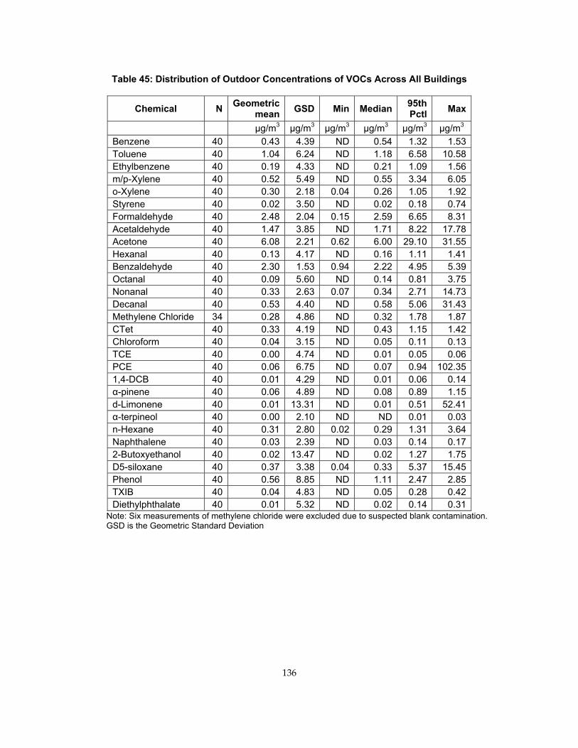
Table 45: Distribution of Outdoor Concentrations of VOCs Across All Buildings 

Chemical N Geometric mean GSD Min Median 95th

Pctl Max

µg/m3 µg/m3 µg/m3 µg/m3 µg/m3 µg/m3 Benzene 40 0.43 4.39 ND 0.54 1.32 1.53Toluene 40 1.04 6.24 ND 1.18 6.58 10.58Ethylbenzene 40 0.19 4.33 ND 0.21 1.09 1.56m/p-Xylene 40 0.52 5.49 ND 0.55 3.34 6.05o-Xylene 40 0.30 2.18 0.04 0.26 1.05 1.92Styrene 40 0.02 3.50 ND 0.02 0.18 0.74Formaldehyde 40 2.48 2.04 0.15 2.59 6.65 8.31Acetaldehyde 40 1.47 3.85 ND 1.71 8.22 17.78Acetone 40 6.08 2.21 0.62 6.00 29.10 31.55Hexanal 40 0.13 4.17 ND 0.16 1.11 1.41Benzaldehyde 40 2.30 1.53 0.94 2.22 4.95 5.39Octanal 40 0.09 5.60 ND 0.14 0.81 3.75Nonanal 40 0.33 2.63 0.07 0.34 2.71 14.73Decanal 40 0.53 4.40 ND 0.58 5.06 31.43Methylene Chloride 34 0.28 4.86 ND 0.32 1.78 1.87CTet 40 0.33 4.19 ND 0.43 1.15 1.42Chloroform 40 0.04 3.15 ND 0.05 0.11 0.13TCE 40 0.00 4.74 ND 0.01 0.05 0.06PCE 40 0.06 6.75 ND 0.07 0.94 102.351,4-DCB 40 0.01 4.29 ND 0.01 0.06 0.14α-pinene 40 0.06 4.89 ND 0.08 0.89 1.15d-Limonene 40 0.01 13.31 ND 0.01 0.51 52.41α-terpineol 40 0.00 2.10 ND ND 0.01 0.03n-Hexane 40 0.31 2.80 0.02 0.29 1.31 3.64Naphthalene 40 0.03 2.39 ND 0.03 0.14 0.172-Butoxyethanol 40 0.02 13.47 ND 0.02 1.27 1.75D5-siloxane 40 0.37 3.38 0.04 0.33 5.37 15.45Phenol 40 0.56 8.85 ND 1.11 2.47 2.85TXIB 40 0.04 4.83 ND 0.05 0.28 0.42Diethylphthalate 40 0.01 5.32 ND 0.02 0.14 0.31

Note: Six measurements of methylene chloride were excluded due to suspected blank contamination. GSD is the Geometric Standard Deviation 

 

 

 

 

 

136 

 

 

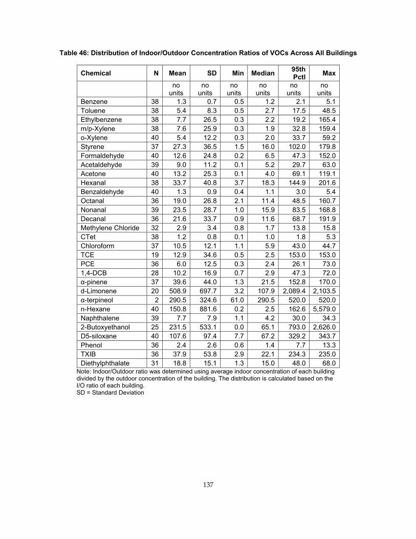
Table 46: Distribution of Indoor/Outdoor Concentration Ratios of VOCs Across All Buildings

Chemical N Mean SD Min Median 95th Pctl Max

no units

no units

no units

no units

no units

no units

Benzene 38 1.3 0.7 0.5 1.2 2.1 5.1Toluene 38 5.4 8.3 0.5 2.7 17.5 48.5Ethylbenzene 38 7.7 26.5 0.3 2.2 19.2 165.4m/p-Xylene 38 7.6 25.9 0.3 1.9 32.8 159.4o-Xylene 40 5.4 12.2 0.3 2.0 33.7 59.2Styrene 37 27.3 36.5 1.5 16.0 102.0 179.8Formaldehyde 40 12.6 24.8 0.2 6.5 47.3 152.0Acetaldehyde 39 9.0 11.2 0.1 5.2 29.7 63.0Acetone 40 13.2 25.3 0.1 4.0 69.1 119.1Hexanal 38 33.7 40.8 3.7 18.3 144.9 201.6Benzaldehyde 40 1.3 0.9 0.4 1.1 3.0 5.4Octanal 36 19.0 26.8 2.1 11.4 48.5 160.7Nonanal 39 23.5 28.7 1.0 15.9 83.5 168.8Decanal 36 21.6 33.7 0.9 11.6 68.7 191.9Methylene Chloride 32 2.9 3.4 0.8 1.7 13.8 15.8CTet 38 1.2 0.8 0.1 1.0 1.8 5.3Chloroform 37 10.5 12.1 1.1 5.9 43.0 44.7TCE 19 12.9 34.6 0.5 2.5 153.0 153.0PCE 36 6.0 12.5 0.3 2.4 26.1 73.01,4-DCB 28 10.2 16.9 0.7 2.9 47.3 72.0α-pinene 37 39.6 44.0 1.3 21.5 152.8 170.0d-Limonene 20 508.9 697.7 3.2 107.9 2,089.4 2,103.5α-terpineol 2 290.5 324.6 61.0 290.5 520.0 520.0n-Hexane 40 150.8 881.6 0.2 2.5 162.6 5,579.0Naphthalene 39 7.7 7.9 1.1 4.2 30.0 34.32-Butoxyethanol 25 231.5 533.1 0.0 65.1 793.0 2,626.0D5-siloxane 40 107.6 97.4 7.7 67.2 329.2 343.7Phenol 36 2.4 2.6 0.6 1.4 7.7 13.3TXIB 36 37.9 53.8 2.9 22.1 234.3 235.0Diethylphthalate 31 18.8 15.1 1.3 15.0 48.0 68.0

Note: Indoor/Outdoor ratio was determined using average indoor concentration of each building divided by the outdoor concentration of the building. The distribution is calculated based on the I/O ratio of each building. SD = Standard Deviation

 

 

 

 

 

137 

 

 

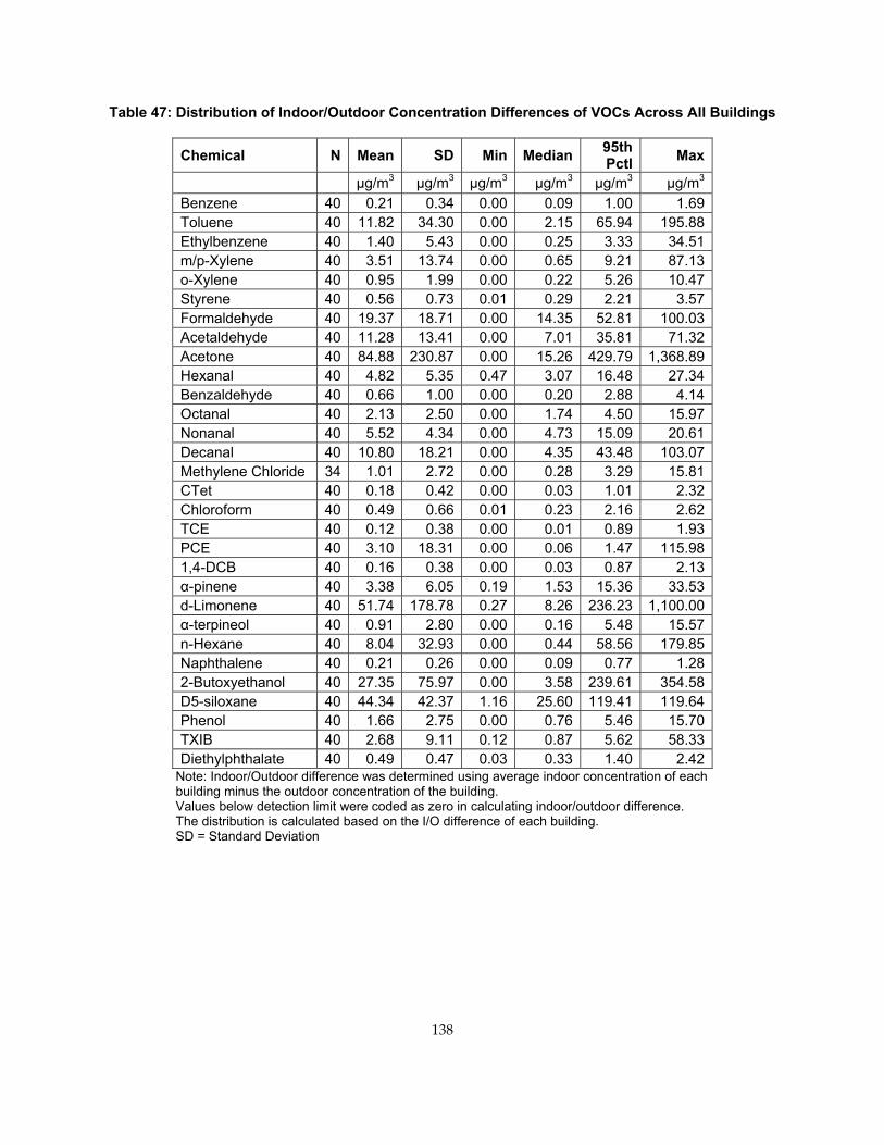
Table 47: Distribution of Indoor/Outdoor Concentration Differences of VOCs Across All Buildings  

Chemical N Mean SD Min Median 95th Pctl Max

µg/m3 µg/m3 µg/m3 µg/m3 µg/m3 µg/m3 Benzene 40 0.21 0.34 0.00 0.09 1.00 1.69 Toluene 40 11.82 34.30 0.00 2.15 65.94 195.88 Ethylbenzene 40 1.40 5.43 0.00 0.25 3.33 34.51 m/p-Xylene 40 3.51 13.74 0.00 0.65 9.21 87.13 o-Xylene 40 0.95 1.99 0.00 0.22 5.26 10.47 Styrene 40 0.56 0.73 0.01 0.29 2.21 3.57 Formaldehyde 40 19.37 18.71 0.00 14.35 52.81 100.03 Acetaldehyde 40 11.28 13.41 0.00 7.01 35.81 71.32 Acetone 40 84.88 230.87 0.00 15.26 429.79 1,368.89 Hexanal 40 4.82 5.35 0.47 3.07 16.48 27.34 Benzaldehyde 40 0.66 1.00 0.00 0.20 2.88 4.14 Octanal 40 2.13 2.50 0.00 1.74 4.50 15.97 Nonanal 40 5.52 4.34 0.00 4.73 15.09 20.61 Decanal 40 10.80 18.21 0.00 4.35 43.48 103.07 Methylene Chloride 34 1.01 2.72 0.00 0.28 3.29 15.81 CTet 40 0.18 0.42 0.00 0.03 1.01 2.32 Chloroform 40 0.49 0.66 0.01 0.23 2.16 2.62 TCE 40 0.12 0.38 0.00 0.01 0.89 1.93 PCE 40 3.10 18.31 0.00 0.06 1.47 115.98 1,4-DCB 40 0.16 0.38 0.00 0.03 0.87 2.13 α-pinene 40 3.38 6.05 0.19 1.53 15.36 33.53 d-Limonene 40 51.74 178.78 0.27 8.26 236.23 1,100.00 α-terpineol 40 0.91 2.80 0.00 0.16 5.48 15.57 n-Hexane 40 8.04 32.93 0.00 0.44 58.56 179.85 Naphthalene 40 0.21 0.26 0.00 0.09 0.77 1.28 2-Butoxyethanol 40 27.35 75.97 0.00 3.58 239.61 354.58 D5-siloxane 40 44.34 42.37 1.16 25.60 119.41 119.64 Phenol 40 1.66 2.75 0.00 0.76 5.46 15.70 TXIB 40 2.68 9.11 0.12 0.87 5.62 58.33 Diethylphthalate 40 0.49 0.47 0.03 0.33 1.40 2.42

Note: Indoor/Outdoor difference was determined using average indoor concentration of each building minus the outdoor concentration of the building. Values below detection limit were coded as zero in calculating indoor/outdoor difference. The distribution is calculated based on the I/O difference of each building. SD = Standard Deviation

      

138 

 

 

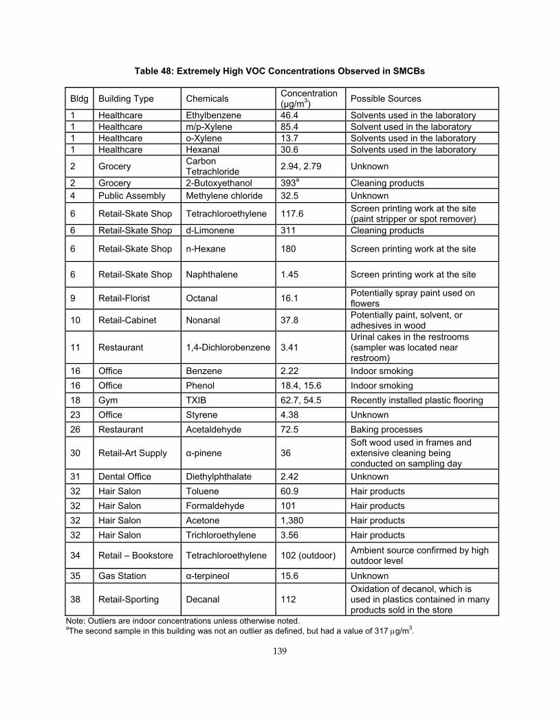
Table 48: Extremely High VOC Concentrations Observed in SMCBs

Bldg Building Type Chemicals Concentration (µg/m3) Possible Sources

1 Healthcare Ethylbenzene 46.4 Solvents used in the laboratory 1 Healthcare m/p-Xylene 85.4 Solvent used in the laboratory 1 Healthcare o-Xylene 13.7 Solvents used in the laboratory 1 Healthcare Hexanal 30.6 Solvents used in the laboratory

2 Grocery Carbon Tetrachloride 2.94, 2.79 Unknown

2 Grocery 2-Butoxyethanol 393a Cleaning products 4 Public Assembly Methylene chloride 32.5 Unknown

6 Retail-Skate Shop Tetrachloroethylene 117.6 Screen printing work at the site (paint stripper or spot remover)

6 Retail-Skate Shop d-Limonene 311 Cleaning products

6 Retail-Skate Shop n-Hexane 180 Screen printing work at the site

6 Retail-Skate Shop Naphthalene 1.45 Screen printing work at the site

9 Retail-Florist Octanal 16.1 Potentially spray paint used on flowers

10 Retail-Cabinet Nonanal 37.8 Potentially paint, solvent, or adhesives in wood

11 Restaurant 1,4-Dichlorobenzene 3.41 Urinal cakes in the restrooms (sampler was located near restroom)

16 Office Benzene 2.22 Indoor smoking 16 Office Phenol 18.4, 15.6 Indoor smoking 18 Gym TXIB 62.7, 54.5 Recently installed plastic flooring 23 Office Styrene 4.38 Unknown 26 Restaurant Acetaldehyde 72.5 Baking processes

30 Retail-Art Supply α-pinene 36 Soft wood used in frames and extensive cleaning being conducted on sampling day

31 Dental Office Diethylphthalate 2.42 Unknown 32 Hair Salon Toluene 60.9 Hair products 32 Hair Salon Formaldehyde 101 Hair products 32 Hair Salon Acetone 1,380 Hair products 32 Hair Salon Trichloroethylene 3.56 Hair products

34 Retail – Bookstore Tetrachloroethylene 102 (outdoor) Ambient source confirmed by high outdoor level

35 Gas Station α-terpineol 15.6 Unknown

38 Retail-Sporting Decanal 112 Oxidation of decanol, which is used in plastics contained in many products sold in the store

Note: Outliers are indoor concentrations unless otherwise noted. aThe second sample in this building was not an outlier as defined, but had a value of 317 μg/m3. 

139 

 

 

 

The authors compared indoor VOC concentrations by building use, and statistically significant differences (p<0.05) were observed for ethylbenzene, o‐xylene, chloroform, PCE, naphthalene, phenol, TXIB, and diethylphthalate (DEP). Concentrations of benzene, m/p‐xylene, acetaldehyde, octanal, and D5‐siloxane were marginally different (p=0.05–0.09) by building type. Indoor concentrations of these compounds by building type are presented in Figures 34 through 47. 

Phenol, DEP and D5‐siloxane are used in personal care products, and higher concentrations of these compounds were found in buildings with use of personal care products or with higher occupant density (Figures 34–36 ). The concentrations of D5‐siloxane were significantly higher in hair salons/gyms and dental offices/healthcare facilities, which might use more products containing D5‐siloxane than in buildings with other uses. D5‐siloxane was also sometimes above quantitative range in offices and groceries/restaurants, possibly due to high occupant density in the buildings.  Phenol was used in the manufacture of resins and nylon but also used in cosmetics, e.g., sunscreen and hair dyes and as a disinfectant and antiseptic. The concentrations were significantly higher in offices than in other types of buildings. Diethylphthalate was higher in hair salons/gym and dental office/healthcare facilities than in buildings with other uses. 

High concentrations of ethylbenzene, m/p‐xylene, and o‐xylene were observed in a medium‐sized healthcare building, and it is possible that these chemicals were used as solvents in the laboratory in this building (Figures 37–39). Except in the case of the healthcare building, these three compounds had relatively higher concentrations in fleet service offices / gas station convenience stores and retailers. Groceries/restaurants and miscellaneous buildings had low levels of these compounds. Concentrations of benzene were high in a fleet service building and gas station convenience stores (Figure 40), probably the result of gasoline evaporation. Concentrations above 2 μg/m3 were observed in the retail store with screen printing and in an office with suspected smoking behavior. 

Acetaldehyde occurs naturally in some foods such as ripe fruits and is also a byproduct of yeast used in baking. It was significantly higher in groceries/restaurants than other types of buildings, with concentrations up to 72.5 μg/m3 (Figure 41). Concentrations of chloroform were also significantly high in groceries/restaurants (Figure 42), and may be due to volatilization from the large amount of tap water that was used for cleaning and cooking. 

While PCE was statistically significantly higher in retail stores, the authors do not consider this result generalizable, as two retail stores had extremely high concentrations of PCE, one being in the retail space of the retail store that included screen printing (which may have used PCE), and the second being in a bookstore with a high outdoor concentration measured on site (Figure 43).  

Naphthalene has been used as a fumigant, and the concentrations were high in some of the retail stores and low in groceries/restaurants and miscellaneous buildings (Figure 44). Octanal concentrations were also found to be higher in retail stores. 

140 

 

 

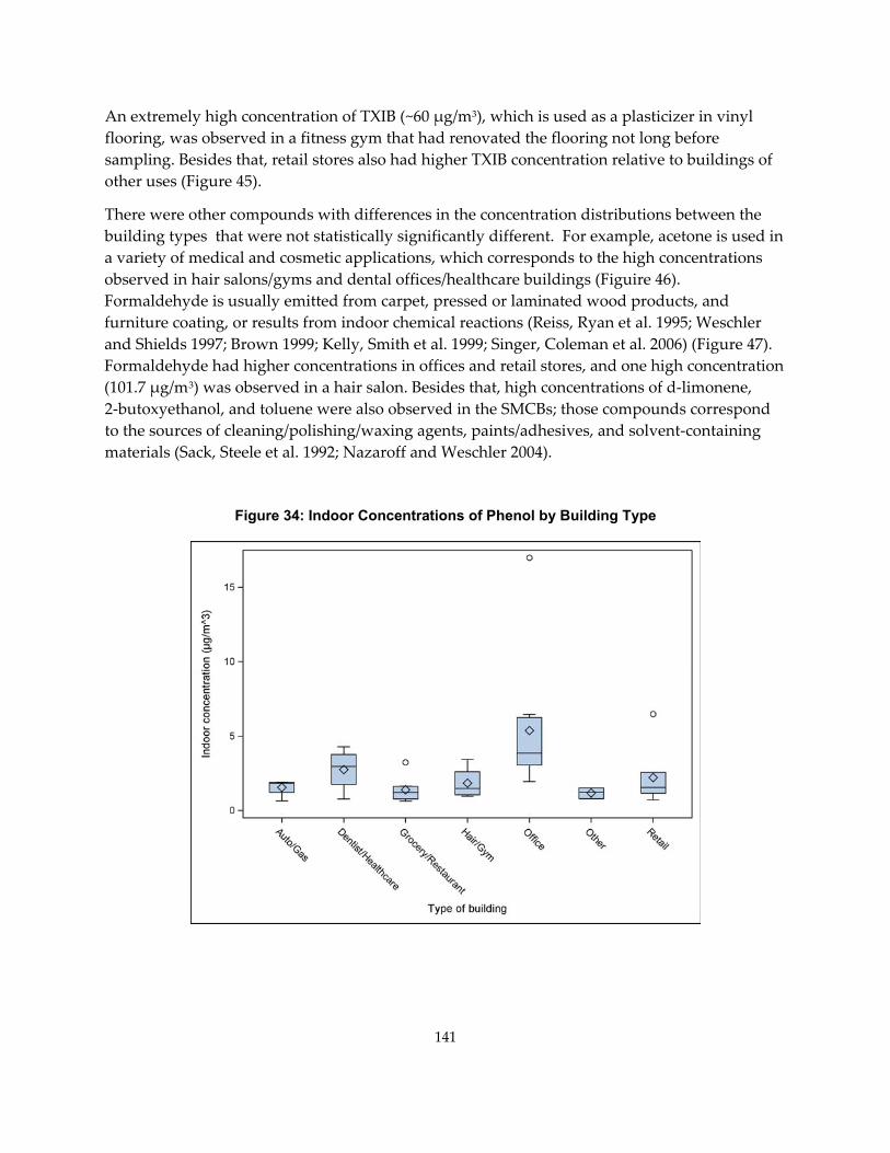
An extremely high concentration of TXIB (~60 μg/m3), which is used as a plasticizer in vinyl flooring, was observed in a fitness gym that had renovated the flooring not long before sampling. Besides that, retail stores also had higher TXIB concentration relative to buildings of other uses (Figure 45). 

There were other compounds with differences in the concentration distributions between the building types  that were not statistically significantly different.  For example, acetone is used in a variety of medical and cosmetic applications, which corresponds to the high concentrations observed in hair salons/gyms and dental offices/healthcare buildings (Figuire 46). Formaldehyde is usually emitted from carpet, pressed or laminated wood products, and furniture coating, or results from indoor chemical reactions (Reiss, Ryan et al. 1995; Weschler and Shields 1997; Brown 1999; Kelly, Smith et al. 1999; Singer, Coleman et al. 2006) (Figure 47). Formaldehyde had higher concentrations in offices and retail stores, and one high concentration (101.7 μg/m3) was observed in a hair salon. Besides that, high concentrations of d‐limonene, 2‐butoxyethanol, and toluene were also observed in the SMCBs; those compounds correspond to the sources of cleaning/polishing/waxing agents, paints/adhesives, and solvent‐containing materials (Sack, Steele et al. 1992; Nazaroff and Weschler 2004). 

  

Figure 34: Indoor Concentrations of Phenol by Building Type

141 

 

 

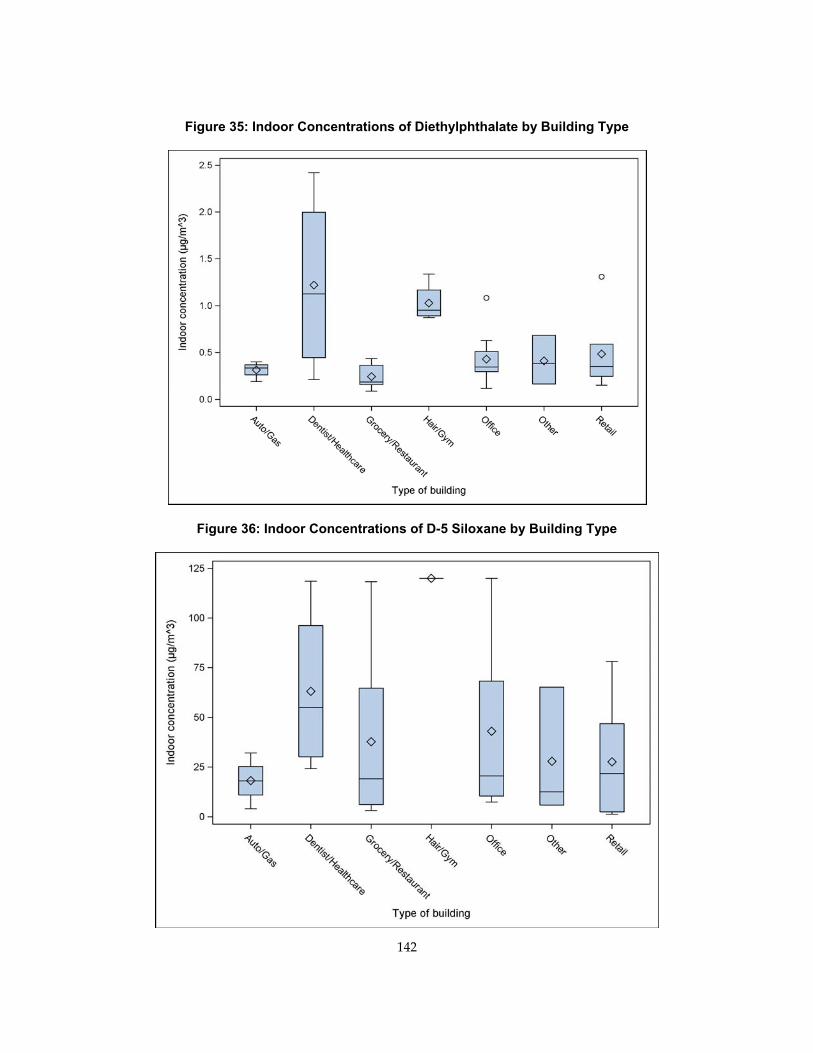
Figure 35: Indoor Concentrations of Diethylphthalate by Building Type

Figure 36: Indoor Concentrations of D-5 Siloxane by Building Type

 

142 

 

 

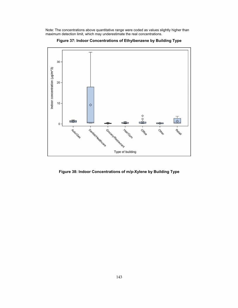
Note: The concentrations above quantitative range were coded as values slightly higher than maximum detection limit, which may underestimate the real concentrations.

Figure 37: Indoor Concentrations of Ethylbenzene by Building Type 

 

Figure 38: Indoor Concentrations of m/p-Xylene by Building Type

143 

 

 

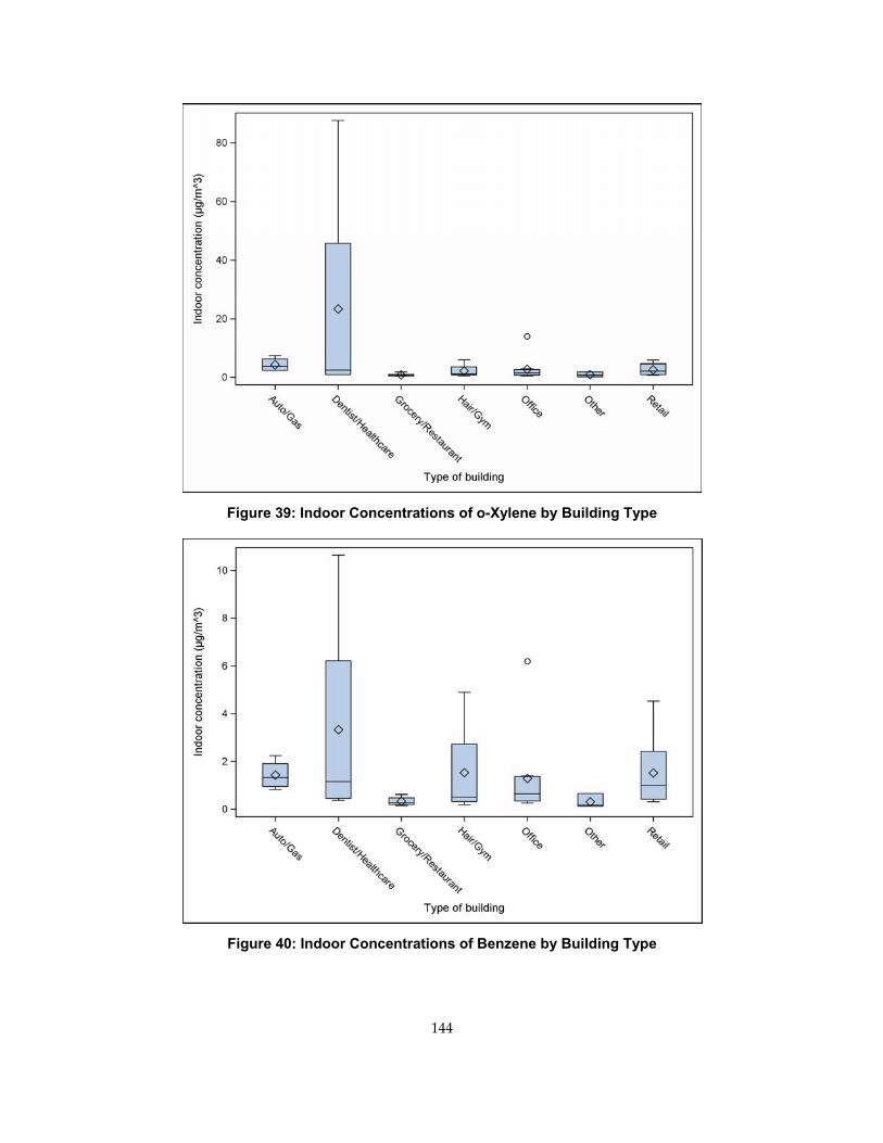
 Figure 39: Indoor Concentrations of o-Xylene by Building Type

 

Figure 40: Indoor Concentrations of Benzene by Building Type

144 

 

 

 

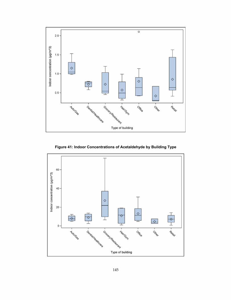
Figure 41: Indoor Concentrations of Acetaldehyde by Building Type

145 

 

 

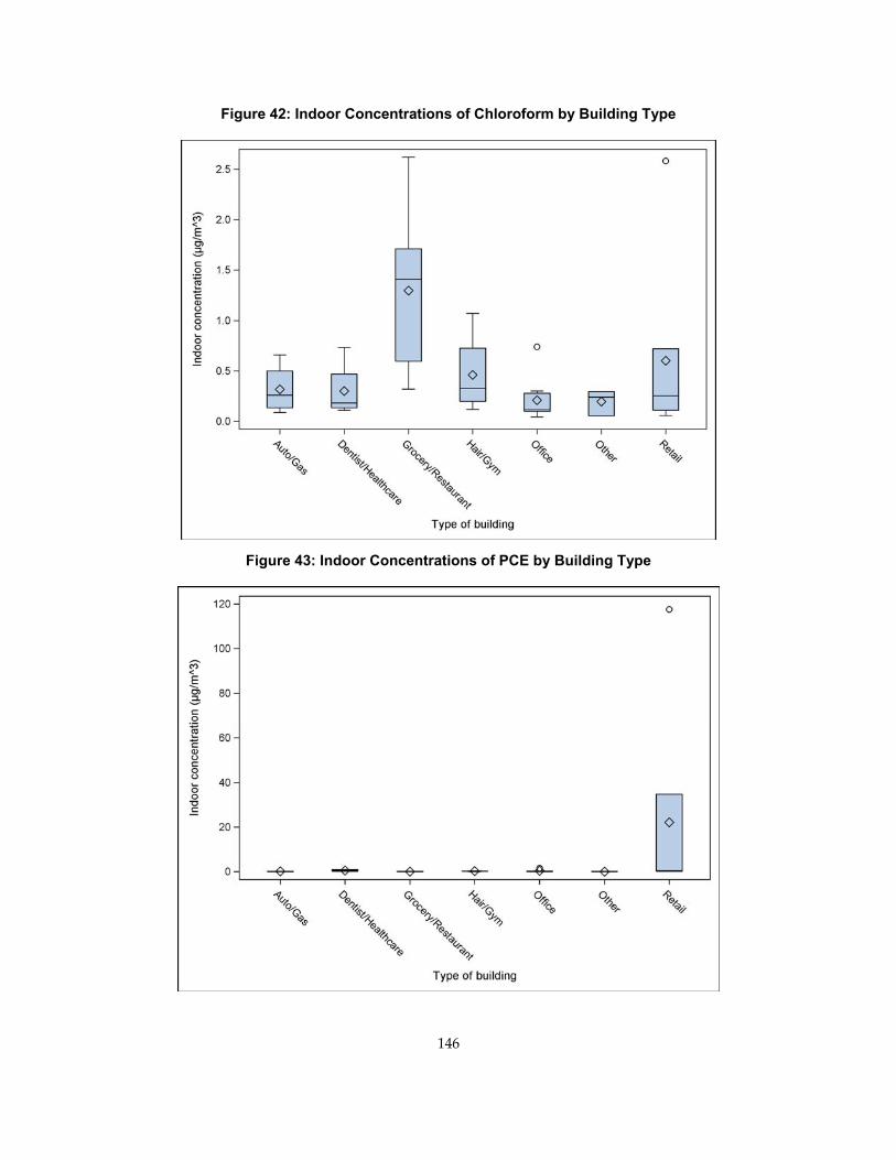
Figure 42: Indoor Concentrations of Chloroform by Building Type 

 Figure 43: Indoor Concentrations of PCE by Building Type 

 

 

146 

 

 

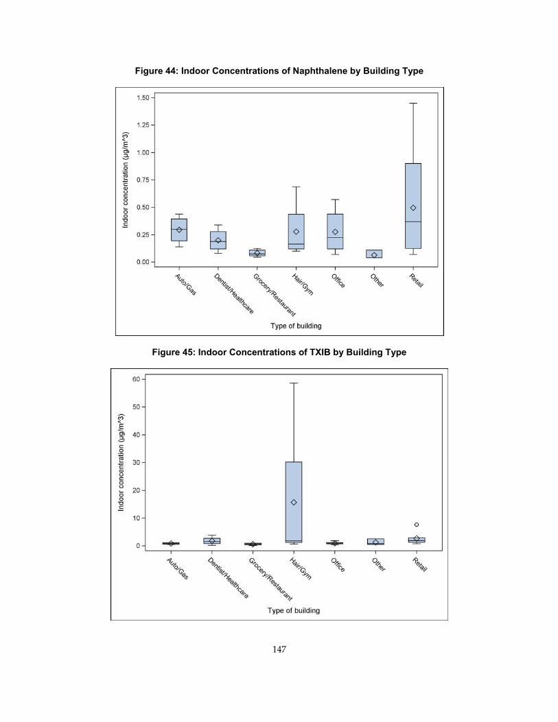
Figure 44: Indoor Concentrations of Naphthalene by Building Type 

Figure 45: Indoor Concentrations of TXIB by Building Type

147 

 

 

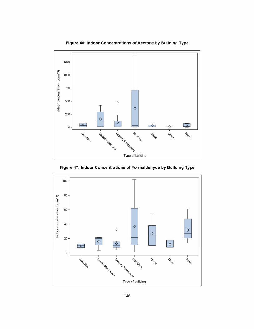
Figure 46: Indoor Concentrations of Acetone by Building Type

Figure 47: Indoor Concentrations of Formaldehyde by Building Type 

 

148 

 

 

 

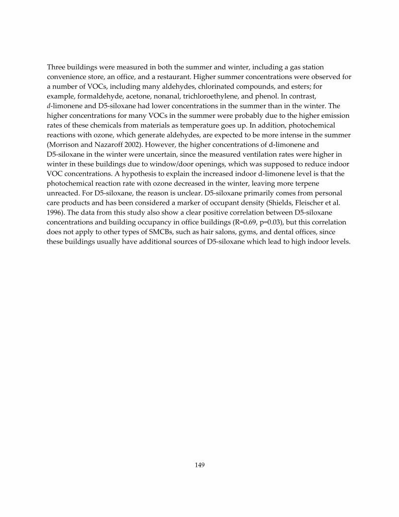
Three buildings were measured in both the summer and winter, including a gas station convenience store, an office, and a restaurant. Higher summer concentrations were observed for a number of VOCs, including many aldehydes, chlorinated compounds, and esters; for example, formaldehyde, acetone, nonanal, trichloroethylene, and phenol. In contrast, d‐limonene and D5‐siloxane had lower concentrations in the summer than in the winter. The higher concentrations for many VOCs in the summer were probably due to the higher emission rates of these chemicals from materials as temperature goes up. In addition, photochemical reactions with ozone, which generate aldehydes, are expected to be more intense in the summer (Morrison and Nazaroff 2002). However, the higher concentrations of d‐limonene and D5‐siloxane in the winter were uncertain, since the measured ventilation rates were higher in winter in these buildings due to window/door openings, which was supposed to reduce indoor VOC concentrations. A hypothesis to explain the increased indoor d‐limonene level is that the photochemical reaction rate with ozone decreased in the winter, leaving more terpene unreacted. For D5‐siloxane, the reason is unclear. D5‐siloxane primarily comes from personal care products and has been considered a marker of occupant density (Shields, Fleischer et al. 1996). The data from this study also show a clear positive correlation between D5‐siloxane concentrations and building occupancy in office buildings (R=0.69, p=0.03), but this correlation does not apply to other types of SMCBs, such as hair salons, gyms, and dental offices, since these buildings usually have additional sources of D5‐siloxane which lead to high indoor levels. 

149 

 

 

Building Source Strength The distributions of whole‐building source strength and whole‐building source strengths by area were calculated for the buildings with indoor/outdoor differences greater than zero; namely those having potential source(s), with results shown in Tables 49 and 50, respectively. All of the 30 VOCs had sources in more than 50 percent of the buildings, and 15 VOCs had potential sources in more than 90 percent of the buildings. The building source strengths by building type were calculated using the average indoor concentration of each building based on the method described in the Method section, and results are presented in Appendix G, Tables G.12–G.18.  

The compounds with the strongest source strength per area are acetone, D5‐siloxane, d‐limonene, 2‐butoxyethanol, and several aldehydes, basically consistent with the trend of indoor concentrations. D5‐siloxane building source strengths were generally high in all types of buildings, with the highest building source strengths, those exceeding 100 μg/m2h in grocery stores/restaurants, hair salons/gyms, and miscellaneous buildings, which might have high occupant density. The building source strengths of d‐limonene was particularly high in hair salons/gyms, while relatively low in gas station convenience store/fleet service buildings. Formaldehyde had high building source strengths in retail stores, and acetaldehyde had high building source strengths in grocery stores/restaurants. Nonanal presented higher building source strengths in grocery stores/restaurants and gas station convenience stores/ fleet service buildings, and hexanal and octanal appear to have similar emission profiles to nonanal. 

150 

 

 

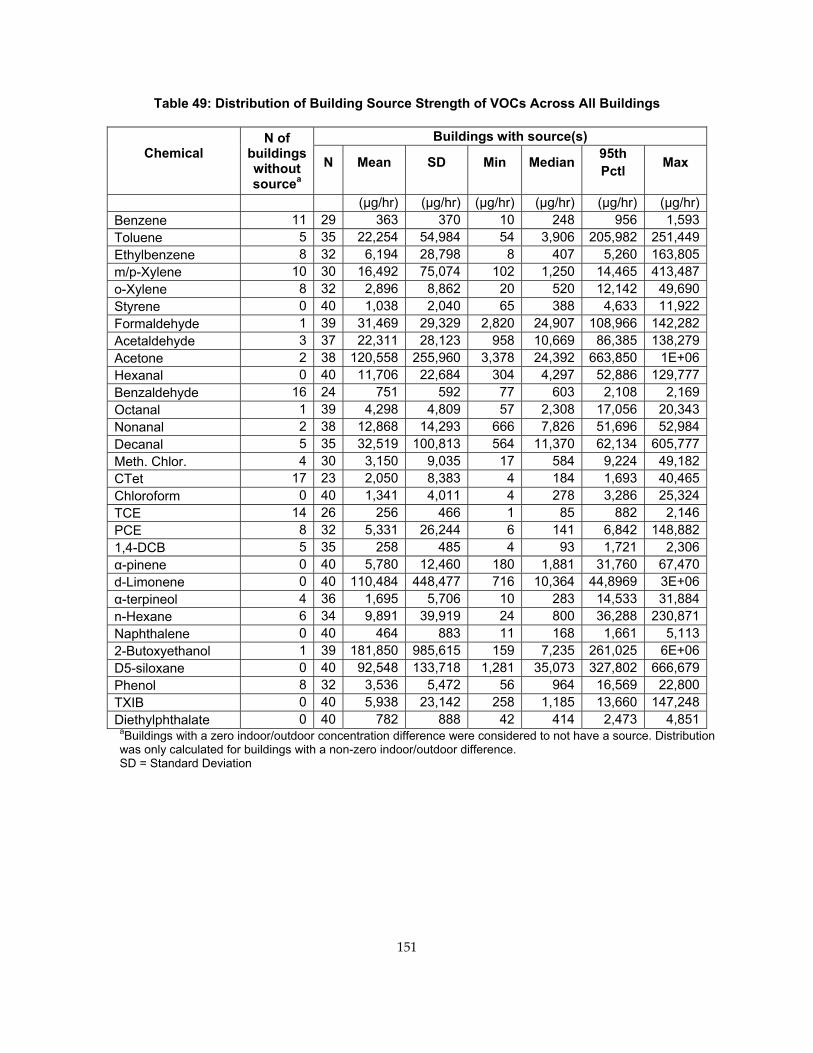
Table 49: Distribution of Building Source Strength of VOCs Across All Buildings  

Chemical N of

buildings without sourcea

Buildings with source(s)

N Mean SD Min Median 95th Pctl Max

(μg/hr) (μg/hr) (μg/hr) (μg/hr) (μg/hr) (μg/hr)Benzene 11 29 363 370 10 248 956 1,593Toluene 5 35 22,254 54,984 54 3,906 205,982 251,449Ethylbenzene 8 32 6,194 28,798 8 407 5,260 163,805m/p-Xylene 10 30 16,492 75,074 102 1,250 14,465 413,487o-Xylene 8 32 2,896 8,862 20 520 12,142 49,690Styrene 0 40 1,038 2,040 65 388 4,633 11,922Formaldehyde 1 39 31,469 29,329 2,820 24,907 108,966 142,282Acetaldehyde 3 37 22,311 28,123 958 10,669 86,385 138,279Acetone 2 38 120,558 255,960 3,378 24,392 663,850 1E+06Hexanal 0 40 11,706 22,684 304 4,297 52,886 129,777Benzaldehyde 16 24 751 592 77 603 2,108 2,169Octanal 1 39 4,298 4,809 57 2,308 17,056 20,343Nonanal 2 38 12,868 14,293 666 7,826 51,696 52,984Decanal 5 35 32,519 100,813 564 11,370 62,134 605,777Meth. Chlor. 4 30 3,150 9,035 17 584 9,224 49,182CTet 17 23 2,050 8,383 4 184 1,693 40,465Chloroform 0 40 1,341 4,011 4 278 3,286 25,324TCE 14 26 256 466 1 85 882 2,146PCE 8 32 5,331 26,244 6 141 6,842 148,8821,4-DCB 5 35 258 485 4 93 1,721 2,306α-pinene 0 40 5,780 12,460 180 1,881 31,760 67,470d-Limonene 0 40 110,484 448,477 716 10,364 44,8969 3E+06α-terpineol 4 36 1,695 5,706 10 283 14,533 31,884n-Hexane 6 34 9,891 39,919 24 800 36,288 230,871Naphthalene 0 40 464 883 11 168 1,661 5,1132-Butoxyethanol 1 39 181,850 985,615 159 7,235 261,025 6E+06D5-siloxane 0 40 92,548 133,718 1,281 35,073 327,802 666,679Phenol 8 32 3,536 5,472 56 964 16,569 22,800TXIB 0 40 5,938 23,142 258 1,185 13,660 147,248Diethylphthalate 0 40 782 888 42 414 2,473 4,851

aBuildings with a zero indoor/outdoor concentration difference were considered to not have a source. Distribution was only calculated for buildings with a non-zero indoor/outdoor difference. SD = Standard Deviation 

 

 

 

 

151 

 

 

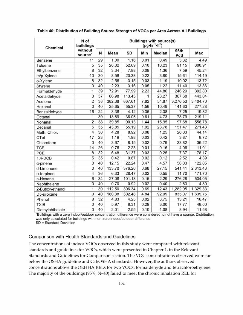
Table 40: Distribution of Building Source Strength of VOCs per Area Across All Buildings  

Chemical N of

buildings without sourcea

Buildings with source(s) (μg•hr-1•ft2)

N Mean SD Min Median 95th Pctl Max

Benzene 11 29 1.00 1.16 0.01 0.49 3.32 4.49Toluene 5 35 26.32 52.69 0.10 10.23 91.15 300.91Ethylbenzene 8 32 3.34 7.88 0.09 1.36 7.59 45.24m/p-Xylene 10 30 8.58 20.38 0.22 3.80 15.61 114.19o-Xylene 8 32 2.56 3.15 0.03 1.19 10.02 13.72Styrene 0 40 2.23 3.16 0.05 1.22 11.40 13.86Formaldehyde 1 39 72.91 77.99 2.23 44.86 246.29 392.80Acetaldehyde 3 37 66.98 113.45 1 23.27 367.68 443.04Acetone 2 38 382.38 867.61 7.82 54.87 3,276.53 3,404.70Hexanal 0 40 25.65 55.37 1.56 10.49 141.63 277.28Benzaldehyde 16 24 3.38 4.12 0.35 2.38 7.25 19.82Octanal 1 39 13.69 36.05 0.61 4.73 78.79 219.11Nonanal 2 38 39.85 90.13 1.44 15.95 97.68 556.78Decanal 5 35 43.85 55.19 1.92 23.78 151.47 271.43Meth. Chlor. 4 30 4.28 8.92 0.08 1.25 26.03 44.14CTet 17 23 1.19 1.98 0.03 0.42 3.87 8.72Chloroform 0 40 3.67 8.15 0.02 0.79 23.82 36.22TCE 14 26 0.76 2.23 0.01 0.16 4.06 11.01PCE 8 32 6.48 31.37 0.03 0.25 7.37 178.171,4-DCB 5 35 0.42 0.87 0.02 0.12 2.52 4.39α-pinene 0 40 12.15 22.24 0.47 4.57 56.03 122.05d-Limonene 0 40 133.70 376.20 0.68 27.15 541.41 2,313.43α-terpineol 4 36 6.33 28.47 0.02 0.55 11.70 171.70n-Hexane 6 34 27.08 101.13 0.15 2.29 276.28 534.05Naphthalene 0 40 0.70 0.92 0.02 0.40 2.63 4.802-Butoxyethanol 1 39 112.50 306.34 0.69 12.43 1,282.95 1,329.33D5-siloxane 0 40 180.38 302.48 4.84 92.99 835.07 1,635.75Phenol 8 32 4.83 4.25 0.02 3.75 13.21 16.47TXIB 0 40 5.97 8.31 0.29 3.00 17.77 48.00Diethylphthalate 0 40 2.01 2.55 0.10 1.08 8.94 11.58

aBuildings with a zero indoor/outdoor concentration difference were considered to not have a source. Distribution was only calculated for buildings with non-zero indoor/outdoor difference. SD = Standard Deviation 

 

Comparison with Health Standards and Guidelines The concentrations of indoor VOCs observed in this study were compared with relevant standards and guidelines for VOCs, which were presented in Chapter 1, in the Relevant Standards and Guidelines for Comparison section. The VOC concentrations observed were far below the OSHA guideline and Cal/OSHA standards. However, the authors observed concentrations above the OEHHA RELs for two VOCs: formaldehyde and tetrachloroethylene. The majority of the buildings (95%, N=40) failed to meet the chronic inhalation REL for 

152 

 

 

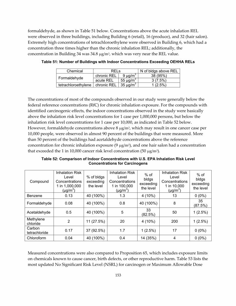
formaldehyde, as shown in Table 51 below. Concentrations above the acute inhalation REL were observed in three buildings, including Building 6 (retail), 16 (produce), and 32 (hair salon). Extremely high concentrations of tetrachloroethylene were observed in Building 6, which had a concentration three times higher than the chronic inhalation REL; additionally, the concentration in Building 34 was 34.8 μg/m3, which was very near the REL value.  

Table 51: Number of Buildings with Indoor Concentrations Exceeding OEHHA RELs

Chemical RELs N of bldgs above REL

Formaldehyde chronic REL 9 µg/m3 38 (95%) acute REL 55 µg/m3 3 (7.5%)

tetrachloroethylene chronic REL 35 µg/m3 1 (2.5%)  

The concentrations of most of the compounds observed in our study were generally below the federal reference concentrations (RfC) for chronic inhalation exposure. For the compounds with identified carcinogenic effects, the indoor concentrations observed in the study were basically above the inhalation risk level concentrations for 1 case per 1,000,000 persons, but below the inhalation risk level concentrations for 1 case per 10,000, as indicated in Table 52 below. However, formaldehyde concentrations above 8 μg/m3, which may result in one cancer case per 10,000 people, were observed in almost 90 percent of the buildings that were measured. More than 50 percent of the buildings had acetaldehyde concentrations above the reference concentration for chronic inhalation exposure (9 μg/m3), and one hair salon had a concentration that exceeded the 1 in 10,000 cancer risk level concentration (50 μg/m3).  

Table 52: Comparison of Indoor Concentrations with U.S. EPA Inhalation Risk Level Concentrations for Carcinogens

Compound

Inhalation Risk Level

Concentrations 1 in 1,000,000

(µg/m3)

% of bldgs exceeding the level

Inhalation Risk Level

Concentrations 1 in 100,000

(µg/m3)

% of bldgs

exceeding the level

Inhalation Risk Level

Concentrations 1 in 10,000

(µg/m3)

% of bldgs

exceeding the level

Benzene 0.13 40 (100%) 1.3 4 (10%) 13 0 (0%)

Formaldehyde 0.08 40 (100%) 0.8 40 (100%) 8 35 (87.5%)

Acetaldehyde 0.5 40 (100%) 5 33 (82.5%) 50 1 (2.5%)

Methylene chloride 2 11 (27.5%) 20 4 (10%) 200 1 (2.5%)

Carbon tetrachloride 0.17 37 (92.5%) 1.7 1 (2.5%) 17 0 (0%)

Chloroform 0.04 40 (100%) 0.4 14 (35%) 4 0 (0%)  

Measured concentrations were also compared to Proposition 65, which includes exposure limits on chemicals known to cause cancer, birth defects, or other reproductive harm. Table 53 lists the most updated No Significant Risk Level (NSRL) for carcinogen or Maximum Allowable Dose 

153 

 

 

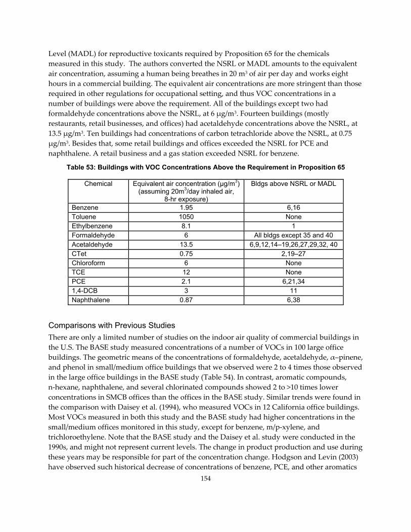
Level (MADL) for reproductive toxicants required by Proposition 65 for the chemicals measured in this study.  The authors converted the NSRL or MADL amounts to the equivalent air concentration, assuming a human being breathes in 20 m3 of air per day and works eight hours in a commercial building. The equivalent air concentrations are more stringent than those required in other regulations for occupational setting, and thus VOC concentrations in a number of buildings were above the requirement. All of the buildings except two had formaldehyde concentrations above the NSRL, at 6 μg/m3. Fourteen buildings (mostly restaurants, retail businesses, and offices) had acetaldehyde concentrations above the NSRL, at 13.5 μg/m3. Ten buildings had concentrations of carbon tetrachloride above the NSRL, at 0.75 μg/m3. Besides that, some retail buildings and offices exceeded the NSRL for PCE and naphthalene. A retail business and a gas station exceeded NSRL for benzene.   

Table 53: Buildings with VOC Concentrations Above the Requirement in Proposition 65

Chemical Equivalent air concentration (µg/m3) (assuming 20m3/day inhaled air,

8-hr exposure)

Bldgs above NSRL or MADL

Benzene 1.95 6,16 Toluene 1050 None Ethylbenzene 8.1 1 Formaldehyde 6 All bldgs except 35 and 40 Acetaldehyde 13.5 6,9,12,14–19,26,27,29,32, 40 CTet 0.75 2,19–27 Chloroform 6 None TCE 12 None PCE 2.1 6,21,34 1,4-DCB 3 11 Naphthalene 0.87 6,38

 

Comparisons with Previous Studies There are only a limited number of studies on the indoor air quality of commercial buildings in the U.S. The BASE study measured concentrations of a number of VOCs in 100 large office buildings. The geometric means of the concentrations of formaldehyde, acetaldehyde, α–pinene, and phenol in small/medium office buildings that we observed were 2 to 4 times those observed in the large office buildings in the BASE study (Table 54). In contrast, aromatic compounds, n‐hexane, naphthalene, and several chlorinated compounds showed 2 to >10 times lower concentrations in SMCB offices than the offices in the BASE study. Similar trends were found in the comparison with Daisey et al. (1994), who measured VOCs in 12 California office buildings. Most VOCs measured in both this study and the BASE study had higher concentrations in the small/medium offices monitored in this study, except for benzene, m/p‐xylene, and trichloroethylene. Note that the BASE study and the Daisey et al. study were conducted in the 1990s, and might not represent current levels. The change in product production and use during these years may be responsible for part of the concentration change. Hodgson and Levin (2003) have observed such historical decrease of concentrations of benzene, PCE, and other aromatics 

154 

 

 

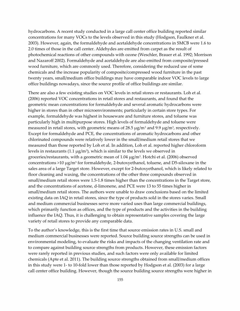
hydrocarbons. A recent study conducted in a large call center office building reported similar concentrations for many VOCs to the levels observed in this study (Hodgson, Faulkner et al. 2003). However, again, the formaldehyde and acetaldehyde concentrations in SMCB were 1.6 to 2.0 times of those in the call center. Aldehydes are emitted from carpet as the result of photochemical reactions of other compounds with ozone (Weschler, Brauer et al. 1992; Morrison and Nazaroff 2002). Formaldehyde and acetaldehyde are also emitted from composite/pressed wood furniture, which are commonly used. Therefore, considering the reduced use of some chemicals and the increase popularity of composite/compressed wood furniture in the past twenty years, small/medium office buildings may have comparable indoor VOC levels to large office buildings nowadays, since the source profile of office buildings are similar.  

There are also a few existing studies on VOC levels in retail stores or restaurants. Loh et al. (2006) reported VOC concentrations in retail stores and restaurants, and found that the geometric mean concentrations for formaldehyde and several aromatic hydrocarbons were higher in stores than in other microenvironments; particularly in certain store types. For example, formaldehyde was highest in houseware and furniture stores, and toluene was particularly high in multipurpose stores. High levels of formaldehyde and toluene were measured in retail stores, with geometric means of 28.5 μg/m3 and 9.9 μg/m3, respectively. Except for formaldehyde and PCE, the concentrations of aromatic hydrocarbons and other chlorinated compounds were relatively lower in the small/medium retail stores that we measured than those reported by Loh et al. In addition, Loh et al. reported higher chloroform levels in restaurants (1.1 μg/m3), which is similar to the levels we observed in groceries/restaurants, with a geometric mean of 1.04 μg/m3. Hotchi et al. (2006) observed concentrations >10 μg/m3 for formaldehyde, 2‐butoxyethanol, toluene, and D5‐siloxane in the sales area of a large Target store. However, except for 2‐butoxyethanol, which is likely related to floor cleaning and waxing, the concentrations of the other three compounds observed in small/medium retail stores were 1.5‐1.8 times higher than the concentrations in the Target store, and the concentrations of acetone, d‐limonene, and PCE were 13 to 55 times higher in small/medium retail stores. The authors were unable to draw conclusions based on the limited existing data on IAQ in retail stores, since the type of products sold in the stores varies. Small and medium commercial businesses serve more varied uses than large commercial buildings, which primarily function as offices, and the type of products and the activities in the building influence the IAQ. Thus, it is challenging to obtain representative samples covering the large variety of retail stores to provide any comparable data.  

To the author’s knowledge, this is the first time that source emission rates in U.S. small and medium commercial businesses were reported. Source building source strengths can be used in environmental modeling, to evaluate the risks and impacts of the changing ventilation rate and to compare against building source strengths from products. However, these emission factors were rarely reported in previous studies, and such factors were only available for limited chemicals (Apte et al. 2011). The building source strengths obtained from small/medium offices in this study were 1‐ to 10‐fold lower than those reported by Hodgson et al. (2003) for a large call center office building. However, though the source building source strengths were higher in 

155 

 

 

156 

 

the large call center office, the indoor VOC concentrations were similar, indicating a greater dilution rate from to the powerful ventilation systems of large buildings.  

Recently, Ongwandee et al. (2009) measured indoor and outdoor concentrations of formaldehyde and acetaldehyde in 12 office buildings in Thailand. They reported the building source strengths of 15.3 and 5.8 mg/h for formaldehyde and acetaldehyde, respectively, which were two to three times lower than the source strength obtained in this study (on average 31.2 mg/h for formaldehyde and 15.9 mg/h for acetaldehyde among 10 small/medium office buildings). However, due to the larger contribution from outdoor air, the indoor concentration of formaldehyde and acetaldehyde in their study were higher than what was observed in this study. 

 

 

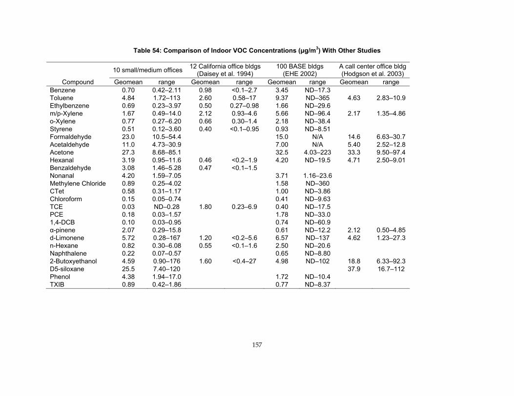
Table 54: Comparison of Indoor VOC Concentrations (μg/m3) With Other Studies

10 small/medium offices 12 California office bldgs (Daisey et al. 1994)

100 BASE bldgs (EHE 2002)

A call center office bldg (Hodgson et al. 2003)

Compound Geomean range Geomean range Geomean range Geomean range Benzene 0.70 0.42–2.11 0.98 <0.1–2.7 3.45 ND–17.3 Toluene 4.84 1.72–113 2.60 0.58–17 9.37 ND–365 4.63 2.83–10.9 Ethylbenzene 0.69 0.23–3.97 0.50 0.27–0.98 1.66 ND–29.6 m/p-Xylene 1.67 0.49–14.0 2.12 0.93–4.6 5.66 ND–96.4 2.17 1.35–4.86 o-Xylene 0.77 0.27–6.20 0.66 0.30–1.4 2.18 ND–38.4 Styrene 0.51 0.12–3.60 0.40 <0.1–0.95 0.93 ND–8.51 Formaldehyde 23.0 10.5–54.4 15.0 N/A 14.6 6.63–30.7 Acetaldehyde 11.0 4.73–30.9 7.00 N/A 5.40 2.52–12.8 Acetone 27.3 8.68–85.1 32.5 4.03–223 33.3 9.50–97.4 Hexanal 3.19 0.95–11.6 0.46 <0.2–1.9 4.20 ND–19.5 4.71 2.50–9.01 Benzaldehyde 3.08 1.46–5.28 0.47 <0.1–1.5 Nonanal 4.20 1.59–7.05 3.71 1.16–23.6 Methylene Chloride 0.89 0.25–4.02 1.58 ND–360 CTet 0.58 0.31–1.17 1.00 ND–3.86 Chloroform 0.15 0.05–0.74 0.41 ND–9.63 TCE 0.03 ND–0.28 1.80 0.23–6.9 0.40 ND–17.5 PCE 0.18 0.03–1.57 1.78 ND–33.0 1,4-DCB 0.10 0.03–0.95 0.74 ND–60.9 α-pinene 2.07 0.29–15.8 0.61 ND–12.2 2.12 0.50–4.85 d-Limonene 5.72 0.28–167 1.20 <0.2–5.6 6.57 ND–137 4.62 1.23–27.3 n-Hexane 0.82 0.30–6.08 0.55 <0.1–1.6 2.50 ND–20.6 Naphthalene 0.22 0.07–0.57 0.65 ND–8.80 2-Butoxyethanol 4.59 0.90–176 1.60 <0.4–27 4.98 ND–102 18.8 6.33–92.3 D5-siloxane 25.5 7.40–120 37.9 16.7–112 Phenol 4.38 1.94–17.0 1.72 ND–10.4 TXIB 0.89 0.42–1.86 0.77 ND–8.37

157 

 

 

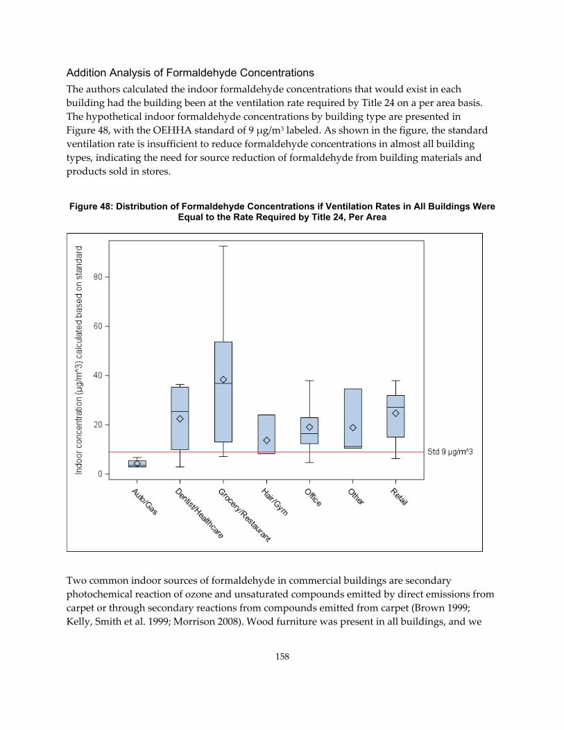
Addition Analysis of Formaldehyde Concentrations The authors calculated the indoor formaldehyde concentrations that would exist in each building had the building been at the ventilation rate required by Title 24 on a per area basis.  The hypothetical indoor formaldehyde concentrations by building type are presented in Figure 48, with the OEHHA standard of 9 μg/m3 labeled. As shown in the figure, the standard ventilation rate is insufficient to reduce formaldehyde concentrations in almost all building types, indicating the need for source reduction of formaldehyde from building materials and products sold in stores.  

Figure 48: Distribution of Formaldehyde Concentrations if Ventilation Rates in All Buildings Were Equal to the Rate Required by Title 24, Per Area

 

Two common indoor sources of formaldehyde in commercial buildings are secondary photochemical reaction of ozone and unsaturated compounds emitted by direct emissions from carpet or through secondary reactions from compounds emitted from carpet (Brown 1999; Kelly, Smith et al. 1999; Morrison 2008). Wood furniture was present in all buildings, and we 

158 

 

 

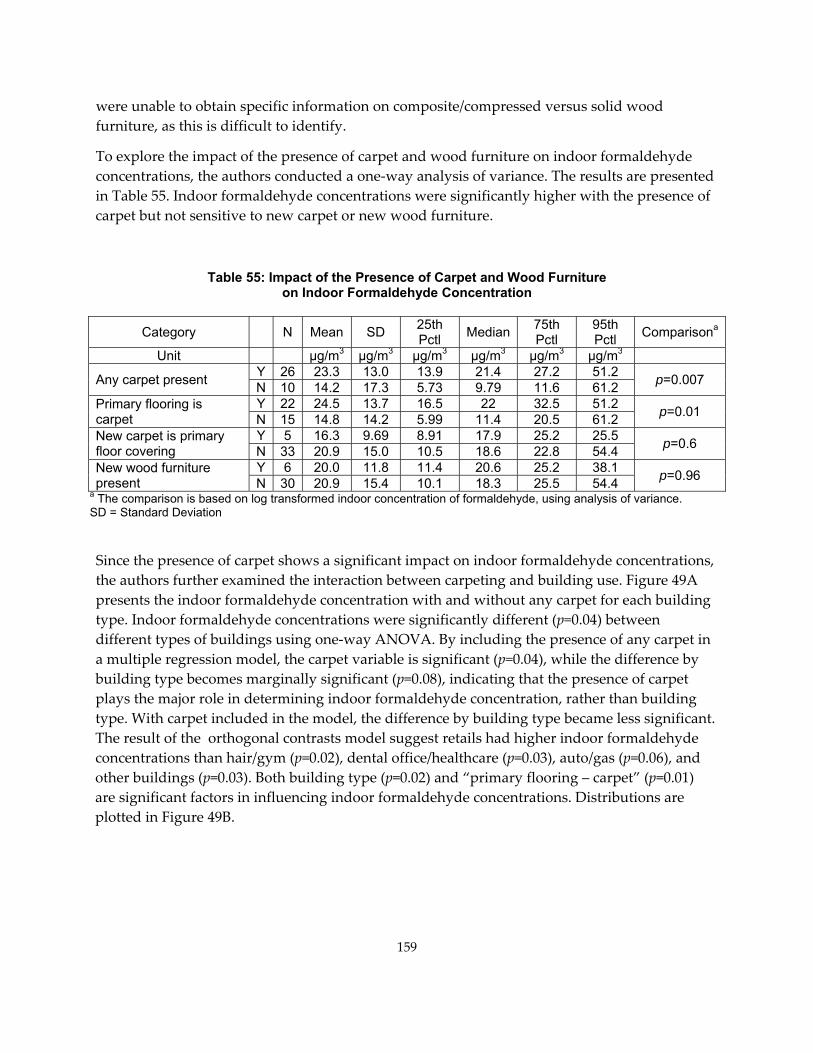
were unable to obtain specific information on composite/compressed versus solid wood furniture, as this is difficult to identify. 

To explore the impact of the presence of carpet and wood furniture on indoor formaldehyde concentrations, the authors conducted a one‐way analysis of variance. The results are presented in Table 55. Indoor formaldehyde concentrations were significantly higher with the presence of carpet but not sensitive to new carpet or new wood furniture. 

Table 55: Impact of the Presence of Carpet and Wood Furniture on Indoor Formaldehyde Concentration

Category N Mean SD 25th Pctl Median 75th

Pctl 95th

Pctl Comparisona

Unit μg/m3 μg/m3 μg/m3 μg/m3 μg/m3 μg/m3

Any carpet present Y 26 23.3 13.0 13.9 21.4 27.2 51.2 p=0.007 N 10 14.2 17.3 5.73 9.79 11.6 61.2 Primary flooring is carpet

Y 22 24.5 13.7 16.5 22 32.5 51.2 p=0.01 N 15 14.8 14.2 5.99 11.4 20.5 61.2 New carpet is primary floor covering

Y 5 16.3 9.69 8.91 17.9 25.2 25.5 p=0.6 N 33 20.9 15.0 10.5 18.6 22.8 54.4 New wood furniture present

Y 6 20.0 11.8 11.4 20.6 25.2 38.1 p=0.96 N 30 20.9 15.4 10.1 18.3 25.5 54.4 a The comparison is based on log transformed indoor concentration of formaldehyde, using analysis of variance. SD = Standard Deviation

Since the presence of carpet shows a significant impact on indoor formaldehyde concentrations, the authors further examined the interaction between carpeting and building use. Figure 49A presents the indoor formaldehyde concentration with and without any carpet for each building type. Indoor formaldehyde concentrations were significantly different (p=0.04) between different types of buildings using one‐way ANOVA. By including the presence of any carpet in a multiple regression model, the carpet variable is significant (p=0.04), while the difference by building type becomes marginally significant (p=0.08), indicating that the presence of carpet plays the major role in determining indoor formaldehyde concentration, rather than building type. With carpet included in the model, the difference by building type became less significant.  The result of the  orthogonal contrasts model suggest retails had higher indoor formaldehyde concentrations than hair/gym (p=0.02), dental office/healthcare (p=0.03), auto/gas (p=0.06), and other buildings (p=0.03). Both building type (p=0.02) and “primary flooring – carpet” (p=0.01) are significant factors in influencing indoor formaldehyde concentrations. Distributions are plotted in Figure 49B. 

159 

 

 

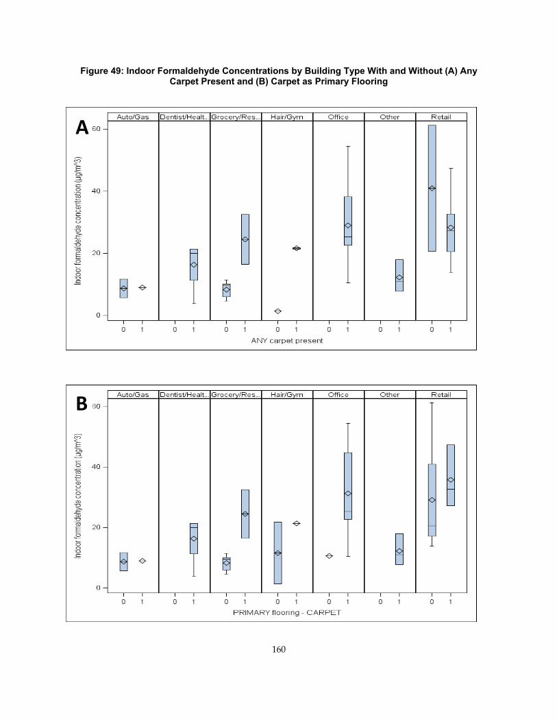
Figure 49: Indoor Formaldehyde Concentrations by Building Type With and Without (A) Any Carpet Present and (B) Carpet as Primary Flooring

 

 

A 

 

B 

160 

 

 

Factor Analysis for VOC Concentrations To identify indoor sources, the authors conducted a factor analysis on indoor VOC concentrations as defined in the statistical analysis plan. A total of 62 indoor observations are available to evaluate 30 compounds. The initial correlation analysis (Table 56) suggested that m/p‐xylene concentrations were highly correlated with ethylbenzene (R=0.97) and o‐xylene (R=0.96) concentrations, thus m/p‐xylene was excluded from the analysis. Methylene chloride was also excluded due to the potential solvent contamination for a number of samples mentioned previously.  

The first trial of factor analysis was conducted with 62 observations and 28 covariates. Though it was not statistically valid, it provided useful information to further refine the analysis and identify sources. Table 57 presents the results of the first trial after an oblique rotation and an orthogonal VARIMAX rotation. Seven factors with eigenvalue greater than 1 were extracted in this trial, which explains 64 percent of the variance in the indoor concentrations of the VOCs in the analysis.  

Factor 1 represents outdoor sources, with high loadings of benzene, toluene, ethylbenzene and xylenes (BTEX), and n‐hexane, primarily emitted from automatable sources. Factor 2 has high loadings of TXIB and diethylphthalate, which are plasticizers. Factor 3 represents low molecular weight aldehydes, and Factor 4 represents higher molecular weight aldehydes.  Factor 5 includes high loadings of d‐limonene, α‐terpineol, and D5‐siloxane, which are related to cleaning products. Factor 6 loads on chlorinated compounds, and Factor 7 may be related to restroom emissions (Weisel, Kim et al. 1999), but it is difficult to interpret the common origin of the compounds included in Factor 7. The residual analysis shows that the residual correlations are acceptable (0.048), but the partial correlations are relatively large (0.154), indicating that the factors may not fully explain the data, as the residual and partial correlations should be less than 0.1.  The high partial correlations are probably due to the large number of variables included in the analysis compared to relatively small number of observations. 

Based on the results of the first trial, the authors made a second attempt to confirm the findings in the first trial. To reduce the number of VOCs included in the analysis, only compounds with loadings > 0.5 on the first five factors extracted in the first trial were selected to be included, resulting in 14 compounds (as shown in Table 58). The second attempt obtained five factors, which explains 63 percent of the variance in the indoor concentrations of the VOCs in the analysis. Factor 1 is a simplified version of the Factor 1 in trial one, including benzene, toluene, ethylbenzene, and n‐hexane. Factor 2 confirms the pervious Factor 5, with high loadings of d‐limonene, α‐terpineol, and D5‐siloxane. Factor 3 represents high molecular weight aldehydes and Factor 5 represents low molecular weight aldehydes. Factor 4 represents the plasticizer sources. Since it was suspected that the plasticizer factor was driven by Building 18, a gym with recent floor renovation, we repeated the analysis without Building 18, and obtained basically the same factor pattern, with high loading of TXIB and diethylphthalate on Factor 4. The root mean squared off‐diagonal residual is 0.037 and the root mean squared partial correlation is 

161 

 

 

0.104, suggesting that the factors extracted can accurately account for the observed correlations among the 14 compounds.  

The sources highlighted in this analysis include automobile/traffic sources, cleaning products, occupant sources, wood products/coating, and plasticizers. Small‐ and medium‐sized commercial businesses are mostly located next to major roads and have parking lots close to the buildings; moreover, the building seal of SMCBs are usually not as tight as large commercial buildings. As a result, automobile sources appear to have larger impact on the IAQ in SMCBs. This factor related to automobiles was also observed in the analysis of the BASE study data (Apte and Erdmann 2002). Factor analysis also reveals air refreshers and cleaning sources that are represented by d‐limonene and α‐terpineol, and occupant sources, such as personal care products, presented by high loading of D5‐siloxane. Aldehydes usually appear into a single factor in previous studies (Apte and Erdmann 2002; Hodgson, Faulkner et al. 2003), which is associated with compressed wood products and furniture coating sources. However, in this analysis, the lower molecular weight and higher molecular weight aldehydes were extracted into two factors. TXIB and DEP appear in the same factor, indicating plasticized material sources. 

The authors briefly compared the factor analysis results to the factor analysis conducted based on data from the BASE study (Apte and Erdmann 2002), which focused on large office buildings. Since most of the compounds measured and the types of building included in these two studies were different, the factors obtained in these two analyses do not have much overlap. From the factor analysis of the BASE study VOC data, factors representing motor vehicles were obtained, including ethylbenzene, xylenes, and n‐hexane; however, different from our results, benzene and toluene were loaded on another factor representing “construction materials including ceiling panels and some insulation,” which was not observed in this study’s analysis. Another factor obtained from BASE data represents “Draperies fabric coverings and work station partitions,” including acetone and formaldehyde, while acetaldehyde was loaded on another factor about furniture coating and wood products. It was noted that both factor analyses were based on small samples; the results obtained may not be generalized.  

The investigators acknowledge that there are limitations in this analysis. There are only a small number of observations, and multiple observations were collected in the same building, which may not allow the construction of an unbiased correlation matrix. The analysis may not be statistically valid, though interpretable results were obtained. 

162 

 

 

  

Table 56: Pearson Correlation Coefficients Between Indoor VOC Concentrations

Pearson Correlation

Ben

zene

Tolu

ene

Eth

ylbe

nzen

e

m/p

-Xyl

ene

o-Xy

lene

Sty

rene

Form

alde

hyde

Acet

alde

hyde

Ace

tone

Hex

anal

Benz

alde

hyde

Oct

anal

Non

anal

Dec

anal

Benzene Toluene .48

Ethylbenzene .59 .53 m/p-Xylene .61 .58 .97

o-Xylene .60 .55 .94 .96 Styrene .62 .54 .54 .54 .55

Formaldehyde .12 .34 -.10 -.12 .04 .39 Acetaldehyde .06 .26 -.18 -.13 -.04 .30 .60

Acetone -.01 .41 -.04 -.01 .04 .21 .49 .64 Hexanal .34 .30 .60 .55 .54 .46 -.01 .14 .15

Benzaldehyde .74 .16 .30 .35 .35 .46 .52 .31 .34 .39 Octanal .41 -.04 .26 .27 .28 .29 -.01 .05 -.11 .42 .50 Nonanal .47 -.16 .13 .14 .14 .27 -.06 .01 -.27 .34 .62 .78 Decanal .39 .07 .22 .23 .25 .27 .12 .11 .02 .14 .39 .54 .60

Meth. Chlor. .33 .07 .22 .31 .30 .32 .04 .01 -.02 -.01 .38 .14 .19 .25 CTet .59 -.08 .14 .16 .16 .28 -.03 -.04 -.29 .20 .80 .48 .66 .47

Chloroform .15 .15 -.10 -.08 -.10 .21 .16 .32 .28 .27 .19 .10 .06 .08 TCE .13 .48 .24 .20 .18 .22 .10 .00 .22 .06 -.04 -.23 -.21 -.03 PCE .28 .25 .28 .27 .35 .22 .16 -.06 -.04 -.04 .15 .01 .01 -.10

1,4-DCB .21 .02 .14 .13 .20 .15 .08 -.08 -.09 -.05 .33 .08 .08 .10 α-pinene .39 .49 .33 .39 .38 .64 .48 .25 .23 .39 .32 .20 .14 .12

d-Limonene .36 .46 .34 .39 .37 .46 .03 .00 .08 .30 .14 .18 .14 .02 α-terpineol .33 .51 .35 .41 .38 .54 .17 .16 .28 .27 .12 .03 -.02 .09 n-Hexane .50 .54 .43 .48 .49 .40 .28 -.03 .00 .21 .22 .02 -.07 -.13

Naphthalene .46 .59 .55 .64 .67 .54 .37 .10 .13 .38 .37 .19 .16 .19 2-Butoxyethanol .37 .31 .34 .29 .34 .27 .01 .07 -.03 .21 .21 .16 .09 .23

D5-siloxane -.04 .24 .11 .17 .19 .20 .08 .20 .33 .13 -.09 -.15 -.20 -.18 Phenol .51 .32 .31 .35 .37 .55 .49 .29 .24 .26 .58 .35 .35 .36 TXIB .24 .31 .28 .45 .48 .39 .40 .11 .17 .31 .39 .27 .27 .12

Diethylphthalate .24 .28 .23 .35 .34 .38 .30 .06 .32 .25 .37 .14 .09 -.06 Note: Correlation coefficients were calculated based on log-transformed indoor VOC concentrations. 

163 

 

 

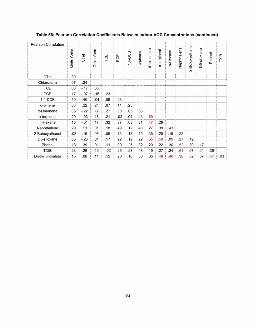
Table 56: Pearson Correlation Coefficients Between Indoor VOC Concentrations (continued)

Pearson Correlation

Met

h. C

hlor

.

CTe

t

Chl

orof

orm

TCE

PC

E

1,4-

DC

B

α-pi

nene

d-Li

mon

ene

α-te

rpin

eol

n-H

exan

e

Nap

htha

lene

2-B

utox

yeth

anol

D5-

silo

xane

Phen

ol

TXIB

CTet .39 Chloroform .07 .24

TCE .08 -.17 .06 PCE .17 -.07 -.15 .23

1,4-DCB .19 .40 -.04 .09 .23 α-pinene .08 .22 .24 .07 .14 .23

d-Limonene .05 -.22 .12 .27 .30 .03 .33 α-terpineol .20 -.03 .18 .21 -.02 .04 .43 .59 n-Hexane .15 -.01 .17 .32 .37 .03 .31 .47 .29

Naphthalene .29 .11 .01 .18 .49 .12 .46 .27 .39 .43 2-Butoxyethanol -.03 .19 .06 .05 .16 .18 .15 .35 .20 .19 .22

D5-siloxane .03 -.26 .01 .17 .22 .12 .22 .55 .59 .09 .27 .19 Phenol .18 .39 .01 .11 .30 .25 .32 .20 .22 .30 .52 .30 .17 TXIB .23 .26 .10 -.02 .25 .23 .48 .19 .27 .24 .61 .07 .21 .36

Diethylphthalate .15 .08 .11 .12 .20 .16 .30 .35 .48 .40 .38 .02 .37 .47 .63

 

164 

 

 

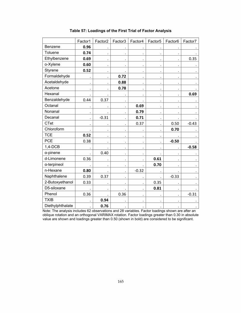
Table 57: Loadings of the First Trial of Factor Analysis

Factor1 Factor2 Factor3 Factor4 Factor5 Factor6 Factor7Benzene 0.96  . . . . .  .Toluene 0.74  . . . . .  .Ethylbenzene 0.69  . . . . .  0.35o-Xylene 0.60  . . . . .  .Styrene 0.52  . . . . .  .Formaldehyde .  . 0.72 . . .  .Acetaldehyde .  . 0.88 . . .  .Acetone .  . 0.78 . . .  .Hexanal .  . . . . .  0.69Benzaldehyde 0.44  0.37 . . . .  .Octanal .  . . 0.69 . .  .Nonanal .  . . 0.79 . .  .Decanal .  ‐0.31 . 0.71 . .  .CTet .  . . 0.37 . 0.50  ‐0.43Chloroform .  . . . . 0.70  .TCE 0.52  . . . . .  .PCE 0.38  . . . . ‐0.50  .1,4-DCB .  . . . . .  ‐0.58α-pinene .  0.40 . . . .  .d-Limonene 0.36  . . . 0.61 .  .α-terpineol .  . . . 0.70 .  .n-Hexane 0.80  . . ‐0.32 . .  .Naphthalene 0.39  0.37 . . . ‐0.33  .2-Butoxyethanol 0.33  . . . 0.35 .  .D5-siloxane .  . . . 0.81 .  .Phenol 0.36  . 0.36 . . .  ‐0.31TXIB .  0.94 . . . .  .Diethylphthalate .  0.76 . . . .  .

Note: The analysis includes 62 observations and 28 variables. Factor loadings shown are after an oblique rotation and an orthogonal VARIMAX rotation. Factor loadings greater than 0.30 in absolute value are shown and loadings greater than 0.50 (shown in bold) are considered to be significant.

165 

 

 

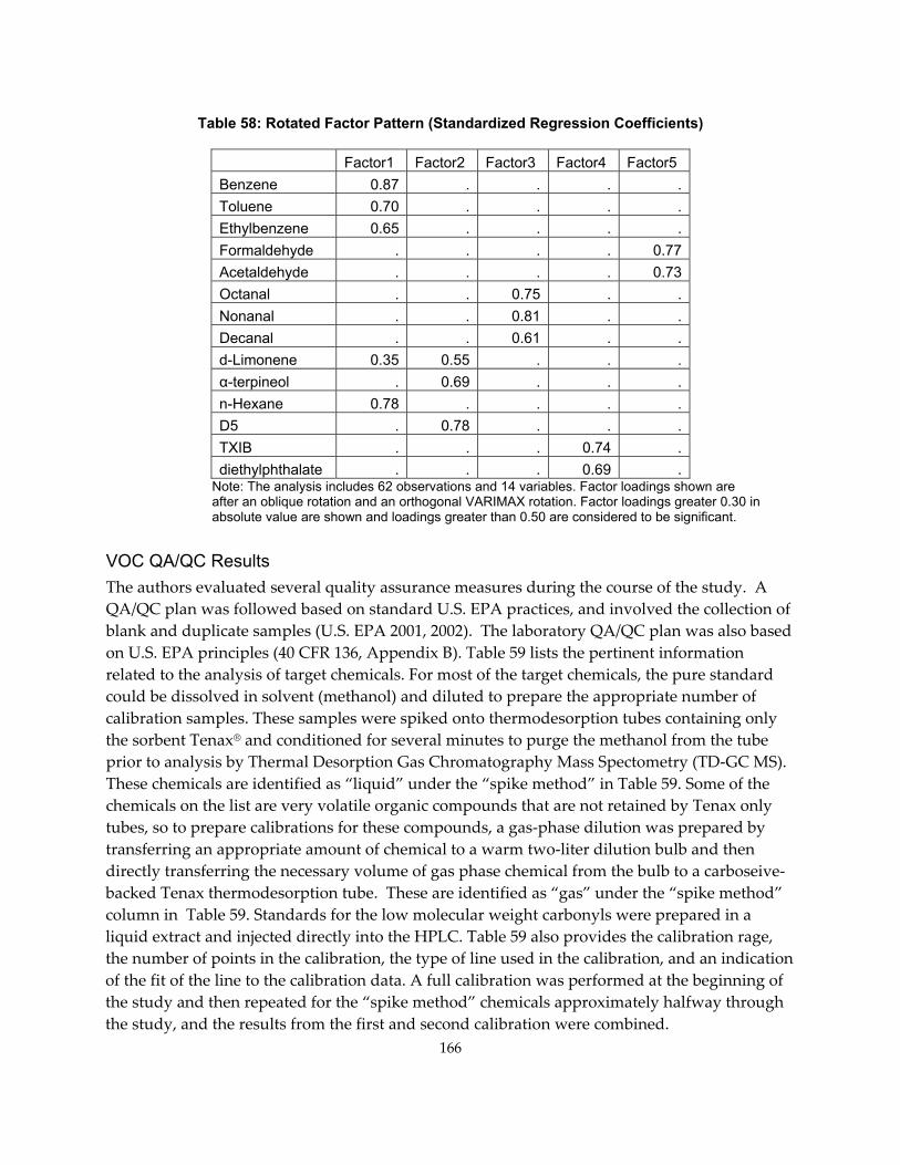
Table 58: Rotated Factor Pattern (Standardized Regression Coefficients)

Factor1 Factor2 Factor3 Factor4 Factor5 Benzene 0.87 . . . . Toluene 0.70 . . . . Ethylbenzene 0.65 . . . . Formaldehyde . . . . 0.77 Acetaldehyde . . . . 0.73 Octanal . . 0.75 . . Nonanal . . 0.81 . . Decanal . . 0.61 . . d-Limonene 0.35 0.55 . . . α-terpineol . 0.69 . . . n-Hexane 0.78 . . . . D5 . 0.78 . . . TXIB . . . 0.74 . diethylphthalate . . . 0.69 .

Note: The analysis includes 62 observations and 14 variables. Factor loadings shown are after an oblique rotation and an orthogonal VARIMAX rotation. Factor loadings greater 0.30 in absolute value are shown and loadings greater than 0.50 are considered to be significant.

 VOC QA/QC Results The authors evaluated several quality assurance measures during the course of the study.  A QA/QC plan was followed based on standard U.S. EPA practices, and involved the collection of blank and duplicate samples (U.S. EPA 2001, 2002).  The laboratory QA/QC plan was also based on U.S. EPA principles (40 CFR 136, Appendix B). Table 59 lists the pertinent information related to the analysis of target chemicals. For most of the target chemicals, the pure standard could be dissolved in solvent (methanol) and diluted to prepare the appropriate number of calibration samples. These samples were spiked onto thermodesorption tubes containing only the sorbent Tenax® and conditioned for several minutes to purge the methanol from the tube prior to analysis by Thermal Desorption Gas Chromatography Mass Spectometry (TD‐GC MS). These chemicals are identified as “liquid” under the “spike method” in Table 59. Some of the chemicals on the list are very volatile organic compounds that are not retained by Tenax only tubes, so to prepare calibrations for these compounds, a gas‐phase dilution was prepared by transferring an appropriate amount of chemical to a warm two‐liter dilution bulb and then directly transferring the necessary volume of gas phase chemical from the bulb to a carboseive‐backed Tenax thermodesorption tube.  These are identified as “gas” under the “spike method” column in  Table 59. Standards for the low molecular weight carbonyls were prepared in a liquid extract and injected directly into the HPLC. Table 59 also provides the calibration rage, the number of points in the calibration, the type of line used in the calibration, and an indication of the fit of the line to the calibration data. A full calibration was performed at the beginning of the study and then repeated for the “spike method” chemicals approximately halfway through the study, and the results from the first and second calibration were combined. 

166 

 

 

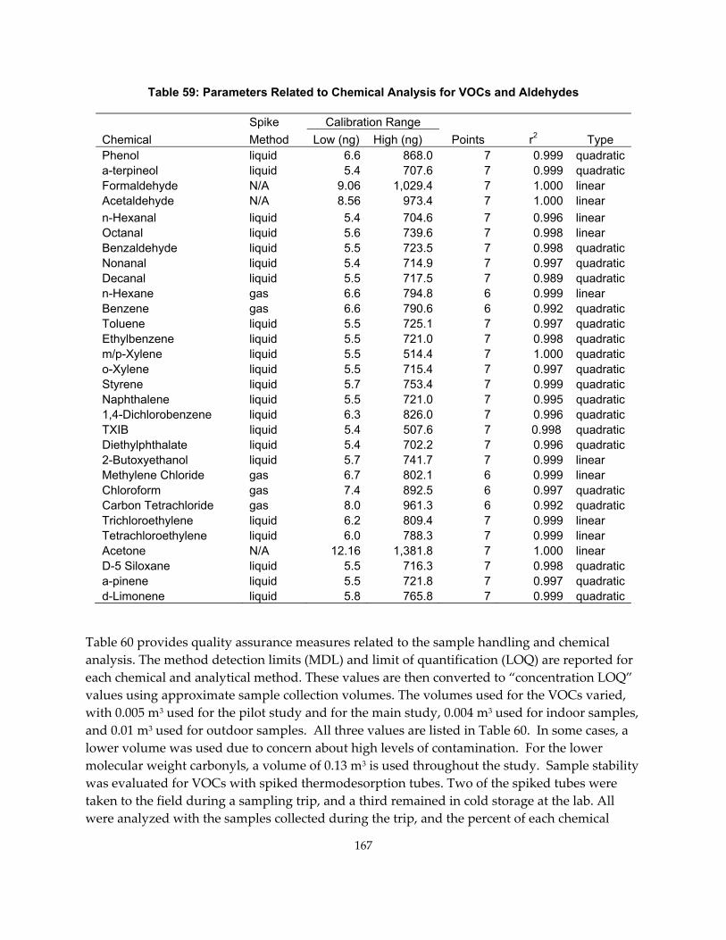
Table 59: Parameters Related to Chemical Analysis for VOCs and Aldehydes

Spike Calibration Range Chemical Method Low (ng) High (ng) Points r2 Type Phenol liquid 6.6 868.0 7 0.999 quadratica-terpineol liquid 5.4 707.6 7 0.999 quadraticFormaldehyde N/A 9.06 1,029.4 7 1.000 linear Acetaldehyde N/A 8.56 973.4 7 1.000 linear n-Hexanal liquid 5.4 704.6 7 0.996 linear Octanal liquid 5.6 739.6 7 0.998 linear Benzaldehyde liquid 5.5 723.5 7 0.998 quadraticNonanal liquid 5.4 714.9 7 0.997 quadraticDecanal liquid 5.5 717.5 7 0.989 quadraticn-Hexane gas 6.6 794.8 6 0.999 linear Benzene gas 6.6 790.6 6 0.992 quadraticToluene liquid 5.5 725.1 7 0.997 quadraticEthylbenzene liquid 5.5 721.0 7 0.998 quadraticm/p-Xylene liquid 5.5 514.4 7 1.000 quadratico-Xylene liquid 5.5 715.4 7 0.997 quadraticStyrene liquid 5.7 753.4 7 0.999 quadraticNaphthalene liquid 5.5 721.0 7 0.995 quadratic1,4-Dichlorobenzene liquid 6.3 826.0 7 0.996 quadraticTXIB liquid 5.4 507.6 7 0.998 quadraticDiethylphthalate liquid 5.4 702.2 7 0.996 quadratic2-Butoxyethanol liquid 5.7 741.7 7 0.999 linear Methylene Chloride gas 6.7 802.1 6 0.999 linear Chloroform gas 7.4 892.5 6 0.997 quadraticCarbon Tetrachloride gas 8.0 961.3 6 0.992 quadraticTrichloroethylene liquid 6.2 809.4 7 0.999 linear Tetrachloroethylene liquid 6.0 788.3 7 0.999 linear Acetone N/A 12.16 1,381.8 7 1.000 linear D-5 Siloxane liquid 5.5 716.3 7 0.998 quadratica-pinene liquid 5.5 721.8 7 0.997 quadraticd-Limonene liquid 5.8 765.8 7 0.999 quadratic

Table 60 provides quality assurance measures related to the sample handling and chemical analysis. The method detection limits (MDL) and limit of quantification (LOQ) are reported for each chemical and analytical method. These values are then converted to “concentration LOQ” values using approximate sample collection volumes. The volumes used for the VOCs varied, with 0.005 m3 used for the pilot study and for the main study, 0.004 m3 used for indoor samples, and 0.01 m3 used for outdoor samples.  All three values are listed in Table 60.  In some cases, a lower volume was used due to concern about high levels of contamination.  For the lower molecular weight carbonyls, a volume of 0.13 m3 is used throughout the study.  Sample stability was evaluated for VOCs with spiked thermodesorption tubes. Two of the spiked tubes were taken to the field during a sampling trip, and a third remained in cold storage at the lab. All were analyzed with the samples collected during the trip, and the percent of each chemical 

167 

 

 

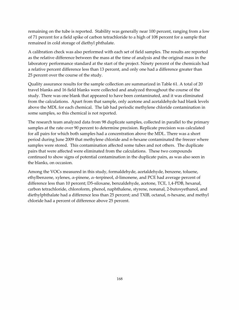
remaining on the tube is reported.  Stability was generally near 100 percent, ranging from a low of 71 percent for a field spike of carbon tetrachloride to a high of 108 percent for a sample that remained in cold storage of diethyl phthalate.  

A calibration check was also performed with each set of field samples. The results are reported as the relative difference between the mass at the time of analysis and the original mass in the laboratory performance standard at the start of the project. Ninety percent of the chemicals had a relative percent difference less than 13 percent, and only one had a difference greater than 25 percent over the course of the study. 

Quality assurance results for the sample collection are summarized in Table 61. A total of 20 travel blanks and 16 field blanks were collected and analyzed throughout the course of the study. There was one blank that appeared to have been contaminated, and it was eliminated from the calculations.  Apart from that sample, only acetone and acetaldehyde had blank levels above the MDL for each chemical.  The lab had periodic methylene chloride contamination in some samples, so this chemical is not reported. 

The research team analyzed data from 98 duplicate samples, collected in parallel to the primary samples at the rate over 90 percent to determine precision. Replicate precision was calculated for all pairs for which both samples had a concentration above the MDL. There was a short period during June 2009 that methylene chloride and n‐hexane contaminated the freezer where samples were stored.  This contamination affected some tubes and not others.  The duplicate pairs that were affected were eliminated from the calculations.  These two compounds continued to show signs of potential contamination in the duplicate pairs, as was also seen in the blanks, on occasion.   

Among the VOCs measured in this study, formaldehyde, acetaldehyde, benzene, toluene, ethylbenzene, xylenes, α‐pinene, α–terpineol, d‐limonene, and PCE had average percent of difference less than 10 percent; D5‐siloxane, benzaldehyde, acetone, TCE, 1,4‐PDB, hexanal, carbon tetrachloride, chloroform, phenol, naphthalene, styrene, nonanal, 2‐butoxyethanol, and diethylphthalate had a difference less than 25 percent; and TXIB, octanal, n‐hexane, and methyl chloride had a percent of difference above 25 percent. 

 

 

 

 

 

 

168 

 

 

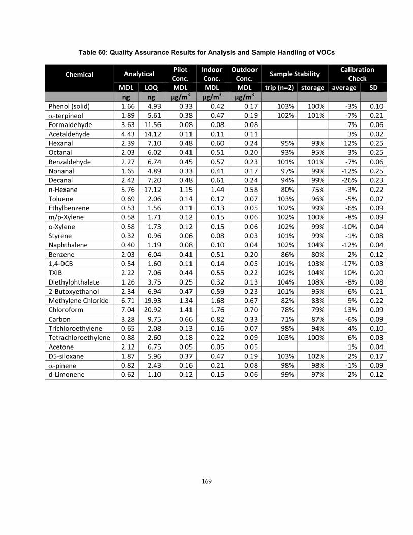
Table 60: Quality Assurance Results for Analysis and Sample Handling of VOCs

Chemical  Analytical Pilot Conc.

Indoor Conc.

Outdoor Conc.

Sample Stability Calibration 

CheckMDL  LOQ  MDL MDL MDL trip (n=2)  storage  average SD

  ng  ng  μg/m3 μg/m3 μg/m3  Phenol (solid)  1.66  4.93  0.33 0.42 0.17 103%  100%  ‐3% 0.10α‐terpineol  1.89  5.61  0.38 0.47 0.19 102%  101%  ‐7% 0.21Formaldehyde  3.63  11.56  0.08 0.08 0.08     7% 0.06Acetaldehyde  4.43  14.12  0.11 0.11 0.11     3% 0.02Hexanal  2.39  7.10  0.48 0.60 0.24 95%  93%  12% 0.25Octanal  2.03  6.02  0.41 0.51 0.20 93%  95%  3% 0.25Benzaldehyde  2.27  6.74  0.45 0.57 0.23 101%  101%  ‐7% 0.06Nonanal  1.65  4.89  0.33 0.41 0.17 97%  99%  ‐12% 0.25Decanal  2.42  7.20  0.48 0.61 0.24 94%  99%  ‐26% 0.23n‐Hexane  5.76  17.12  1.15 1.44 0.58 80%  75%  ‐3% 0.22Toluene  0.69  2.06  0.14 0.17 0.07 103%  96%  ‐5% 0.07Ethylbenzene  0.53  1.56  0.11 0.13 0.05 102%  99%  ‐6% 0.09m/p‐Xylene  0.58  1.71  0.12 0.15 0.06 102%  100%  ‐8% 0.09o‐Xylene  0.58  1.73  0.12 0.15 0.06 102%  99%  ‐10% 0.04Styrene  0.32  0.96  0.06 0.08 0.03 101%  99%  ‐1% 0.08Naphthalene  0.40  1.19  0.08 0.10 0.04 102%  104%  ‐12% 0.04Benzene  2.03  6.04  0.41 0.51 0.20 86%  80%  ‐2% 0.121,4‐DCB  0.54  1.60  0.11 0.14 0.05 101%  103%  ‐17% 0.03TXIB  2.22  7.06  0.44 0.55 0.22 102%  104%  10% 0.20Diethylphthalate  1.26  3.75  0.25 0.32 0.13 104%  108%  ‐8% 0.082‐Butoxyethanol  2.34  6.94  0.47 0.59 0.23 101%  95%  ‐6% 0.21Methylene Chloride  6.71  19.93  1.34 1.68 0.67 82%  83%  ‐9% 0.22Chloroform  7.04  20.92  1.41 1.76 0.70 78%  79%  13% 0.09Carbon  3.28  9.75  0.66 0.82 0.33 71%  87%  ‐6% 0.09Trichloroethylene  0.65  2.08  0.13 0.16 0.07 98%  94%  4% 0.10Tetrachloroethylene  0.88  2.60  0.18 0.22 0.09 103%  100%  ‐6% 0.03Acetone  2.12  6.75  0.05 0.05 0.05     1% 0.04D5‐siloxane  1.87  5.96  0.37 0.47 0.19 103%  102%  2% 0.17α‐pinene  0.82  2.43  0.16 0.21 0.08 98%  98%  ‐1% 0.09d‐Limonene  0.62  1.10  0.12 0.15 0.06 99%  97%  ‐2% 0.12 

169 

 

 

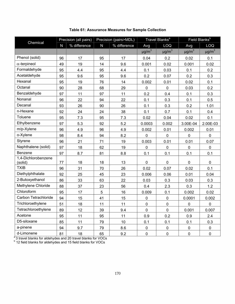
Table 61: Assurance Measures for Sample Collection

Chemical Precision (all pairs) Precision (pairs>MDL) Travel Blanksa Field Blanksb N % difference N % difference Avg LOQ Avg LOQ

µg/m3 µg/m3 µg/m3 µg/m3 Phenol (solid) 96 17 95 17 0.04 0.2 0.02 0.1 α-terpineol 49 19 14 9.6 0.001 0.02 0.001 0.02 Formaldehyde 95 4.4 95 4.4 0.1 0.03 0.1 0.2 Acetaldehyde 95 9.6 95 9.6 0.2 0.07 0.2 0.3 Hexanal 95 19 76 14 0.002 0.01 0.02 0.1 Octanal 90 28 68 29 0 0 0.03 0.2 Benzaldehyde 97 11 97 11 0.2 0.4 0.1 0.3 Nonanal 96 22 94 22 0.1 0.3 0.1 0.5 Decanal 93 26 90 26 0.1 0.3 0.2 1.01 n-Hexane 92 24 24 38 0.1 0.7 0.1 0.4 Toluene 95 7.3 95 7.3 0.02 0.04 0.02 0.1 Ethylbenzene 97 5.3 92 5.2 0.0003 0.002 3.00E-04 2.00E-03 m/p-Xylene 96 4.9 96 4.9 0.002 0.01 0.002 0.01 o-Xylene 98 8.4 94 8.2 0 0 0 0 Styrene 96 21 71 19 0.003 0.01 0.01 0.07 Naphthalene (solid) 97 18 62 19 0 0 0 0 Benzene 97 8.7 81 8.8 0.1 0.1 0.1 0.1 1,4-Dichlorobenzene (solid) 77 18 18 13 0 0 0 0 TXIB 96 31 70 26 0.02 0.07 0.02 0.1 Diethylphthalate 92 25 45 23 0.006 0.06 0.01 0.04 2-Butoxyethanol 86 33 63 22 0.03 0.3 0.03 0.3 Methylene Chloride 88 37 23 56 0.4 2.3 0.3 1.2 Chloroform 95 17 5 16 0.009 0.1 0.002 0.02 Carbon Tetrachloride 94 15 41 15 0 0 0.0001 0.002 Trichloroethylene 51 18 11 11 0 0 0 0 Tetrachloroethylene 89 12 39 9.4 0 0 0.001 0.007 Acetone 95 11 95 11 0.9 0.2 0.9 2.4 D5-siloxane 85 11 79 10 0.1 0.1 0.1 0.3 a-pinene 94 9.7 79 8.6 0 0 0 0 d-Limonene 81 18 65 9.2 0 0 0 0

a 3 travel blanks for aldehydes and 20 travel blanks for VOCs b 12 field blanks for aldehydes and 15 field blanks for VOCs

 

170 

 

 

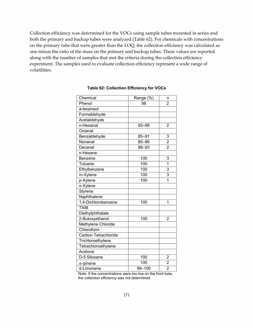
Collection efficiency was determined for the VOCs using sample tubes mounted in series and both the primary and backup tubes were analyzed (Table 62). For chemicals with concentrations on the primary tube that were greater than the LOQ, the collection efficiency was calculated as one minus the ratio of the mass on the primary and backup tubes. These values are reported along with the number of samples that met the criteria during the collection efficiency experiment. The samples used to evaluate collection efficiency represent a wide range of volatilities.   

 

Table 62: Collection Efficiency for VOCs

Chemical Range (%) n Phenol 98 2 a-terpineol Formaldehyde Acetaldehyde n-Hexanal 93–98 2 Octanal Benzaldehyde 85–91 3 Nonanal 85–89 2 Decanal 88–93 2 n-Hexane Benzene 100 3 Toluene 100 1 Ethylbenzene 100 3 m-Xylene 100 3 p-Xylene 100 1 o-Xylene Styrene Naphthalene 1,4-Dichlorobenzene 100 1 TXIB Diethylphthalate 2-Butoxyethanol 100 2 Methylene Chloride Chloroform Carbon Tetrachloride Trichloroethylene Tetrachloroethylene Acetone D-5 Siloxane 100 2 α-pinene 100 2 d-Limonene 99–100 2 Note: If the concentrations were too low on the front tube, the collection efficiency was not determined.

171 

 

 

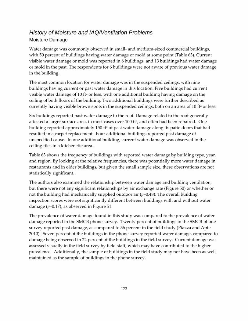
History of Moisture and IAQ/Ventilation Problems Moisture Damage

Water damage was commonly observed in small‐ and medium‐sized commercial buildings, with 50 percent of buildings having water damage or mold at some point (Table 63). Current visible water damage or mold was reported in 8 buildings, and 13 buildings had water damage or mold in the past. The respondents for 6 buildings were not aware of previous water damage in the building.  

The most common location for water damage was in the suspended ceilings, with nine buildings having current or past water damage in this location. Five buildings had current visible water damage of 10 ft2 or less, with one additional building having damage on the ceiling of both floors of the building. Two additional buildings were further described as currently having visible brown spots in the suspended ceilings, both on an area of 10 ft2 or less.  

Six buildings reported past water damage to the roof. Damage related to the roof generally affected a larger surface area, in most cases over 100 ft2, and often had been repaired.  One building reported approximately 150 ft2 of past water damage along its patio doors that had resulted in a carpet replacement.  Four additional buildings reported past damage of unspecified cause.  In one additional building, current water damage was observed in the ceiling tiles in a kitchenette area. 

Table 63 shows the frequency of buildings with reported water damage by building type, year, and region. By looking at the relative frequencies, there was potentially more water damage in restaurants and in older buildings, but given the small sample size, these observations are not statistically significant.  

The authors also examined the relationship between water damage and building ventilation, but there were not any significant relationships by air exchange rate (Figure 50) or whether or not the building had mechanically supplied outdoor air (p=0.48). The overall building inspection scores were not significantly different between buildings with and without water damage (p=0.17), as observed in Figure 51. 

The prevalence of water damage found in this study was compared to the prevalence of water damage reported in the SMCB phone survey.  Twenty percent of buildings in the SMCB phone survey reported past damage, as compared to 36 percent in the field study (Piazza and Apte 2010).  Seven percent of the buildings in the phone survey reported water damage, compared to damage being observed in 22 percent of the buildings in the field survey.  Current damage was assessed visually in the field survey by field staff, which may have contributed to the higher prevalence.  Additionally, the sample of buildings in the field study may not have been as well maintained as the sample of buildings in the phone survey.  

172 

 

 

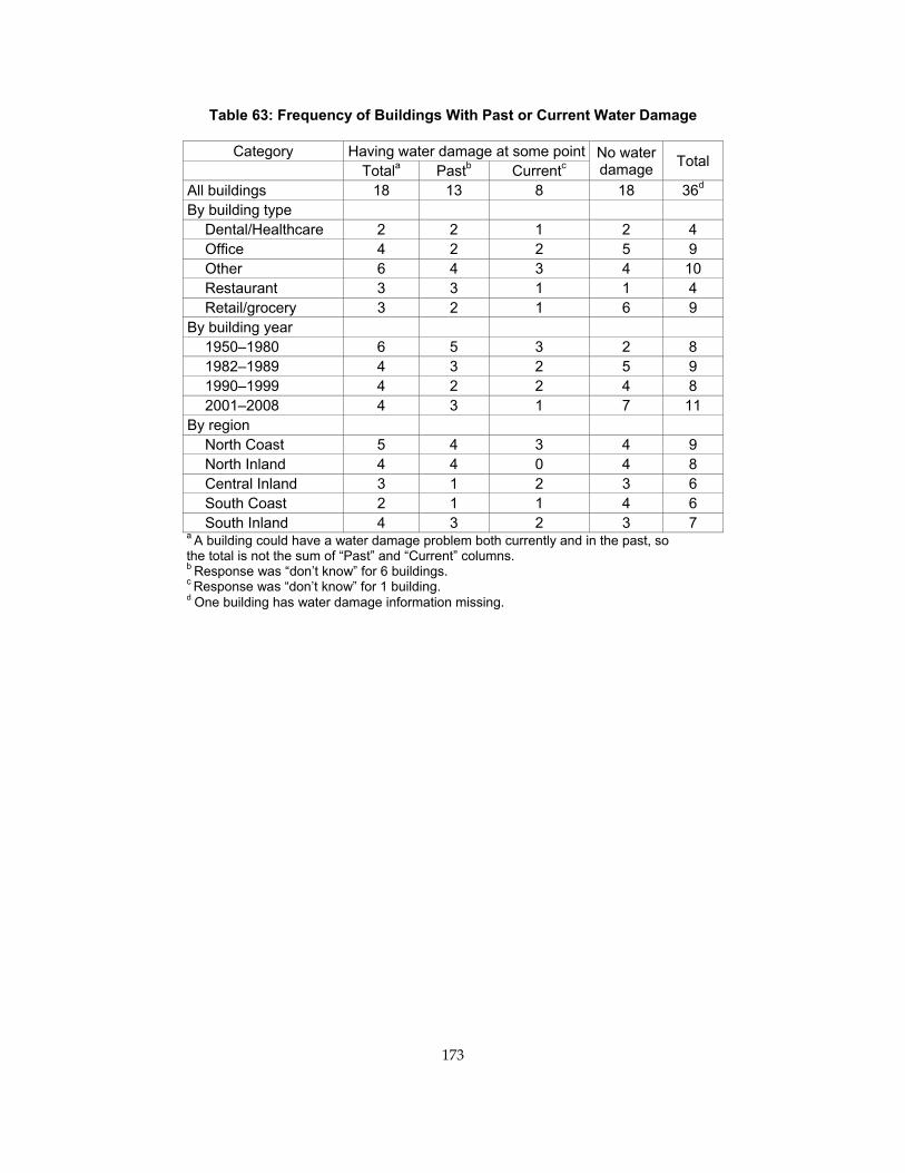
Table 63: Frequency of Buildings With Past or Current Water Damage

Category Having water damage at some point No water damage Total Totala Pastb Currentc

All buildings 18 13 8 18 36d By building type

Dental/Healthcare 2 2 1 2 4 Office 4 2 2 5 9 Other 6 4 3 4 10 Restaurant 3 3 1 1 4 Retail/grocery 3 2 1 6 9

By building year 1950–1980 6 5 3 2 8 1982–1989 4 3 2 5 9 1990–1999 4 2 2 4 8 2001–2008 4 3 1 7 11

By region North Coast 5 4 3 4 9 North Inland 4 4 0 4 8 Central Inland 3 1 2 3 6 South Coast 2 1 1 4 6 South Inland 4 3 2 3 7

a A building could have a water damage problem both currently and in the past, so the total is not the sum of “Past” and “Current” columns. b Response was “don’t know” for 6 buildings. c Response was “don’t know” for 1 building. d One building has water damage information missing. 

 

 

 

 

 

 

 

 

 

 

173 

 

 

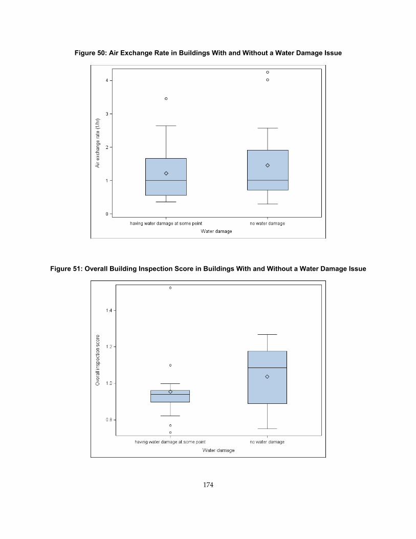
Figure 50: Air Exchange Rate in Buildings With and Without a Water Damage Issue

 

Figure 51: Overall Building Inspection Score in Buildings With and Without a Water Damage Issue

 

174 

 

 

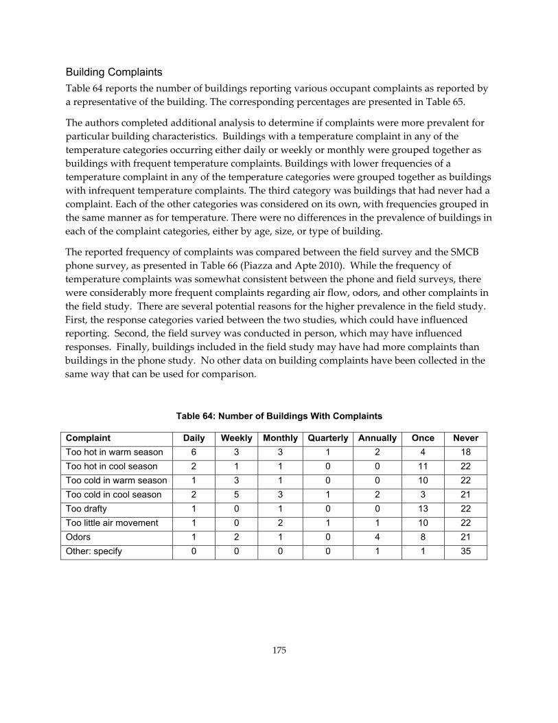
Building Complaints Table 64 reports the number of buildings reporting various occupant complaints as reported by a representative of the building. The corresponding percentages are presented in Table 65. 

The authors completed additional analysis to determine if complaints were more prevalent for particular building characteristics.  Buildings with a temperature complaint in any of the temperature categories occurring either daily or weekly or monthly were grouped together as buildings with frequent temperature complaints. Buildings with lower frequencies of a temperature complaint in any of the temperature categories were grouped together as buildings with infrequent temperature complaints. The third category was buildings that had never had a complaint. Each of the other categories was considered on its own, with frequencies grouped in the same manner as for temperature. There were no differences in the prevalence of buildings in each of the complaint categories, either by age, size, or type of building. 

The reported frequency of complaints was compared between the field survey and the SMCB phone survey, as presented in Table 66 (Piazza and Apte 2010).  While the frequency of temperature complaints was somewhat consistent between the phone and field surveys, there were considerably more frequent complaints regarding air flow, odors, and other complaints in the field study.  There are several potential reasons for the higher prevalence in the field study.  First, the response categories varied between the two studies, which could have influenced reporting.  Second, the field survey was conducted in person, which may have influenced responses.  Finally, buildings included in the field study may have had more complaints than buildings in the phone study.  No other data on building complaints have been collected in the same way that can be used for comparison.   

 

Table 64: Number of Buildings With Complaints

Complaint Daily Weekly Monthly Quarterly Annually Once Never Too hot in warm season 6 3 3 1 2 4 18 Too hot in cool season 2 1 1 0 0 11 22 Too cold in warm season 1 3 1 0 0 10 22 Too cold in cool season 2 5 3 1 2 3 21 Too drafty 1 0 1 0 0 13 22 Too little air movement 1 0 2 1 1 10 22 Odors 1 2 1 0 4 8 21 Other: specify 0 0 0 0 1 1 35

 

175 

 

 

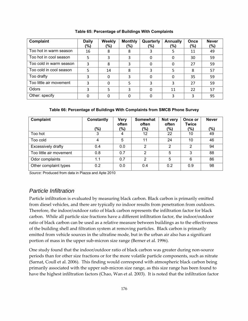
Table 65: Percentage of Buildings With Complaints

Complaint Daily (%)

Weekly(%)

Monthly(%)

Quarterly(%)

Annually (%)

Once (%)

Never (%)

Too hot in warm season 16  8  8  3  5  11  49 Too hot in cool season 5  3  3  0  0  30  59 Too cold in warm season 3  8  3  0  0  27  59 Too cold in cool season 5  14  8  3  5  8  57 Too drafty 3  0  3  0  0  35  59 Too little air movement 3  0  5  3  3  27  59 Odors 3  5  3  0  11  22  57 Other: specify 0  0  0  0  3  3  95 

Table 66: Percentage of Buildings With Complaints from SMCB Phone Survey

Complaint Constantly

(%)

Very often (%)

Somewhat often (%)

Not very often (%)

Once or Twice

(%)

Never

(%) Too hot 3 4 12 22 10 49 Too cold 4 5 11 24 10 46 Excessively drafty 0.4 0.0 2 2 2 94 Too little air movement 0.8 0.7 2 5 3 88 Odor complaints 1.1 0.7 2 5 6 86 Other complaint types 0.2 0.0 0.4 0.2 0.9 98

Source: Produced from data in Piazza and Apte 2010

 

Particle Infiltration Particle infiltration is evaluated by measuring black carbon. Black carbon is primarily emitted from diesel vehicles, and there are typically no indoor results from penetration from outdoors.  Therefore, the indoor/outdoor ratio of black carbon represents the infiltration factor for black carbon.  While all particle size fractions have a different infiltration factor, the indoor/outdoor ratio of black carbon can be used as a relative measure between buildings as to the effectiveness of the building shell and filtration system at removing particles.  Black carbon is primarily emitted from vehicle sources in the ultrafine mode, but in the urban air also has a significant portion of mass in the upper sub‐micron size range (Berner et al. 1996).   

One study found that the indoor/outdoor ratio of black carbon was greater during non‐source periods than for other size fractions or for the more volatile particle components, such as nitrate (Sarnat, Coull et al. 2006).  This finding would correspond with atmospheric black carbon being primarily associated with the upper sub‐micron size range, as this size range has been found to have the highest infiltration factors (Chao, Wan et al. 2003).  It is noted that the infiltration factor 

176 

 

 

as estimated by the indoor/outdoor ratio likely overestimates the infiltration factor for many size fractions.   

The research team used three Aethalometers (one indoors, one on the roof, and one outdoors at street level) to measure black carbon.  Concentrations were recorded every five minutes.  Negative values were removed from the dataset.  Data were averaged over a 30‐minute period, including all available data.  If data from one time period were missing, concentrations were calculated based on the average concentrations for the remaining time periods.  If more than one data point was missing, concentrations were interpolated between the levels estimated just before and just after the period where data were not recorded.  The resulting time series for each building is presented in Appendix H.  If interpolation was done for more than 15 minutes, it is noted below the plot of the time series.   

Theoretically, indoor black carbon concentration measured at a time point corresponds to the outdoor concentration measured some time ago, as particles remain in the air for some time after entering the building. In other words, a concentration peak that occurred outdoors may be observed indoors at a later time. Therefore, besides calculating the indoor/outdoor ratio based on simultaneous indoor and outdoor measurements, the authors also calculated ratios based on outdoor measurement and indoor measurements with delay of 10, 20, and 50 percent of the average age of air in the building. Ratios calculated with a delay between outdoor and indoor concentrations might provide more accurate infiltration estimation. Theoretically, the infiltration factor should be fairly constant throughout the day.  The distribution of the calculated indoor/outdoor ratio for each building was calculated, and the time lag that resulted in the smallest standard deviations was used, as this time lag resulted in the most stable estimate of the infiltration factor as represented by the indoor/outdoor ratio.   

To represent outdoor black carbon concentrations, the research team collected samples, both on the roof and at street level. To determine which measurement should be used in calculating indoor/outdoor ratios, the following decision rule was created:  If the mechanically delivered outdoor air of a building was more than 50 percent of the whole‐building ventilation rate, namely the majority of outdoor air coming from the rooftop unit, the measurement on the roof was used as the denominator. Otherwise, the measurement at street level was used as the denominator. 

The authors observed an indoor/outdoor ratio larger than 1 in a few buildings, including two hair salons, one dental office, a bookstore, and a fleet service office. Since the origin of black carbon is primarily outdoors, values over 1 indicate that the indoor/outdoor ratio of black carbon as a representation of particle infiltration has limitations  in these buildings. Ratios greater than 1 may result from indoor sources, either direct sources or resuspension, as a result of measurement error, or due to the assumptions for using the indoor/outdoor black carbon as a measure of infiltration not being met.  Specifically, it is assumed that the outdoor measure of black carbon represents the air concentration of all air infiltrating the buildings, which may not be the case if levels are variable from one side of the building to the other, which could result if there is more vehicle traffic on one side than the other.  Second, it is assumed that measured 

177 

 

 

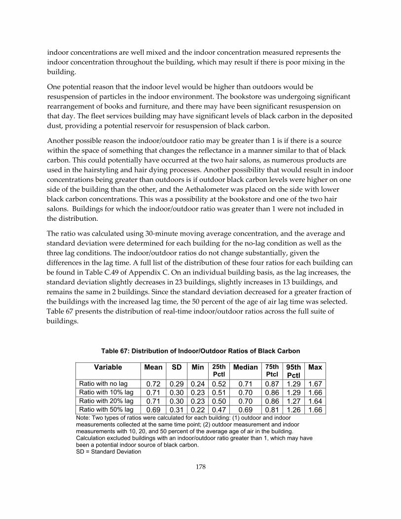
indoor concentrations are well mixed and the indoor concentration measured represents the indoor concentration throughout the building, which may result if there is poor mixing in the building. 

One potential reason that the indoor level would be higher than outdoors would be resuspension of particles in the indoor environment. The bookstore was undergoing significant rearrangement of books and furniture, and there may have been significant resuspension on that day. The fleet services building may have significant levels of black carbon in the deposited dust, providing a potential reservoir for resuspension of black carbon.  

Another possible reason the indoor/outdoor ratio may be greater than 1 is if there is a source within the space of something that changes the reflectance in a manner similar to that of black carbon. This could potentially have occurred at the two hair salons, as numerous products are used in the hairstyling and hair dying processes. Another possibility that would result in indoor concentrations being greater than outdoors is if outdoor black carbon levels were higher on one side of the building than the other, and the Aethalometer was placed on the side with lower black carbon concentrations. This was a possibility at the bookstore and one of the two hair salons.  Buildings for which the indoor/outdoor ratio was greater than 1 were not included in the distribution. 

The ratio was calculated using 30‐minute moving average concentration, and the average and standard deviation were determined for each building for the no‐lag condition as well as the three lag conditions. The indoor/outdoor ratios do not change substantially, given the differences in the lag time. A full list of the distribution of these four ratios for each building can be found in Table C.49 of Appendix C. On an individual building basis, as the lag increases, the standard deviation slightly decreases in 23 buildings, slightly increases in 13 buildings, and remains the same in 2 buildings. Since the standard deviation decreased for a greater fraction of the buildings with the increased lag time, the 50 percent of the age of air lag time was selected.  Table 67 presents the distribution of real‐time indoor/outdoor ratios across the full suite of buildings. 

 

Table 67: Distribution of Indoor/Outdoor Ratios of Black Carbon

Variable Mean SD Min 25th Pctl

Median 75th Ptcl

95th Pctl

Max

Ratio with no lag 0.72 0.29 0.24 0.52 0.71 0.87 1.29 1.67 Ratio with 10% lag 0.71 0.30 0.23 0.51 0.70 0.86 1.29 1.66 Ratio with 20% lag 0.71 0.30 0.23 0.50 0.70 0.86 1.27 1.64 Ratio with 50% lag 0.69 0.31 0.22 0.47 0.69 0.81 1.26 1.66

Note: Two types of ratios were calculated for each building: (1) outdoor and indoor measurements collected at the same time point; (2) outdoor measurement and indoor measurements with 10, 20, and 50 percent of the average age of air in the building. Calculation excluded buildings with an indoor/outdoor ratio greater than 1, which may have been a potential indoor source of black carbon. SD = Standard Deviation 

178 

 

 

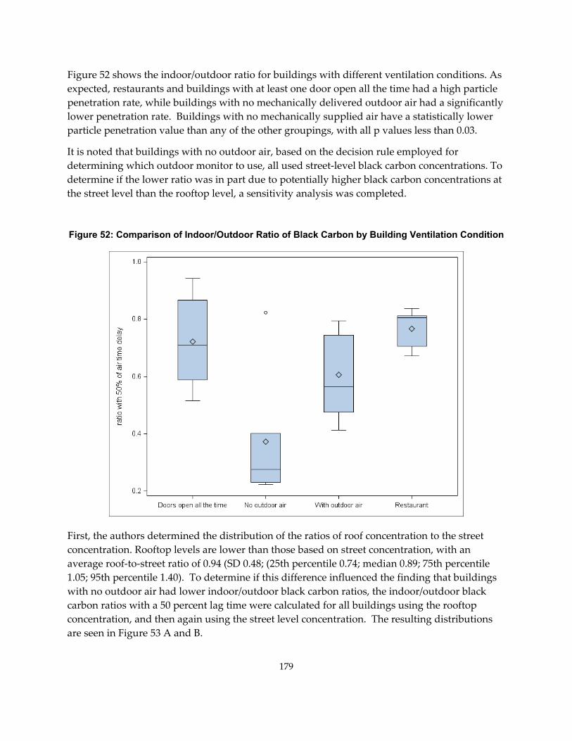
Figure 52 shows the indoor/outdoor ratio for buildings with different ventilation conditions. As expected, restaurants and buildings with at least one door open all the time had a high particle penetration rate, while buildings with no mechanically delivered outdoor air had a significantly lower penetration rate.  Buildings with no mechanically supplied air have a statistically lower particle penetration value than any of the other groupings, with all p values less than 0.03. 

It is noted that buildings with no outdoor air, based on the decision rule employed for determining which outdoor monitor to use, all used street‐level black carbon concentrations. To determine if the lower ratio was in part due to potentially higher black carbon concentrations at the street level than the rooftop level, a sensitivity analysis was completed. 

Figure 52: Comparison of Indoor/Outdoor Ratio of Black Carbon by Building Ventilation Condition 

 

First, the authors determined the distribution of the ratios of roof concentration to the street concentration. Rooftop levels are lower than those based on street concentration, with an average roof‐to‐street ratio of 0.94 (SD 0.48; (25th percentile 0.74; median 0.89; 75th percentile 1.05; 95th percentile 1.40).  To determine if this difference influenced the finding that buildings with no outdoor air had lower indoor/outdoor black carbon ratios, the indoor/outdoor black carbon ratios with a 50 percent lag time were calculated for all buildings using the rooftop concentration, and then again using the street level concentration.  The resulting distributions are seen in Figure 53 A and B. 

179 

 

 

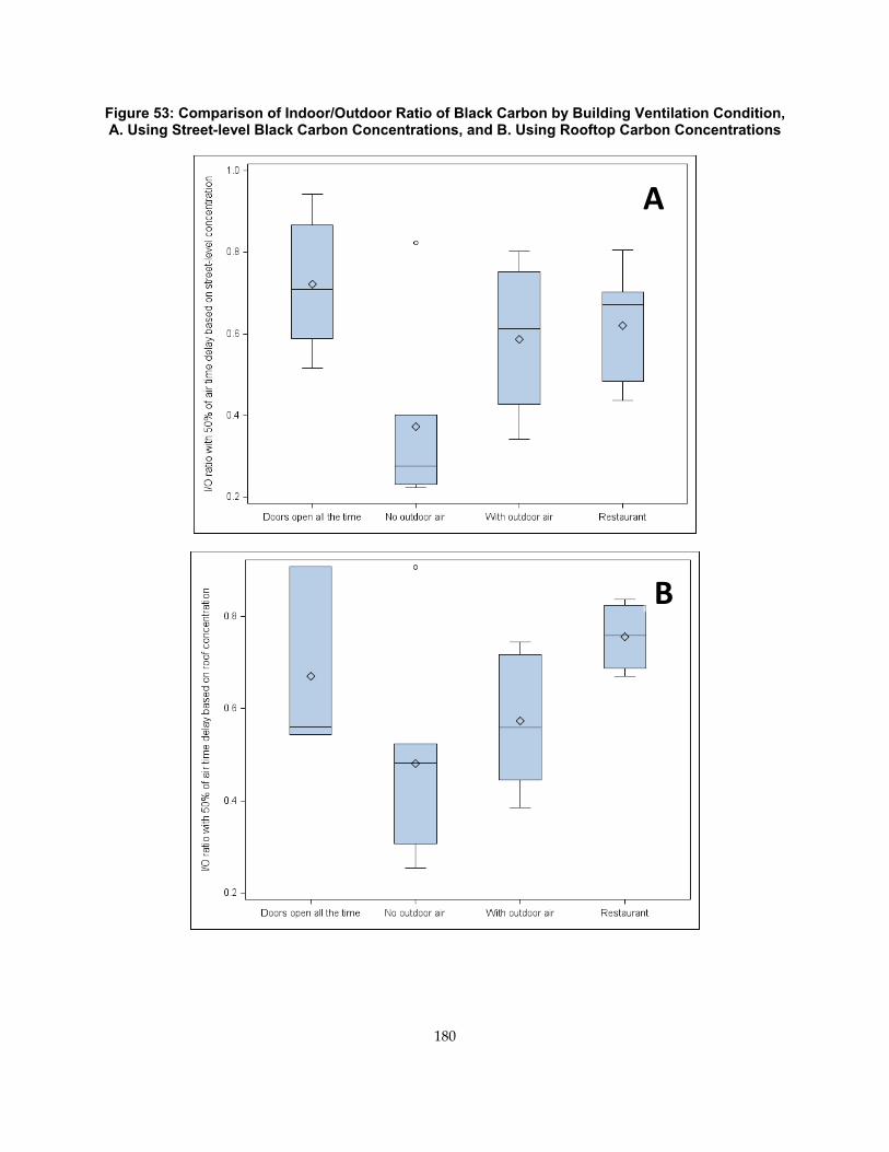
Figure 53: Comparison of Indoor/Outdoor Ratio of Black Carbon by Building Ventilation Condition, A. Using Street-level Black Carbon Concentrations, and B. Using Rooftop Carbon Concentrations 

 

A 

 

B 

180 

 

 

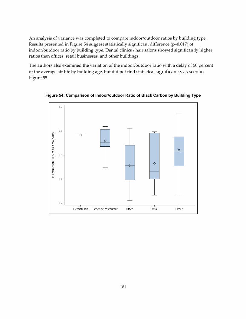
 An analysis of variance was completed to compare indoor/outdoor ratios by building type. Results presented in Figure 54 suggest statistically significant difference (p=0.017) of indoor/outdoor ratio by building type. Dental clinics / hair salons showed significantly higher ratios than offices, retail businesses, and other buildings.   

The authors also examined the variation of the indoor/outdoor ratio with a delay of 50 percent of the average air life by building age, but did not find statistical significance, as seen in Figure 55.  

 

Figure 54: Comparison of Indoor/outdoor Ratio of Black Carbon by Building Type 

 

 

181 

 

 

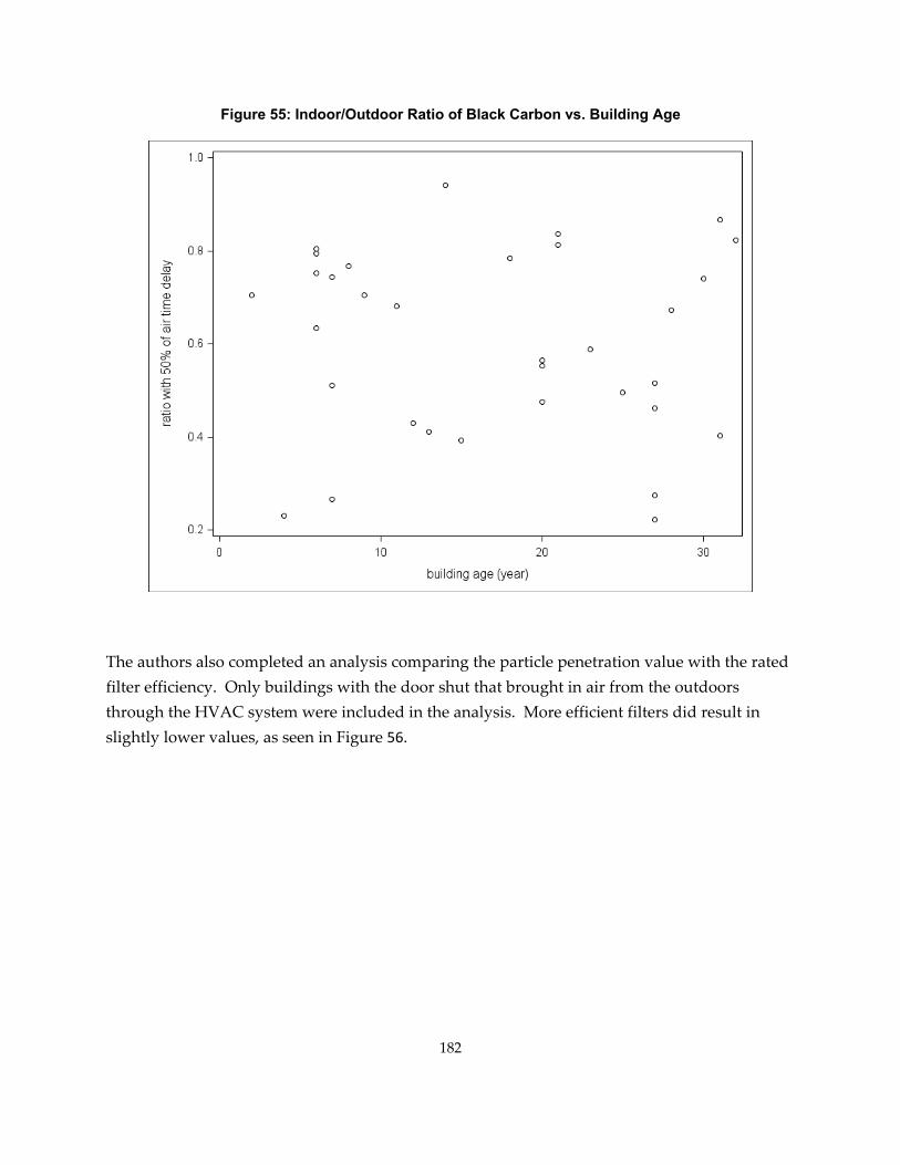
Figure 55: Indoor/Outdoor Ratio of Black Carbon vs. Building Age

 

The authors also completed an analysis comparing the particle penetration value with the rated filter efficiency.  Only buildings with the door shut that brought in air from the outdoors through the HVAC system were included in the analysis.  More efficient filters did result in slightly lower values, as seen in Figure 56. 

182 

 

 

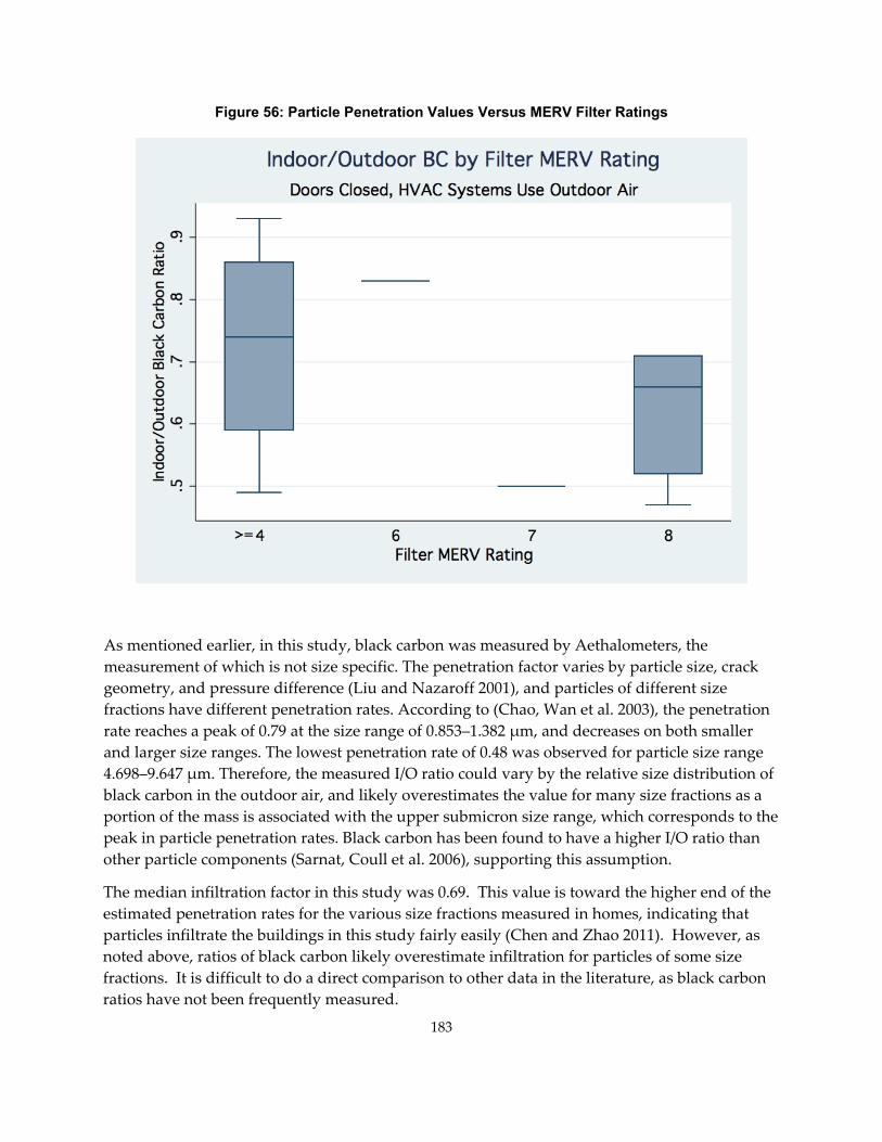
Figure 56: Particle Penetration Values Versus MERV Filter Ratings

 

 

As mentioned earlier, in this study, black carbon was measured by Aethalometers, the measurement of which is not size specific. The penetration factor varies by particle size, crack geometry, and pressure difference (Liu and Nazaroff 2001), and particles of different size fractions have different penetration rates. According to (Chao, Wan et al. 2003), the penetration rate reaches a peak of 0.79 at the size range of 0.853–1.382 μm, and decreases on both smaller and larger size ranges. The lowest penetration rate of 0.48 was observed for particle size range 4.698–9.647 μm. Therefore, the measured I/O ratio could vary by the relative size distribution of black carbon in the outdoor air, and likely overestimates the value for many size fractions as a portion of the mass is associated with the upper submicron size range, which corresponds to the peak in particle penetration rates. Black carbon has been found to have a higher I/O ratio than other particle components (Sarnat, Coull et al. 2006), supporting this assumption. 

The median infiltration factor in this study was 0.69.  This value is toward the higher end of the estimated penetration rates for the various size fractions measured in homes, indicating that particles infiltrate the buildings in this study fairly easily (Chen and Zhao 2011).  However, as noted above, ratios of black carbon likely overestimate infiltration for particles of some size fractions.  It is difficult to do a direct comparison to other data in the literature, as black carbon ratios have not been frequently measured. 

183 

 

 

 

It is noted that outdoor black carbon concentrations can also be used as a proxy for exposure to air pollution from traffic, and the indoor concentrations can be used to evaluate the impact of vehicle pollution sources on the indoor environment; however, this is beyond the scope of this project.   

QA/QC Results for Aethalometers To test the three Aethalometers used in the field sampling, the research team conducted three co‐location tests during the study. The authors compared both original count reading and the 30‐minute moving average count among the three instruments. AE3 was the newest instrument among the three, and considered the most reliable. The reading of AE1 fairly agreed with AE3, while AE2 consistently underestimated the black carbon concentration as compared to AE3. Based on 30‐minute moving average count of the three tests, we summarized the following conversion equations to correct the data collected by AE1 and AE2. 

For AE1:   AE1’ = 1.2391 * AE1 – 21.707  R2=0.9739 

For AE2:   AE2’ = 1.4652 * AE2 – 6.4981  R2=0.9114 

184 

 

 

CHAPTER 4: Conclusions and Recommendations Conclusions  Small‐ and medium‐sized commercial buildings make up 96 percent of the commercial buildings in the United States, using nearly 18 percent of the country’s energy supply.  California’s commercial sector compressor‐based cooling constitutes roughly 15 percent of total electricity consumption, and total energy use in commercial buildings represented 10.8 percent of total statewide greenhouse gas emissions in 2008. These buildings also serve as a place of work for a number of Californians, and thus the air quality in these buildings is important to understand.  The research team conducted a field study of approximately 40 small‐ and medium‐sized commercial buildings (SMCBs with floor area between 1,000 and 50,000 ft2 and with fewer than four stories).  The primary goals were to obtain information on the ventilation of the buildings and on the sources of air pollutants in the buildings. 

The majority of the buildings were built from 1978 to 2006.  There was an approximately even distribution of buildings from each of five regions of the state: North‐Coastal, North‐Inland, South‐Coastal, South‐Inland, and Central‐Inland.  The buildings varied in their function, with the sample including seven retail establishments, five restaurants, eight offices, and two each of gas stations, hair salons, healthcare facilities, grocery store, dental offices, and gyms—along with five other buildings.  The buildings were primarily recruited as a random sample, with some of the difficult building types a convenience sample.  

This is the most comprehensive study of ventilation and air quality in SMCB.  Previous studies have either focused on factors such as building use and energy use (Itron Inc. 2006) or exclusively of HVAC function (Cummings, Withers et al. 1996).  Both ventilation and indoor air quality were extensively evaluated in primarily large commercial buildings as part of the BASE study (Girman, Hadwen et al. 1999; Apte, Fisk et al. 2000; Environmental Health and Engineering 2002; U.S. EPA 2003; Persily and Gorfain 2004; Mendell, Cozen et al. 2006; Apte, Buchanan et al. 2008); however, such a complete evaluation has not been conducted in SMCB of varied use until this study. The following paragraphs present the conclusions for each of the project’s objectives. 

Objective 1: Obtain data on SMCB building characteristics, operation and maintenance of their HVAC, and air filtration systems. The first goal of the project was to obtain information available from an inspection of the HVAC system.  The research team found that 16 buildings did not have mechanically supplied outdoor air, including all the buildings built prior to 1980, but also 19 percent of the buildings built since 1980.  In these cases, the air handling unit was generally not a commercial model.  This finding was rather surprising.  It is noted that this study had a relatively small sample size and thus these findings should be confirmed by conducting a larger study. Additionally, it is not clear if the building sample is completely representative, or if it included a higher portion of buildings that may not have had sophisticated and well‐maintained systems.  When the research team 

185 

 

 

contacted buildings that housed a facility that was part of a national chain, there was generally a lack of willingness to have the buildings be part of the study.  Therefore, without a larger sample size, it is difficult to know if this finding is representative for this type of building. Even if the statewide prevalence of buildings without mechanically supplied air is lower, it is concerning that any buildings were found not to have mechanically supplied outdoor air, as this is a requirement under Title 24.   

Buildings generally had low‐efficiency filters, with 56 percent having a MERV rating of 4 or lower. This was in stark contrast to the high‐efficiency filters found in the large office buildings in the BASE study. The fact that the penetration efficiency as measured by the black carbon ratio was higher for buildings that brought air in through the mechanically supplied system than it was for buildings bringing in outdoor air through uncontrolled leakage may result from the relatively low filter efficiencies. The authors observed lower particle penetration efficiencies in buildings with higher‐efficiency filters, demonstrating the benefit of these filters.  It is noted, however, that for the most part, buildings did not have unacceptable levels of particulate matter as a result of these low‐efficiency filters.  Additionally, the inspection revealed that the filters were sometimes in poor condition, and in some cases very worn or not properly installed.  While only a couple of buildings did not have accessible filters, the condition of the filters in systems with poor access was (statistically) significantly poorer. 

Only a quarter of the buildings had a contractor that regularly inspected the HVAC system.  Buildings with regular HVAC contractor visits had HVAC systems that were in better condition. Conditions were mixed, with smaller buildings having less well‐maintained systems.  Again, the authors note that the buildings in this sample may not have been as well maintained as the distribution of buildings across the State.  The SMCB phone survey found a much higher proportion of buildings having regular inspections.  However, the information on maintenance was not obtained over the phone interview, but rather from the mail‐in survey.  Such willing respondents were likely to be more conscientious building managers, and therefore may also not be representative of the distribution of the building stock.  This selection bias may cause an overestimation of the portion of buildings receiving regular inspections. One of the analyses of the BASE study found that poor maintenance of the HVAC systems was associated with symptoms consistent with sick building syndrome (Mendell, Lei‐Gomez et al. 2008), highlighting the need for more frequent inspection and maintenance of HVAC systems in SMCB. 

Objective 2: Recognizing that measurement of air flow can be problematic, field data on the design and performance parameters of HVAC and air filtration systems in SMCB were to be obtained. The second goal was to measure the air exchange rates and amount of outdoor mechanically supplied air delivered to buildings.  To meet this objective, the research team determined the overall air exchange rate by a steady‐state method using a continuous emission of a perfluorocarbon tracer and with a tracer decay method, using a sulfur hexafluoride tracer. The research team also calculated overall air exchange using a CO2 equilibrium method.   

186 

 

 

As three methods were used to measure whole‐building air exchange, the authors completed an evaluation to determine the most effective among them.  The tracer decay method generally resulted in slightly higher values than the steady‐state perfluorocarbon tracer (PFT) method, likely because it was a measure of the air exchange during the occupied period, while the PFT was also influenced by the nighttime period, which likely had a lower air exchange rate, as the spaces were not occupied then.  The investigators found that the CO2 equilibrium method was not effective in many buildings due to low or inconsistent occupancy, while the tracer decay method provided the best reflection of ventilation during occupied periods. The Spearman correlation coefficient between the tracer decay and the equilibrium methods was 0.78, indicating that if it is not possible to conduct tracer decay measurements, the steady‐state method will provide a reasonable method for comparing buildings. These findings may be instructive for future studies. 

The supply of outside air was 0.27 with a standard deviation of 0.27 cfm/ft2 (or an air exchange rate of 1.6 with a standard deviation of 1.7 h‐1).  On a per‐area basis, this value is considerably less than the 1.0 cfm/ft2 that was measured in the BASE study, although the building occupancy was likely greater in the buildings evaluated in the BASE study (Persily and Gorfain 2004).   

Overall air exchange rates were similar between buildings with and without mechanically supplied outdoor air, indicating that uncontrolled leakage served to provide ventilation despite a lack of mechanical introduction.  This finding suggests that better management of building tightness and ventilation may also be an avenue for energy conservation.  However, the authors note that based on indoor air quality, it would be important to focus on source reduction prior to conducting efforts to limit air exchange.  Seven buildings kept doors open all the time, and for these naturally ventilated buildings, the air exchange rates were higher.  Restaurants had higher air exchange rates than other building types.  There were no other differences in air exchange rates by building use, size, or age. 

Where possible, the research team measured the outdoor air supply rate.  For the 23 buildings for which mechanically supplied outdoor air could be measured, the ratio of the mechanically supplied outdoor air to the overall air supply was determined.  For nine buildings it was estimated that all air was mechanically supplied, although the mechanically supplied air was likely overestimated due to measurement methods.  For the remaining buildings, on average, 45 percent of the outdoor air was mechanically supplied.  It is noted that in many cases, the buildings did not run the HVAC unit all the time, therefore the Duct Blaster measurements imply the maximum possible airflow but may not be the actual flow on that day.  Only two of the buildings reported having used an economizer cycle that influenced ventilation on the majority of occupants.  For these two reasons the actual contribution of mechanically supplied outdoor air to total supplied outdoor air may be overestimated in many of the buildings. 

The majority of the buildings met the outside air ventilation rates required in Title 24 on a per‐person basis. However, when comparing to their ventilation rates to those required in Title 24 by area, healthcare establishments, gyms, offices, hair salons, and retail businesses all ventilated below the standard, while restaurants and gas stations had exchange rates significantly higher 

187 

 

 

than the standard. Grocery stores, dental offices, and other building types have values close to the Title 24 required value. It is noted that the methods used for measuring air flow in this study in restaurants include flow that results from the exhaust hoods in the kitchen that is required under additional building code statutes.  Exhaust hoods require makeup air that increases ventilation in the space.  In the small buildings that were studied there was typically little physical separation between the kitchen and dining areas; thus, measured ventilation rates were strongly influenced by the kitchen hood flows. 

There are only limited previous studies to which air exchange rates can be compared.  When compared to the air exchange rates measured in the BASE study, the air exchange rates measured in this study are quite low (P&G 2004).  Almost all of the buildings in the BASE study met the ASHRAE 62.1 standard, in stark contrast to the high percentages of buildings in this study that did not meet the air exchange standard.  A study of small commercial buildings in central Florida measured air exchange rates that were also relatively low, and consistent with those measured in this study (Cummings 1996).  The previous study noted the lack of care in designing HVAC systems in small buildings—a finding echoed in this study.  This finding suggests a need for a more comprehensive permitting and inspection process, such as the process that is required for large commercial buildings. 

There were only a limited number of buildings that exceeded the implied CO2 concentrations in the ventilation standards. These buildings (including a gym, hair salon, office buildings, and restaurant) all generally had high occupancy. 

Objective 3: Obtain data on indoor pollutant levels, especially toxic air contaminants, and potential pollutant sources in a variety of SMCB. To the extent feasible, determine the moisture-related history and IAQ complaint history. One goal was to obtain information on indoor pollutant levels and to determine if the measured levels were a result of indoor sources.  The research team made real‐time carbon monoxide measurements, and levels of this compound were found to be below regulatory levels.  The research team also made real‐time measurements for both ultrafine particulate matter (PM) and PM between 0.3 and 5 μm and integrated PM10 and PM2.5, both inside and outside of each building.  The majority of the buildings had indoor/outdoor ratios less than 1.0 for both ultrafine and PM 2.5.  However, some of the buildings had clear indications of indoor PM sources with higher indoor levels than outdoor levels; particularly restaurants, hair salons, and dental offices. 

This study measured a suite of 30 aldehydes and VOCs indoors and outdoors for approximately four hours.  The geometric mean (± geometric standard deviation) indoor concentrations for some of the traditionally measured compounds include 0.7±1.6 μg/m3 for benzene, 4.5±3.6 μg/m3 for toluene, 16±2.3μg/m3 for formaldehyde, and 8.9±2.5μg/m3 for acetaldehyde.  The study also included compounds only more recently measured in indoor spaces, reported as median / 95th percentile values, such as 2‐butoxy ethanol (3.6 / 241 μg/m3), d‐limonene 

188 

 

 

(8.3 / 239 μg/m3), TXIB (1.0 / 5.8 μg/m3), and D5‐siloxane (26 / 120 μg/m3).  There was a considerable range in the actual concentrations for each of the contaminants, with 27 of the compounds having an extremely high concentration (at least five times the standard deviation) in at least one building.  

For 10 of the compounds, there were significant differences in the indoor concentrations by building type.  The building types with higher concentrations were generally expected; for example, chloroform was higher in restaurants and groceries; diethylphthalate was higher in dental offices, healthcare establishments, hair salons, and gyms; and m/p‐xylene was higher at gas stations.   

The investigators completed a factor analysis and found several factors to be important. Factor 1 represents outdoor sources, with high loadings of benzene, toluene, ethylbenzene and xylenes (BTEX), and n‐hexane, primarily emitted from automatable sources. Factor 2 includes high loadings of d‐limonene, α‐terpineol, and D5‐siloxane, which are related to cleaning products. Factor 3 represents high molecular weight aldehydes, and Factor 5 represents low molecular weight aldehydes. Factor 4 has high loadings of TXIB and diethylphthalate, which are plasticizers.  

The majority of buildings had formaldehyde levels above the OEHHA recommended level of 9 μg/m3, and this is a very significant finding.  The percent difference on the formaldehyde samples was 4.4 percent, and thus the authors are quite confident of the formaldehyde measures made in this study.  A comparison to the BASE study indicated that indoor formaldehyde concentrations were higher in this study, either because levels are higher in SMCB as compared to large office buildings, or because formaldehyde emission rates in buildings materials, furnishings, and consumer products has increased in the time period between these two studies.  A further analysis to determine the formaldehyde levels that would exist had the buildings exactly met ventilation requirements under Title 24 were determined, and in all cases except gas stations was completed. The resulting formaldehyde levels exceeded the OEHHA recommended levels.  This finding indicates that increasing ventilation is not an adequate method to reduce concentrations, but rather source reduction is necessary. Source reduction would require changes in building products, furnishings, and consumer products sold in this State.   

The research team asked building managers for any record they have on the history of both moisture and IAQ complaints in the buildings.  Most complaints were temperature related.  There were frequent reports of water damage, but in most cases, it had either been repaired or was not extensive. 

Objective 4: Measure particulate matter inside and outside of buildings, to estimate penetration rates for particulate matter in a variety of SMCB. Inside and outside Aethalometers were run to determine the level of black carbon.  Because black carbon is primarily a compound of outdoor origin, these levels may be used to determine the fraction of outdoor particles penetrating indoors and staying airborne, considering 

189 

 

 

deposition and filtration losses.  The average penetration rates as measured by black carbon instruments was 0.72.  Surprisingly, but possibly consistent with the observed high prevalence of HVAC filters of very low efficiency, buildings with no mechanically supplied outdoor air had lower penetration rates compared against buildings with mechanically supplied outdoor air.  

Recommendations The key findings from this study are: (1) current Title 24 codes for HVAC equipment and mechanical ventilation appear to not always be enforced, resulting in a lack of mechanically supplied outdoor air, (2) some buildings have very limited or no maintenance conducted on their heating, ventilation, and air‐conditioning units, (3) California commercial buildings have significant uncontrolled leakage—a condition that has been addressed in California homes in recent years (Offermann 2009), (4) indoor levels of most pollutants are below regulatory or recommended health protective levels, with the notable exception of formaldehyde, which was consistently found to exceed the OEHHA chronic reference exposure level, and (5) particle filters are generally of low efficiency.  

One impetus for this study was a concern over a lack of information on how California buildings are being ventilated and the extent to which indoor contaminant sources contribute to compromised indoor air quality.  Another concern was a similar lack of information on the impact of building design and operation practices on energy consumption, particularly related to ventilation, heating, and cooling.  There is no organized mechanism in place to collect this information.  The observations in this study have shown that these concerns are well founded. 

The recommendations stem from these key findings. 

Inspection Procedure and Maintenance The first major recommendation is that the building inspection procedure should include a determination of whether the heating, ventilation, and air‐conditioning units meet the Title 24 requirement for mechanically supplied outdoor air at the required rate (excepting the case where the natural ventilation option can be demonstrated through a code check and inspection to meet the same ventilation rates). This could best be accomplished by adding an inspection of the HVAC unit to the required elements of the required inspection associated with finalizing the building permit.  In some cases, it was clear that noncommercial HVAC units were installed in commercial buildings. Improved labeling of equipment might limit this problem.  However, specific packaging and labeling requirements for California requirements may be burdensome for manufacturers with markets in other states. 

Another possible mechanism for improving compliance would be to require that an HVAC contractor complete a test and balance procedure that included a certification of mechanically supplied outdoor airflow rate.  Building inspectors doing the commissioning of buildings would inspect a small percentage, for example 5 percent, of buildings to confirm that the measured flow rate as declared by the HVAC contractor was the actual measured mechanically supplied outdoor air flow rate. If the value declared by the contractor was not accurate within a 

190 

 

 

specified range, a system of warnings and eventually consequences would be invoked. Additionally, during the inspection, the inspector would confirm that filters are accessible. 

Another major finding was that most buildings do not have an annual inspection and maintenance of their HVAC equipment.  One recommendation that results from this finding is that ideally, some sort of annual maintenance and inspection should be required.  This could be enforced by a requirement for an annual inspection certified by a letter from a licensed HVAC inspector.  Ideally, this process should be set up to be recorded electronically. 

All buildings inspected that were built prior to 1978 did not have mechanically supplied outdoor air.  To address this, one recommendation would be to require buildings be brought up date in the current Title 24 standards at change of ownership.  This would include such factors as the requirement that ventilation units provide mechanically supplied outdoor air.  One may even want to consider bringing buildings up to Title 24 standards when a new lease is signed. 

Building operators appear to have little knowledge in regard to their HVAC system.  It could be useful to provide some instruction to the new building operator at change of ownership or new lease.  One idea might be to introduce a building exchange tax that could then support development of either educational materials or provide free education classes to help operators understand the importance of maintaining an HVAC system.  Ideally, some sort of inspection should be required; however, this is likely not to be cost effective or feasible.  One may even want to consider recommissioning existing buildings at transfer of ownership, requiring that HVAC units be upgraded to include mechanically supplied outdoor air. 

Indoor Air Quality The second major recommendation would be to require lower formaldehyde building source strengths from building materials and other products.  It is clear from the analysis in this study that formaldehyde concentrations are likely to exceed OEHHA recommended levels at Title 24 minimum ventilation standards; either formaldehyde building source strengths need to be decreased or recommended ventilation rates need to increase. Since an increase in the Title 24 recommended ventilation rates is counter to goals of reducing energy consumption, a more appropriate solution would be to require a decrease in formaldehyde building source strengths. An analysis indicated that formaldehyde concentrations were greater in carpeted buildings. This may be one logical starting place for reducing formaldehyde building source strengths, but clearly emissions from other products would need to be considered. We do not have any recommendations on how lower emission products be incorporated into regulation. 

More attention should be paid to development of appropriate formaldehyde air cleaning technologies (Fisk 2008). These might become an appropriate alternative to source reduction. More awareness of additional ventilation during introduction of new products after installation would be beneficial; however, there is no practical way to enforce this.  Given that formaldehyde concentrations already exceed OEHHA levels in the majority of buildings, it would be difficult to recommend increasing building tightness and reducing air exchange rates. 

191 

 

 

The high prevalence of low‐efficiency filters was a surprising finding. While measured particulate matter levels were generally not above regulatory limits, it would still be beneficial to decrease particulate matter levels by increasing the efficiency of filters. It was apparent that there were particulate matter sources in restaurants, hair salons, and dental offices.  These types of buildings, along with other building use is anticipated to have high particulate matter sources, would particularly benefit from the use of higher efficiency filters. Additionally, the outdoor PM2.5 levels were very high for the buildings monitored in the Central Valley of California, as expected.  While the buildings did not have any indoor sources, and had relatively low indoor/outdoor ratios, they still had some of the higher indoor levels of the non‐source buildings in the study sample.  Buildings in areas with typically high outdoor levels would also be good candidates to benefit from the use of higher‐efficiency filters. We recommend creating a requirement for use of higher‐efficiency filters in both building types that are likely to generate significant particulate matter, and buildings in regions with high outdoor levels. It is acknowledged that this recommendation would be difficult to enforce.  It is acknowledged that requiring higher‐efficiency filters would increase costs; however, studies have indicated that higher‐quality filters last longer and require less labor associated with frequency of replacement, negating some of the cost increases (Fisk, Faulkner et al. 2002).  

 

192 

 

 

References 8 CCR 5141. California Code of Regulations, Title 8.“Dusts, Fumes, Mists, Vapors and Gases,” (2011) (Article 107), Control of Hazardous Substances (Group 16), General Industry Safety Orders (Subchapter 7), California Code of Regulations.  

8 CCR 5155. California Code of Regulations, Title 8. “Dusts, Fumes, Mists, Vapors and Gases,” (2011) (Article 107) Appendix Table AC‐1, Control of Hazardous Substances (Group 16), General Industry Safety Orders (Subchapter 7), California Code of Regulations.  

40 CFR 136, Appendix B. Title 40 ‐ Protection of Environment Chapter I ‐ Environmental Protection Agency, Subchapter D ‐ Water Programs, Part 136 ‐ Guidelines Establishing Test Procedures for the Analysis of Pollutants. Appendix B to Part 136 ‐ Definition and Procedure for the Determination of the Method Detection Limit ‐ Revision 1.11.  Accessible at http://ecfr.gpoaccess.gov/cgi/t/text/text‐idx?c=ecfr&tpl=/ecfrbrowse/Title40/40cfr136_main_02.tpl. Click on the ʺAppendix B to Part 136ʺ link. 

Abt, E., H. H. Suh, et al. (2000). ʺCharacterization of indoor particle sources: A study conducted in the metropolitan Boston area.ʺ Environmental Health Perspectives 108(1): 35–44. 

Abt, E., H. H. Suh, et al. (2000). ʺRelative contribution of outdoor and indoor particle sources to indoor concentrations.ʺ Environmental Science & Technology 34(17): 3579–3587. 

Adar, S. D., D. R. Gold, et al. (2007). ʺFocused exposures to airborne traffic particles and heart rate variability in the elderly.ʺ Epidemiology 18(1): 95–103. 

Adgate, J. L., T. R. Church, et al. (2004). ʺOutdoor, indoor, and personal exposure to VOCs in children.ʺ Environmental Health Perspectives 112(14): 1386–1392. 

Adgate, J. L., L. E. Eberly, et al. (2004). ʺPersonal, indoor, and outdoor VOC exposures in a probability sample of children.ʺ Journal of Exposure Analysis and Environmental Epidemiology 14: S4–S13. 

Alevantis, L. (2003). Building Material Emissions Study. Final Report to California Integrated Waste Management Board. 

Allen, J. G., M. D. McClean, et al. (2008). ʺCritical factors in assessing exposure to PBDEs via house dust.ʺ Environment International 34(8): 1085–1091. 

ALNOR (1998). ʺLoFlow Balometer Owners Manual.ʺ ALNOR Instrument Company, Skokie, Illinois. 

Apte, M. G. (2009). ʺResponse to ʹDoes filter media type really affect BRS?ʹ.ʺ Indoor Air 19(6): 526–528. 

Apte, M. G., I. S. H. Buchanan, et al. (2008). ʺOutdoor ozone and building‐related symptoms in 

193 

 

 

the BASE study.ʺ Indoor Air 18(2): 156–170. 

Apte, M. G., and C. A. Erdmann (2002). Associations of Indoor Carbon Dioxide Concentrations, VOCs, and Environmental Susceptibilities with Mucous Membrane and Lower Respiratory Sick Building Syndrome Symptoms in the BASE Study: Analyses of the 100 Building Database. Indoor Enviornment Department, Enviornmental Energy Technologies Division, Lawrence Berkeley National Laboratory. 

Apte, M. G., W. J. Fisk, et al. (2000). ʺAssociations between indoor CO2 concentrations and sick building syndrome symptoms in US office buildings: An analysis of the 1994‐1996 BASE study data.ʺ Indoor Air‐International Journal of Indoor Air Quality and Climate 10(4): 246–257. 

Apte, M. G., B. Norman, et al. (2008). Improving Ventilation and Saving energy: Final Report on Indoor Environmental Quality and Energy Monitoring in Sixteen Relocatable Classrooms. Lawrence Berkeley National Laboratory, Berkeley, California. 

ASHRAE (1998). ASHRAE/ANSI Standard 111‐98 Practices for Measurement, Testing, Adjusting and Balancing of Building Heat Ventilation, Air‐Conditioning and Refrigeration Systems. ASHRAE, Atlanta, Georgia. 

ASHRAE (2002). ʺMeasuring Air Change Effectiveness.ʺ ASHRAE Standard 129‐1992 (RA 2002). American Society for Heating, Refrigeration and Air Conditioning Engineers. Atlanta, Georgia. 

ASHRAE (2004). ʺANSI/ASHRAE Standard 62.1‐2004 Ventilation for Acceptable Indoor Air Quality.ʺ Contribution as voting member of research and education subcommittee of ASHRAE SSPC 62.1. Atlanta, Georgia, ASHRAE, Inc. 

ASHRAE (2007). ʺANSI/ASHRAE Standard 62.0‐2007, Ventilation for Acceptable Indoor Air Quality.ʺ American Society of Heating, Refrigeration, and Air‐Conditioning Engineers, Atlanta, Georgia. 

ASHRAE (2008). ʺANSI/ASHRAE Standard 52.2‐2007, Method of Testing General Ventilation Air‐Cleaniing Devices for Removal Efficiency by Particle Size.ʺ American Society of Heating, Refrigerating, and Air‐Conditioning Engineers, Atlanta, Georgia. 

ASHRAE (2009). Chapter 9: Thermal Comfort in ASHRAE Handbook: Fundamentals (SI). American Society of Heating, Refrigeration, and Air‐Conditioning Engineers, Atlanta, Georgia. 

ASHRAE (2010). ʺANSI/ASHRAE Standard 62.1‐2010, Ventilation for Acceptable Indoor Air Quality.ʺ ASHRAE, Atlanta, Georgia. 

ASTM (2000). ʺStandard Test Method for Determining Air Change in a Single Zone by Means of a Tracer Gas Dilution.ʺ ASTM E741‐00. ASTM International, West Conshohocken, Pennsylvania. 

Bell, M. L., K. Ebisu, et al. (2008). ʺSeasonal and Regional Short‐Term Effects of Fine Particles on Hospital Admissions in 202 US Counties, 1999–2005.ʺ Epidemiology 19(6): S189–S190. 

Bennett, D. H., and E. J. Furtaw (2004). ʺFugacity‐based indoor residential pesticide fate model.ʺ 

194 

 

 

Environmental Science & Technology 38(7): 2142–2152. 

Bennett, D. H., and P. Koutrakis (2006). ʺDetermining the infiltration of outdoor particles in the indoor environment using a dynamic model.ʺ Journal of Aerosol Science 37(6): 766–785. 

Berner, A., S. Sidla, Z. Galambos, C. Kruisz, R. Hitzenberg, H. M. ten Brink, and G. P. A. Kos. (1996). « Modal Character of Atmospheric Black Carbon Size Distributions.ʺ J. Geophys. Res. 101:19559–19565. 

Bohac, D. L., M. J. Hewett, et al. (2010). ʺChange in indoor particle levels after a smoking ban in Minnesota bars and restaurants.ʺ American Journal of Preventive Medicine 39(6): S3–S9. 

Bornehag, C. G., B. Lundgren, et al. (2005). ʺPhthalates in indoor dust and their association with building characteristics.ʺ Environmental Health Perspectives 113(10): 1399–1404. 

Branis, M., P. Rezacova, et al. (2005). ʺThe effect of outdoor air and indoor human activity on mass concentrations of PM10, PM2. 5, and PM1 in a classroom.ʺ Environmental Research 99(2): 143–149. 

Braun, J., T. Lawrence, et al. (2003). ʺVentilation Strategies for Reduced Energy Usage in Small Commercial Building.ʺ Ray W. Harrick Laboratories, Purdue University, produced for Honeywell Corporation & California Energy Commission, April 3. http://www.ecn.purdue.edu/Herrick/HLPP/PDF%20files%20web/jbraun_lawrence.pdf.   

Brown, S. K. (1999). ʺChamber assessment of formaldehyde and VOC emissions from wood‐based panels.ʺ Indoor Air‐International Journal of Indoor Air Quality and Climate 9(3): 209–215. 

Buchanan, I. S. H., M. J. Mendell, et al. (2008). ʺAir filter materials, outdoor ozone and building‐related symptoms in the BASE study.ʺ Indoor Air 18(2): 144–155. 

Buonanno, G., L. Morawska, et al. (2009). ʺParticle emission factors during cooking activities.ʺ Atmospheric Environment 43(20): 3235–3242. 

Buonanno, G., L. Morawska, et al. (2010). ʺExposure to particle number, surface area and PM concentrations in pizzerias.ʺ Atmospheric Environment 44(32): 3963–3969. 

Burton, L. E., B. Baker, et al. (2000). ʺBaseline Information on 100 Randomly Selected Office Buildings in the United States (BASE): Gross Building Characteristics.ʺ Proceedings of Healthy Buildings 2000  Vol. 1. http://www.epa.gov/iaq/base/pdfs/base_a2_396.pdf.  

Byrne, S. L., B. A. Shurdut, et al. (1998). ʺPotential chlorpyrifos exposure to residents following standard crack and crevice treatment.ʺ Environmental Health Perspectives 106(11): 725–731. 

Calafat, A. M., Z. Kuklenyik, et al. (2006). ʺPerfluorochemicals in pooled serum samples from United States residents in 2001 and 2002.ʺ Environmental Science & Technology 40(7): 2128–2134. 

California Environmental Protection Agency (2008). California Ambient Air Quality Standards (CAAQS). 

195 

 

 

California Air Resources Board (CARB). 2008. 2007 Report on the California Air Resource Boardʹs Fine Particulate Matter Monitoring Program. http://www.arb.ca.gov/pm/pm25_monitor_2007.pdf.  

CARB (2005). ʺReport to the California legislature: Indoor air pollution in California. Pursuant to Health and Safety code 39930 (Assembly Bill 1173, Keeley, 2002).ʺ California Air Resources Board, Call No. A 1165 I422 2005, http://www.arb.ca.gov/research/apr/reports/l3041.pdf.  

California Energy Commission (CEC) (2005). ʺEfficiency Standards, California Code of Regulations, Title 24, Part 6, 2005, Building Efficiency Standards for Residential and Nonresidential Buildings.ʺ California Energy Commission, Sacramento, California. 

CEC (2008). 2008 Building Energy Efficiency Standards for Residential and Nonresidential Buildings. California Energy Commission, Sacramento, California. CEC‐400‐2008‐001‐CMF. 

CEC (2010). 2008 Building Energy Standards for Nonresidential Compliance Manual. California Energy Commission, Sacromento, California. CEC‐400‐2008‐017‐CMF/REV 1(Revised July 2010). 

Chao, C. Y. H., M. P. Wan, et al. (2003). ʺPenetration coefficient and deposition rate as a function of particle size in non‐smoking naturally ventilated residences.ʺ Atmospheric Environment 37(30): 4233–4241. 

Chen, C., and B. Zhao (2011). ʺReview of relationship between indoor and outdoor particles: I/O ratio, infiltration factor and penetration factor.ʺ Atmospheric Environment 45: 275–288. 

Clausen, G. (2004). ʺVentilation filters and indoor air quality: A review of research from the International Centre for Indoor Environment and Energy.ʺ Indoor Air 14: 202–207. 

Clayton, C. A., E. D. Pellizzari, et al. (1999). ʺNational Human Exposure Assessment Survey (NHEXAS): Distributions and associations of lead, arsenic and volatile organic compounds in EPA Region 5.ʺ Journal of Exposure Analysis and Environmental Epidemiology 9(5): 381–392. 

Clayton, C. A., R. L. Perritt, et al. (1993). ʺParticle Total Exposure Assessment Methodology (Pteam) Study ‐ Distributions of Aerosol and Elemental Concentrations in Personal, Indoor, and Outdoor Air Samples in a Southern California Community.ʺ Journal of Exposure Analysis and Environmental Epidemiology 3(2): 227–250. 

Cummings, J. B., and C. R. Withers (1997). Identifying Air Flow Failure Modes in Small Commercial Buildings: Tools and Methodologies for Building Commissioning Diagnostics. Fifth National Conference on Building Commissioning Proceedings, Huntington Beach, California. 

Cummings, J. B., C. R. Withers, et al. (1996). Uncontrolled Air Flow in Non‐Residential Buildings. Prepared for Florida Energy Office, Department of Community Affairs, FSEC‐CR‐878‐96, March 29, 1996. 

Daisey, J. M., and W. J. Angell (1998). A Survey and Critical Review of the Literature on Indoor Air Quality, Ventilation, and Health Symptoms in Schools. Lawrence Berkeley National Laboratory, Environmental Energy Technologies Division, Indoor Environment Department. Berkeley, California. March 1998. LBNL‐41517. 

196 

 

 

Daisey, J. M., W. J. Angell, et al. (2003). ʺIndoor air quality, ventilation and health symptoms in schools: an analysis of existing information.ʺ Indoor Air 13(1): 53–64. 

Daisey, J. M., A. T. Hodgson, et al. (1994). ʺVolatile organic compounds in twelve California office buildings: Classes, concentrations and sources.ʺ Atmospheric Environment 28(22): 3557–3562. 

Demokritou, P., T. Gupta, et al. (2002). ʺDevelopment and laboratory performance evaluation of a personal cascade impactor.ʺ Journal of the Air & Waste Management Association 52(10): 1230–1237. 

Demokritou, P., S. J. Lee, et al. (2004). ʺDevelopment of a 30 lpm multistage impactor for the physicochemical and toxicological characterization of atmospheric aersols.ʺ Journal of Aerosol Science 35: 281–299. 

Dixon, J. K. (2002). ʺKids need clean air: Air pollution and childrenʹs health.ʺ Fam Community Health 24(4): 9–26. 

Dockery, D. W., C. A. Pope, et al. (1993). ʺAn Association between Air‐Pollution and Mortality in 6 United‐States Cities.ʺ New England Journal of Medicine 329(24): 1753–1759. 

Dodson, R. E., E. A. Houseman, et al. (2007). ʺMeasured and modeled personal exposures to and risks from volatile organic compounds.ʺ Environmental Science & Technology 41(24): 8498–8505. 

Dodson, R. E., J. I. Levy, et al. (2009). ʺEvaluating methods for predicting indoor residential volatile organic compound concentration distributions.ʺ Journal of Exposure Science and Environmental Epidemiology 19(7): 682–693. 

Edwards, R. D., J. Jurvelin, et al. (2001). ʺVOC concentrations measured in personal samples and residential indoor, outdoor and workplace microenvironments in EXPOLIS‐Helsinki, Finland.ʺ Atmospheric Environment 35(27): 4531–4543. 

Energy Information Administration (EIA) (2003). Commercial Buildings Energy Consumption Survey (preliminary data). Washington D.C. http://www.eia.doe.gov/emeu/cbecs.  

Elder, A. C. P., R. Gelein, et al. (2004). ʺSystemic effects of inhaled ultrafine particles in two compromised, aged rat strains.ʺ Inhalation Toxicology 16(6‐7): 461–471. 

Environmental Health and Engineering (2002). A Screening‐Level Ranking of Organic Chemicals and Metals Found in Indoor Air. Newton, Massachusetts. Environmental Health and Engineering, Inc. 

Ferro, A. R., R. J. Kopperud, et al. (2004). ʺElevated personal exposure to particulate matter from human activities in a residence.ʺ Journal of Exposure Science and Environmental Epidemiology 14: S34–S40. 

Finlayson‐Pitts, B. J., and J. N. Pitts, Jr. (1986). Atmospheric Chemistry: Fundamentals and Experimental Techniques. New York, John Wiley & Sons. 

197 

 

 

Fisk, W. J. (1986). ʺResearch Review: Indoor Air Quality Control Techniques.ʺ Presented at IAQ 86: Managing Indoor Air for Health and Energy Conservation, April 20–23, 1986, Atlanta, Georgia. American Society of Heating, Refrigerating, and Air Conditioning Engineers, Inc., LBL‐21557. 

Fisk, W. J. (2008). ʺCan Sorbent‐Based Gas Phase Air Cleaning for Vocs Substitute for Ventilation in Commercial Buildings?ʺ Published in Proceedings of IAQ 2007 Healthy and Sustainable Buildings. October 15–17, 2007, Baltimore, Maryland. American Society of Heating, Refrigerating, and Air Conditioning Engineers, Inc. Atlanta, Georgia. 

Fisk, W. J., G. Brager, et al. (2002). Energy Related Indoor Environmental Quality Research: A Priority Agenda. Lawrence Berkeley National Lab, LBNL No. 51328, August 12. 

Fisk, W. J., and D. Faulkner (1992). ʺAir Exchange Effectiveness in Office Buildings: Measurement Techniques and Results.ʺ Proceedings of the 1992 International Symposium on Room Air Convection and Ventilation Effectiveness, July 22–24. Tokyo. pp. 213–223, by ASHRAE, Atlanta.  Multi‐tracer step‐up. 

Fisk, W., J. D. Faulkner, et al. (1993). ʺThe Pollutant Control Index: A New Method of Characterizing Ventilation: A New Method of Characterizing Ventilation in Commercial Buildings.ʺ Proceedings of Indoor Airʹ93: The 6th International Conference on Indoor Air Quality and Climate, vol. 5, pp. 9–14, July 4–8, 1993, Helsinki, Finland.  Published by Indoor Airʹ93, Helsinki. 

Fisk, W. J., D. Faulkner, et al. (2002). ʺPerformance and cost of particle air filtration technologies.ʺ Indoor Air 12: 223–234. 

Fisk, W. J., D. Faulkner, et al. (1991). ʺAir Exchange Effectiveness of Conventional and Task Ventilation for Offices.ʺ Published by ASHRAE in the Post‐Conference Proceedings of IAQʹ91 ʺHealthy Buildingsʺ, pp. 30‐34. September 4–8, Washington, D.C. Multi‐tracer step‐up. 

Fisk, W. J., D. Faulkner, et al. (2005). ʺResults of a field study of underfloor air distribution.ʺ Proceedings of Indoor Air 2005, pp. 1016–1020.  September 4–9, Beijing. LBNL‐57098  SF6 tracer decay. 

Fisk, W. J., D. Faulkner, et al. (1998). ʺThe healthy building intervention study: Objectives, methods, and results of selected environmental measurements.ʺ LBNL‐41546, Lawrence Berkeley National Laboratory, Berkeley, California. 

Fisk, W. J., D. Faulkner, et al. (2000). ʺParticle concentrations and sizes with normal and high efficiency air filtration in a sealed air‐conditioned office building.ʺ Aerosol Science and Technology 32(6): 527–544. 

Fisk, W. J., D. Faulkner, et al. (2005). ʺAn evaluation of three commercially available technologies for real‐time measurement of rates of outdoor air flow into HVAC systems.ʺ ASHRAE Transactions 111(2): 443–455. 

198 

 

 

Fisk, W. J., D. Faulkner, et al. (2005). ʺTechnologies for measuring flow rates of outdoor air into HVAC systems: Some causes and suggested cures for measurement errors.ʺ ASHRAE Transactions 111(2): 456–463. 

Fisk, W. J., A. G. Mirer, et al. (2009). ʺQuantitative relationship of sick building syndrome symptoms with ventilation rates.ʺ Indoor Air 19(2): 159–65. 

Freeman, N. C. G., M. Jimenez, et al. (2001). ʺQuantitative analysis of childrenʹs microactivity patterns: The Minnesota Childrenʹs Pesticide Exposure Study.ʺ Journal of Exposure Analysis and Environmental Epidemiology 11(6): 501–509. 

Gehin, E., O. Ramalho, et al. (2008). ʺSize distribution and emission rate measurement of fine and ultrafine particle from indoor human activities.ʺ Atmospheric Environment 42(35): 8341–8352. 

Gilliland, F. D., R. McConnell, et al. (1999). ʺA theoretical basis for investigating ambient air pollution and childrenʹs respiratory health.ʺ Environ Health Perspect 107 Suppl 3: 403–7. 

Girman, J., G. Hadwen, et al. (1999). Individual volatile organic compound prevalence and concentrations in 56 buildings of the Building Assessment Survey and Evaluation (BASE) study. Proceedings of the 8th International Conference on Indoor Air Quality and Climate, London, Indoor Air 99. 

Gold, D. R., A. A. Litonjua, et al. (2005). ʺAir pollution and ST‐segment depression in elderly subjects.ʺ Environ Health Perspect 113(7): 883–7. 

Grontoft, T., and M. R. Raychaudhuri (2004). ʺCompilation of tables of surface deposition velocities for O3, NO2 and SO2 to a range of indoor surfaces.ʺ Atmospheric Environment 38(4): 533–544. 

Harrad, S., C. A. de Wit, et al. (2010). ʺIndoor Contamination with Hexabromocyclododecanes, Polybrominated Diphenyl Ethers, and Perfluoroalkyl Compounds: An Important Exposure Pathway for People?ʺ Environmental Science & Technology 44(9): 3221–3231. 

Harrison, R. M., D. J. T. Smith, et al. (1996). ʺSource apportionment of atmospheric polycyclic aromatic hydrocarbons collected from an urban location in Birmingham, UK.ʺ Environmental Science & Technology 30(3): 825–832. 

Hauser, R., and A. M. Calafat (2005). ʺPhthalates and human health.ʺ Occupational and Environmental Medicine 62(11): 808–‐816. 

He, C., L. Morawska, et al. (2004). ʺContribution from indoor sources to particle number and mass concentrations in residential houses.ʺ Atmospheric Environment 38(21): 3405–3415. 

Heavner, D. L., W. T. Morgan, et al. (1995). ʺDetermination of Volatile Organic‐Compounds and ETS Apportionment in 49 Homes.ʺ Environment International 21(1): 3–21. 

Helmis, C., J. Tzoutzas, et al. (2007). ʺIndoor air quality in a dentistry clinic.ʺ Science of the Total Environment 377(2‐3): 349–365. 

199 

 

 

Hinwood, A. L., H. N. Berko, et al. (2006). ʺVolatile organic compounds in selected micro‐environments.ʺ Chemosphere 63(3): 421–429. 

Hodgson, A. T. (1999). Common Indoor Sources of Volatile Organic Compounds: Emission Rates and Techniques for Reducing Consumer Exposures. Final report under contract no. 95‐302. Sacramento, California. California Environmental Protection Agency, Air Resources Board. 

Hodgson, A. T., D. Beal, et al. (2002). ʺSources of formaldehyde, other aldehydes and terpenes in a new manufactured house.ʺ Indoor Air 12(4): 235–242. 

Hodgson, A. T., D. Faulkner, et al. (2003). ʺEffect of outside air ventilation rate on volatile organic compound concentrations in a call center.ʺ Atmospheric Environment 37(39‐40): 5517–5527. 

Hodgson, M., and H. Levin (2003). Volatile organic compounds in indoor air: a review of concentrations measured in North America since 1990. LBNL‐51715. 

Hore, P., M. Robson, et al. (2005). ʺChlorpyrifos accumulation patterns for child‐accessible surfaces and objects and urinary metabolite excretion by children for 2 weeks after crack‐and‐crevice application.ʺ Environmental Health Perspectives 113(2): 211–219. 

Hotchi, T., A. T. Hodgson, et al. (2006). Indoor Air Quality Impacts of a Peak Load Shedding Strategy for a Large Retail Building. LBNL‐59293. 

Hugo, D., and W. J. Fisk (2010). Investigation of IAQ‐Relevant Surface Chemistry and Emissions on HVAC Filter Materials. Berkely, Lawrence Berkeley Laboratory. 

IRIS (2010). ʺIntegrated Risk Information System.ʺ Environmental Protection Agency, http://www.epa.gov/IRIS/.  

Itron Inc. (2006). ʺCalifornia Commercial End‐Use Survey.ʺ CEC‐400‐2006‐005, Prepared for the California Energy Commission, 339 pp. 

Jacobs, P., and C. Higgins (2003). Small HVAC System Design Guide. Architectural Energy Corporation, prepared for California Energy Commission,  CEC Report No. 400‐99‐013, CEC Report No. 500‐03‐082‐A12. 

Jeng, C. J., W. B. Kindzierski, et al. (2006). ʺParticle penetration through rectangular‐shaped cracks.ʺ Journal of Environmental Engineering and Science 5: S111–S119. 

Jeng, C. J., W. B. Kindzierski, et al. (2007). ʺParticle penetration through inclined and L‐shaped cracks.ʺ Journal of Environmental Engineering‐ASCE 133(3): 331–339. 

Jenkins, P. L., T. J. Phillips, et al. (1992). ʺActivity Patterns of Californians ‐ Use of and Proximity to Indoor Pollutant Sources.ʺ Atmospheric Environment Part a‐General Topics 26(12): 2141–2148. 

Jerrett, M., R. T. Burnett, et al. (2005). ʺSpatial analysis of air pollution and mortality in Los Angeles.ʺ Epidemiology 16(6): 727–736. 

200 

 

 

Jones‐Otazo, H. A., J. P. Clarke, et al. (2005). ʺIs house dust the missing exposure pathway for PBDEs? An analysis of the urban fate and human exposure to PBDEs.ʺ Environmental Science & Technology 39(14): 5121–5130. 

Julien, R., G. Adamkiewicz, et al. (2008). ʺPesticide loadings of select organophosphate and pyrethroid pesticides in urban public housing.ʺ Journal of Exposure Science and Environmental Epidemiology 18(2): 167–174. 

Kaur, S., M. Nieuwenhuijsen, et al. (2005). ʺPersonal exposure of street canyon intersection users to PM2.5, ultrafine particle counts and carbon monoxide in Central. London, UK.ʺ Atmospheric Environment 39(20): 3629–3641. 

Kavouras, I. G., P. Koutrakis, et al. (2001). ʺSource apportionment of PM10 and PM2.5 in five Chilean cities using factor analysis.ʺ Journal of the Air & Waste Management Association 51(3): 451–464. 

Kelly, T. J., D. L. Smith, et al. (1999). ʺEmission rates of formaldehyde from materials and consumer products found in California homes.ʺ Environmental Science & Technology 33(1): 81–88. 

Kim, Y. M., S. Harrad, et al. (2001). ʺConcentrations and sources of VOCs in urban domestic and public microenvironments.ʺ Environmental Science & Technology 35(6): 997–1004. 

Kissel, J. C. (1993). ʺPotential Impact of Deliberately Introduced Ozone on Indoor Air‐Quality.ʺ Journal of Exposure Analysis and Environmental Epidemiology 3(2): 155–164. 

Knol, A. B., J. J. de Hartog, et al. (2009). ʺExpert elicitation on ultrafine particles: Likelihood of health effects and causal pathways.ʺ Particle and Fibre Toxicology 6: 19. 

Koivisto, A. J., T. Hussein, et al. (2010). ʺImpact of particle emissions of new laser printers on modeled office room.ʺ Atmospheric Environment 44(17): 2140–2146. 

Koontz, M. D., W. C. Evans, et al. (1998). Development of a Model for Assessing Indoor Exposure to Air Pollutants. Report to the California Air Resource Board prepared by GEOMET Technologies, Germantown, Maryland, Contract No. A933‐157. 

Kumar, N., A. Chu, et al. (2007). ʺAn empirical relationship between PM2.5 and aerosol optical depth in Delhi Metropolitan.ʺ Atmospheric Environment 41(21): 4492–4503. 

Laden, F., J. Schwartz, et al. (2006). ʺReduction in fine particulate air pollution and mortality ‐ Extended follow‐up of the Harvard six cities study.ʺ American Journal of Respiratory and Critical Care Medicine 173(6): 667–672. 

Lagus Applied Technologies (1995). Air Change Rates in Non‐Residential Buildings in California. Report P400‐91‐034BCN, Prepared for the California Energy Commission by Lagus Applied Technology, Inc., San Diego, California. 

Lai, A. C. K. (2006). ʺParticle deposition and decay in a chamber and the implications to exposure assessment.ʺ Water Air and Soil Pollution 175(1‐4): 323–334. 

201 

 

 

Lai, A. C. K., and W. W. Nazaroff (2000). ʺModeling indoor particle deposition from turbulent flow onto smooth surfaces.ʺ Journal of Aerosol Science 31(4): 463–476. 

Leaderer, B. P., L. Schaap, et al. (1985). ʺEvaluation of the Perfluorocarbon Tracer Technique for Determining Infiltration Rates in Residences.ʺ Environmental Science & Technology 19(12): 1225–1232. 

Lee, K. D., and L. K. Norford (2001). High Performance Commercial Building Systems, Report on metrics appropriate for small commercial customers and report on selection of case study sites. Final Report to CEC Public Interest Energy Research Program, Report No. E2P2.1T3b, Building Technology Program, Department of Architecture, Massachusetts Institute of Technology, October 8. 

Lee, S. C., S. Lam, et al. (2001). ʺCharacterization of VOCs, ozone, and PM10 emissions from office equipment in an environmental chamber.ʺ Building and Environment 36(7): 837–842. 

Levin, H. (1989). Sick Building Syndrome: Review and exploration of causation hypotheses and control methods. IAQ89 The Human Equation: Health and Comfort, ASHRAE/SOEH Conference IAQ89, San Diego, California, American Society of Heating, Refrigerating, and Air Conditioning Engineers, pp. 263–274. 

Lewis, C. W. (1991). ʺSources of air pollutants indoors: VOC and fine particulate species.ʺ Journal of Exposure Analysis and Environmental Epidemiology 1: 31–44. 

Li, T. H., B. J. Turpin, et al. (2002). ʺIndoor hydrogen peroxide derived from ozone/d‐limonene reactions.ʺ Environmental Science and Technology 36(15): 3295–3302. 

Liddament, M. W. (2000). ʺA review of ventilation and the quality of ventilation air.ʺ Indoor Air‐International Journal of Indoor Air Quality and Climate 10(3): 193–199. 

Liu, D. L., and W. W. Nazaroff (2001). ʺModeling pollutant penetration across building envelopes.ʺ Atmospheric Environment 35(26): 4451–4462. 

Liu, W., J. Zhang, et al. (2006). ʺEstimating contributions of indoor and outdoor sources to indoor carbonyl concentrations in three urban areas of the United States.ʺ Atmospheric Environment 40(12): 2202–2214. 

Loehlin, J. C. (1992). Latent Variable Models. Erlbaum Associates, Hillsdale, New Jersey. 

Logue, J. M., M. J. Small, et al. (2009). ʺIdentifying Priority Pollutant Sources: Apportioning Air Toxics Risks using Positive Matrix Factorization.ʺ Environmental Science & Technology 43(24): 9439–9444. 

Loh, M. M., E. A. Houseman, et al. (2006). ʺMeasured concentrations of VOCs in several non‐residential microenvironments in the United States.ʺ Environmental Science & Technology 40(22): 6903–6911. 

Long, C. M., H. H. Suh, et al. (2000). ʺCharacterization of indoor particle sources using 

202 

 

 

continuous mass and size monitors.ʺ Journal of the Air & Waste Management Association 50(7): 1236–1250. 

Mathew, P., E. Mills, et al. (2008). ʺAction‐Oriented Benchmarking: Using the CEUS Database to Benchmark Commercial Buildings in California.ʺ Energy Engineering. 

McWilliams, J. (2002). Review of Airflow Measurement Techniques. LBNL‐49747. Lawrence Berkeley National Laboratory, Berkeley, California. 

Mendell, M. J. (1994). ʺNonspecific Symptoms in Office Workers ‐ A Review and Summary of the Epidemiologic Literature (Vol 3, Pg 227, 1994).ʺ Indoor Air‐International Journal of Indoor Air Quality and Climate 4(1): 63–63. 

Mendell, M. J., M. Cozen, et al. (2006). ʺIndicators of moisture and ventilation system contamination in US office buildings as risk factors for respiratory and mucous membrane symptoms: Analyses of the EPA BASE data.ʺ Journal of Occupational and Environmental Hygiene 3(5): 225–233. 

Mendell, M. J., W. J. Fisk, et al. (1999). ʺEnhanced particle filtration in a non‐problem office environment: Preliminary results from a double‐blind crossover intervention.ʺ American Journal of Industrial Medicine 1: 55–57. LBNL–42221. 

Mendell, M. J., Q. Lei‐Gomez, et al. (2008). ʺRisk factors in heating, ventilating, and air‐conditioning systems for occupant symptoms in US office buildings: The US EPA BASE study.ʺ Indoor Air 18(4): 301–16. 

Meng, Q. Y., B. J. Turpin, et al. (2007). ʺHow does infiltration behavior modify the composition of ambient PM2.5 in indoor spaces? An analysis of RIOPA data.ʺ Environmental Science & Technology 41(21): 7315–7321. 

Miller, S. L., M. J. Anderson, et al. (2002). ʺSource apportionment of exposures to volatile organic compounds. I. Evaluation of receptor models using simulated exposure data.ʺ Atmospheric Environment 36(22): 3629–3641. 

Mohammadyan, M., M. Ashmore, et al. (2010). ʺIndoor PM2. 5 Concentrations in the Office, Café, and Home.ʺ International Journal of Occupational Hygiene 2(2). 

Morawska, L., C. He, et al. (2009). ʺAn investigation into the characteristics and formation mechanisms of particles originating from the operation of laser printers.ʺ Environmental Science & Technology 43(4): 1015–1022. 

Morgan, M. K., L. S. Sheldon, et al. (2007). ʺAn observational study of 127 preschool children at their homes and daycare centers in Ohio: Environmental pathways to cis‐ and trans‐permethrin exposure.ʺ Environmental Research 104(2): 266–274. 

Morrison, G. (2008). ʺInterfacial chemistry in indoor environments.ʺ Environmental Science & Technology 42(10): 3495–3499. 

203 

 

 

Morrison, G. C., and W. W. Nazaroff (2002). ʺOzone interactions with carpet: secondary emissions of aldehydes.ʺ Environmental Science & Technology 36(10): 2185–2192. 

Mullen, N. A., S. Bhangar, et al. (2011). ʺUltrafine particle concentrations and exposures in six elementary school classrooms in northern California.ʺ Indoor Air 21(1): 77–87. 

Nazaroff, W. W., and N. E. Klepeis (2004). ʺEnvironmental Tobacco Smoke Particles. In: Morawska, L., Salthammer, T., eds.ʺ Indoor Environment: Airborne Particles and Settled Dust 245–274. 

Nazaroff, W. W., and C. J. Weschler (2004). ʺCleaning products and air fresheners: Exposure to primary and secondary air pollutants.ʺ Atmospheric Environment 38(18): 2841–2865. 

Nemmar, A., P. H. M. Hoet, et al. (2002). ʺPassage of inhaled particles into the blood circulation in humans.ʺ Circulation 105(4): 411–414. 

Nemmar, A., M. F. Hoylaerts, et al. (2004). ʺPossible mechanisms of the cardiovascular effects of inhaled particles: Systemic translocation and prothrombotic effects.ʺ Toxicology Letters 149(1‐3): 243–253. 

Oberdorster, G., Z. Sharp, et al. (2004). ʺTranslocation of inhaled ultrafine particles to the brain.ʺ Inhalation Toxicology 16(6‐7): 437–445. 

OEHHA (2010). ʺAcute, 8‐hour and Chronic Reference Exposure Level (REL)s.ʺ Office of Environmental Health Hazard Assessment, http://www.oehha.ca.gov/air/allrels.html.  

Offermann, F. J. (2009). ʺVentilation and Indoor Air Quality in New Homes.ʺ California Air Resources Board and California Energy Commission, PIER Energy‐Related Environmental Research Program. Collaborative Report. CEC‐500‐2009‐085. 

Ongwandee, M., R. Moonrinta, et al. (2009). ʺConcentrations and Strengths of Formaldehyde and Acetaldehyde in Office Buildings in Bangkok, Thailand.ʺ Indoor and Built Environment 18(6): 569–575. 

OSHA (1994). ʺOSHA Regulations (Standards‐29 CFR) Part 1910 OSHA Z Toxic and Hazardous Substances 1910.1000 TABLE Z‐1 Limits for Air Contaminants.ʺ Occupational Safety and Health Administration. Washington, D.C. 

Ozkaynak, H., J. Xue, et al. (1996). ʺPersonal exposure to airborne particles and metals: Results from the particle team study in Riverside, California.ʺ Journal of Exposure Analysis and Environmental Epidemiology 6(1): 57–78. 

Pandian, M. D., J. V. Behar, et al. (1998). ʺCorrecting errors in the nationwide data base of residential air exchange rates.ʺ Journal of Exposure Analysis and Environmental Epidemiology 8(4): 577–586. 

Park, J. H., P. L. Schleiff, et al. (2004). ʺBuilding‐related respiratory symptoms can be predicted with semi‐quantitative indices of exposure to dampness and mold.ʺ Indoor Air 14(6): 425–433. 

204 

 

 

Persily, A., and J. Gorfain (2004). Analysis of Ventilation Data from the United States Environmental Protection Agency Building Assessment Survey and Evaluation (BASE) Study. National Institute of Standards & Technology, NISTIR 7145. 

Persily, A. K., and J. Gorfain (2008). Analysis of ventilation data from the U.S. Environmental Protection Agency Building Assessment Survey and Evaluation (BASE) Study. NISTIR‐7145‐Revised. Bethesda. MD, National Institute for Standards and Technology. 

Persily, A. K., J. Gorfain, et al. (2005). ʺVentilation rates in U.S. office buildings from the EPA base study.ʺ In Proceedings of Indoor Air, The Tenth International Conference on Indoor Air Quality and Climate, Indoor Air 2005. September 4–‐9, 2005, Beijing, China. Pages 917–921. 

Persily, A. K., and L. K. Norford (1987). ʺSimultaneous Measurements of Infiltration and Intake in an Office Building.ʺ ASHRAE Trans. 93(2): 42–56. 

Peters, A., H. Wichmann, et al. (1997). ʺRespiratory Effects Are Associated with the Number of Ultrafine Particles.ʺ Am J Respir Crit Care Med 155: 1376–1383. 

Piazza, T., and M. Apte (2010). ʺIndoor Environmental Quality and Heating, Ventilating, and Air Conditioning Survey of Small‐ and Medium‐Size Commercial Buildings.ʺ California Energy Commission. 

Pietropaoli, A. P., M. W. Frampton, et al. (2004). ʺPulmonary function, diffusing capacity, and inflammation in healthy and asthmatic subjects exposed to ultrafine particles.ʺ Inhal Toxicol 16 Suppl 1: 59–72. 

Pope, C. A., R. T. Burnett, et al. (2002). ʺLung cancer, cardiopulmonary mortality, and long‐term exposure to fine particulate air pollution.ʺ Journal of the American Medical Association 287(9): 1132–1141. 

Pope, C. A., R. T. Burnett, et al. (2004). ʺCardiovascular mortality and long‐term exposure to particulate air pollution ‐ Epidemiological evidence of general pathophysiological pathways of disease.ʺ Circulation 109(1): 71–77. 

Pope, C. A., M. J. Thun, et al. (1995). ʺParticulate Air‐Pollution as a Predictor of Mortality in a Prospective‐Study of Us Adults.ʺ American Journal of Respiratory and Critical Care Medicine 151(3): 669–674. 

Pope III, C. A. and D. W. Dockery (2006). ʺHealth effects of fine particulate air pollution: Lines that connect.ʺ Journal of the Air & Waste Management Association 56(6): 709–742. 

Reiss, R., P. B. Ryan, et al. (1995). ʺMeasurement of Organic‐Acids, Aldehydes, and Ketones in Residential Environments and their Relation to Ozone.ʺ Journal of the Air and Waste Management Association 45(10): 811–822. 

Rodes, C. E., P. A. Lawless, et al. (2001). ʺThe relationships between personal PM exposures for elderly populations and indoor and outdoor concentrations for three retirement center scenarios.ʺ Journal of Exposure Analysis and Environmental Epidemiology 11(2): 103–115. 

205 

 

 

Rose, M., D. H. Bennett, et al. (2010). ʺPBDEs in 2–5 Year‐Old Children from California and Associations with Diet and Indoor Environment.ʺ Environmental Science & Technology 44(7): 2648–2653. 

Rudel, R. A., D. E. Camann, et al. (2003). ʺPhthalates, alkylphenols, pesticides, polybrominated diphenyl ethers, and other endocrine‐disrupting compounds in indoor air and dust.ʺ Environmental Science & Technology 37(20): 4543–4553. 

Rumchev, K., and D. Bertolatti (2009). ʺIndoor concentrations of PM2.5 in day care centres.ʺ Environmental Health Risk V: 13. 

Sack, T. M., D. H. Steele, et al. (1992). ʺA Survey of Household Products for Volatile Organic‐Compounds.ʺ Atmospheric Environment Part a‐General Topics 26(6): 1063–1070. 

Sarnat, J. A., P. Demokritou, et al. (2003). ʺMeasurement of fine, coarse and ultrafine particles.ʺ Ann Ist Super Sanita 39(3): 351–5. 

Sarnat, S. E., B. A. Coull, et al. (2006). ʺThe influences of ambient particle composition and size on particle infiltration in Los Angeles, California, residences.ʺ Journal of the Air & Waste Management Association 56(2): 186–196. 

Sax, S. N., D. H. Bennett, et al. (2004). ʺDifferences in source emission rates of volatile organic compounds in inner‐city residences of New York City and Los Angeles.ʺ Journal of Exposure Analysis and Environmental Epidemiology 14: S95–‐S109. 

Sax, S. N., D. H. Bennett, et al. (2006). ʺA cancer risk assessment of inner‐city teenagers living in New York City and Los Angeles.ʺ Environmental Health Perspectives 114(10): 1558–1566. 

Schwartz, J., A. Litonjua, et al. (2005). ʺTraffic related pollution and heart rate variability in a panel of elderly subjects.ʺ Thorax 60(6): 455–461. 

Seppanen, O. A., W. J. Fisk, et al. (1999). ʺAssociation of ventilation rates and CO2 concentrations with health and other responses in commercial and institutional buildings.ʺ Indoor Air‐International Journal of Indoor Air Quality and Climate 9(4): 226–252. 

Sexton, K., J. L. Adgate, et al. (2004). ʺEvaluating differences between measured personal exposures to volatile organic compounds and concentrations in outdoor and indoor air.ʺ Environmental Science & Technology 38(9): 2593–2602. 

Sexton, K., J. L. Adgate, et al. (2004). ʺComparison of personal, indoor, and outdoor exposures to hazardous air pollutants in three urban communities.ʺ Environmental Science & Technology 38(2): 423–430. 

Shah, A. P., A. P. Pietropaoli, et al. (2008). ʺEffect of inhaled carbon ultrafine particles on reactive hyperemia in healthy human subjects.ʺ Environmental Health Perspectives 116(3): 375. 

Sherman, M. H. (1998). Air Infiltration Measurement Techniques. Berkely, California, Energy Performance of Buildings Group, Lawrence Berkely Laboratory. 

206 

 

 

Shields, H. C., D. M. Fleischer, et al. (1996). ʺComparisons among VOCs measured in three types of US commercial buildings with different occupant densities.ʺ Indoor Air‐International Journal of Indoor Air Quality and Climate 6(1): 2–17. 

Shoeib, M., T. Harner, et al. (2004). ʺIndoor and outdoor air concentrations and phase partitioning of perfluoroalkyl sulfonamides and polybrominated diphenyl ethers.ʺ Environmental Science & Technology 38(5): 1313–1320. 

Shoeib, M., T. Harner, et al. (2005). ʺPerfluorinated sulfonamides in indoor and outdoor air and indoor dust: Occurrence, partitioning, and human exposure.ʺ Environmental Science & Technology 39(17): 6599–6606. 

Singer, B. C., B. K. Coleman, et al. (2006). ʺIndoor secondary pollutants from cleaning product and air freshener use in the presence of ozone.ʺ Atmospheric Environment 40(35): 6696–6710. 

Singh, M., C. Misra, et al. (2003). ʺField evaluation of a personal cascade impactor sampler (PCIS).ʺ Atmospheric Environment 37(34): 4781–4793. 

Smith, V. A., and J. Braun (2003). ʺDemand Control Ventilation Assessment.ʺ Architectural Energy Corporation and Purdue University, Final Report to California Energy Commission’s Public Interest Energy Research Program, Contract No. 400‐99‐011, Report No. P500‐03‐096‐A8, October. 

Smith, V. A., and J. Braun (2003). ʺFault Detection and Diagnostics for Rooftop Air Conditioners.ʺ Architectural Energy Corporation and Purdue University, Final Report to California Energy Commission’s Public Interest Energy Research Program, Contract No. 400‐99‐011, Report No. P500‐03‐096‐A8, October. 

Song, X. H., A. V. Polissar, et al. (2001). ʺSources of fine particle composition in the northeastern US.ʺ Atmospheric Environment 35(31): 5277–5286. 

Sotiriou, M., S. F. Ferguson, et al. (2008). ʺMeasurement of particle concentrations in a dental office.ʺ Environmental Monitoring and Assessment 137(1‐3): 351–361. 

Spengler, J. D., and J. M. Samet (1991). Indoor air pollution: A health perspective. Baltimore, Maryland, The John Hopkins Universtiy Press. 

Stewart, J. C., D. C. Chalupa, et al. (2010). ʺVascular Effects of Ultrafine Particles in Persons with Type 2 Diabetes.ʺ Environmental Health Perspectives 118(12): 1692. 

Sublett, J. L., J. Seltzer, et al. (2010). ʺAir filters and air cleaners: Rostrum by the American Academy of Allergy, Asthma & Immunology Indoor Allergen Committee.ʺ Journal of Allergy and Clinical Immunology 125(1): 32–38. 

Thatcher, T. L., A. C. K. Lai, et al. (2002). ʺEffect of room furnishings and air speed on particle deposition rates indoors.ʺ Atmospheric Environment 36: 1811–1819. 

Thatcher, T. L., T. E. McKone, et al. (2001). Factors Affecting the Concentration of Outdoor Particles 

207 

 

 

Indoors (COPI): Identification of Data Needs and Existing Data. LBNL‐49321. Lawrence Berkeley National Laboratory, Berkeley, California. 

Tian, L., G. Zhang, et al. (2008). ʺImpact of surface roughness on particle penetration through building envelope leakage.ʺ International Journal of Energy Technology and Policy 534–542. 

Tsuji, H., F. J. Venditti, Jr., et al. (1994). ʺReduced heart rate variability and mortality risk in an elderly cohort. The Framingham Heart Study.ʺ Circulation 90(2): 878–83. 

Turk, B. H., et al. (1989). ʺCommercial Building Ventilation Rates and Particle Concentrations.ʺ ASHRAE Transactions Vol 95 Part 1 pp422‐433, LBNL‐23135, Lawrence Berkeley National Laboratory, Berkeley, California. 

U.S. Department of Energy (U.S. DOE) (2004). Buildings Energy Databook. U.S. Department of Energy, Office of Energy Efficiency and Renewable Energy. Washington D.C. 

United States Environmental Protection Agency (U.S. EPA) (1991). Building Air Quality: A Guide for Building and Facility Managers. Washington, D.C. http://www.epa.gov/iaq/largebldgs/baqtoc.html.  

U.S. EPA (1995). Office equipment: Design, indoor air emissions, and pollution prevention opportunities. Washington, D.C.: Office of Research and Development. EPA/600/R‐95/045. 

U.S. EPA (2001). EPA Requirements for Quality Assurance Project Plans: EPA QA/R‐5. EPA/240/B‐01/003. Office of Environmental Information, Washington, D.C. 20460. March. 

U.S. EPA. (2002). Guidance for QualityAssurance Project Plans: EPA QA/G‐5. EPA/240/R‐02/009. Office of Environmental Information, Washington, D.C. 20460. December.  

U.S. EPA (2003). A Standardized EPA Protocol for Characterizing Indoor Air Quality in Large Office Buildings. Washington, D.C., Office of Research and Development and Office of Air and Radiation, U.S. EPA. 

U.S. EPA (2007). National Ambient Air Quality Standards (NAAQS). 

Valavanidis, A., K. Fiotakis, et al. (2008). ʺAirborne particulate matter and human health: Toxicological assessment and importance of size and composition of particles for oxidative damage and carcinogenic mechanisms.ʺ Journal of Environmental Science and Health. Part C, Environmental Carcinogenesis & Ecotoxicology Reviews 26(4): 339. 

Wainman, T., J. F. Zhang, et al. (2000). ʺOzone and limonene in indoor air: A source of submicron particle exposure.ʺ Environmental Health Perspectives 108(12): 1139–1145. 

Wallace, L., and W. Ott (2011). ʺPersonal exposure to ultrafine particles.ʺ Journal of Exposure Science and Environmental Epidemiology 21(1): 20–30. 

Wallace, L. A. (1987). Total exposure assessment methodology (TEAM) study: Summary and analysis. Volume 1. Other Information: See also Volume 2, PB‐‐88‐100078; Also available in set of four reports PC E99, PB‐‐88‐100052: Medium: X; Size: Pages: 209. 

208 

 

 

Wallace, L. A. (2001). ʺHuman exposure to volatile organic pollutants: Implications for indoor air studies.ʺ Annual Review of Energy and the Environment 26: 269–301. 

Wallace, L. A., H. Mitchell, et al. (2003). ʺParticle concentrations in inner‐city homes of children with asthma: The effect of smoking, cooking, and outdoor pollution.ʺ Environmental Health Perspectives 111(9): 1265–1272. 

Wallace, L. A., E. Pellizzari, et al. (1987). ʺEmissions of Volatile Organic‐Compounds from Building‐Materials and Consumer Products.ʺ Atmospheric Environment 21(2): 385–393. 

Wallace, L. A., E. D. Pellizzari, et al. (1989). ʺThe Influence of Personal Activities on Exposure to Volatile Organic‐Compounds.ʺ Environmental Research 50(1): 37–55. 

Wang, D. (2005). Tracer gas airflow measurement system (TRAMS). United States Patent Application 2005/0034533 A1, Appl. 10/917,161. http://www.lbl.gov/tt/techs/lbnl1946.html.  

Wang, H., and G. C. Morrison (2006). ʺOzone‐initiated secondary emission rates of aldehydes from indoor surfaces in four homes.ʺ Environmental Science & Technology 40(17): 5263–5268. 

Weichenthal, S., A. Dufresne, et al. (2007). ʺIndoor ultrafine particle exposures and home heating systems: A cross‐sectional survey of Canadian homes during the winter months.ʺ Journal of Exposure Science and Environmental Epidemiology 17(3): 288–297. 

Weichenthal, S., A. Dufresne, et al. (2008). ʺCharacterizing and predicting ultrafine particle counts in Canadian classrooms during the winter months: Model development and evaluation.ʺ Environmental Research 106(3): 349–360. 

Weisel, C. P., H. Kim, et al. (1999). ʺExposure estimates to disinfection by‐products of chlorinated drinking water.ʺ Environmental Health Perspectives 107(2): 103–110. 

Weschler, C. J. (2000). ʺOzone in indoor environments: Concentration and chemistry.ʺ Indoor Air 10(4): 269–288. 

Weschler, C. J. (2004). ʺChemical reactions among indoor pollutants: What weʹve learned in the new millennium.ʺ Indoor Air 14: 184–194. 

Weschler, C. J. (2004). ʺNew directions: Ozone‐initiated reaction products indoors may be more harmful than ozone itself.ʺ Atmospheric Environment 38(33): 5715–5716. 

Weschler, C. J. (2006). ʺOzoneʹs impact on public health: Contributions from indoor exposures to ozone and products of ozone‐initiated chemistry.ʺ Environmental Health Perspectives 114(10): 1489–1496. 

Weschler, C. J., M. Brauer, et al. (1992). ʺIndoor Ozone and Nitrogen‐Dioxide ‐ a Potential Pathway to the Generation of Nitrate Radicals, Dinitrogen Pentaoxide, and Nitric‐Acid Indoors.ʺ Environmental Science and Technology 26(1): 179–184. 

Weschler, C. J., and H. C. Shields (1997). ʺMeasurements of the hydroxyl radical in a manipulated but realistic indoor environment.ʺ Environmental Science and Technology 31(12): 

209 

 

 

3719–3722. 

Weschler, C. J., and H. C. Shields (1999). ʺIndoor ozone/terpene reactions as a source of indoor particles.ʺ Atmospheric Environment 33(15): 2301–2312. 

Whitmore, Clayton, et al. (2003). California Portable Classroom Study, Phase II: Main Study. California Air Resources Board, May. 

Whitmore, Clayton, et al. (2003). California Portable Classroom Study, Phase I: Mailed Survey. California Air Resources Board, May. 

Wiley, J. A., J. P. Robinson, et al. (1991). Study of Childrenʹs Activity Patterns. California Air Resources Board final Report, Contract No. A773‐149. 

Wiley, J. A., J. P. Robinson, et al. (1991). Activity Patterns of California Residents. California Air Resources Board Final Report, Contract No. A6‐177‐33. 

Willbury, W. T., S. Tejada, et al. (1999). Compendium Method TO‐11A: Determination of formaldehyde in ambient air using absorbent cartridge followed by High Performance Liquid Chromatography (HPLC) [Active Sampling Methodology]. U. S. EPA. Cincinnati, Ohio. EPA/625/R‐96/010b. 

Wilson, W. E., D. T. Mage, et al. (2000). ʺEstimating separately personal exposure to ambient and nonambient particulate matter for epidemiology and risk assessment: Why and how.ʺ Journal of the Air & Waste Management Association 50(7): 1167–1183. 

Wilson, W. E., and H. H. Suh (1997). ʺFine particles and coarse particles: Concentration relationships relevant to epidemiologic studies ʺ Journal of the Air & Waste Management Association 47: 1238–1249. 

Woolfenden, E. A., and W. A. McClenny (1997). Compendium Method TO‐17: Determination of volatile organic compounds in ambient air using active sampling onto sorbent tubes. U. S. EPA. Cincinnati, Ohio. EPA/625/R‐96/010b. 

Wray, C., I. Walker, et al. (2002). ʺAccuracy of Flow Hoods in Residential Application.ʺ Lawrence Berkeley National Laboratory, Berkeley, California. LBNL‐49697. 

Zeger, S. L., F. Dominici, et al. (2008). ʺMortality in the Medicare Population and Chronic Exposure to Fine Particulate Air Pollution in Urban Centers (2000–2005).ʺ Environmental Health Perspectives 116(12): 1614–1619. 

Zhang, J. F., Q. C. He, et al. (1994). ʺCharacteristics of Aldehydes ‐ Concentrations, Sources, and Exposures for Indoor and Outdoor Residential Microenvironments.ʺ Environmental Science & Technology 28(1): 146–152. 

Zhang, Q. F., R. H. Gangupomu, et al. (2010). ʺMeasurement of Ultrafine Particles and Other Air Pollutants Emitted by Cooking Activities.ʺ International Journal of Environmental Research and Public Health 7(4): 1744–1759. 

210 

 

 

Zhu, Y., W. C. Hinds, et al. (2002). ʺConcentration and size distribution of ultrafine particles near a major highway.ʺ J Air Waste Manag Assoc 52(9): 1032–42. 

Zhu, Y. F., D. C. Fung, et al. (2008). ʺMeasurements of ultrafine particles and other vehicular pollutants inside a mobile exposure system on Los Angeles freeways.ʺ Journal of the Air & Waste Management Association 58(3): 424–434. 

Zhu, Y. F., W. C. Hinds, et al. (2005). ʺPenetration of freeway ultrafine particles into indoor environments.ʺ Journal of Aerosol Science 36(3): 303–322. 

 

  

211 

 

 

Glossary 1,4‐DCB  1,4‐dichlorobenzene 

AHU    Air Handling Unit 

AER    Air Exchange Rate 

AQR    Above Quantification Range 

ANOVA  Analysis of Variance 

ANSI    American National Standards Institute 

ARB    Air Resources Board 

ASHRAE  American Society of Heating, Refrigerating and Air‐Conditioning Engineers 

ATSDR  Agency for Toxic Substances and Disease Registry 

BASE    Building Assessment Survey and Evaluation 

BTEX    Benzene, Toluene, Ethylbenzene and Xylenes 

CARB    California Air Resources Board 

CBECS   Commercial Building Energy Consumption Survey 

CDC    Centers for Disease Control and Prevention 

CEC    California Energy Commission 

CEUS    California Energy Use Survey 

CPC    Condensation Particle Counter 

CPIEM   California Population Indoor Exposure Model 

CTet    Carbon Tetrachloride 

DCV    Demand Control Ventilation 

DEP    Diethyl Phthalate 

DHHS   United States Department of Health and Human Services 

DNPH   2,4‐dinitrophenylhydrazine 

EUI    Energy Use Intensity 

GC    Gas Chromatograph 212 

 

 

HPLC    High Performance Liquid Chromatography 

HVAC   Heating, Ventilating, and Air Conditioning 

IARC    International Agency for Research on Cancer 

IAQ    Indoor Air Quality 

IEQ    Indoor Environmental Quality 

I/O Ratio  Indoor / Outdoor Ratio 

IRIS    Integrated Risk Information System 

LOD    Limit of Detection 

LOQ    Limit of Quantification 

MADL   Maximum Allowable Dose Level 

MC    Methylene Chloride 

MDL    Method Detection Limits 

ME#    Specific Met‐One  

MERV    Minimum Efficiency Reporting Value 

MS    Mass Spectrometry 

NAAQS  National Ambient Air Quality Standards 

NFR    No Follow‐up Required 

NSRL    No Significant Risk Level 

O&M    Operation and Maintenance 

OEHHA  Office of Environmental Health Hazard Assessment 

OSHA    Occupational Safety and Health Administration 

PAH    Polycyclic Aromatic Hydrocarbons 

PCE    Tetrachloroethylene 

PELs    Permissible Exposure Limits 

PFT    Perfluorocarbon Tracer 

PIER    Public Interest Energy Research 

PM    Particulate Matter 

PPMV    Parts Per Million Volume 213 

 

 

214 

 

PR    Passive Refusal 

PUF    Polyurethane Foam 

QA/QC  Quality Assurance / Quality Control 

RD&D   Research, Development, and Demonstration 

REL    Reference Exposure Level 

RFC    Reference Concentrations 

RTU    Roof Top Unit 

SBS    Sick Building Syndrome 

SF6    Sulfur Hexafluoride 

SMC    Squared Multiple Correlation 

SMCB    Small and Medium Commercial Buildings 

TAC    Toxic Air Contaminant 

TCE    Trichloroethylene 

TDGC/MS Thermodesorption Gas Chromatography / Mass Spectrometry 

TRAMS  Tracer Gas Airflow Measurement System 

TXIB    2,2,4‐trimethyl‐1,3‐pentanediol Diisobutyrate 

USEPA  United States Environmental Protection Agency 

VOC    Volatile Organic Chemicals 

 

 

 

APPENDICES Appendix A – Inspection, Walk-through, and Questionnaire Data

Appendix B – Building Descriptions for All Buildings

Appendix C – Summary Statistics for Each Building

Appendix D – Air Exchange Summary for Each Building

Appendix E – MetOne Results for Each Building

Appendix F – Ultrafine Results for Each Building

Appendix G – VOC Concentrations, Indoor/Outdoor Ratios,

Indoor/Outdoor Differences, and Building Source Strengths

Appendix H – Aethalometer Results for Each Building

These appendices are available as a single, separate volume: California Energy Commission publication number CEC-500-2011-043-APA.