Università degli Studi di Padova

Dipartimento di Ingegneria dell’Informazione

Corso di Laurea Magistrale in Ingegneria dell’Automazione

Indoor localization using visual

information and passive landmarks

Relatore Laureando

Prof. Angelo Cenedese Marco Bergamin

Department of Information Engineering matr. 1063273

Correlatore

Prof. Vitor Santos

University of Aveiro

Anno Accademico 2014/2015

30 novembre 2015

AcknowledgementThe research work for this thesis was carried out at the Laboratory for Automation andRobotics (LAR) in the Department of Mechanical Engineering of Aveiro (Portugal), dur-ing a period of 5 months as an exchange student.

I would like to express my gratitude to Professor Vitor Santos, for welcoming me at theLaboratory for Automation and Robotics and making possible my experience of study atthe University of Aveiro. His help has been invaluable both personally and academically.

Moreover I would like to thank Professor Angelo Cenedese for his advices and his helpduring this work.

RingraziamentiVoglio cominciare ringraziando la mia famiglia e in modo particolare i miei genitori peravermi dato tutto il supporto necessario a raggiungere questo traguardo.

Un altro grazie speciale va a tutti gli amici con cui ho condiviso questi anni di crescitasia a livello professionale ma sopratutto a livello umano: senza di voi l’esperienza univer-sitaria non sarebbe stata la stessa e io non sarei quello che sono ora. Sarebbe inutile faredei nomi perché finirei sicuramente per dimenticarmene qualcuno.

Keywords robot localization, extended kalman filter, robot operating sys-tem, computer vision, sensors fusion.

Abstract Nowadays the level of automation in industry is constantly in-creasing. We can easily find completely automated productionlines, but for the moment the interactions between machinesand human operators are limited to a small set of tasks. Onepossible way of increasing the efficiency of a given plant is touse intelligent robots instead of human resources for the trans-portation of objects across different places in the same indus-trial complex. Traditional AGVs (Automatically Guided Vehi-cles) are now commonly used for these tasks, but most of themfollow strict paths marked by “wires” or special lines traced onthe floor. There are also other solutions based on laser and spe-cial reflectors that allow triangulation of the robot inside theplant. Nonetheless, the “floor-based” solutions have propertiesthat limit their usage, whereas laser/reflector solutions, besidesbeing expensive, require a rather elaborate procedure to setup the layout changes. These restrictions open the way to ex-plore and research new vision based solutions, especially if theycan be made easier to configure and more cost-effective at thesame time. The solution proposed aims to use simple markers,namely simple Data Matrix codes, to obtain a “raw” pose es-timation through trilateration. Then the results are combinedwith heterogeneous data provided by odometry and (if present)from an inertial measurement unit using an Extended KalmanFilter. The advantages of this solution are that it is cheap,flexible and robust: the markers are common sheet of paperand they can therefore easily be printed and placed in the en-vironment. Moreover the AGVs are not forced to follow a fixedpath and this make it possible to use sophisticated path plan-ning algorithms. The obtained results are promising, but theperformance of this type of system depends on many factors:detection algorithm, localization method, quality of the odom-etry and efficiency of the sensor fusion algorithm. Despite theseproblems, the tests have shown that even with a non fully opti-mized algorithm, a precision of 0.2m can be reached, confirmingthe validity of this technology.

6

Contents

Contents i

List of Figures iii

List of Tables v

1 Introduction 11.1 Contex of the problem . . . . . . . . . . . . . . . . . . . . . . . . . . . . 11.2 State of the art . . . . . . . . . . . . . . . . . . . . . . . . . . . . . . . . 21.3 Proposed solution . . . . . . . . . . . . . . . . . . . . . . . . . . . . . . . 5

2 Overview 72.1 Development platform . . . . . . . . . . . . . . . . . . . . . . . . . . . . 7

2.1.1 ROS - Robot Operating System . . . . . . . . . . . . . . . . . . . 72.1.2 Robotics System Toolbox . . . . . . . . . . . . . . . . . . . . . . 72.1.3 Libdmtx library . . . . . . . . . . . . . . . . . . . . . . . . . . . . 82.1.4 OpenCV library . . . . . . . . . . . . . . . . . . . . . . . . . . . . 82.1.5 Qt framework . . . . . . . . . . . . . . . . . . . . . . . . . . . . . 8

2.2 Validation hardware platform . . . . . . . . . . . . . . . . . . . . . . . . 92.2.1 AtlasMV robot . . . . . . . . . . . . . . . . . . . . . . . . . . . . 92.2.2 Video capturing devices . . . . . . . . . . . . . . . . . . . . . . . 9

3 Map characterization, information encoding and tools creation 113.1 Map characterization . . . . . . . . . . . . . . . . . . . . . . . . . . . . . 113.2 Information encoding . . . . . . . . . . . . . . . . . . . . . . . . . . . . . 123.3 Application: "Datamatrix generator" . . . . . . . . . . . . . . . . . . . . 14

4 Perception 174.1 Pinhole camera . . . . . . . . . . . . . . . . . . . . . . . . . . . . . . . . 17

4.1.1 Pinhole camera model . . . . . . . . . . . . . . . . . . . . . . . . 174.1.2 Camera calibration . . . . . . . . . . . . . . . . . . . . . . . . . . 20

4.2 Data Matrix pose with respect to the camera frame . . . . . . . . . . . . 214.3 Data matrix pose with respect to the robot frame . . . . . . . . . . . . . 234.4 Implementation of the algorithm . . . . . . . . . . . . . . . . . . . . . . . 25

i

5 Estimation of position and sensor fusion 295.1 Localization using trilateration and triangulation . . . . . . . . . . . . . 295.2 AtlasMV modelling using a bicycle-like model . . . . . . . . . . . . . . . 335.3 Sensor fusion using an Extended Kalman Filter . . . . . . . . . . . . . . 34

5.3.1 Extended Kalman Filter framework . . . . . . . . . . . . . . . . . 345.3.2 Sensor fusion using visual and odometry information . . . . . . . 375.3.3 Sensor fusion using visual, odometry and inertial information . . . 395.3.4 Model verification using Simulink . . . . . . . . . . . . . . . . . . 42

6 Implementation in MATLAB 496.1 First proposed algorithm . . . . . . . . . . . . . . . . . . . . . . . . . . . 496.2 Second proposed algorithm . . . . . . . . . . . . . . . . . . . . . . . . . . 516.3 Connection between nodes . . . . . . . . . . . . . . . . . . . . . . . . . . 55

7 Experimental results 577.1 Test environment . . . . . . . . . . . . . . . . . . . . . . . . . . . . . . . 577.2 Simulations using Gazebo . . . . . . . . . . . . . . . . . . . . . . . . . . 59

7.2.1 First simulation: “S” trajectory . . . . . . . . . . . . . . . . . . . 597.2.2 Second simulation: “round trip” . . . . . . . . . . . . . . . . . . . 617.2.3 Third simulation: straight trajectory . . . . . . . . . . . . . . . . 62

7.3 Test using the real robot . . . . . . . . . . . . . . . . . . . . . . . . . . . 647.3.1 First test: “S” trajectory . . . . . . . . . . . . . . . . . . . . . . . 657.3.2 Second test: “S” trajectory - one camera . . . . . . . . . . . . . . 667.3.3 Third test: straight trajectory . . . . . . . . . . . . . . . . . . . . 67

8 Conclusions 69

Bibliography 71

ii

List of Figures

1.1 . . . . . . . . . . . . . . . . . . . . . . . . . . . . . . . . . . . . . . . . . 11.2 Example of data matrix . . . . . . . . . . . . . . . . . . . . . . . . . . . 5

2.1 From left to right: OpenCV, ROS, Qt, Libdmtx, MATLAB logos. . . . . 82.2 . . . . . . . . . . . . . . . . . . . . . . . . . . . . . . . . . . . . . . . . . 9

3.1 The map of LAR . . . . . . . . . . . . . . . . . . . . . . . . . . . . . . . 113.2 Data package encoded . . . . . . . . . . . . . . . . . . . . . . . . . . . . 133.3 Data matrix application . . . . . . . . . . . . . . . . . . . . . . . . . . . 143.4 Set the scale factor. . . . . . . . . . . . . . . . . . . . . . . . . . . . . . . 153.5 Add a new item. . . . . . . . . . . . . . . . . . . . . . . . . . . . . . . . 153.6 Select an item. . . . . . . . . . . . . . . . . . . . . . . . . . . . . . . . . 163.7 Print and export an item. . . . . . . . . . . . . . . . . . . . . . . . . . . 16

4.1 Pinhole camera diagram . . . . . . . . . . . . . . . . . . . . . . . . . . . 174.2 Pinhole model . . . . . . . . . . . . . . . . . . . . . . . . . . . . . . . . . 184.3 Relation between y1

fand x1

x3. . . . . . . . . . . . . . . . . . . . . . . . . 19

4.4 Camera calibration process . . . . . . . . . . . . . . . . . . . . . . . . . . 204.5 Data matrix detection and reference frame Odm . . . . . . . . . . . . . . 214.6 Correspondence between 2D corners e 3D corners . . . . . . . . . . . . . 224.7 . . . . . . . . . . . . . . . . . . . . . . . . . . . . . . . . . . . . . . . . . 234.8 Extrinsic parameters calibration . . . . . . . . . . . . . . . . . . . . . . . 244.9 Structure of the node datamatrix-pose-pub . . . . . . . . . . . . . . . . . 25

5.1 Robot pose (x, y, θ). . . . . . . . . . . . . . . . . . . . . . . . . . . . . . 305.2 Intersection points P1 and P2 of the circumferences . . . . . . . . . . . . 315.3 Bicycle model . . . . . . . . . . . . . . . . . . . . . . . . . . . . . . . . . 335.4 Vehicle Simulink block . . . . . . . . . . . . . . . . . . . . . . . . . . . . 435.5 Path traveled . . . . . . . . . . . . . . . . . . . . . . . . . . . . . . . . . 445.6 Orientation error . . . . . . . . . . . . . . . . . . . . . . . . . . . . . . . 455.7 Position error . . . . . . . . . . . . . . . . . . . . . . . . . . . . . . . . . 455.8 Sg identification . . . . . . . . . . . . . . . . . . . . . . . . . . . . . . . . 465.9 Real vs estimated speed s(·) . . . . . . . . . . . . . . . . . . . . . . . . . 46

6.1 EKF - Structure of the algorithm . . . . . . . . . . . . . . . . . . . . . . 506.2 Node graph . . . . . . . . . . . . . . . . . . . . . . . . . . . . . . . . . . 55

7.1 Data matrices positioned inside the LAR. . . . . . . . . . . . . . . . . . . 57

iii

7.2 Gazebo simulator . . . . . . . . . . . . . . . . . . . . . . . . . . . . . . . 587.3 Data matrices inside the LAR . . . . . . . . . . . . . . . . . . . . . . . . 587.4 Gazebo simulation 1: trajectory . . . . . . . . . . . . . . . . . . . . . . . 597.5 Gazebo simulation 1: position error . . . . . . . . . . . . . . . . . . . . . 607.6 Gazebo simulation 1: orientation error . . . . . . . . . . . . . . . . . . . 607.7 Gazebo simulation 2: trajectory . . . . . . . . . . . . . . . . . . . . . . . 617.8 Gazebo simulation 2: position error . . . . . . . . . . . . . . . . . . . . . 627.9 Gazebo simulation 2: orientation error . . . . . . . . . . . . . . . . . . . 627.10 Gazebo simulation 3: straight trajectory - screenshot . . . . . . . . . . . 637.11 Gazebo simulation 3: straight trajectory . . . . . . . . . . . . . . . . . . 637.12 Gazebo simulation 3: straight trajectory - position error . . . . . . . . . 647.13 Gazebo simulation 3: straight trajectory - orientation error . . . . . . . . 647.14 AtlasMV: “S” trajectory . . . . . . . . . . . . . . . . . . . . . . . . . . . 657.15 AtlasMV: “S” trajectory - only frontal camera . . . . . . . . . . . . . . . 667.16 LAR’s corridor . . . . . . . . . . . . . . . . . . . . . . . . . . . . . . . . 677.17 AtlasMV: straight trajectory . . . . . . . . . . . . . . . . . . . . . . . . . 67

iv

List of Tables

3.1 Data Matrix Formats . . . . . . . . . . . . . . . . . . . . . . . . . . . . . 13

5.1 Extended Kalman Filter 1 parameters . . . . . . . . . . . . . . . . . . . . 385.2 Extended Kalman Filter 2 parameters . . . . . . . . . . . . . . . . . . . . 425.3 Gaussian noise parameters . . . . . . . . . . . . . . . . . . . . . . . . . . 435.4 Average mean error . . . . . . . . . . . . . . . . . . . . . . . . . . . . . . 47

7.1 Average mean error (Simulink-Gazebo) and standard error (Gazebo) . . . 617.2 Mean error and standard deviation . . . . . . . . . . . . . . . . . . . . . 627.3 Mean error and standard deviation . . . . . . . . . . . . . . . . . . . . . 63

v

vi

Chapter 1

Introduction

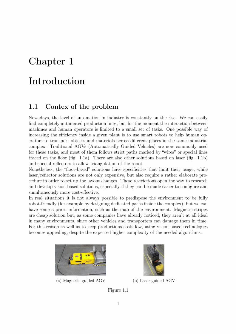
1.1 Contex of the problemNowadays, the level of automation in industry is constantly on the rise. We can easilyfind completely automated production lines, but for the moment the interaction betweenmachines and human operators is limited to a small set of tasks. One possible way ofincreasing the efficiency inside a given plant is to use smart robots to help human op-erators to transport objects and materials across different places in the same industrialcomplex. Traditional AGVs (Automatically Guided Vehicles) are now commonly usedfor these tasks, and most of them follows strict paths marked by “wires” or special linestraced on the floor (fig. 1.1a). There are also other solutions based on laser (fig. 1.1b)and special reflectors to allow triangulation of the robot.Nonetheless, the “floor-based” solutions have specificities that limit their usage, whilelaser/reflector solutions are not only expensive, but also require a rather elaborate pro-cedure in order to set up the layout changes. These restrictions open the way to researchand develop vision based solutions, especially if they can be made easier to configure andsimultaneously more cost-effective.In real situations it is not always possible to predispose the environment to be fullyrobot-friendly (for example by designing dedicated paths inside the complex), but we canhave some a priori information, such as the map of the environment. Magnetic stripesare cheap solution but, as some companies have already noticed, they aren’t at all idealin many environments, since other vehicles and transporters can damage them in time.For this reason as well as to keep productions costs low, using vision based technologiesbecomes appealing, despite the expected higher complexity of the needed algorithms.

(a) Magnetic guided AGV (b) Laser guided AGV

Figure 1.1

1

1.2 State of the artNowadays, it is very common to find AGVs in many industry fields. It is interesting tonotice that many types of technologies can be used to allow the self-localization of thesespecials robots, each one with its own advantages and disadvantages.As it will be shown in subsection 1.2, using different approaches means using differentkinds of sensors. The problem of how to efficiently combine all the information providedby a number of different (and in general heterogeneous) sensors is widely discussed in theliterature of the last years and it is usually referred as the problem of sensor fusion. Acommon solution to this problem is using the Kalman Filter [1] or one of its declinations(for instance the Extended Kalman Filter [2] or the Unscented Kalman Filter [3]).

In the particular case of this thesis, the robot used to test the algorithms (AtlasMV[4]) is a car-like robot, and this makes the problem of the sensor fusion not much dif-ferent from the problem of outdoor localization of a common car with a GPS (GlobalPositioning System)[5]; instead of the estimation of the position provided by a GPS, theestimation of the position provided by visual information can be used.Also, the estimation of the position obtained through vision algorithms and special mark-ers can be obtained using trilateration and/or triangulation algorithms. Many authorsare working on this topic and the same problem can be solved using a variety of differentapproaches. [6] has presented a method based on an Extended Kalman Filter with astate-vector composed of the external angular measurements. [7] has presented a simple,fast and new three object triangulation algorithm based on the power center of three cir-cles. [8] has presented an algorithm for automatic selection of optimal landmarks whichcan reduce the uncertainty by more than one order of magnitude.

This thesis must be considered as the continuation of a previous thesis work accom-plished by Luís Carrão[9], where the library Libdmtx and the triangulation/trilaterationalgorithm have been tested. Also, an extended analysis of the localization accuracy hasbeen accomplished.

2

Most common systems

This subsection gives a brief overview of which kind of systems are available on themarket. One of the most innovative systems available on the industry is the Kiva Sys-tem[10][11]: this system can coordinate hundreds of mobile robots in the same warehouseand the robot’s navigation system involves a combination of dead reckoning and cam-eras that look for fiducial markers, that are placed on the floor during system installation.

The most commonly used systems are:

• magnetic stripe system;

• optical guided system;

• inertial navigation system;

• laser guide system;

• vision system.

Further information is provided in the following subsections.

Magnetic stripe system

The magnetic stripe system works thanks to electric current passing through a guide wireinstalled along the travel route on or in the floor; the AGV travels along the magneticfield produced by the current. This system is simple but any change on the route requiresto remove the old magnetic stripe and to install a new one. Moreover, especially if thestripe is on the floor, constant maintenance is needed, since the stripe tends to deterioratein time because of mechanical stress, and any breakage of the wires makes it impossibleto detect the route.

Optical guided system

With the optical guided system, reflective tape made of aluminium or a similar materialis laid along the travel route, and the AGV determines its route by optically detectingthe tape. A common problem of this system is the difficulty to detect the tape when itis dirty or damaged.

Inertial navigation system

An inertial sensor (gyro and accelerometer) mounted on the AGV is used to measurethe vehicle’s attitude angle and travel distance. The current position is calculated usingmeasurement data, and the AGV travels along the set route. Transponders embeddedin the floor are used to verify that the vehicle is following the correct path. This systemrequires the installation of corrective markers along the paths because the error of inertialsystems tend to accumulate as an integral term.

3

Laser guide system

A laser beam from the AGV is reflected by reflectors mounted on walls and the currentposition is determined by the angle (and sometimes the distance) of the reflected light,and the vehicle uses this data to travel along the set route. The collected information iscompared to the map of the reflector layout stored in the AGV’s memory and using atriangulation (or trilateration) algorithm the robot can calculate its position and followits route.

Vision guide system

Vision-guided AGVs work using cameras to record features along the route. A robot thatuses this system requires a map, in which the features have been previously recorded. It ispossible to use different combination of cameras, for instance stereo and omnidirectional.The extraction of the features from an image requires a higher computational power incomparison to the one needed for the other systems, but this system has the advantageof not requiring any kind of landmarks, tape, wire or stripe.

4

1.3 Proposed solution

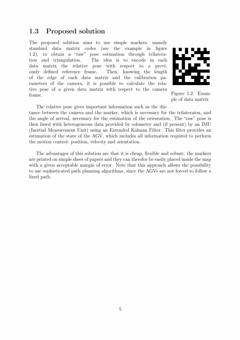
Figure 1.2: Exam-ple of data matrix

The proposed solution aims to use simple markers, namelystandard data matrix codes (see the example in figure1.2), to obtain a “raw” pose estimation through trilatera-tion and triangulation. The idea is to encode in eachdata matrix the relative pose with respect to a previ-ously defined reference frame. Then, knowing the lengthof the edge of each data matrix and the calibration pa-rameters of the camera, it is possible to calculate the rela-tive pose of a given data matrix with respect to the cameraframe.

The relative pose gives important information such as the dis-tance between the camera and the marker, which is necessary for the trilateraion, andthe angle of arrival, necessary for the estimation of the orientation. The “raw” pose isthen fused with heterogeneous data provided by odometry and (if present) by an IMU(Inertial Measurement Unit) using an Extended Kalman Filter. This filter provides anestimation of the state of the AGV, which includes all information required to performthe motion control: position, velocity and orientation.

The advantages of this solution are that it is cheap, flexible and robust: the markersare printed on simple sheet of papers and they can therefor be easily placed inside the mapwith a given acceptable margin of error. Note that this approach allows the possibilityto use sophisticated path planning algorithms, since the AGVs are not forced to follow afixed path.

5

6

Chapter 2

Overview

2.1 Development platform

During this work many tools have been used. This section presents a brief introductionof the platform used, more details will be added in the following chapters.

2.1.1 ROS - Robot Operating System

ROS[12] is an open source framework used to build advanced robot applications. It wasoriginally developed in 2007 by the SAIL (Sanford Artificial Intelligence Laboratory) andthrough the years it has become a de facto standard in the research field. Its appeal isgrowing even in the industry, thanks to the ROS-Industrial consortium. ROS is designedto be flexible, general-purpose and robust. It includes a constantly increasing number oftools, libraries and interfaces that can be reused and improved by anyone.One of the key features of this framework is the possibility to use virtually any pro-gramming language. At this moment the main supported languages are C++, Java andPython. A ROS program is typically subdivided in two or more “nodes”: which are is infact a stand alone programs, able both to provide functionalities and to use functionalitiesprovided by others nodes. The communication between nodes is made possible thanksto a standard common interface based on “messages”. The interface is implemented overthe TPC/IP protocol: this means that each message sent by a node is converted in aseries of TCP/IP packet received by other nodes, even if they run in different machinesconnected to the same network.

2.1.2 Robotics System Toolbox

The new Robotics System Toolbox (RST)[13] has been introduced in MATLAB R2015a.This new toolbox successfully uses the Java implementation of ROS, presented by Googlein 2011, in order to provide an interface between MATLAB-Simulink and ROS. Thistoolbox allows the rapid prototyping of algorithms and their integration directly in theROS workspace, opening the possibility of using MATLAB and Simulink algorithms withreal (or simulated) ROS-compliant robots with minimal code changes.The following chapters will show how MATLAB and RST were widely used in order to

7

perform simulations, to test algorithms before writing them in C++ and to analyse thecollected data.

2.1.3 Libdmtx library

Libdmtx[14] is an open source software for encoding and decoding Data Matrix. Thislibrary is written in C, has a rather good performance level and a stability sufficient forthe purpose of this thesis. This library is also used by many ROS packages, fox examplecob-marker and visp-auto-tracker.

2.1.4 OpenCV library

OpenCV (Open Source Computer Vision)[15] is a cross-platform library mainly aimed atreal-time computer vision. The library is written in C (version 1.x) and C++ (version 2.xand 3.x) and there are full interfaces in Python, Java, MATLAB and others languages.It is also the primary vision package in ROS. As explained in the next pages, in thisthesis it has been used to handle the following operations:

• all geometrical transformations between different reference frames;

• the camera calibration;

• the calculation of the relative pose between data matrix and camera.

In addition to these features, a basic interface to usb cameras is provided.

2.1.5 Qt framework

Qt ("cute")[16] is a cross-platform application framework used mainly for developingapplication software with graphical user interfaces (GUI). It is perfectly integrated inROS and it has been used to develop a utility which allows to:

• easily import maps (in a bitmap format);

• collocate and automatically generate data matrices containing their poses relativeto a fixed reference frame;

• save and open projects;

• print or export each data matrix in .png or .pdf.

This application will be presented in the next chapter.

Figure 2.1: From left to right: OpenCV, ROS, Qt, Libdmtx, MATLAB logos.

8

2.2 Validation hardware platformA real robot equipped with two cameras, one looking forward and one looking backward,has been used in order to validate the developed algorithms and to collect data. Thecollected information has been fundamental to understand which were the main sourcesof uncertainty and problems.

2.2.1 AtlasMV robot

The robot, named AtlasMV[4] (fig. 2.2a), has been developed by the University of Aveiroin 2008 to participate in robotics competitions. AtlasMV is a car-like robot with a fullyfunctioning ROS interface. Through this interface, it is possible to control both speedand steering angle and to read their relative estimations at a frequency of 30Hz. Also, itis possible to get further information regarding the status of the robot.

2.2.2 Video capturing devices

Two Logitech R© c310 cameras (fig. 2.2b) have been used for capturing visual information.These cameras are capable of capturing images with a frequency up to 30hz (dependingon the exposure time) and at a resolution up to 1280x960 pixel. These cameras are notoriented to computer vision, with a good tuning it was nevertheless possible to obtainimages with a sufficient quality even in non static situations.

(a) AtlasMV equipped with two cameras(red cirle) (b) Logitech R© c310 usb camera

Figure 2.2

9

10

Chapter 3

Map characterization, informationencoding and tools creation

3.1 Map characterization

The first problem that has been considered was how to properly prepare a given environ-ment to allow the localization of a robot using visual information.As a starting point it has been assumed that the map of the environment is known andavailable as a bitmap image. Then, the following step has been to take an arbitrary frameof the map as origin of the 2D Cartesian coordinate system, defined as map frame andindicated with Omap. In analogy to the coordinate system often used in computer visionlibraries (like OpenCV) the top-left corner of the image has been fixed as origin of thecoordinate system, with X axis pointing right and the Y axis pointing up.The figure 3.1 shows a partial map of LAR1, where most of the tests with the AtlasMVhave been executed. The fig.3.1 shows the map frame at the top-left corner of the image(the border of the image represented with a blue line).

Figure 3.1: The map of LAR

1Laboratory for Automation and Robotics - Department of Mechanical Engineering at the Universityof Aveiro.

11

3.2 Information encodingThe second problem that has been considered was that of finding the best trade-off be-tween the amount of information encoded in a data matrix and the dimension of thesymbol. This problem is related to the fact that the robot must be able to detect anddecode a given data matrix from a distance of at least 4/5 meters, otherwise the local-ization system would be useless.

According to the last standard ECC 200[17][18], the symbol size can vary from 9x9to 144x144; the table 3.1 resumes some interesting properties of the data matrices (notall the format numbers are reported for brevity).

It is reasonable to approximate the 2D coordinate system previously defined with agrid-based representation obtained by embedding the map into a discretized coordinatesystem with a step of 0.1m (one order of magnitude smaller than the typical dimensionsof an AGV).

As reported in the table 3.1, the minimum symbol size is 10x10 (format number 0 )and in it 1 byte of information can be stored. A symbol with this size and printed on aA4 sheet of paper can be easily decoded2, but 1 byte is not sufficient most in practicalcases: if the byte is equally divided (4 bits for the X axis and 4 for the Y axis) then it ispossible to represent only a map with a size of 1.6m x 1.6m.

The second option that was taken into consideration is the format number 1. With asymbol size of 12x12, the format number 1 can store 3 bytes of data. Dividing the bytesequally (12 bits for the X axis and 12 for the Y axis) it is possible to represent a mapwith a size of 409.6m x 409.6m, that is more than enough for most applications.

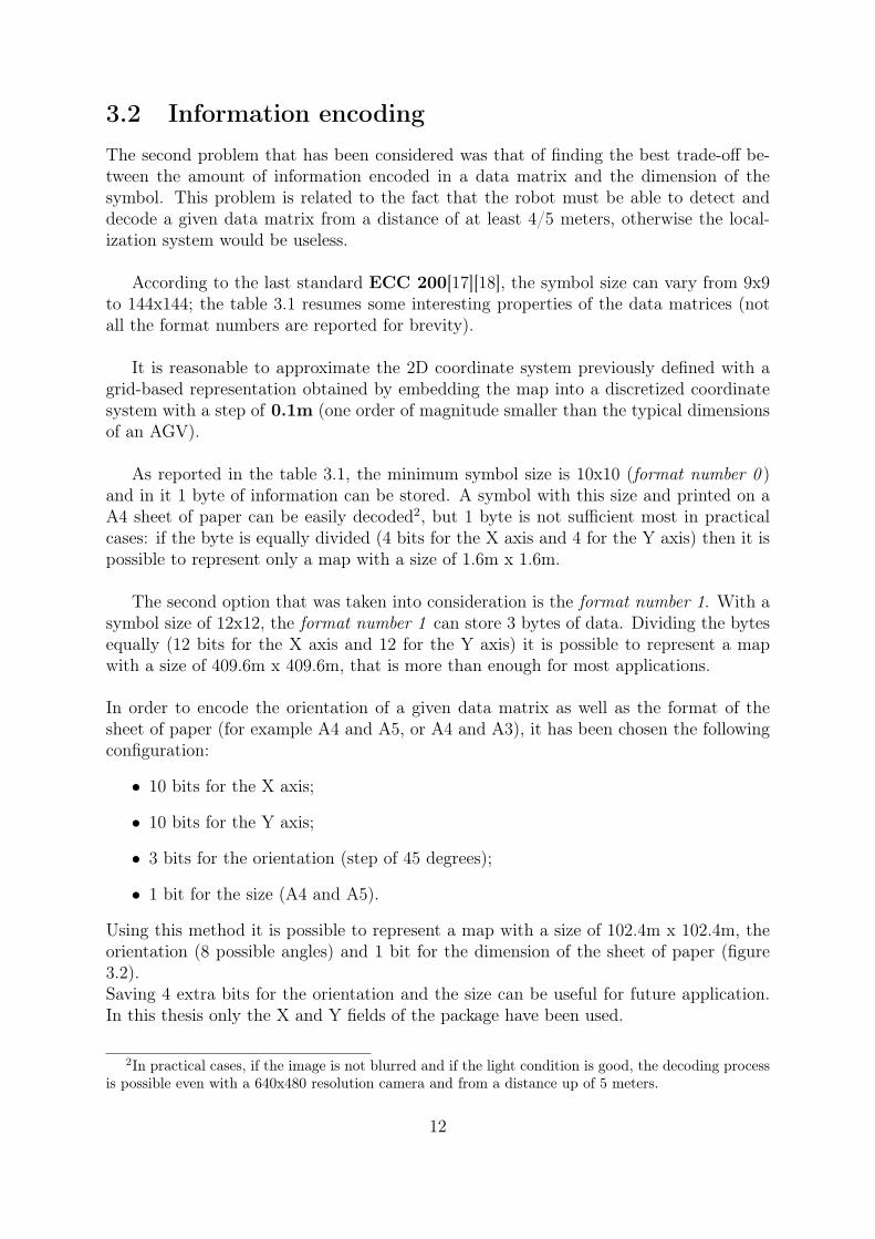
In order to encode the orientation of a given data matrix as well as the format of thesheet of paper (for example A4 and A5, or A4 and A3), it has been chosen the followingconfiguration:

• 10 bits for the X axis;

• 10 bits for the Y axis;

• 3 bits for the orientation (step of 45 degrees);

• 1 bit for the size (A4 and A5).

Using this method it is possible to represent a map with a size of 102.4m x 102.4m, theorientation (8 possible angles) and 1 bit for the dimension of the sheet of paper (figure3.2).Saving 4 extra bits for the orientation and the size can be useful for future application.In this thesis only the X and Y fields of the package have been used.

2In practical cases, if the image is not blurred and if the light condition is good, the decoding processis possible even with a 640x480 resolution camera and from a distance up of 5 meters.

12

bit

Y

xOrientation

A4A5

10bits 10bits 3bits 1

Figure 3.2: Data package encoded

It is important to notice that with the chosen coordinate system, the X value is alwayspositive, and the Y value is always negative. In order to save data, it has been chosento encode only the absolute value of Y. The minus sign is later reintroduced during thedecoding process.

Table 3.1: Data Matrix Formats

Format number Size Max binary capacity % of codewords forerror correction

correctablecodewords

0 10x10 1 62.5 2-01 12x12 3 58.3 3-02 14x14 6 55.6 5-73 16x16 10 50 6-9... ... ... ... ...20 104x104 814 29.2 168-31821 120x120 1048 28 204-39022 132x132 1302 27.6 248-47223 144x144 1556 28.5 310-590

Each codeword is represented in the data matrix by a square part of 8 modules,corresponding to 8 bits. Depending on the symbol size, there is a portion of codewordsused to correct errors. The error-correction codes used are the Reed-Solomon codes[19].For instance, the format number 2 has 58.3% of codewords dedicated to error correctionand up 3 codewords can be corrected.

13

3.3 Application: "Datamatrix generator"

In order to provide a simple tool for generating special data matrices, it has been devel-oped an application using the Qt framework. As anticipated in the sub section 2.1.5, thisapplication covers all the processes of landmarks creation and is specifically dedicated tothe generation of datamatrix for indoor labeling and localization.

The figure 3.3 shows how the application looks like on its first run. Six areas havebeen highlighted:

1. Open or save projects (a project contains the map, the scale and the list of datamatrices);

2. zoom in and out the map view;

3. add a new marker with a given position and a given orientation;

4. load a map from an image (png, jpg and other formats are supported);

5. print an item (the marker is converted to a data matrix during the printing process);

6. display all the data matrices added to the map in a dedicated table.

1

2 3 45

6

Figure 3.3: Data matrix application

14

By pressing the Load Map button, it is possible to select an image containing a map.The following step is to enter the correct scale factor (figure 3.4).

Figure 3.4: Set the scale factor.

The figure 3.5 shows how the creation and the positioning of a given data matrixworks: each data matrix can be moved by using the drag and drop functionality or usingthe Edit item window, which opens with a double-click on the item. Using the Edit itemwindow it is also possible to change the orientation or to delete a given item.

Figure 3.5: Add a new item.

15

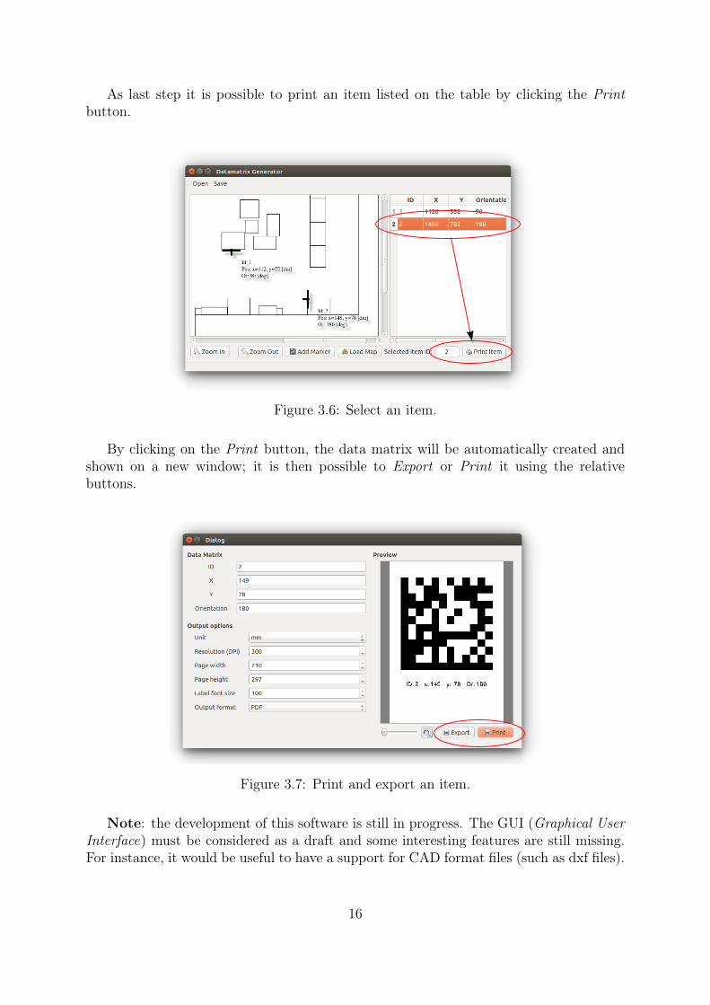
As last step it is possible to print an item listed on the table by clicking the Printbutton.

Figure 3.6: Select an item.

By clicking on the Print button, the data matrix will be automatically created andshown on a new window; it is then possible to Export or Print it using the relativebuttons.

Figure 3.7: Print and export an item.

Note: the development of this software is still in progress. The GUI (Graphical UserInterface) must be considered as a draft and some interesting features are still missing.For instance, it would be useful to have a support for CAD format files (such as dxf files).

16

Chapter 4

Perception

This chapter covers the topics relative to perception: from camera calibration to thecalculation of the relative pose of a camera according to a data matrix.

4.1 Pinhole camera

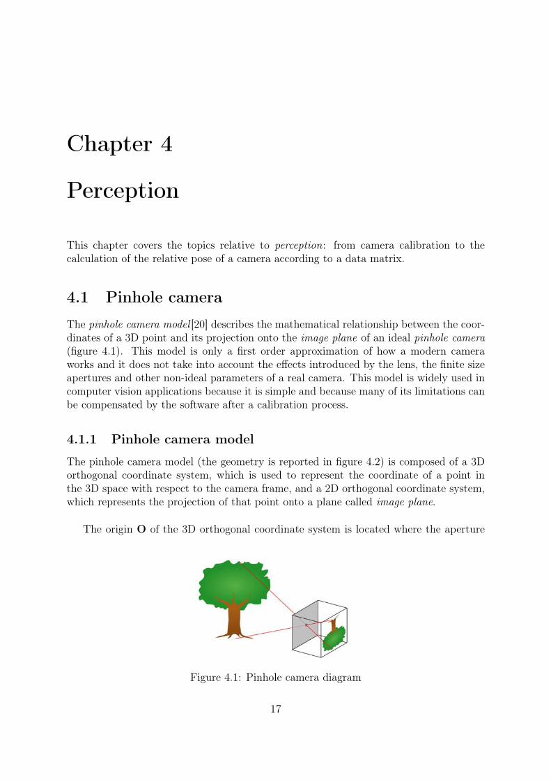
The pinhole camera model [20] describes the mathematical relationship between the coor-dinates of a 3D point and its projection onto the image plane of an ideal pinhole camera(figure 4.1). This model is only a first order approximation of how a modern cameraworks and it does not take into account the effects introduced by the lens, the finite sizeapertures and other non-ideal parameters of a real camera. This model is widely used incomputer vision applications because it is simple and because many of its limitations canbe compensated by the software after a calibration process.

4.1.1 Pinhole camera model

The pinhole camera model (the geometry is reported in figure 4.2) is composed of a 3Dorthogonal coordinate system, which is used to represent the coordinate of a point inthe 3D space with respect to the camera frame, and a 2D orthogonal coordinate system,which represents the projection of that point onto a plane called image plane.

The origin O of the 3D orthogonal coordinate system is located where the aperture

Figure 4.1: Pinhole camera diagram

17

is located (or in the geometric center of the aperture in case of a real camera with finitesize aperture), the X3 axis is pointing in the viewing direction of the camera and it refersto its optical axis (or principal axis). The X1 and X2 axes locate the principal plane.

The image plane is parallel to the axes X1 and X2 and it is located at a distance ffrom the origin O in the negative direction of the X3 axis. The value f is referred toas the focal length. The point R is placed at the intersection of the optical axis and theimage plane and it is called principal point (or image center).

A given point P at coordinate (x1,x2,x3) relative to the axes X1,X2,X3 projectedonto the image plane is defined as Q. The coordinate of the point Q relative to the 2Dcoordinate system are expressed as (y1,y2).

Image plane

f

Y1

Y2

QR

O

X2

X1

X3

P

x1

x2

x3

Figure 4.2: Pinhole model

18

The relation between the 3D coordinates (x1,x2,x3) of point P and its image coordi-nates (y1,y2) given by point Q in the image plane is expressed by(

y1

y2

)= − f

x3

(x1

x2

). (4.1)

Note that the image in the image plane is rotate by π. In order to produce an unrotatedimage, it is useful to define a virtual plane so that it intersects the X3 axis at f insteadof −f . The resulting mapping from 3D to 2D coordinates is given by(

y1

y2

)=

f

x3

(x1

x2

). (4.2)

The relation 4.2 can’t provide the 3D coordinate of a point from its 2D projection butonly the ratios x1

x3and x2

x3(fig.4.3): which means that with a single camera it is impossible

to determine the 3D coordinate of a point.

Figure 4.3: Relation between y1f

and x1x3

In the general case, in order to determine the position of a given point it is necessaryto use a stereo vision system and the epipolar geometry [21]. In the particular case thathas been considered, it has not been necessary to use more than one camera: knowing thegeometry of a data matrix, which is approximable to a square with a given edge length,it is possible to calculate its pose with only one camera if at least three correspondencesbetween image points and objects points have been identified[22].

19

4.1.2 Camera calibration

The calibration process allows the identification of the intrinsic parameters and distortioncoefficients of the camera. Without this step it is impossible to obtain a good accuracy,especially when the lens introduce a high distortion.The intrinsic parameters are necessary for defining the camera matrix, that is

K := KsKf =

sx sθ Ox

0 sy Oy

0 0 1

f 0 00 f 00 0 1

=

fsx fsθ Ox

0 fsy Oy

0 0 1

, (4.3)

where

• sx and sy are scale factors;

• sθ is the skew factor;

• Ox and Oy are the offsets of the central point;

• f is the focal length.

Using the homogeneous coordinates, the camera matrix defines the relation

λ

y1

y2

1

= K

x1

x2

x3

, λ 6= 0 . (4.4)

The distortion coefficients are used to compensate the radial and tangential distortionintroduced by lens. Figure 4.4 shows distorted chessboard (figure 4.4a) during the cali-bration procedure and the undistorted chessboard after the calibration (figure 4.4b). Thesoftware used for the calibration is the ROS package camera-calibration[23].

(a) A chessboard during the calibration (b) A chessboard after the calibration

Figure 4.4: Camera calibration process

20

4.2 Data Matrix pose with respect to the camera frame

In the previous chapter the pinhole model and the concept of camera calibration werediscussed. This section presents the approach used for obtaining the pose of a given DataMatrix with respect to the camera frame, defined as Ocam.

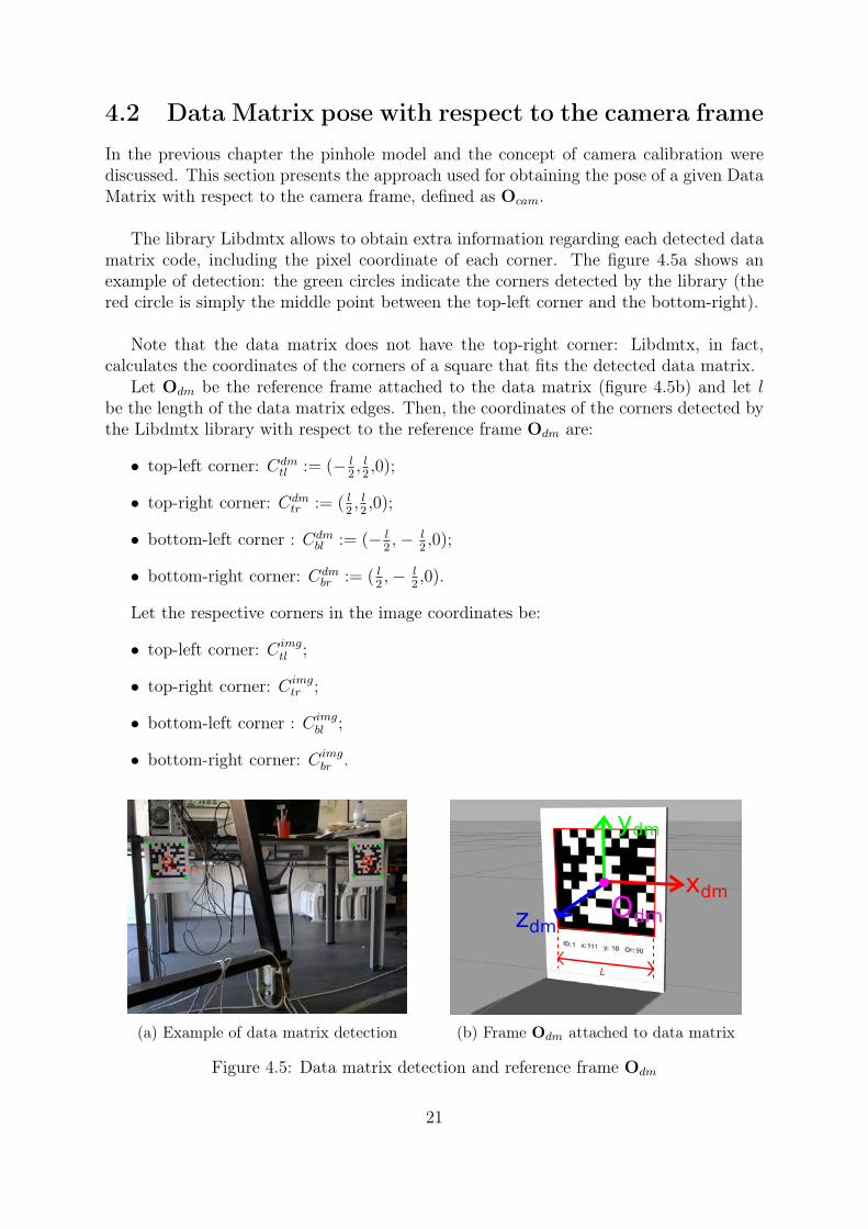
The library Libdmtx allows to obtain extra information regarding each detected datamatrix code, including the pixel coordinate of each corner. The figure 4.5a shows anexample of detection: the green circles indicate the corners detected by the library (thered circle is simply the middle point between the top-left corner and the bottom-right).

Note that the data matrix does not have the top-right corner: Libdmtx, in fact,calculates the coordinates of the corners of a square that fits the detected data matrix.

Let Odm be the reference frame attached to the data matrix (figure 4.5b) and let lbe the length of the data matrix edges. Then, the coordinates of the corners detected bythe Libdmtx library with respect to the reference frame Odm are:

• top-left corner: Cdmtl := (− l

2, l2,0);

• top-right corner: Cdmtr := ( l

2, l2,0);

• bottom-left corner : Cdmbl := (− l

2,− l

2,0);

• bottom-right corner: Cdmbr := ( l

2,− l

2,0).

Let the respective corners in the image coordinates be:

• top-left corner: Cimgtl ;

• top-right corner: Cimgtr ;

• bottom-left corner : Cimgbl ;

• bottom-right corner: Cimgbr .

(a) Example of data matrix detection

L

xdm

ydm

zdmOdm

(b) Frame Odm attached to data matrix

Figure 4.5: Data matrix detection and reference frame Odm

21

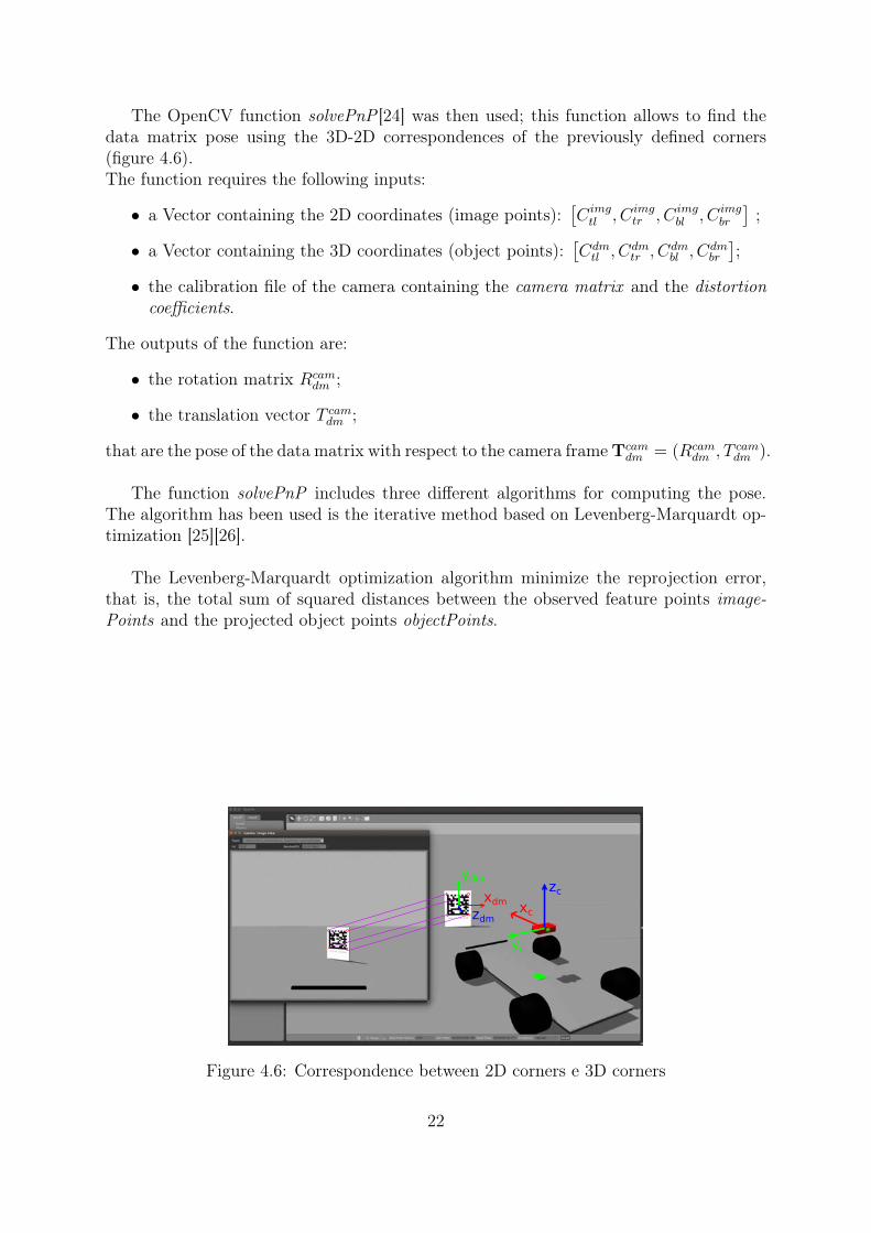
The OpenCV function solvePnP [24] was then used; this function allows to find thedata matrix pose using the 3D-2D correspondences of the previously defined corners(figure 4.6).The function requires the following inputs:

• a Vector containing the 2D coordinates (image points):[Cimgtl , Cimg

tr , Cimgbl , Cimg

br

];

• a Vector containing the 3D coordinates (object points):[Cdmtl , C

dmtr , C

dmbl , C

dmbr

];

• the calibration file of the camera containing the camera matrix and the distortioncoefficients.

The outputs of the function are:

• the rotation matrix Rcamdm ;

• the translation vector T camdm ;

that are the pose of the data matrix with respect to the camera frameTcamdm = (Rcam

dm , T camdm ).

The function solvePnP includes three different algorithms for computing the pose.The algorithm has been used is the iterative method based on Levenberg-Marquardt op-timization [25][26].

The Levenberg-Marquardt optimization algorithm minimize the reprojection error,that is, the total sum of squared distances between the observed feature points image-Points and the projected object points objectPoints.

zc

xc

yc

xdm

ydm

zdm

Figure 4.6: Correspondence between 2D corners e 3D corners

22

4.3 Data matrix pose with respect to the robot frameOne of the aims of the localization algorithm was to use two or more cameras to scan awider area around the robot. In order to simplify the localization algorithm, it has beennecessary to calculate the pose of each data matrix with respect to a given reference frame.

The adopted approach makes the whole algorithm modular : the part of the algorithmthat estimates the position doesn’t have to be aware of how many cameras the robotemploys but only it needs to know the pose of each data matrix in relation to that givenreference frame.

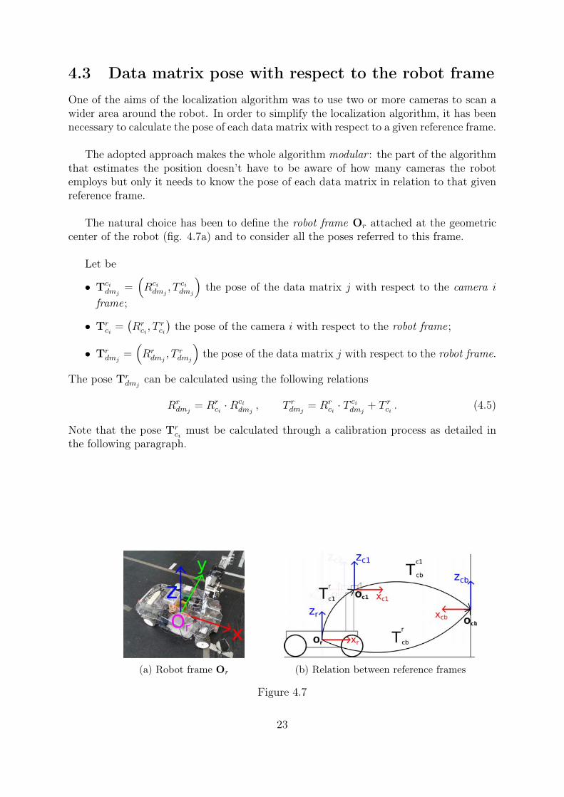
The natural choice has been to define the robot frame Or attached at the geometriccenter of the robot (fig. 4.7a) and to consider all the poses referred to this frame.

Let be

• Tcidmj

=(Rcidmj

, T cidmj

)the pose of the data matrix j with respect to the camera i

frame;

• Trci

=(Rrci, T rci

)the pose of the camera i with respect to the robot frame;

• Trdmj

=(Rrdmj

, T rdmj

)the pose of the data matrix j with respect to the robot frame.

The pose Trdmj

can be calculated using the following relations

Rrdmj

= Rrci·Rci

dmj, T rdmj

= Rrci· T cidmj

+ T rci . (4.5)

Note that the pose Trci

must be calculated through a calibration process as detailed inthe following paragraph.

x

y

z

(a) Robot frame Or (b) Relation between reference frames

Figure 4.7

23

Extrinsic camera parameters

The calculation of the pose Trcihas required to develop a specific calibration process since

only the pose of Tcidmj

is computed and the direct calculation of the pose Trci(especially

the orientation) is not easy in practice.

The calibration process uses a chessboard situated in a known position with respect tothe robot frameOr. The pose of the chessboard with respect to the camera i frame Tci

cb :=(Rci

cb, Tcicb ) has been calculated using the built-in OpenCV function findChessboardCorners

(in order to get the corners coordinates) and then again the function solvePnP.The relations that were used are the following:

Rrci

= Rrcb · (R

cicb)−1 , (4.6)

T rci = T rcb −Rrci· T cicb = T rcb −Rr

cb · (Rcicb)−1 · T cicb . (4.7)

LetOc1 be the coordinate system of the camera that looks forward andOc2 the coordinatesystem of the camera that looks backward. The figure 4.7b shows the relation betweenthe reference frames Or, Oc1 and Ocb.In the example shown in figure 4.8, the chessboard has been positioned in a specific pointsuch that the resulting pose Tr

cb (measured with a measuring tape) was

T rcb =

1.540

0.75

[meters] , Rrcb =

cos π − sinπ 0sinπ cosπ 0

0 0 1

. (4.8)

The calibration has been executed using a C++ program developed for this task and thepose Tr

cihas been calculated using the relations 4.6 and 4.7 and the OpenCV function

composeRT [24].

Figure 4.8: Extrinsic parameters calibration

24

4.4 Implementation of the algorithmThe algorithm described in this chapter has been implemented as a single ROS nodecalled datamatrix-pose-pub. This node includes the following components:

• an interface to the cameras, using OpenCV’s APIs;

• a data matrix detector, using Libdmtx;

• the computation of Tcidmj

, for each camera i and each data matrix j, using solvePnP ;

• the computation of Trdmj

, using composeRT.

The figure 4.9 is a schematic of the internal architecture of this node.

Figure 4.9: Structure of the node datamatrix-pose-pub

The frames are captured using the same target, timestamped for both cameras. Thishas been necessary for two reasons:

• to keep track of the acquisition timestamp (this information is important becausethe delay introduced by the datamatrix detection process must be taken into ac-count);

• to avoid errors introduced when the localization algorithm attempts to estimatethe position of the robot using a couple of data matrices detected in two differentframes with different timestamps.

The frame is elaborated by the Libdmtx library and the pose of each detected datamatrix is calculated using the proper calibration file and the OpenCV function solvePnP.

25

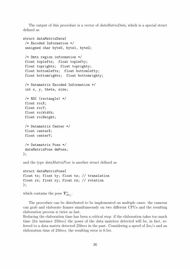
The output of this procedure is a vector of dataMatrixData, which is a special structdefined as

struct dataMatrixData{/* Encoded Information */unsigned char byte0, byte1, byte2;

/* Dmtx region information */float topleftx; float toplefty;float toprightx; float toprighty;float bottomleftx; float bottomlefty;float bottomrightx; float bottomrighty;

/* Datamatrix Encoded Information */int x, y, theta, size;

/* ROI (rectangle) */float roiX;float roiY;float roiWidth;float roiHeight;

/* Datamatrix Center */float centerX;float centerY;

/* Datamatrix Pose */dataMatrixPose dmPose;

};

and the type dataMatrixPose is another struct defined as

struct dataMatrixPose{float tx; float ty; float tz; // translationfloat rx; float ry; float rz; // rotation};

which contains the pose Tcidmj

.

The procedure can be distributed to be implemented on multiple cases: the camerascan grab and elaborate frames simultaneously on two different CPUs and the resultingelaboration process is twice as fast.Reducing the elaboration time has been a critical step: if the elaboration takes too muchtime (for instance 250ms) the poses of the data matrices detected will be, in fact, re-ferred to a data matrix detected 250ms in the past. Considering a speed of 2m/s and anelaboration time of 250ms, the resulting error is 0.5m.

26

The vectors relative to each elaboration thread are finally processed sequentially usingthe function composeRT and the extrinsic parameters of each camera. The resultingoutput is a data structure called DataMatrixPoseSet, which is a custom ROS messagewith the following structure

Header headerfloat64 acq_timestampdatamatrix_detection/DatamatrixPose[] dmpose

where header is a ROS data type used for managing the messages, acq-timestamp is theacquisition timestamp and dmpose is a vector of DatamatrixPose, which is a custom ROSmessage defined as

float64 dm_msg_xfloat64 dm_msg_yfloat64 dm_msg_orfloat64 dm_msg_sizegeometry_msgs/PoseWithCovariance pose

The message DatamatrixPoseSet is finally published on the ROS topic datamatrix-pose at a frequency between 10Hz and 15Hz. This frequency has been determined bythe computational power of CPU used, an Intel R© CoreTM i3-2310m (dual-core processorwith a frequency up to 2,1GHz).

The messages published on this topic are read by the ROS node named atlasmv-ekf,which is presented in the chapter 5.

27

28

Chapter 5

Estimation of position and sensorfusion

This chapter covers the part of the thesis regarding position estimation and sensor fusionof the moving robot.The covered topics are:

• localization using trilateration and triangulation techniques;

• AtlasMV modelling using a bicycle-like model;

• sensor fusion using an Extended Kalman Filter;

• model verification using Simulink.

5.1 Localization using trilateration and triangulationIn the context of this problem, the robot should be able to estimate its own position inthe environment every time at least two data matrices are detected by its own camerasystem.Let be:

• raw-robot-pose, the pose of the robot obtained using only the visual information ata given time t;

• ekf-robot-pose, the filtered pose of the robot obtained using the Extended KalmanFilter.

This section presents how raw-robot-pose is calculated.As seen in the previous chapter, the datamatrix-pose-pub node provides a vector con-

taining the poses of the j − th data matrix with respect to the robot frame, Trdmj

: theposes are referred to the 3D coordinate frame of the robot, Or. On the contrary, theestimated position is referred to the coordinate system of the map, Omap.

Assuming that the robot is moving on a plane domain and hence the axes xr and yrof the robot frame Or are parallel to the axes xmap and ymap of the map frame Omap, it is

29

possible to simply ignore the zr axis and to keep on working on a 2D coordinate system.In this context, the robot pose with respect to the map frame Omap can be determinedusing the coordinates (x, y, θ)(fig. 5.1), where x and y are the coordinates with respect tothe axes xmap and ymap, and θ is the orientation (rotation angle with respect to the z axis).

Let dmj be the j − th detected data matrix. The localization algorithm uses thefollowing information extracted from the dataMatrixData structure:

• xencj and yencj , the encoded pose of the data matrix with respect to the map frame;

• Tr,2Ddmj

:= (xj, yj), 2D translation vector extracted from Trdmj

= (xj, yj, zj);

To keep the notation light, the vector Trdmj

will indicate both Trdmj

and Tr,2Ddmj

.

If dm1 and dm2 are two detected data matrices, it is possible to define the distanceand the angle with respect to the robot frame using the relations:

dj :=√x2j + y2

j , αj = arctan 3

(yjxj

), j = 1, 2 (5.1)

where arctan 3 (·) is an arctan (·) function defined in [0, 2π].

Let C1 and C2 be the circumferences with center in (xenc1 , yenc1 ) and (xenc2 , yenc2 ), and withradius d1 and d2, respectively. The robot position (x, y) is in one of the intersection pointsP1 and P2 (fig. 5.2) of the circumferences (the cases with one or zero intersections aresimply ignored by the algorithm).

It is easy to ascertain which position is the correct one, namely through a simple com-parison between the measured angles αj and the angles obtained using the coordinatespoints P1 and P2 and the coordinates xencj and yencj , with j = 1,2.

Figure 5.1: Robot pose (x, y, θ).

30

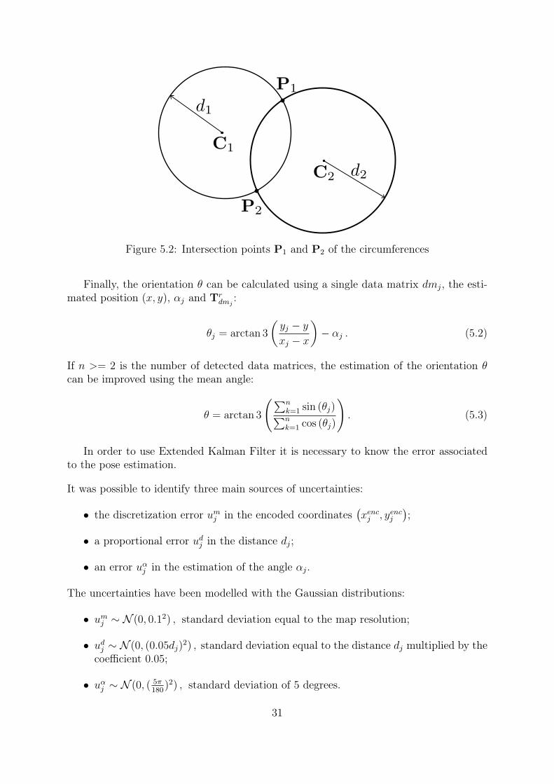
Figure 5.2: Intersection points P1 and P2 of the circumferences

Finally, the orientation θ can be calculated using a single data matrix dmj, the esti-mated position (x, y), αj and Tr

dmj:

θj = arctan 3

(yj − yxj − x

)− αj . (5.2)

If n >= 2 is the number of detected data matrices, the estimation of the orientation θcan be improved using the mean angle:

θ = arctan 3

(∑nk=1 sin (θj)∑nk=1 cos (θj)

). (5.3)

In order to use Extended Kalman Filter it is necessary to know the error associatedto the pose estimation.

It was possible to identify three main sources of uncertainties:

• the discretization error umj in the encoded coordinates(xencj , yencj

);

• a proportional error udj in the distance dj;

• an error uαj in the estimation of the angle αj.

The uncertainties have been modelled with the Gaussian distributions:

• umj ∼ N (0, 0.12) , standard deviation equal to the map resolution;

• udj ∼ N (0, (0.05dj)2) , standard deviation equal to the distance dj multiplied by the

coefficient 0.05;

• uαj ∼ N (0, ( 5π180

)2) , standard deviation of 5 degrees.

31

It has been assumed by hypothesis that the uncertainties are uncorrelated.

Let xyθ

= p

xencj

yencj

djαj

, j = 1, ..., n

(5.4)

be the function that calculates the estimation of the pose.The resulting error has been calculated numerically using the first order propagation ofuncertainty formula:

u

xyθ

=n∑j=1

√(∂p

∂xj

)2

(umj )2 +

(∂p

∂yj

)2

(umj )2 +

(∂p

∂dj

)2

(udj )2 +

(∂p

∂αj

)2

(uαj )2

, j = 1, ..., n. (5.5)

Let

e =

exeyeθ

:= u

xyθ

(5.6)

be the error vector associated to the estimation of the pose. The measurement obtainedat the time t can be written as

yv(t) =

x(t)y(t)θ(t)

, cov(yv(t) · yTv (t)

):=

ex(t) 0 00 ey(t) 00 0 eθ(t)

, (5.7)

where the subscript v stands for vision.

32

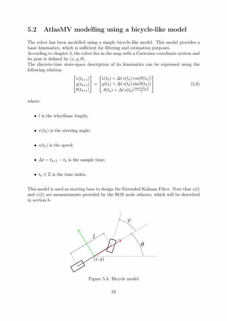
5.2 AtlasMV modelling using a bicycle-like model

The robot has been modelled using a simple bicycle-like model. This model provides abasic kinematics, which is sufficient for filtering and estimation purposes.According to chapter 3, the robot lies in the map with a Cartesian coordinate system andits pose is defined by (x, y, θ).The discrete-time state-space description of its kinematics can be expressed using thefollowing relation: x(tk+1)

y(tk+1)θ(tk+1)

=

x(tk) + ∆t s(tk) cos(θ(tk))y(tk) + ∆t s(tk) sin(θ(tk))

θ(tk) + ∆t s(tk)tan(ψ(tk))

l

(5.8)

where:

• l is the wheelbase length;

• ψ(tk) is the steering angle;

• s(tk) is the speed;

• ∆t = tk+1 − tk is the sample time;

• tk ∈ Z is the time index.

This model is used as starting base to design the Extended Kalman Filter. Note that s(t)and ψ(t) are measurements provided by the ROS node atlasmv, which will be describedin section 6.

Figure 5.3: Bicycle model

33

5.3 Sensor fusion using an Extended Kalman FilterThis section introduces the problem of how to obtain sensor fusion using an ExtendedKalman Filter. The goal is to obtain a filtered pose, namely ekf-robot-pose, which can beused by a client node for controlling and path planning purposes.The topics of this section are:

• introduction to the Extended Kalman Filter framework;

• sensor fusion using visual and odometry information;

• sensor fusion using visual, odometry and inertial information;

5.3.1 Extended Kalman Filter framework

At first it is necessary to recall the equations of the Extended Kalman Filter framework.The notation used in sections 5.3.2 and 5.3.3 follows the notation introduced in thissection.Let t ∈ R be the t continuous-time variable. The reference model is

x(t) = f(x(t)) + ξ(t) (5.9)y(tk) = h(x(tk)) + w(tk) (5.10)

where:

• x(t) is the n dimensional state;

• f(·) is the process function;

• h(·) is the observing function;

• x(t0) = x0 is the initial state;

• {ξ(t)} is the continuous-time n-dimensional process noise, with zero mean andcovariance matrix Q = QT ≥ 0;

• {w(tk); k = 0, 1, ...} is the continuous-time and m-dimensional observation noise,with zero mean and variance R > 0;

• {ξ(t)}, {w(tk)} and x(t0) are uncorrelated;

• f, h,Q,R are, in general, time-varying;

• tk, k = 0,1,... is the sample time, in general aperiodic.

Let be x(t) the reference state trajectory, the Jacobian matrices are:

F (x(t)) :=∂f

∂x

∣∣∣x=x(t)

, (5.11)

H(x(t)) :=∂h

∂x

∣∣∣x=x(t)

. (5.12)

The algorithm works in two steps: prediction and update.

34

Prediction step

Assuming that the dynamic of the robot is slow with respect to the sampling time, it ispossible to calculate the a priori state using the Euler discretization:

x(k + 1|k) := fk(x(k|k)) , (5.13)

in the interval [tk, tk+1], where:

fk(x(k|k)) = x(k|k) + (tk+1 − tk)f(x(k|k)) . (5.14)

The a priori variance is:

P (k + 1|k) = Φ(k|k)P (k|k)ΦT +Q(k) , (5.15)

where:

Φ(k|k) =∂fk∂x

∣∣∣x=x(k|k)

. (5.16)

Update step

The a posteriori state is:

x(k + 1|k + 1) = x(k + 1|k) + L(k + 1) [y(k + 1)− h(x(k + 1|k))] , (5.17)

where the gain L(k + 1) is calculated using:

Λ(k + 1) = H(k + 1|k)P (k + 1|k)H(k + 1|k)T +R(k), (5.18)

L(k + 1) = P (k + 1|k)H(k + 1|k)TΛ(k + 1)−1 , (5.19)

whereH(k + 1|k) := H(x(tk+1|tk)) . (5.20)

The a posteriori variance is:

P (k + 1|k + 1) = [I − L(k + 1)H(k + 1|k)]P (k + 1|k)[I − L(k + 1)H(k + 1|k)]T

+ L(k + 1)RL(k + 1)T . (5.21)

Initial values

The initial values of the filter are:

x(0| − 1) = E[x(t0)] P (0| − 1) = V ar(x(t0)) . (5.22)

35

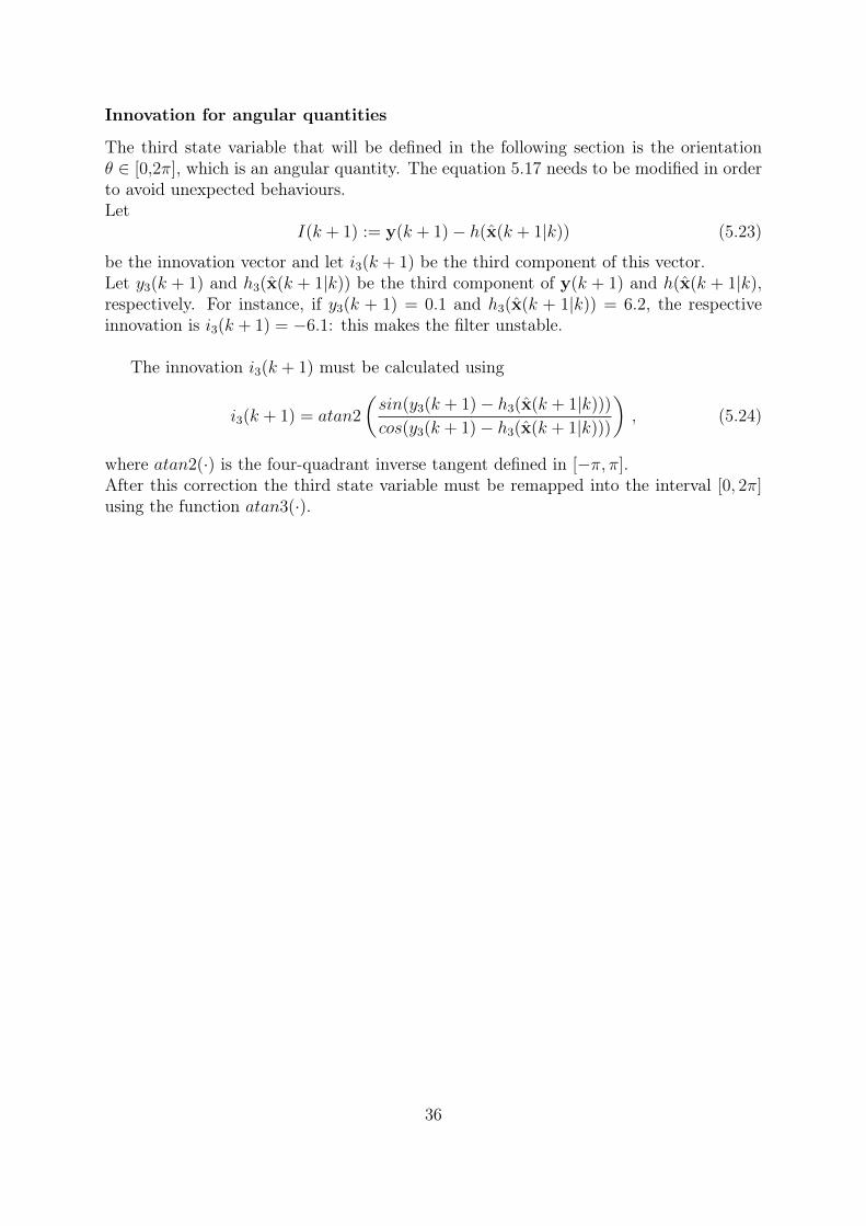
Innovation for angular quantities

The third state variable that will be defined in the following section is the orientationθ ∈ [0,2π], which is an angular quantity. The equation 5.17 needs to be modified in orderto avoid unexpected behaviours.Let

I(k + 1) := y(k + 1)− h(x(k + 1|k)) (5.23)

be the innovation vector and let i3(k + 1) be the third component of this vector.Let y3(k + 1) and h3(x(k + 1|k)) be the third component of y(k + 1) and h(x(k + 1|k),respectively. For instance, if y3(k + 1) = 0.1 and h3(x(k + 1|k)) = 6.2, the respectiveinnovation is i3(k + 1) = −6.1: this makes the filter unstable.

The innovation i3(k + 1) must be calculated using

i3(k + 1) = atan2

(sin(y3(k + 1)− h3(x(k + 1|k)))

cos(y3(k + 1)− h3(x(k + 1|k)))

), (5.24)

where atan2(·) is the four-quadrant inverse tangent defined in [−π, π].After this correction the third state variable must be remapped into the interval [0, 2π]using the function atan3(·).

36

5.3.2 Sensor fusion using visual and odometry information

This section introduces a model for the sensor fusion using the pose calculated by thenode datamatrix-pose-pub, as discussed in the chapter 4 and using the the speed s(·)and the steering angle ψ(·) published by the atlasmv-base node on the topic atlasmv-base/AtlasmvStatus1.

Model 1: equations

Let

x(t) =

x(t)y(t)θ(t)s(t)ψ(t)

(5.25)

be the state vector.The f(·) function is defined as:

f(x(t)) =

s(t) cos θ(t)s(t) sin θ(t)

s(t) tan(ψ(t))1l

00

, (5.26)

where the components 1, 2, 3 are the continuous equivalent of the 5.8 and the components4 and 5 are set to zero because the acceleration s(·) and the steering angular velocityψ(·) are not measurable without an IMU. The dynamic of the components 4 and 5 isdetermined by the process noise.

Since we have two different sources of information, there are also two observationfunctions:

hv(x(t)) =

x(t)y(t)θ(t)

, ha(x(t)) =

[s(t)ψ(t)

], (5.27)

where subscript v is for vision and a is for AtlasMV.

The Jacobian matrices are defined as:

Hv(x(tk)) =

1 0 0 0 00 1 0 0 00 0 1 0 0

, Ha(x(tk)) =

[0 0 0 1 00 0 0 0 1

], (5.28)

and the sampled state equation is defined as:

ftk(x(tk|tk)) =

x(tk) + s(tk)∆tk cos(θ(tk))y(tk) + s(tk)∆tk sin(θ(tk))θ(tk) + s(tk)∆tk tan(ψ(tk))

1l

00

, (5.29)

1More details about this node are discussed in chapter 6.

37

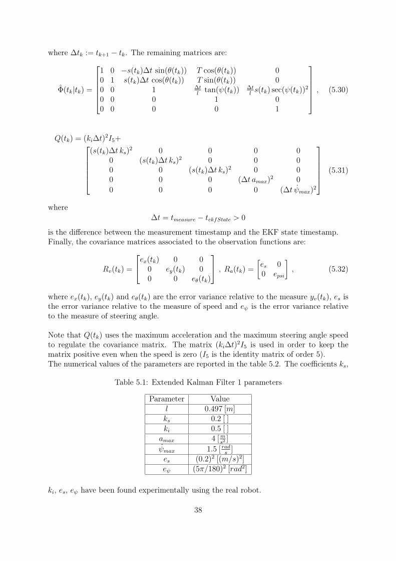
where ∆tk := tk+1 − tk. The remaining matrices are:

Φ(tk|tk) =

1 0 −s(tk)∆t sin(θ(tk)) T cos(θ(tk)) 00 1 s(tk)∆t cos(θ(tk)) T sin(θ(tk)) 00 0 1 ∆t

ltan(ψ(tk))

∆tls(tk) sec(ψ(tk))

2

0 0 0 1 00 0 0 0 1

, (5.30)

Q(tk) = (ki∆t)2I5+

(s(tk)∆t ks)2 0 0 0 0

0 (s(tk)∆t ks)2 0 0 0

0 0 (s(tk)∆t ks)2 0 0

0 0 0 (∆t amax)2 0

0 0 0 0 (∆t ψmax)2

(5.31)

where∆t = tmeasure − tekfState > 0

is the difference between the measurement timestamp and the EKF state timestamp.Finally, the covariance matrices associated to the observation functions are:

Rv(tk) =

ex(tk) 0 00 ey(tk) 00 0 eθ(tk)

, Ra(tk) =

[es 00 epsi

], (5.32)

where ex(tk), ey(tk) and eθ(tk) are the error variance relative to the measure yv(tk), es isthe error variance relative to the measure of speed and eψ is the error variance relativeto the measure of steering angle.

Note that Q(tk) uses the maximum acceleration and the maximum steering angle speedto regulate the covariance matrix. The matrix (ki∆t)

2I5 is used in order to keep thematrix positive even when the speed is zero (I5 is the identity matrix of order 5).The numerical values of the parameters are reported in the table 5.2. The coefficients ks,

Table 5.1: Extended Kalman Filter 1 parameters

Parameter Valuel 0.497 [m]ks 0.2 [ ]ki 0.5 [ ]amax 4 [m

s2]

ψmax 1.5 [ rads

]es (0.2)2 [(m/s)2]eψ (5π/180)2 [rad2]

ki, es, eψ have been found experimentally using the real robot.

38

This model has been implemented in MATLAB and used with the robot (both with realone and with a robot that was simulated using Gazebo). Its implementation is thoroughlydescribed in the chapter 6.

5.3.3 Sensor fusion using visual, odometry and inertial informa-tion

This section introduces a model for the sensor fusion in which an IMU (inertial measurementsunit) is also used. An additional sensor can be very useful both to increase the redun-dancy of the system and to increase the accuracy of the pose estimation.Moreover, the redundancy of information opens to the possibility of identifying some pa-rameters of the model. For instance, the model proposed in this section can identify andcorrect a proportional error in the speed measurement.

Since the IMU wasn’t available, this model hasn’t been used with the real robot. Itsvalidity was nonetheless studied and clearly proven through simulations.

Model 2: equations

In order to simplify the analysis, the discrete-time model have reported assumes that thevariables are sampled at a fixed sample time T .Let

x(k) =

x(k)y(k)θ(k)s(k)ψ(k)a(k)ω(k)sg(k)

(5.33)

be the state vector, where:

• a(k) is the acceleration along xr axis;

• ω(k) is the angular velocity around zr axis;

• sg(k) is the time-varying coefficient relative to a multiplicative error in speed mea-surement.

39

The state equation is defined as:

fk(x(k)) =

x(k) +(s(t)T + a(k)T

2

2

)cos θ(k)

y(k) +(s(t)T + a(k)T

2

2

)sin θ(k)

θ(k) + T (s(k) tanψ(t)) 1lα + Tω(k)(1− α)

s(k) + a(k)Tψ(k)a(k)ω(k)sg(k)

, (5.34)

where α ∈ (0,1) is used to calculate a weighted mean between the orientation obtainedusing the steering angle and the speed:

θ(k + 1) = θ(k) + Ts(k) tanψ(k)1

l,

and the orientation calculated using angular velocity provided by the IMU:

θ(k + 1) = θ(k) + Tω(k) .

The observation function is:

h(x(k)) =[x(k) y(k) θ(k) s(k)sg(k) ψ(k) a(k) ω(k)

]T, (5.35)

where the s(k)sg(k) is used to model the fact that the measured speed is the real speeds(k) multiplied by a gain sg(k).

Assuming that the speed is estimated using an encoder attached to a wheel, this modelcan explain and correct those errors which are due to a wrong estimation of the wheeldiameter, which can be caused, for example, by the variable tire pressure.

The Jacobian matrices is defined as:

H(x(tk)) =

1 0 0 0 0 0 0 00 1 0 0 0 0 0 00 0 1 0 0 0 0 00 0 0 sg(k) 0 0 0 s(k)0 0 0 0 1 0 0 00 0 0 0 0 1 0 00 0 0 0 0 0 1 0

. (5.36)

40

The remaining matrices are:

Q(k) =

(0.1∆t)2 0 0 0 0 0 0 00 (0.1∆t)2 0 0 0 0 0 00 0 (0.1∆t)2 0 0 0 0 00 0 0 (20amax∆t)

2 0 0 0 0

0 0 0 0 (10ψmax∆t)2 0 0 0

0 0 0 0 0 (10∆t)2 0 00 0 0 0 0 0 (20∆t)2 00 0 0 0 0 0 0 0

,

(5.37)

Φ(k|k) =

1 0 −(s(k)∆t+ a(k)∆t2) sin θ(k) ∆t cos θ(k) 0 ∆t2 cos θ(k) 0 00 1 (s(k)∆t+ a(k)∆t2) cos θ(k) ∆t sin θ(k) 0 ∆t2 sin θ(k) 0 00 0 1 ∆t

ltanψ(k)α ∆t

lαs(k)(secψ(k))2 0 ∆t(1− α) 0

0 0 0 1 0 ∆t 0 00 0 0 0 1 0 0 00 0 0 0 0 0 0 0

, (5.38)

R(k) = diag {ex, ey, eθ, es, eψ, ea, eω} , ∆t := tk+1 − tk . (5.39)

Note 1 Q(k) has a less complex structure in comparison to the previous case, in orderto underline the impact of the IMU.Note 2 The variance of the error associated to the process sg(·) is zero because it hasbeen assumed that it is a constant, though not exactly known value, and that is ideallyequal to 1. Otherwise, if sg(·) is not constant but slowly variable, the associated variancecan be a small but non-zero value (for example sg(·) = 10−6). In order to initializecorrectly the filter, the state variable sg(0) must be set to 1 with an associated variancegrater then zero.

The numerical values of the parameters are reported in the table 5.2.

41

Table 5.2: Extended Kalman Filter 2 parameters

Parameter Valuel 0.497 [m]

amax 4 [ms2

]

ψmax 1.5 [ rads

]α 0.1 []es (0.2)2 [(m/s)2]eψ (5π/180)2 [rad2]ex (0.2)2 [m2]ey (0.4)2 [m2]eθ (15π/180)2 [rad2]ea 0.001 [(m/s2)2]eω 0.001 [(rad/s)2]

5.3.4 Model verification using Simulink

This subsection presents a simulation used to prove the effectiveness of the model pre-sented in the previous section.The simulator is based on a realistic car-like model with equation:

d

dt

x(t)y(t)s(t)θ(t)

=

s(t) cos θ(t)s(t) sin θ(t)

a(t)s(t) tan(uψ(t))1

l

. (5.40)

The acceleration has equation:

a(t) =

(PuT (t)

s(t)− ACds(t)2

)1

m, (5.41)

where

• A = 0.5m is the frontal area of the car;

• Cd = 0.3 is the drag coefficient;

• m = 100kg is the mass;

• l = 1m is the wheelbase length;

• uT (t) ∈ [−1,1] is the throttle position;

• uψ(t) ∈ [−0.3,0.3] is the steering angle;

• P = 150W is the engine power.

42

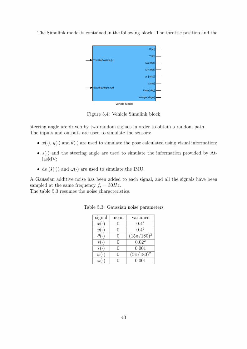
The Simulink model is contained in the following block: The throttle position and the

ThrottlePosition [-]

SteeringAngle [rad]

X [m]

Y [m]

DX [m/s]

DY [m/s]

ds [m/s2]

s [m/s]

theta [deg]

omega [deg/s]

Vehicle Model

Figure 5.4: Vehicle Simulink block

steering angle are driven by two random signals in order to obtain a random path.The inputs and outputs are used to simulate the sensors:

• x(·), y(·) and θ(·) are used to simulate the pose calculated using visual information;

• s(·) and the steering angle are used to simulate the information provided by At-lasMV;

• ds (s(·)) and ω(·) are used to simulate the IMU.

A Gaussian additive noise has been added to each signal, and all the signals have beensampled at the same frequency fs = 30Hz.The table 5.3 resumes the noise characteristics.

Table 5.3: Gaussian noise parameters

signal mean variancex(·) 0 0.42

y(·) 0 0.42

θ(·) 0 (15π/180)2

s(·) 0 0.022

s(·) 0 0.001ψ(·) 0 (5π/180)2

ω(·) 0 0.001

43

Simulations

The simulation parameters are as follows:

• the initial condition of the simulated robot have been set to zero (x(0) = y(0) =θ(0) = s(0) = ψ(0) = 0) and the coefficient sg (constant) is equal to 1.2;

• the initial values of the EKF have been set to zero, each variable with a variance0.1, except for sg, which is initialized to 1 with a variance of 0.152;

• the simulation time is 15s;

• the model with IMU corresponds to the model introduced in section 5.3.3 and themodel without IMU corresponds to the model introduced in section 5.3.2;

• Where applicable, the model without IMU uses the same parameters as the modelwith IMU, and it reads the real speed (not the real speed multiplied by 1.2).

The figure 5.5 shows the random path followed by the robot. The blue line representsthe real trajectory, and the green and black line the estimated trajectory without andwith IMU, respectively.Note that, as expected, the trajectory estimated using the IMU is less noisy.

Figure 5.5: Path traveled

44

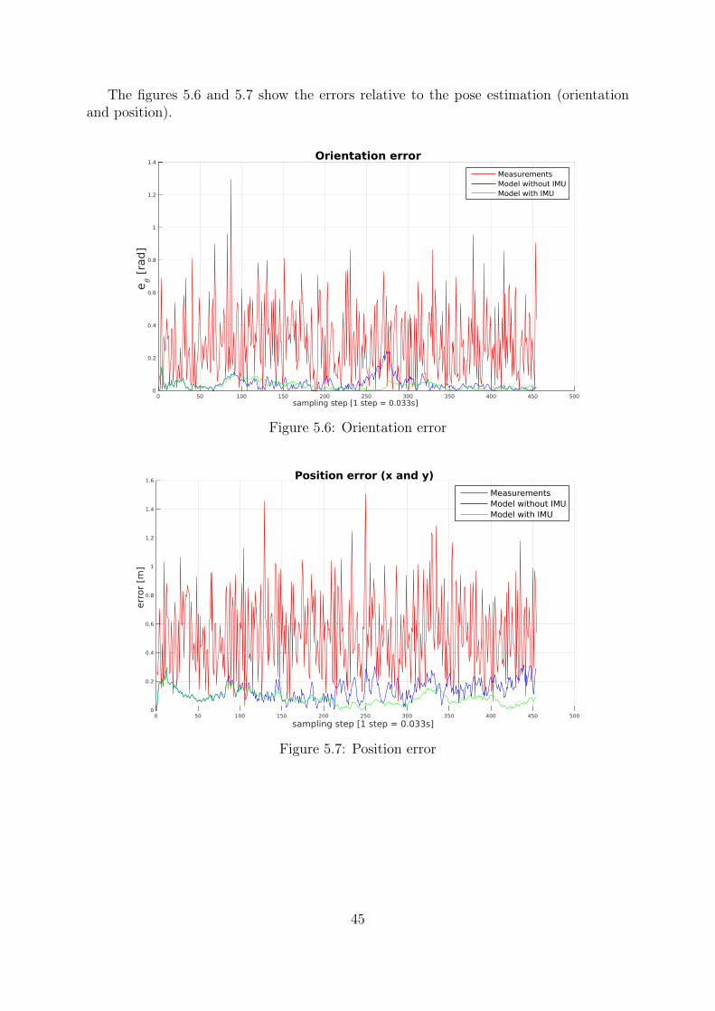
The figures 5.6 and 5.7 show the errors relative to the pose estimation (orientationand position).

Figure 5.6: Orientation error

Figure 5.7: Position error

45

The figures 5.8 and 5.9 show how the model with IMU can properly identify the pa-rameter sg and can also correct the speed estimation in less than 200 steps (about 6.6s).

Figure 5.8: Sg identification

Figure 5.9: Real vs estimated speed s(·)

46

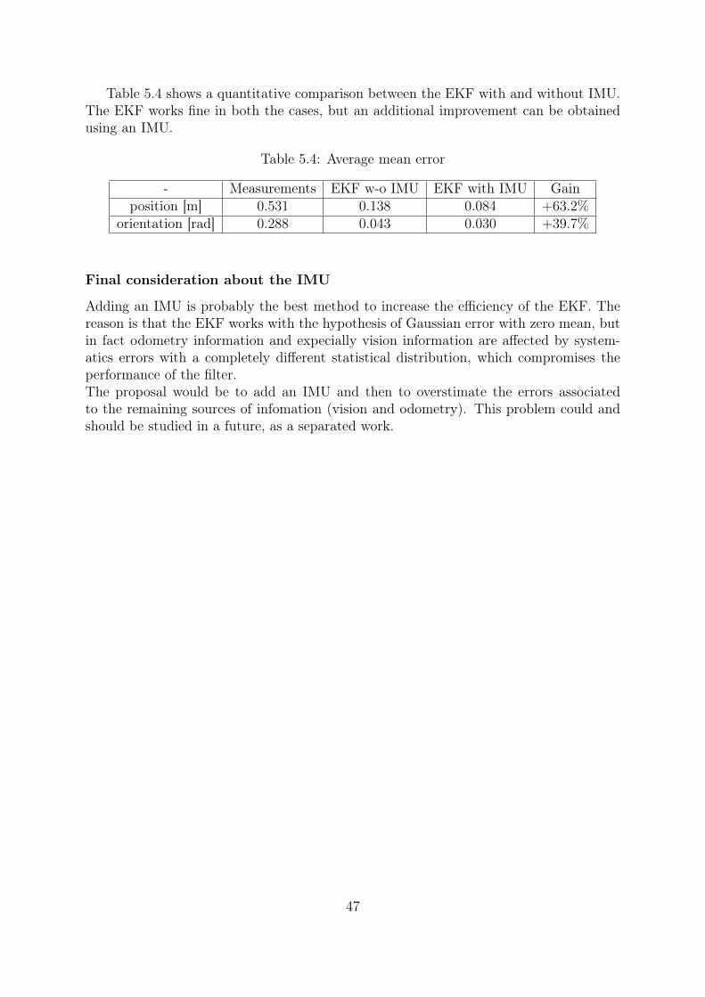
Table 5.4 shows a quantitative comparison between the EKF with and without IMU.The EKF works fine in both the cases, but an additional improvement can be obtainedusing an IMU.

Table 5.4: Average mean error

- Measurements EKF w-o IMU EKF with IMU Gainposition [m] 0.531 0.138 0.084 +63.2%

orientation [rad] 0.288 0.043 0.030 +39.7%

Final consideration about the IMU

Adding an IMU is probably the best method to increase the efficiency of the EKF. Thereason is that the EKF works with the hypothesis of Gaussian error with zero mean, butin fact odometry information and expecially vision information are affected by system-atics errors with a completely different statistical distribution, which compromises theperformance of the filter.The proposal would be to add an IMU and then to overstimate the errors associatedto the remaining sources of infomation (vision and odometry). This problem could andshould be studied in a future, as a separated work.

47

48

Chapter 6

Implementation in MATLAB

During the creation of an Extended Kalman Filter for ROS, it has been necessary to dealwith a problem connected to ROS and its implementation: ROS is not a real-time sys-tem and the messages are exchanged between nodes using the TCP/IP protocol. For thisreason, the non deterministic behaviour of ROS causes some uncertainty. Furthermore,the elaboration of visual information introduces a non-negligible delay. These problemshave been solved using a time-varying Extended Kalman Filter.The EKF has been implemented in MATLAB and connected to ROS using the RoboticsSystem ToolboxTM (RST) introduced in MATLAB r2015a.During the practical implementation of the filter two main problems have been high-lighted:

1. the measurements from the nodes atlasmv and datamatrix-pose-pub are aperiodicand can be received Out-of-Order;

2. MATLAB doesn’t provide any native mechanism for regulating the access to thevariables, like mutex (mutual exclusion)[27] does in C++. The multi-thread pro-gramming is also limited.

These problems have been partially solved using an algorithm specifically designed forMATLAB.

6.1 First proposed algorithmThe first proposed algorithm is the algorithm represented in fig. 6.1. This algorithm issubdivided in three different execution threads:

1. a first thread for the buffer management, for it to receive new measurements andstore them ordered by timestamp;

2. a second thread for updating the state x(tk|tk) when the contents of the bufferchanges;

3. a third thread that publishes the predicted pose of the robot ekf-robot-pose on aspecific ROS topic at a fixed publishing frequency fp (for example fp = 30Hz) andusing the last estimated state, as calculated by the second thread.

49

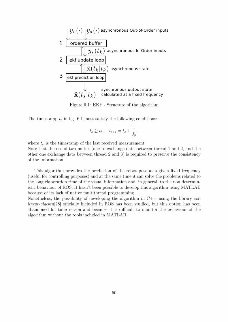
Figure 6.1: EKF - Structure of the algorithm

The timestamp ts in fig. 6.1 must satisfy the following conditions:

ts ≥ tk , ts+1 = ts +1

fp,

where tk is the timestamp of the last received measurement.Note that the use of two mutex (one to exchange data between thread 1 and 2, and theother one exchange data between thread 2 and 3) is required to preserve the consistencyof the information.

This algorithm provides the prediction of the robot pose at a given fixed frequency(useful for controlling purposes) and at the same time it can solve the problems related tothe long elaboration time of the visual information and, in general, to the non determin-istic behaviour of ROS. It hasn’t been possible to develop this algorithm using MATLABbecause of its lack of native multithread programming.Nonetheless, the possibility of developing the algorithm in C++ using the library ecl-linear-algebra[28] officially included in ROS has been studied, but this option has beenabandoned for time reason and because it is difficult to monitor the behaviour of thealgorithm without the tools included in MATLAB.

50

6.2 Second proposed algorithmThe second algorithm has been redesigned taking into account the limitations of MATLAB.The buffer has been removed, and the second and third threads have been merged into asingle thread.The resulting pseudo code is:

1 initializeROS()2 initializeEKF()3 while 1 {4 if newDatamatrixVectorAvailable() == TRUE {5 msg = getNewDatamatrixVector()6 rawRobotPose = poseMsg2rawPoseEst(msg)7 rawRobotPose = forwardEulerCorrection(rawRobotPose)8 publishRaw(rawRobotPose)9 ekfState = ekfUpdate(rawRobotPose)10 }11 if newAtlasMsgAvailable() == TRUE {12 pose = getNewAtlasMsg()13 ekfState = ekfUpdate(pose)14 }15 currentTime = getCurrentTime()16 prediction = ekfPrediction(ekfState,currentTime)17 publishOnRos(prediction)18 sleep(20ms)19 }

This code runs on MATLAB and it can be seen as a single execution thread 1.

1In fact, the RST hides a low-level layer based on the Java implementation of ROS, which usesmultiple threads to manage the connections between ROS nodes.

51

Explanation of the code

ROS initialization

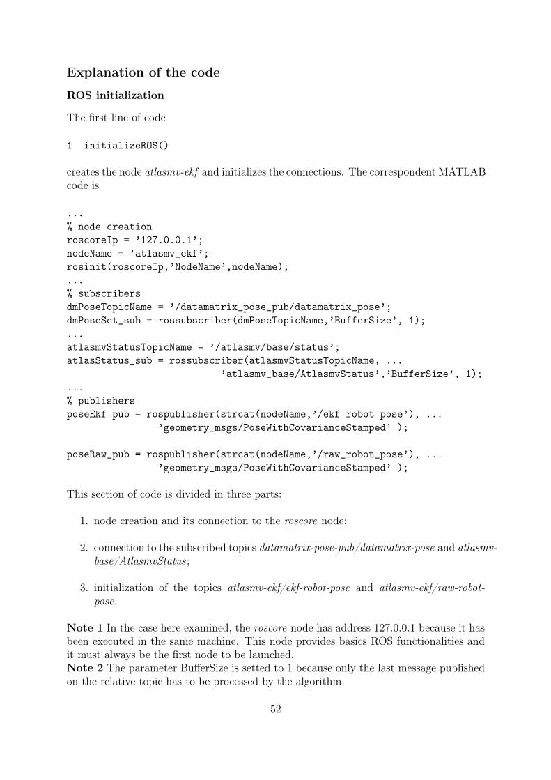
The first line of code

1 initializeROS()

creates the node atlasmv-ekf and initializes the connections. The correspondent MATLABcode is

...% node creationroscoreIp = ’127.0.0.1’;nodeName = ’atlasmv_ekf’;rosinit(roscoreIp,’NodeName’,nodeName);...% subscribersdmPoseTopicName = ’/datamatrix_pose_pub/datamatrix_pose’;dmPoseSet_sub = rossubscriber(dmPoseTopicName,’BufferSize’, 1);...atlasmvStatusTopicName = ’/atlasmv/base/status’;atlasStatus_sub = rossubscriber(atlasmvStatusTopicName, ...

’atlasmv_base/AtlasmvStatus’,’BufferSize’, 1);...% publishersposeEkf_pub = rospublisher(strcat(nodeName,’/ekf_robot_pose’), ...

’geometry_msgs/PoseWithCovarianceStamped’ );

poseRaw_pub = rospublisher(strcat(nodeName,’/raw_robot_pose’), ...’geometry_msgs/PoseWithCovarianceStamped’ );

This section of code is divided in three parts:

1. node creation and its connection to the roscore node;

2. connection to the subscribed topics datamatrix-pose-pub/datamatrix-pose and atlasmv-base/AtlasmvStatus ;

3. initialization of the topics atlasmv-ekf/ekf-robot-pose and atlasmv-ekf/raw-robot-pose.

Note 1 In the case here examined, the roscore node has address 127.0.0.1 because it hasbeen executed in the same machine. This node provides basics ROS functionalities andit must always be the first node to be launched.Note 2 The parameter BufferSize is setted to 1 because only the last message publishedon the relative topic has to be processed by the algorithm.

52

EKF initalization

The variable ekfState is a structure with the following fields:

1. wheelbase length l [m];

2. maximum velocity vmax [m/s];

3. maximum acceleration amax [m/s2];

4. maximum steering angle ψmax [rad];

5. maximum steering angle speed ψmax [rad/s];

6. state vector stateVec [[m][m][rad][m/s][rad]]T ;

7. covariance matrix covMatrix [unit of measurement derivable from stateVec];

8. timestamp of associated to the data structure timeStamp [s];

where parameters 1 to 5 are characteristics of the robot. Parameters 6 and 7 representthe state of the filter.

When the initialization step is finished, the function

2 initializeEKF()

waits for a message from datamatrix-pose-pub/datamatrix-pose and tries to calculate therobot pose (x, y, θ). The filter is initialized with the first valid pose (x, y, θ) that wascalculated. This approach requires that at least two data matrices are visible duringthe node initialization, otherwise the filter can’t be initialized and the main loop doesn’tstarts.

EKF loop

At line 3, the EKF starts to work.The code

4 if newDatamatrixVectorAvailable() == TRUE {5 msg = getNewDatamatrixVector()6 rawRobotPose = poseMsg2rawPoseEst(msg)7 rawRobotPose = forwardEulerCorrection(rawRobotPose)8 publishRaw(rawRobotPose)9 ekfState = ekfUpdate(rawRobotPose)10 }

checks if a new vector of data matrices has been published on the topic datamatrix-pose-pub/datamatrix-pose. If it has been received, the message is processed by the function:

6 rawRobotPose = poseMsg2rawPoseEst(msg)

53

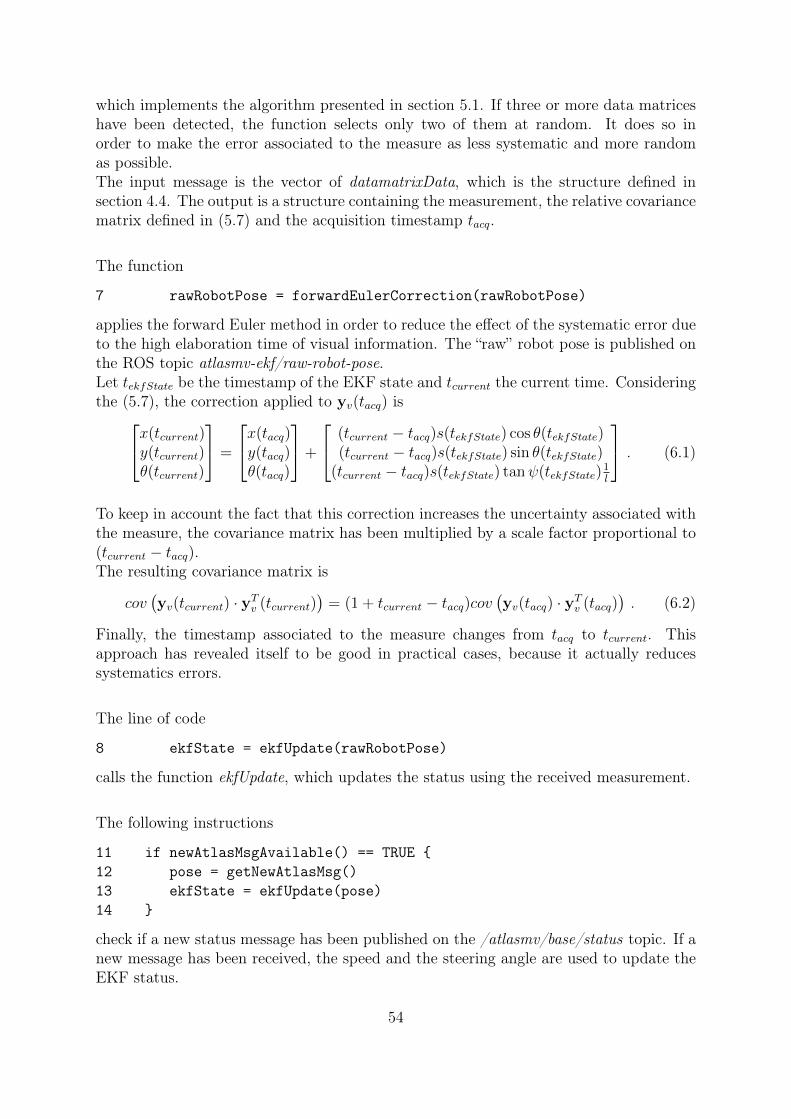
which implements the algorithm presented in section 5.1. If three or more data matriceshave been detected, the function selects only two of them at random. It does so inorder to make the error associated to the measure as less systematic and more randomas possible.The input message is the vector of datamatrixData, which is the structure defined insection 4.4. The output is a structure containing the measurement, the relative covariancematrix defined in (5.7) and the acquisition timestamp tacq.

The function

7 rawRobotPose = forwardEulerCorrection(rawRobotPose)

applies the forward Euler method in order to reduce the effect of the systematic error dueto the high elaboration time of visual information. The “raw” robot pose is published onthe ROS topic atlasmv-ekf/raw-robot-pose.Let tekfState be the timestamp of the EKF state and tcurrent the current time. Consideringthe (5.7), the correction applied to yv(tacq) isx(tcurrent)

y(tcurrent)θ(tcurrent)

=

x(tacq)y(tacq)θ(tacq)

+

(tcurrent − tacq)s(tekfState) cos θ(tekfState)(tcurrent − tacq)s(tekfState) sin θ(tekfState)

(tcurrent − tacq)s(tekfState) tanψ(tekfState)1l

. (6.1)

To keep in account the fact that this correction increases the uncertainty associated withthe measure, the covariance matrix has been multiplied by a scale factor proportional to(tcurrent − tacq).The resulting covariance matrix is

cov(yv(tcurrent) · yTv (tcurrent)

)= (1 + tcurrent − tacq)cov

(yv(tacq) · yTv (tacq)

). (6.2)

Finally, the timestamp associated to the measure changes from tacq to tcurrent. Thisapproach has revealed itself to be good in practical cases, because it actually reducessystematics errors.

The line of code

8 ekfState = ekfUpdate(rawRobotPose)

calls the function ekfUpdate, which updates the status using the received measurement.

The following instructions

11 if newAtlasMsgAvailable() == TRUE {12 pose = getNewAtlasMsg()13 ekfState = ekfUpdate(pose)14 }

check if a new status message has been published on the /atlasmv/base/status topic. If anew message has been received, the speed and the steering angle are used to update theEKF status.

54

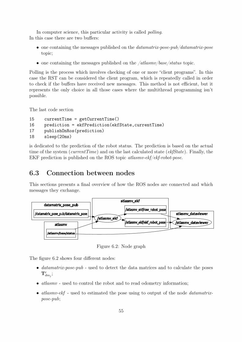
In computer science, this particular activity is called polling.In this case there are two buffers:

• one containing the messages published on the datamatrix-pose-pub/datamatrix-posetopic;

• one containing the messages published on the /atlasmv/base/status topic.

Polling is the process which involves checking of one or more “client programs”. In thiscase the RST can be considered the client program, which is repeatedly called in orderto check if the buffers have received new messages. This method is not efficient, but itrepresents the only choice in all those cases where the multithread programming isn’tpossible.

The last code section

15 currentTime = getCurrentTime()16 prediction = ekfPrediction(ekfState,currentTime)17 publishOnRos(prediction)18 sleep(20ms)

is dedicated to the prediction of the robot status. The prediction is based on the actualtime of the system (currentTime) and on the last calculated state (ekfState). Finally, theEKF prediction is published on the ROS topic atlasmv-ekf/ekf-robot-pose.

6.3 Connection between nodesThis sections presents a final overview of how the ROS nodes are connected and whichmessages they exchange.

Figure 6.2: Node graph

The figure 6.2 shows four different nodes:

• datamatrix-pose-pub - used to detect the data matrices and to calculate the posesTrdmj

;

• atlasmv - used to control the robot and to read odometry information;

• atlasmv-ekf - used to estimated the pose using to output of the node datamatrix-pose-pub;

55

• atlasmv-dataviewer - used to collect and visualize data.

The nodes datamatrix-pose-pub and atlasmv-ekf have already been discussed respectivelyin chapter 4 and in chapter 6.

The node atlasmv has been developed by the Laboratory for Automation and Roboticsof the University of Aveiro. This node provides a ROS interface for the robot.A message containing the status of the robot is published on a topic called atlasmv-base-status.This particular message is called AtlasmvStatus and it has the following structure:

Header headerfloat64 brakefloat64 dirfloat64 speedfloat64 xfloat64 yfloat64 orientationfloat64 distance_traveledint32 turnrightint32 turnleftint32 headlightsint32 taillightsint32 reverselightsint32 cross_sensorint32 vert_signint32 errors

When the node atlasmv-ekf receives this type of message, it extracts the timestamp (fromthe Header), the speed s(·) and the steering angle dir ψ(·).Header is a standard ROS message with the following structure:

uint32 seqtime stampstring frame_id

where seq is a sequential number, stamp is the timestamp and frame-id is an optionalstring.

Finally, the node atlasmv-dataviewer is created using MATLAB and it is used only tocollect and analyse data.

56

Chapter 7

Experimental results

This chapter presents the experimental results obtained using AtlasMV and its simu-lated version in Gazebo. Using the real robot, only qualitative considerations could beexpressed, since it wasn’t possible to measure the real position of the robot.On the contrary, through Gazebo it was possible to perform a quantitative analysis:the robot pose can be obtained reading the messages published by Gazebo on the topic/ackermann-vehicle/gazebo/model-states, which contains a vector of poses, one pose foreach object included in the simulated world.

7.1 Test environmentFigure 7.1 shows 21 data matrices generated and positioned inside the LAR. In order torecreate a similar scenario, the same data matrices have been included in the simulator.

Figure 7.1: Data matrices positioned inside the LAR.

57

The figure 7.2 shows the simulated robot, the data matrices and the simulated cam-eras outputs (front and rear cameras).For hardware limitations1, cameras output have been limited to a VGA resolution (640x480pixels) at 5 frames per second. A Gaussian noise with standard deviation 0.01 has beenadded to the generated frames.

Figure 7.2: Gazebo simulator

The tests with the real robot have been executed at a resolution of 1280x960 pixelsand at 10 frames per second. The exposure time has been manually set to 8 − 11ms(depending on light conditions). The detection algorithm doesn’t work if the image isblurred, because it is based on a corner detector (which is a gradient-based function).The low exposure time produces images with a low contrast but also with a low blureffect: many tests have been executed in order to find the best Libdmtx parameters.

Figure 7.3: Data matrices inside the LAR

1The processor Intel R© CoreTM i3-2310m wasn’t able to run the nodes and the simulator using twovirtual cameras at resolution of 1280x960 pixels.

58

7.2 Simulations using Gazebo

7.2.1 First simulation: “S” trajectory

In the first simulation, the robot was driven manually using an XboxTM 360 controller.The figure 7.4 shows the path travelled by the robot. There is a small offset between realposition (blu dots) and estimated position (black dots) (the measurements are indicatedwith the red crosses). Considering that this simulation was running in real time, thisproblem can be caused by the low MATLAB performance, which introduces a considerabledelay on data processing.

Figure 7.4: Gazebo simulation 1: trajectory

The figures 7.5 and 7.6 show a comparison between real and estimated position andbetween real and estimated orientation. It has been used the EKF without IMU intro-duced in chapter 6.

It is very interesting to note that the mean errors associated to this simulation arevery similar to the errors (table 5.4, reported below) obtained using the Simulink modelpresented in section 5.3.4.The table 7.1 shows a comparison between the mean error obtained with Simulink andthe one obtained with Gazebo.

59

Figure 7.5: Gazebo simulation 1: position error

Figure 7.6: Gazebo simulation 1: orientation error

In general, this level of precision can be considered acceptable for many real life appli-cations (the standard error is smaller than the robot dimension). A better performance

60

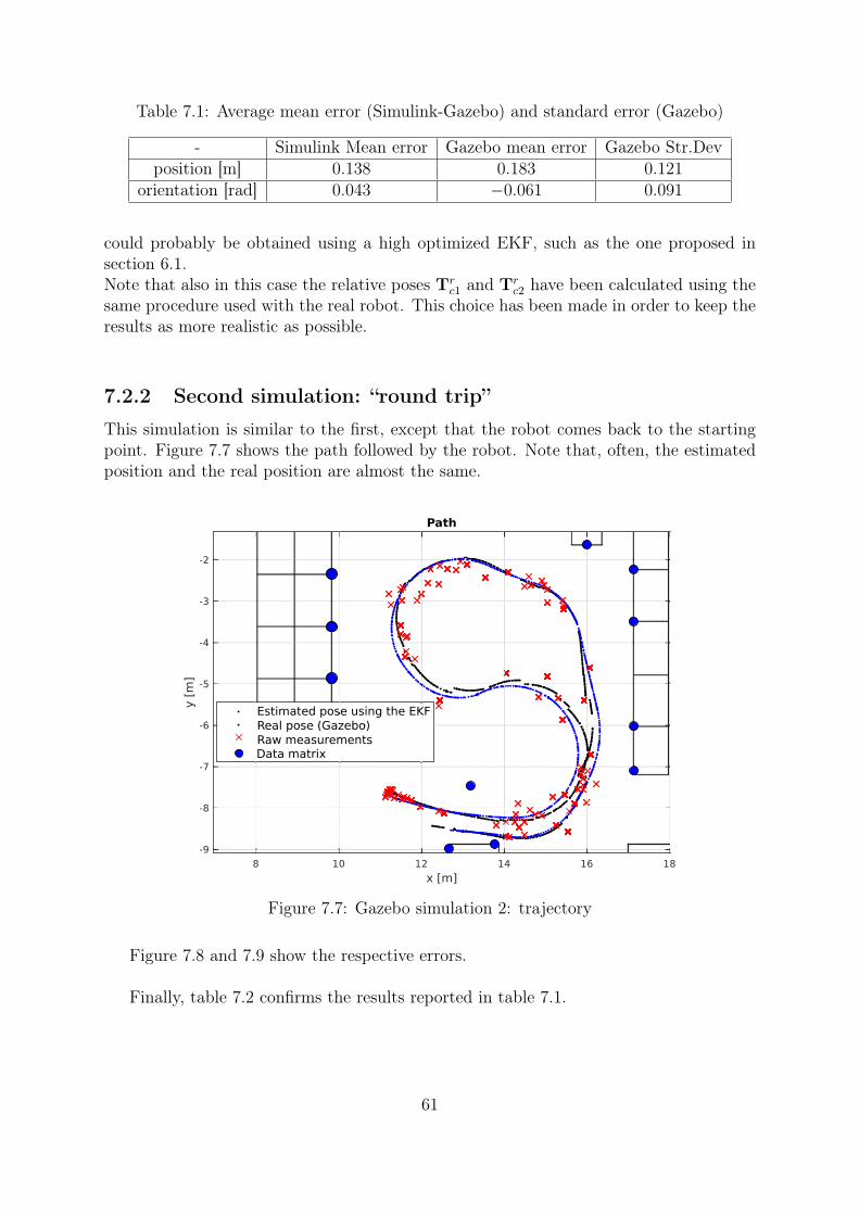
Table 7.1: Average mean error (Simulink-Gazebo) and standard error (Gazebo)

- Simulink Mean error Gazebo mean error Gazebo Str.Devposition [m] 0.138 0.183 0.121

orientation [rad] 0.043 −0.061 0.091

could probably be obtained using a high optimized EKF, such as the one proposed insection 6.1.Note that also in this case the relative poses Tr

c1 and Trc2 have been calculated using the

same procedure used with the real robot. This choice has been made in order to keep theresults as more realistic as possible.

7.2.2 Second simulation: “round trip”

This simulation is similar to the first, except that the robot comes back to the startingpoint. Figure 7.7 shows the path followed by the robot. Note that, often, the estimatedposition and the real position are almost the same.

Figure 7.7: Gazebo simulation 2: trajectory

Figure 7.8 and 7.9 show the respective errors.

Finally, table 7.2 confirms the results reported in table 7.1.

61

Figure 7.8: Gazebo simulation 2: position error

Figure 7.9: Gazebo simulation 2: orientation error

Table 7.2: Mean error and standard deviation

- Standard deviation Mean errorposition [m] 0.130 0.177

orientation [rad] 0.120 −0.081

7.2.3 Third simulation: straight trajectory

The third simulation shows the robot following a straight trajectory. Four data matriceshave been positioned, as shown in figure 7.10.

62

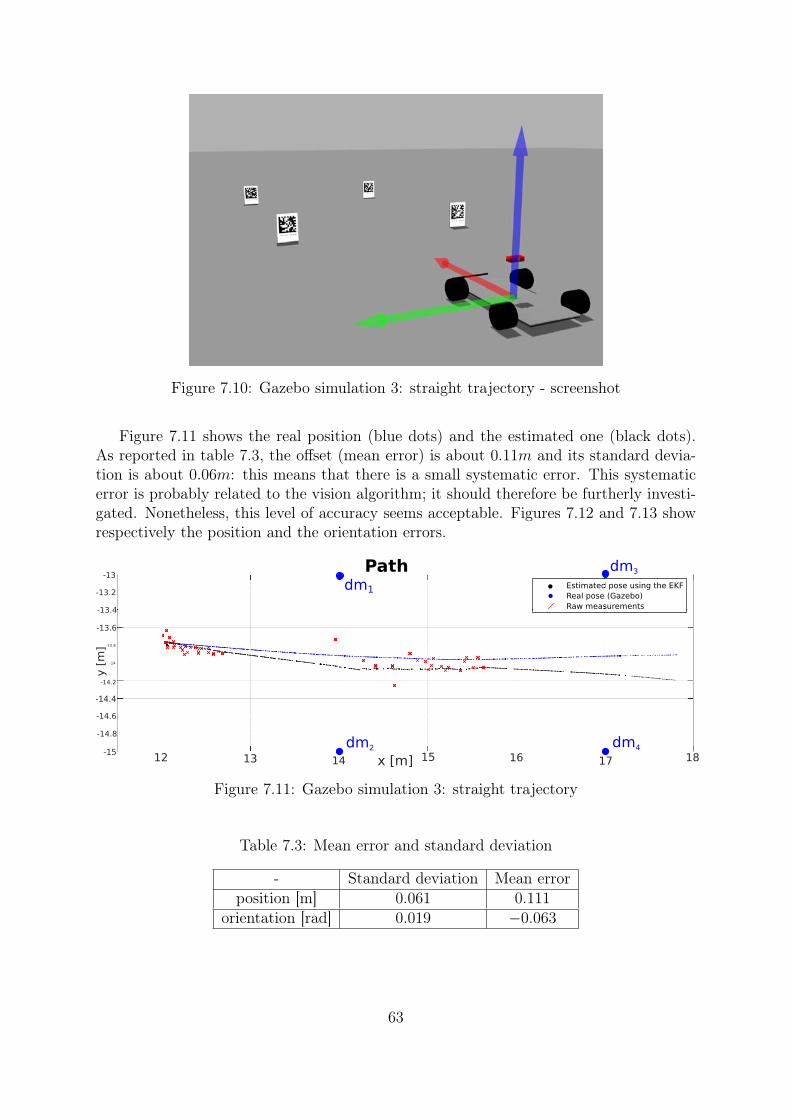
Figure 7.10: Gazebo simulation 3: straight trajectory - screenshot

Figure 7.11 shows the real position (blue dots) and the estimated one (black dots).As reported in table 7.3, the offset (mean error) is about 0.11m and its standard devia-tion is about 0.06m: this means that there is a small systematic error. This systematicerror is probably related to the vision algorithm; it should therefore be furtherly investi-gated. Nonetheless, this level of accuracy seems acceptable. Figures 7.12 and 7.13 showrespectively the position and the orientation errors.

Figure 7.11: Gazebo simulation 3: straight trajectory

Table 7.3: Mean error and standard deviation

- Standard deviation Mean errorposition [m] 0.061 0.111

orientation [rad] 0.019 −0.063

63

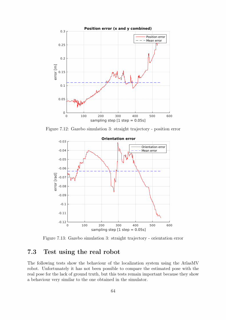
Figure 7.12: Gazebo simulation 3: straight trajectory - position error

Figure 7.13: Gazebo simulation 3: straight trajectory - orientation error

7.3 Test using the real robot

The following tests show the behaviour of the localization system using the AtlasMVrobot. Unfortunately it has not been possible to compare the estimated pose with thereal pose for the lack of ground truth, but this tests remain important because they showa behaviour very similar to the one obtained in the simulator.

64

7.3.1 First test: “S” trajectory

This simulation shows a “S” trajectory similar to the one obtained using Gazebo.

Figure 7.14: AtlasMV: “S” trajectory

The figure 7.14 shows the trajectory obtained using the AtlasMV robot with twoenabled cameras. The trajectory results less smooth if compared to the one obtainedwith Gazebo, and this for two reasons:

• difficulties in positioning the data matrices correctly;

• the speed estimation provided by AtlasMV is not accurate since the encoder isattached to the engine rotor and not to the wheel(s). Also, the differential introducesan additional error proportional to the steering angle.

Despite these problems, the result seems promising.

65

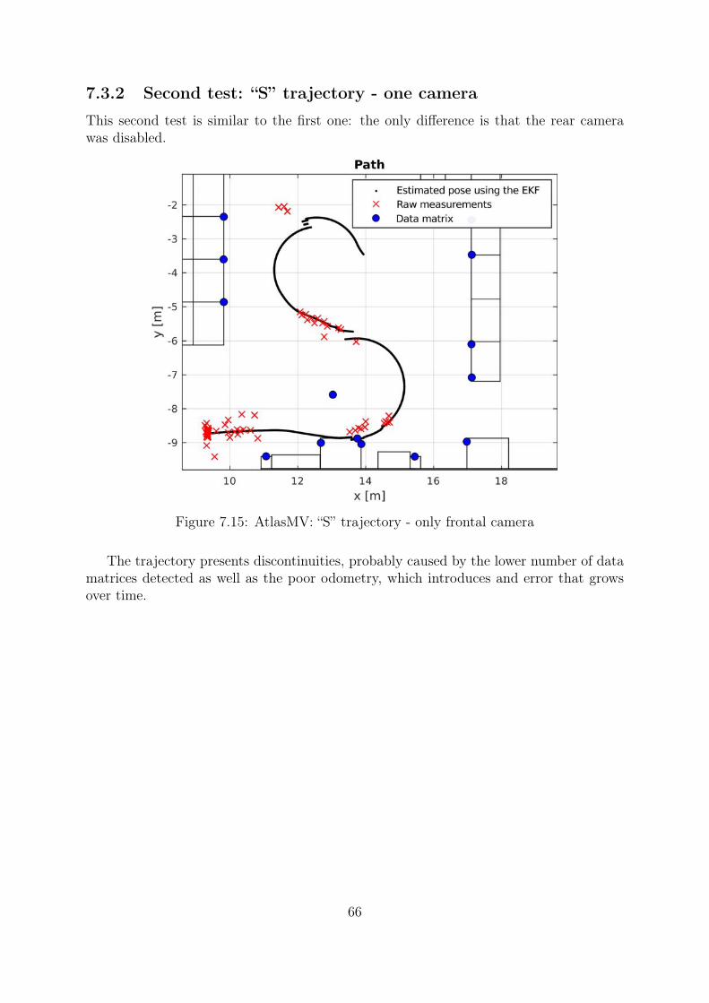
7.3.2 Second test: “S” trajectory - one camera

This second test is similar to the first one: the only difference is that the rear camerawas disabled.

Figure 7.15: AtlasMV: “S” trajectory - only frontal camera

The trajectory presents discontinuities, probably caused by the lower number of datamatrices detected as well as the poor odometry, which introduces and error that growsover time.

66

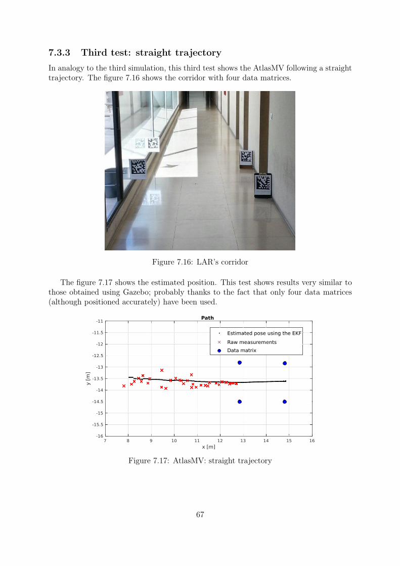
7.3.3 Third test: straight trajectory

In analogy to the third simulation, this third test shows the AtlasMV following a straighttrajectory. The figure 7.16 shows the corridor with four data matrices.

Figure 7.16: LAR’s corridor

The figure 7.17 shows the estimated position. This test shows results very similar tothose obtained using Gazebo; probably thanks to the fact that only four data matrices(although positioned accurately) have been used.

Figure 7.17: AtlasMV: straight trajectory

67

The tests with the real robot have confirmed that the localization system works asexpected.

The results does not seems as good as the results obtained with Gazebo, but this canbe easily explained keeping in consideration the following facts:

• every data matrix has been manually positioned with a given error;

• the map used was only an approximation of the real map;

• the odometry system was poor (encoders attached to the motors).

In this particular case, the main source of errors was determined by the measure of speedprovided by the robot (as already mentioned, the differential causes an error proportionalto the steering angle of the robot). Similar results to the ones obtained using Gazebo canbe obtained using a robot with a more accurate odometry system.

68

Chapter 8

Conclusions

The aim of this thesis was to implement an indoor localization system using visual infor-mation and passive markers. The obtained results are promising, but the performance ofthis type of system depends on many factors: detection algorithm, localization method,quality of the odometry and efficiency of the sensor fusion algorithm.

In chapter 3 the problem was discussed of how to encode efficiently the required in-formation. Moreover, a graphic tool has been developed in order the create the requiredmarkers. The encoding system was well dimensioned for this application: the resolutionof 0.1m was resulted sufficient (in practice it is difficult to position a data matrix withan error smaller than 0.1m).

Chapter 4 has described the perception algorithm based on the open source libraryLibdmtx, which was in general slow and not always stable. Despite these limitations, itwas accurate enough for this kind of application and it didn’t represent a bottleneck.The most delicate part of the operation has revealed itself to be the calibration: a badcalibration adds a systematic error to every single measurement.

Chapter 5 deals with the EKF as well as with the problem of sensor fusion. In orderto reduce the errors and also to eventually identify and correct systematic errors, the useof an inertial sensor was suggested. Since the systematic errors are the main problem ofthis technology, it would be advisable to further study this solution.

Chapter 6 deals with the implementation of the EKF and the problems connectedto its MATLAB implementation and its integration in ROS. The EKF has a big impacton the final accuracy of the localization system and its further optimization should beconsidered in future works.

In Chapter 7 have been introduced the experimental results obtained using the sim-ulator Gazebo and the robot AtlasMV. These tests show that the localization algorithmcan reach a precision smaller than 0.2m, which is acceptable for indoor autonomous nav-igation. On the other hand, the tests with the real robot show that the performance candegrade quickly if the system is not well calibrated, if the data matrices are not positionedexactly in the right position and if the robot odometry is not accurate.

69

An interesting continuation of this thesis would be to optimize the EKF, as suggestedin section 6.1. Also, it is crucial to tackle the problems caused by systematic errors. Thebest way to deal with this problem could be to add an inertial unit.

70

Bibliography

[1] R. E. Kalman, “A new approach to linear filtering and prediction problems,” ASMEJournal of Basic Engineering, 1960.

[2] C. Suliman, C. Cruceru, and F. Moldoveanu, “Mobile robot position estimation usingthe kalman filter,” Scientific Bulletin of the "Petru Maior" University of Tìrgu-Mureş, vol. 6, 2009.

[3] S. J. Julier and J. K. Uhlmann, “A new extension of the kalman filter to nonlinearsystems,” 1997, pp. 182–193.

[4] LAR - University of Aveiro. (2015) Atlas project. [Online]. Available:http://atlas.web.ua.pt/

[5] F. Caron, E. Duflos, D. Pomorski, and P. Vanheeghe, “Gps/imu datafusion using multisensor kalman filtering: Introduction of contextual aspects,”Inf. Fusion, vol. 7, no. 2, pp. 221–230, Jun. 2006. [Online]. Available:http://dx.doi.org/10.1016/j.inffus.2004.07.002

[6] J. M. Font-Llagunes and J. A. Batlle, “Consistent triangulation for mo-bile robot localization using discontinuous angular measurements,” Robot.Auton. Syst., vol. 57, no. 9, pp. 931–942, Sep. 2009. [Online]. Available:http://dx.doi.org/10.1016/j.robot.2009.06.001

[7] V. Pierlot and M. Van Droogenbroeck, “A new three object triangulation algorithmfor mobile robot positioning,” Trans. Rob., vol. 30, no. 3, pp. 566–577, Jun. 2014.[Online]. Available: http://dx.doi.org/10.1109/TRO.2013.2294061

[8] C. B. Madsen and C. S. Andersen, “Optimal landmark selection for triangulation ofrobot position,” Journal of Robotics and Autonomous Systems, vol. 13, pp. 277–292,1998.

[9] L. Carrão, “Sistema de visão pare guiamento de agv em ambiente industrial,” Mas-ter’s thesis, 2014.

[10] R. D’Andrea, “Guest editorial: A revolution in the warehouse: a retrospectiveon kiva systems and the grand challenges ahead.” IEEE T. AutomationScience and Engineering, vol. 9, no. 4, pp. 638–639, 2012. [Online]. Available:http://dblp.uni-trier.de/db/journals/tase/tase9.html# DAndrea12

[11] J. J. Enright, P. R. Wurman, and N. R. Ma, “Optimization and coordinated auton-omy in mobile fulfillment systems.”

71

[12] Willow Garage, University of Stanford. (2015) Ros: Robot operating system.[Online]. Available: http://www.ros.org/

[13] MATLAB. (2015) Robotics system toolbox. [Online]. Available:http://it.mathworks.com/products/robotics/

[14] M. Laughton. (2015) Libdmtx website. [Online]. Available:http://libdmtx.sourceforge.net/

[15] G. Bradski, “Opencv library,” Dr. Dobb’s Journal of Software Tools, 2000.

[16] MATLAB. (2015) Qt framework. [Online]. Available: http://www.qt.io/

[17] ISO, “Data matrix,” International Organization for Standardization, Geneva,Switzerland, ISO 16022:2000, 2000.

[18] ——, “Data matrix bar code symbology specification,” International Organizationfor Standardization, Geneva, Switzerland, ISO 16022:2006, 2006.

[19] I. S. Reed and G. Solomon, “Polynomial Codes Over Certain Finite Fields,” Journalof the Society for Industrial and Applied Mathematics, vol. 8, no. 2, pp. 300–304,1960. [Online]. Available: http://dx.doi.org/10.1137/0108018

[20] D. A. Forsyth and J. Ponce, Computer Vision: A Modern Approach. Prentice HallProfessional Technical Reference, 2002.

[21] R. I. Hartley and A. Zisserman,Multiple View Geometry in Computer Vision, 2nd ed.Cambridge University Press, ISBN: 0521540518, 2004.

[22] X.-S. Gao, X.-R. Hou, J. Tang, and H.-F. Cheng, “Complete solutionclassification for the perspective-three-point problem,” IEEE Trans. Pattern Anal.Mach. Intell., vol. 25, no. 8, pp. 930–943, Aug. 2003. [Online]. Available:http://dx.doi.org/10.1109/TPAMI.2003.1217599

[23] G. Bowman and P. Mihelich. (2015) Camera calibration - ros package. [Online].Available: http://wiki.ros.org/camera_calibration/

[24] A. Bradski, Learning OpenCV, [Computer Vision with OpenCV Library ; softwarethat sees], 1st ed. O‘Reilly Media, 2008.

[25] K. Levenberg, “A method for the solution of certain non-linear problems in leastsquares,” The Quarterly of Applied Mathematics, vol. 2, pp. 164–168, 1944.

[26] D. W. Marquardt, “An algorithm for least-squares estimation of nonlinearparameters,” SIAM Journal on Applied Mathematics, vol. 11, no. 2, pp. 431–441,1963. [Online]. Available: http://dx.doi.org/10.1137/0111030

[27] A. S. Tanenbaum, Modern Operating Systems, 3rd ed. Upper Saddle River, NJ,USA: Prentice Hall Press, 2007.

[28] D. Stonier. (2015) Ecl linear algebra - ros package. [Online]. Available:http://wiki.ros.org/ecl_linear_algebra

72