Embed Size (px)
Citation preview
1
The Energy Journal, Endogenous Technological Change and the Economics of Atmospheric Stabilisation Special Issue. Copyright ©2006 by the IAEE. All rights reserved.
* Potsdam Institute for Climate Impact Research, P.O. Box 60 12 03, Germany, E-mail: [email protected].
** DIW (German Institute for Economic Research) and Humboldt University Berlin, Germany, E-mail: [email protected].
*** Imperial College and Faculty of Economics, Cambridge University, United Kingdom, E-Mail: [email protected].
† Tyndall Centre and Faculty of Economics, University of Cambridge, Cambridge CB3 9DE, Sidgwick Avenue, United Kingdom, E-Mail: [email protected].
Induced Technological Change: Exploring its Implications for the Economics of Atmospheric Stabilization
Synthesis Report from the Innovation Modeling Comparison Project
Ottmar Edenhofer*, Kai Lessmann*, Claudia Kemfert**, Michael Grubb*** and Jonathan Köhler†
This paper summarizes results from ten global economy-energy-environment models implementing mechanisms of endogenous technological change (ETC). Climate policy goals represented as different CO
2 stabilization
levels are imposed, and the contribution of induced technological change (ITC) to meeting the goals is assessed. Findings indicate that climate policy induces additional technological change, in some models substantially. Its effect is a reduction of abatement costs in all participating models. The majority of models calculate abatement costs below 1 percent of present value aggregate gross world product for the period 2000-2100. The models predict different dynamics for rising carbon costs, with some showing a decline in carbon costs towards the end of the century. There are a number of reasons for differences in results between models; however four major drivers of differences are identified. First, the extent of the necessary CO
2 reduction which depends mainly on predicted baseline emissions,
determines how much a model is challenged to comply with climate policy. Second, when climate policy can offset market distortions, some models show that not costs but benefits accrue from climate policy. Third, assumptions about long-term investment behavior, e.g. foresight of actors and number of available
2 / The Energy Journal
investment options, exert a major influence. Finally, whether and how options for carbon-free energy are implemented (backstop and end-of-the-pipe technologies) strongly affects both the mitigation strategy and the abatement costs.
1. InTRoduCTIon
The Innovation Modeling Comparison Project (IMCP) aims to look at the impact of induced technological change (ITC) on the economics of stabiliz-ing carbon dioxide emissions at different levels. The IMCP is motivated by the conviction that endogenous technological change1 (ETC) is vital in modeling eco-nomic dynamics over the lengthy time scales required in climate policy analysis. Despite considerable progress in ETC research, significant discrepancies among models as well as uncertainties of model results still remain. The IMCP advances the understanding of ETC by assessing these discrepancies and analyzing their potential causes. This paper summarizes a quantitative model comparison experi-ment using a broad range of relevant models.
Two types of uncertainties contribute to the discrepancy of the results from different models. First, there is parameter uncertainty, referring to a lack of empirical knowledge to calibrate the parameters of a model to their “true” values. Parameter uncertainty implies an uncertainty of the predictions of any one model and discrepancies may result even in case of otherwise very similar models. Parameter uncertainty is addressed in model specific uncertainty analy-ses including sensitivity analysis and parameter studies, and modeling teams in the IMCP were encouraged to explore parameter uncertainty in the individual papers collected in this special issue. Second, there is structural uncertainty or model uncertainty, defined as the uncertainty arising from having more than one plausible model structure (Morgan and Henrion 1990, p. 67). In this paper, we address model uncertainty.
In general, model uncertainty may be reduced by eliminating possible model structures from the set of plausible models. One way of doing so is validat-ing models against empirical evidence to discriminate “better” models and con-sequently discard “bad” models. However, even “perfect validation” provides noHowever, even “perfect validation” provides no “perfect validation” provides noprovides no no proof that a model best explains reality. Alternatively, “Ockham�s razor” proposesAlternatively, “Ockham�s razor” proposes“Ockham�s razor” proposesOckham�s razor” proposes�s razor” proposess razor” proposes” proposes proposes that if another model explains the same empirical phenomena using less specific another model explains the same empirical phenomena using less specific or more intuitive assumptions and parameters, then it can be deemed preferable.then it can be deemed preferable.it can be deemed preferable.can be deemed preferable. preferable.. Yet to this date, the theoretical and empirical foundation of technological change to this date, the theoretical and empirical foundation of technological change, the theoretical and empirical foundation of technological changethe theoretical and empirical foundation of technological change within economics remains insufficient to allow for a sound evaluation of modelsfor a sound evaluation of modelsa sound evaluation of models according to Ockham�s razor. In other words, the uncertainties about the appropri-ate model structure remain.
1. We distinguish between endogenous and induced technological change: Technological change is endogenous (ETC) if its course is an outcome of economic activity within the model. Given an endogenous description, technological change in policy scenarios may exceed (or fall short of) its extent in the baseline, i.e. policies induce additional technological change which we refer to as ITC.
Our approach to model uncertainty involves identifying discrepancies in results of different models running the same scenarios, and investigating their origins. The analysis follows four steps: First, we classify the models according to their structure. Second, we assess discrepancies in a central model output, namely the impact of climate policy on the economy, or the “costs” of climate policy. Third, we analyze the different model dynamics leading to the discrepancies us-ing aggregated indicators of model behavior and drawing on structural informa-tion about the models. We measure the impact of technological change on these quantitative indicators,, ceteris paribus. Finally, we take a close look at the energy system as a major contributor to possible climate change.
The objective of this comparison is improved understanding of how and improved understanding of how and whether technological change matters. Technological change is a hotly debated issue because its impact on mitigation costs and mitigation strategies has political consequences. Recently, some models have been developed incorporating endog-enous technological change. Examples of the papers which compare these models in a qualitative way are Sijm (200�), Clarke and Weyant (2002), ��schel (2002), a qualitative way are Sijm (200�), Clarke and Weyant (2002), ��schel (2002), qualitative way are Sijm (200�), Clarke and Weyant (2002), ��schel (2002), Weyant and Olavson (1999), Grubb, K�hler and Anderson (2002), and K�hler et al. (2006), the latter includes an up to date survey of ETC in the literature.
The next section briefly summarizes the literature on modeling compari-son; in the third section, the participating models are characterized and a taxon-omy of models is provided. Section � outlines the method of comparison used in the IMCP. In Section 5, we analyze the impact of ITC on mitigation costs, mitiga-tion strategies, and energy mix. Section 6 offers some conclusions.
2. ModEl CoMPARISonS In ThE lITERATuRE
There is a broad literature on estimating the economic impact of climate change mitigation policies using models of various types. The Assessment Reports of the Intergovernmental Panel on Climate Change (IPCC) provide a comprehensive overview (IPCC 1996, 2001). Moreover, the Second and Third Assessment Reports (SAR and TAR) draw conclusions from comparative evaluations of these modeling studies. Among the original studies of model comparison, those of the Stanford Energy Modeling Forum (EMF) are particularly worth mentioning. This section briefly summarizes some of the key findings of previous model comparisons.
The SAR differentiates top-down (economic) and bottom-up (engineer-ing) models, further distinguishing Computable General Equilibrium models (CGE), optimizing models, and econometric macroeconomic models among the top-down approaches. Top-down and bottom-up models have been known to differ greatly in their estimates of the costs of mitigation policies. The authors of SAR note that this classification is increasingly misleading as efforts are being made to combine features from macro and CGE models, and to incorporate bottom-up technological features in top-down models. Furthermore, they conclude that differ-ent assumptions about the economic reality represented in the models, e.g. about the nature of market barriers, have a far greater impact on the results than the type
Induced Technological Change / 3
� / The Energy Journal
of the model. In their extended discussion of results from SAR, Hourcade and Robinson (1996) conclude that “there is no a-priori reason that the two model-ing approaches will give different results. Whether they [bottom-up and top-down models] do or not depends largely on their respective input assumptions”.
Two Economics Reports of the PEW Center on Global Climate Change summarize the economics of climate change policy and the role of technology (see Weyant 2000, Edmonds et al. 2000). Both studies review why model results differ. Weyant (2000) attributes the differences to variations mainly in the baselinevariations mainly in the baseline mainly in the baseline emission scenarios, different flexibilities regarding where, when, and which GHGregarding where, when, and which GHGwhere, when, and which GHG emissions are reduced, and whether or not benefits from avoided climate change are taken into account. Once the effects of these differences are separated, the re-sidual differences can be traced to substitution and technological change. EdmondsEdmonds et al. (2000) emphasize Hourcade and Robinson�s (1996) finding of the importance (2000) emphasize Hourcade and Robinson�s (1996) finding of the importance(2000) emphasize Hourcade and Robinson�s (1996) finding of the importance of assumptions underlying model design. Concerning the role of technological change, they note that technological change mitigates costs and occurs over long, they note that technological change mitigates costs and occurs over long they note that technological change mitigates costs and occurs over long time horizons. They stress that technological change can be induced by policies, and that including induced technological change is important, however difficult.
On discussions about why studies differ, TAR revisits the top-down ver- discussions about why studies differ, TAR revisits the top-down ver-s about why studies differ, TAR revisits the top-down ver- why studies differ, TAR revisits the top-down ver-sus bottom-up controversy. Top-down models are distinguished into CGE andto CGE and CGE and time-series-based econometric models, and TAR points out that the former typetype is arguably more suitable for describing long-run steady-state behavior, while the arguably more suitable for describing long-run steady-state behavior, while the latter models are more suitable for forecasting in the short-run. TAR also notes thatmodels are more suitable for forecasting in the short-run. TAR also notes that more suitable for forecasting in the short-run. TAR also notes thatin the short-run. TAR also notes thatthe short-run. TAR also notes that efforts are being made to eliminate these shortcomings (IPCC 2001, pp. 591).p. 591).. 591).
EMF 19 (200�) set out to understand how models being used for glob-al climate change policy analyses represent current and potential future energy technologies, and technological change. Weyant (200�) summarizes three main insights from the study: developing and implementing new energy technology is necessary for stabilizing atmospheric CO
2 concentration; the required transition
will be costly to implement, and implementation will take many decades; but costs may be moderated if it is possible to pursue many options, to phase in new technologies gradually, and if supporting policies start soon.
In an extensive survey of the recent literature, Sijm (200�) focuses on models that exhibit features of endogenous technological change.2 He separates bottom-up and top-down studies and finds major similarities in the outcomes of models in the former category, e.g. costs decline, the energy mix changes towards fast learners, and total abatement costs decline. Modeling studies in the latter category, however, show a wide diversity in outcomes with regard to the impact of induced technological change. He identifies variations in the following modelHe identifies variations in the following model features as possible explanations: ITC channels; optimization criteria; model: ITC channels; optimization criteria; model; optimization criteria; model optimization criteria; model; model model functions; calibration; spillovers; and also aggregation; number and type of policy; calibration; spillovers; and also aggregation; number and type of policy calibration; spillovers; and also aggregation; number and type of policy; spillovers; and also aggregation; number and type of policy spillovers; and also aggregation; number and type of policy; and also aggregation; number and type of policy and also aggregation; number and type of policy; number and type of policy number and type of policy instruments; and the time horizon.; and the time horizon. and the time horizon.
These modeling comparison exercises illuminate and outline reasonsilluminate and outline reasons reasons
2. For a recent collection of models incorporating ETC, see Vollebergh and Kemfert (2005).
why models differ in their cost estimates. Several studies list induced technologi-cal change as a good candidate for explaining some of these differences. However, the extent of its impact and the precise reasons as to how and why technological change matters remain unclear in many cases. Focusing on the effects of ITC, all participating modeling teams of the IMCP deliver scenarios in which technologi-cal change processes have been ‘switched off� and ‘switched on�. A comparison between these scenarios allows on the one hand, a quantitative assessment of tech-nological change and on the other hand, a further explanation of the underlying economic mechanisms that explain different model outputs.
3. ModEl ClASSIfICATIon
The models considered in this comparative study have two common aspects: they incorporate technological change in innovative ways and allow an: they incorporate technological change in innovative ways and allow anthey incorporate technological change in innovative ways and allow anhey incorporate technological change in innovative ways and allow an assessment of costs of global carbon dioxide mitigation. At the same time, a widea wide range of model types is represented in this project. Understanding the conceptions model types is represented in this project. Understanding the conceptions underlying the designs of different model types is necessary when comparing models within and across model types. In this section we give a summary of the concepts on which we base our discussion. We start with a general classification, which serves as a guideline for the brief introduction of the models that follows. As the major motivation for the design of many models as well as a key question in this study, we draw focus on the determination of the economic impact of cli-, we draw focus on the determination of the economic impact of cli- we draw focus on the determination of the economic impact of cli-e draw focus on the determination of the economic impact of cli- determination of the economic impact of cli-mate policies in terms of social costs, and recapitulate different concepts of costs, and recapitulate different concepts of costsrecapitulate different concepts of costs which are prominent in different model types..
3.1 Model Types in IMCP
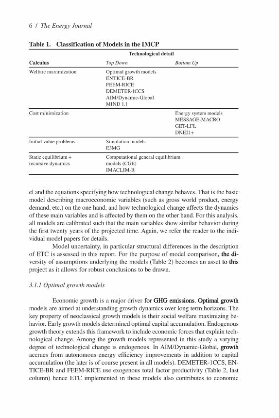
In Table 1, we differentiate four models types, mainly characterized by their calculus, i.e. the mathematical paradigm underlying the computation.
1. Optimal growth models – maximize social welfare intertemporally..2. Energy system models – minimize costs in the energy sector.3. Simulation models – solve initial value or boundary condition
problems (this includes econometric models, i.e. models which base a subset of their relationships on historical time series).
4. General equilibrium market models – balance demand and supply among multiple actors.
Many models in this study transcend the outlined categories. Whilst the modeling paradigm that underlies a model is useful for understanding its dynam-ics, we urge the reader to consult the individual papers for an in-depth discussion of the models.
These papers also include discussions of the model calibration and sen-sitivity analysis of crucial parameters. Model calibration is important to gauge the parameter uncertainties going into the models, and sensitivity analysis assesses the effect of these uncertainties. Model calibration includes equations of the basic mod-
Induced Technological Change / 5
6 / The Energy Journal
el and the equations specifying how technological change behaves. That is the basic model describing macroeconomic variables (such as gross world product, energy demand, etc.) on the one hand, and how technological change affects the dynamics of these main variables and is affected by them on the other hand. For this analysis, all models are calibrated such that the main variables show similar behavior during the first twenty years of the projected time. Again, we refer the reader to the indi-vidual model papers for details.
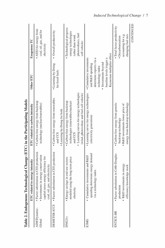
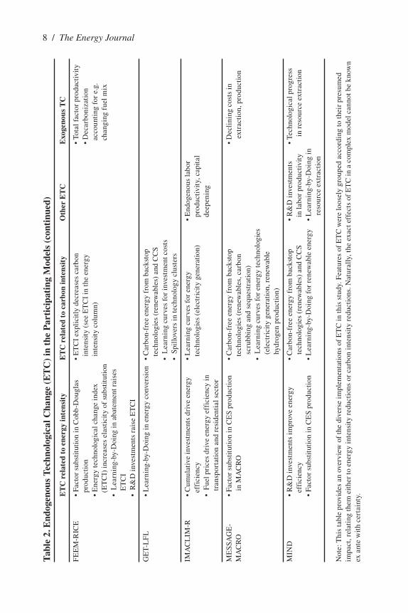
Model uncertainty, in particular structural differences in the description of ETC is assessed in this report. For the purpose of model comparison, the di-, the di- the di-versity of assumptions underlying the models (Table 2) becomes an asset to thisto this this project as it allows for robust conclusions to be drawn.
3.1.1 Optimal growth models
Economic growth is a major driver for GHG emissions. Optimal growthfor GHG emissions. Optimal growth GHG emissions. Optimal growth models are aimed at understanding growth dynamics over long term horizons. The key property of neoclassical growth models is their social welfare maximizing be-havior. Early growth models determined optimal capital accumulation. Endogenous growth theory extends this framework to include economic forces that explain tech-nological change. Among the growth models represented in this study a varying degree of technological change is endogenous. In AIM/Dynamic-Global, growth, growth growth accrues from autonomous energy efficiency improvements in addition to capital accumulation (the later is of course present in all models). DEMETER-1CCS, En-TICE-BR and FEEM-RICE use exogenous total factor productivity (Table 2, last column) hence ETC implemented in these models also contributes to economic
Table 1. Classification of Models in the IMCP Technological detail
Calculus Top Down Bottom Up
Welfare maximization Optimal growth models EnTICE-BR FEEM-RICE DEMETER-1CCS AIM/Dynamic-Global MInD 1.1
Cost minimization Energy system models MESSAGE-MACRO GET-�F� DnE21+
Initial value problems Simulation models E3MG
Static equilibrium + Computational general equilibrium recursive dynamics models (CGE) IMAC�IM-R
Induced Technological Change / 7
Tab
le 2
. End
ogen
ous
Tec
hnol
ogic
al C
hang
e (E
TC
) in
the
Par
tici
pati
ng M
odel
s
ET
C r
elat
ed t
o en
ergy
inte
nsit
y E
TC
rel
ated
to
carb
on in
tens
ity
oth
er E
TC
E
xoge
nous
TC
AIM
/Dyn
amic
-
• Fa
ctor
sub
stit
utio
n in
CE
S pr
oduc
tion
•
Car
bon-
free
ene
rgy
from
bac
ksto
p
• A
EE
I fo
r en
ergy
fro
m
Glo
bal
• In
vest
men
ts in
ene
rgy
cons
erva
tion
tech
nolo
gy (
nucl
ear/
rene
wab
les)
co
al, o
il, g
as, a
nd f
or
c
apit
al r
aise
s en
ergy
eff
icie
ncy
for
elec
tric
ity
c
oal,
oil,
gas,
and
ele
ctri
city
DE
ME
TE
R-1
CC
S
• Fa
ctor
sub
stit
utio
n in
CE
S pr
oduc
tion
•
Car
bon-
free
ene
rgy
from
ren
ewab
les
•
�ea
rnin
g-by
-Doi
ng
• O
vera
ll p
rodu
ctiv
ity
an
d C
CS
for
fos
sil f
uels
•
�ea
rnin
g-by
-Doi
ng f
or b
oth
Dn
E21
+
• E
nerg
y sa
ving
s in
end
-use
sec
tors
•
Car
bon-
free
ene
rgy
from
bac
ksto
p
• Te
chno
logi
cal p
rogr
ess
m
odel
ed u
sing
the
long
-ter
m p
rice
tech
nolo
gies
(re
new
able
s/nu
clea
r)
ener
gy te
chno
logi
es
elas
tici
ty.
an
d C
CS
(oth
er th
an w
ind,
•
�ea
rnin
g cu
rves
for
ene
rgy
tech
nolo
gies
ph
otov
olta
ics,
fue
l
(
win
d, p
hoto
volt
aic
and
fuel
cel
l veh
icle
)
ce
ll v
ehic
le)
E3M
G
• C
umul
ativ
e in
vest
men
ts a
nd R
&D
•
�ea
rnin
g cu
rves
for
ene
rgy
tech
nolo
gies
•
Cum
ulat
ive
inve
stm
ents
s
pend
ing
dete
rmin
e en
ergy
dem
and
(ele
ctri
city
gen
erat
ion)
and
R&
D s
pend
ing
via
a te
chno
logy
inde
x
de
term
ine
expo
rts
via
a
tech
nolo
gy in
dex
•
Inv
estm
ents
bey
ond
ba
seli
ne le
vels
trig
ger
a
Key
nesi
an m
ulti
plie
r ef
fect
En
TIC
E-B
R
• Fa
ctor
sub
stit
utio
n in
Cob
b-D
ougl
as
• C
arbo
n-fr
ee e
nerg
y fr
om g
ener
ic
•
Tota
l fac
tor
prod
ucti
vity
pr
oduc
tion
back
stop
tech
nolo
gy
•
Dec
arbo
niza
tion
• R
&D
inve
stm
ents
in e
nerg
y
• R
&D
inve
stm
ents
low
er p
rice
of
a
ccou
ntin
g fo
r e.
g.
effi
cien
cy k
now
ledg
e st
ock
ene
rgy
from
bac
ksto
p te
chno
logy
cha
ngin
g fu
el m
ix
CO
nT
InU
ED
� / The Energy JournalT
able
2. E
ndog
enou
s T
echn
olog
ical
Cha
nge
(ET
C)
in t
he P
arti
cipa
ting
Mod
els
(con
tinu
ed)
E
TC
rel
ated
to
ener
gy in
tens
ity
ET
C r
elat
ed t
o ca
rbon
inte
nsit
y o
ther
ET
C
Exo
geno
us T
C
FE
EM
-RIC
E
• Fa
ctor
sub
stit
utio
n in
Cob
b-D
ougl
as
• E
TC
I ex
plic
itly
dec
reas
es c
arbo
n
• To
tal f
acto
r pr
oduc
tivi
ty
p
rodu
ctio
n i
nten
sity
(se
e E
TC
I in
the
ener
gy
•
Dec
arbo
niza
tion
• E
nerg
y te
chno
logi
cal c
hang
e in
dex
i
nten
sity
col
umn)
acc
ount
ing
for
e.g.
(E
TC
I) in
crea
ses
elas
tici
ty o
f su
bsti
tuti
on
c
hang
ing
fuel
mix
• �
earn
ing-
by-D
oing
in a
bate
men
t rai
ses
E
TC
I
• R
&D
inve
stm
ents
rai
se E
TC
I
GE
T-�
F�
•
�ea
rnin
g-by
-Doi
ng in
ene
rgy
conv
ersi
on
• C
arbo
n-fr
ee e
nerg
y fr
om b
acks
top
t
echn
olog
ies
(ren
ewab
les)
and
CC
S
• �
earn
ing
curv
es f
or in
vest
men
t cos
ts
• S
pill
over
s in
tech
nolo
gy c
lust
ers
IMA
C�
IM-R
•
Cum
ulat
ive
inve
stm
ents
dri
ve e
nerg
y
• �
earn
ing
curv
es f
or e
nerg
y •
End
ogen
ous
labo
r
eff
icie
ncy
tec
hnol
ogie
s (e
lect
rici
ty g
ener
atio
n)
pro
duct
ivit
y, c
apit
al
•
Fue
l pri
ces
driv
e en
ergy
eff
icie
ncy
in
d
eepe
ning
tr
ansp
orta
tion
and
res
iden
tial
sec
tor
ME
SSA
GE
-
• Fa
ctor
sub
stit
utio
n in
CE
S pr
oduc
tion
•
Car
bon-
free
ene
rgy
from
bac
ksto
p
• D
ecli
ning
cos
ts in
M
AC
RO
in M
AC
RO
t
echn
olog
ies
(ren
ewab
les,
car
bon
ex
trac
tion
, pro
duct
ion
sc
rubb
ing
and
sequ
estr
atio
n)
• �
earn
ing
curv
es f
or e
nerg
y te
chno
logi
es
(e
lect
rici
ty g
ener
atio
n, r
enew
able
hydr
ogen
pro
duct
ion)
MIn
D
• R
&D
inve
stm
ents
impr
ove
ener
gy
• C
arbo
n-fr
ee e
nerg
y fr
om b
acks
top
• R
&D
inve
stm
ents
•
Tech
nolo
gica
l pro
gres
s
eff
icie
ncy
te
chno
logi
es (
rene
wab
les)
and
CC
S i
n la
bor
prod
ucti
vity
in r
esou
rce
extr
acti
on
•
Fact
or s
ubst
itut
ion
in C
ES
prod
ucti
on
• �
earn
ing-
by-D
oing
for
ren
ewab
le e
nerg
y •
�ea
rnin
g-by
-Doi
ng in
re
sour
ce e
xtra
ctio
n
not
e: T
his
tabl
e pr
ovid
es a
n ov
ervi
ew o
f th
e di
vers
e im
plem
enta
tion
s of
ET
C in
this
stu
dy. F
eatu
res
of E
TC
wer
e lo
osel
y gr
oupe
d ac
cord
ing
to th
eir
pres
umed
im
pact
, rel
atin
g th
em e
ithe
r to
ene
rgy
inte
nsit
y re
duct
ions
or
carb
on in
tens
ity
redu
ctio
ns. n
atur
ally
, the
exa
ct e
ffec
ts o
f E
TC
in a
com
plex
mod
el c
anno
t be
know
n ex
ant
e w
ith
cert
aint
y.
growth. In MInD, growth is fully endogenous. These models derive a first-best or a second-best social optimum and may be used as intertemporal social cost benefit analysis of mitigation strategies. First best models like MInD implicitly assume perfect markets and the implementation of optimal policy tools. InIn second best mod- best mod-els like FEEM-RICE market imperfections or sub-optimal policy tools are not re-are not re- not re-movable or modifiable. Policy of non-reproducible input factors instruments would be necessary. In other words, they may take so called no-regret options into account. In this case, the opportunity costs of climate protection can be lower or sometimes or sometimes sometimes even negative compared to the baseline, dependent on the design of climate policy.
In AIM/Dynamic-Global, ETC concerns energy efficiency (Masui et al. 2006). In addition to autonomous energy efficiency improvements, investments in energy conservation capital raise macroeconomic3 energy efficiency in the manufacturing sector, i.e. ETC affects the energy efficiency parameters in the production function which increases if the energy conservation capital stock in-creases faster than the output in the manufacturing sector. AIM/Dynamic-Global divides the world into six regions and describes regions with nine sectors which are mostly energy related.
FEEM-RICE (Bosetti et al. 2006) is modeled after nordhaus� regionalized integrated assessment model, RICE 99 (nordhaus and Boyer 2000). It differentiates eight world regions and computes the global solution by solving a non-cooperative nash game. ETC in FEEM-RICE is represented by an energy technological change index (ETCI) which is increased through R&D investments as well as by learn-ing-by-doing in carbon abatement. Its impact is twofold: ETCI affects the partial substitution coefficients in a Cobb-Douglas production function, shifting income shares from energy to capital. Secondly, ETCI decreases the macroeconomic carbon intensity. FEEM-RICE is presented in two parameterizations, FAST and S�OW, reflecting different assumptions about the speed of technological progress, its effec-tiveness and the crowding out effects between different types of investments.
EnTICE-BR (Popp 2006) is based on nordhaus� DICE model (nordhaus and Boyer 2000), hence it does not resolve regions. Among other modifications, Popp incorporates in his model, an R&D sector with two knowledge stocks. They are built in his model, an R&D sector with two knowledge stocks. They are built, an R&D sector with two knowledge stocks. They are built an R&D sector with two knowledge stocks. They are built up endogenously by R&D investments, one affecting macroeconomic energy effi-ciency and the other lowering the price of a generic backstop technologyand the other lowering the price of a generic backstop technology the other lowering the price of a generic backstop technologying the price of a generic backstop technology the price of a generic backstop technology�. Energy is produced either by this backstop technology, or from fossil fuels in a corresponding sector. Both EnTICE-BR and FEEM-RICE derive a second-best social optimum by simulating market behavior in an intertemporal optimization framework.
The model MInD (Edenhofer et al. 2006) is an intertemporal optimiza-tion model with a macroeconomic sector and four different energy sectors: re-source extraction, fossil-fuel based energy generation, a renewable energy source, and carbon-capturing and sequestration (CCS). The growth engine in the macro-
3. Here, we use the term macroeconomic to indicate an effect or process described at the macro level, e.g. described by one parameter for the economy.
�. Backstop technologies provide carbon-free energy and are not subject to any scarcities.
Induced Technological Change / 9
10 / The Energy Journal
economic sector is fueled by R&D investments in labor productivity and energy efficiency. There is no autonomous total factor productivity improvement. The investments in the different energy sectors are determined according to an inter-temporal optimal investment time path. MInD derives a first-best social optimum and therefore calculates the potential of ITC for reducing the costs of climate protection if market failures and social traps at the international level are resolved by appropriate policy measures.
DEMETER-1CCS models a dynamic economic system which is inter-temporally optimal for the representative household. The firms solve a per-period dynamic optimization problem, treating learning effects as external to the pro-duction decision level (Gerlagh 2006). Moreover, it comprises a composite good sector and different energy sectors for renewable energy sources (playing the role of a backstop-technology) and for fossil fuels. In the energy sector the costs are reduced through learning-by-doing.
3.1.2 Energy system models
Energy system models usually derive a cost-minimum sequence of en-ergy technologies for an exogenously given energy demand using linear program-ming. In more advanced versions, the energy technologies are improved by learn-ing-by-doing. The main advantages of this approach are the detailed depiction of the energy sector and the possibility of basing technological change on an en-gineering assessment of different technologies. Three energy system models are participating: DnE21+, GET-�F�, and MESSAGE-MACRO.
DnE21+ differentiates eight primary energy sources in 77 world regions (Sano et al. 2006). Technological change has an endogenous description for wind power, photovoltaics, and fuel-cell vehicles; exogenous assumptions about tech-nological change are made for other energy technologies. Energy demand in the end-use sectors is modeled using long-term price elasticities; gross world product (GWP) is exogenous to the model.
GET-�F� is a globally aggregated model differentiating eight primary energy sources (Hedenus et al. 2006). It includes a carbon capturing and sequestra-tion (CCS) option which is used with different fossil fuels as well as with biomass. GET-�F� implements cost minimization with limited foresight in a partial equi-librium (energy market), implying an elastic energy demand. ETC in GET-�F� is implemented in learning curves for investment costs of carbon-free technologies as well as energy conversion technologies, and spillovers in technology clusters.
MESSAGE-MACRO. The MESSAGE model describes the entire en-ergy system from resource extraction, through imports and exports, to conversion, transportation and end-use (Rao et al. 2006). �earning-by-doing is implemented for energy technologies. MESSAGE is solved in an iterative process with the economy model MACRO, allowing for some feedbacks between energy system and the macroeconomic environment, such as an impact on GWP.
3.1.3 Simulation and econometric models
We use the term simulation model to refer to models that start at a given state of the economy; then continue to calculate the next time step. In mathemati-cal terms, they solve initial value problems or boundary value problems given as systems of differential equations. Econometric simulation models are additionally based on time series data, i.e. the equations are estimated from data.
Econometric models are represented by the Tyndall Centre�s E3MG model (Barker et al. 2006). It is based on a post-Keynesian disequilibrium macro-economic structure with two sets of econometric equations (describing energy de-mand and export demand) estimated using Engle-Granger cointegration. E3MG differentiates 20 world regions modeled with input-output structures, �1 industrial sectors, 27 consumption categories, twelve fuels, and 19 fuel users.
3.1.4 General equilibrium models
General equilibrium models compute demand/supply equilibria in an economy modeled in distinct, interdependent sectors. Implicitly, households and firms within these sectors try independently to optimize their welfare and their profits, respectively. Computable General Equilibrium models (CGE) are promi-nent examples of this type. CGE models calculate static equilibria at each point in time prescribing some growth dynamic in between time steps, i.e. they are recur-sive dynamic. This guarantees not only that all markets are cleared but also that a Pareto-optimum is achieved. Sectoral resolution and the dynamics of relative prices are the main strengths of CGE models.
IMAC�IM-R is solved recursively but includes an endogenous growth en-gine that differs from standard CGE approaches (Crassous et al. 2006). The world is disaggregated into five regions, each made up by ten economic sectors. Cumulative investments drive both the energy efficiency and the labor efficiency at the same time. IMAC�IM-R represents formation of mobility needs through infrastructures and technical progress in vehicles. Three transportation sectors (air, sea, and terres-trial) are differentiated in which energy efficiency is driven by fuel prices. Addition-ally, energy technologies in electricity generation improve via learning-by-doing.
3.1.5 A comment on model types
Different modeling frameworks were created for different problems, with each model design tailored to address a specific set of questions. The charac-teristics of the modeling framework as well as the primary questions that guided its designs must be kept in mind when comparing the model results. Repetto and Austin (1997) note that macro and CGE models complement each other in pre-dicting short-term and long-term responses to a climate policy. Making models to predict century long economic behavior poses a great challenge in modeling frameworks that rely on past data or the present structure of the economy. Growth
Induced Technological Change / 11
12 / The Energy Journal
models using an optimizing framework allow endogenous savings and investment decisions with unlimited foresight while many recursive dynamic CGE models restrict optimizing behavior of its agents to a sequence of static equilibria. Hence, the time path of emissions and investments derived by most CGEs are not inter-temporally cost-effective. This lack of optimality is not a shortcoming of these models as they try to replicate the outcome of decentralized markets in which market imperfections are inherent. In contrast to recursive CGE models, an opti-mal economic growth model allows an understanding of transition paths and an assessment of what decentralized markets could achieve if appropriate policy in-struments were applied. On the other hand, most intertemporal economic growth models lack economic detail and offer only limited insights into sectoral dynam-ics. Energy system models focus on sectoral dynamics providing very detailed predictions. When restricted to the energy sector, they neglect feedbacks with the macroeconomic environment, e.g. the revaluation of capital. The integration of energy system models with macroeconomic models is a topical subject under scrutiny and a feature of several models in this study.
Three models, MInD, MESSAGE-MACRO and E3MG, adopt a hybrid approach, i.e. they combine features from different model designs to address the gap between them. MInD integrates technological detail similar to energy sys-tem models in the framework of a growth model. MESSAGE-MACRO adds an economic environment to an energy system model by iterating the models MES-SAGE and MACRO. E3MG includes a cost minimizing energy system sector within a Keynesian econometric model.
Finally, we note on the scope of the models. While all models are well calibrated, some models make very specific assumptions to explore special sce-narios. Three models in particular are explorative in character. First, IMAC�IM-R adopts a pessimistic view of technological change by assuming strong inertia and by neglecting carbon-free energy sources from backstop technologies. Second, AIM/Dynamic-Global focuses on the investment in energy-saving capital as a mitigation option, and largely neglects other options. As a consequence, economic growth cannot be decoupled from emissions. Third, FEEM-RICE is presented in a FAST version where especially optimistic assumptions are made about learning and the level of crowding-out.
4. METhodS of ModEl CoMPARISon
The following section outlines the IMCP approach of quantitative model comparison, specifically which scenarios were run, and which model outputs were reported. The effects of climate policies may be explored by comparing scenarios of climate protection with a business-as-usual scenario (baseline). In accordance with Article 2 of the UnFCCC which postulates stabilizing greenhouse gas con-centrations, we investigate climate policy scenarios with the goal of stabilized CO
2
concentration. We focus on carbon dioxide as the most influential GHG, defining three policy scenarios stabilizing CO
2 concentrations at levels of �50ppm, 500ppm,
and 550ppm, respectively. Where possible we also report results for a stabilization level of �00ppm. For this stabilization level the probability to meet the 2°C target is substantially increased (Hare and Meinshausen 200�). The 2°C target is per-ceived by some scientists and influential politicians, CEOs (like �ord Browne) and governmental bodies (like the EU Commission) as an interpretation of Article 2 of the UnFCCC. The concentration levels selected are somewhat arbitrary and serve to explore model responses to increasingly ambitious policies. As we prescribe a policy goal rather than a policy, model results represent a way of conforming to the policy goal and may guide the design of actual climate policy measures.
To assess the model response to climate policies and in particular the role of ITC, scenarios should ideally harmonize all other assumptions and also model calibration in order to isolate the effects of different implementations of ITC. It is known that the business-as-usual scenario has strong impact when evaluating the consequences of climate policies: assuming lower economic growth and therefore lower CO
2 emissions implies that climate protection poses a lesser challenge to the
economy. Where models prescribe gross world product (GWP) and/or emissions ex-ogenously, data from the Common PO�ES/IMAGE baseline (CPI) was used (Vuuren et al. 2003). However, harmonizing economic output and emissions in models which determine these numbers endogenously proves to be difficult if not impossible. Here, modeling teams have made an effort to calibrate their models to the CPI baseline, but there remain differences that must be taken in account when interpreting results.
Carbon dioxide concentration caps could not be imposed in models that do not include a carbon cycle submodel to translate emissions into concentrations. Such models either prescribe CO
2 emission paths corresponding to the selected
concentration levels exogenously, or constrain the overall centennial carbon bud-get. Differences in the implementation of carbon cycle models may imply that the same concentration level requires more stringent emission paths. Care was taken that the carbon cycle models showed good agreement.
4.1 Scenario definitions With and Without ITC
To assess the impact of ETC model output, stabilization scenarios were run with and without induced technological change. The baseline scenarios in IMCP comprise all components of endogenous technological change potentially incorpo-rated in the considered model. A policy scenario ‘with� induced technological change refers to a scenario in which additional endogenous technological change is induced by climate policy. In contrast to this, a policy scenario ‘without� induced techno-logical change means that climate policy cannot induce endogenous technological change beyond the baseline scenario. Therefore, in a policy scenario without ITC, technological change simply follows the time path of the baseline scenario as if it was given exogenously.5 A comparison between ‘with� and ‘without� induced tech-
5. The time paths of ETC related variables in the baseline simulation are stored and then prescribed as exogenous, fixed time series in this scenario.
Induced Technological Change / 13
1� / The Energy Journal
nological change measures the extent to which climate policy induces technological change in addition to baseline ETC. Table 3 summarizes these scenario definitions.
4.2 Model output and Indicators
The broad range of models is a key asset of this comparison, naturally comparable model outputs that are available in all models are of an aggregate nature. More specific outputs might allow deeper insights into some models but would exclude others. The selected model outputs (e.g. GWP, emissions, incre-mental costs of carbon, energy use, and the fuel mix) and the derived indicators (e.g. macroeconomic costs and sector costs, energy- and carbon intensity) reflect this trade off.
Despite the effort to harmonize assumptions and scenarios among mod-els, it remains a challenging task to determine why model results differ, i.e. to disentangle the role of ITC from other assumptions. In addition to the analysis offered in this paper, modelers were asked to elaborate on the calibration of their model and its sensitivities in their paper contributions to this special issue, thus providing a starting point to assess the assumptions underlying the model calibra-tion and their implications.
4.3 Concepts of Mitigation Costs
The SAR distinguishes four types of mitigation costs (IPCC 1996, p. 269). This taxonomy of costs provides a useful guide for the interpretation of results and is therefore recapitulated in the following:
1. Direct engineering costs of specific technical measures: These numbers provide some information about the costs of a mitigation measure or a specific technology. The cost estimates are mainly derived from engineering process-based studies of specific technologies. Examples include the costs of switching from coal to gas. In this model comparison, they are presupposed in all models.
2. Economic costs for a specific sector are computed in sector-specific models, which allow the integration of a multitude of mitigation measures, often in a partial equilibrium framework. For example, energy system models assess the sectoral costs of the energy sector.6
6. note that MESSAGE-MACRO goes beyond this by linking with the MACRO model.
Table 3. Summary of IMCP Scenario definitions.The baseline is a business-as-usual scenario. Technological change is determined endogenously.
Policy scenarios with ITC impose a policy goal of CO2 stabilization at three different levels (�50,
500, 550ppm CO2) or comparable
Policy scenarios without ITC impose the same policy goal but restrict technological change to the extent found in the baseline scenario
3. Macroeconomic costs reflect the impact of a given mitigation strategy on the level of the gross domestic product (GDP) and its components. At this level of analysis, feedbacks between sectors and the macroeconomic environment are accounted for. Such “general equilibrium effects” can be calculated by models which encompass either the whole economy, or coupled models of specific sectors and macro-economy. Thus, macroeconomic costs include the effects of engineering costs and sector-specific costs.
4. Welfare costs: The GDP variations, underlying the assessment of macroeconomic costs, do not provide an adequate measure of human welfare because the ultimate goal of economic activities is not producing GDP but allowing consumption of private and/or public goods and leisure. Mitigation policies, however, may increase investments and thus GDP while at the same time reducing consumption. Therefore, GDP is not a reasonable indicator for human welfare. However, per capita consumption is also a flawed indicator for welfare because human welfare is not always a linear function of per capita consumption. Therefore, most intertemporal optimization models assume in accordance with some empirical evidence that the utility index is an increasing function of per capita consumption, and marginal utility is decreasing with consumption. This implies that costs measured in per capita consumption are exaggerated or underestimated depending on the per capita consumption level. Moreover, the utility index depends also on the distributional issues and non-market traded goods and bads. Economists who rely on welfare theory may argue that the utility index could be modified according to fairness criteria and public goods. Therefore, this index could be used as a reliable indicator for human welfare.
Within IMCP, we analyze the impact of mitigation strategies on the sec-ond and third types of costs. Welfare implications along the lines of item � are not assessed explicitly because the models participating in IMCP do not share a common measure of welfare.
It seems worthwhile to note that all these cost concepts leave room for interpretation and may fuel a debate about the explanatory power of mitigation cost estimations. When GWP losses and consumption losses per capita are report-ed in absolute numbers, these are naturally large and may create the impression that mitigation is a costly option. Put into perspective as relative percentage of the net present value of the GWP in the business-as-usual scenario, mitigation may be seen as only postponing economic growth for several months. A simple thought experiment illustrates this point: Assume that GWP growth of 2% per year in the business-as-usual scenario. If mitigation policy lowered growth to 1.97%, GWP losses over the whole century discounted by 5 % would amount to 1%. In conse-
Induced Technological Change / 15
16 / The Energy Journal
quence, the annual GWP that would have been achieved in 2100 is now reached in 2101 (see Azar and Schneider 2002 for a similar argument). Does this imply that mitigation costs nearly nothing for humankind? One could argue that with these trillions of dollars the lives of millions of poor people could be rescued, e.g. by investing in clean water facilities. On the other hand, damages caused by non-action may destroy the rural habitats of millions of people elsewhere which also rarely count in terms of GWP. There is need for further investigation of the extent to which rapid climate change affects the welfare of people. Whilst acknowledg-ing that different social outcomes can be hidden behind an aggregated number like GWP and the limitations of this approach, some useful insights about the impact of ITC can be drawn using GWP. Clearly, a situation where GWP is increased because of ITC is preferable to a situation where climate policy reduces the op-portunities to invest in other desirable global projects.
In the context of IMCP we report GWP losses and consumption losses in terms of relative net present value which means that we measure the net present value losses between the business-as-usual scenario and the policy scenario and relate them to the net present value of GDP in the business-as-usual scenario. This allows a comparison of the cost estimations of different models.
When interpreting mitigation costs, it is necessary to recall that in the IMCP we compare mitigation costs at given stabilization levels. Some models, e.g. EnTICE-BR and FEEM-RICE estimate climate change impacts caused by specific stabilization levels. Therefore, the benefits of avoiding such impacts are reflected in the GWP losses in these models. In the IMCP, we inform the reader only about the mitigation costs of achieving a certain stabilization level irrespec-tive how much damages can be avoided by the predefined stabilization levels. In the cases of EnTICE-BR and FEEM-RICE the mitigation costs are reduced further by the damages caused at the specific stabilization level. Therefore, these GWP losses can be interpreted as net mitigation costs. In the following section we discuss the impact of technological change on these mitigation costs.
5. RESulTS And dISCuSSIon
This section presents the collected data as follows: First we outline and analyze the costs of achieving specific stabilization targets. Second, we analyze the necessary emission reductions in the different models in terms of their effect on carbon intensity, energy intensity, and gross world product. Third, the transfor-mation of the energy system which is a key challenge to meet the climate protec-tion targets is described and evaluated.
5.1 Mitigation Costs Within different Model Types
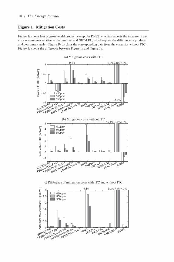
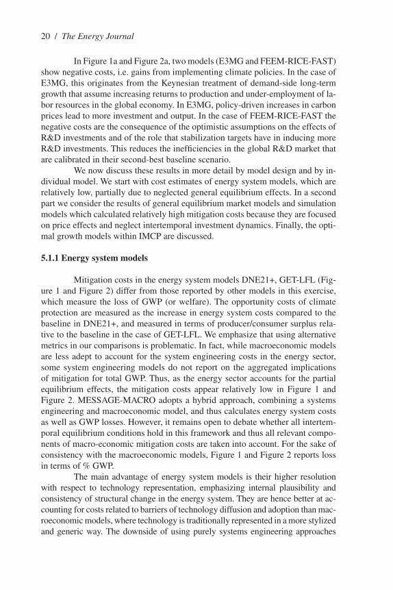
In this section we refer simultaneously to two different representations of mitigation costs. In both representations – Figure 1 and in Figure 2 – we show the mitigation costs as a loss of gross world product (GWP). Figure 1a shows mitigation
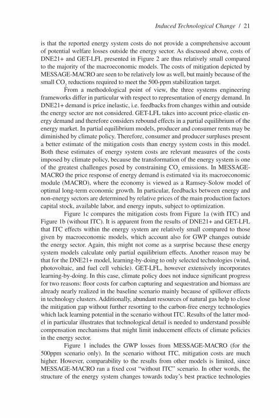
costs from different models relative to the respective baseline GWP in the case when technological change is switched on (cf. scenario definitions in Table 3). In Figure 1b the cost estimations are reported when technological change is switched off, Figure 1c indicates the additional mitigation costs for the scenarios without technological change, i.e. the differences between Figure 1a and Figure 1b. Figure 1c shows the potential to induce technological change in the different models: the larger the cost increase when ITC is switched off, the lower the potential of endogenous technologi-cal change incorporated in the implementation in that model. If a models incorpo-rated no endogenous technological change, Figure 1c would indicate no additional costs because costs with ITC would be the same as costs without ITC.
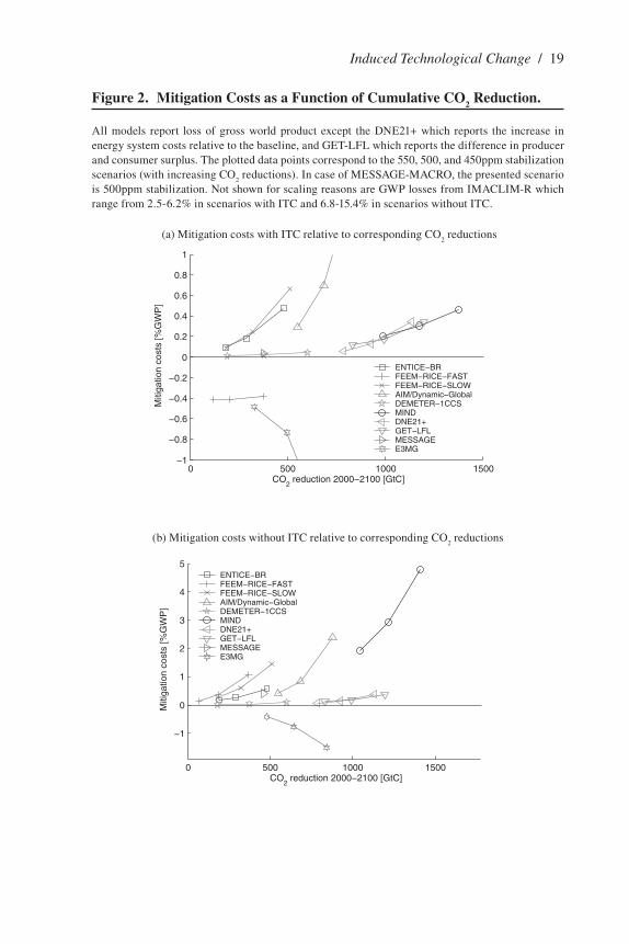
In Figure 2 the mitigation costs are shown as a function of the cumula-tive CO
2 reduction. The plotted data points correspond to the 550, 500 and �50
ppm stabilization scenario. The main purpose of Figure 2 is to relate costs to the mitigation gap which has to be overcome by the different models. In some models the costs are relatively low because of a small mitigation gap and not because of a strong impact of ITC on the costs. In all but two models, mitigation costs are computed as the difference in cumulated GWP (2000 to 2100) between baseline and policy scenarios, discounted at a rate of 5% and relative to (discounted) base-line GWP of the same time span.7 As there is no endogenous GWP in DnE21+ and GET-�F�, they present instead energy system costs and producer/consumer surplus in the energy sector, respectively.�
By plotting the costs at different stabilization levels against the corre-sponding cumulative CO
2 reductions (also 2000 to 2100), the costs are put into
perspective of the mitigation challenge that each model is confronted with in the policy scenarios.
The severity of the challenge is determined by the ‘mitigation gap‘, i.e. the difference between predicted business-as-usual emissions and admissible emissions in the policy scenario. Models tend to agree on the latter, which is a property of the carbon cycle modules in the models, but advocate various pre-dictions of business-as-usual GWP growth and CO
2 emissions. Consequently, so
called baseline effects have a strong influence on the results. Figure 2a depicts re-sults from scenarios with ITC; for the scenarios in Figure 2b, ITC was disabled.
With one exception (E3MG), the models agree about the trend of costs: lower concentration targets imply larger costs. Also, costs rise disproportionately with CO
2 reductions.
7. We use a 5% rate to discount GWP reductions from all models to make numbers comparable among models and to other studies in the literature. The rates of pure time preference used in models that anticipate future development vary: EnTICE-BR and FEEM-RICE use a 3% rate initially which declines over the course of the century; AIM/Dynamic-Global applies a �% discount rate; the rates of pure time preference are 3% and 1% in DEMETER-1CCS and MInD, respectively; the energy system models (DnE21+, GET-�F�, and MESSAGE-MACRO) use a 5% discount rate. There is no (macroeconomic) discounting in E3MG (except in the electricity sector) and IMAC�IM-R.
�. Surplus and energy system costs are converted to the same metric as the GWP losses, i.e. their difference between baseline and policy scenarios is presented relative to the present value of baseline GWP.
Induced Technological Change / 17
1� / The Energy Journal
figure 1. Mitigation Costs
Figure 1a shows loss of gross world product, except for DnE21+, which reports the increase in en-ergy system costs relative to the baseline, and GET-�F�, which reports the difference in producer and consumer surplus. Figure 1b displays the corresponding data from the scenarios without ITC. Figure 1c shows the difference between Figure 1a and Figure 1b.
(a) Mitigation costs with ITC
(b) Mitigation costs without ITC
c) Difference of mitigation costs with ITC and without ITC
Induced Technological Change / 19
figure 2. Mitigation Costs as a function of Cumulative Co2 Reduction.
All models report loss of gross world product except the DnE21+ which reports the increase in energy system costs relative to the baseline, and GET-�F� which reports the difference in producer and consumer surplus. The plotted data points correspond to the 550, 500, and �50ppm stabilization scenarios (with increasing CO
2 reductions). In case of MESSAGE-MACRO, the presented scenario
is 500ppm stabilization. not shown for scaling reasons are GWP losses from IMAC�IM-R which range from 2.5-6.2% in scenarios with ITC and 6.�-15.�% in scenarios without ITC.
(a) Mitigation costs with ITC relative to corresponding CO2 reductions
(b) Mitigation costs without ITC relative to corresponding CO2 reductions
20 / The Energy Journal
In Figure 1a and Figure 2a, two models (E3MG and FEEM-RICE-FAST) show negative costs, i.e. gains from implementing climate policies. In the case of E3MG, this originates from the Keynesian treatment of demand-side long-term growth that assume increasing returns to production and under-employment of la-bor resources in the global economy. In E3MG, policy-driven increases in carbon prices lead to more investment and output. In the case of FEEM-RICE-FAST the negative costs are the consequence of the optimistic assumptions on the effects of R&D investments and of the role that stabilization targets have in inducing more R&D investments. This reduces the inefficiencies in the global R&D market that are calibrated in their second-best baseline scenario.
We now discuss these results in more detail by model design and by in-dividual model. We start with cost estimates of energy system models, which are relatively low, partially due to neglected general equilibrium effects. In a second part we consider the results of general equilibrium market models and simulation models which calculated relatively high mitigation costs because they are focused on price effects and neglect intertemporal investment dynamics. Finally, the opti-mal growth models within IMCP are discussed.
5.1.1 Energy system models
Mitigation costs in the energy system models DnE21+, GET-�F� (Fig-ure 1 and Figure 2) differ from those reported by other models in this exercise, which measure the loss of GWP (or welfare). The opportunity costs of climate protection are measured as the increase in energy system costs compared to the baseline in DnE21+, and measured in terms of producer/consumer surplus rela-tive to the baseline in the case of GET-�F�. We emphasize that using alternative metrics in our comparisons is problematic. In fact, while macroeconomic models are less adept to account for the system engineering costs in the energy sector, some system engineering models do not report on the aggregated implications of mitigation for total GWP. Thus, as the energy sector accounts for the partial equilibrium effects, the mitigation costs appear relatively low in Figure 1 and Figure 2. MESSAGE-MACRO adopts a hybrid approach, combining a systems engineering and macroeconomic model, and thus calculates energy system costs as well as GWP losses. However, it remains open to debate whether all intertem-poral equilibrium conditions hold in this framework and thus all relevant compo-nents of macro-economic mitigation costs are taken into account. For the sake of consistency with the macroeconomic models, Figure 1 and Figure 2 reports loss in terms of % GWP.
The main advantage of energy system models is their higher resolution with respect to technology representation, emphasizing internal plausibility and consistency of structural change in the energy system. They are hence better at ac-counting for costs related to barriers of technology diffusion and adoption than mac-roeconomic models, where technology is traditionally represented in a more stylized and generic way. The downside of using purely systems engineering approaches
is that the reported energy system costs do not provide a comprehensive account of potential welfare losses outside the energy sector. As discussed above, costs of DnE21+ and GET-�F� presented in Figure 2 are thus relatively small compared to the majority of the macroeconomic models. The costs of mitigation depicted by MESSAGE-MACRO are seen to be relatively low as well, but mainly because of the small CO
2 reductions required to meet the 500-ppm stabilization target.
From a methodological point of view, the three systems engineering frameworks differ in particular with respect to representation of energy demand. In DnE21+ demand is price inelastic, i.e. feedbacks from changes within and outside the energy sector are not considered. GET-�F� takes into account price-elastic en-ergy demand and therefore considers rebound effects in a partial equilibrium of the energy market. In partial equilibrium models, producer and consumer rents may be diminished by climate policy. Therefore, consumer and producer surpluses present a better estimate of the mitigation costs than energy system costs in this model. Both these estimates of energy system costs are relevant measures of the costs imposed by climate policy, because the transformation of the energy system is one of the greatest challenges posed by constraining CO
2 emissions. In MESSAGE-
MACRO the price response of energy demand is estimated via its macroeconomic module (MACRO), where the economy is viewed as a Ramsey-Solow model of optimal long-term economic growth. In particular, feedbacks between energy and non-energy sectors are determined by relative prices of the main production factors capital stock, available labor, and energy inputs, subject to optimization.
Figure 1c compares the mitigation costs from Figure 1a (with ITC) and Figure 1b (without ITC). It is apparent from the results of DnE21+ and GET-�F� that ITC effects within the energy system are relatively small compared to those given by macroeconomic models, which account also for GWP changes outside the energy sector. Again, this might not come as a surprise because these energy system models calculate only partial equilibrium effects. Another reason may be that for the DnE21+ model, learning-by-doing to only selected technologies (wind, photovoltaic, and fuel cell vehicle). GET-�F�, however extensively incorporates learning-by-doing. In this case, climate policy does not induce significant progress for two reasons: floor costs for carbon capturing and sequestration and biomass are already nearly realized in the baseline scenario mainly because of spillover effects in technology clusters. Additionally, abundant resources of natural gas help to close the mitigation gap without further resorting to the carbon-free energy technologies which lack learning potential in the scenario without ITC. Results of the latter mod-el in particular illustrates that technological detail is needed to understand possible compensation mechanisms that might limit inducement effects of climate policies in the energy sector.
Figure 1 includes the GWP losses from MESSAGE-MACRO (for the 500ppm scenario only). In the scenario without ITC, mitigation costs are much higher. However, comparability to the results from other models is limited, since MESSAGE-MACRO ran a fixed cost “without ITC” scenario. In other words, the structure of the energy system changes towards today�s best practice technologies
Induced Technological Change / 21
22 / The Energy Journal
(given specific resource and environmental constraints). In contrast, the other models have defined exogenous technological enhancements in the scenarios without ITC. The effect of ITC in these and other macroeconomic models are discussed next.
5.1.2 General equilibrium models
CGE models are represented in the IMCP by IMAC�IM-R. CGE models have been known to predict high costs and indeed, IMAC�IM-R estimates GWP losses for 550, 500, and �50ppm stabilization targets at 2.5, �.6, and 6.2% (Figure 1). As expected, these numbers are the highest cost estimates in this and there are reasons inherent to the model structure that explain this tendency.
Models like IMAC�IM-R calculate a general equilibrium taking into ac-count the relative price effects not only in the energy sectors but in all sectors. This way, climate policy not only induces a transformation of the energy system but also a revaluation of all capital stocks in the energy sectors and in turn in energy demand sectors. It follows that resources within the economy need to be reallocat-ed according to the changed equilibrium. Hence in a general equilibrium model, climate policy has the potential to trigger a greater transformation than that of the energy system alone. Pitted against the need for change throughout the economy are potentially larger – economy wide – flexibilities to react to the restrictions of climate policy. However, recursive dynamic CGE models lack foresight as well as the flexibility of endogenous, sector specific investment decisions.
In particular, the IMAC�IM-R model assumes that investments in the composite good sector simultaneously enhance labor productivity and energy productivity, i.e. investments in physical capital exhibit an externality. Addition-ally, labor productivity is improved by learning-by-doing. Climate policy in-duces increases and reallocations of investment in the energy sectors including the corresponding learning-by-doing. Due to learning-by-doing energy prices decrease and cause an additional energy demand – a rebound effect. These in-vestments in the energy and transport sectors crowd out investments in the com-posite good sector and reduce economic growth. The reduction of investments in the composite good sector also lowers the growth rate in labor productiv-ity, which reduces economic growth further. The double dividend of increasing investments becomes a double burden if investments have to shrink. Among other things, the crowding out effect and this double burden increase the op-portunity costs of climate protection – an effect which is very pronounced in IMAC�IM-R. Moreover, the interplay between inertia in the transport sector, imperfect foresight and non-optimal carbon tax profile induced further welfare losses. These welfare losses can be considerably lowered by efficiency gains and technology diffusion.
Without induced technological change, costs increase further in IMA-C�IM-R, demonstrating that the implementations of ETC endow the models with additional flexibility (Figure 1c). In IMAC�IM-R, mitigation costs for the 550, 500, and �50ppm scenarios climb to 6.�, 12.0, and 15.�%, respectively.
5.1.3 Simulation models
In E3MG, CO2 permits and taxes are imposed on the economy in order to
achieve the required stabilization targets. In contrast to other long-term studies but consistent with many shorter-term studies (e.g. IPCC 2001, p. 516), climate policy in-duces GWP gains. This result can be understood in comparison with the second-best solutions of optimizing models. These try to reproduce the market behavior which in general exhibits all sorts of market imperfections – like unemployment, postponed price adjustments, etc. – by relaxing assumptions about perfect market clearing. A crucial feature in E3MG is that although product markets clear, labor and other mar-kets may not clear. Part of the effect of including ITC in the model is to raise growth by more labor transfer from traditional to modern sectors in the world economy.
This effect of taxation in E3MG is due to the fact that investors are limited in their foresight. In a perfect foresight model we would expect that investors adjust their portfolio of investment according to long-term price and taxation expectations.
5.1.4 optimal growth models
Four of the models in the IMCP are implemented in the framework of growth models subject to intertemporal welfare maximization (MInD, EnTICE-BR, AIM/Dynamic-Global, DEMETER-1CCS, and FEEM-RICE, the latter in FAST and S�OW parameterizations). The large differences in CO
2 reductions
necessary for stabilization between these models are caused by different baseline projections of GWP and the corresponding emissions. These different projections are a direct result of implementing ETC within these economy models. Whereas optimal growth models without ETC make an assumption about GWP growth, these models make assumptions about ETC which then contribute to overall GWP growth. This makes GWP growth a result of how ETC is modeled rather than an assumption. In most optimal growth models in the IMCP overall technological change is determined by an exogenous total factor productivity in addition to an implementation of ETC. MInD differs in this respect, describing technological change fully endogenously. All models share a common starting point in 2000. However, large differences result over the course of the century.
With the exception of AIM/Dynamic-Global, the cost predictions of the growth models in Figure 2 are low (below 1% GWP up to the �50ppm scenario). We have argued above that general equilibrium effects tend to raise the opportu-nity costs of climate policy, but these models are endowed with perfect foresight. In conjunction with endogenous investment possibilities this allows models to act flexibly thus avoiding large mitigation costs.
AIM/Dynamic-Global incorporates perfect foresight but studies only a single endogenous mitigation option. Energy efficiency depends on a stock of energy conservation capital. Investment in energy conservation capital improves energy efficiency and is a decision variable of the optimization. AIM/Dynamic-Global also includes carbon-free energy from renewables and nuclear power, but
Induced Technological Change / 23
2� / The Energy Journal
investments in these options cannot be induced by climate policy – only invest-ments in energy conservation are a control variable. This demonstrates the impact of flexibility on mitigation costs and how the exclusion of mitigation options in-creases the costs substantially.
In contrast, MInD includes investment decisions into capital stocks of energy technologies, including the backstop technology in particular. We attribute the low cost estimates of these models to this flexibility.
EnTICE-BR and FEEM-RICE-S�OW compute slightly higher costs compared to MInD. EnTICE-BR incorporates a backstop technology which im-proves through R&D investments. However, this effect is overcompensated by the built-in crowding out effects caused by investments in the energy sector. In addi-tion, the backstop technology displays most of its effects in the baseline scenario, independent of stabilization targets. In FEEM-RICE-S�OW costs are low because of the combined effect of learning-by-doing and R&D investments. An increase in R&D investments induced by a stabilization target enhances learning-by-doing as well. This makes R&D investments more profitable by oncreasing benefits from climate change reductions. EnTICE-BR and FEEM-RICE GWP numbers include benefits of climate policy, and that the gross numbers would be slightly higher.
In FEEM-RICE-FAST, there are negative mitigation costs, i.e. gains from mitigating carbon. The FEEM-RICE model is a second-best model in the sense that market imperfections occur in the baseline due to externalities in the R&D invest-ments. Regions invest too little in R&D because of their non-cooperative behavior. If faced with climate policy, they are induced to increase their R&D investments, which get closer to cooperative levels. That is, an improvement of R&D investment is a by-product of climate policy. Therefore, climate policy has a clear net benefit. However, this net benefit changes to net costs if the learning-rate is slow and the crowding out effect between different types of investments is large.
The DEMETER-1CCS model also computes a second-best solution of the world economy accounting for independent actions of firms and house-holds. DEMETER-1CCS�s cost estimates are among the lowest in this study, for a number of reasons. In DEMETER-1CCS households are endowed with perfect foresight, hence even though firms show a static profit maximizing behavior, the model is at an advantage in averting mitigation costs. Moreover, the model makes optimistic assumptions about substitution possibilities between fossil fuels and carbon-free energy, and backstop technologies. The latter are assumed to exhibit high learning rates (20% for renewables and 10% in case of CCS), and the share of energy from these sources is not restricted, e.g. there is no sharp increase in costs when the energy supply has to rise as it does in many energy system models. Moreover, CO
2 emissions are low in the baseline scenario, so that complying with
policy scenarios poses a smaller challenge than in other models.If technological change is switched off (Figure 2b), costs increase. The
comparison of Figure 1a and Figure 1b in Figure 1c shows that the cost reduction potential of ITC varies between different models: In FEEM-RICE-FAST as well as in FEEM-RICE-S�OW, ITC shows a large potential for reducing the mitiga-
tion costs when low stabilization scenarios should be achieved. Both versions of FEEM-RICE show remarkably similar behavior without ITC, in particular, GWP gains in FEEM-RICE-FAST have turned into losses, hence the observed effect can be attributed to “fast” technological change.
In AIM/Dynamic-Global disabling energy conservation investments has some influence on mitigation costs. The option of energy conservation invest-ments is shown to have significant influence, but in comparison with options in other models, this option is less important.
In MInD, mitigation costs increase sharply when ITC is switched off. MInD demonstrates that removing backstop technologies when switching ITC off has a significant impact.9 In scenarios without ITC, the MInD model exhibits mitigation costs comparable to costs in CGE models.
In EnTICE-BR the net effect of ITC is small because of two effects: first, investments in the energy sector are less productive than investments in the rest of the economy. Therefore, less technological progress is induced in the poli-cy scenario. Second, the exogenously determined total factor productivity further reduces the impact of endogenous technological change on the model output.
5.1.5 Stricter climate policy (400ppm stabilization)
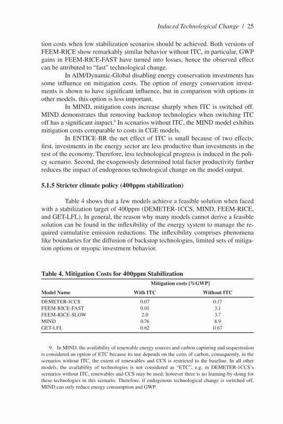
Table � shows that a few models achieve a feasible solution when faced with a stabilization target of �00ppm (DEMETER-1CCS, MInD, FEEM-RICE, and GET-�F�). In general, the reason why many models cannot derive a feasible solution can be found in the inflexibility of the energy system to manage the re-quired cumulative emission reductions. The inflexibility comprises phenomena like boundaries for the diffusion of backstop technologies, limited sets of mitiga-tion options or myopic investment behavior.
9. In MInD, the availability of renewable energy sources and carbon capturing and sequestration is considered an option of ETC because its use depends on the costs of carbon, consequently, in the scenarios without ITC, the extent of renewables and CCS is restricted to the baseline. In all other models, the availability of technologies is not considered as “ETC”, e.g. in DEMETER-1CCS�s scenarios without ITC, renewables and CCS may be used; however there is no learning-by-doing for these technologies in this scenario. Therefore, if endogenous technological change is switched off, MInD can only reduce energy consumption and GWP.
Induced Technological Change / 25
Table 4. Mitigation Costs for 400ppm Stabilization Mitigation costs [%GWP]
Model name With ITC Without ITC
DEMETER-1CCS 0.07 0.17 FEEM-RICE-FAST 0.01 3.1 FEEM-RICE-S�OW 2.0 3.7 MInD 0.76 �.9 GET-�F� 0.62 0.67
26 / The Energy Journal
5.1.6 Robust cost estimate
The IMCP set out not only to learn from the differences in model results, but also to identify robust findings. Is it possible to identify a robust estimate of climate protection costs across models in the IMCP?
One might be hesitant to see robustness in the broad range of costs e.g. in the case of �50ppm stabilization, ranging from benefits to costs greater than 6% of aggregate GWP 2000-2100 (at present value). However, the range is reduced con-siderably when we recognize that three models are of a predominantly exploratory nature, i.e. their intent is not to give a best estimate but to explore an extreme sce-nario. These are: IMAC�IM-R, which explores the role of the transportation sector under the assumption that energy sector and transportation sector are inflexible and externalities of investments in physical capital are biased against energy efficiency; AIM/Dynamic-Global limiting mitigation options to investments in energy conser-vation capital, hence emissions cannot be decoupled from economic growth in the long-run (these two models arrive at the highest costs in this study); FEEM-RICE-FAST exploring the possibility of “fast” technological change, which then results in benefits of climate protection rather than climate protection costs.
If we furthermore consider E3MG separately, because it is fundamentally different with its Keynesian rather than neoclassical point of view, we are thus left with a set of seven models and cost estimates that range from 0.0�% to 0.66% for �50ppm stabilization. Average climate protection costs among these remaining models are 0.39, 0.16, and 0.1%, for �50ppm, 500ppm, and 550ppm stabilization, respectively. Here, the MESSAGE-MACRO model is only included in the 500ppm average because it did not run the other scenarios. If we exclude the two energy system models that do not report costs in terms of GWP, the numbers only slightly change to 0.�1, 0.16, and 0.1 percent, for �50ppm, 500ppm, and 550ppm stabiliza-tion, respectively. These last numbers average over �, 5, and � models, respectively. Table 5 summarizes these values along with average costs at alternative discount rates, illustrating the influence of the discount rate on the cost estimate.
In view of this and with the considerable uncertainties about model structure and other assumptions in mind, it seems a robust conclusion from the presented energy system models and optimal growth models to expect climate protection costs of up to one percent.
5.2 Mitigation Strategies for different Stabilization Scenarios
In this section we identify the contributions of different carbon mitiga-tion options towards achieving an overall mitigation target, and we assess the role of technological change in the mitigation effort. Kaya�s identity10 provides a set of indicators that pinpoint the different ways taken by models to meet a given target,
10. Kaya�s identity originally also differentiates between income effect (GWP per capita) and a population effect. As an exogenous population scenario is used in this study, we can neglect this factor.
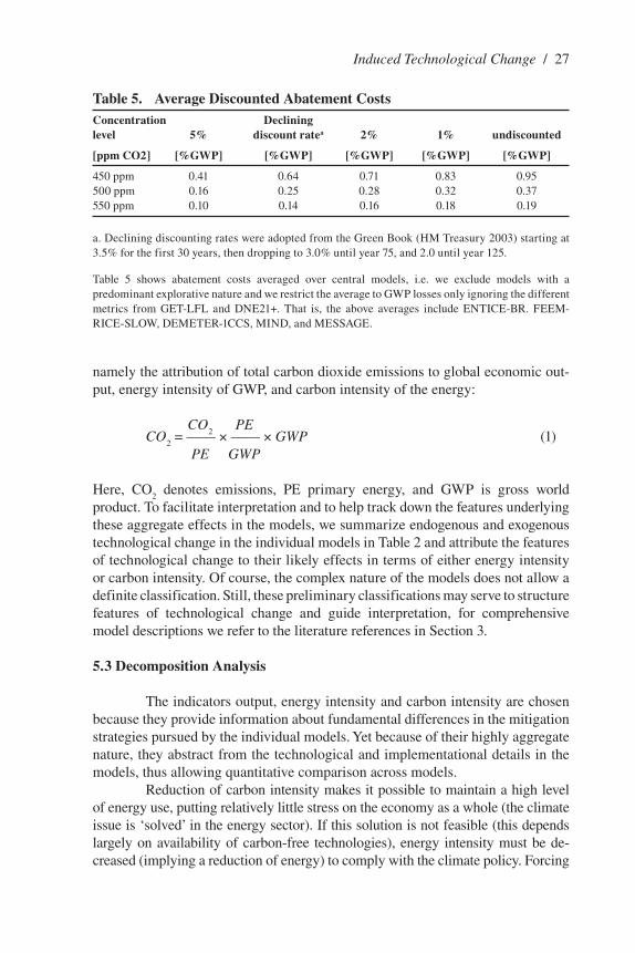
namely the attribution of total carbon dioxide emissions to global economic out-put, energy intensity of GWP, and carbon intensity of the energy:
CO2
PECO
2 = —— × —— × GWP (1)
PE GWP
Here, CO2 denotes emissions, PE primary energy, and GWP is gross world
product. To facilitate interpretation and to help track down the features underlying these aggregate effects in the models, we summarize endogenous and exogenous technological change in the individual models in Table 2 and attribute the features of technological change to their likely effects in terms of either energy intensity or carbon intensity. Of course, the complex nature of the models does not allow a definite classification. Still, these preliminary classifications may serve to structure features of technological change and guide interpretation, for comprehensive model descriptions we refer to the literature references in Section 3.
5.3 decomposition Analysis
The indicators output, energy intensity and carbon intensity are chosen because they provide information about fundamental differences in the mitigation strategies pursued by the individual models. Yet because of their highly aggregate nature, they abstract from the technological and implementational details in the models, thus allowing quantitative comparison across models.
Reduction of carbon intensity makes it possible to maintain a high level of energy use, putting relatively little stress on the economy as a whole (the climate issue is ‘solved� in the energy sector). If this solution is not feasible (this depends largely on availability of carbon-free technologies), energy intensity must be de-creased (implying a reduction of energy) to comply with the climate policy. Forcing
Induced Technological Change / 27
Table 5. Average discounted Abatement CostsConcentration declining level 5% discount ratea 2% 1% undiscounted
[ppm Co2] [%GWP] [%GWP] [%GWP] [%GWP] [%GWP]
�50 ppm 0.�1 0.6� 0.71 0.�3 0.95 500 ppm 0.16 0.25 0.2� 0.32 0.37 550 ppm 0.10 0.1� 0.16 0.1� 0.19
a. Declining discounting rates were adopted from the Green Book (HM Treasury 2003) starting at 3.5% for the first 30 years, then dropping to 3.0% until year 75, and 2.0 until year 125.
Table 5 shows abatement costs averaged over central models, i.e. we exclude models with a predominant explorative nature and we restrict the average to GWP losses only ignoring the different metrics from GET-�F� and DnE21+. That is, the above averages include EnTICE-BR. FEEM-RICE-S�OW, DEMETER-1CCS, MInD, and MESSAGE.
2� / The Energy Journal
the economy to use drastically less energy can amount to ‘choking� it, i.e. it may lead to a reduction in output (gross world product). The decomposition analysis allows quantification of the contribution of carbon intensity, energy intensity and output reduction to the required effort of emission reduction. For the purpose of this modeling comparison we use the refined �aspeyres index method (Sun 199�, Sun and Ang 2000). We apply the decomposition analysis to the differences of cumula-tive values between baseline and policy scenario. Figure 3 displays the decomposi-tion of the centennial CO
2 reductions along Kaya�s identity for different models.
5.3.1 Mitigation strategies to comply with 550ppm stabilization
The stacked bars in Figure 3 show the CO2 savings in the 550ppm policy
scenario from the baseline cumulated over the century. Additionally, shading indicate how much reductions in carbon intensity, energy intensity, and output (GWP) contribute to these savings.
The necessary carbon dioxide reductions differ widely between models. The cumulative reductions necessary to comply with a 550ppm concentration cap range from ~116GtC to ~9�7GtC (in FEEM-RICE and MInD, respectively), with correspondingly great differences in the challenge that these reduction pose for an economy.11 We stress that models tend to agree on the maximum cumulative CO
2 emissions for a given stabilization scenario: averages among models for
cumulative CO2 emissions are 5�9, 7�3, and 931 GtC for �50, 500, 550 ppm
stabilization scenarios, respectively. The corresponding standard deviations are 72, 77, and 92 GtC. The differences in Figure 3 stem mainly from different CO
2
emission paths in the baseline: cumulative CO2 emissions in the baseline range
from 9�0 to 2000 GtC, mean 1�30, with a standard deviation of 323 GtC. To account for such baseline effects, we will base our analyses on measures that are relative to this ‘mitigation effort� as much as possible.
note that baseline growth and CO2 emissions seem unrelated to model
types. This is not very surprising when growth and emissions are exogenous and therefore arbitrary. In other models, it is possible to calibrate growth and emissions, e.g. in recursive CGE models, by a variation of exogenous model parameters like the total factor productivity. In the optimal growth models, total factor productiv-ity, efficiency of R&D investments, and elasticity of substitution can be adjusted to approximate a given baseline scenario. However, the baseline is not determined by exogenous parameters alone but also by the endogenous features of technological change. This implies that CO
2 emissions of such models cannot be fully harmonized.
nevertheless, there is no reason to assume that models with endogenous technologi-cal change exhibit an inherent trend to particularly high or low emission scenarios.
A group of models (IMAC�IM-R and AIM/Dynamic-Global) share similar behavior. Here, the larger part of the CO
2 reductions can be attributed to
11. An obvious corollary is that emission reductions are necessary to meet even the 550ppm policy goal despite the presence of ETC in the baseline.
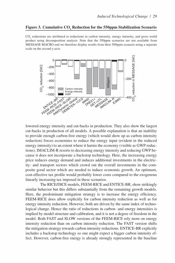
lowered energy intensity and cut-backs in production. They also show the largest cut-backs in production of all models. A possible explanation is that an inability to provide enough carbon-free energy (which would show up as carbon intensity reduction) forces economies to reduce the energy input (evident in the reduced energy intensity) to an extent where it harms the economy (visible as GWP reduc-tions). IMAC�IM-R resorts to decreasing energy intensity and reducing GWP be-cause it does not incorporate a backstop technology. Here, the increasing energy price reduces energy demand and induces additional investments in the electric-ity- and transport sectors which crowd out the overall investments in the com-posite good sector which are needed to induce economic growth. An optimum, cost-effective tax profile would probably lower costs compared to the exogenous linearly increasing tax imposed in these scenarios.
The RICE/DICE models, FEEM-RICE and EnTICE-BR, show strikingly similar behavior but this differs substantially from the remaining growth models. Here, the predominant mitigation strategy is to increase the energy efficiency. FEEM-RICE does allow explicitly for carbon intensity reduction as well as for energy intensity reduction. However, both are driven by the same index of techno-logical change. Hence the ratio of reductions in carbon- and energy intensities is implied by model structure and calibration, and it is not a degree of freedom in the model. Both FAST and S�OW versions of the FEEM-RICE rely more on energy intensity reduction than on carbon intensity reduction. The FAST version shifts the mitigation strategy towards carbon intensity reductions. EnTICE-BR explicitly includes a backstop technology so one might expect a bigger carbon intensity ef-fect. However, carbon-free energy is already strongly represented in the baseline
Induced Technological Change / 29
figure 3. Cumulative Co2 Reduction for the 550ppm Stabilization Scenario
CO2 reductions are attributed to reductions in carbon intensity, energy intensity, and gross world
product using decomposition analysis. note that the 550ppm scenarios are not available from MESSAGE-MACRO and we therefore display results from their 500ppm scenario using a separate scale on the second y-axis.
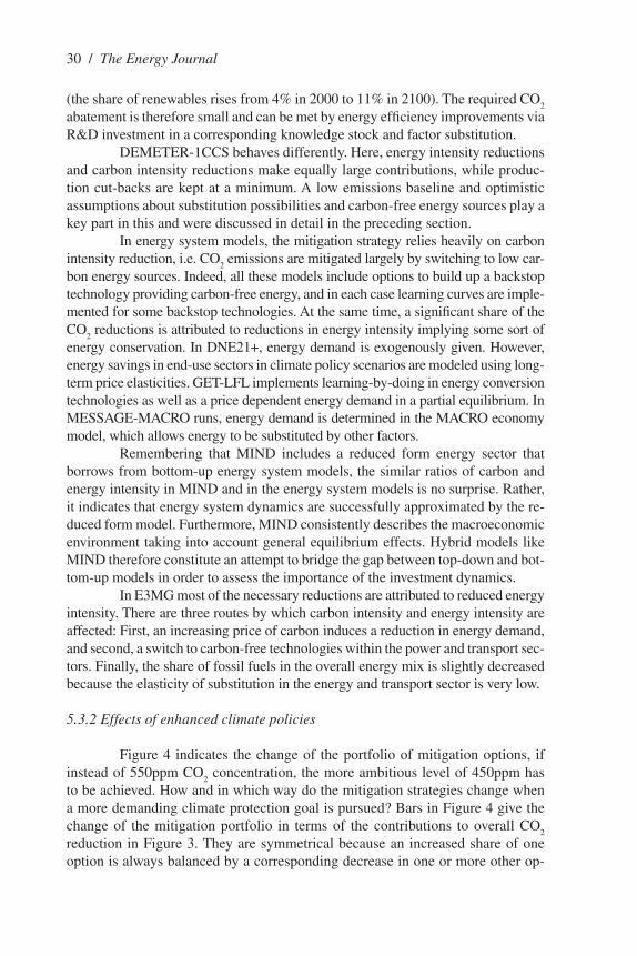
30 / The Energy Journal
(the share of renewables rises from �% in 2000 to 11% in 2100). The required CO2
abatement is therefore small and can be met by energy efficiency improvements via R&D investment in a corresponding knowledge stock and factor substitution.
DEMETER-1CCS behaves differently. Here, energy intensity reductions and carbon intensity reductions make equally large contributions, while produc-tion cut-backs are kept at a minimum. A low emissions baseline and optimistic assumptions about substitution possibilities and carbon-free energy sources play a key part in this and were discussed in detail in the preceding section.
In energy system models, the mitigation strategy relies heavily on carbon intensity reduction, i.e. CO
2 emissions are mitigated largely by switching to low car-
bon energy sources. Indeed, all these models include options to build up a backstop technology providing carbon-free energy, and in each case learning curves are imple-mented for some backstop technologies. At the same time, a significant share of the CO
2 reductions is attributed to reductions in energy intensity implying some sort of
energy conservation. In DnE21+, energy demand is exogenously given. However, energy savings in end-use sectors in climate policy scenarios are modeled using long-term price elasticities. GET-�F� implements learning-by-doing in energy conversion technologies as well as a price dependent energy demand in a partial equilibrium. In MESSAGE-MACRO runs, energy demand is determined in the MACRO economy model, which allows energy to be substituted by other factors.
Remembering that MInD includes a reduced form energy sector that borrows from bottom-up energy system models, the similar ratios of carbon and energy intensity in MInD and in the energy system models is no surprise. Rather, it indicates that energy system dynamics are successfully approximated by the re-duced form model. Furthermore, MInD consistently describes the macroeconomic environment taking into account general equilibrium effects. Hybrid models like MInD therefore constitute an attempt to bridge the gap between top-down and bot-tom-up models in order to assess the importance of the investment dynamics.
In E3MG most of the necessary reductions are attributed to reduced energy intensity. There are three routes by which carbon intensity and energy intensity are affected: First, an increasing price of carbon induces a reduction in energy demand, and second, a switch to carbon-free technologies within the power and transport sec-tors. Finally, the share of fossil fuels in the overall energy mix is slightly decreased because the elasticity of substitution in the energy and transport sector is very low.
5.3.2 Effects of enhanced climate policies
Figure � indicates the change of the portfolio of mitigation options, if instead of 550ppm CO
2 concentration, the more ambitious level of �50ppm has
to be achieved. How and in which way do the mitigation strategies change when a more demanding climate protection goal is pursued? Bars in Figure � give the change of the mitigation portfolio in terms of the contributions to overall CO
2
reduction in Figure 3. They are symmetrical because an increased share of one option is always balanced by a corresponding decrease in one or more other op-
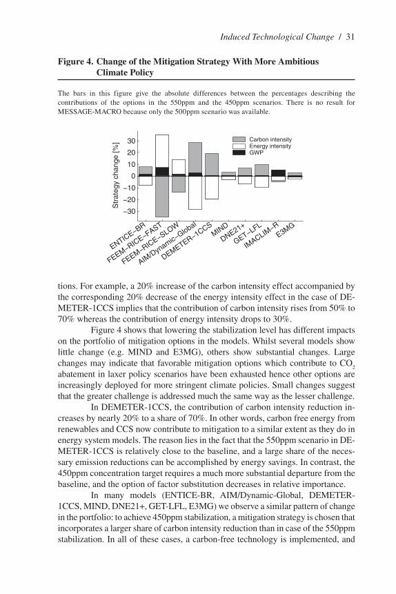
tions. For example, a 20% increase of the carbon intensity effect accompanied by the corresponding 20% decrease of the energy intensity effect in the case of DE-METER-1CCS implies that the contribution of carbon intensity rises from 50% to 70% whereas the contribution of energy intensity drops to 30%.
Figure � shows that lowering the stabilization level has different impacts on the portfolio of mitigation options in the models. Whilst several models show little change (e.g. MInD and E3MG), others show substantial changes. �arge changes may indicate that favorable mitigation options which contribute to CO
2
abatement in laxer policy scenarios have been exhausted hence other options are increasingly deployed for more stringent climate policies. Small changes suggest that the greater challenge is addressed much the same way as the lesser challenge.
In DEMETER-1CCS, the contribution of carbon intensity reduction in-creases by nearly 20% to a share of 70%. In other words, carbon free energy from renewables and CCS now contribute to mitigation to a similar extent as they do in energy system models. The reason lies in the fact that the 550ppm scenario in DE-METER-1CCS is relatively close to the baseline, and a large share of the neces-sary emission reductions can be accomplished by energy savings. In contrast, the �50ppm concentration target requires a much more substantial departure from the baseline, and the option of factor substitution decreases in relative importance.
In many models (EnTICE-BR, AIM/Dynamic-Global, DEMETER-1CCS, MInD, DnE21+, GET-�F�, E3MG) we observe a similar pattern of change in the portfolio: to achieve �50ppm stabilization, a mitigation strategy is chosen that incorporates a larger share of carbon intensity reduction than in case of the 550ppm stabilization. In all of these cases, a carbon-free technology is implemented, and
Induced Technological Change / 31
figure 4. Change of the Mitigation Strategy With More Ambitious Climate Policy
The bars in this figure give the absolute differences between the percentages describing the contributions of the options in the 550ppm and the �50ppm scenarios. There is no result for MESSAGE-MACRO because only the 500ppm scenario was available.
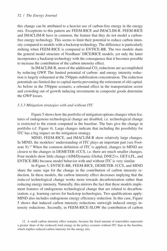
32 / The Energy Journal
this change can be attributed to a heavier use of carbon-free energy in the energy mix. Exceptions to this pattern are FEEM-RICE and IMAC�IM-R. FEEM-RICE and IMAC�IM-R have in common, the feature that they do not model a carbon-free energy technology. This seems to limit their potential to reduce carbon inten-sity compared to models with a backstop technology. The difference is particularly striking when FEEM-RICE is compared to EnTICE-BR. The two models share the general model structure of nordhaus� DICE/RICE models, yet only the latter incorporates a backstop technology with the consequence that it becomes possible to increase the contribution of the carbon intensity effect.
In IMAC�IM-R, most of the additional CO2 reductions are accomplished
by reducing GWP. The limited potential of carbon- and energy intensity reduc-tion is largely exhausted at the 550ppm stabilization concentration. The reduction potentials are limited due to capital inertia preventing the retirement of old capital. As before in the 550ppm scenario, a rebound effect in the transportation sector and crowding out of growth inducing investments in composite goods determine the GWP losses.
5.3.3 Mitigation strategies with and without ITC
Figure 5 shows how the portfolio of mitigation options changes when fea-tures of endogenous technological change are disabled, i.e. technological change is restricted to the extent computed in the baseline. The bars give the change in portfolio (cf. Figure �). �arge changes indicate that including the possibility for ITC has a big impact on the mitigation strategy.
MInD, FEEM-RICE, and IMAC�IM-R show relatively large changes. In MInD, the modelers� understanding of ITC plays an important part (see Foot-note 9).12 When the common definition of ITC is applied, changes in MInD are closest to the changes in DEMETER-1CCS, i.e. there are much smaller changes. Four models show little change (AIM/Dynamic-Global, DnE21+, GET-�F�, and EnTICE-BR) because model behavior with and without ITC is very similar.
In Figure 5, EnTICE-BR, FEEM-RICE, DEMETER-1CCS, and MInD share the same sign for the change in the contribution of carbon intensity re-duction. In these models, the carbon intensity effect decreases implying that the induced technological change works more towards decarbonization rather than reducing energy intensity. naturally, this mirrors the fact that these models imple-ment features of endogenous technological change that are related to decarbon-ization, e.g. learning curves for backstop technologies. Two qualifications apply: MInD also includes endogenous energy efficiency reduction. In this case, Figure 5 shows that induced carbon intensity reductions outweigh induced energy in-tensity reductions. Secondly, in FEEM-RICE-S�OW the contribution of carbon
12. A small carbon intensity effect remains, because the fixed amount of renewables represents a greater share of the (reduced) total energy in the policy scenario without ITC than in the baseline, which implies reduced carbon intensity for the energy mix.
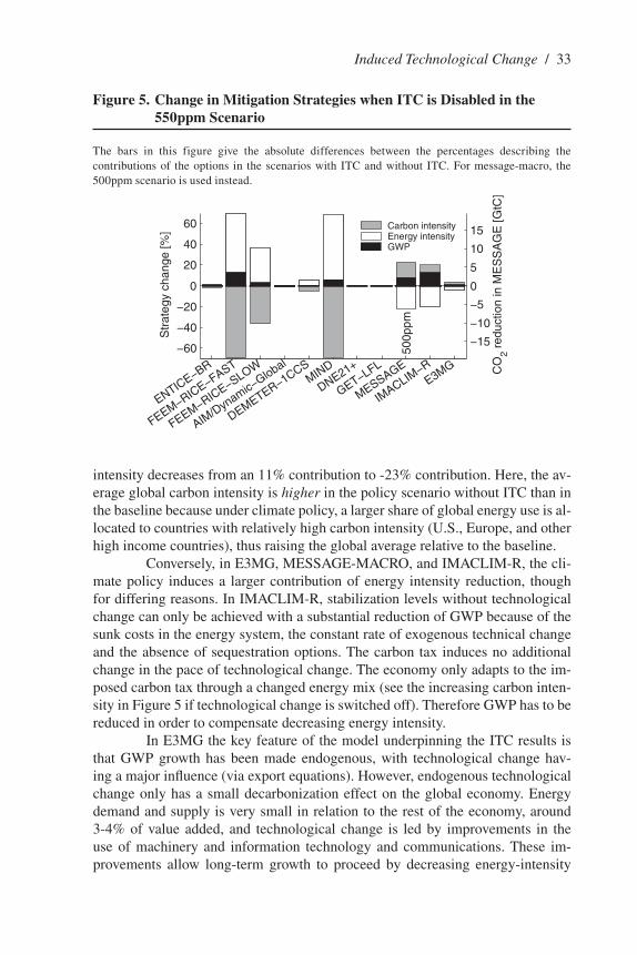
intensity decreases from an 11% contribution to -23% contribution. Here, the av-erage global carbon intensity is higher in the policy scenario without ITC than in the baseline because under climate policy, a larger share of global energy use is al-located to countries with relatively high carbon intensity (U.S., Europe, and other high income countries), thus raising the global average relative to the baseline.
Conversely, in E3MG, MESSAGE-MACRO, and IMAC�IM-R, the cli-mate policy induces a larger contribution of energy intensity reduction, though for differing reasons. In IMAC�IM-R, stabilization levels without technological change can only be achieved with a substantial reduction of GWP because of the sunk costs in the energy system, the constant rate of exogenous technical change and the absence of sequestration options. The carbon tax induces no additional change in the pace of technological change. The economy only adapts to the im-posed carbon tax through a changed energy mix (see the increasing carbon inten-sity in Figure 5 if technological change is switched off). Therefore GWP has to be reduced in order to compensate decreasing energy intensity.
In E3MG the key feature of the model underpinning the ITC results is that GWP growth has been made endogenous, with technological change hav-ing a major influence (via export equations). However, endogenous technological change only has a small decarbonization effect on the global economy. Energy demand and supply is very small in relation to the rest of the economy, around 3-�% of value added, and technological change is led by improvements in the use of machinery and information technology and communications. These im-provements allow long-term growth to proceed by decreasing energy-intensity
Induced Technological Change / 33
figure 5. Change in Mitigation Strategies when ITC is disabled in the 550ppm Scenario
The bars in this figure give the absolute differences between the percentages describing the contributions of the options in the scenarios with ITC and without ITC. For message-macro, the 500ppm scenario is used instead.
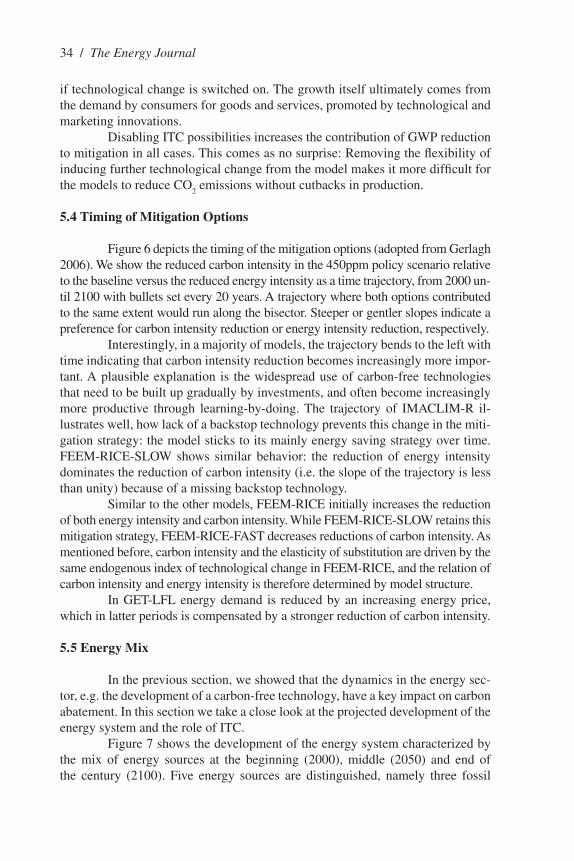
3� / The Energy Journal
if technological change is switched on. The growth itself ultimately comes from the demand by consumers for goods and services, promoted by technological and marketing innovations.
Disabling ITC possibilities increases the contribution of GWP reduction to mitigation in all cases. This comes as no surprise: Removing the flexibility of inducing further technological change from the model makes it more difficult for the models to reduce CO
2 emissions without cutbacks in production.
5.4 Timing of Mitigation options
Figure 6 depicts the timing of the mitigation options (adopted from Gerlagh 2006). We show the reduced carbon intensity in the �50ppm policy scenario relative to the baseline versus the reduced energy intensity as a time trajectory, from 2000 un-til 2100 with bullets set every 20 years. A trajectory where both options contributed to the same extent would run along the bisector. Steeper or gentler slopes indicate a preference for carbon intensity reduction or energy intensity reduction, respectively.
Interestingly, in a majority of models, the trajectory bends to the left with time indicating that carbon intensity reduction becomes increasingly more impor-tant. A plausible explanation is the widespread use of carbon-free technologies that need to be built up gradually by investments, and often become increasingly more productive through learning-by-doing. The trajectory of IMAC�IM-R il-lustrates well, how lack of a backstop technology prevents this change in the miti-gation strategy: the model sticks to its mainly energy saving strategy over time. FEEM-RICE-S�OW shows similar behavior: the reduction of energy intensity dominates the reduction of carbon intensity (i.e. the slope of the trajectory is less than unity) because of a missing backstop technology.
Similar to the other models, FEEM-RICE initially increases the reduction of both energy intensity and carbon intensity. While FEEM-RICE-S�OW retains this mitigation strategy, FEEM-RICE-FAST decreases reductions of carbon intensity. As mentioned before, carbon intensity and the elasticity of substitution are driven by the same endogenous index of technological change in FEEM-RICE, and the relation of carbon intensity and energy intensity is therefore determined by model structure.
In GET-�F� energy demand is reduced by an increasing energy price, which in latter periods is compensated by a stronger reduction of carbon intensity.
5.5 Energy Mix
In the previous section, we showed that the dynamics in the energy sec-tor, e.g. the development of a carbon-free technology, have a key impact on carbon abatement. In this section we take a close look at the projected development of the energy system and the role of ITC.
Figure 7 shows the development of the energy system characterized by the mix of energy sources at the beginning (2000), middle (2050) and end of the century (2100). Five energy sources are distinguished, namely three fossil
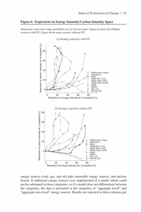
energy sources (coal, gas, and oil) plus renewable energy sources, and nuclear fission. If additional energy sources were implemented in a model which could not be subsumed in these categories, or if a model does not differentiate between the categories, the data is presented in the categories of “aggregate fossil” and “aggregate non-fossil” energy sources. Results are reported in three columns per
Induced Technological Change / 35
figure 6. Trajectories in Energy Intensity/Carbon Intensity Space
Trajectories start at the origin and bullets are set 20 years apart. Figure 6a shows the �50ppm scenario with ITC, Figure 6b the same scenario without ITC.
(a) Strategy trajectory with ITC
(b) Strategy trajectory without ITC
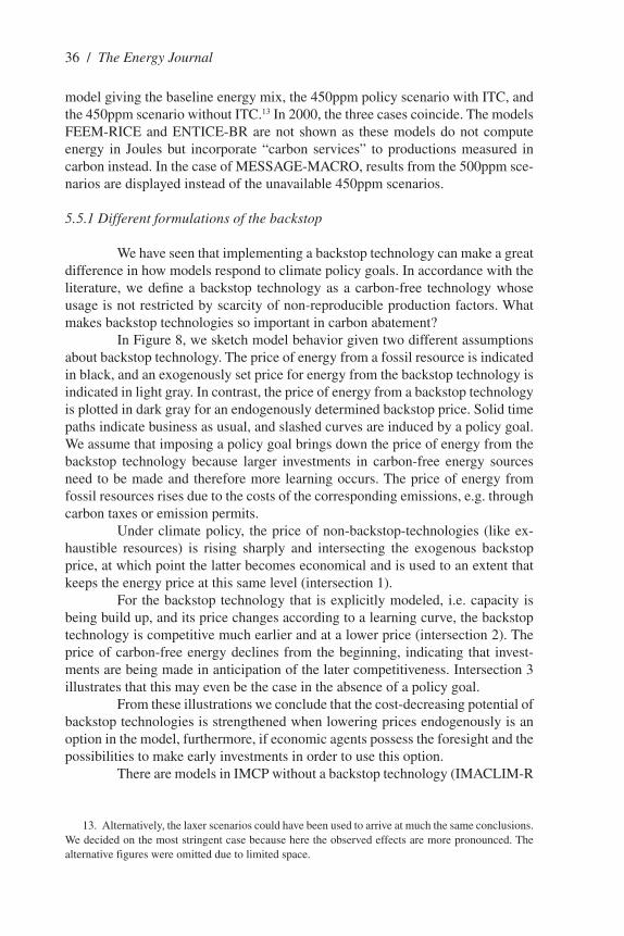
36 / The Energy Journal
model giving the baseline energy mix, the �50ppm policy scenario with ITC, and the �50ppm scenario without ITC.13 In 2000, the three cases coincide. The models FEEM-RICE and EnTICE-BR are not shown as these models do not compute energy in Joules but incorporate “carbon services” to productions measured in carbon instead. In the case of MESSAGE-MACRO, results from the 500ppm sce-narios are displayed instead of the unavailable �50ppm scenarios.
5.5.1 Different formulations of the backstop
We have seen that implementing a backstop technology can make a great difference in how models respond to climate policy goals. In accordance with the literature, we define a backstop technology as a carbon-free technology whose usage is not restricted by scarcity of non-reproducible production factors. What makes backstop technologies so important in carbon abatement?
In Figure �, we sketch model behavior given two different assumptions about backstop technology. The price of energy from a fossil resource is indicated in black, and an exogenously set price for energy from the backstop technology is indicated in light gray. In contrast, the price of energy from a backstop technology is plotted in dark gray for an endogenously determined backstop price. Solid time paths indicate business as usual, and slashed curves are induced by a policy goal. We assume that imposing a policy goal brings down the price of energy from the backstop technology because larger investments in carbon-free energy sources need to be made and therefore more learning occurs. The price of energy from fossil resources rises due to the costs of the corresponding emissions, e.g. through carbon taxes or emission permits.
Under climate policy, the price of non-backstop-technologies (like ex-haustible resources) is rising sharply and intersecting the exogenous backstop price, at which point the latter becomes economical and is used to an extent that keeps the energy price at this same level (intersection 1).
For the backstop technology that is explicitly modeled, i.e. capacity is being build up, and its price changes according to a learning curve, the backstop technology is competitive much earlier and at a lower price (intersection 2). The price of carbon-free energy declines from the beginning, indicating that invest-ments are being made in anticipation of the later competitiveness. Intersection 3 illustrates that this may even be the case in the absence of a policy goal.
From these illustrations we conclude that the cost-decreasing potential of backstop technologies is strengthened when lowering prices endogenously is an option in the model, furthermore, if economic agents possess the foresight and the possibilities to make early investments in order to use this option.
There are models in IMCP without a backstop technology (IMAC�IM-R
13. Alternatively, the laxer scenarios could have been used to arrive at much the same conclusions. We decided on the most stringent case because here the observed effects are more pronounced. The alternative figures were omitted due to limited space.
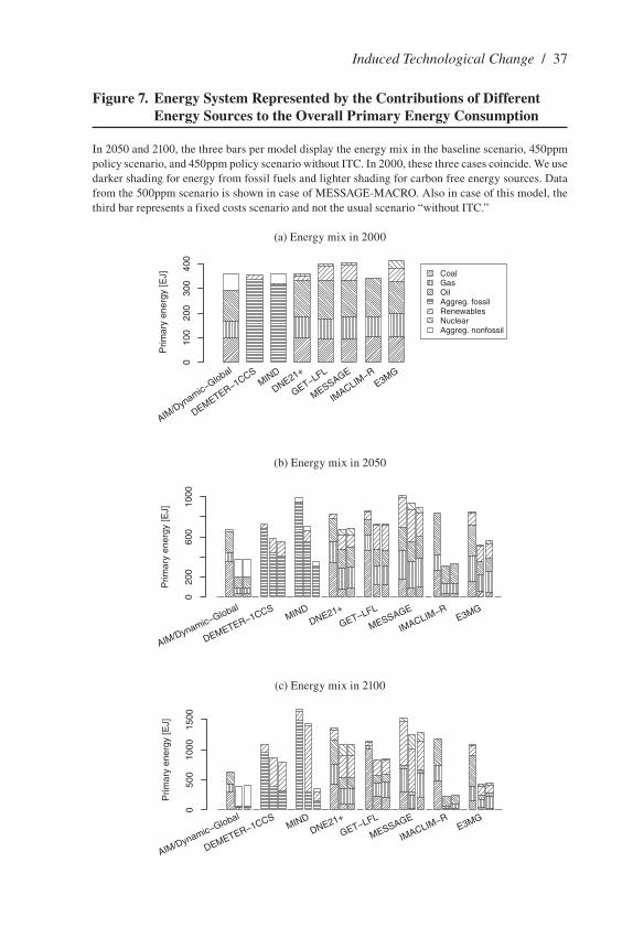
Induced Technological Change / 37
figure 7. Energy System Represented by the Contributions of different Energy Sources to the overall Primary Energy Consumption
In 2050 and 2100, the three bars per model display the energy mix in the baseline scenario, �50ppm policy scenario, and �50ppm policy scenario without ITC. In 2000, these three cases coincide. We use darker shading for energy from fossil fuels and lighter shading for carbon free energy sources. Data from the 500ppm scenario is shown in case of MESSAGE-MACRO. Also in case of this model, the third bar represents a fixed costs scenario and not the usual scenario “without ITC.”
(a) Energy mix in 2000
(b) Energy mix in 2050
(c) Energy mix in 2100
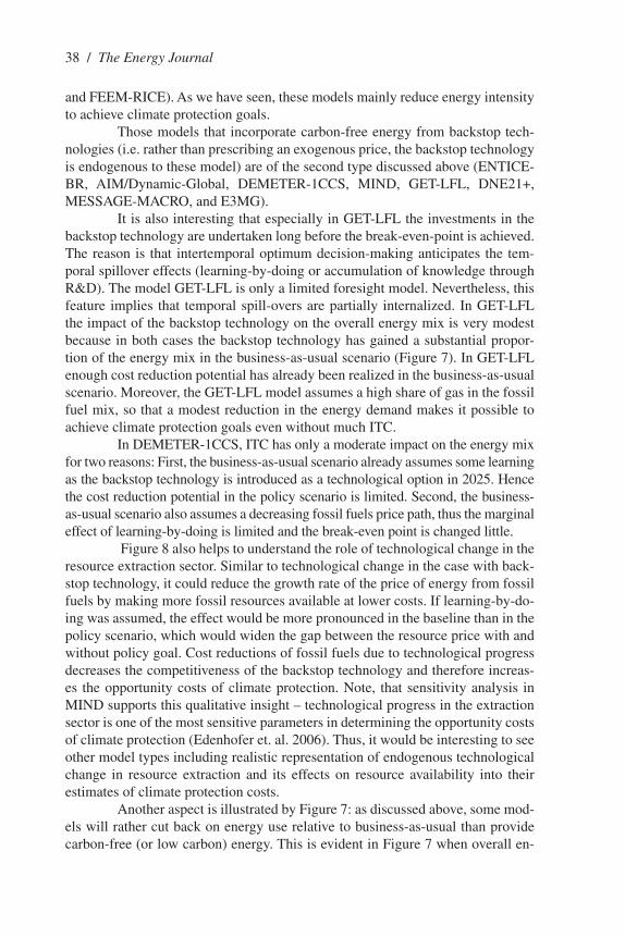
3� / The Energy Journal
and FEEM-RICE). As we have seen, these models mainly reduce energy intensity to achieve climate protection goals.
Those models that incorporate carbon-free energy from backstop tech-nologies (i.e. rather than prescribing an exogenous price, the backstop technology is endogenous to these model) are of the second type discussed above (EnTICE-BR, AIM/Dynamic-Global, DEMETER-1CCS, MInD, GET-�F�, DnE21+, MESSAGE-MACRO, and E3MG).
It is also interesting that especially in GET-�F� the investments in the backstop technology are undertaken long before the break-even-point is achieved. The reason is that intertemporal optimum decision-making anticipates the tem-poral spillover effects (learning-by-doing or accumulation of knowledge through R&D). The model GET-�F� is only a limited foresight model. nevertheless, this feature implies that temporal spill-overs are partially internalized. In GET-�F� the impact of the backstop technology on the overall energy mix is very modest because in both cases the backstop technology has gained a substantial propor-tion of the energy mix in the business-as-usual scenario (Figure 7). In GET-�F� enough cost reduction potential has already been realized in the business-as-usual scenario. Moreover, the GET-�F� model assumes a high share of gas in the fossil fuel mix, so that a modest reduction in the energy demand makes it possible to achieve climate protection goals even without much ITC.
In DEMETER-1CCS, ITC has only a moderate impact on the energy mix for two reasons: First, the business-as-usual scenario already assumes some learning as the backstop technology is introduced as a technological option in 2025. Hence the cost reduction potential in the policy scenario is limited. Second, the business-as-usual scenario also assumes a decreasing fossil fuels price path, thus the marginal effect of learning-by-doing is limited and the break-even point is changed little.
Figure � also helps to understand the role of technological change in the resource extraction sector. Similar to technological change in the case with back-stop technology, it could reduce the growth rate of the price of energy from fossil fuels by making more fossil resources available at lower costs. If learning-by-do-ing was assumed, the effect would be more pronounced in the baseline than in the policy scenario, which would widen the gap between the resource price with and without policy goal. Cost reductions of fossil fuels due to technological progress decreases the competitiveness of the backstop technology and therefore increas-es the opportunity costs of climate protection. note, that sensitivity analysis in MInD supports this qualitative insight – technological progress in the extraction sector is one of the most sensitive parameters in determining the opportunity costs of climate protection (Edenhofer et. al. 2006). Thus, it would be interesting to see other model types including realistic representation of endogenous technological change in resource extraction and its effects on resource availability into their estimates of climate protection costs.
Another aspect is illustrated by Figure 7: as discussed above, some mod-els will rather cut back on energy use relative to business-as-usual than provide carbon-free (or low carbon) energy. This is evident in Figure 7 when overall en-
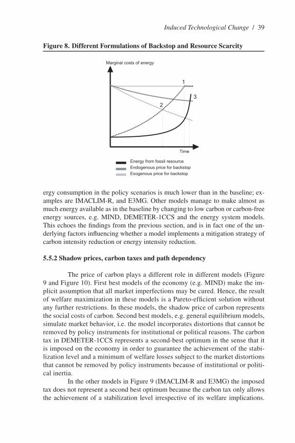
ergy consumption in the policy scenarios is much lower than in the baseline; ex-amples are IMAC�IM-R, and E3MG. Other models manage to make almost as much energy available as in the baseline by changing to low carbon or carbon-free energy sources, e.g. MInD, DEMETER-1CCS and the energy system models. This echoes the findings from the previous section, and is in fact one of the un-derlying factors influencing whether a model implements a mitigation strategy of carbon intensity reduction or energy intensity reduction.
5.5.2 Shadow prices, carbon taxes and path dependency
The price of carbon plays a different role in different models (Figure 9 and Figure 10). First best models of the economy (e.g. MInD) make the im-plicit assumption that all market imperfections may be cured. Hence, the result of welfare maximization in these models is a Pareto-efficient solution without any further restrictions. In these models, the shadow price of carbon represents the social costs of carbon. Second best models, e.g. general equilibrium models, simulate market behavior, i.e. the model incorporates distortions that cannot be removed by policy instruments for institutional or political reasons. The carbon tax in DEMETER-1CCS represents a second-best optimum in the sense that it is imposed on the economy in order to guarantee the achievement of the stabi-lization level and a minimum of welfare losses subject to the market distortions that cannot be removed by policy instruments because of institutional or politi-cal inertia.
In the other models in Figure 9 (IMAC�IM-R and E3MG) the imposed tax does not represent a second best optimum because the carbon tax only allows the achievement of a stabilization level irrespective of its welfare implications.
Induced Technological Change / 39
figure 8. different formulations of Backstop and Resource Scarcity
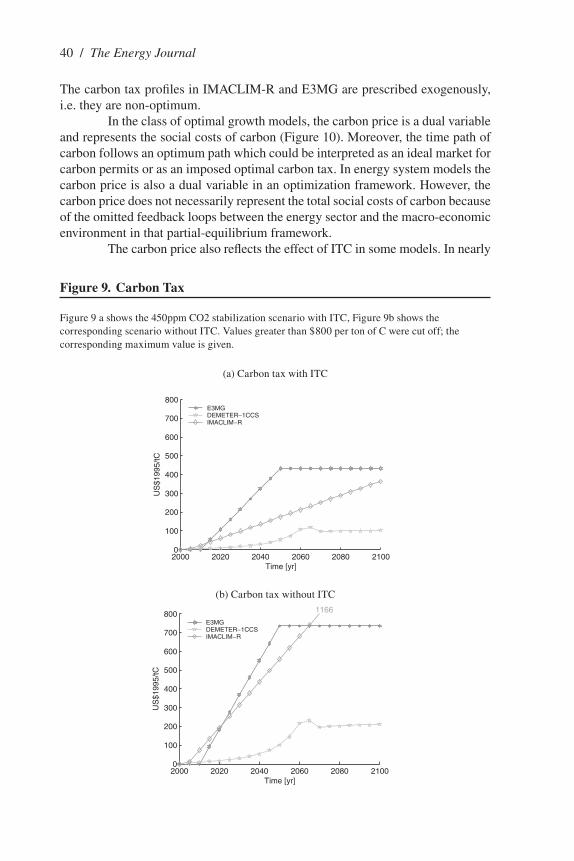
�0 / The Energy Journal
The carbon tax profiles in IMAC�IM-R and E3MG are prescribed exogenously, i.e. they are non-optimum.
In the class of optimal growth models, the carbon price is a dual variable and represents the social costs of carbon (Figure 10). Moreover, the time path of carbon follows an optimum path which could be interpreted as an ideal market for carbon permits or as an imposed optimal carbon tax. In energy system models the carbon price is also a dual variable in an optimization framework. However, the carbon price does not necessarily represent the total social costs of carbon because of the omitted feedback loops between the energy sector and the macro-economic environment in that partial-equilibrium framework.
The carbon price also reflects the effect of ITC in some models. In nearly
figure 9. Carbon Tax
Figure 9 a shows the �50ppm CO2 stabilization scenario with ITC, Figure 9b shows the corresponding scenario without ITC. Values greater than $�00 per ton of C were cut off; the corresponding maximum value is given.
(a) Carbon tax with ITC
(b) Carbon tax without ITC
Induced Technological Change / �1
all models the carbon price is higher in the scenarios without technological change. However, in MInD the carbon price behaves differently: it increases exponentially in the case without ITC but it peaks and decreases if ITC is switched on.
There is an interesting pattern in carbon price development in some mod-els: towards the end of the century, the shadow price reaches a maximum and be-gins to decline. This is true for all scenarios with ITC in MInD and in the �50ppm scenario for DEMETER-1CCS. If the price of the backstop technology decreases over time, even without an increasing shadow price of emissions (and fossil fuel price), the backstop technology remains competitive with fossil fuels. In contrast to a model with an exogenous price of the backstop technology, learning-by-do-ing of the backstop technology creates a path dependency because its price is determined endogenously by investments in learning-by-doing. There is no longer an incentive for investors to promote fossil fuels after the energy system is trans-formed because the price of the backstop technology also declines with the trans-formation of the energy system. The shadow price in most energy system models increases throughout the century indicating that the transformation of the energy system is not completed before 2100. This may be in part because renewables or nuclear power (as backstop technologies) are not able to substitute fossil fuels un-til the end of the century, due to bounds on market share for renewables, moderate price increases for fossil fuels that remain too low to trigger a transformation, and relatively optimistic assumptions about CCS. The remaining share of fossil fuels will turn carbon into a scarce factor in production with a positive price.
Path dependencies occur if the transformation to a carbon-free energy system is irreversible in that the carbon-free technologies become the least cost set of options.
5.5.3 The specific role of carbon capturing and sequestration
Among the participating models, five explicitly incorporate the option of capturing and storing CO
2 emissions from combustion (DEMETER-1CCS,
MInD, DnE21+, GET-�F�, and MESSAGE-MACRO). Figure 11 shows how much CO
2 is captured in different scenarios, accumulated over the century. Fig-
ure 12 gives the corresponding time paths of carbon capturing and sequestration (CCS) for one exemplary scenario (500ppm CO
2 stabilization).
As one would expect, Figure 11 shows that the more challenging the climate policy target, the more CO
2 is captured and stored. There is no CCS in the
baseline, as capture and storage of CO2 is costly and hence only becomes econom-
ical in the presence of climate policy. DnE21+ is an exception, because the model includes an option to use CCS in the context of enhanced oil recovery which makes CCS economical in its own right. The contribution to overall abatement (the difference of cumulative emissions between baseline and policy scenarios) is substantial, in particular in MInD, DnE21+, and GET-�F�. However, nowhere is CCS the dominant mitigation option but rather, it is always predicted to be one
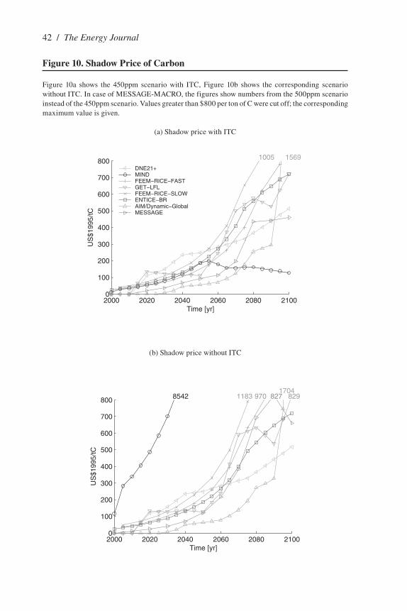
�2 / The Energy Journal
figure 10. Shadow Price of Carbon
Figure 10a shows the �50ppm scenario with ITC, Figure 10b shows the corresponding scenario without ITC. In case of MESSAGE-MACRO, the figures show numbers from the 500ppm scenario instead of the �50ppm scenario. Values greater than $�00 per ton of C were cut off; the corresponding maximum value is given.
(a) Shadow price with ITC
(b) Shadow price without ITC
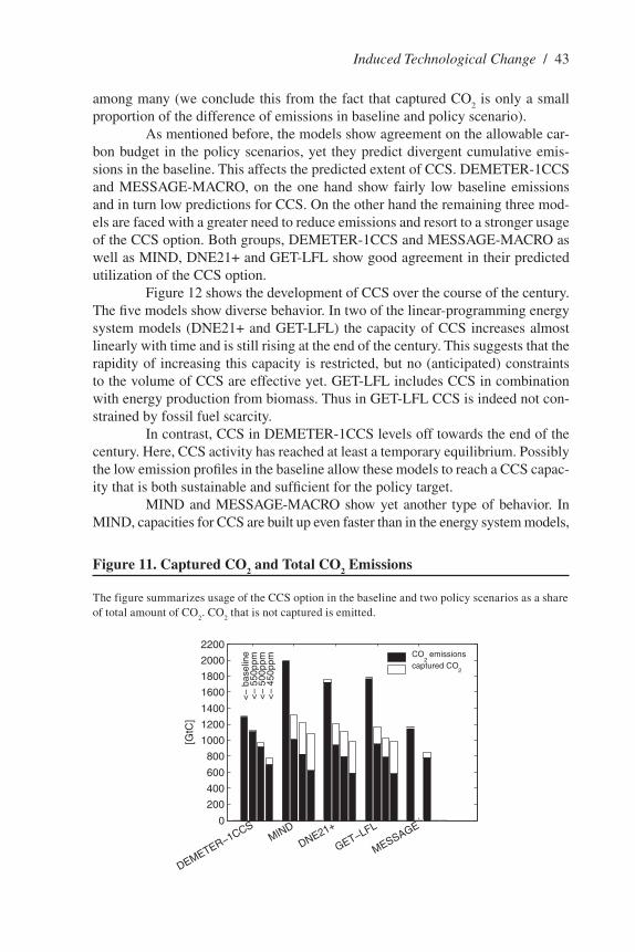
among many (we conclude this from the fact that captured CO2 is only a small
proportion of the difference of emissions in baseline and policy scenario).As mentioned before, the models show agreement on the allowable car-
bon budget in the policy scenarios, yet they predict divergent cumulative emis-sions in the baseline. This affects the predicted extent of CCS. DEMETER-1CCS and MESSAGE-MACRO, on the one hand show fairly low baseline emissions and in turn low predictions for CCS. On the other hand the remaining three mod-els are faced with a greater need to reduce emissions and resort to a stronger usage of the CCS option. Both groups, DEMETER-1CCS and MESSAGE-MACRO as well as MInD, DnE21+ and GET-�F� show good agreement in their predicted utilization of the CCS option.
Figure 12 shows the development of CCS over the course of the century. The five models show diverse behavior. In two of the linear-programming energy system models (DnE21+ and GET-�F�) the capacity of CCS increases almost linearly with time and is still rising at the end of the century. This suggests that the rapidity of increasing this capacity is restricted, but no (anticipated) constraints to the volume of CCS are effective yet. GET-�F� includes CCS in combination with energy production from biomass. Thus in GET-�F� CCS is indeed not con-strained by fossil fuel scarcity.
In contrast, CCS in DEMETER-1CCS levels off towards the end of the century. Here, CCS activity has reached at least a temporary equilibrium. Possibly the low emission profiles in the baseline allow these models to reach a CCS capac-ity that is both sustainable and sufficient for the policy target.
MInD and MESSAGE-MACRO show yet another type of behavior. In MInD, capacities for CCS are built up even faster than in the energy system models,
Induced Technological Change / �3
figure 11. Captured Co2 and Total Co2 Emissions
The figure summarizes usage of the CCS option in the baseline and two policy scenarios as a share of total amount of CO
2. CO
2 that is not captured is emitted.
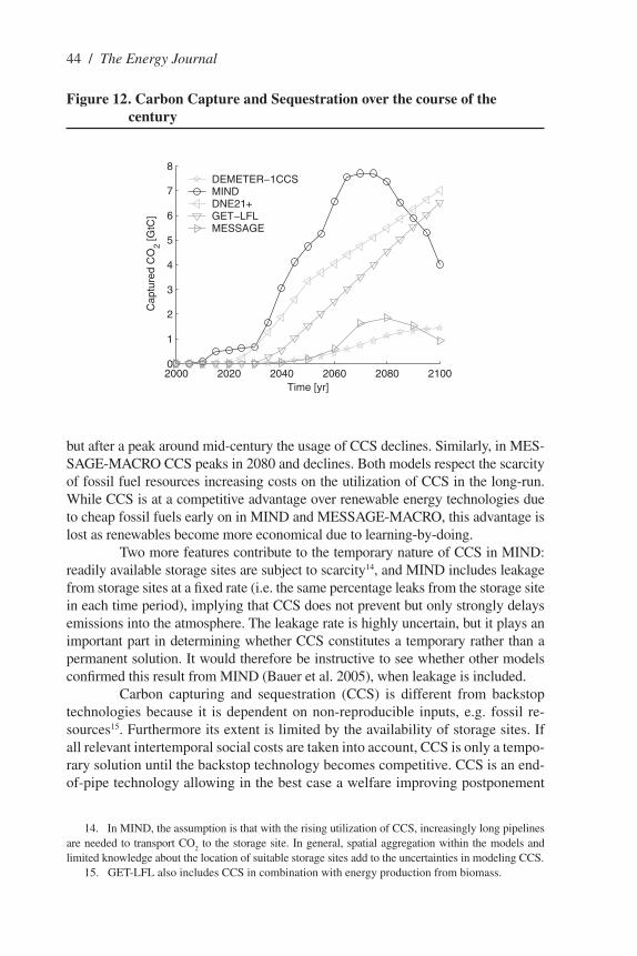
�� / The Energy Journal
but after a peak around mid-century the usage of CCS declines. Similarly, in MES-SAGE-MACRO CCS peaks in 20�0 and declines. Both models respect the scarcity of fossil fuel resources increasing costs on the utilization of CCS in the long-run. While CCS is at a competitive advantage over renewable energy technologies due to cheap fossil fuels early on in MInD and MESSAGE-MACRO, this advantage is lost as renewables become more economical due to learning-by-doing.
Two more features contribute to the temporary nature of CCS in MInD: readily available storage sites are subject to scarcity1�, and MInD includes leakage from storage sites at a fixed rate (i.e. the same percentage leaks from the storage site in each time period), implying that CCS does not prevent but only strongly delays emissions into the atmosphere. The leakage rate is highly uncertain, but it plays an important part in determining whether CCS constitutes a temporary rather than a permanent solution. It would therefore be instructive to see whether other models confirmed this result from MInD (Bauer et al. 2005), when leakage is included.
Carbon capturing and sequestration (CCS) is different from backstop technologies because it is dependent on non-reproducible inputs, e.g. fossil re-sources15. Furthermore its extent is limited by the availability of storage sites. If all relevant intertemporal social costs are taken into account, CCS is only a tempo-rary solution until the backstop technology becomes competitive. CCS is an end-of-pipe technology allowing in the best case a welfare improving postponement
1�. In MInD, the assumption is that with the rising utilization of CCS, increasingly long pipelines are needed to transport CO
2 to the storage site. In general, spatial aggregation within the models and
limited knowledge about the location of suitable storage sites add to the uncertainties in modeling CCS.15. GET-�F� also includes CCS in combination with energy production from biomass.
figure 12. Carbon Capture and Sequestration over the course of the century
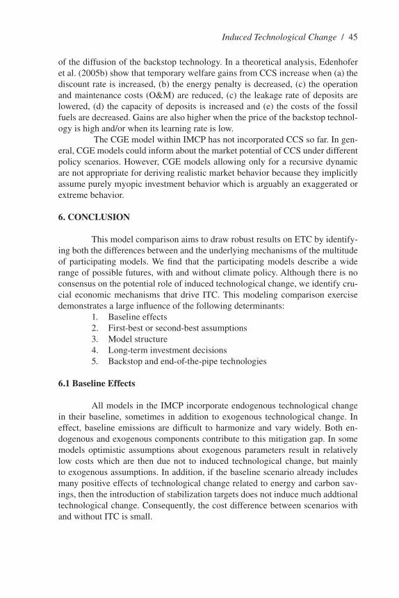
of the diffusion of the backstop technology. In a theoretical analysis, Edenhofer et al. (2005b) show that temporary welfare gains from CCS increase when (a) the discount rate is increased, (b) the energy penalty is decreased, (c) the operation and maintenance costs (O&M) are reduced, (c) the leakage rate of deposits are lowered, (d) the capacity of deposits is increased and (e) the costs of the fossil fuels are decreased. Gains are also higher when the price of the backstop technol-ogy is high and/or when its learning rate is low.
The CGE model within IMCP has not incorporated CCS so far. In gen-eral, CGE models could inform about the market potential of CCS under different policy scenarios. However, CGE models allowing only for a recursive dynamic are not appropriate for deriving realistic market behavior because they implicitly assume purely myopic investment behavior which is arguably an exaggerated or extreme behavior.
6. ConCluSIon
This model comparison aims to draw robust results on ETC by identify-ing both the differences between and the underlying mechanisms of the multitude of participating models. We find that the participating models describe a wide range of possible futures, with and without climate policy. Although there is no consensus on the potential role of induced technological change, we identify cru-cial economic mechanisms that drive ITC. This modeling comparison exercise demonstrates a large influence of the following determinants:
1. Baseline effects2. First-best or second-best assumptions3. Model structure�. �ong-term investment decisions5. Backstop and end-of-the-pipe technologies
6.1 Baseline Effects
All models in the IMCP incorporate endogenous technological change in their baseline, sometimes in addition to exogenous technological change. In effect, baseline emissions are difficult to harmonize and vary widely. Both en-dogenous and exogenous components contribute to this mitigation gap. In some models optimistic assumptions about exogenous parameters result in relatively low costs which are then due not to induced technological change, but mainly to exogenous assumptions. In addition, if the baseline scenario already includes many positive effects of technological change related to energy and carbon sav-ings, then the introduction of stabilization targets does not induce much addtional technological change. Consequently, the cost difference between scenarios with and without ITC is small.
Induced Technological Change / �5
�6 / The Energy Journal
6.2 first Best or Second Best Assumptions
It has important consequences whether a first best or a second best world is modeled: First best models implicitly assume perfect markets and the imple-mentation of optimum policy tools. In other words, first best models preclude so called no-regret options. Therefore, they are inherently more pessimistic about the costs of climate protection because climate protection reallocates scarce resources which are utilized in an optimum way in the baseline to climate friendly invest-ments. In contrast, second best models assume that climate policy can positively affect market imperfections as a side effect. Compared to first best models the op-portunity costs of climate protection in second best models can be lower and even negative, depending on the design of policy.
6.3 Model Structure
Previous model comparison exercises have shown that CGE models tend to calculate higher mitigation costs than energy system models or economic growth models (��schel 2002); we find that this result still holds. However, the underlying reason is not necessarily the model type, but rather in assumptions commonly made by “CGE modelers”, “energy system modelers”, and “economic growth modelers”, e.g. about foresight and intertemporal behavior of the agents.
It turns out that energy system models calculate low mitigation costs because they only assess the impact of mitigation strategies on energy system costs. Yet partial equilibrium analysis explicitly omits general equilibrium effects - partial equilibrium models by definition exclude feedback loops between the energy sector and other sectors of the economy. In particular, energy system mod-els implicitly assume that investments within the energy sector can be funded by the economy at a constant rate of interest. However, this assumption is not justified when an ambitious climate policy is imposed in the system. This would depreciate capital stocks in various sectors and therefore also change the return on investment in the energy sector. Consequently, the changed return on investment induces a reallocation of investments across sectors. This investment dynamic is a major determinant of macroeconomic costs of climate policy which is neglected in partial equilibrium analyses. Moreover, most energy system models neglect rebound effects and the crowding-out implications of investments. The impact of these general equilibrium effects emerge to be significant.
In contrast, CGE models demonstrate the quantitative impact of general equilibrium effects. However, recursive CGE models reduce the flexibility of long-term investment behavior remarkably. By assumption, investment shares for dif-ferent sectors are fixed even if an ambitious stabilization level is imposed on the economy. Some CGE models include a backstop technology, however, its costs are independent of the timing of investments. Mitigation costs are overestimated because of the underlying assumptions that investors are myopic.
The econometric model in IMCP describe a second best world. Imper-
fections on the labor market and design of the carbon tax allow substantial welfare improvements from climate policy. The policy implication is clear. Policy makers can claim that climate policy is a free lunch. However, it should be emphasized that second best do not claim that climate policy is the only way or the best way to cure market failure. If better solutions exist, then climate policy is no longer a free lunch but has positive opportunity costs. It seems promising to calculate these opportunity costs based on the strength of both frameworks.
Optimal growth models allow greater flexibility. Some of the optimal growth models are already designed as multi-sectoral and intertemporal optimiza-tion models comprising a reduced form energy sector. These models demonstrate the effect of full temporal and sectoral flexibility. In contrast to energy system models they do not assume that the differences of the return on investments across sectors can be ignored. It turns out that an appropriate timing of investments has the potential to reduce the mitigation costs substantially. In particular, the opti-mum timing of backstop technologies (like renewables) and end-of-pipe tech-nologies (like CCS) has a great potential for cost reduction.
6.4 long-term decision Making: foresight and flexibilities
Assumptions about long-term investment decisions exert a major influ-ence: The number and flexibility of mitigation options has been shown to have an impact on mitigation costs (Edenhofer et al. 2005a). This observation is confirmed in this study.
Perfect foresight enables investors to anticipate necessary long-term changes and to control investment decisions accordingly, including possible ex-ternalities such as learning-by-doing. The multi-sector optimal growth models in this study demonstrate the potential of perfect foresight to reduce mitigation costs. Models allowing for flexible and long-term investment decisions achieve an equi-librium that can be characterized by low emissions and low macroeconomic costs. naturally, assuming perfect foresight is normative rather than descriptive, i.e. its model results are motivation for policies rather than an exploration of its effects.
The assumption of intertemporal optimization may exaggerate the po-tential of ITC to reduce mitigation costs because the rationality and foresight of investors and entrepreneurs implicit in their intertemporal optimization behavior represents an optimistic assumption. The assumption of great foresight of the ac-tors in such models becomes more realistic when a macroeconomic policy ensures credible expectations. Currently, the number of uncertainties for investors is large, including uncertainty about emission targets, well-designed international tradable permit schemes, subsidies for R&D investments, well-behaved capital markets allowing for long-term investments, and competition and globalization on the en-ergy market. A stable macro-economic environment and clear long-term emission targets are crucial for the transformation of the energy system. Therefore, a focus for post-Kyoto discussions beyond 2012 should be the design of policy instru-ments allowing for long-term investments.
Induced Technological Change / �7
�� / The Energy Journal
6.5 Backstop and End-of-the-pipe Technologies
Finally, the results depend on the design of backstop and end-of-pipe technologies: Whether and how a carbon-free energy source is implemented has an essential impact on mitigation costs as well as on the mix of mitigation options.
If a model allows for endogenous long-term investments in backstop technologies and/or end-of-pipe technologies, then mitigation costs are substan-tially reduced and the stabilization targets can be met without drastic declines in energy consumption. Moreover, available carbon-free energy sources shift the abatement strategy towards decarbonization rather than energy saving.
nearly all models conclude that more ambitious climate protection goals increase the costs. It should be noted that this is not a trivial statement because due to learning-by-doing, mitigation costs could be decreased if less ambitious stabilization targets are imposed. However, modeling teams in IMCP assume that learning-by-doing has its clear limits because of floor costs, barriers of diffusion and other market imperfections like insufficient internalization of intertemporal or interregional spillovers.
Over the past decade the debate has been focused mainly on the learning-by-doing potential of backstop technologies. However, this study shows that this is only one aspect. Another key factor determining the competitiveness of the back-stop is technological progress in the fossil fuel sector. Assumptions about the fossil fuel sector and its potential for technological change are crucial for determining costs and strategies. Therefore, further modeling efforts should also focus on a more realistic representation of technological progress within the fossil fuel sector.
Moreover, all models indicate carbon costs that rise with time in the ear-ly years, and most maintain this across the century. However, some models which incorporate backstop technologies and carbon capturing and sequestration show a “hump” in the time path of carbon permit prices, i.e. carbon costs peak and decline afterwards. This supports what some technical change analysts have supposed: expe-rience from learning-by-doing or the reality of sunk costs introduce a path dependen-cy scenario development, and thus the marginal costs of maintaining low emission levels decrease in the long term due to cumulative learning effects and the usage of a broad range of mitigation options like improvement of energy efficiency, the diffu-sion of backstop technologies and the temporary use of end-of-pipe technologies.
6.6 hints for a future Research Agenda
This modeling comparison exercise takes a first step in assessing the quan-titative impacts of ITC on mitigation costs and mitigation strategies. We assess the impact of ITC is isolated by imposing ceteris paribus conditions, i.e. ITC is induced by climate stabilization targets in a setting where boundary conditions and param-eters remain unchanged.
Beyond the IMCP, we recommend research expansion two ways. First, fu-ture model comparisons could refine the harmonization of the participating models
to a baseline of central variables (capital stock, investments, direction of technologi-cal change) and parameters in order to minimize baseline effects. Second, more so-phisticated ceteris paribus scenarios could be run, e.g. exploring the impact of single ITC options rather than enabling and disabling all ITC as it was done here.
not all important aspects of ITC could be addressed in this study. They should be explored in future model comparisons, e.g. regional spillovers. More-over, while this study restricted policy intervention to imposing stabilization levels (i.e. represents only the targets approach to policy), the effects of different policy instruments are neglected. An exercise comparing policy instruments across dif-ferent model types could accelerate research on optimal climate policy design.
IMCP allows to set out a formulation of an agenda to improve model-ing design. First, we have explored some reasons for the gaps between top-down and bottom-up models and discussed several models that begin to bridge this gap. These hybrid models seem a promising starting point from which to develop a coherent framework incorporating intertemporal, intersectoral and interregional effects of induced technological change. Second, as it has turned out in the IMCP, assumptions about long-term investment behavior have a strong impact on mitiga-tion costs and strategies. Therefore, experiments with different assumptions about long-term expectations and long-term flexibility of investment behavior would be highly valuable. Third, the way carbon-free energy is made available has turned out to have a major influence on the response of the model to climate policy goals and therefore deserves attention. This is explored by many models implementing back-stop- and/or end-of-the-pipe technologies. We argue that endogenous technologi-cal change in the extraction sector of fossil fuel is a complementary prerequisite for a comprehensive understanding of ITC. Many modeling teams within IMCP have incorporated learning-by-doing of the backstop technology. In contrast to this, en-dogenous technological change in the exploration and extraction sector of fossil fuels has not received as much attention. There is significant technological change (e.g. in the resource extraction sector) with a potentially strong influence on the opportunity costs of climate protection. A better understanding of the underlying dynamics may therefore both satisfy scientific curiosity and also provide a prereq-uisite for improving the design of climate policy.
ACknoWlEdGEMEnTS
We would like to thank all modeling teams for the productive coopera-tion in this project, especially for repeatedly checking the interpretations and con-clusions we derived about their models. While we were writing this synthesis re-port we received many valuable comments and they are gratefully acknowledged here. Beyond the IMCP modeling teams, we would like to thank three anony-mous referees. We also would like to thank nico Bauer and Marian �eimbach for valuable comments and discussion. John Schellnhuber has supported our work in many ways. Kai �essmann was funded by the Volkswagen Foundation, Project II/7��70, which we gratefully acknowledge.
Induced Technological Change / �9
50 / The Energy Journal
REfEREnCES
Azar, C. and S. H. Schneider (2002). “Are the economic costs of stabilising the atmosphere prohibi-tive?” Ecological Economics �2:73-�0.
Barker, T., H. Pan, J. K�hler, R. Warren and S. Winne (2006). “Decarbonizing the global economy with induced technological change: scenarios to 2100 using E3MG”, The Energy Journal Special Issue, Endogenous Technological Change and the Economics of Atmospheric Stabilization.
Bauer, n., O. Edenhofer, H. Held and E. Kriegler (2005). “Uncertainty of the Role of Carbon Capture and Sequestration within Climate Change Mitigation Strategies.” In: E. S. Rubin, D. W. Keith and C. F. Gilboy (Eds.), Proceedings of the 7th International Conference on Greenhouse Gas Control Technologies. Volume 1: Peer-Reviewed Papers and Plenary Presentations, IEA Greenhouse Gas Programme, Cheltenham, UK.
Bosetti, V., C. Carraro, M. Galeotti (2006) “The Dynamics of Carbon and Energy Intensity in a Model of Endogenous Technical Change.” The Energy Journal Special Issue, Endogenous Technological Change and the Economics of Atmospheric Stabilization.
Crassous, R., J.-C. Hourcade, O. Sassi (2006). “Endogenous Structural Change and Climate Targets in the exploration and extraction sector of fossil fuels” The Energy Journal Special Issue, Endogenous Technological Change and the Economics of Atmospheric Stabilization.
Clarke, �E. and JP Weyant (2002), “Modeling Induced Technical Change: An Overview”, in A. Grübler, n. nakicenovic, and WD. nordhaus (eds.), Technological Change and the Environment, Washington D.C.; Resources for the Future Press, 320-363.
Edenhofer, O., n. Bauer and E. Kriegler (2005a). “The Impact of Technological Change on Climate Protection and Welfare: Insights from the Model MInD.” Ecological Economics 5�:277-292.
Edenhofer, O., H. Held, and n. Bauer (2005b). “A Regulatory Framework for Carbon Capturing and Sequestration with the Post-Kyoto Process.” In: E. S. Rubin, D. W. Keith and C. F. Gilboy (Eds.), Pro-ceedings of the 7th International Conference on Greenhouse Gas Control Technologies. Volume 1: Peer-Reviewed Papers and Plenary Presenatations, IEA Greenhouse Gas Programme, Cheltenham, UK.
Edenhofer, O., K. �essmann, n. Bauer (2006). “Mitigation Strategies and Costs of Climate Protection: The Effects of ETC in the Hybrid Model MInD.” The Energy Journal Special Issue, Endogenous Technological Change and the Economics of Atmospheric Stabilization.
Edmonds, J., J. M. Roop, M. J. Scott (2000). “Technology and the economics of climate change policy.” Pew Center on Global Climate Change, Batelle, Washington DC, USA.
EMF 19 (200�). “EMF 19 Alternative technology strategies for climate change policy.” J. P. Weyant (Ed.), Special Issue of Energy Economics 26(�):501-755.
Gerlagh R. (2006). “ITC in a Global Growth-Climate Model with CCS: The Value of Induced Techni-cal Change for Climate Stabilization.” The Energy Journal Special Issue, Endogenous Technological Change and the Economics of Atmospheric Stabilization.
Grubb, M., J. K�hler and D. Anderson (2002) “Induced technical change in energy and environmental modeling: Analytic Approaches and Policy Implications.” Annu. Rev. Energy Environ. 27:271-30�.
Hare, B. and Meinshausen, M., (200�). “How much warming are we committed to and how much can be avoided.” PIK Report no. 93.
Hedenus, F., C. Azar and K. �indgren (2006). “Induced technological change in a limited foresight optimization model.” The Energy Journal Special Issue, Endogenous Technological Change and the Economics of Atmospheric Stabilization.
HM Treasury (2003). “Appraisal and Evaluation in Central Government (Green Book).” Website: greenbook.treasury.gov.uk.
Hourcade, J-C. and J. Robinson (1996). “Mitigating factors – Assessing the costs of reducing GHG emissions.” Energy Policy 2�:�63-�73.
IPCC (1996): Climate Change 1995: Economic and Social Dimensions of Climate Change, Cam-bridge University Press.
IPCC (2001): Climate Change 2001: Mitigation, Cambridge University Press.
K�hler, J., M. Grubb, D. Popp, and O. Edenhofer (2006). “The Transition to Endogenous Technical Change in Climate-Economy Models.” The Energy Journal Special Issue, Endogenous Technologi-cal Change and the Economics of Atmospheric Stabilization.
��schel, A. (2002), “Technological Change in Economic Models of Environmental Policy: A Survey”, Ecological Economics, �3, 105-126.
Morgan, M. G. and M. Henrion (1990). Uncertainty – A Guide Dealing with Uncertainty in Quantita-tive Risk and Policy Analysis. Cambridge University Press, UK.
Masui, T., T. Hanaoka, S. Hikita and M. Kainuma (2006). “Assessment of CO2 Reductions and Eco-
nomic Impacts Considering Energy-Saving Investments.” The Energy Journal Special Issue, Endog-enous Technological Change and the Economics of Atmospheric Stabilization.
nordhaus, W. D. and J. Boyer (2000). Warming the World. MIT Press, Cambridge.Popp, D. (2006). “Comparison of Climate Policies in the EnTICE-BR Model.” The Energy Journal
Special Issue, Endogenous Technological Change and the Economics of Atmospheric Stabilization.Sano, F., K. Akimoto, T. Homma, and T. Tomoda (2006). “Analysis of technological portofolios for
CO2 stabilizations and effects of technological changes.” The Energy Journal Special Issue, Endog-
enous Technological Change and the Economics of Atmospheric Stabilization. Rao, S., I. Keppo and K. Riahi (2006). “Importance of Technological Change and Spillovers in �ong-
Term Climate Policy.” The Energy Journal Special Issue, Endogenous Technological Change and the Economics of Atmospheric Stabilization.
Sjim, J. P. M. (200�). “Induced Technological Change and Spillovers in Climate Policy Modeling.” ECn report ECn-C--0�-073, Energy Research Centre of the netherlands.
Sun, J. W. (199�). “Changes in energy consumption and energy intensity: a complete decomposition model.” Energy Economics 20(1):�5-100.
Sun, J. W. and B. W. Ang (2000). “Some properties of an exact energy decomposition model.” Energy 25:1177-11��.
Repetto, R. and D. Austin (1997). “The Costs of Climate Protection: A Guide for the Perplexed.” World Resources Institute, Washington DC, USA.
Vollebergh, H. R. J., and C. Kemfert (2005). “The role of technological change for sustainable devel-opment.” Ecological Economics 5�:133-1�7.
Vuuren, D.P. van, MGJ. den Elzen, MM. Berk, P. �ucas, B. Eickhout, H. Eerens and R. Oostenrijk (2003). Regional costs and benefits of alternative post-Kyoto climate regimes – Comparison of vari-ants of the Multi-stage and Per Capita Convergence regimes. RIVM report 728001025/2003. na-tional Institute of Public Health and the Environment. Bilthoven. The netherlands.
Weyant, J. P. (2000). “An Introduction to the economics of climate change policy.” Pew Center on Global Climate Change, Batelle, Washington DC, USA.
Weyant, J. P. (200�). “Introduction and overview.” Energy Economics 26:501-515.Weyant, J. P. and T. Olavson (1999), “Issues in Modelling Induced Technological Change in Energy,
Environmental, and Climate Policy”, Environmental Modelling and Assessment, �: 67-�5.
Induced Technological Change / 51

52 / The Energy Journal