Inducing Risk Neutral Preferences with Binary Lotteries:

A Reconsideration

by

Glenn W. Harrison, Jimmy Martínez-Correa and J. Todd Swarthout †

March 2012

ABSTRACT.

We evaluate the binary lottery procedure for inducing risk neutral behavior. We strip the experimentalimplementation down to bare bones, taking care to avoid any potentially confounding assumptionabout behavior having to be made. In particular, our evaluation does not rely on the assumed validity ofany strategic equilibrium behavior, or even the customary independence axiom. We show that subjectssampled from our population are generally risk averse when lotteries are defined over monetaryoutcomes, and that the binary lottery procedure does indeed induce a statistically significant shifttowards risk neutrality. This striking result generalizes to the case in which subjects make several lotterychoices and one is selected for payment.

† Department of Risk Management & Insurance and Center for the Economic Analysis of Risk,Robinson College of Business, Georgia State University, USA (Harrison); Department of RiskManagement & Insurance, Robinson College of Business, Georgia State University, USA (Martínez-Correa); and Department of Economics, Andrew Young School of Policy Studies, Georgia StateUniversity, USA (Swarthout). E-mail contacts: gharrison@gsu.edu, jimmigan@gmail.com andswarthout@gsu.edu. We are grateful to Joy Buchanan, Jim Cox, Melayne McInnes and StefanTrautman for comments.

Table of Contents

1. Literature . . . . . . . . . . . . . . . . . . . . . . . . . . . . . . . . . . . . . . . . . . . . . . . . . . . . . . . . . . . . . . . . . . . . . . . . -3-A. Literature in Statistics . . . . . . . . . . . . . . . . . . . . . . . . . . . . . . . . . . . . . . . . . . . . . . . . . . . . . . . -3-B. Literature in Economics . . . . . . . . . . . . . . . . . . . . . . . . . . . . . . . . . . . . . . . . . . . . . . . . . . . . . -5-

2. Theory . . . . . . . . . . . . . . . . . . . . . . . . . . . . . . . . . . . . . . . . . . . . . . . . . . . . . . . . . . . . . . . . . . . . . . . . . -12-

3. Experiment . . . . . . . . . . . . . . . . . . . . . . . . . . . . . . . . . . . . . . . . . . . . . . . . . . . . . . . . . . . . . . . . . . . . . -14-

4. Results . . . . . . . . . . . . . . . . . . . . . . . . . . . . . . . . . . . . . . . . . . . . . . . . . . . . . . . . . . . . . . . . . . . . . . . . . -20-A. Do Subjects Pick the Lottery With the Higher Expected Value? . . . . . . . . . . . . . . . . . . . . -21-B. Effect on Expected Value Maximization . . . . . . . . . . . . . . . . . . . . . . . . . . . . . . . . . . . . . . . -22-C. Effect on Estimated Risk Preferences . . . . . . . . . . . . . . . . . . . . . . . . . . . . . . . . . . . . . . . . . -23-

5. Conclusions . . . . . . . . . . . . . . . . . . . . . . . . . . . . . . . . . . . . . . . . . . . . . . . . . . . . . . . . . . . . . . . . . . . . . -25-

References . . . . . . . . . . . . . . . . . . . . . . . . . . . . . . . . . . . . . . . . . . . . . . . . . . . . . . . . . . . . . . . . . . . . . . . . -36-

Appendix A: Instructions (NOT FOR PUBLICATION) . . . . . . . . . . . . . . . . . . . . . . . . . . . . . . . . . . -39-Treatment A . . . . . . . . . . . . . . . . . . . . . . . . . . . . . . . . . . . . . . . . . . . . . . . . . . . . . . . . . . . . . . . . -39-Treatment B . . . . . . . . . . . . . . . . . . . . . . . . . . . . . . . . . . . . . . . . . . . . . . . . . . . . . . . . . . . . . . . . -40-Treatment C . . . . . . . . . . . . . . . . . . . . . . . . . . . . . . . . . . . . . . . . . . . . . . . . . . . . . . . . . . . . . . . . -43-Treatment D . . . . . . . . . . . . . . . . . . . . . . . . . . . . . . . . . . . . . . . . . . . . . . . . . . . . . . . . . . . . . . . . -44-Treatment E . . . . . . . . . . . . . . . . . . . . . . . . . . . . . . . . . . . . . . . . . . . . . . . . . . . . . . . . . . . . . . . . -46-Treatment F . . . . . . . . . . . . . . . . . . . . . . . . . . . . . . . . . . . . . . . . . . . . . . . . . . . . . . . . . . . . . . . . -46-

Appendix B: Parameters of Experiment . . . . . . . . . . . . . . . . . . . . . . . . . . . . . . . . . . . . . . . . . . . . . . . . -47-

Appendix C: Structural Estimation of Risk Preferences (NOT FOR PUBLICATION) . . . . . . . . . . -49-

Experimental economists would love to have a procedure to induce linear utility functions.

Many inferences in economics depend on risk premia and the extent of diminishing marginal utility.1 In

fact, the settings in which these do not play a confounding role are the special case. Procedures to

induce linear utility functions have a long history, with the major contributions being Smith [1961],

Roth and Malouf [1979] and Berg, Daley, Dickhaut and O’Brien [1986]. Unfortunately, these “lottery

procedures” have come under attack on behavioral grounds: the consensus appears to be that they may

be fine in theory, but just do not work as advertized.

We review that evidence. The first point to note is that the consensus is not unanimous. There

are several instances where the lottery procedures have indeed shifted choices in the predicted

direction, and simple explanations provided to explain why others might have generated negative

findings (e.g., Rietz [1993]). The second point is the most important for us: none of the prior tests have

been pure tests of the lottery procedure. Every previous test requires one or more of three auxiliary

assumptions:

1. That the utility functions defined over money, or other consequences, are in fact non-linear, so

that there is a behavioral problem to be solved with the lottery procedure;

2. That behavior is characterized according to some strategic equilibrium concept, such as Nash

Equilibrium; and/or

3. That the “independence axiom” holds when subjects in experiments are paid for 1 in K

choices, where K>1.

Selten, Sadrieh and Abbink [1999; Table 1] pointed out the existence of the first two confounds in the

previous literature. Their own test employed the third assumption as an auxiliary assumption, and

found no evidence to support the use of the lottery procedure. We propose tests that avoid all three

1 Risk attitudes are only synonymous with diminishing marginal utility under expected utility theory.But diminishing marginal utility also plays a confounding role under many of the prominent alternatives toexpected utility theory, such as rank-dependent utility theory and prospect theory.

-1-

assumptions. To our knowledge, these are the first such tests.

Our procedures are very simple. First, we ask subjects in one treatment to make a single choice

over a pair of lotteries defined over money and objective probabilities. They make no other choices,

hence we do not need to rely on the Random Lottery Incentive Method (RLIM) and the Independence

Axiom (IA); these terms are defined more formally later. This treatment constitutes a theoretical and

behavioral baseline, to allow us to establish that the typical decision maker in our population exhibits a

concave utility function over these prizes.2

Second, we ask subjects in another treatment to make the same choices but where they earn

points instead of money, and these points convert into increased probability of winning some later,

binary lottery. The choices are the same in the sense that they have the same numerical relationship

between consequences (e.g., if one lottery had prizes of $70 or $35, the variant would have prizes of 70

or 35 points), and the same objective probabilities. The subjects are also drawn at random from the

same population as the control treatment. Between-subjects tests are necessary, of course, if one is to

avoid the RLIM procedure and having to assume the IA.

At this point there are two ways to evaluate the lottery procedure. One is to see if behavior in

the points tasks matches the theoretical prediction of choosing whichever lottery had the highest

Expected Value (EV). The other is to see if it induces significantly less concave utility functions than

the baseline task, and generates statistical estimates consistent with a linear utility function. We apply

both approaches, which have relative strengths and weaknesses, and find that the lottery procedure

works virtually exactly as advertized.

In section 1 we review the literature on the lottery procedure, in section 2 we review the theory

underlying the procedure, in section 3 we present our experimental design, and in section 4 we evaluate

2 This is also true if we estimate a structural model with rank-dependent probability weighting. All ofour choices involve the gain domain, so the traditional form of loss aversion in prospect theory does notapply.

-2-

the results. Section 1 makes the point that the procedure has an impressive lineage in statistics, and that

all of the previous tests in economics require auxiliary assumptions. Section 2 clarifies the axiomatic

basis of behavior and the distinct roles in the experiment for the IA and a special binary version of the

Reduction of Compound Lotteries (ROCL) axiom. It also explains the relationship between the lottery

procedure and non-standard models of decision making under risk: does the lottery procedure help

induce risk neutrality under rank-dependent models and prospect theory? The answer is “yes,” under

some weak conditions.

1. Literature

A. Literature in Statistics

Cedric Smith [1961] appears to have been the first to explicitly pose the lottery procedure as a

way of inducing risk neutral behavior. He considers the issue of two individuals placing bets over some

binary event. The person whose subjective probability we seek to elicit is Bob, and the experimenter is

Charles. There is a third person, an Umpire, who is the funding agency providing the subject fees.

Choices over Savage-type lotteries are elicited from Bob, and inferences then made about his subjective

probabilities. But the reward can, of course, affect the utilities of Bob, so how does one control for that

confound when inferring Bob’s subjective probabilities?

Stated differently, is there some way to make sure that the choices over bets do not depend on

the reward, but only on the subjective probability of the event? Smith [1961; p.13] proposes a solution:

To avoid these difficulties it is helpful to use the following device, adapted from Savage[1954]. Instead of presenting cash to Bob and Charles, the Umpire takes 1 kilogram ofbeeswax (of negligible value) and hides within it at random a very small but valuablediamond. He divides the wax into two parts, presenting one to each player, andinstructs them to use it for stakes. After all bets have been settled, the wax is melteddown and whoever has the diamond keeps it. Effectively this means that if, say, Bobgives Charles y grams of wax, he increases Charles’s chance of winning the diamond byy/1000. [..] Hence using beeswax or “probability currency” the acceptability of a betdepends on the odds [...], and not on the stake ...

-3-

It should be noted that this solution does two things, each of which play a role in the later economics

literature. Not only can we infer Bob’s subjective probabilities from his choices over the bets without

knowing (much about) his utility function, but the same is true with respect to Charles. Thus, in the

hands of Roth and Malouf [1979], we can evaluate the expected utility of two bargaining agents with this

device.3 We are interested here just in the first part of this procedure, the knowledge it provides of

Bob’s utility scale over these two prizes.

Of course, the reference to Savage [1954] is tantalizing, but that is a large and dense book!

There are three places in which the concept appears to be implied. The first, of course, is the core

axiom (P5), introduced in §3.2, and its use in many proofs. This axiom requires that there be at least

two consequences such that the decision-maker strictly prefers one consequence to the other.4 The

formal mathematical use of this axiom in settings in which there are three or more consequences makes

it clear that probabilities defined over any such pair can be used to define utilities that can be scaled by

some utility function when other axioms deal with the other consequences. Of course, this formal use

is far from the operational lottery procedure, but is suggestive.

The second is the related discussion in §5.5 of the application of axiom (P5) in a “small world”

setting in which there are in fact many consequences. Specifically, Savage offers the metaphor of tickets

in distinct lotteries for nothing, a sedan, a convertible, or a thousand dollars. The decision maker selects

one of these four lotteries, and wins one of these four consequences with some (subjective) probability.5

3 There is one change from the betting metaphor developed by Smith [1961; p.4]. He has the Umpirepose subjective probabilities, not Charles. In bargaining games, Bob and Charles directly negotiate on theseprobabilities under some protocol.

4 The need for (P5), however minimal, is why we referred in the previous paragraph to the lotteryprocedure not requiring that we know much about the utility function of the decision maker. It does requirethat (P5) apply for the two prizes, so that we can assign distinct real values to them.

5 The consequence “nothing” is used in context to locate this small world experiment in the grandworld that the decision maker inhabits. Thus “nothing” means nothing from the experimental task, or themaintenance of the grand world status quo. Little would be lost in our context by replacing “nothing” with“one penny.”

-4-

So the lottery is between the status quo and the status quo plus the single consequence associated with

the lottery ticket type chosen.

The third is more explicit, and pertains to the discussion of controlling for the utility of the

decision maker in applications of the minimax rule in §13.4. He proposed (p. 202) three solutions to

this issue, the first of which defines what he is after (a linear utility scale) and the third of which

presents the lottery procedure:

Three special circumstances are known to me under which escape from this dilemma ispossible. First, there are problems in which some straightforward commodity, such asmoney, lives, man hours, hospital bed days, or submarines sighted, is obviously sonearly proportional to utility as to be substitutable for it. [...] Third, there are manyimportant problems, not necessarily lacking in richness of structure, in which there areexactly two consequences, typified by overall success or failure in a venture. In such aproblem, as I have heard J. von Neumann stress, the utility can, without loss ofgenerality, be set equal to 0 on the less desired and equal to 1 on the more desired of thetwo consequences.

Yet another tantalizing bibliographic thread!

B. Literature in Economics

Roth and Malouf [1979] (RM) independently introduced the Smith [1961] procedure into the

economics literature. The procedure is simple, and has subsequently been employed by many

experimenters. Their experiment involved two subjects bargaining over some pie. Since most of the

cooperative game theoretic solution concepts require that subjects bargain directly over utilities or

expected utilities, RM devised a procedure for ensuring that this was the case if subjects obeyed the

axioms of expected utility theory. Their idea was to provide each subject i with a high prize Mi and a

low prize mi, where Mi > mi for each subject i. Although not essential, let these prizes be money. Each

subject was then to engage in a bargaining process to divide 100 lottery tickets between the two

subjects. Each lottery ticket that the subject received from the bargaining process resulted in them

having a 1 percentage point chance of receiving the high prize instead of the low prize. Thus, if subject

-5-

i received 83 of the lottery tickets, he would receive the high prize with probability 0.83 and the low

prize with residual probability 0.17. Since utility functions are arbitrary up to a linear transformation,

one could set the utility value of the high prize to 1 for each player and the utility value of the low prize

to 0 for each player. Thus bargaining over the division of 100 lottery tickets means that the subjects are

bargaining over the expected utility to themselves and the other player.

There are several remarkable and related features of this elegant design. First, no player has to

know the value of the prizes available to the other player in order to bargain over expected utility

uniquely. Whether the other person’s high prize is the same or double my high prize, I can set his utility

of receiving that prize to 1. All that is required are the assumptions of non-satiation in the prize and the

invariance of equivalent utility representations. Second, and related to this first point but separable, the

prizes can differ. Third, the subject does not even have to know the value of the monetary prizes to

himself, just that there will be “more of it” if he wins the lottery and that “it” is something in which he

is not satiated.

The experiments of RM also revealed some important behavioral features of applying this

procedure in experiments. When subjects bargained in a relatively unstructured manner, in a setting in

which they did not know the value of the prizes to the other player, they generally tended to bargain to

equal-split outcomes of the lottery tickets, which translate into equal splits of expected utility to each

player. But when subjects received more information than received (cooperative) theory typically

required, specifically the value of the monetary prizes to the other subjects, outcomes converged even

more clearly to the equal-split outcome when the prizes were identical. But when the prizes were not

identical, there were two outcomes, reflected in a bi-modality of the observed data. One mode involved

subjects bargaining to an equal-split of tickets, and the other mode involved subjects bargaining to an

unequal-split of tickets that tended to equalize the expected monetary gain to each player. In other words,

the subjects behaved as if using the information on the value of the prizes, and the interpersonal

-6-

comparability of the utility6 of those prizes, to arrive at an outcome that was fair in terms of expected

monetary gain. Of course, this fair outcome in terms of expected monetary gain coincided with the fair

outcome in terms of expected utility when subjects were told the value of monetary prizes and that they

were the same for both players.

There are two important insights from their results for our purposes. First, it is feasible to

modify an experimental game to ensure that the payoffs of subjects are defined in terms of utility and

expected utility. We review procedures employed by several experimenters interested in non-

cooperative games below. Second, the provision of information that allows subjects to make

interpersonal comparisons of utility can add a possible confound. That is, the provision of “more

information than theory assumes is needed for subjects to know utility payoffs” can lead to subjects

employing fairness rules or norms that rely on interpersonal comparability of utility.7

The RM procedure was generalized by Berg, Daley, Dickhaut and O’Brien [1986], albeit in the

context of games against Nature. Their idea was that subjects would make choices over lotteries

defined in terms of points instead of pennies, and that their accumulated points earnings would be then

converted to money using an exchange rate function. If this function was linear, then risk neutrality

would be induced. If this function was convex (concave), risk-loving (risk averse) preferences would be

induced. By varying the function one could, in principle, induce any specific risk attitude.

Unfortunately, the Berg, Daley, Dickhaut and O’Brien [1986] procedure came under fire

“immediately” from Cox, Smith and Walker [1985]. They applied the procedure in two treatments in

6 A dollar note given to me is the same dollar note that could have been given to you, and thetransform from money to utility is unique.

7 RM point this out quite clearly, and proceed to develop an alternative to the standard cooperativebargaining solution concept that allows subjects to make such interpersonal comparisons. These differencesare of some significance for policy. For example, Harrison and Rutström [1992] apply the two conceptsdeveloped by RM to predict outcomes of international trade negotiations, showing how comparableinformation on the U.S. dollar-equivalent of the “equivalent variation” of alternative trade policies can beused to influence negotiated outcomes.

-7-

which they also had identical, paired treatments that did not use the procedure. The context of their

test was an experiment in which four subjects bid for a single object using first-price sealed-bid rules,

and values were induced randomly in an independent and private manner. In one treatment they

generated random values over 20 periods, and paid subjects their monetary profits; in the paired

treatment they used the same 80 random valuations, applied in the same order but to a different pool of

subjects, but used the lottery procedure to generate risk-neutral bidding. They found no support for the

hypothesis that the lottery procedure generated risk neutral bidding. Related tests of the lottery

procedure, conditional on assumptions about bidding behavior in auctions, were provided by Walker,

Smith and Cox [1990] and Cox and Oaxaca [1995]. One important feature of the experimental tests of

Walker, Smith and Cox [1990] is that 5 of their 15 experiments used subjects that had demonstrated, in

past experiments, “tight consistency” with Nash Equilibrium bidding predictions. Thus the use of those

subjects could be viewed a priori as recognizing, and mitigating, the confounding effects of those

auxiliary assumptions on tests of the lottery procedure. Rietz [1993] provides a careful statement of the

detailed procedural features of these earlier, discouraging tests of the lottery procedure, and their role in

it’s efficacy; we review his main findings below.

The controversy over the use of the risk-inducement technique led many experimental

economists at the time to abandon it. Although not often stated, the folklore was clear: since it had not

been advocated as necessary to use, why bother? Moreover, the procedures for inducing risk aversion

or risk loving behavior did add a cognitive layer of complexity to procedures that one might want to

avoid unless necessary.

Several experimenters did use the lottery procedure in tandem with experiments that did not

attempt to control for risk aversion: in effect, staying directly out of the debate over the validity of the

-8-

procedure but checking if it made any difference.8 For example, Harrison [1989] ran his first-price

sealed bid auction with and without the lottery procedure to induce risk neutrality, and managed to

generate enough debate on other grounds that nobody cared if the procedure had any effect! Similarly,

Harrison and McCabe [1992] ran their alternating-offer, non-cooperative bargaining experiments “both

ways,” and found no difference in behavior.9

Ochs and Roth [1989] is an important study because it was the first foray of Alvin Roth, the

“R” in RM, into non-cooperative experimental games, and did not employ the binary lottery procedure

developed by RM. They explicitly make “... the assumption that the bargainer’s utility is measured by

their monetary payoffs” (p. 359), but have nothing else to say on the matter. This methodological

discontinuity between RM and Ochs and Roth [1989] is an interesting puzzle, and may have been

prompted by the acrimonious debate generated by Cox, Smith and Walker [1985] and the fact that

none of the prior non-cooperative bargaining experiments that Ochs and Roth [1989] were generalizing

had worried about the possible difference.

There have been several experiments in which the lottery procedure has been employed

exclusively, most notably Cooper, DeJong, Forsythe and Ross [1989][1990][1992][1993].10 They had a

very clear sense of why some such procedure was needed, and implemented it in a simple manner:

8 Braunstein and Scotter [1982] employed an early “with and without” design, in the context ofindividual choice experiments examining job search.

9 On the other hand, the weight of experimental procedure was against the use of such procedures,leading Harrison and McCabe [1996; p.315] to cave in and offer an invalid rationalization of their choice notto use the lottery procedure: “We elected not to use the lottery procedure of Roth and Malouf [1979] toinduce risk-neutral behaviour. None of the previous studies of Ultimatum bargaining have used it, and riskattitudes should not matter for the standard game-theoretic prediction that we are testing.” The final phrase istechnically correct, but only because the subgame perfect Nash equilibrium prediction calls for one player tooffer essentially nothing to the other player, and to take essentially all of the pie for himself. Thus one doesnot need to know what utility function each player has, since the prediction calls for the players to get utilityoutcomes that can always be normalized to “essentially zero” and “essentially one.”

10 Harrison [1994] employed it in tests of a non-strategic setting, where the predictions of expectedutility theory depended on risk attitudes. He recognized that the experiment therefore became a test of thejoint hypothesis that the risk inducement procedure worked and that expected utility theory applied to thelottery choices under study.

-9-

Each game was defined to be one of complete information, because each player’spayoff matrix was common knowledge, and the numerical payoffs represented a player’sutility if the corresponding strategies were chosen. To accomplish this, we inducedpayoffs in terms of utility using the procedure of [RM...]. With this procedure, eachplayer’s payoff is given in points; these points determine the probability of the playerwinning a monetary prize. At the end of each period of each game, we conducted alottery in which “winning” players received $1.00 or $2.00, depending on the session,and “losing” players received $0.00. The probability of winning was given by dividingthe points the player had earned by 1,000. Since expected utility is invariant with respectto linear transformations, this procedure ensures that, when players maximize theirexpected utility, they maximize the expected number of points in each game, regardlessof their attitude to risk. [1993; p.1307, footnotes omitted]

Their experiments involved simple normal form games in which the points payoffs ranged from 0 up

to 1000, with many around the 300 to 600 range, and subject participated sequentially in 30 games

against different opponents. One important feature of their implementation is that the players could

engage in interpersonal comparisons of utility, since they knew that the prizes each subject faced were

the same.

Rietz [1993] examines the lottery procedure in the context of auxiliary assumptions about

equilibrium bidding behavior in first-price sealed bid auctions, as in Harrison [1989], but uncovers

some interesting and neglected behavioral properties of the procedure.11 First, if subjects are exposed to

the task with monetary prizes, it is difficult to change their behavior with the lottery procedure. Thus

there is a behavioral hysteresis or order effect. Second, if subjects have not been previously exposed to

the task with monetary prizes, then the lottery procedure works as advertized. Finally, if one “trains

subjects up” in the lottery procedure in a dominant-strategy context (e.g., a second-price sealed bid

auction), then it’s performance “travels” to a different setting and it works as advertized in a strategic

context in which there is no dominant strategy (e.g., a first-price sealed bid auction).

On the other hand, Cox and Oaxaca [1995] criticize the estimator used by Rietz [1993]. He used

11 These properties were identified in an attempt to explain the different conclusions drawn from thesame general environment by Cox, Smith and Walker [1985] and Walker, Smith and Cox [1990].

-10-

a Least-Absolute-Deviations (LAD) estimator that was applied to data that had already been

normalized by dividing observed bids by item values for the bidder, in contract to the earlier use of

Ordinary Least Squares (OLS) on untransformed data by Walker, Smith and Cox [1990]. Cox and

Oaxaca [1995] argue that OLS is not obviously inferior to LAD in this context, and that there are

tradeoffs of one over the other (e.g., if heteroskedasticity is not eliminated, which of OLS or LAD is

easier to evaluate for heteroskeasticity, and which has better out-of-sample predictive accuracy?). It is

apparent that both OLS and LAD are decidedly second-best if one could estimate a structural model

that directly respects the underlying theory, as in Harrison and Rutström [2008; §3.6].

Cox and Oaxaca [1995] also point out that the lottery procedure implies both a “zero intercept”

and a “unit slope” in behavior compared to the risk-neutral Nash equilibrium bid predictions, and that

Rietz [1993] only tested for the latter. Hence his tests are incomplete as a conceptual matter, even if one

puts aside questions about the “best” estimator for these tests.

Berg, Rietz and Dickhaut [2008] collect and review all of the studies testing the lottery

procedure, and argue that the evidence against it’s efficacy is not so clear as many have claimed.

Selten, Sadrieh and Abbink [1999] is the first study to stress that all previous tests of the lottery

procedure have involved confounding assumptions, even if there had been attempts in some, such as

Walker, Smith and Cox [1990], to mitigate them. They presented subjects with 36 paired lottery choices,

and 14 lottery valuation tasks. The latter valuation tasks employed the Becker-DeGroot-Marschak

elicitation procedure, which has poor behavioral incentives even if it is theoretically incentive

compatible (Harrison [1992]).12 They calculate a statistic for each subject over all 50 tasks: the

difference between the maximum EV over all 50 choices minus the actual EV for the observed choices.

If the lottery procedure is generating risk neutral behavior then it should lead to a reduction in this

12 Given these concerns, and the detailed listing of data by Selten, Sadrieh and Abbink [1999;Appendix B], it would be useful to re-evaluate their conclusions by just looking at the 36 binary choices.

-11-

statistic, compared to treatments using monetary prizes directly. Focusing on their treatments in which

statistical measures about the lotteries were not made available, they had 48 subjects in each treatment.

They find that the subjects in the lottery procedure actually had larger losses relative to the maximum if

they had been following a strategy of choosing in a risk neutral manner. These differences were

statistically evaluated using non-parametric two-sample Wilcoxon-Mann-Whitney tests of the null

hypothesis that they were drawn from the same distribution; the one-sided p-value was lower than 0.05.

Not only is the lottery procedure failing to induce risk neutrality, it appears to be moving subjects in the

wrong direction!

2. Theory

The Reduction of Compound Lotteries (ROCL) axiom states that a decision-maker is

indifferent between a compound lottery and the actuarially-equivalent simple lottery in which the

probabilities of the two stages of the compound lottery have been multiplied out. To use the language

of Samuelson [1952; p.671], the former generates a compound income-probability-situation, and the latter

defines an associated income-probability-situation, and that “...only algebra, not human behavior, is involved

in this definition.”

To state this more explicitly, let X denote a simple lottery and A denote a compound lottery, ™

express strict preference, and - express indifference. Then the ROCL axiom says that A - X if the

probabilities in X are the actuarially-equivalent probabilities from A. Thus let the initial lottery pay $10

if a coin flip is a head and $0 if the coin flip is a tail. Then if A is the compound lottery that pays double

the outcome of the coin-flip lottery if a die roll is a 1 or a 2; triple the outcome of the coin-flip lottery if

a die roll is a 3 or 4; and quadruple the outcome of the coin-flip lottery if a die roll is a 5 or 6. In this

case X would be the lottery that pays $20 with probability ½×a = 1/6, $30 with probability 1/6, $40

with probability 1/6, and nothing with probability ½. Figure 1 depicts compound lottery A and its

-12-

actuarially-equivalent X in the upper and lower panel, respectively.

The Binary ROCL axiom restricts the application of ROCL to compound binary lotteries and

the actuarially-equivalent, simple, binary lottery. In the words of Selten, Sadrieh and Abbink [1999;

p.211ff]

It is sufficient to assume that the following two conditions are satisfied. [...] Monotonicity.The decision maker’s utility for simple binary lotteries involving the same high prizewith a probability of p and the same low prize with the complementary probability 1-pis monotonically increasing in p. [...] Reduction of compound binary lotteries. The decisionmaker is indifferent between a compound binary lottery and a simple binary lotteryinvolving the same prizes and the same probability of winning the high prize. Bothpostulates refer to binary lotteries only. Reduction of compound binary lotteries is amuch weaker requirement than an analogous axiom for compound lotteries in general.

To use the earlier example, with the Binary ROCL axiom we would have to restrict the compound

lottery A to consist of only two final prizes, rather than four prizes ($20, $30, $40 or $0). Thus the

initial stage of compound lottery A might pay 70 points if a 6-sided die roll comes up 1 or 2 or 3, 30

points if the die roll comes up 4, and 15 points if the die roll comes up 5 or 6, and the second stage

might then pay $16 or $5 depending on the points earned in the initial lottery. For example, if a subject

earns 15 points and a 100-sided die with faces 1 though 100 comes up 15 or lower then she would earn

$16, and $5 otherwise. There are only two final prizes to this binary compound lottery, $16 or $5, and

the actuarially equivalent lottery X pays $16 with probability 0.45 (=1/2×0.7 + 1/6×0.3 + 1/3×0.15)

and $5 with probability 0.55 (=1/2×0.3 + 1/6×0.7 + 1/3×0.85). Figure 2 depicts the compound

version of this binary lottery and its actuarially equivalent in the upper and lower panel, respectively.

With objective probabilities the binary lottery procedure generates risk neutral behavior even if

the decision maker violates EUT in the “probabilistically sophisticated manner” as defined by Machina

and Schmeidler [1992][1995]. For example, assume that the decision maker uses a Rank-Dependent

Utility model with a simple, monotonically increasing probability weighting function, such as w(p) = pγ

for γ … 1. Then the higher prize receives decision weight w(p), where p is the objective probability of

-13-

the higher prize, and the lower prize receives decision weight 1-w(p). EUT is violated in this case, but

neither of the axioms needed for the binary lottery procedure to induce risk neutrality are violated.13

The application of the binary lottery procedure under non-EUT models is much more complicated if

the underlying probabilities are subjective rather than objective.

3. Experiment

Table 1 summarizes our experimental design, and the sample size of subjects and choices in

each treatment. All sessions were conducted in 2011 at the ExCEN experimental lab of Georgia State

University (http://excen.gsu.edu/Laboratory.html). Subjects were recruited from a database of

volunteers from classes in all undergraduate colleges at Georgia State University initiated at the

beginning of the 2010-2011 academic year.

In treatment A we have subjects undertake one binary choice, where the one pair they face is

drawn at random from a set of 24 lottery pairs shown in Table B1 of Appendix B. Figure 3 shows the

interface used, showing the objective probabilities of each monetary prize.

The lottery pairs span five monetary prize amounts, $5, $10, $20, $35 and $70, and five

objective probabilities, 0, ¼, ½, ¾ and 1. They are based on a subset of a battery of lottery pairs

developed by Wilcox [2010] for the purpose of robust estimation of RDU models.14 These lotteries

contain some pairs in which the “EUT-safe” lottery has a higher EV than the “EUT-risky” lottery: this

is designed deliberately to evaluate the extent of risk premia deriving from probability pessimism rather

13 Berg, Rietz and Dickaut [2008] argue that the lottery procedure requires a model of decisionmaking under risk that assumes linearity in probabilities. This is incorrect as a theoretical matter, if theobjective is solely to induce risk neutrality. Their remarks are valid if the objective is to induce a specific riskattitude other than risk neutrality, following Berg, Daley, Dickhaut and O’Brien [1986].

14 The original battery includes repetition of some choices, to help identify the “error rate” and hencethe behavioral error parameter, defined later. In addition, the original battery was designed to be administeredin its entirety to every subject.

-14-

than diminishing marginal utility. None of the lottery pairs have prospects with equal EV, and the range

of EV differences is wide. Each lottery in treatment A is a simple lottery, with no compounding.

In treatment A we do not have to assume that the IA applies for the payment protocol in order

for observed choices to reflect risk preferences under EUT or RDU.15 In effect, it represents the

behavioral Gold Standard benchmark, against which the other payment protocols are to be evaluated,

following Starmer and Sugden [1991], Beattie and Loomes [1997], Cubitt, Starmer and Sugden [1998],

Cox, Sadiraj and Schmidt [2011] and Harrison and Swarthout [2012]. For our purposes the critical

feature of our design is that we do not test the binary lottery procedure conditional on some needlessly

restrictive axiom being valid.

The standard language in the instructions for treatment A that describe the lotteries sets the

stage for the variants in other treatments:

The outcome of the prospects will be determined by the draw of a random numberbetween 1 and 100. Each number between, and including, 1 and 100 is equally likely tooccur. In fact, you will be able to draw the number yourself using two 10‐sided dice.

In the above example the left prospect pays five dollars ($5) if the number drawn isbetween 1 and 40, and pays fifteen dollars ($15) if the number is between 41 and 100. Theblue color in the pie chart corresponds to 40% of the area and illustrates the chances thatthe number drawn will be between 1 and 40 and your prize will be $5. The orange area inthe pie chart corresponds to 60% of the area and illustrates the chances that the numberdrawn will be between 41 and 100 and your prize will be $15.

15 Following Segal [1988][1990][1992], the Mixture Independence Axiom (MIA) says that thepreference ordering of two simple lotteries must be the same as the actuarially-equivalent simple lotteryformed by adding a common outcome in a compound lottery of each of the simple lotteries, where thecommon outcome has the same value and the same (compound lottery) probability. Let X, Y and Z denotesimple lotteries and ™ express strict preference. The MIA says that X ™ Y iff the actuarially-equivalent simplelottery of αX + (1-α)Z is strictly preferred to the actuarially-equivalent simple lottery of αY + (1-α)Z, œ α 0(0,1). The verbose language used to state the axiom makes it clear that MIA embeds ROCL into the usualindependence axiom construction with a common prize Z and a common probability (1-α) for that prize.When choices only involve simple lotteries, as in treatment A, a weaker version of the independence axiom,called the Compound Independence Axiom, can be applied to justify the use of the RLIM. In general, we willbe considering choices over compound lotteries when we apply the BLP, so the MIA is needed to justify theuse of the RLIM when we extend treatment A to allow for several lottery choices in treatment C. TreatmentA, to repeat, does not need the RLIM. Although we say “Independence Axiom” in the text, the contextshould make clear which version of the axiom is involved.

-15-

Now look at the pie in the chart on the right. It pays five dollars ($5) if the numberdrawn is between 1 and 50, ten dollars ($10) if the number is between 51 and 90, andfifteen dollars ($15) if the number is between 91 and 100. As with the prospect on the left,the pie slices represent the fraction of the possible numbers which yield each payoff. Forexample, the size of the $15 pie slice is 10% of the total pie.

This language is changed in as simple a manner as possible to introduce the lotteries defined over

points in the following treatments.

Treatment B introduces the binary lottery procedure in which the initial lottery choice is over

prizes defined in points, matching the monetary prizes used in treatment A. We use the same lotteries

in treatment A to construct the initial lotteries in treatment B, but with the interim prizes defined in

terms of points as shown in Figure 4.

We construct the lotteries in our treatment B battery by interpreting the dollar amounts as

points that define the probability of getting the highest prize of $100. For example, consider the lottery

pair from treatment A where the left lottery is ($20, 0%; $35, 75%; $70, 25%) and the right lottery is

($20, 25%; $35, 0%; $70, 75%). We then construct a lottery pair that the subject sees in treatment B by

defining the monetary prizes as points: so the left lottery becomes (20 points, 0%; 35 points, 75%; 70

points, 25%) and the right lottery becomes (20 points, 25%; 35 points, 0%; 70 points, 75%). The

outcomes of these lotteries are points that determine the probability of winning the highest prize.

Therefore, these initial lotteries defined in terms of points are in fact binary compound lotteries

in treatment B, mapping into the two final monetary prizes of $100 and $0.16 The left lottery is a

compound lottery that gives the subject 75% chance of playing the lottery ($100, 35%; $0, 65%) and

25% probability of playing ($100, 70%; $0, 30%). Similarly, the right lottery is a compound lottery that

offers the subject 25% chance of playing ($100, 20%; $0, 80%) and 75% chance of playing ($100, 70%;

16 To be verbose, to anticipate the extension to treatment D, each of the lotteries in points are simplelotteries, and each of the lotteries in money are now compound lotteries. Thus the MIA would be needed tojustify the RLIM in treatment D; the RLIM is not needed in treatment B.

-16-

$0, 30%). The actuarially-equivalent simple lotteries of these compound lotteries are ($100, 43.75%; $0,

56.25%) and ($100, 57.50%; $0, 42.50%), respectively, but these actuarially-equivalent simple lotteries

are obviously not presented to subjects as such.

The relevant part of the instructions mimics the information given for treatment A, but with

respect to points, and then explains how points are converted to monetary prizes:

You earn points in this task. We explain below how points are converted to cashpayoffs.

The outcome of the prospects will be determined by the draw of two randomnumbers between 1 and 100. The first random number drawn determines the number ofpoints you earn in the chosen prospect, and the second random number determineswhether you win the high or the low amount according to the points earned. The highamount is $100 and the low amount is $0. Each random number between, and including, 1and 100 is equally likely to occur. In fact, you will be able to draw the two random numbersyourself by rolling two 10‐sided dice twice.

The payoffs in each prospect are points that give you the chance of winning the$100 high amount. The more points you earn, the greater your chance of winning $100. Inthe left prospect of the above example you earn five points (5) if the outcome of the firstdice roll is between 1 and 25, twenty points (20) if the outcome of the dice roll is between26 and 75, and seventy points (70) if the outcome of the roll is between 76 and 100. Theblue color in the pie chart corresponds to 25% of the area and illustrates the chances thatthe number drawn will be between 1 and 25 and your prize will be 5 points. The orangearea in the pie chart corresponds to 50% of the area and illustrates the chances that thenumber drawn will be between 26 and 75 and your prize will be 20 points. Finally, thegreen area in the pie chart corresponds to the remaining 25% of the area and illustratesthat the number drawn will be between 76 and 100 and your prize is 70 points. 

Now look at the pie in the chart on the right. You earn five points (5) if the firstnumber drawn is between 1 and 50 and seventy points (70) if the number is between 51and 100. As with the prospect on the left, the pie slices represent the fraction of thepossible numbers which yield each payoff. For example, the size of the 5 points pie slice is50% of the total pie.

Every point that you earn gives you greater chance of being paid for this task. If youearn 70 points then you have a 70% chance of being paid $100. If you earn 20 points thenyou have a 20% chance of being paid $100. After you determine the number of points thatyou earn by rolling the two 10‐sided dice once, you will then roll the same dice for a secondtime to determine if you get $100 or $0. If your second roll is a number that is less than orequal to the number of points that you earned, you win $100. If the second roll is a numberthat is greater than the number of points that you earned, you get $0. If you do not win$100 you receive nothing from this task, but of course you get to keep your show‐up fee.

-17-

Again, the more points you earn the greater your chance of winning $100 in this task.

Treatment C extends treatment A by asking subjects to make Ko1 binary lottery choices over

prizes defined by monetary prizes and then selecting one of the K at random for resolution and

payment.17 This is the case that is most widely used in the experimental literature, and relies on the

RLIM procedure for the choice patterns to be comparable to those in treatment A. In turn, the RLIM

procedure rests on the validity of the IA, as noted earlier.

Treatment D extends treatment B and applies the lottery procedure to the situation in which

the subject makes Ko1 binary lottery choices over prizes defined initially by points.18 Hence it also

relies on the validity of the RLIM procedure for choices in treatment D and treatment B to be the

same. The test of the binary lottery procedure that is generated by comparing treatments C and D is

therefore a joint test of the Binary ROCL axiom and the IA.

Treatment E extends treatment B by adding information on the expected value of each lottery

in the choice display. The only change in the interface is to add the text atop each lottery shown in

Figure 5. We deliberately introduce the notion of expectation using a natural frequency representation,

as in the statement, “If this prospect were played 1000 times, on average the payoff would be 37.5

points.” The instructions augmented those for treatment B with just this extra paragraph:

Above each prospect you will be told what the average payoff would be if thisprospect was played 1000 times. You will only play the prospect once if you choose it.

No other changes in procedures were employed compared to treatment B.

Finally, treatment F extends treatment E by adding a “cheap talk” explanation as to why it

might be in the best interest of the decision maker to choose lotteries so as to maximize expected

17 K=30 or 40 in all tasks in treatment C. Lottery pairs were selected from a wider range than thoseused in treatments B and D, but only lottery pairs that match those found in treatments B and D are reportedto ensure comparability.

18 K=24 in all tasks in treatment D.

-18-

points:

You maximize your chance of winning $100 by choosing the prospect that gives youon average the highest number of points. However, this may not be perfectly clear, so wewill now explain why this is true. 

Continue with the example above, and suppose you choose the prospect on theleft. You can expect to win 28.8 points on average if you played it enough times. This meansthat your probability of winning $100 would be 28.8% on average. However, if you choosethe prospect on the right you can expect to win more points on average: the expectednumber of points is 37.5. Therefore, you can expect to win $100 with 37.5% probability onaverage. 

You can see in the example above that by choosing the prospect on the left youwould win on average less points than in the prospect on the right. Therefore, your chancesof winning $100 in the prospect on left are lower on average than your chances of winning$100 in the prospect on the right.

Therefore, you maximize your chances of winning $100 by choosing the prospectthat offers the highest expected number of points.

These instructions necessarily build on the notion of the expected value, so it would not be natural to

try to generate a treatment with cheap talk without providing the EV information.

We acknowledge openly that these normative variants might end up working in the desired

direction but for the wrong reason. Providing the EV to subjects might simply “anchor” behavior

directly, and both might generate linear utility because of “demand effects.” In one sense, we do not

care what the explanation is, as long as the procedures reliably generate behavior consistent with linear

utility functions. In another sense, we do care, because the observed behavior might not be reliable for

normative evaluation of behavior.19

19 The issue is subtle, but should not be glossed. It is akin to evaluating preferences revealed bychoices after individuals have been exposed to advertizing. We add this rhetorical warning, since modernbehaviorists are fond of casually referring to “constructed preferences” as if the concept had some operationalmeaning.

-19-

4. Results

The basic results can be presented in terms of choice patterns that are consistent or not with

the prediction that subjects will pick the lottery with the greatest EV. We then extend the analysis to

allow for a cardinal measure of the extent of deviation from EV maximization, as well as structural

models of behavior, to better evaluate the effect of the treatments. Evaluating choice patterns has the

advantage that one can remain agnostic about the particular model of decision making under risk being

used, but it has the disadvantage that one does not use all of the information in the stimuli. The

information that is not used is the difference in EV between the two lotteries: intuitively, a deviation

from EV maximization should be more serious if the EV difference is large than when it is minuscule.

Of course, to use that information one has to make some assumptions about what determines the

probability of any predicted choice.

A structural model of behavior, using Expected Utility Theory for example, allows one to use

information on the size of errors from the perspective of the null hypothesis. For example, choices that

are inconsistent with the null hypothesis but that involve statistically insignificant errors from the

perspective of that hypothesis are not treated with the same weight as statistically significant errors.

One setting in which this could arise is if we had some subjects who were approximately risk neutral

over monetary prizes, and some who were decidedly risk averse. In a statistical sense, we should care

more about the validity of the choices of the latter subjects: a structural model allows that, conditional

of course on “the assumed structure,” but the evaluation of choice patterns treats these choices equally.

In addition, it is relatively easy to extend the structural model to allow for varying degrees of

heterogeneity of preferences, which is an advantage for between-subject tests of the lottery procedure.

In the end, we draw essentially the same conclusions from evaluating choice patterns and

structural estimates of preferences.

-20-

A. Do Subjects Pick the Lottery With the Higher Expected Value?

The primary hypothesis is crisp: that the binary lottery procedure generates more choices that

are consistent with risk neutral behavior. We calculate the EV for each lottery, and then simply tabulate

how many choices were consistent with that prediction. Table 2 contains these results.

The fraction of choices consistent with risk neutrality in Table 2 starts out in the control

treatment A at 60.0%, and increases to 73.9% in treatment B. This difference is statistically significant,

and in the predicted direction. A Fisher Exact test rejects the hypothesis that treatments A and B

generate the same choice patterns with a (one-sided) p-value of 0.073. Because the binary lottery

procedure predicts the direction of differences in choices, a one-sided test is the appropriate one to use.

Turning to the comparison of choice patterns in treatments C and D, one observes the same

trend. The fraction of choices consistent with risk neutrality increases from 63.5% in treatment C

increases to 68.7% in treatment D. Even though this is a smaller increment in percentage points than

for treatments A and B, the sample sizes are significantly larger: by design, K times larger per subject. If

we momentarily ignore the fact that each subject contributed several choices to these data, we can again

apply a one-sided Fisher Exact test and reject the hypothesis that treatments C and D generate the

same choice patterns with a p-value of 0.003. However, we do need to correct for this clustering at the

level of the individual, and an appropriate test statistic in this case is the Pearson χ2 statistic adjusted for

clustering with the second-order correction of Rao and Scott [1984]. This test leads one to reject the

null hypothesis with a one-sided p-value of 0.031.

Treatments E and F add normative tweaks to the binary lottery procedure, to see if one can

nudge the fraction of risk neutral choices even higher than in treatment B. The effects are mixed,

although parallel to the effect of treatment B compared to treatment A. Adding information on the EV

does not make much of a difference to the “vanilla” binary lottery procedure, nor does adding “cheap

talk.” Of course, this is completely consistent with the hypothesis that the subjects that moved towards

-21-

risk neutral choices already understood how to guesstimate or calculate the EV, and that this would be

how they maximize their chance of winning the $100. Pooling treatments B, E and F together, and

comparing to treatment A, we can reject the null hypothesis of no change compared to treatment A

using a Fisher Exact test and a p-value of 0.036.

B. Effect on Expected Value Maximization

As noted earlier, Selten, Sadrieh and Abbink [1999] developed a statistic to test the strength of

the deviation from risk neutrality and EV maximization. For all choices by a subject, it takes the

difference between the maximum EV that could have been earned and the EV that was chosen. A risk

neutral subject would have a statistic value of zero, and a risk averse subject would generally have a

positive statistic value. So the null hypothesis is that the lottery procedure moves the value of this

statistic to zero, or at least in that direction, compared to the treatment with direct monetary prizes.

This statistic aggregates all choices by a given subject, so can be calculated in a similar manner for all of

our treatments.20 Statistical significance is then tested by conducting non-parametric tests of the

hypothesis that the distribution of these statistics is the same across treatments.

The average values for this statistic for treatments A, B, C, D, E and F are $2.57, 1.87 points,

$2.79, 2.31 points, 1.29 points and 1.28 points, respectively. So there is movement in the predicted

direction for the binary lottery treatments B, E and F when compared to treatment A, and for

treatment D compared to treatment C. For the treatments with only one choice task, we find overall

that the statistic moves in the right direction, and significantly. Pooling over treatments B, E and F, the

20 In our design it just so happens that expected value is the same as expected points in treatments B,E and F. This is due to the particular transformation we used to convert a given dollar-lottery into a points-lottery: a low prize of $0, a high prize of $100, and a total of 100 points. This equivalence need not hold inother settings in which one might apply the lottery procedure. This equivalence in our design also facilitatesthe pooling of choices across treatments in the econometric comparisons of behavior presented below.

-22-

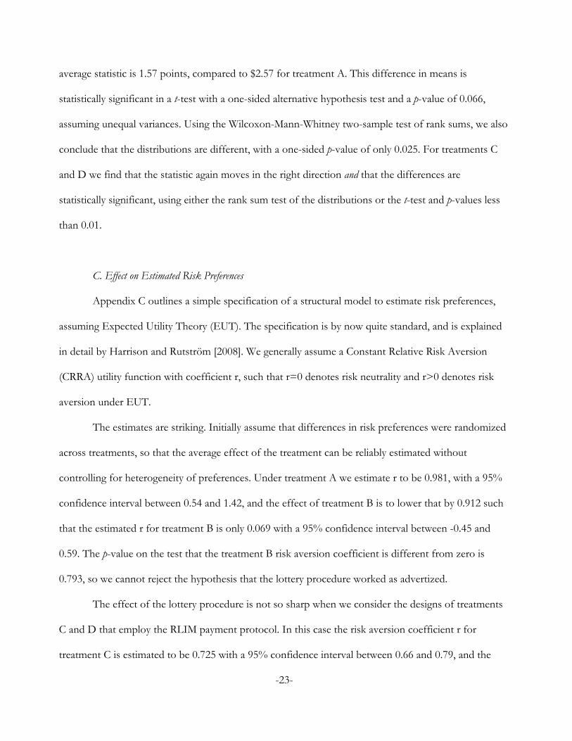
average statistic is 1.57 points, compared to $2.57 for treatment A. This difference in means is

statistically significant in a t-test with a one-sided alternative hypothesis test and a p-value of 0.066,

assuming unequal variances. Using the Wilcoxon-Mann-Whitney two-sample test of rank sums, we also

conclude that the distributions are different, with a one-sided p-value of only 0.025. For treatments C

and D we find that the statistic again moves in the right direction and that the differences are

statistically significant, using either the rank sum test of the distributions or the t-test and p-values less

than 0.01.

C. Effect on Estimated Risk Preferences

Appendix C outlines a simple specification of a structural model to estimate risk preferences,

assuming Expected Utility Theory (EUT). The specification is by now quite standard, and is explained

in detail by Harrison and Rutström [2008]. We generally assume a Constant Relative Risk Aversion

(CRRA) utility function with coefficient r, such that r=0 denotes risk neutrality and r>0 denotes risk

aversion under EUT.

The estimates are striking. Initially assume that differences in risk preferences were randomized

across treatments, so that the average effect of the treatment can be reliably estimated without

controlling for heterogeneity of preferences. Under treatment A we estimate r to be 0.981, with a 95%

confidence interval between 0.54 and 1.42, and the effect of treatment B is to lower that by 0.912 such

that the estimated r for treatment B is only 0.069 with a 95% confidence interval between -0.45 and

0.59. The p-value on the test that the treatment B risk aversion coefficient is different from zero is

0.793, so we cannot reject the hypothesis that the lottery procedure worked as advertized.

The effect of the lottery procedure is not so sharp when we consider the designs of treatments

C and D that employ the RLIM payment protocol. In this case the risk aversion coefficient r for

treatment C is estimated to be 0.725 with a 95% confidence interval between 0.66 and 0.79, and the

-23-

effect of the lottery procedure is to lower that by 0.45. Hence the estimated risk aversion coefficient

under treatment D is 0.161, with a 95% confidence interval between 0.15 and 0.17, and a p-value on the

one-sided hypothesis of risk neutrality of only 0.032. So we observe clear movement in the direction of

risk neutrality, but not the attainment of risk neutrality. The estimated effect of the lottery procedure, -

0.45, has a 95% confidence interval between -0.75 and -0.15.

We can extend these structural models to provide some allowance for subject heterogeneity.

Because the data for each subject in treatments A and B consist of just one observation, one loses

degrees of freedom rapidly with too many demographic characteristics. For example, in samples of 55,

how many Asian females are Seniors? Larger samples would obviously mitigate this issue, but for

present purposes a simpler solution is to merge in data from comparable tasks and samples drawn at

random from the same population. In this case we were able to use data for treatment A using lotteries

that use the same prizes and probabilities, but in different combinations than the 24 we focus on in the

comparisons of choice patterns.21 This increases the sample size for estimation from 55 to 149 under

treatment A.22 This is not appropriate when one is comparing choice patterns, since the stimuli are

different in nature, but is appropriate when one is estimating risk preferences.

Allowing for subject heterogeneity confirms our qualitative conclusions from assuming that

randomization to treatment led to the same distribution of preferences across treatments. Detailed

estimation results are provided in Appendix C, and control for a number of binary characteristics: blp

is 1 for choices in treatment B or treatment D; female is 1 for women, and 0 otherwise; sophomore

and senior are 1 for whether that was the current stage of undergraduate education at GSU, and 0

otherwise; and asian and white are 1 based on self-reported ethnic status, and 0 otherwise.

21 The additional lotteries are documented in Harrison and Swarthout [2012].22 The fraction of choices consistent with risk neutrality drops slightly, from 60.0% to 58.4%., with

the enhanced sample.

-24-

Controlling for observable characteristics in this manner, for treatments A and B we estimate

the coefficient on the lottery procedure dummy to be -0.70, with a p-value of 0.034, and the constant

term for treatment A to be 0.74 with a p-value of less than 0.001. The net effect, the estimated

coefficient for treatment B after controlling for the demographic covariates, is -0.042 with a p-value of

0.90, so we again cannot reject the null hypothesis that the lottery procedure induces risk neutral

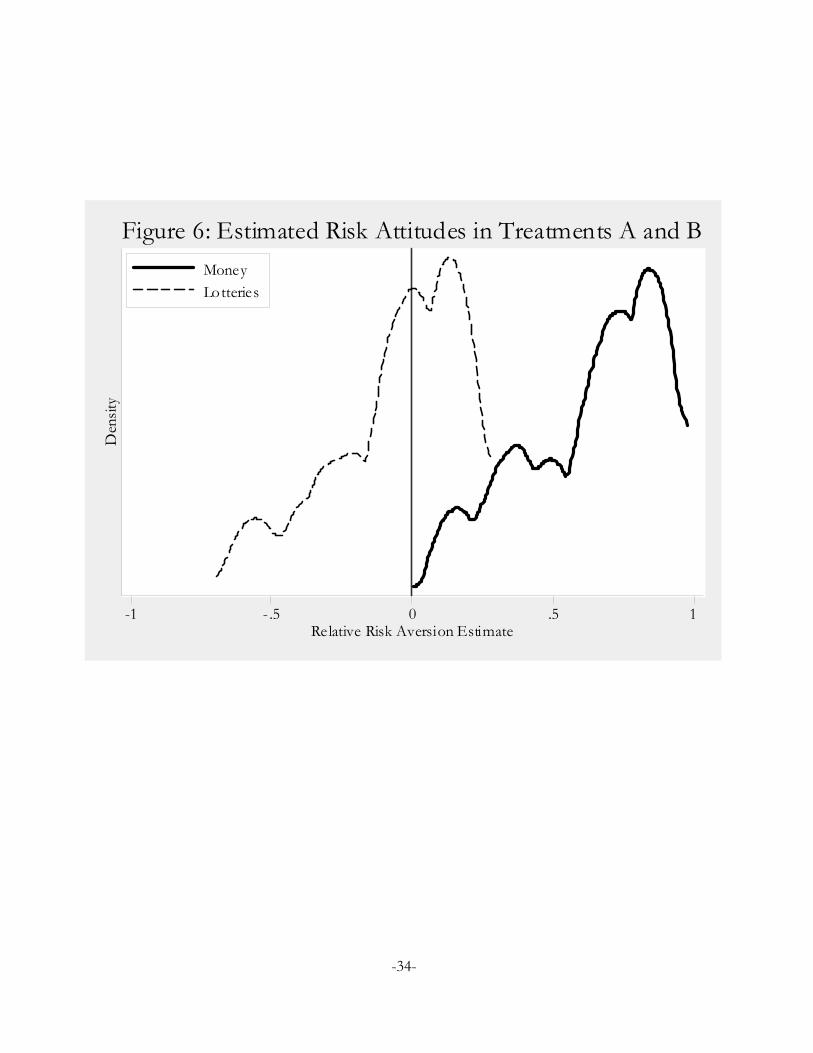
behavior. Predicting risk attitudes using these estimates, the average r for treatment A is 0.63, and for

treatment B is -0.077. Figure 6 displays kernel densities of the predicted risk attitudes over all subjects,

demonstrating the dramatic effect of the binary lottery procedure. These conclusions stay the same if

we pool in the choices from treatments E and F; again, the normative variants in the binary lottery

procedure displays and instructions do not, by themselves, make much of a difference.

For treatments C and D we estimate the effect of the lottery procedure on the risk aversion

coefficient to be -0.48 with a p-value of 0.003, compared to the constant term of 0.67 with a p-value

also less than 0.001. So the net effect, demographics aside, is for the lottery procedure to lower the

estimated risk aversion to 0.20 with a 95% confidence interval between -0.14 and 0.53 and a p-value of

0.25. Figure 7 shows the distribution of estimated risk attitudes from predicted values that account for

heterogeneity of preferences. The average predicted risk aversion in treatment C is 0.73 and in

treatment D is 0.26. The effect is not as complete as estimated for treatments A and B, but clearly in

the predicted direction.

5. Conclusions

Our results clearly show that the binary lottery procedure works for samples of university level

students in the simplest possible environment, where we can be certain that there are no contaminating

factors and the theory to be tested requires no auxiliary assumptions. This does not automatically make

the lottery procedure useful for samples from different populations. Nor does it automatically mean

-25-

that it applies in all settings, since it is often the “contaminating factor,” such as strategic behavior, that

is precisely the domain where we would like it to work. But there are many circumstances where one

can implement the environment considered here.

We find that the lottery procedure works robustly to induce risk neutrality when subjects are

given one task, and that it works well when subjects are given more than one task. The extent to which

the procedure works is certainly diminished as one moves from environments with one task to

environments with many tasks, but there is always a statistically significant reduction in risk aversion,

and in neither case can one reject the hypothesis that the procedure induced risk neutral behavior as

advertized.

Our results should encourage efforts to actively try to find procedures that can identify and

increase the sub-sample of subjects for whom the lottery procedure does induce linear utility, and the

populations for which it appears to work reliably.23 Even with a given population, it is logically possible

that the procedure “works as advertized” for some subjects, just not all, or even for a majority. There

can still be value in identifying those subjects. Moreover, if simple treatments can increase that fraction,

or just improve the statistical identification of that fraction, then we might discover a “best practice”

variant of the basic lottery procedure. Although the variants we considered in our design did not

increase the faction of risk neutral choices significantly, they could play a behavioral role in other

populations.

23 For example, Hossain and Okui [2011] evaluate the procedure in the context of eliciting theprobability of a binary event.

-26-

Table 1: Experimental Design

All choices drawn from the same battery of 24 lottery pairs at random.All subjects receive a $7.50 show-up fee.

Subjects were told that there would be no other salient task in the experiment.

TreatmentSubjects(Choices)

A. Monetary prizes with only one binary choice (Figure 3) 55(55)

B. Binary lottery points with only one binary choice (Figure 4) 69(69)

C. Monetary prizes with one binary choice out of Ko1 selected forpayment (Figure 3)

208(2104)

D. Binary lottery points with one binary choice out of Ko1 selected forpayment (Figure 4)

39(936)

E. Binary lottery points with only one binary choice and with EVinformation provided for each lottery (Figure 5)

34(34)

F. Binary lottery points with only one binary choice and with EVinformation provided for each lottery (Figure 5), as well as “cheaptalk” instructions

38(38)

-27-

Figure 1: Graphical Representation of Compound Lottery A and its Actuarially-Equivalent Lottery X

-28-

Figure 2: Graphical Representation of the Compound Version of a Binary Lotteryand its Actuarially-Equivalent Lottery

-29-

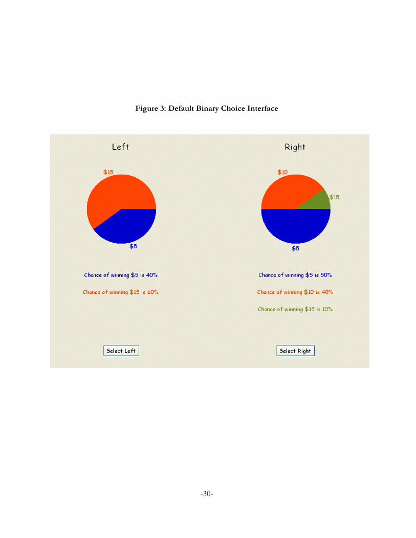
Figure 3: Default Binary Choice Interface

-30-

Figure 4: Choice Interface for Points

-31-

Figure 5: Choice Interface for Points with Expected Value Information

-32-

Table 2: Observed Choice Patterns

TreatmentRisk neutral

choices Other

choicesAll

choices

A. Monetary prizes with one choice (Figure 3) 33(60%)

22(40%)

55(100%)

B. Binary lottery points with one choice (Figure 4) 51(74%)

18(26%)

69(100%)

C. Monetary prizes with Ko1 choices (Figure 3) 1,336(63%)

768(37%)

2,104(100%)

D. Binary lottery points with Ko1 choices (Figure 4) 643(69%)

293(31%)

936(100%)

E. Binary lottery points with one choice and EVinformation (Figure 5)

24(71%)

10(29%)

34(100%)

F. Binary lottery points with one choice and EVinformation (Figure 5), plus “cheap talk”instructions

30(79%)

8(21%)

38(100%)

-33-

Den

sity

-1 - .5 0 .5 1Relative Risk Aversion Estimate

MoneyLotteries

Figure 6: Estimated Risk Attitudes in Treatments A and B

-34-

Den

sity

-.25 0 .25 .5 .75 1Relative Risk Aversion Estimate

MoneyLotteries

Figure 7: Estimated Risk Attitudes in Treatments C and D

-35-

References

Beattie, J., and Loomes, Graham, “The Impact of Incentives Upon Risky Choice Experiments,” Journalof Risk and Uncertainty, 14, 1997, 149-162.

Berg, Joyce E.; Daley, Lane A.; Dickhaut, John W.; and O’Brien, John R., “Controlling Preferences forLotteries on Units of Experimental Exchange,” Quarterly Journal of Economics, 101, May 1986,281-306.

Berg, Joyce E.; Rietz, Thomas A., and Dickhaut, John W., “On the Performance of the LotteryProcedure for Controlling Risk Preferences,” in C.R. Plott and V.L. Smith (eds.), Handbook ofExperimental Economics Results (New York: Elsevier Press, 2008).

Braunstein, Yale M., and Schotter, Andrew, “Labor Market Search: An Experimental Study,” EconomicInquiry, 20, January 1982, 133-144.

Cooper, Russell; DeJong, Douglas V.; Forsythe, Robert, and Ross, Thomas W., “Communication in theBattle of the Sexes Game: Some Experimental Results,” Rand Journal of Economics, 20, Winter1989, pp. 568-587.

Cooper, Russell; DeJong, Douglas V.; Forsythe, Robert, and Ross, Thomas W., “Selection Criteria inCoordination Games: Some Experimental Results,” American Economic Review, 80, March 1990,pp. 218-233.

Cooper, Russell; DeJong, Douglas V.; Forsythe, Robert, and Ross, Thomas W., “Communication inCoordination Games,” Quarterly Journal of Economics, 107, May 1992, 739-771.

Cooper, Russell; DeJong, Douglas V.; Forsythe, Robert, and Ross, Thomas W., “Forward Induction inthe Battle-of-Sexes Games,” American Economic Review, 83(5), December 1993, 1303-1316.

Cox, James C., and Oaxaca, Ronald L., “Inducing Risk-Neutral Preferences: Further Analysis of theData,” Journal of Risk and Uncertainty, 11, 1995, 65-79.

Cox, James C.; Sadiraj, Vjollca, and Schmidt, Ulrich, “Paradoxes and Mechanisms for Choice underRisk,” Working Paper 2011-12, Center for the Economic Analysis of Risk, Robinson College ofBusiness, Georgia State University, 2011.

Cox, James C.; Smith, Vernon L.; and Walker, James M., “Experimental Development of Sealed-BidAuction Theory: Calibrating Controls for Risk Aversion,” American Economic Review (Papers &Proceedings), 75, May 1985, 160-165.

Cubitt, Robin P.; Starmer, Chris, and Sugden, Robert, “On the Validity of the Random LotteryIncentive System,” Experimental Economics, 1(2), 1998, 115-131.

Harrison, Glenn W., “Theory and Misbehavior of First-Price Auctions,” American Economic Review, 79,September 1989, 749-762.

-36-

Harrison, Glenn W., “Theory and Misbehavior of First-Price Auctions: Reply,” American EconomicReview, 82, December 1992, 1426-1443.

Harrison, Glenn W., “Expected Utility Theory and the Experimentalists,” Empirical Economics, 19(2),1994, 223-253; reprinted in J.D. Hey (ed.), Experimental Economics (Heidelberg: Physica-Verlag,1994).

Harrison, Glenn W., and McCabe, Kevin, “Testing Noncooperative Bargaining Theory inExperiments,” in R.M. Isaac (ed.), Research in Experimental Economics (Greenwich: JAI Press,Volume 5, 1992).

Harrison, Glenn W., and McCabe, Kevin A., “Expectations and Fairness in a Simple BargainingExperiment,” International Journal of Game Theory, 25(3), 1996, 303-327.

Harrison, Glenn W., and Rutström, E. Elisabet, “Trade Wars, Trade Negotiations, and Applied GameTheory,” Economic Journal, 101, May 1991, 420-435.

Harrison, Glenn W., and Rutström, E. Elisabet, “Risk Aversion in the Laboratory,” in J.C. Cox andG.W. Harrison (eds.), Risk Aversion in Experiments (Bingley, UK: Emerald, Research inExperimental Economics, Volume 12, 2008).

Harrison, Glenn W., and Swarthout, J. Todd, “Independence and the Bipolar Behaviorist,” WorkingPaper 2012-01, Center for the Economic Analysis of Risk, Robinson College of Business,Georgia State University, 2012.

Holt, Charles A., and Laury, Susan K., “Risk Aversion and Incentive Effects,” American Economic Review,92(5), December 2002, 1644-1655.

Hossain, Tanjim, and Okui, Ryo, “The Binarized Scoring Rule,” Working Paper, University of Toronto,August 2011.

Machina, Mark J., and Schmeidler, David, “A More Robust Definition of Subjective Probability,”Econometrica, 60(4), July 1992, 745-780.

Machina, Mark J., and Schmeidler, David, “Bayes without Bernoulli: Simple Conditions forProbabilistically Sophisticated Choice,” Journal of Economic Theory, 67, 1995, 106-128.

Ochs, Jack, and Roth, Alvin E., “An Experimental Study of Sequential Bargaining,” American EconomicReview, 79(3), June 1989, 355-384.

Rao, J. N. K., and Scott, A. J., “On Chi-squared Tests for Multiway Contingency Tables with CellProportions Estimated from Survey Data,” Annals of Statistics, 12, 1984, 46-60.

Rietz, Thomas A., “Implementing and Testing Risk Preference Induction Mechanisms in ExperimentalSealed Bid Auctions,” Journal of Risk and Uncertainty, 7, 1993, 199-213.

-37-

Roth, Alvin E., and Malouf, Michael W. K., “Game-Theoretic Models and the Role of Information inBargaining,” Psychological Review, 86, 1979, 574-594.

Samuelson, Paul A., “Probability, Utility, and the Independence Axiom,” Econometrica, 20, 1952, 670-678.

Savage, Leonard J., The Foundations of Statistics (New York: John Wiley, 1954).

Savage, Leonard J., The Foundations of Statistics (New York: Dover Publications, 1972; Second Edition).

Segal, Uzi, “Does the Preference Reversal Phenomenon Necessarily Contradict the IndependenceAxiom?” American Economic Review, 78(1), March 1988, 233-236.

Segal, Uzi, “Two-Stage Lotteries Without the Reduction Axiom,” Econometrica, 58(2), March 1990, 349-377.

Segal, Uzi, “The Independence Axiom Versus the Reduction Axiom: Must We Have Both?” in W.Edwards (ed.), Utility Theories: Measurements and Applications (Boston: Kluwer AcademicPublishers, 1992).

Selten, Reinhard; Sadrieh, Abdolkarim, and Abbink, Klaus, “Money Does Not Induce Risk NeutralBehavior, but Binary Lotteries Do even Worse,” Theory and Decision, 46(3), June 1999, 211-249.

Smith, Cedric A.B., “Consistency in Statistical Inference and Decision,” Journal of the Royal StatisticalSociety, 23, 1961, 1-25.

Starmer, Chris, and Sugden, Robert, “Does the Random-Lottery Incentive System Elicit TruePreferences? An Experimental Investigation,” American Economic Review, 81, 1991, 971-978.

Walker, James M.; Smith, Vernon L., and Cox, James C., “Inducing Risk Neutral Preferences: AnExamination in a Controlled Market Environment,” Journal of Risk and Uncertainty, 3, 1990, 5-24.

Wilcox, Nathaniel T., “A Comparison of Three Probabilistic Models of Binary Discrete Choice UnderRisk,” Working Paper, Economic Science Institute, Chapman University, March 2010.

-38-

Appendix A: Instructions (NOT FOR PUBLICATION)

Treatment AChoices Over Risky Prospects

This is a task where you will choose between prospects with varying prizes and chances ofwinning. You will be presented with one pair of prospects where you will choose one of them. Youshould choose the prospect you prefer to play. You will actually get the chance to play the prospect youchoose, and you will be paid according to the outcome of that prospect, so you should think carefullyabout which prospect you prefer.

Here is an example of what the computer display of a pair of prospects will look like.

The outcome of the prospects will be determined by the draw of a random number between 1and 100. Each number between, and including, 1 and 100 is equally likely to occur. In fact, you will beable to draw the number yourself using two 10-sided dice.

In the above example the left prospect pays five dollars ($5) if the number drawn is between 1and 40, and pays fifteen dollars ($15) if the number is between 41 and 100. The blue color in the pie

-39-

chart corresponds to 40% of the area and illustrates the chances that the number drawn will be between1 and 40 and your prize will be $5. The orange area in the pie chart corresponds to 60% of the area andillustrates the chances that the number drawn will be between 41 and 100 and your prize will be $15.

Now look at the pie in the chart on the right. It pays five dollars ($5) if the number drawn isbetween 1 and 50, ten dollars ($10) if the number is between 51 and 90, and fifteen dollars ($15) if thenumber is between 91 and 100. As with the prospect on the left, the pie slices represent the fraction ofthe possible numbers which yield each payoff. For example, the size of the $15 pie slice is 10% of thetotal pie.

The pair of prospects you choose from is shown on a screen on the computer. On that screen,you should indicate which prospect you prefer to play by clicking on one of the buttons beneath theprospects.

After you have made your choice, raise your hand and an experimenter will come over. It iscertain that your one choice will be played out for real. You will roll the two ten-sided dice to determinethe outcome of the prospect you chose.

For instance, suppose you picked the prospect on the left in the above example. If the randomnumber was 37, you would win $5; if it was 93, you would get $15. If you picked the prospect on theright and drew the number 37, you would get $5; if it was 93, you would get $15.

Therefore, your payoff is determined by two things:

• by which prospect you selected, the left or the right; and • by the outcome of that prospect when you roll the two 10-sided dice.

Which prospects you prefer is a matter of personal taste. The people next to you may be presented witha different prospect, and may have different preferences, so their responses should not matter to you.Please work silently, and make your choices by thinking carefully about the prospect you are presentedwith.

All payoffs are in cash, and are in addition to the $7.50 show-up fee that you receive just forbeing here. The only other task today is for you to answer some demographic questions. Your answersto those questions will not affect your payoffs.

Treatment B

Choices Over Risky Prospects

This is a task where you will choose between prospects with varying chances of winning either ahigh amount or a low amount. You will be presented with one pair of prospects where you will chooseone of them. You should choose the prospect you prefer to play. You will actually get the chance toplay the prospect you choose, and you will be paid according to the final outcome of that prospect, soyou should think carefully about which prospect you prefer.

Here is an example of what the computer display of a pair of prospects will look like.

-40-

You earn points in this task. We explain below how points are converted to cash payoffs.

The outcome of the prospects will be determined by the draw of two random numbers between1 and 100. The first random number drawn determines the number of points you earn in the chosenprospect, and the second random number determines whether you win the high or the low amountaccording to the points earned. The high amount is $100 and the low amount is $0. Each randomnumber between, and including, 1 and 100 is equally likely to occur. In fact, you will be able to draw thetwo random numbers yourself by rolling two 10-sided dice twice.

The payoffs in each prospect are points that give you the chance of winning the $100 highamount. The more points you earn, the greater your chance of winning $100. In the left prospect of theabove example you earn five points (5) if the outcome of the first dice roll is between 1 and 25, twentypoints (20) if the outcome of the dice roll is between 26 and 75, and seventy points (70) if the outcomeof the roll is between 76 and 100. The blue color in the pie chart corresponds to 25% of the area andillustrates the chances that the number drawn will be between 1 and 25 and your prize will be 5 points.The orange area in the pie chart corresponds to 50% of the area and illustrates the chances that thenumber drawn will be between 26 and 75 and your prize will be 20 points. Finally, the green area in thepie chart corresponds to the remaining 25% of the area and illustrates that the number drawn will be

-41-

between 76 and 100 and your prize is 70 points.

Now look at the pie in the chart on the right. You earn five points (5) if the first number drawnis between 1 and 50 and seventy points (70) if the number is between 51 and 100. As with the prospecton the left, the pie slices represent the fraction of the possible numbers which yield each payoff. Forexample, the size of the 5 points pie slice is 50% of the total pie.

Every point that you earn gives you greater chance of being paid for this task. If you earn 70points then you have a 70% chance of being paid $100. If you earn 20 points then you have a 20%chance of being paid $100. After you determine the number of points that you earn by rolling the two10-sided dice once, you will then roll the same dice for a second time to determine if you get $100 or$0. If your second roll is a number that is less than or equal to the number of points that you earned,you win $100. If the second roll is a number that is greater than the number of points that you earned,you get $0. If you do not win $100 you receive nothing from this task, but of course you get to keepyour show-up fee. Again, the more points you earn the greater your chance of winning $100 in thistask.

The pair of prospects you choose from is shown on a screen on the computer. On that screen,you should indicate which prospect you prefer to play by clicking on one of the buttons beneath theprospects.

After you have made your choice, raise your hand and an experimenter will come over. It iscertain that your one choice will be played out for real. You will then roll the two ten-sided dice twice:first to determine the number of points you win, and then to determine whether you win $100 or $0according to the points earned.

For instance, suppose you picked the prospect on the left in the above example. If the outcomeof the first dice roll was 17, you would win 5 points. This means that your chance of winning $100 is5%. Now, if the outcome of the second dice roll was 1, which is less than the number of points youearned, you would win $100. If the second roll was 75 instead, you would earn nothing because theoutcome of this roll is greater than the number of points you earned.

Here is another example. If you picked the prospect on the right and the outcome of the firstdice roll was 60, then you would earn 70 points. This means that your probability of winning $100would be 70%. If the outcome of the second dice roll was 1, then you would earn $100; but if thesecond roll was 75 instead you would earn $0 in this task.

Therefore, your payoff is determined by three things:

• the prospect you selected, the left or the right;• the outcome of the first roll of the two 10-sided dice which determines the number of points

your earn in your chosen prospect; and• the outcome of the second roll of the two 10-sided dice which will be compared with your

earned points to determine whether you earn $0 or $100.

Which prospect you prefer is a matter of personal taste. The people next to you may be presented witha different pair of prospects, so their responses should not matter to you. Please work silently, and

-42-

make your choices by thinking carefully about the pair of prospects you are presented with.

All payoffs are in cash, and are in addition to the $7.50 show-up fee that you receive just forbeing here. The only other task today is for you to answer some demographic questions. Your answersto those questions will not affect your payoffs.

Treatment C

Choices Over Risky Prospects

This is a task where you will choose between prospects with varying prizes and chances ofwinning. You will be presented with a series of pairs of prospects where you will choose one of them.There are 30 pairs in the series. For each pair of prospects, you should choose the prospect you preferto play. You will actually get the chance to play one of the prospects you choose, and you will be paidaccording to the outcome of that prospect, so you should think carefully about which prospect youprefer.

Here is an example of what the computer display of such a pair of prospects will look like.

SAME DISPLAY AS FOR TREATMENT A

The outcome of the prospects will be determined by the draw of a random number between 1and 100. Each number between, and including, 1 and 100 is equally likely to occur. In fact, you will beable to draw the number yourself using two 10-sided dice.

In the above example the left prospect pays five dollars ($5) if the number drawn is between 1and 40, and pays fifteen dollars ($15) if the number is between 41 and 100. The blue color in the piechart corresponds to 40% of the area and illustrates the chances that the number drawn will be between1 and 40 and your prize will be $5. The orange area in the pie chart corresponds to 60% of the area andillustrates the chances that the number drawn will be between 41 and 100 and your prize will be $15.

Now look at the pie in the chart on the right. It pays five dollars ($5) if the number drawn isbetween 1 and 50, ten dollars ($10) if the number is between 51 and 90, and fifteen dollars ($15) if thenumber is between 91 and 100. As with the prospect on the left, the pie slices represent the fraction ofthe possible numbers which yield each payoff. For example, the size of the $15 pie slice is 10% of thetotal pie.

Each pair of prospects is shown on a separate screen on the computer. On each screen, youshould indicate which prospect you prefer to play by clicking on one of the buttons beneath theprospects.

After you have worked through all of the pairs of prospects, raise your hand and anexperimenter will come over. You will then roll a 30-sided die to determine which pair of prospects will be played out. Since there is a chance that any of your 30 choices could be played out for real, youshould approach each pair of prospects as if it is the one that you will play out. Finally, you will roll thetwo ten-sided dice to determine the outcome of the prospect you chose.

-43-

For instance, suppose you picked the prospect on the left in the above example. If the randomnumber was 37, you would win $5; if it was 93, you would get $15. If you picked the prospect on theright and drew the number 37, you would get $5; if it was 93, you would get $15.

Therefore, your payoff is determined by three things:

• by which prospect you selected, the left or the right, for each of these 30 pairs; • by which prospect pair is chosen to be played out in the series of 30 such pairs using the

30-sided die; and • by the outcome of that prospect when you roll the two 10-sided dice.

Which prospects you prefer is a matter of personal taste. The people next to you may be presented withdifferent prospects, and may have different preferences, so their responses should not matter to you.Please work silently, and make your choices by thinking carefully about each prospect.

All payoffs are in cash, and are in addition to the $7.50 show-up fee that you receive just forbeing here. The only other task today is for you to answer some demographic questions. Your answersto those questions will not affect your payoffs.

Treatment D

Choices Over Risky Prospects

This is a task where you will choose between prospects with varying chances of winning either ahigh amount or a low amount. You will be presented with a series of pairs of prospects where you willchoose one of them. There are 24 pairs in the series. For each pair of prospects, you should choose theprospect you prefer to play. You will actually get the chance to play one of the prospects you choose,and you will be paid according to the final outcome of that prospect, so you should think carefullyabout which prospect you prefer.

Here is an example of what the computer display of a pair of prospects will look like.

SAME DISPLAY AS FOR TREATMENT B

You earn points in this task. We explain below how points are converted to cash payoffs.

The outcome of the prospects will be determined by the draw of two random numbers between1 and 100. The first random number drawn determines the number of points you earn in the chosenprospect, and the second random number determines whether you win the high or the low amountaccording to the points earned. The high amount is $100 and the low amount is $0. Each randomnumber between, and including, 1 and 100 is equally likely to occur. In fact, you will be able to draw thetwo random numbers yourself by rolling two 10-sided dice twice.

The payoffs in each prospect are points that give you the chance of winning the $100 highamount. The more points you earn, the greater your chance of winning $100. In the left prospect of theabove example you earn five points (5) if the outcome of the first dice roll is between 1 and 25, twentypoints (20) if the outcome of the dice roll is between 26 and 75, and seventy points (70) if the outcome

-44-

of the roll is between 76 and 100. The blue color in the pie chart corresponds to 25% of the area andillustrates the chances that the number drawn will be between 1 and 25 and your prize will be 5 points.The orange area in the pie chart corresponds to 50% of the area and illustrates the chances that thenumber drawn will be between 26 and 75 and your prize will be 20 points. Finally, the green area in thepie chart corresponds to the remaining 25% of the area and illustrates that the number drawn will bebetween 76 and 100 and your prize is 70 points.

Now look at the pie in the chart on the right. You earn five points (5) if the first number drawnis between 1 and 50 and seventy points (70) if the number is between 51 and 100. As with the prospecton the left, the pie slices represent the fraction of the possible numbers which yield each payoff. Forexample, the size of the 5 points pie slice is 50% of the total pie.

Every point that you earn gives you greater chance of being paid for this task. If you earn 70points then you have a 70% chance of being paid $100. If you earn 20 points then you have a 20%chance of being paid $100. After you determine the number of points that you earn by rolling the two10-sided dice once, you will then roll the same dice for a second time to determine if you get $100 or$0. If your second roll is a number that is less or equal to the number of points that you earned, youwin $100. If the second roll is a number that is greater than the number of points that you earned, youget $0. If you do not win $100 you receive nothing from this task, but of course you get to keep yourshow-up fee. Again, the more points you earn the greater your chance of winning $100 in this task.

Each pair of prospects is shown on a separate screen on the computer. On each screen, youshould indicate which prospect you prefer to play by clicking on one of the buttons beneath theprospects.

After you have worked through all of the pairs of prospects, raise your hand and anexperimenter will come over. You will then roll a 30-sided die until a number between 1 and 24 comesup to determine which pair of prospects will be played out for real. Since there is a chance that any ofyour 24 choices could be played out for real, you should approach each pair of prospects as if it is theone that you will play out. Finally, you will then roll the two ten-sided dice twice: first to determine thenumber of points you win, and then to determine whether you win $100 or $0 according to the pointsearned.

For instance, suppose you picked the prospect on the left in the above example. If the outcomeof the first dice roll was 17, you would win 5 points. This means that your chance of winning $100 is5%. Now, if the outcome of the second dice roll was 1, which is less than the number of points youearned, you would win $100. If the second roll was 75 instead, you would earn nothing because theoutcome of this roll is greater than the number of points you earned.

Here is another example. If you picked the prospect on the right and the outcome of the firstdice roll was 60, then you would earn 70 points. This means that your probability of winning $100would be 70%. If the outcome of the second dice roll was 1, then you would earn $100; but if thesecond roll was 75 instead you would earn $0 in this task.

Therefore, your payoff is determined by four things:

• the prospect you selected, the left or the right, for each of these 24 pairs;

-45-

• the prospect pair that is chosen to be played out in the series of 24 such pairs using the 30-sideddie;

• the outcome of the first roll of the two 10-sided dice which determines the number of pointsyour earn in your chosen prospect; and

• the outcome of the second roll of the two 10-sided dice which will be compared with yourearned points to determine whether you earn $0 or $100.

Which prospect you prefer is a matter of personal taste. The people next to you may be presented withdifferent prospects, so their responses should not matter to you. Please work silently, and make yourchoices by thinking carefully about the pair of prospects you are presented with.

All payoffs are in cash, and are in addition to the $7.50 show-up fee that you receive just forbeing here. The only other task today is for you to answer some demographic questions. Your answersto those questions will not affect your payoffs.

Treatment E

SAME INSTRUCTIONS AS FOR TREATMENT B, WITH ADDITIONS PRESENTEDIN THE TEXT AND USING DISPLAY IN FIGURE 5.

Treatment F

SAME INSTRUCTIONS AS FOR TREATMENT E, WITH ADDITIONS PRESENTEDIN THE TEXT AND USING DISPLAY IN FIGURE 5.

-46-

Appendix B: Parameters of Experiment

Table B1: Battery of Monetary Lotteries

Prizes “Safe” Lottery Probabilities “Risky” Lottery ProbabilitiesPair Context Low Middle High Low Middle High Low Middle High EV Safe EV Risky

1 5 $5 $20 $70 0 0.75 0.25 0.25 0 0.75 $32.50 $53.752 5 $5 $20 $70 0.25 0.5 0.25 0.5 0 0.5 $28.75 $37.503 5 $5 $20 $70 0 0.5 0.5 0.25 0 0.75 $45.00 $53.754 6 $5 $35 $70 0 1 0 0.25 0 0.75 $35.00 $53.755 6 $5 $35 $70 0.25 0.75 0 0.5 0 0.5 $27.50 $37.506 6 $5 $35 $70 0 0.75 0.25 0.25 0 0.75 $43.75 $53.757 6 $5 $35 $70 0 0.5 0.5 0.25 0 0.75 $52.50 $53.758 6 $5 $35 $70 0 0.75 0.25 0.5 0 0.5 $43.75 $37.509 9 $10 $35 $70 0 1 0 0.25 0 0.75 $35.00 $55.0010 9 $10 $35 $70 0.25 0.75 0 0.5 0 0.5 $28.75 $40.0011 9 $10 $35 $70 0 0.5 0.5 0.25 0 0.75 $52.50 $55.0012 9 $10 $35 $70 0 0.75 0.25 0.5 0 0.5 $43.75 $40.0013 10 $20 $35 $70 0 1 0 0.25 0 0.75 $35.00 $57.5014 10 $20 $35 $70 0.25 0.75 0 0.5 0 0.5 $31.25 $45.0015 10 $20 $35 $70 0 0.75 0.25 0.25 0 0.75 $43.75 $57.5016 10 $20 $35 $70 0 1 0 0.5 0 0.5 $35.00 $45.0017 10 $20 $35 $70 0.5 0.5 0 0.75 0 0.25 $27.50 $32.5018 10 $20 $35 $70 0 1 0 0.25 0.5 0.25 $35.00 $40.0019 10 $20 $35 $70 0.25 0.5 0.25 0.5 0 0.5 $40.00 $45.0020 10 $20 $35 $70 0 0.5 0.5 0.25 0 0.75 $52.50 $57.5021 10 $20 $35 $70 0 1 0 0.5 0.25 0.25 $35.00 $36.2522 10 $20 $35 $70 0.25 0.75 0 0.75 0 0.25 $31.25 $32.5023 10 $20 $35 $70 0 0.75 0.25 0.5 0 0.5 $43.75 $45.0024 10 $20 $35 $70 0 1 0 0.75 0 0.25 $35.00 $32.50

-47-

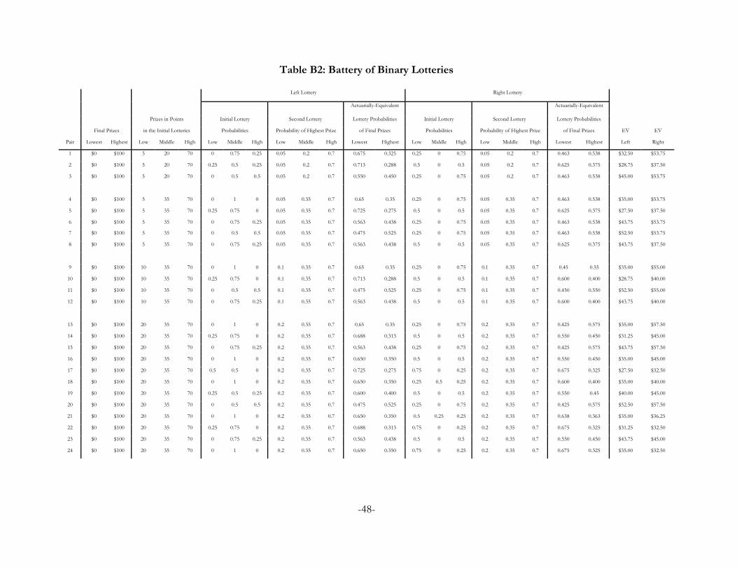
Table B2: Battery of Binary Lotteries

Left Lottery Right Lottery

Actuarially-Equivalent Actuarially-Equivalent

Prizes in Points Initial Lottery Second Lottery Lottery Probabilities Initial Lottery Second Lottery Lottery Probabilities

Final Prizes in the Initial Lotteries Probabilities Probability of Highest Prize of Final Prizes Probabilities Probability of Highest Prize of Final Prizes EV EV

Pair Lowest Highest Low Middle High Low Middle High Low Middle High Lowest Highest Low Middle High Low Middle High Lowest Highest Left Right

1 $0 $100 5 20 70 0 0.75 0.25 0.05 0.2 0.7 0.675 0.325 0.25 0 0.75 0.05 0.2 0.7 0.463 0.538 $32.50 $53.75

2 $0 $100 5 20 70 0.25 0.5 0.25 0.05 0.2 0.7 0.713 0.288 0.5 0 0.5 0.05 0.2 0.7 0.625 0.375 $28.75 $37.50

3 $0 $100 5 20 70 0 0.5 0.5 0.05 0.2 0.7 0.550 0.450 0.25 0 0.75 0.05 0.2 0.7 0.463 0.538 $45.00 $53.75

4 $0 $100 5 35 70 0 1 0 0.05 0.35 0.7 0.65 0.35 0.25 0 0.75 0.05 0.35 0.7 0.463 0.538 $35.00 $53.75

5 $0 $100 5 35 70 0.25 0.75 0 0.05 0.35 0.7 0.725 0.275 0.5 0 0.5 0.05 0.35 0.7 0.625 0.375 $27.50 $37.50

6 $0 $100 5 35 70 0 0.75 0.25 0.05 0.35 0.7 0.563 0.438 0.25 0 0.75 0.05 0.35 0.7 0.463 0.538 $43.75 $53.75

7 $0 $100 5 35 70 0 0.5 0.5 0.05 0.35 0.7 0.475 0.525 0.25 0 0.75 0.05 0.35 0.7 0.463 0.538 $52.50 $53.75

8 $0 $100 5 35 70 0 0.75 0.25 0.05 0.35 0.7 0.563 0.438 0.5 0 0.5 0.05 0.35 0.7 0.625 0.375 $43.75 $37.50

9 $0 $100 10 35 70 0 1 0 0.1 0.35 0.7 0.65 0.35 0.25 0 0.75 0.1 0.35 0.7 0.45 0.55 $35.00 $55.00

10 $0 $100 10 35 70 0.25 0.75 0 0.1 0.35 0.7 0.713 0.288 0.5 0 0.5 0.1 0.35 0.7 0.600 0.400 $28.75 $40.00

11 $0 $100 10 35 70 0 0.5 0.5 0.1 0.35 0.7 0.475 0.525 0.25 0 0.75 0.1 0.35 0.7 0.450 0.550 $52.50 $55.00

12 $0 $100 10 35 70 0 0.75 0.25 0.1 0.35 0.7 0.563 0.438 0.5 0 0.5 0.1 0.35 0.7 0.600 0.400 $43.75 $40.00

13 $0 $100 20 35 70 0 1 0 0.2 0.35 0.7 0.65 0.35 0.25 0 0.75 0.2 0.35 0.7 0.425 0.575 $35.00 $57.50

14 $0 $100 20 35 70 0.25 0.75 0 0.2 0.35 0.7 0.688 0.313 0.5 0 0.5 0.2 0.35 0.7 0.550 0.450 $31.25 $45.00

15 $0 $100 20 35 70 0 0.75 0.25 0.2 0.35 0.7 0.563 0.438 0.25 0 0.75 0.2 0.35 0.7 0.425 0.575 $43.75 $57.50

16 $0 $100 20 35 70 0 1 0 0.2 0.35 0.7 0.650 0.350 0.5 0 0.5 0.2 0.35 0.7 0.550 0.450 $35.00 $45.00

17 $0 $100 20 35 70 0.5 0.5 0 0.2 0.35 0.7 0.725 0.275 0.75 0 0.25 0.2 0.35 0.7 0.675 0.325 $27.50 $32.50

18 $0 $100 20 35 70 0 1 0 0.2 0.35 0.7 0.650 0.350 0.25 0.5 0.25 0.2 0.35 0.7 0.600 0.400 $35.00 $40.00

19 $0 $100 20 35 70 0.25 0.5 0.25 0.2 0.35 0.7 0.600 0.400 0.5 0 0.5 0.2 0.35 0.7 0.550 0.45 $40.00 $45.00

20 $0 $100 20 35 70 0 0.5 0.5 0.2 0.35 0.7 0.475 0.525 0.25 0 0.75 0.2 0.35 0.7 0.425 0.575 $52.50 $57.50

21 $0 $100 20 35 70 0 1 0 0.2 0.35 0.7 0.650 0.350 0.5 0.25 0.25 0.2 0.35 0.7 0.638 0.363 $35.00 $36.25

22 $0 $100 20 35 70 0.25 0.75 0 0.2 0.35 0.7 0.688 0.313 0.75 0 0.25 0.2 0.35 0.7 0.675 0.325 $31.25 $32.50

23 $0 $100 20 35 70 0 0.75 0.25 0.2 0.35 0.7 0.563 0.438 0.5 0 0.5 0.2 0.35 0.7 0.550 0.450 $43.75 $45.00

24 $0 $100 20 35 70 0 1 0 0.2 0.35 0.7 0.650 0.350 0.75 0 0.25 0.2 0.35 0.7 0.675 0.325 $35.00 $32.50

-48-

Appendix C: Structural Estimation of Risk Preferences (NOT FOR PUBLICATION)

Assume that utility of income is defined by

U(x) = x(1!r)/(1!r) (C1)

where x is the lottery prize and r…1 is a parameter to be estimated. For r=1 assume U(x)=ln(x) if

needed. Thus r is the coefficient of CRRA: r=0 corresponds to risk neutrality, r<0 to risk loving, and

r>0 to risk aversion. Let there be J possible outcomes in a lottery. Under EUT the probabilities for

each outcome xj, p(xj), are those that are induced by the experimenter, so expected utility is simply the

probability weighted utility of each outcome in each lottery i:

EUi = 3j=1,J [ p(xj) × U(xj) ]. (C2)

The EU for each lottery pair is calculated for a candidate estimate of r, and the index

LEU = EUR ! EUL (C3)

calculated, where EUL is the “left” lottery and EUR is the “right” lottery as presented to subjects. This

latent index, based on latent preferences, is then linked to observed choices using a standard cumulative

normal distribution function Φ(LEU). This “probit” function takes any argument between ±4 and

transforms it into a number between 0 and 1. Thus we have the probit link function,

prob(choose lottery R) = Φ(LEU) (C4)

Even though this “link function” is common in econometrics texts, it is worth noting explicitly and

understanding. It forms the critical statistical link between observed binary choices, the latent structure

generating the index LEU, and the probability of that index being observed. The index defined by (C3)

is linked to the observed choices by specifying that the R lottery is chosen when Φ(LEU)>½, which is

implied by (C4).

Thus the likelihood of the observed responses, conditional on the EUT and CRRA

specifications being true, depends on the estimates of r given the above statistical specification and the

observed choices. The “statistical specification” here includes assuming some functional form for the

-49-

cumulative density function (CDF). The conditional log-likelihood is then

ln L(r; y, X) = 3i [ (ln Φ(LEU)×I(yi = 1)) + (ln (1-Φ(LEU))×I(yi = !1)) ] (C5)

where I(@) is the indicator function, yi =1(!1) denotes the choice of the right (left) lottery in risk

aversion task i, and X is a vector of individual characteristics reflecting age, sex, race, and so on.

Harrison and Rutström [2008; Appendix F] review procedures that can be used to estimate

structural models of this kind, as well as more complex non-EUT models. The goal is to illustrate how

researches can write explicit maximum likelihood (ML) routines that are specific to different structural

choice models. It is a simple matter to correct for multiple responses from the same subject

(“clustering”), as needed.

It is also simple matter to generalize the ML analysis to allow the core parameter r to be a linear

function of observable characteristics of the individual or task. We extend the model to be r = r0 +

R×X, where r0 is a fixed parameter and R is a vector of effects associated with each characteristic in the

variable vector X. In effect the unconditional model assumes r = r0 and just estimates r0. This extension

significantly enhances the attraction of structural ML estimation, particularly for responses pooled over

different subjects and treatments, since one can condition estimates on observable characteristics of the

task or subject.

An important extension of the core model is to allow for subjects to make some behavioral

errors. The notion of error is one that has already been encountered in the form of the statistical

assumption that the probability of choosing a lottery is not 1 when the EU of that lottery exceeds the

EU of the other lottery. This assumption is clear in the use of a non-degenerate link function between

the latent index LEU and the probability of picking one or other lottery; in the case of the normal

CDF, this link function is Φ(LEU). If there were no errors from the perspective of EUT, this function

would be a step function: zero for all values of LEU<0, anywhere between 0 and 1 for LEU=0, and 1

for all values of LEU>0.

-50-

We employ the error specification originally due to Fechner and popularized by Hey and Orme

[1994]. This error specification posits the latent index

LEU = (EUR ! EUL)/μ (C3N)

instead of (C3), where μ is a structural “noise parameter” used to allow some errors from the

perspective of the deterministic EUT model. This is just one of several different types of error story

that could be used, and Wilcox [2008] provides a masterful review of the implications of the

alternatives.24 As μ60 this specification collapses to the deterministic choice EUT model, where the

choice is strictly determined by the EU of the two lotteries; but as μ gets larger and larger the choice

essentially becomes random. When μ=1 this specification collapses to (C3), where the probability of

picking one lottery is given by the ratio of the EU of one lottery to the sum of the EU of both lotteries.

Thus μ can be viewed as a parameter that flattens out the link functions as it gets larger.

An important contribution to the characterization of behavioral errors is the “contextual error”

specification proposed by Wilcox [2011]. It is designed to allow robust inferences about the primitive

“more stochastically risk averse than,” and posits the latent index

LEU = ((EUR ! EUL)/ν)/μ (C3O)

instead of (C3N), where ν is a new, normalizing term for each lottery pair L and R. The normalizing

term ν is defined as the maximum utility over all prizes in this lottery pair minus the minimum utility

over all prizes in this lottery pair. The value of ν varies, in principle, from lottery choice pair to lottery

choice pair: hence it is said to be “contextual.” For the Fechner specification, dividing by ν ensures that

the normalized EU difference [(EUR ! EUL)/ν] remains in the unit interval. The term ν does not need to

be estimated in addition to the utility function parameters and the parameter for the behavioral error

24 Some specifications place the error at the final choice between one lottery or after the subject hasdecided which one has the higher expected utility; some place the error earlier, on the comparison ofpreferences leading to the choice; and some place the error even earlier, on the determination of the expectedutility of each lottery.

-51-

tern, since it is given by the data and the assumed values of those estimated parameters.

The specification employed here is the CRRA utility function from (C1), the Fechner error

specification using contextual utility from (C3O), and the link function using the normal CDF from

(C4). The log-likelihood is then

ln L(r, μ; y, X) = 3i [ (ln Φ(LEU)×I(yi = 1)) + (ln (1-Φ(LEU))×I(yi = !1)) ] (C5N)

and the parameters to be estimated are r and μ given observed data on the binary choices y and the

lottery parameters in X.

Additional References

Hey, John D., and Orme, Chris, “Investigating Generalizations of Expected Utility Theory UsingExperimental Data,” Econometrica, 62(6), November 1994, 1291-1326.

Wilcox, Nathaniel T., “Stochastic Models for Binary Discrete Choice Under Risk: A Critical Primer andEconometric Comparison,” in J. Cox and G.W. Harrison (eds.), Risk Aversion in Experiments(Bingley, UK: Emerald, Research in Experimental Economics, Volume 12, 2008).

Wilcox, Nathaniel T., “‘Stochastically More Risk Averse:’ A Contextual Theory of Stochastic DiscreteChoice Under Risk,” Journal of Econometrics, 162(1), May 2011, 89-104.

-52-

Table C1: Estimation Results for Treatments A and B

Number of obs = 218 LR chi2(2) = 4.06Log likelihood = -117.39741 Prob > chi2 = 0.1316

------------------------------------------------------------------------------ | Coef. Std. Err. z P>|z| [95% Conf. Interval]-------------+----------------------------------------------------------------r | blp | -.7015267 .3317442 -2.11 0.034 -1.351733 -.0513201 female | .2341047 .2037852 1.15 0.251 -.165307 .6335164 sophomore | -.1999455 .2006873 -1.00 0.319 -.5932854 .1933943 senior | -.224371 .2281513 -0.98 0.325 -.6715393 .2227973 asian | -.3286855 .2579515 -1.27 0.203 -.8342612 .1768902 white | -.513592 .362524 -1.42 0.157 -1.224126 .196942 _cons | .7439132 .1839053 4.05 0.000 .3834655 1.104361-------------+----------------------------------------------------------------mu | _cons | .1417281 .025342 5.59 0.000 .0920587 .1913976------------------------------------------------------------------------------

. lincom [r]_cons + [r]blp

( 1) [r]blp + [r]_cons = 0

------------------------------------------------------------------------------ | Coef. Std. Err. z P>|z| [95% Conf. Interval]-------------+---------------------------------------------------------------- (1) | .0423864 .3356574 0.13 0.900 -.6154901 .7002629------------------------------------------------------------------------------

. predictnl r_estimate = xb(r) if e(sample)

. bysort blp: summ r_estimate if e(sample)

-> blp = 0

Variable | Obs Mean Std. Dev. Min Max-------------+-------------------------------------------------------- r_estimate | 149 .6261916 .2954439 .0059502 .9780179

-> blp = 1

Variable | Obs Mean Std. Dev. Min Max-------------+-------------------------------------------------------- r_estimate | 69 -.0772987 .2888739 -.6955765 .2764911

-53-

Table C2: Estimation Results for Treatments A, B, E and F

Number of obs = 290 LR chi2(2) = 0.66Log likelihood = -154.36753 Prob > chi2 = 0.7201

------------------------------------------------------------------------------ | Coef. Std. Err. z P>|z| [95% Conf. Interval]-------------+----------------------------------------------------------------r | blp | -.6757346 .3085369 -2.19 0.029 -1.280456 -.0710135 ctalk | .438053 .5688851 0.77 0.441 -.6769413 1.553047 evinfo | -.174793 .5359854 -0.33 0.744 -1.225305 .875719 female | .1367566 .1755596 0.78 0.436 -.2073339 .4808471 sophomore | -.2348606 .1868328 -1.26 0.209 -.6010462 .131325 senior | -.2005559 .2006742 -1.00 0.318 -.5938702 .1927584 asian | -.2721212 .2299213 -1.18 0.237 -.7227587 .1785163 white | -.4757928 .28915 -1.65 0.100 -1.042516 .0909307 _cons | .8005215 .1649517 4.85 0.000 .477222 1.123821-------------+----------------------------------------------------------------mu | _cons | .1332112 .0204761 6.51 0.000 .0930787 .1733437------------------------------------------------------------------------------

. test ctalk evinfo

( 1) [r]ctalk = 0 ( 2) [r]evinfo = 0

chi2( 2) = 0.66 Prob > chi2 = 0.7191

. test blp ctalk evinfo

( 1) [r]blp = 0 ( 2) [r]ctalk = 0 ( 3) [r]evinfo = 0

chi2( 3) = 7.67 Prob > chi2 = 0.0534

. bysort blp: summ r_estimate if e(sample)

-> blp = 0

Variable | Obs Mean Std. Dev. Min Max-------------+-------------------------------------------------------- r_estimate | 149 .6377861 .2530015 .0898681 .9372781

-> blp = 1

Variable | Obs Mean Std. Dev. Min Max-------------+-------------------------------------------------------- r_estimate | 141 -.0506123 .2912195 -.7263549 .5248035

-54-

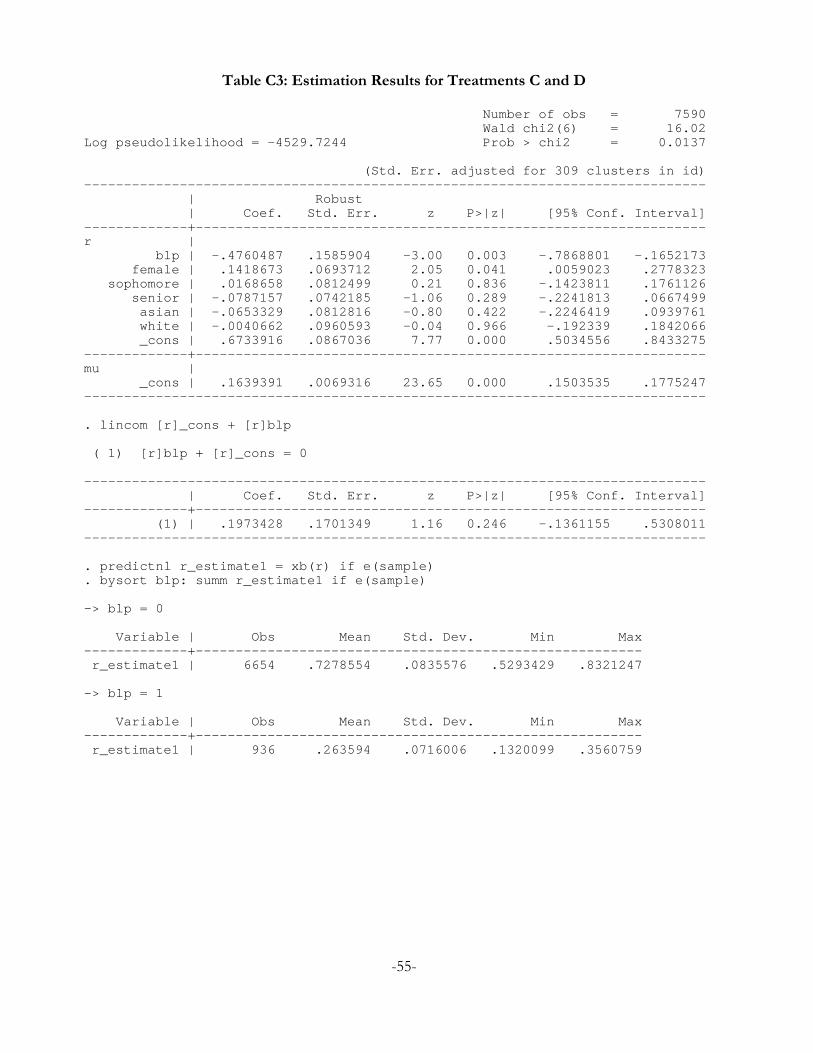
Table C3: Estimation Results for Treatments C and D

Number of obs = 7590 Wald chi2(6) = 16.02Log pseudolikelihood = -4529.7244 Prob > chi2 = 0.0137

(Std. Err. adjusted for 309 clusters in id)------------------------------------------------------------------------------ | Robust | Coef. Std. Err. z P>|z| [95% Conf. Interval]-------------+----------------------------------------------------------------r | blp | -.4760487 .1585904 -3.00 0.003 -.7868801 -.1652173 female | .1418673 .0693712 2.05 0.041 .0059023 .2778323 sophomore | .0168658 .0812499 0.21 0.836 -.1423811 .1761126 senior | -.0787157 .0742185 -1.06 0.289 -.2241813 .0667499 asian | -.0653329 .0812816 -0.80 0.422 -.2246419 .0939761 white | -.0040662 .0960593 -0.04 0.966 -.192339 .1842066 _cons | .6733916 .0867036 7.77 0.000 .5034556 .8433275-------------+----------------------------------------------------------------mu | _cons | .1639391 .0069316 23.65 0.000 .1503535 .1775247------------------------------------------------------------------------------

. lincom [r]_cons + [r]blp

( 1) [r]blp + [r]_cons = 0

------------------------------------------------------------------------------ | Coef. Std. Err. z P>|z| [95% Conf. Interval]-------------+---------------------------------------------------------------- (1) | .1973428 .1701349 1.16 0.246 -.1361155 .5308011------------------------------------------------------------------------------

. predictnl r_estimate1 = xb(r) if e(sample)

. bysort blp: summ r_estimate1 if e(sample)

-> blp = 0

Variable | Obs Mean Std. Dev. Min Max-------------+-------------------------------------------------------- r_estimate1 | 6654 .7278554 .0835576 .5293429 .8321247

-> blp = 1

Variable | Obs Mean Std. Dev. Min Max-------------+-------------------------------------------------------- r_estimate1 | 936 .263594 .0716006 .1320099 .3560759

-55-