Embed Size (px)
Citation preview
Annales Geophysicae, 23, 1735–1746, 2005SRef-ID: 1432-0576/ag/2005-23-1735© European Geosciences Union 2005
AnnalesGeophysicae
Induction effects on ionospheric electric and magnetic fields
H. Vanhamaki, A. Viljanen, and O. Amm
Finnish Meteorological Institute, Space Research Unit, P.O.Box 503, FI-00101 Helsinki, Finland
Received: 15 November 2004 – Revised: 31 March 2005 – Accepted: 14 April 2005 – Published: 28 July 2005
Abstract. Rapid changes in the ionospheric current sys-tem give rise to induction currents in the conducting groundthat can significantly contribute to magnetic and especiallyelectric fields at the Earth’s surface. Previous studies haveconcentrated on the surface fields, as they are important in,for example, interpreting magnetometer measurements or inthe studies of the Earth’s conductivity structure. In thispaper we investigate the effects of induction fields at theionospheric altitudes for several realistic ionospheric currentmodels (Westward Travelling Surge,-band, Giant Pulsa-tion). Our main conclusions are: 1) The secondary electricfield caused by the Earth’s induction is relatively small atthe ionospheric altitude, at most 0.4 mV/m or a few percentof the total electric field; 2) The primary induced field dueto ionospheric self-induction is locally important,∼ a fewmV/m, in some “hot spots”, where the ionospheric conduc-tivity is high and the total electric field is low. However, ourapproximate calculation only gives an upper estimate for theprimary induced electric field; 3) The secondary magneticfield caused by the Earth’s induction may significantly affectthe magnetic measurements of low orbiting satellites. Thesecondary contribution from the Earth’s currents is largest inthe vertical component of the magnetic field, where it maybe around 50% of the field caused by ionospheric currents.
Keywords. Geomagnetism and paleomagnetism (geomag-netic induction) – Ionosphere (electric fields and currents)
1 Introduction
In this paper we investigate the effects of induction on iono-spheric electric and magnetic fields. Ionospheric currentsmay change very rapidly in response to magnetospheric driv-ing, especially during magnetic storms and substorms. Asthe ionospheric current system and the accompanying pri-mary magnetic field vary, a primary induced electric field isproduced in accordance with Faraday’s law of induction. Inaddition, if the Earth’s conductivity is nonzero, the induced
Correspondence to:H. Vanhamaki([email protected])
electric field drives currents in the Earth and these currents,in turn, produce the secondary electric and magnetic fields.
In the majority of studies where ionospheric processes areinvestigated, the ionospheric electric field is assumed to becurl-free, i.e. induction effects are ignored (e.g. Untiedt andBaumjohann, 1993). However, in some cases, for example,Alfv en wave reflection (Yoshikawa and Itonaga, 1996, 2000;Buchert, 1998), inductive effects may have a significant role.The inductive field is, of course, important in studies of in-duction in the Earth. In these studies the main attention isgiven to magnetic and/or electric fields at the Earth’s surface,as these are needed, for example, when calculating geomag-netically induced currents (GIC) in man-made conductor sys-tems (electric grids, pipelines, etc.; see, for example, Vilja-nen et al., 1999, 2004 and references therein) or in studies ofthe conductivity structure of the crust and upper mantle (e.g.Olsen, 1998, 1999; Constable and Constable, 2004).
In this paper our purpose is to investigate the relative mag-nitudes of the primary (Ep) and secondary (Es) inductivefields with respect to the driving electric field (E0) in differ-ent realistic situations. We also investigate the magnitude ofthe secondary magnetic field (Bs) produced by the Earth’scurrents as compared to the primary field (Bp) produced bythe ionospheric currents at different altitudes and discuss theimplications to satellite measurements. This is the first timethat these effects are studied using realistic time-dependentthree-dimensional models for high latitude ionospheric cur-rent systems.
Our nomenclature, already used above, concerning the dif-ferent fields is as follows. The driving electric fieldE0
gives rise to the current densityJ 0=6·E0, where6 is theionospheric conductance tensor. The models of ionospheric
current systems that we use consist ofE0, 6 andJ 0. E0is assumed to be caused by magnetospheric processes andmapped along the magnetic field lines to the ionosphere. Inall the models we use∇×E0=0, i.e. the input electric fielddoes not include any induction effects. The currentsJ 0 pro-duce the primary magnetic fieldBp and, if there is timedependence, the primary induced electric fieldEp, so that∇×Ep
=−∂tBp. If the Earth’s conductivity is nonzero, in-
duced currents flowing in the Earth cause the secondary elec-tric and magnetic fields, which also satisfy∇×Es
=−∂tBs .

1736 H. Vanhamaki et al.: Ionospheric induction effects
The total electric and magnetic fields in the ionosphere areE0+Ep
+Es andBp+Bs , respectively.
We assume the ionosphere to be a thin horizontal sheet110 km above the ground, so that effects of spherical geome-try and vertical variations within the ionosphere are ignored.Furthermore, the Earth’s conductivity structure is assumed tobe one-dimensional, so that the Earth consists of horizontallayers and each layer has a constant conductivityσ , permit-tivity ε and permeabilityµ(=µ0).
We represent the ionospheric current systems as superpo-sitions of Cartesian Elementary Current Systems (CECS).Amm (1997) introduced two different CECS, one being curl-free and the other divergence-free. Any continuously deriv-able two-dimensional vector field can be presented as a sumof an infinite number of these elementary systems. The use ofCECS simplifies the calculations, as analytical expressionsfor the electric and magnetic fields of these current systemsexist.
The inductive response of the Earth is calculated using thecomplex image method (CIM) introduced to geophysical ap-plications by Thomson and Weaver (1975). In CIM the lay-ered Earth is replaced by a perfect conductor at a complexdepth, and the secondary electric and magnetic fields pro-duced by the currents flowing in the Earth can be calculatedby the standard image principle. The depth of the perfectconductorp can be calculated from the plane wave surfaceimpedanceZ(ω) as
p=Z(ω)
iωµ0, (1)
whereω is the angular frequency. Once the thicknesses andconductivities of the Earth layers are specified, the surfaceimpedanceZ(ω) can be calculated by using a recursion for-mula given, for example, by Wait (1981, pp. 52–53).
In most cases CIM gives very good approximations to theexact solutions and we believe it to be completely adequatefor our purposes (see Thomson and Weaver, 1975; Botelerand Pirjola, 1998; Pirjola and Viljanen, 1998; Shepherd andShubitidze, 2003, for discussions of accuracy). The neglec-tion of horizontal variations in the Earth’s conductivity maynot always be a valid approximation, as large horizontal con-ductivity gradients exists, for example, between well con-ducting oceans and more resistive inland areas. However,in this study we are interested in the order of magnitude ofthe secondary fields and for this purpose the layered Earthassumption is adequate.
While the response of the conducting ground to externalsources is described with a very good accuracy by CIM,our treatment of the ionospheric induction is more approx-imate. We calculate the primary and secondary induced elec-tric fieldsEp andEs in the ionosphere using Eqs. (4, 6, 9 and11). These equations give the fields in a vacuum, i.e. they donot take into account the response of the ionospheric plasma.In reality, the induced electric fields would drive currents inthe ionosphere and these currents would cause their own sec-ond order induction phenomena, and so on. In this sense ourtreatment corresponds to terminating this iterative loop in the
zeroth order. The higher order corrections would obviouslydecrease the total induced electric field, in accordance withLenz’s law, and therefore we obtain upper estimates for theinduction effects. The induced currents in the ionosphere andassociated field-aligned currents would also create their ownmagnetic fields both below and above the ionosphere, but wealso neglect these effects.
The paper is organized so that in Sect. 2 we give theexpression for the primary and secondary electromagneticfields of the curl- and divergence-free elementary systems.In Sect. 3 we apply the combined CECS and CIM to dif-ferent ionospheric model systems and compare the primaryand secondary induced electric fields with the driving elec-tric field of the models. Section 4 deals with the effect ofEarth induction on satellite measurements of magnetic fieldvariations at heights of a few hundred km.
2 Fields of elementary systems
We use a coordinate system in whichx is northward,y iseastward andz is vertically down. The Earth’s surface isthe xy-plane and ionospheric currents are assumed to flowat heighth (i.e. z=−h). A more detailed derivation of theexpressions for the primary and secondary electromagneticfields of the divergence- and curl-free CECS is given in theAppendix; here we just give the final results.
The current density of the divergence-free CECS (Fig. 1),in cylindrical coordinates centered on the pole of the CECS,is given by Amm (1997) as (misprint in his formula correctedhere)
jdf=
I0
2πρδ(z + h) eφ . (2)
The magnitude of the elementary system is denoted byI0,andδ is the Dirac delta function. This current system givesrise to a primary magnetic field
Bdf,p=
µ0I0
4πρ
([1−
|z+h|√ρ2+(z+h)2
]sign(z+h)eρ+
+ρ√
ρ2+(z+h)2ez
)(3)
and a primary induced electric field (harmonic time depen-denceeiωt with the angular frequencyω is assumed)
Edf,p=
−iωµ0I0
4πρ
(√ρ2+(z+h)2−|z+h|
)eφ . (4)
For a layered Earth model, the secondary fields producedby induced currents in the Earth can be calculated by usingCIM. In this case the secondary fields of a divergence-freeelementary system above the ground (z≤0) are
Bdf,s=
µ0I0
4πρ
([1−
h+2p−z√ρ2+(h+2p−z)2
]eρ−
H. Vanhamaki et al.: Ionospheric induction effects 1737
Fig. 1. The current density of the curl-free CECS (upper) and thedivergence-free CECS (lower).
−ρ√
ρ2+(h+2p−z)2ez
)(5)
Edf,s=
iωµ0I0
4πρ
(√ρ2+(h+2p−z)2−(h+2p−z)
)eφ . (6)
The depth of the perfect conductorp is given by Eq. (1).Similarly, for the curl-free CECS the current density is
j cf=
I0
2πρδ(z+h)eρ+I0δ(x)δ(y)U(−z−h)ez, (7)
whereU is the Heaviside unit step function. The primarymagnetic and electric fields are
Bcf,p=
−µ0I0
2πρU(−z−h)eφ (8)
Ecf,p=
−iωµ0I0
4πρ
([√ρ2+(z+h)2−|z+h|
]eρ −
−ρ log(k0
√ρ2+(z+h)2+k0(z+h))ez
). (9)
In the last equationk0=ω/c is the vacuum wave number. Inpractise the z-component of the electric field is not important,because it (in good approximation) cancels due to the veryhigh field-aligned conductivity in the ionosphere.
For a curl-free CECS CIM cannot be applied, but the sec-ondary fields can be calculated in a different manner, as ex-plained in the Appendix. For all geophysically reasonable
−600 −400 −200 0 200 400 600−400
−200
0
200
400
X, k
m
WTS, E0, max=30.9 mV/m
−600 −400 −200 0 200 400 600−400
−200
0
200
400
Y, km
X, k
m
WTS, J0, max=756 A/km
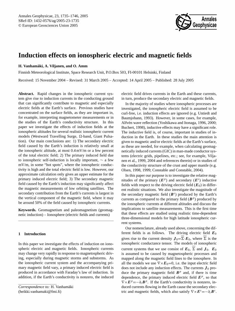
Fig. 2. The driving electric field and associated currents of the WTSmodel.
frequencies and conductivities the results can be approxi-mated with negligible errors as
Bcf,s=0 (10)
Ecf,s=
iωµ0I0
4πρ
([√ρ2+(h − z)2−(h−z)
]eρ+
+
[log(k0
√ρ2+(h−z)2+k0(z−h))
]ez
). (11)
Concerning the horizontal electric field, the Earth behaves asa perfect conductor, so that the horizontal part of the primaryand secondary electric fields produced by curl-free CECS ex-actly cancel at the Earth’s surface.
3 Induced electric fields of different model systems
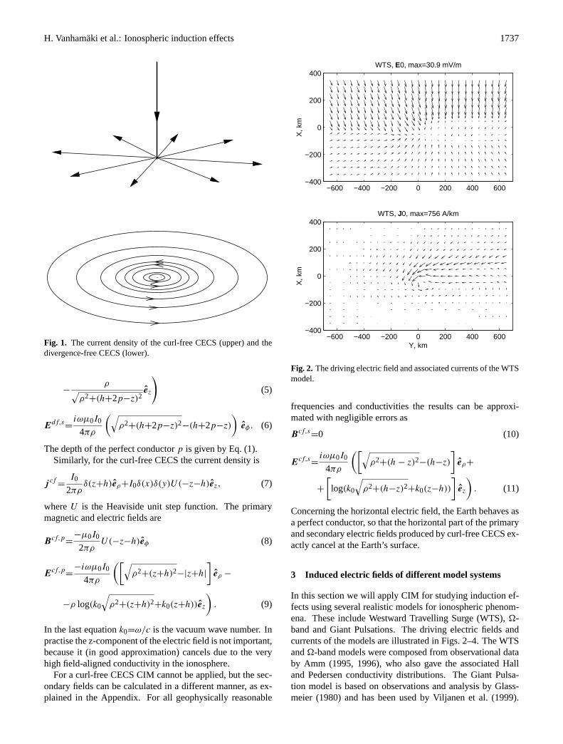
In this section we will apply CIM for studying induction ef-fects using several realistic models for ionospheric phenom-ena. These include Westward Travelling Surge (WTS),-band and Giant Pulsations. The driving electric fields andcurrents of the models are illustrated in Figs. 2–4. The WTSand-band models were composed from observational databy Amm (1995, 1996), who also gave the associated Halland Pedersen conductivity distributions. The Giant Pulsa-tion model is based on observations and analysis by Glass-meier (1980) and has been used by Viljanen et al. (1999).
1738 H. Vanhamaki et al.: Ionospheric induction effects
−200 0 200 400 600−400
−200
0
200
400
X,k
mΩ−band, E0, max=187 mV/m
−200 0 200 400 600−400
−200
0
200
400
Y, km
X, k
m
Ω−band, J0, max=2930 A/km
Fig. 3. The driving electric field and associated currents of the-band model.
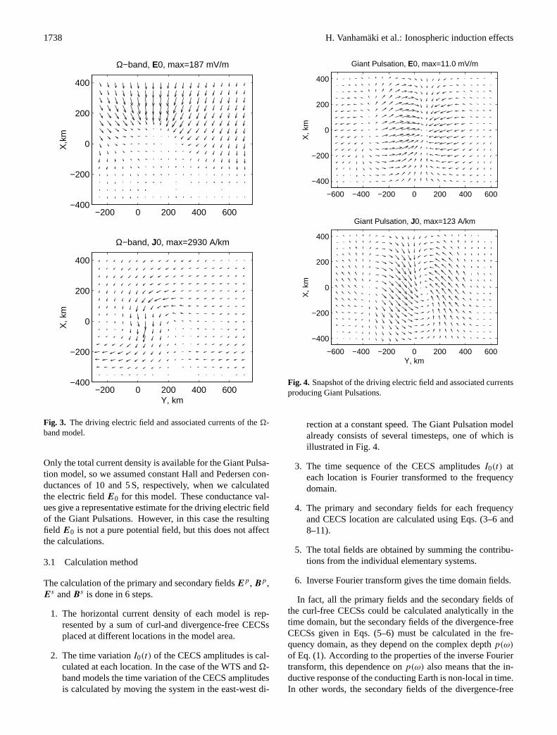
Only the total current density is available for the Giant Pulsa-tion model, so we assumed constant Hall and Pedersen con-ductances of 10 and 5 S, respectively, when we calculatedthe electric fieldE0 for this model. These conductance val-ues give a representative estimate for the driving electric fieldof the Giant Pulsations. However, in this case the resultingfield E0 is not a pure potential field, but this does not affectthe calculations.
3.1 Calculation method
The calculation of the primary and secondary fieldsEp, Bp,Es andBs is done in 6 steps.
1. The horizontal current density of each model is rep-resented by a sum of curl-and divergence-free CECSsplaced at different locations in the model area.
2. The time variationI0(t) of the CECS amplitudes is cal-culated at each location. In the case of the WTS and-band models the time variation of the CECS amplitudesis calculated by moving the system in the east-west di-
−600 −400 −200 0 200 400 600
−400
−200
0
200
400
Giant Pulsation, E0, max=11.0 mV/m
X, k
m
−600 −400 −200 0 200 400 600
−400
−200
0
200
400
Giant Pulsation, J0, max=123 A/km
Y, km
X, k
m
Fig. 4. Snapshot of the driving electric field and associated currentsproducing Giant Pulsations.
rection at a constant speed. The Giant Pulsation modelalready consists of several timesteps, one of which isillustrated in Fig. 4.
3. The time sequence of the CECS amplitudesI0(t) ateach location is Fourier transformed to the frequencydomain.
4. The primary and secondary fields for each frequencyand CECS location are calculated using Eqs. (3–6 and8–11).
5. The total fields are obtained by summing the contribu-tions from the individual elementary systems.
6. Inverse Fourier transform gives the time domain fields.
In fact, all the primary fields and the secondary fields ofthe curl-free CECSs could be calculated analytically in thetime domain, but the secondary fields of the divergence-freeCECSs given in Eqs. (5–6) must be calculated in the fre-quency domain, as they depend on the complex depthp(ω)
of Eq. (1). According to the properties of the inverse Fouriertransform, this dependence onp(ω) also means that the in-ductive response of the conducting Earth is non-local in time.In other words, the secondary fields of the divergence-free

H. Vanhamaki et al.: Ionospheric induction effects 1739
%
0
5
10
15
20
25
−500 0 500
−200
0
200
Y, km
|Ep+Es|/|E0|, max=94.1%, mean=2.0%
−500 0 500−400
−200
0
200
400Es, max=0.32mV/m
−500 0 500−400
−200
0
200
400
X, k
m
Ep, max=2.12 mV/m
−500 0 500−400
−200
0
200
400Jind, max=133 A/km
Y, km
X, k
m
Fig. 5. Upper row: primary (left) and secondary (right) induced electric fields of the WTS model, note the different scales of the plots. Lowerrow: induced currents, i.e. currents driven by induced electric fields (left) and the ratio (primary+secondary induced electric field)/(drivingelectric field) (right). The color scale is limited to 25% while the maximum ratio is 94%.
CECSs at timet are not determined just from the amplitudesI0(t) at that same moment, but the fields are affected by thewhole previous time development ofI0(t
′), t ′≤t .The primary magnetic fieldBp describes the static field
produced by the ionospheric currents and therefore it doesnot depend on the velocity of the current system or its oscil-lation frequency. The primary electric fieldEp is causedby the time variations of the currents and according toEqs. (4 and 9) the dependence onω (and hence also on thevelocity) is linear. The secondary fields of the divergence-free CECSs in Eqs. (5–6) depend on the complex depthp(ω)
and therefore the detailed relationship between the secondaryfields, the Earth’s conductivity structure and the oscillationtime of the Giant Pulsation or velocity of the WTS and-band models is complicated. However, it is clear that rapidtime variations and large Earth conductivity result in largerinduced currents within the Earth and also largerBs andEs
above the Earth.
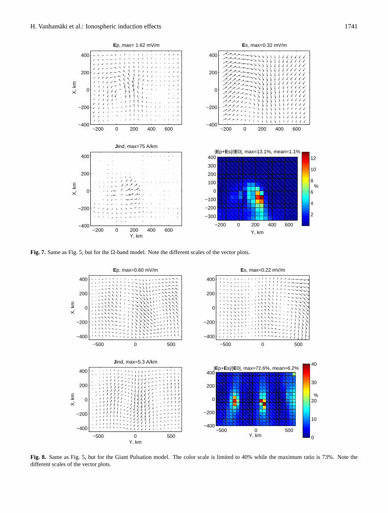
3.2 Results
Figures 5-8 show the resulting primary and secondaryfields for the different models, together with comparison|Ep
+Es|/|E0| against the driving electric field. Also, the
induced ionospheric currentsJ ind driven by Ep+Es are
plotted. These currents were ignored in our calculations, socomparison ofJ ind againstJ 0 for each model system givesan estimate for the magnitude of correction terms these in-duced currents would produce. In these calculations we useda highly conducting “ocean” model in which the layer thick-nesses and resistivities are 3, 147,∞ km (lowest layer issemi-infinite) and 0.25, 100, 1m, respectively. All the lay-ers are assumed to haveµ=µ0 andε=5ε0 (the exact value ofε is not important, as it appears only in the displacement cur-rent term that is negligible in the low frequency limit). TheWTS system moves at a velocity of 10 km/s westward andthe-band at 2 km/s eastward. These values are in the upperrange of realistic speeds (e.g. Paschmann et al., 2002, Chap-ter 6). The oscillation time of the Giant Pulsation is about100 s.
It should be remembered that we calculateEp andEs asif the ionosphere were a vacuum, i.e. we ignore the currentsdriven by the induced electric fields. For this reason the re-sults in Figs. 5–8 should be considered as upper limits for theinduced electric fields, since the response of the ionosphericplasma should decrease the fields.
From Figs. 5, 7 and 8 it is obvious that in most cases the in-ductive electric fields are much smaller than the correspond-ing driving electric fields and that the secondary contribu-tion to inductive fields is small compared to the primary part.
1740 H. Vanhamaki et al.: Ionospheric induction effects
−400
−200
0
200
400
X, k
m
J0, Pedersen, max=278 A/km
−400
−200
0
200
400Jind, Pedersen, max=35 A/km
−400
−200
0
200
400
X, k
m
J0, Hall, max=721 A/km
−400
−200
0
200
400Jind, Hall, max=131 A/km
−400
−200
0
200
400
X, k
m
J0, curl−free, max=331 A/km
−400
−200
0
200
400Jind, curl−free, max=91 A/km
−500 0 500−400
−200
0
200
400
Y, km
X, k
m
J0, div−free, max=603 A/km
−500 0 500−400
−200
0
200
400Jind, div−free, max=78 A/km
Y, km
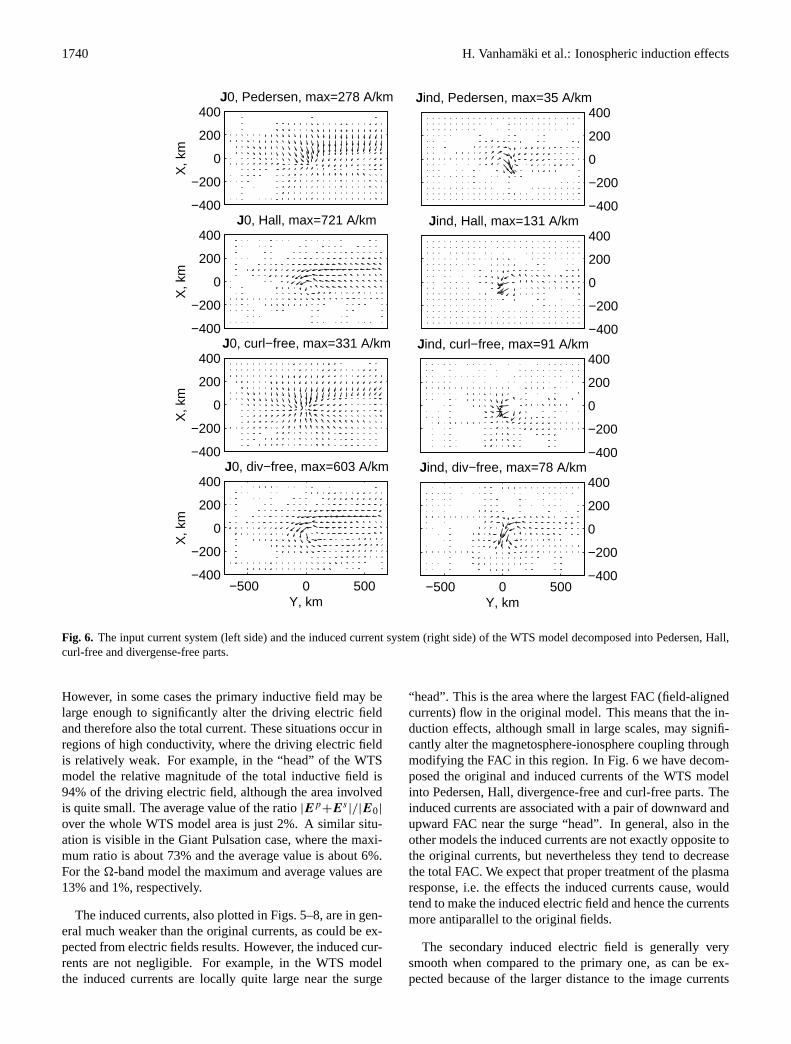
Fig. 6. The input current system (left side) and the induced current system (right side) of the WTS model decomposed into Pedersen, Hall,curl-free and divergense-free parts.
However, in some cases the primary inductive field may belarge enough to significantly alter the driving electric fieldand therefore also the total current. These situations occur inregions of high conductivity, where the driving electric fieldis relatively weak. For example, in the “head” of the WTSmodel the relative magnitude of the total inductive field is94% of the driving electric field, although the area involvedis quite small. The average value of the ratio|Ep
+Es|/|E0|
over the whole WTS model area is just 2%. A similar situ-ation is visible in the Giant Pulsation case, where the maxi-mum ratio is about 73% and the average value is about 6%.For the-band model the maximum and average values are13% and 1%, respectively.
The induced currents, also plotted in Figs. 5–8, are in gen-eral much weaker than the original currents, as could be ex-pected from electric fields results. However, the induced cur-rents are not negligible. For example, in the WTS modelthe induced currents are locally quite large near the surge
“head”. This is the area where the largest FAC (field-alignedcurrents) flow in the original model. This means that the in-duction effects, although small in large scales, may signifi-cantly alter the magnetosphere-ionosphere coupling throughmodifying the FAC in this region. In Fig. 6 we have decom-posed the original and induced currents of the WTS modelinto Pedersen, Hall, divergence-free and curl-free parts. Theinduced currents are associated with a pair of downward andupward FAC near the surge “head”. In general, also in theother models the induced currents are not exactly opposite tothe original currents, but nevertheless they tend to decreasethe total FAC. We expect that proper treatment of the plasmaresponse, i.e. the effects the induced currents cause, wouldtend to make the induced electric field and hence the currentsmore antiparallel to the original fields.
The secondary induced electric field is generally verysmooth when compared to the primary one, as can be ex-pected because of the larger distance to the image currents
H. Vanhamaki et al.: Ionospheric induction effects 1741
%
2
4
6
8
10
12
−200 0 200 400 600
−300
−200
−100
0
100
200
300
400
Y, km
|Ep+Es|/|E0|, max=13.1%, mean=1.1%
−200 0 200 400 600−400
−200
0
200
400
Ep, max= 1.62 mV/m
X, k
m
−200 0 200 400 600−400
−200
0
200
400
X, k
m
Y, km
Jind, max=75 A/km
−200 0 200 400 600−400
−200
0
200
400
Es, max=0.32 mV/m
Fig. 7. Same as Fig. 5, but for the-band model. Note the different scales of the vector plots.
−500 0 500
−400
−200
0
200
400
X, k
m
Ep, max=0.60 mV/m
−500 0 500
−400
−200
0
200
400
Es, max=0.22 mV/m
−500 0 500
−400
−200
0
200
400
Y, km
X, k
m
Jind, max=5.3 A/km
%
0
10
20
30
40
−500 0 500−400
−200
0
200
400
Y, km
|Ep+Es|/|E0|, max=72.6%, mean=6.2%
Fig. 8. Same as Fig. 5, but for the Giant Pulsation model. The color scale is limited to 40% while the maximum ratio is 73%. Note thedifferent scales of the vector plots.
1742 H. Vanhamaki et al.: Ionospheric induction effects
0 100 200 300 400 500−1000
−500
0
500
1000
1500X−comp
nT
Bp+BsBpBs
0 100 200 300 400 500−600
−400
−200
0
200
400Y−comp
Bp+BsBpBs
0 100 200 300 400 500−1000
−800
−600
−400
−200
0
200
400
Z−comp
Height, km
nT
Bp+BsBpBs
0 100 200 300 400 5000
400
800
1200
1600|B|
Height, km
Bp+BsBpBs
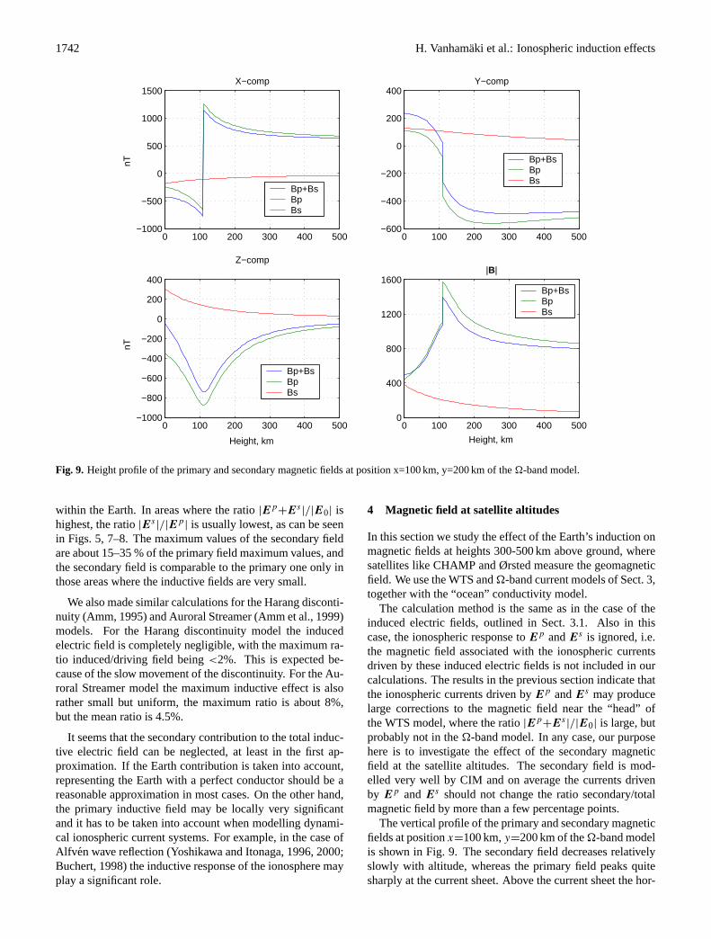
Fig. 9. Height profile of the primary and secondary magnetic fields at position x=100 km, y=200 km of the-band model.
within the Earth. In areas where the ratio|Ep+Es
|/|E0| ishighest, the ratio|Es
|/|Ep| is usually lowest, as can be seen
in Figs. 5, 7–8. The maximum values of the secondary fieldare about 15–35 % of the primary field maximum values, andthe secondary field is comparable to the primary one only inthose areas where the inductive fields are very small.
We also made similar calculations for the Harang disconti-nuity (Amm, 1995) and Auroral Streamer (Amm et al., 1999)models. For the Harang discontinuity model the inducedelectric field is completely negligible, with the maximum ra-tio induced/driving field being<2%. This is expected be-cause of the slow movement of the discontinuity. For the Au-roral Streamer model the maximum inductive effect is alsorather small but uniform, the maximum ratio is about 8%,but the mean ratio is 4.5%.
It seems that the secondary contribution to the total induc-tive electric field can be neglected, at least in the first ap-proximation. If the Earth contribution is taken into account,representing the Earth with a perfect conductor should be areasonable approximation in most cases. On the other hand,the primary inductive field may be locally very significantand it has to be taken into account when modelling dynami-cal ionospheric current systems. For example, in the case ofAlfv en wave reflection (Yoshikawa and Itonaga, 1996, 2000;Buchert, 1998) the inductive response of the ionosphere mayplay a significant role.
4 Magnetic field at satellite altitudes
In this section we study the effect of the Earth’s induction onmagnetic fields at heights 300-500 km above ground, wheresatellites like CHAMP and Ørsted measure the geomagneticfield. We use the WTS and-band current models of Sect. 3,together with the “ocean” conductivity model.
The calculation method is the same as in the case of theinduced electric fields, outlined in Sect. 3.1. Also in thiscase, the ionospheric response toEp andEs is ignored, i.e.the magnetic field associated with the ionospheric currentsdriven by these induced electric fields is not included in ourcalculations. The results in the previous section indicate thatthe ionospheric currents driven byEp andEs may producelarge corrections to the magnetic field near the “head” ofthe WTS model, where the ratio|Ep
+Es|/|E0| is large, but
probably not in the-band model. In any case, our purposehere is to investigate the effect of the secondary magneticfield at the satellite altitudes. The secondary field is mod-elled very well by CIM and on average the currents drivenby Ep andEs should not change the ratio secondary/totalmagnetic field by more than a few percentage points.
The vertical profile of the primary and secondary magneticfields at positionx=100 km,y=200 km of the-band modelis shown in Fig. 9. The secondary field decreases relativelyslowly with altitude, whereas the primary field peaks quitesharply at the current sheet. Above the current sheet the hor-
H. Vanhamaki et al.: Ionospheric induction effects 1743
0 100 200 300 400 5000
20
40
60
80
100Ω−band, x=100 km, y=200 km
%
horizontalvertical
0 100 200 300 400 5000
20
40
60
80
100Ω−band, x=−200 km, y=200 km
horizontalvertical
0 100 200 300 400 5000
20
40
60
80
100WTS, x=0 km, y=0 km
Height, km
%
horizontalvertical
0 100 200 300 400 5000
20
40
60
80
100WTS, x=0 km, y=400 km
Height, km
horizontalvertical
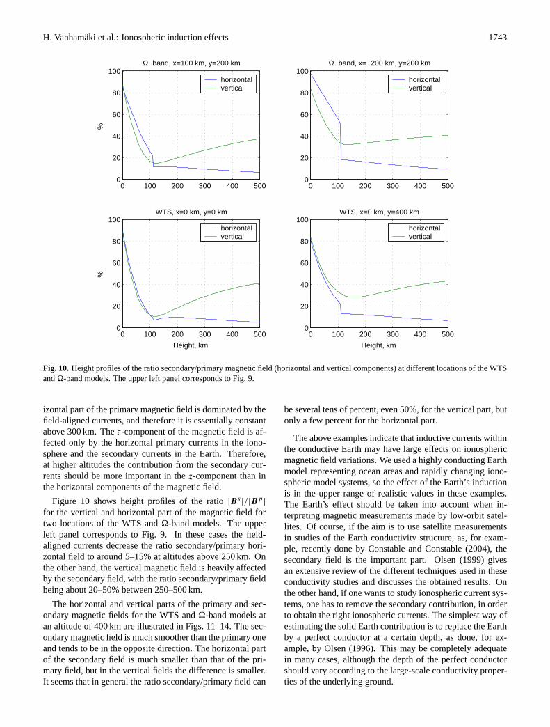
Fig. 10.Height profiles of the ratio secondary/primary magnetic field (horizontal and vertical components) at different locations of the WTSand-band models. The upper left panel corresponds to Fig. 9.
izontal part of the primary magnetic field is dominated by thefield-aligned currents, and therefore it is essentially constantabove 300 km. Thez-component of the magnetic field is af-fected only by the horizontal primary currents in the iono-sphere and the secondary currents in the Earth. Therefore,at higher altitudes the contribution from the secondary cur-rents should be more important in thez-component than inthe horizontal components of the magnetic field.
Figure 10 shows height profiles of the ratio|Bs|/|Bp
|
for the vertical and horizontal part of the magnetic field fortwo locations of the WTS and-band models. The upperleft panel corresponds to Fig. 9. In these cases the field-aligned currents decrease the ratio secondary/primary hori-zontal field to around 5–15% at altitudes above 250 km. Onthe other hand, the vertical magnetic field is heavily affectedby the secondary field, with the ratio secondary/primary fieldbeing about 20–50% between 250–500 km.
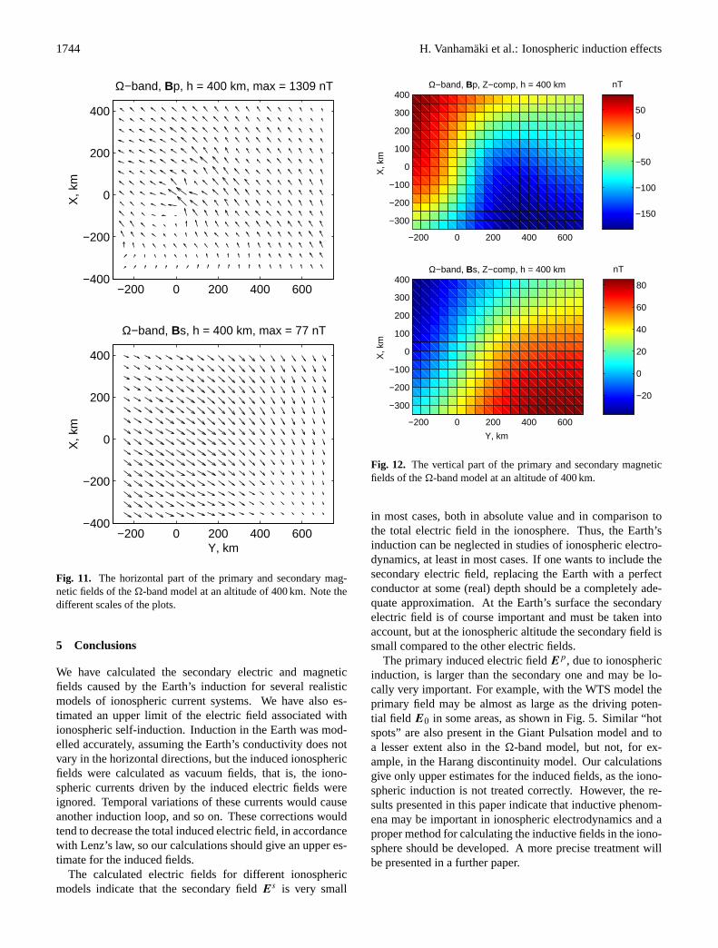
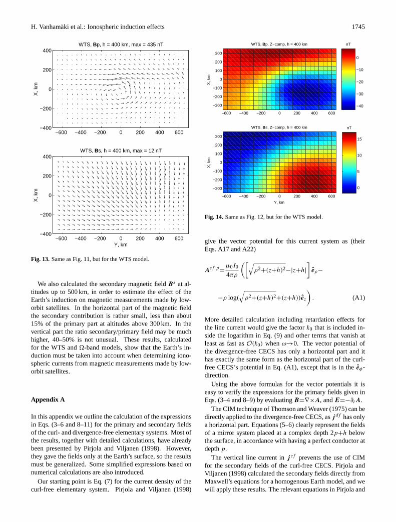
The horizontal and vertical parts of the primary and sec-ondary magnetic fields for the WTS and-band models atan altitude of 400 km are illustrated in Figs. 11–14. The sec-ondary magnetic field is much smoother than the primary oneand tends to be in the opposite direction. The horizontal partof the secondary field is much smaller than that of the pri-mary field, but in the vertical fields the difference is smaller.It seems that in general the ratio secondary/primary field can
be several tens of percent, even 50%, for the vertical part, butonly a few percent for the horizontal part.
The above examples indicate that inductive currents withinthe conductive Earth may have large effects on ionosphericmagnetic field variations. We used a highly conducting Earthmodel representing ocean areas and rapidly changing iono-spheric model systems, so the effect of the Earth’s inductionis in the upper range of realistic values in these examples.The Earth’s effect should be taken into account when in-terpreting magnetic measurements made by low-orbit satel-lites. Of course, if the aim is to use satellite measurementsin studies of the Earth conductivity structure, as, for exam-ple, recently done by Constable and Constable (2004), thesecondary field is the important part. Olsen (1999) givesan extensive review of the different techniques used in theseconductivity studies and discusses the obtained results. Onthe other hand, if one wants to study ionospheric current sys-tems, one has to remove the secondary contribution, in orderto obtain the right ionospheric currents. The simplest way ofestimating the solid Earth contribution is to replace the Earthby a perfect conductor at a certain depth, as done, for ex-ample, by Olsen (1996). This may be completely adequatein many cases, although the depth of the perfect conductorshould vary according to the large-scale conductivity proper-ties of the underlying ground.
1744 H. Vanhamaki et al.: Ionospheric induction effects
−200 0 200 400 600−400
−200
0
200
400
Ω−band, Bp, h = 400 km, max = 1309 nTX
, km
−200 0 200 400 600−400
−200
0
200
400
Ω−band, Bs, h = 400 km, max = 77 nT
X, k
m
Y, km
Fig. 11. The horizontal part of the primary and secondary mag-netic fields of the-band model at an altitude of 400 km. Note thedifferent scales of the plots.
5 Conclusions
We have calculated the secondary electric and magneticfields caused by the Earth’s induction for several realisticmodels of ionospheric current systems. We have also es-timated an upper limit of the electric field associated withionospheric self-induction. Induction in the Earth was mod-elled accurately, assuming the Earth’s conductivity does notvary in the horizontal directions, but the induced ionosphericfields were calculated as vacuum fields, that is, the iono-spheric currents driven by the induced electric fields wereignored. Temporal variations of these currents would causeanother induction loop, and so on. These corrections wouldtend to decrease the total induced electric field, in accordancewith Lenz’s law, so our calculations should give an upper es-timate for the induced fields.
The calculated electric fields for different ionosphericmodels indicate that the secondary fieldEs is very small
nT
−150
−100
−50
0
50
−200 0 200 400 600
−300
−200
−100
0
100
200
300
400
X, k
m
Ω−band, Bp, Z−comp, h = 400 km
nT
−20
0
20
40
60
80
−200 0 200 400 600
−300
−200
−100
0
100
200
300
400
Y, km
X, k
m
Ω−band, Bs, Z−comp, h = 400 km
Fig. 12. The vertical part of the primary and secondary magneticfields of the-band model at an altitude of 400 km.
in most cases, both in absolute value and in comparison tothe total electric field in the ionosphere. Thus, the Earth’sinduction can be neglected in studies of ionospheric electro-dynamics, at least in most cases. If one wants to include thesecondary electric field, replacing the Earth with a perfectconductor at some (real) depth should be a completely ade-quate approximation. At the Earth’s surface the secondaryelectric field is of course important and must be taken intoaccount, but at the ionospheric altitude the secondary field issmall compared to the other electric fields.
The primary induced electric fieldEp, due to ionosphericinduction, is larger than the secondary one and may be lo-cally very important. For example, with the WTS model theprimary field may be almost as large as the driving poten-tial field E0 in some areas, as shown in Fig. 5. Similar “hotspots” are also present in the Giant Pulsation model and toa lesser extent also in the-band model, but not, for ex-ample, in the Harang discontinuity model. Our calculationsgive only upper estimates for the induced fields, as the iono-spheric induction is not treated correctly. However, the re-sults presented in this paper indicate that inductive phenom-ena may be important in ionospheric electrodynamics and aproper method for calculating the inductive fields in the iono-sphere should be developed. A more precise treatment willbe presented in a further paper.
H. Vanhamaki et al.: Ionospheric induction effects 1745
−600 −400 −200 0 200 400 600−400
−200
0
200
400WTS, Bp, h = 400 km, max = 435 nT
X, k
m
−600 −400 −200 0 200 400 600−400
−200
0
200
400WTS, Bs, h = 400 km, max = 12 nT
X, k
m
Y, km
Fig. 13. Same as Fig. 11, but for the WTS model.
We also calculated the secondary magnetic fieldBs at al-titudes up to 500 km, in order to estimate the effect of theEarth’s induction on magnetic measurements made by low-orbit satellites. In the horizontal part of the magnetic fieldthe secondary contribution is rather small, less than about15% of the primary part at altitudes above 300 km. In thevertical part the ratio secondary/primary field may be muchhigher, 40–50% is not unusual. These results, calculatedfor the WTS and-band models, show that the Earth’s in-duction must be taken into account when determining iono-spheric currents from magnetic measurements made by low-orbit satellites.
Appendix A
In this appendix we outline the calculation of the expressionsin Eqs. (3–6 and 8–11) for the primary and secondary fieldsof the curl- and divergence-free elementary systems. Most ofthe results, together with detailed calculations, have alreadybeen presented by Pirjola and Viljanen (1998). However,they gave the fields only at the Earth’s surface, so the resultsmust be generalized. Some simplified expressions based onnumerical calculations are also introduced.
Our starting point is Eq. (7) for the current density of thecurl-free elementary system. Pirjola and Viljanen (1998)
nT
−40
−30
−20
−10
0
−600 −400 −200 0 200 400 600
−300
−200
−100
0
100
200
300
X, k
m
WTS, Bp, Z−comp, h = 400 km
nT
0
5
10
15
−600 −400 −200 0 200 400 600
−300
−200
−100
0
100
200
300
Y, kmX
, km
WTS, Bs, Z−comp, h = 400 km
Fig. 14. Same as Fig. 12, but for the WTS model.
give the vector potential for this current system as (theirEqs. A17 and A22)
Acf,p=
µ0I0
4πρ
([√ρ2+(z+h)2−|z+h|
]eρ−
−ρ log(
√ρ2+(z+h)2+(z+h))ez
). (A1)
More detailed calculation including retardation effects forthe line current would give the factork0 that is included in-side the logarithm in Eq. (9) and other terms that vanish atleast as fast asO(k0) whenω→0. The vector potential ofthe divergence-free CECS has only a horizontal part and ithas exactly the same form as the horizontal part of the curl-free CECS’s potential in Eq. (A1), except that is in theeφ-direction.
Using the above formulas for the vector potentials it iseasy to verify the expressions for the primary fields given inEqs. (3–4 and 8–9) by evaluatingB=∇×A, andE=−∂tA.
The CIM technique of Thomson and Weaver (1975) can bedirectly applied to the divergence-free CECS, asjdf has onlya horizontal part. Equations (5–6) clearly represent the fieldsof a mirror system placed at a complex depth 2p+h belowthe surface, in accordance with having a perfect conductor atdepthp.
The vertical line current inj cf prevents the use of CIMfor the secondary fields of the curl-free CECS. Pirjola andViljanen (1998) calculated the secondary fields directly fromMaxwell’s equations for a homogenous Earth model, and wewill apply these results. The relevant equations in Pirjola and
1746 H. Vanhamaki et al.: Ionospheric induction effects
Viljanen (1998) read (their Eqs. A2, A6, A9, A10, A11 andA29)
Bcf,sφ =
∫∞
0C(b)J1(bρ)eκ0zdb, (A2)
Ecf,sρ =
iω
k20
∫∞
0κ0C(b)J1(bρ)eκ0zdb, (A3)
Ecf,sz =
−iω
k20
∫∞
0bC(b)J0(bρ)eκ0zdb, (A4)
C(b)=µ0I0
4πk2
0k2 e−hb
b(k2κ0+k20κ)
, (A5)
k2=ω2µε−iωµσ,
−π
4≤ arg(k)≤0, (A6)
κ2=b2
−k2,−π
2≤ arg(κ)≤
π
2, (A7)
These expressions are valid in the half spacez≤0. J0 andJ1 are the zeroth and first order Bessel functions, whilek0and κ0 are values ofk and κ in the air, with parametersµ0, ε0, σ=0.
Numerical evaluation of the above expressions for the sec-ondary fields of the curl-free CECS reveals that for all geo-physically reasonable frequencies (ω=10. . . 10−4 s−1) andconductivities (σ=10. . . 10−5(m)−1) they can be approx-imated with the formulas given in Eqs. (10–11). Errors inthese approximations are<0.1%, at least in the distancerangeρ≤500 km, 0≤z≤500 km, where the fields are needed.Pirjola and Viljanen (1998) derived their analytical resultsfor the homogenous conductivity case, but they also per-formed numerical calculations for a layered Earth conductiv-ity model. These calculations confirmed that for a curl-freeCECS the secondary magnetic field vanishes above the Earthand the secondary electric field can be calculated as if theEarth were a perfect conductor. Thus, Eqs. (10–11) can bealso used with layered Earth conductivity models.
Acknowledgements.We thank R. Pirjola (at Finnish MeteorologicalInstitute) for his comments on the manuscript. The work of H. Van-hamaki is supported by the Finnish Graduate School in Astronomyand Space Physics.
Topical Editor M. Lester thanks A. Yoshikawa and E. Woodfieldfor their help in evaluating this paper.
References
Amm, O.: Direct determination of the local ionospheric Hall con-ductance distribution from two-dimensional electric and mag-netic field data: Application of the method using models of typi-cal ionospheric electrodynamic situations, J. Geophys. Res., 100,21 473–21 488, 1995.
Amm, O.: Improved electrodynamic modeling of an omega bandand analysis of its current system, J. Geophys. Res., 101, 2677–2683, 1996.
Amm, O.: Ionospheric elementary current systems in spherical co-ordinates and their application, J. Geomag. Geoelect., 49, 947–955, 1997.
Amm, O., Pajunpaa, A., and Brandstrom, U.: Spatial distributionof conductances, currents, and field-aligned currents associatedwith a north-south auroral structure during a highly disturbedmultiple-substorm period, Ann. Geophys., 17, 1385–1396, 1999,SRef-ID: 1432-0576/ag/1999-17-1385.
Boteler, D. and Pirjola, R.: The complex-image method for calcu-lating the magnetic and electric fields produced at the surface ofthe Earth by the auroral electrojet, Geophys. J. Int., 132, 31–40,1998.
Buchert, S.: Magneto-optical Kerr effect for a dissipative plasma, J.Plasma Physics, 59, 39–55, 1998.
Constable, S. and Constable, C.: Observing geomagnetic induc-tion in magnetic satellite measurements and associated impli-cations for mantle conductivity, Geochem. Geophys. Geosyst.,5Q01006, doi:10.1029/2003GC000634, 2004.
Glassmeier, K.-H.: Magnetometer Array Observations of a GiantPulsation, J. Geophys., 48, 127–138, 1980.
Olsen, N.: A new tool for determining ionospheric currents frommagnetic satellite data, Geophys. Res. Lett., 23, 3635–3638,1996.
Olsen, N.: The electrical conductivity of the mantle beneath Europederived fromC-responces from 3 to 720 h, Geophys. J. Int. 133,298–308, 1998.
Olsen, N.: Induction studies with satellite data, Surveys in Geo-physics, 20, 309–340, 1999.
Paschmann, G., Haaland, S., and Treumann, R.: Auroral PlasmaPhysics, Space Sci. Rev., 103, 1–475, 2002.
Pirjola, R. and Viljanen, A.: Complex image method for calculatingelectric and magnetic fields produced by an auroral electrojet offinite length, Ann. Geophys., 16, 1434–1444, 1998,SRef-ID: 1432-0576/ag/1998-16-1434.
Shepherd, S. and Shubitidze, F.: Method of auxiliary sources forcalculating the magnetic and electric fields induced in a layeredEarth, J. Atmos. Sol.-Terr. Phys., 65, 1151–1160, 2003.
Thomson, D. and Weaver, J.: The Complex Image Approximationfor Induction in a Multilayered Earth, J. Geophys. Res., 80, 123–129, 1975.
Untiedt, J. and Baumjohann, W.: Studies of polar current systemsusing the IMS Scandinavian magnetometer array, Space Sci.Rev., 63, 245–390, 1993.
Viljanen, A., Amm, O., and Pirjola, R.: Modelling geomagneticallyinduced currents during different ionospheric situations, J. Geo-phys. Res., 104, 28 059–28 071, 1999.
Viljanen, A., Pulkkinen, A., and Amm, O., et al.: Fast computationof the geoelectric field using the method of elementary currentsystems and planar Earth models, Ann. Geophys., 22, 101–113,2004,SRef-ID: 1432-0576/ag/2004-22-101.
Wait, J.: Wave Propagation Theory, Pergamon Press New York,1981.
Yoshikawa, A. and Itonaga, M.: Reflection of shear Alfven wavesat the ionosphere and the divergent Hall current, Geophys. Res.Lett., 23, 101–104, 1996.
Yoshikawa, A. and Itonaga, M.: The nature of reflection and modeconversion of MHD-waves in the inductive ionosphere: Multi-step mode conversion between divergent and rotational electricfields, J. Geophys. Res., 105, 10 565–10 584, 2000.