Embed Size (px)
Citation preview
FACULTY OF ENGINEERING DEPARTMENT OF ELECTRICAL ENGINEERING
Ph.D. in Electrical Engineering XXII Cycle
Power Electronics, Electrical Machines and Drives (ING-IND/32)
Induction Motor Diagnosis in Variable
Speed Drives
Ph.D. thesis of: Tutor:Andrea Stefani Prof. Fiorenzo Filippetti
Ph.D. Coordinator: Prof. Francesco Negrini
Final Dissertation on March 2010
University of Bologna

I
Table of contents
Preface ................................................................................................................................................. 1
Electrical Machine Faults (Chapter 1) ............................................................................................. 3
1.1 Introduction ....................................................................................................................... 3 1.2 Mechanical Faults .............................................................................................................. 4 1.3 Electrical Faults ................................................................................................................. 6
1.3.1 Stator faults.......................................................................................................... 6 1.3.2 Rotor faults .......................................................................................................... 8
Induction Motor Models (Chapter 2) ............................................................................................. 11
2.1 Introduction ..................................................................................................................... 11 2.2 Simulation Environment (Simulink® S-function) ........................................................... 11 2.3 Squirrel Cage Induction Machine Model ........................................................................ 12
2.3.1 Introduction ....................................................................................................... 12 2.3.2 Machine Model.................................................................................................. 12
2.4 Doubly Fed Induction Machine (DFIM) Model .............................................................. 19 2.4.1 Introduction ....................................................................................................... 19 2.4.2 DFIM model ...................................................................................................... 19
Variable Speed Drives (Chapter 3) ................................................................................................. 23
3.1. Introduction ..................................................................................................................... 23 3.2. Wind Generation Systems ............................................................................................... 24
3.2.1. Power scheme .................................................................................................... 24 3.2.2. Rotor side control description ........................................................................... 25 3.2.3. Grid side control description ............................................................................. 30
3.3. Railway traction systems ................................................................................................. 36 3.3.1. Introduction ....................................................................................................... 36 3.3.2. Railway traction drive ....................................................................................... 36 3.3.3. Direct Rotor Field Oriented Vector Control (DRFOC) ..................................... 39
Diagnostic Techniques (Chapter 4) ................................................................................................ 47
4.1. Introduction ..................................................................................................................... 47 4.2. Demodulation Technique ................................................................................................ 48
4.2.1. Introduction ....................................................................................................... 48 4.2.2. Demodulation of rotor fault signature in time varying conditions .................... 50
4.3. Virtual Current Technique ............................................................................................... 53 4.3.1. Introduction ....................................................................................................... 53 4.3.2. Mathematical analysis of rotor faults in RFOC induction motor drives. .......... 54 4.3.3. Model based technique: the Virtual Current Technique (VCT). ....................... 57
4.3.3.1. Theoretical aspects. ............................................................................ 57 4.3.3.2. Implementation details. ....................................................................... 59
4.4. Rotor Modulating Signals Signature Analysis ................................................................ 60 4.4.1. Introduction ....................................................................................................... 60
II
4.4.1. Fault frequency tracking ................................................................................... 61 4.4.2. Closed loop bandwidth impact ......................................................................... 62
Simulation Results (Chapter 5) ...................................................................................................... 65
5.1. Introduction ..................................................................................................................... 65 5.2. Demodulation Technique Simulation Results ................................................................ 66
5.2.1. Railway traction drive....................................................................................... 66 5.2.2. Scaled laboratory prototype. ............................................................................. 72
5.3. Virtual Current Technique Simulation Results. .............................................................. 76 5.3.1. Introduction ...................................................................................................... 76 5.3.2. Classical DRFOC drive .................................................................................... 76 5.3.3. Railway traction drive....................................................................................... 78
5.4. Rotor Modulating Signals Technique Simulation Results .............................................. 80 5.4.1. Introduction ...................................................................................................... 80 5.4.2. Preliminary simulation results .......................................................................... 81 5.4.3. PI current controller bandwidth impact ............................................................ 85 5.4.4. Wavelet transform for signature extraction over time ...................................... 89
5.4.4.1. Introduction ........................................................................................ 89 5.4.4.2. Wavelet Transform ............................................................................. 90 5.4.4.3. Results ................................................................................................ 91
Experimental Results (Chapter 6) .................................................................................................. 93
6.1. Test Bench ...................................................................................................................... 93 6.2. Demodulation Technique Results ................................................................................... 95 6.3. Virtual Current Technique Results ............................................................................... 100 6.4. Rotor Modulating Signal Technique Results ................................................................ 104
6.4.1. Results for the DFIM A .................................................................................. 104 6.4.2. Results for the DFIM B .................................................................................. 110 6.4.3. Wavelet transform for signature extraction .................................................... 113
Conclusions ..................................................................................................................................... 115
References ....................................................................................................................................... 117

III

IV
1
Preface
Electrical machines are critical components in several industrial processes and are frequently integrated in commercially available equipments. Some of the major concerns that direct the research activity in the field and raises the interest of industries are safety, reliability, efficiency, and performance of these components. With issues such as ageing, high reliability requirements, and cost competitiveness, the issues of electrical machine fault detection and diagnosis are of increasing importance. In this framework three-phase induction motors are the “workhorses” of industry and are widely employed in several different applications even if permanent magnet synchronous motors are becoming more and more competitive and popular.
Though electrical machines are very reliable, a lot of failures occur and the challenge is to detect them at an early stage in order to provide, whenever possible operational continuation.
Recently inverter fed machines for variable speed drives are spreading in many industrial fields and the diagnosis of mechanical and electrical faults becomes a more complex issue. In fact the variables usually monitored for diagnostic purposes are inevitably influenced by the control system. In this sense the techniques developed for line-fed induction motors and open loop drives cannot be used straightforward as the control system of the drive changes the effects that the fault would introduce in several quantities, hence not allowing a proper detection and quantification of the extension of the fault itself.
Specific application fields where an effective diagnostic system is gaining an increasing interest are traction applications and wind energy production systems. In both these fields continuous operation is a key item and the need of a preventive fault diagnosis is an extremely crucial point for safety and economical reasons. In this framework it is interesting to detect incipient faults as soon as possible in order to minimize maintenance cost and to prevent unscheduled downtimes by using advanced on-line diagnostic techniques tailored on the specific variable speed drive application.
A further complication, in the field of electrical machine diagnosis, which is still one of the major concerns under investigation is the possibility to develop diagnostic techniques that could retrieve a robust fault index in continuous non-stationary operating conditions. In fact most of the techniques already developed for mechanical and electrical fault detection in induction motors are based on spectral analysis, that would fail to discriminate between healthy and faulty machines whenever time varying conditions are considered.
However electric drives are commonly driven by a digital processor that fosters the implementation of advanced signal processing operations, embedded in the drive control. Nevertheless though the computation time itself is not an issue provided that data are sampled, stored and post processed, minimum complexity is usually an almost mandatory requirement in industrial applications. Moreover the diagnostic system is typically requested to be non invasive and for this reason is usually based on the measure of electrical quantities subsequently processed.
In the present thesis three different diagnostic techniques for variable speed drives employed in railway traction application and wind energy production systems are presented to cope with the issues discussed above.

2
3
Chapter 1
Electrical Machine Faults
1.1. Introduction
Fault diagnosis of rotating electrical motors has received intense research interest. Condition monitoring leading to fault diagnosis and prediction of electrical machines and drives has attracted researchers in the past few years because of its great influence on the operational continuation of several industrial processes. Correct diagnosis and early detection of incipient faults result in fast unscheduled maintenance and short down time for the process under consideration. They also avoid harmful, sometimes devastative, consequences and help reducing financial loss.
An ideal diagnostic procedure should take the minimum measurements necessary from a machine and by analysis extract a diagnosis, so that its condition can be inferred giving a clear indication of incipient failure modes in a minimum time.
Several number of general survey papers on condition monitoring techniques are present in literature for electrical machines, such as [1] [2] [3] [4], furnishing an exhaustive overview on different diagnostic procedures adopted for the most common and frequent faults occurring in induction and permanent magnet motors most of all.
Electrical machines and drive systems are subjected to many different types of faults. These faults include:
a) Stator faults which are defined by stator winding open or short-circuited, b) Rotor electrical faults which include rotor winding open or short-circuited for wound
rotor machines and broken bar(s) or cracked end-ring for squirrel-cage machines. c) Rotor mechanical faults such as bearing damage, eccentricity, bent shaft and
misalignment d) Failure of one or more power electronic components of the drive system e) Broken, cracked or deteriorated magnetic material for permanent magnet machines.
Generally speaking a fault in an electrical machine modifies its symmetrical properties.
Characteristic fault frequencies therefore appear in the measured sensor signals, depending on the type of fault. Noninvasive monitoring is achieved by relying on easily measured electrical or mechanical quantities like current, voltage, flux, torque, and speed. The reliable identification and isolation of faults are still, however, under investigation as there are some open issues:
4
a) Definition of a single diagnostic procedure for identification and isolation of any type of faults;
b) insensitivity to operating conditions; c) reliable fault detection for position, speed and torque controlled drives; d) reliable fault detection for drives in time-varying conditions; e) quantitative fault detection in order to state an absolute fault threshold, independent of
operating conditions. An efficient diagnostics system paves the way for a fault-tolerant drive that is the target for the
future. In fact, ruggedness and intrinsic reliability has been considered as peculiar features of electrical machines and especially of induction motors before the advent of power electronics. The latter have revolutionized electrical drives leading to higher performances and new potential applications though reducing the overall reliability.
Recently, power converter faults are being investigated as well, aiming at the design of a fault tolerant drive. Specifically several control strategies have been analyzed in order to find which of them better fit into a remedial operating mode for the machine post-fault performance [5],[6].
A related aspect that is still not deeply investigated is the impact of the control strategies usually employed for converter fed motors on the diagnostic procedures usually developed for mains supplied machines and that is more and more attracting the interest of researchers.
A recent reliability paper [7] states the distribution of induction motor faults and shows possible scenarios for after fault, detailing the repair-replace decision process. The distribution of induction motor faults is listed in [7] as bearing (69%), rotor bar (7%), stator windings (21%) and shaft/coupling (3%). Nevertheless the large majority of published papers deal primarly with rotor related faults, then with stator related faults, and at last with bearing faults.
A motivation for this counterintuitive distribution is that stator electrical faults are mitigated by recent improvements in the design and manufacturing of stator windings. However, in case of machine driven by switching power converters, the windings are stressed by voltages including high harmonic contents. The latter option is becoming the standard for electrical drives. One solution is the development of improved insulation material and treatment processes. On the other hand, squirrel-cage rotor design was slightly changed and as a result, rotor faults now account for a larger percentage of total induction motor failures. Rotor bars breakage can be caused by thermal stress, electromagnetic forces, electromagnetic noise and vibration, centrifugal forces, environmental stress (abrasion), mechanical stress due to loose laminations, fatigue parts or bearing failures.
1.2. Mechanical Faults
About 40–50% of induction motor faults are related to mechanical defects, among them a rough classification includes: damage in rolling element bearings, static and dynamic eccentricity.
Most electrical machines use either ball or rolling-element bearings, which consist of two rings: outer and inner rings. Balls or rolling elements rotate in raceways inside the rings. Bearing faults may be reflected in defects of outer race, inner race, ball, or train. Even under normal balanced operation with good shaft alignment, fatigue faults can take place. Vibrations, internal stresses, inherent eccentricity, and bearing currents due to electronic drive systems have strong influence on developing such faults.
In a general way, a fault in the load part of the drive gives rise to a periodic variation of the induction motor load torque. Examples for such faults causing torque oscillations include: general fault in the load part of the drive system, e.g. load imbalance; shaft misalignment; gearbox faults; bearing faults. Torque oscillations already exist in a healthy motor due to space and time harmonics of the air-gap field, but the considered fault related torque oscillations are present at particular
5
frequencies, often related to the shaft speed. Shaft vibration frequencies associated with different ball bearing faults were given as in (1.1),(1.2),(1.3),(1.4) [8]. In the following the symbol FC will be used for the cage fault frequency, FI for the inner raceway fault frequency, FO for the outer raceway fault frequency, FB for the ball fault frequency, FR for the shaft rotating frequency, Db for the ball diameter, Dc for the pitch diameter, NB for the number of rolling elements, β for the ball contact angle
⎟⎟⎠
⎞⎜⎜⎝
⎛−=
c
bRC D
DFF
βcos1
21 (1.1)
⎟⎟⎠
⎞⎜⎜⎝
⎛−=
c
bR
BO D
DF
NF
βcos1
2 (1.2)
⎟⎟⎠
⎞⎜⎜⎝
⎛+=
c
bR
BI D
DFN
Fβcos
12
(1.3)
⎥⎥⎦
⎤
⎢⎢⎣
⎡⎟⎟⎠
⎞⎜⎜⎝
⎛−=
2cos
1c
bR
b
cB D
DF
DD
Fβ
(1.4)
Typically, bearing faults are detected through vibration signals. The use of electrical signals is,
however, preferable in many applications There are a number of papers dealing with the detection and diagnosis of faults in rolling element bearings based on the analysis of the current of the induction machine. The link between vibration and current components can be presented as follows: the vibration component at one of the mechanical characteristics frequency of the defect fcar acts on the electrical machine as a torque ripple ΔTi(t) that produces a speed ripple Δωt(t). The consequent mechanical angular variation produces an angular fluctuation in the magnetic flux. Hence the vibration is seen as a torque component that generates in the current two components at frequencies at Fbe [9]:
carbe kffF ±= (1.5)
where f is the supply frequency. Therefore bearing faults generate stator currents at predictable frequencies Fbe (1.5) [10], related to the mechanical characteristics frequency and electrical supply frequency. However the modulating components feature a very small amplitude that is buried in noise. Therefore the use of dedicated signal processing techniques is mandatory to extract efficiently the fault signature from the current. In summary, extensive research activity focuses on bearing fault detection based on current signals. Industrial systems, however, are still based on vibration signals as they are the only reliable media at the present time.
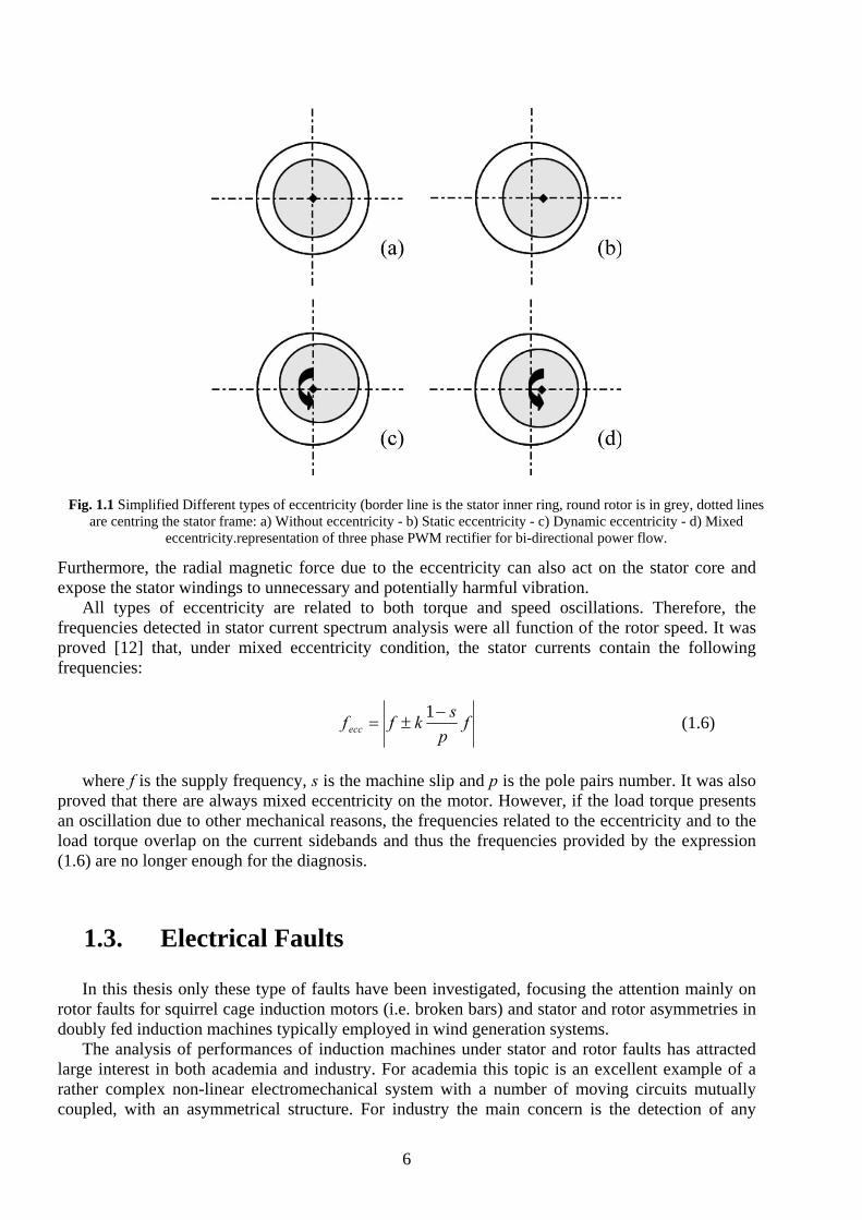
On the other hand, eccentricity faults in induction motors have been largely investigated in the last years. It is well known by mechanical engineers, that the eccentricity of a cylinder rotating around an air-gap can be classified as static, dynamic or mixed. For the static eccentricity, the center of rotation is simply displaced from the original center of a certain quantity. Then, for a dynamic eccentricity, the center of rotation is still at its origin while the cylinder is displaced. Finally, for the mixed eccentricity, both the cylinder and the center of rotation are displaced from their respective origin. Fig. 1.1 taken from [1] shows these three cases. Air gap eccentricity is one of the most common failure conditions in an induction machine. An eccentricity may be caused by many problems such as bad bearing positioning during the motor assembly, worn bearings, bent rotor shaft, operation under a critical speed creating rotor whirl [11].
The eccentricity generates a force on the rotor that attempts to pull the rotor from the stator bore [12]. It also causes excessive stressing of the machine and greatly increases the bearing wear.
6
Furthermore, the radial magnetic force due to the eccentricity can also act on the stator core and expose the stator windings to unnecessary and potentially harmful vibration.
All types of eccentricity are related to both torque and speed oscillations. Therefore, the frequencies detected in stator current spectrum analysis were all function of the rotor speed. It was proved [12] that, under mixed eccentricity condition, the stator currents contain the following frequencies:
fp
skffecc−
±=1 (1.6)
where f is the supply frequency, s is the machine slip and p is the pole pairs number. It was also
proved that there are always mixed eccentricity on the motor. However, if the load torque presents an oscillation due to other mechanical reasons, the frequencies related to the eccentricity and to the load torque overlap on the current sidebands and thus the frequencies provided by the expression (1.6) are no longer enough for the diagnosis.
1.3. Electrical Faults
In this thesis only these type of faults have been investigated, focusing the attention mainly on rotor faults for squirrel cage induction motors (i.e. broken bars) and stator and rotor asymmetries in doubly fed induction machines typically employed in wind generation systems.
The analysis of performances of induction machines under stator and rotor faults has attracted large interest in both academia and industry. For academia this topic is an excellent example of a rather complex non-linear electromechanical system with a number of moving circuits mutually coupled, with an asymmetrical structure. For industry the main concern is the detection of any
Fig. 1.1 Simplified Different types of eccentricity (border line is the stator inner ring, round rotor is in grey, dotted lines are centring the stator frame: a) Without eccentricity - b) Static eccentricity - c) Dynamic eccentricity - d) Mixed
eccentricity.representation of three phase PWM rectifier for bi-directional power flow.
7
machine failure at an early stage, in order to avoid downtime and replace damaged parts during scheduled maintenance operations, thus allowing remarkable cost reductions.
1.3.1. Stator faults
Two main classes of stator winding failures can be considered: asymmetry in the stator windings such as. an open phase failure and short-circuit of a few turns in a phase winding. The former allows the machine to operate with a reduced torque while the latter leads to a catastrophic failure in a short time. The model of the machine is a key item and is remarkably different for the two classes. In case of winding asymmetry, the winding parameters are changed in the usual machine models while in case of shorted turns, the structure of the equations changes by increasing the number of state variables.
Traditionally, an electrical or magnetic non-rotational asymmetry of induction machine or an asymmetry in the supply voltages is detected through the stator current negative sequence. The machine behaviour is not the ideal one but no drastic action must be taken in case of small asymmetries. A strong electric asymmetry, as an open phase, causes a negative sequence of the same order of magnitude of the positive one. Therefore, this last event is easily detected and the protection system is activated.
A short-circuit is recognized as one of the most difficult failures to detect. The usual protection might not act and the motor might keep on running while the heating in the shorted turns would soon cause critical insulation breakdown. If left undetected, turn faults can propagate, leading to phase-ground or phase-phase faults. Ground current flowing results in irreversible damage to the core and the machine must be removed from service. Therefore, incipient detection of turn faults is mandatory.
One of the simplest but effective method is the continuous monitoring of the negative sequence of the stator current as is usually done in case of asymmetry of the stator windings. However the main issue is still the lead time to a failure. For low voltage induction machines it is so small that an on-line diagnostic system may be useless. The worst case is a fault with a small number of shorted turns for which the lead time is around a few seconds. Counter intuitively, the lead time is just slightly increased weakening the magnetizing field [13].
A model based approach could be useful for scientific purposes and to deeply understand machine behavior but not for industrial applications. In fact, these models require a thorough knowledge of machine design parameters usually not readily available from the manufacturer. In summary, the available models are nice analytical tools helping engineers to predict machine behaviour, whereas the issue of detecting a short-circuit event with on-line measurements of a machine without interrupting its operation is an open problem.
Many proposals have been presented for the use of negative sequence current that is sensitive to different phenomena beyond stator asymmetry [14]. It is also related to the short circuit, namely, it is minimum for one shorted turn that is the worst case. An effective diagnostic procedure should distinguish between the negative sequence caused by the short circuit that must be linked to a few fundamental parameters of the machine and the negative sequence caused by unbalanced voltages, saturation and winding asymmetries.
In order to take into account the effects of unbalanced voltages [14] both current and voltage signals are acquired and a procedure is proposed with the aim to replace the usual protection with more sophisticated system, able to disconnect the machine before a complete failure. Using current and voltage signals the negative sequence impedance can be computed. The latter is quite constant unless a failure is taking place in the machine. It is suggested that a fault alarm is triggered if a deviation larger than up to 6% occurs. This threshold must be tuned in order to consider intrinsic asymmetries. To this aim a series of tests has been made in order to compute the cross-impedances between the voltage and current sequences and their variation with the machine load [15], [16]. A deep investigation on the behaviour of cross-admittance between current negative sequence and
8
voltage positive sequence is presented in [17] where a relationship is given between the amplitude of the cross admittance and the number of shorted turns.
In [18], some assumptions were made that allow computation of the negative-sequence current caused by the short circuit with a reduced number of machine parameters, provided that the number of shorted turns is very low.
For one shorted turn only the limit value for the amplitude of the negative sequence component is obtained from the following relation:
s
Nn NR
VnI
6= with 1→Nn (1.7)
where nN is the number of shorted turns, V is phase voltage, N is the number of turns per phase
and per pole, and Rs is the stator resistance. Relationship (1.7) is proposed to state a threshold current for the worst case, which is a single short-circuited turn, once the bias introduced by the intrinsic stator asymmetry and by the voltage negative sequence component has been removed.
However the threshold value is very low, thus relying on negative sequence current makes it very difficult to sense the case of a minimum number of shorted turns. For this reason diagnostic procedures based on the inverse sequence and more in general on the signature analysis of machine currents in case of stator fault are suggested to be used as a second level of diagnosis, after a proper evaluation of the insulation condition that could be performed with sophisticated techniques such as Partial Discharge (PD) activity monitoring [19].
Another interesting approach is based on the fluctuation of the space vector of the currents created by any fault unbalance [20].
Further proposals can be found in the literature looking at other current components influenced by stator winding short circuits. The use of signal injection was investigated in [21], [22] and [23] in order to diagnose stator faults in drives with different results.
In the present thesis stator faults are investigated in Doubly Fed Induction Machines. In this case also rotor currents are available and the effect of such a fault could be detected also through their signature analysis. In fact, as happen in case of rotor fault, the inverse sequence component in the stator currents provokes an electromechanical frequency propagation phenomenon which will lead to the appearance of the first fault harmonic on rotor currents at frequency (2-s)f where f is the supply frequency and s is the slip. The resulting chain of frequency due to such an electromechanical interaction will be presented in the next paragraph for rotor faults and will be subsequently detailed in chapter 4 in case of stator faults. It’s worth noting that all the above considerations are done neglecting the impact of the control system usually employed in variable speed drives.
1.3.2. Rotor faults
Two different types of squirrel-cage rotors exist in induction motors, namely, cast and fabricated. Fabricated cages are used for very high ratings and special application machines where possible failure events occur on bars and end-ring segments. Cast rotors are almost impossible to repair after bar breakage or cracks although they are more durable and rugged than fabricated cages. Typically, they are used in laboratory tests to validate diagnostic procedures for practical reasons. Broken bar and cracked end ring faults share only 5–10 % of induction machine faults but the detection of these events is a key issue.
While in case of stator faults machine operation after the fault is limited to a few seconds, in case of rotor faults the machine operation after the fault is not restricted. On the other hand, the current in the rotor bar adjacent to the faulty one increases up to 50 % of rated current leading to potential further breakage and stator faults as well. In summary, an accurate detection of rotor faults
9
may lead to a complete diagnostic process whereas the fault detection of stator winding faults can lead only to an intelligent protection system.
Motor current signature analysis (MCSA) has being extensively used to detect broken rotor bar and end ring faults in induction machines. It is well known from the rotating field theory that any rotor asymmetry generates a component at (1-2s)f in the stator current spectrum with the assumption of constant speed or infinite inertia where f is the frequency of supply voltages, and s is the machine slip. Removing these assumptions a component at (1+2s)f appears in the current spectrum as confirmed by experiments. An effective diagnostic procedure must take into account for both components [24].
In [25], an insightful analysis of the link between the sideband component amplitude and the rotor asymmetry is presented. The cause to effect chain was theoretically proved as follows.
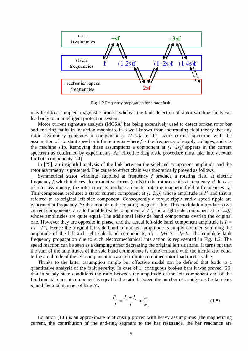
Symmetrical stator windings supplied at frequency f produce a rotating field at electric frequency f, which induces electro-motive forces (emfs) in the rotor circuits at frequency sf. In case of rotor asymmetry, the rotor currents produce a counter-rotating magnetic field at frequencies -sf. This component produces a stator current component at (1-2s)f, whose amplitude is I’l and that is referred to as original left side component. Consequently a torque ripple and a speed ripple are generated at frequency 2sf that modulate the rotating magnetic flux. This modulation produces two current components: an additional left-side component at I’’l and a right side component at (1+2s)f, whose amplitudes are quite equal. The additional left-side band components overlap the original one. However they are opposite in phase, and the actual left-side band component amplitude is Il = I’l – I’’l. Hence the original left-side band component amplitude is simply obtained summing the amplitude of the left and right side band components, I’l = Il+I’’l = Il+Ir. The complete fault frequency propagation due to such electromechanical interaction is represented in Fig. 1.2. The speed reaction can be seen as a damping effect decreasing the original left sideband. It turns out that the sum of the amplitudes of the side band components is quite constant with the inertia and equal to the amplitude of the left component in case of infinite combined rotor-load inertia value.
Thanks to the latter assumption simple but effective model can be defined that leads to a quantitative analysis of the fault severity. In case of nr contiguous broken bars it was proved [26] that in steady state conditions the ratio between the amplitude of the left component and of the fundamental current component is equal to the ratio between the number of contiguous broken bars nr and the total number of bars Nr.
r
rrll
Nn
III
II
≈+
='
(1.8)
Equation (1.8) is an approximate relationship proven with heavy assumptions (the magnetizing
current, the contribution of the end-ring segment to the bar resistance, the bar reactance are
Fig. 1.2 Frequency propagation for a rotor fault.

10
neglected). However, it is nicely in agreement with experimental results obtained with large machines [27].
Two phenomena that could affect the extension of the fault by means of (1.8) are the effect of saturation and interbar currents. Saturation produces a third harmonic in the rotor current. Consequently a component at (1+2s)f appears in the stator current leading to a frequency propagation phenomenon that could affect the proper detection and quantification of the fault [28].
On the other hand, interbar currents tends to mask the asymmetry produced by a bar breakage leading to an under estimate of the rotor fault extension.
Different approaches can be found in literature using multiple electric signals. A very famous one which was also designed to diagnose rotor faults in vector-controlled induction motor drives is the so called Vienna monitoring method (VMM) [29]. This technique relies on voltage, current signals and measured rotor position to check deviations in terms of instantaneous torque obtained by two different machine models. This procedure was proposed as a quantitative diagnostic index independent of inertia and load.
Finally Other techniques can be found relying on the rotor resistance variation estimation[30], instantaneous power spectral analysis [31] and high frequency signal injection [32],[21] for the detection of rotor faults in squirrel cage induction motors.
11
Chapter 2
Induction Motor Models
2.1. Introduction
The models developed for the squirrel cage induction machine and the doubly fed induction generator take into account only the fundamental spatial component of the air-gap magnetic field. Such an approximation allows anyway to study the phenomenon of the fault frequency propagation discussed in the previous chapter in case of stator and rotor faults without losing generality. This choice was done since the presence of terms with an infinite number of space harmonics in a large system of differential equations would lead to heavy computational demand for a model that has to be coupled with a control system simulation scheme implemented in a suitable environment such as MATLAB Simulink.
Alternative approaches that could effectively take into account the effect of all space harmonics increasing the model in complexity are:
• The winding function approach [33] where the linkage and the leakage inductances can
be computed for arbitrary winding layout or for unbalanced operating conditions. Moreover slotting, skewing and saturation can be modeled and simulated by means of a suitable air-gap function.
• Dynamic mesh reluctance approach [13] where the machine is geometrically divided into flux tubes whose reluctances are non-linear functions of the magnetic potential.
• Finite Element approach [34],[35] for which the geometry of the machine (air-gap, core) is discretized in element with limit conditions. Then, the field computation can lead to torque, flux and even current evaluation.
2.2. Simulation Environment (Simulink® S-function)
Matlab Simulink was chosen for the implementation of the machine models and the control algorithms for the variable speed drives under investigation. The choice of this environment was made due to its simplicity in developing control schemes thanks to the embedded sets of blocks that can be easily connected through a simple graphical user interface. Moreover Simulink® offers
12
libraries such as the SimPowerSystem library, which furnish a series of built-in blocks for the simulation of electrical systems such as power electronics converters and machines. Unfortunately those models are not enough accurate for the study of the faults in electrical machines.
An interesting block of Simulink, i.e. the S-Function block, was used to overcome these limitations. Such a block was born specifically to implement continuous and discrete systems in the input-state-output form. Hence, Matlab user can employ S-Functions to implement systems which are not present in Simulink library writing them in M-code.
More in general S-functions provide a powerful mechanism for extending the capabilities of the Simulink® environment. An S-function is a computer language description of a Simulink block written in MATLAB®, C, C++, Ada, or Fortran. C, C++, Ada, and Fortran S-functions are compiled as MEX-files (MATLAB executable files) by using the mex utility. As with other MEX-files, S-functions are dynamically linked subroutines that the MATLAB® interpreter can automatically load and execute.
S-functions follow a general form and can accommodate continuous, discrete, and hybrid systems. By following a set of simple rules, it is possible implement an algorithm in an S-function and use the S-Function block in a Simulink model.
In our case the S-function block will be used to implement the set of differential equations derived from the developed machine models in order to exploit the MATLAB® variable step ODE (Ordinary Differential Equations) solvers. As said this set of differential equations has to be expressed in the input-state-output form.
2.3. Squirrel Cage Induction Machine Model
2.3.1. Introduction
In order to test the effectiveness of the rotor faults diagnostic procedures, that will be later discussed, a transient model of the faulty squirrel cage induction machine is required [36]. To develop a general model, the actual geometry of the rotor must be considered. The N bars and the 2N end ring segments constitute a network with N+1 loops with N independent mesh currents and a circulating current in one of the end rings. The values of the electrical parameters are identical for all the loops under healthy operating conditions but obviously differ if a break occurs. Therefore the machine can be modelled as a system of multiple coupled circuits. When this approach is used, it is necessary to compute the mutual inductance coefficients, which are dependent on the rotor position. This model is referred to a reference frame rotating with the rotor, therefore rotational dynamic emf terms are only present on stator windings voltage equations. The assumed stator and rotor m.m.f. distributions allow an easy determination of the stator-stator, stator-rotor and rotor-rotor mutual inductances. In the next section the main assumptions related to the model are described, and the computation of the mutual inductance coefficient is discussed.
2.3.2. Machine Model
The following assumptions are used for the derivation of the mathematical model of the single-cage induction machine which is suitable for the analysis of various cage faults:
• Infinite iron permeability • Smooth air gap • quadrature-phase symmetrical stator windings with sinusoidal distribution of the air gap flux
density

13
• Rotor windings originally form a symmetrical cage, the bars are insulated from the iron core. The assumption of the two phase stator is not strictly necessary. Anyway the model does not
loose in generality if rotor faults are considered. The assumption of insulated bars is necessary to neglect the interbar currents which may flow in the iron core when a bar breaks. The self and mutual inductance coefficients of the two stator circuits and the N+1 rotor loops shown in Fig. 2.1, are computed by using theory of space vectors and the assumptions discussed above. For the analysis a reference frame fixed to the rotor is chosen.
The assumption of sinusoidal flux distribution for the two stator circuit leads to the following well known expression for the stator self inductance by taking into account the magnetic field lines that cross the air gap:
δ
μπ 2
21
23P
LDNKM w
s 0= (2.1)
where µ0 is the vacuum permeability, N1 is the number of turns in series per phase, L is the machine length, D is the air-gap diameter, P is the number of pole pairs, δ is the air-gap and Kw is the winding factor given by the product of the distribution and pitch factors:
)2cos()2sin()2sin( ψ
γγ
qqKw = (2.2)
In (2.2) γ is the electrical pitch angle between two adjacent stator slots, ψ is the electrical coil-
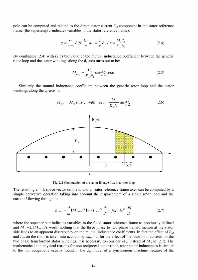
span angle and q is the number of slots per pole per phase. In the adopted reference frame the derivative of the rotor angular position θ(t), ω, introduces motional terms ωMs in the stator voltage equations. The sinusoidal flux density distribution of the stator windings give rise to a sinusoidal rotor flux linkage. The value of Ms can be used to calculate the stator-rotor mutual inductance coefficient as explained hereafter. With reference to Fig. 2.2, where the ds-axis of the two phase stator windings is taken as a reference, the stator flux linkage in a single generic rotor loop is:
θατπ
υπτυϕ
αθ
αθcos2sin2)(
2/
2/∫+
−== LBdLB Mrl (2.3)
where τ is the pole pitch, BM is the maximum value of the magnetic flux density sinusoidal distribution and α=2πP/N is the electric angle of a single rotor loop. In the same way the flux per
ds
qs
ei
rii
Fig. 2.1 Stator Windings and rotor loops of the model
14
pole can be computed and related to the direct stator current issd component in the stator reference
frame (the superscript s indicates variables in the stator reference frame):
1
2/
2/
2)(NKiMLBdLB
w
ssds
M === ∫−π
πτ
πυ
πτυϕ (2.4)
By combining (2.4) with (2.3) the value of the mutual inductance coefficient between the generic rotor loop and the stator windings along the ds-axis turns out to be:
θα cos2sin1NK
MMw
srsds
= (2.5)
Similarly the mutual inductance coefficient between the generic rotor loop and the stator
windings along the qs-axis is:
θsinrsrsq MMs= , with 2sin
1
αNK
MMw
srs = (2.6)
The resulting e.m.f. space vector on the ds and qs stator reference frame axes can be computed by a simple derivative operation taking into account the displacement of a single rotor loop and the current i flowing through it:
( )dtdiejM
dtdieMieM
dtde j
srj
srj
srsdqs θθθθ ''' +== (2.7)
where the superscript s indicates variables in the fixed stator reference frame as previously defined and M’
sr=2/3Mrs. It’s worth nothing that the three phase to two phase transformation at the stator side leads to an apparent discrepancy on the mutual inductance coefficients. In fact the effect of is
sd and is
sq on the rotor is taken into account by Mrs, but for the effect of the rotor loop currents on the two phase transformed stator windings, it is necessary to consider M’
sr instead of Mrs in (2.7). The mathematical and physical reasons for non reciprocal stator-rotor, rotor-stator inductances is similar to the non reciprocity usually found in the dq model of a synchronous machine because of the
B(θ)
τ
θ
BM
α/2
Fig. 2.2 Computation of the stator linkage flux in a rotor loop
15
asymmetrical form of the space vector equations [36]. Equation (2.7) can be rewritten in terms of d-q components as follows:
θωθ
θωθ
cossin
sincos
''
''
srsrq
srsrd
MdtdiMe
MdtdiMe
s
s
+=
−= (2.8)
where the derivative of θ has been substituted by the rotor electrical speed ω. Due to the reference frame chosen for the mathematical model (rotor reference frame) the e.m.f. appearing in the rotor voltage equations contains only the transformer terms. Moreover, when stator and rotor equations are related to the same rotor reference frame, the dependence on the rotor electrical angle disappears.
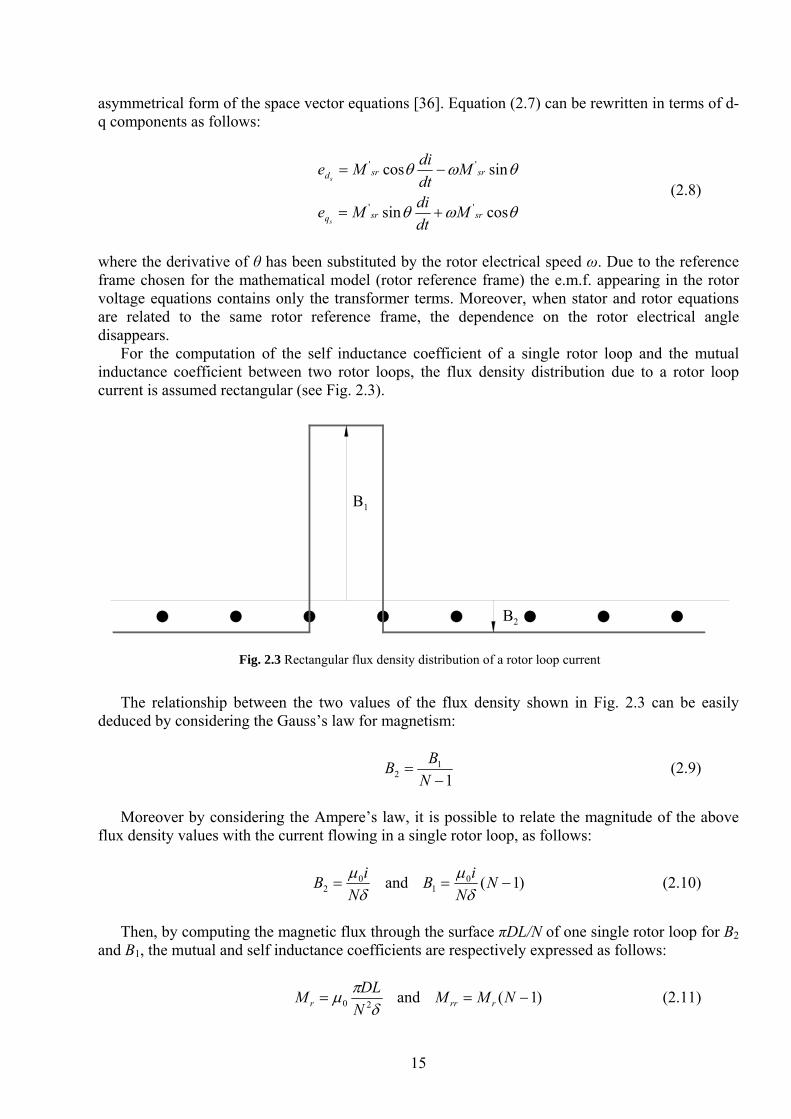
For the computation of the self inductance coefficient of a single rotor loop and the mutual inductance coefficient between two rotor loops, the flux density distribution due to a rotor loop current is assumed rectangular (see Fig. 2.3).
The relationship between the two values of the flux density shown in Fig. 2.3 can be easily
deduced by considering the Gauss’s law for magnetism:
1
12 −=
NBB (2.9)
Moreover by considering the Ampere’s law, it is possible to relate the magnitude of the above
flux density values with the current flowing in a single rotor loop, as follows:
δ
μN
iB 02 = and )1(0
1 −= NN
iBδ
μ (2.10)
Then, by computing the magnetic flux through the surface πDL/N of one single rotor loop for B2
and B1, the mutual and self inductance coefficients are respectively expressed as follows:
δ
πμ 20 NDLM r = and )1( −= NMM rrr (2.11)
B1
B2
Fig. 2.3 Rectangular flux density distribution of a rotor loop current
16
The remaining parameters, i.e. stator winding resistance Rs, rotor bar resistance Rb, end ring resistance, stator leakage inductance lds, rotor bar leakage inductance ldb and end ring leakage inductance lde can be computed by using well known formulae. For this purpose the details of machine design must be known. However, when the motor design parameters are unknown a possible procedure is to utilize the usual rotor parameters referred to stator windings (these are the equivalent resistance Rr and the equivalent leakage inductance ldr). The relationships for the computation of Rr and ldr starting from Rb, Re, ldb and lde are well established. The inverse procedure needs assumptions about the distribution of the rotor parameters between the bar and the end rings. By assuming Rb=Re and ldb=lde:
( ) ⎟⎟⎠
⎞⎜⎜⎝
⎛+
==
2
21
)2sin(221)(12αNN
KNRRR
w
reb (2.12)
( ) ⎟⎟⎠
⎞⎜⎜⎝
⎛+
==
2
21
)2sin(221)(12αNN
KNlll
w
drdedb (2.13)
It has been shown in [26] that the distribution of the parameters has a limited influence on the
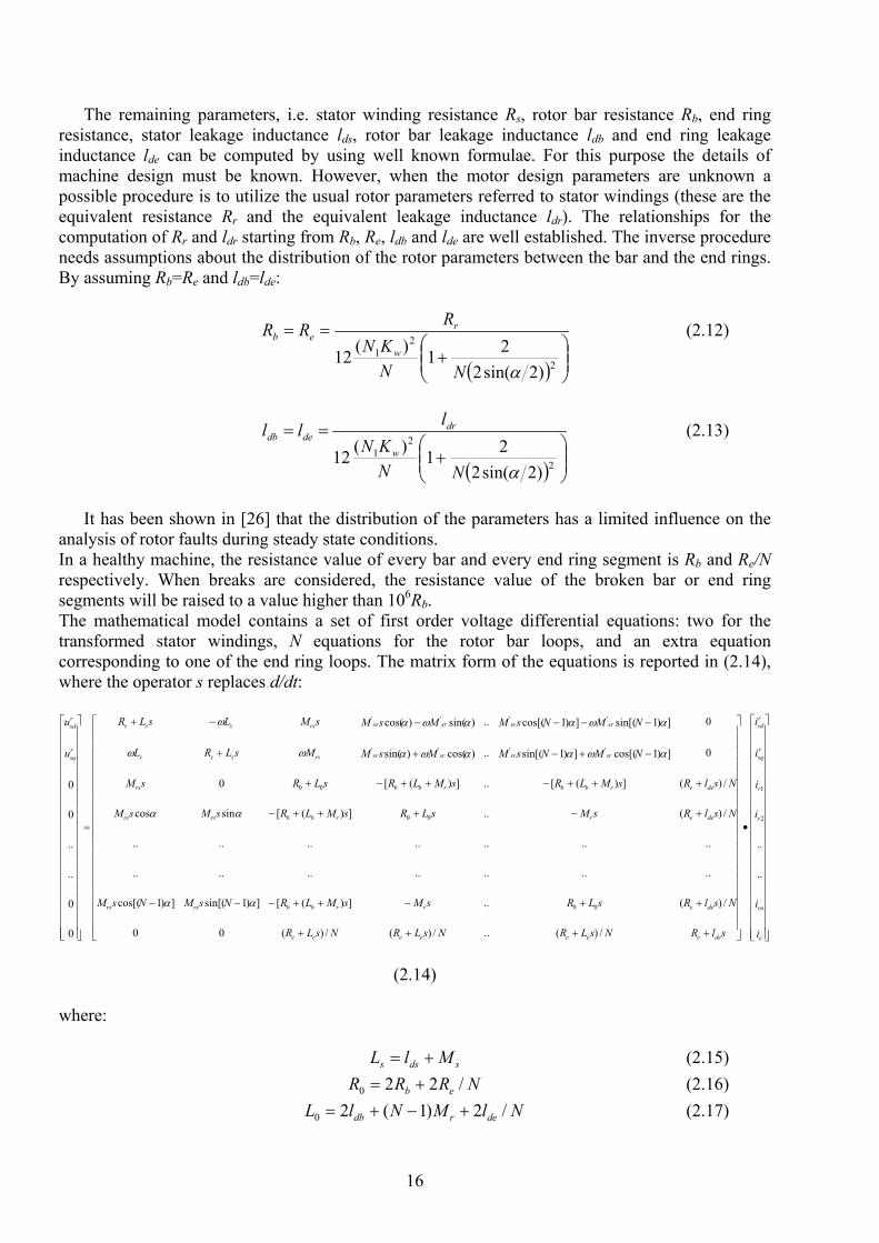
analysis of rotor faults during steady state conditions. In a healthy machine, the resistance value of every bar and every end ring segment is Rb and Re/N respectively. When breaks are considered, the resistance value of the broken bar or end ring segments will be raised to a value higher than 106Rb. The mathematical model contains a set of first order voltage differential equations: two for the transformed stator windings, N equations for the rotor bar loops, and an extra equation corresponding to one of the end ring loops. The matrix form of the equations is reported in (2.14), where the operator s replaces d/dt:
⎥⎥⎥⎥⎥⎥⎥⎥⎥⎥⎥⎥⎥⎥⎥⎥⎥⎥⎥⎥
⎦
⎤
⎢⎢⎢⎢⎢⎢⎢⎢⎢⎢⎢⎢⎢⎢⎢⎢⎢⎢⎢⎢
⎣
⎡
•
⎥⎥⎥⎥⎥⎥⎥⎥⎥⎥⎥⎥⎥⎥⎥⎥⎥⎥⎥
⎦
⎤
⎢⎢⎢⎢⎢⎢⎢⎢⎢⎢⎢⎢⎢⎢⎢⎢⎢⎢⎢
⎣
⎡
++++
++−++−−−
+−+++−
+++−++−+
−+−++
−−−−−+
=
⎥⎥⎥⎥⎥⎥⎥⎥⎥⎥⎥⎥⎥⎥⎥⎥⎥⎥⎥⎥
⎦
⎤
⎢⎢⎢⎢⎢⎢⎢⎢⎢⎢⎢⎢⎢⎢⎢⎢⎢⎢⎢⎢
⎣
⎡
e
rn
r
r
rsq
rsd
deeeeeeee
deerrbbrsrs
deerrbbrsrs
deerbbrbbrs
srsrsrsrrssss
srsrsrsrrssss
rsq
rsd
i
i
i
i
i
i
slRNsLRNsLRNsLR
NslRsLRsMsMLRNsMNsM
NslRsMsLRsMLRsMsM
NslRsMLRsMLRsLRsM
NMNsMMsMMsLRL
NMNsMMsMsMLsLR
u
u
..
..
/)(../)(/)(00
/)(..])([])1sin[(])1cos[(
..............
..............
/)(..])([sincos
/)(])([..])([0
0])1cos[(])1sin[(..)cos()sin(
0])1sin[(])1cos[(..)sin()cos(
0
0
..
..
0
0
2
1
00
00
00
''''
''''
αα
αα
αωααωαωω
αωααωαω
(2.14)
where:
sdss MlL += (2.15) NRRR eb /220 += (2.16) NlMNlL derdb /2)1(20 +−+= (2.17)
17
are the total stator inductance, the total rotor loop resistance and the total rotor loop inductance respectively. The rotor loop currents are represented by ir1, ir2, ir3,...irN, whereas the end ring current by ie.
The input voltages of the system are defined by:
⎥⎥⎦
⎤
⎢⎢⎣
⎡⎥⎦
⎤⎢⎣
⎡−
=⎥⎥⎦
⎤
⎢⎢⎣
⎡ssq
ssd
rsq
rsd
u
u
u
uθθθθ
cossinsincos
(2.18)
where the superscript r refers to variables in the rotor reference frame. In case of open loop operations, i.e. machine supplied by the grid, the input voltages are as follow:
tVu s
ssd ωcos2= and tVu s
ssq ωsin2= with ss fπω 2= (2.19)
Equations (2.14) can be used to simulate the transient electrical state if ω is considered as an
input. However, for the simulation of the transient electromechanical state, two further equations must be considered:
2
⎟⎠⎞
⎜⎝⎛−−=
PKTT
dtd
PJ
alemωω (2.20)
ωθ=
dtd (2.21)
where J is the moment of inertia Tl is the load torque and the electromagnetic torque Tem has the following expression:
( )
( ) rsdrNsrrsrrsr
rsqrNsrrsrrsrrsrem
iNiMiMiMP
iNiMiMiMiMPT
ααα
ααα
)1sin(...2sinsin23
)1cos(...2coscos23
'3
'2
'
'3
'2
'1
'
−+++−
+−++++=(2.22)
In (2.22) the torque is independent of the chosen reference frame and in (2.20) a viscous friction
torque has been added to the load torque Tl. The quadrature-axis stator currents in the stationary reference frame can be obtained from ir
sd and irsq by using the well known transformation:
⎥⎥⎦
⎤
⎢⎢⎣
⎡⎥⎦
⎤⎢⎣
⎡ −=
⎥⎥⎦
⎤
⎢⎢⎣
⎡rsq
rsd
ssq
ssd
i
i
i
iθθθθ
cossinsincos
(2.23)
It should be noted that it is possible to implement also a non transformed model of the cage
machine (3+N+1 voltage equations, which contain three stator voltage equations, expressed in the stationary reference frame, and N+1 rotor equations expressed in the rotor reference frame). However, these equations would contain the rotor angle θ, e.g. the fourth element in the first column of the impedance matrix in (2.14) would be M’srscosθ, etc. In this case the mutual inductance coefficients would be reciprocal. The electromagnetic torque could be computed similarly to that shown above by using two axis stator flux components and currents, or by using a technique where the torque matrix T is utilized, where T=dL/dθ is the derivative of the inductance
18
matrix (a similar approach will be used later for the other machine model developed in our study). Thus the fourth element in the first column of T would contain –sinθ.
As said in paragraph 2.2 the machine model equations (2.14), (2.20) and (2.21) have to be expressed in explicit form (i.e. in the input state output form) in order to be implemented. Since the impedance matrix contains the electrical speed of the rotor, which is a state variable, the inverse of such a matrix should be calculated at each simulation step. This time consuming computational operation can be avoided. In fact it is possible to split the impedance matrix into two matrixes: the first one containing all the speed dependent terms [R(ω)] and a second one [Ds] including all the terms containing the Laplace operator s. In this way (2.14) can be formulated as follows using concise matrix notation:
]][[])][([][ IDIRU s
&+= ω (2.24)
where [U] is the voltage vector and [I] is the current vector containing the two stator currents, the N rotor loop currents and one end-ring current. The input-state-output form can be obtained by inversing the [Ds] matrix just once at the beginning of the simulation, since no state variables are present in it. Thus the explicit form of (2.24) results in:
]][[])][(][[][ 11 UDIRDI ss
−− +−= ω& (2.25) Finally by considering also equations (2.20) and (2.21), which are already in explicit form, the
entire model presents: • three inputs, i.e. two stator voltages and the load torque • N+5 state variables, i.e. two stator currents, N rotor loop currents, one end ring current and
two mechanical variables, the electrical rotor speed and angle • N+5 outputs, i.e. N bar currents computed as the difference between currents of two adjacent
rotor loops, the electromagnetic torque, the two stator currents in the stator reference frame, the electrical rotor speed and angle.
Once the model has been implemented a comparison with an already validated classical dq
model in the rotor reference frame, whose equations are presented in (2.26), was performed.
⎥⎥⎥⎥⎥
⎦
⎤
⎢⎢⎢⎢⎢
⎣
⎡
•
⎥⎥⎥⎥⎥
⎦
⎤
⎢⎢⎢⎢⎢
⎣
⎡
++
+−−+
=
⎥⎥⎥⎥⎥
⎦
⎤
⎢⎢⎢⎢⎢
⎣
⎡
rrq
rrd
rsq
rsd
rrrs
rrrs
rsrssss
rsrssssrsq
rsd
iiii
sLRsMsLRsM
sMMsLRLMsMLsLR
uu
0000
00
ωωωω
(2.26)
The aim of this comparison was to investigate the validity of the assumption regarding space
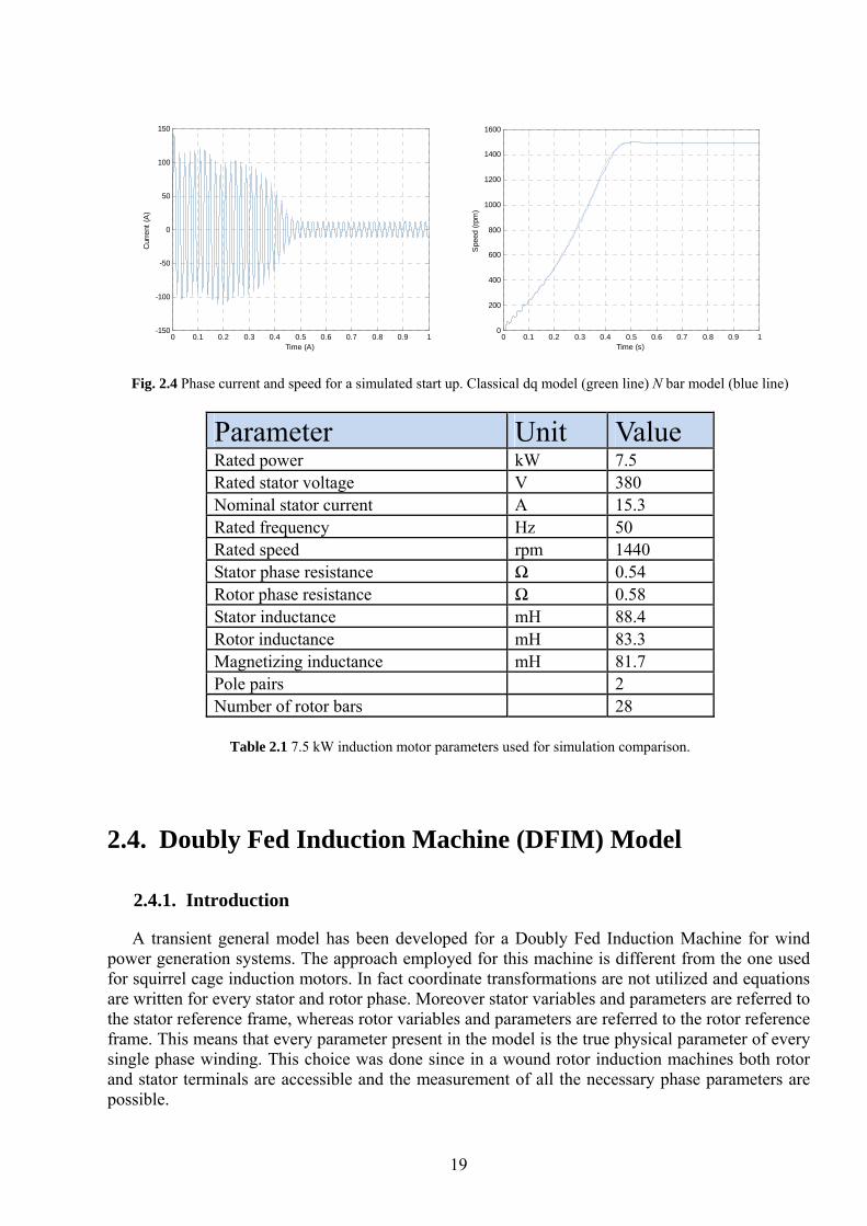
harmonics. As known, model (2.26) is related to two stator windings and to two rotor windings with sinusoidal air gap flux density distribution. Considering a model with N rotor loops with rectangular flux density distribution would lead to some discrepancies. Anyway the assumption becomes more and more acceptable by increasing the rotor bar numbers as proved in [36]. Fig. 2.4 shows the comparison of a simulated motor start-up for the two models. It’s evident that the discrepancy between them is negligible. Motor data are reported in Table 2.1.
19
2.4. Doubly Fed Induction Machine (DFIM) Model
2.4.1. Introduction
A transient general model has been developed for a Doubly Fed Induction Machine for wind power generation systems. The approach employed for this machine is different from the one used for squirrel cage induction motors. In fact coordinate transformations are not utilized and equations are written for every stator and rotor phase. Moreover stator variables and parameters are referred to the stator reference frame, whereas rotor variables and parameters are referred to the rotor reference frame. This means that every parameter present in the model is the true physical parameter of every single phase winding. This choice was done since in a wound rotor induction machines both rotor and stator terminals are accessible and the measurement of all the necessary phase parameters are possible.
0 0.1 0.2 0.3 0.4 0.5 0.6 0.7 0.8 0.9 1-150
-100
-50
0
50
100
150
Time (A)
Cur
rent
(A)
0 0.1 0.2 0.3 0.4 0.5 0.6 0.7 0.8 0.9 10
200
400
600
800
1000
1200
1400
1600
Time (s)
Spe
ed (r
pm)
Fig. 2.4 Phase current and speed for a simulated start up. Classical dq model (green line) N bar model (blue line)
Parameter Unit Value Rated power kW 7.5 Rated stator voltage V 380 Nominal stator current A 15.3 Rated frequency Hz 50 Rated speed rpm 1440 Stator phase resistance Ω 0.54 Rotor phase resistance Ω 0.58 Stator inductance mH 88.4 Rotor inductance mH 83.3 Magnetizing inductance mH 81.7 Pole pairs 2 Number of rotor bars 28
Table 2.1 7.5 kW induction motor parameters used for simulation comparison.
20
Representing motor variables in two different reference frames will make the impedance matrix dependent on the rotor electrical angle. Anyway on the hypothesis of null homopolar current component the number of equations is reduced to six, i.e. four voltage equations and two mechanical equations.
2.4.1. DFIM model
For the derivation of the mathematical model the following assumptions are considered: • Infinite iron permeability • Smooth air gap • three-phase symmetrical stator and rotor windings with sinusoidal distribution of the air gap
flux density Starting from the equation in the time domain for every single stator and rotor winding we can
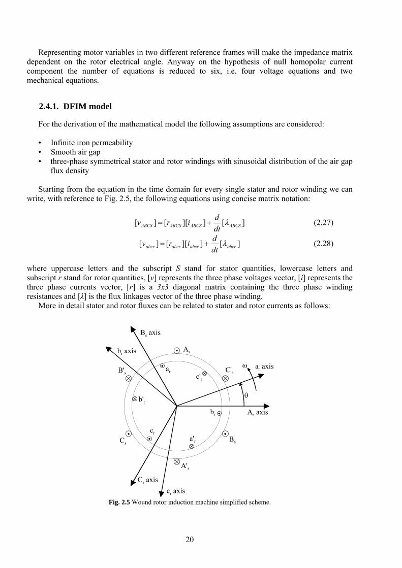
write, with reference to Fig. 2.5, the following equations using concise matrix notation:
][]][[][ ABCSABCSABCSABCS dtdirv λ+= (2.27)
][]][[][ abcrabcrabcrabcr dtdirv λ+= (2.28)
where uppercase letters and the subscript S stand for stator quantities, lowercase letters and subscript r stand for rotor quantities, [v] represents the three phase voltages vector, [i] represents the three phase currents vector, [r] is a 3x3 diagonal matrix containing the three phase winding resistances and [λ] is the flux linkages vector of the three phase winding.
More in detail stator and rotor fluxes can be related to stator and rotor currents as follows:
As axis
Bs axis
Cs axis
ar axis
br axis
cr axis
As
A's
Bs
B's
Cs
C'sar
a'r
b'rbr
cr
c'r
θ
ω
Fig. 2.5 Wound rotor induction machine simplified scheme.
21
⎥⎦
⎤⎢⎣
⎡⎥⎦
⎤⎢⎣
⎡=⎥
⎦
⎤⎢⎣
⎡
abcr
ABCS
rT
Sr
SrS
abcr
ABCS
ii
LLLL
][)]([)]([][
θθ
λλ
(2.29)
where [Ls], [Lr] and [Lsr(θ)] represents the following matrixes of self and mutual inductance coefficients:
⎥⎥⎥
⎦
⎤
⎢⎢⎢
⎣
⎡=
CSBCSACS
BCSBSABS
ACSABSAS
S
LMMMLMMML
L ][ (2.30)
⎥⎥⎥
⎦
⎤
⎢⎢⎢
⎣
⎡=
crbcracr
bcrbrabr
bcrabrar
r
LMMMLMMML
L ][ (2.31)
⎥⎥⎥⎥⎥⎥⎥
⎦
⎤
⎢⎢⎢⎢⎢⎢⎢
⎣
⎡
⎟⎠⎞
⎜⎝⎛ −⎟
⎠⎞
⎜⎝⎛ +
⎟⎠⎞
⎜⎝⎛ +⎟
⎠⎞
⎜⎝⎛ −
⎟⎠⎞
⎜⎝⎛ −⎟
⎠⎞
⎜⎝⎛ +
=
θπθπθ
πθθπθ
πθπθθ
θ
cos3
2cos3
2cos
32coscos
32cos
32cos
32coscos
)]([
SrCcSrCbSrCa
SrBcSrBbSrBa
SrAcSrAbSrAa
Sr
LLL
LLL
LLL
L (2.32)
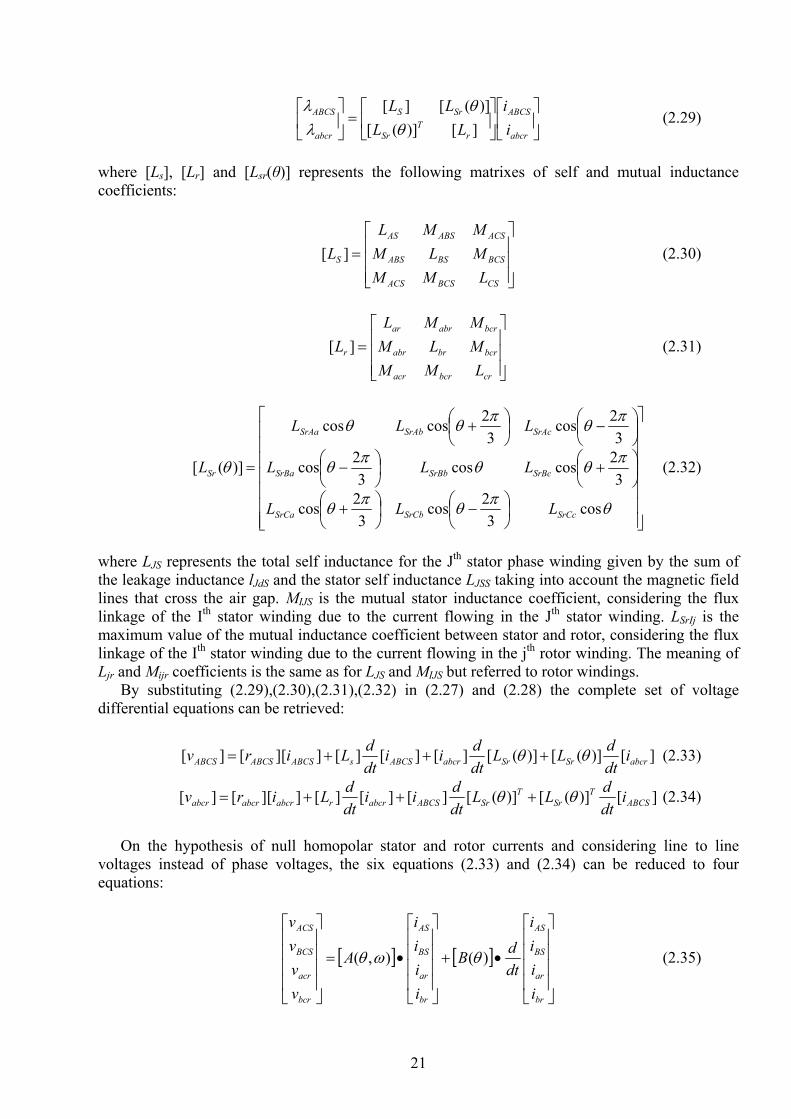
where LJS represents the total self inductance for the Jth stator phase winding given by the sum of the leakage inductance lJdS and the stator self inductance LJSS taking into account the magnetic field lines that cross the air gap. MIJS is the mutual stator inductance coefficient, considering the flux linkage of the Ith stator winding due to the current flowing in the Jth stator winding. LSrIj is the maximum value of the mutual inductance coefficient between stator and rotor, considering the flux linkage of the Ith stator winding due to the current flowing in the jth rotor winding. The meaning of Ljr and Mijr coefficients is the same as for LJS and MIJS but referred to rotor windings.
By substituting (2.29),(2.30),(2.31),(2.32) in (2.27) and (2.28) the complete set of voltage differential equations can be retrieved:
][)]([)]([][][][]][[][ abcrSrSrabcrABCSsABCSABCSABCS idtdLL
dtdii
dtdLirv θθ +++= (2.33)
][)]([)]([][][][]][[][ ABCST
SrT
SrABCSabcrrabcrabcrabcr idtdLL
dtdii
dtdLirv θθ +++= (2.34)
On the hypothesis of null homopolar stator and rotor currents and considering line to line
voltages instead of phase voltages, the six equations (2.33) and (2.34) can be reduced to four equations:
[ ] [ ]⎥⎥⎥⎥
⎦
⎤
⎢⎢⎢⎢
⎣
⎡
•+
⎥⎥⎥⎥
⎦
⎤
⎢⎢⎢⎢
⎣
⎡
•=
⎥⎥⎥⎥
⎦
⎤
⎢⎢⎢⎢
⎣
⎡
br
ar
BS
AS
br
ar
BS
AS
bcr
acr
BCS
ACS
iiii
dtdB
iiii
A
vvvv
)(),( θωθ (2.35)
22
where matrix [A(θ,ω)] contains all the e.m.f. motional terms, whereas all the transformer terms are confined in [B(θ)]. For the sake of brevity these two matrixes are not presented here since they add very little to the discussion. Anyway they can be easily derived from equations (2.33) and (2.34).
For the simulation of the transient electromechanical state also the two mechanical equations (2.20) and (2.21) have to be added to the system. The electromagnetic torque can be computed as follows:
][)]([][ abcrSrT
ABCSem id
LdiTθθ
= (2.36)
Once the set of differential equations (2.35) has been expressed in explicit form (i.e. in the
input-state-output form), and the two mechanical equations (2.20) and (2.21) are taken into account, the entire model presents:
• five inputs, i.e. two stator line to line voltages, two rotor line to line voltages and the load
torque • six state variables, i.e. two stator currents, two rotor currents, and two mechanical variables,
the electrical rotor speed and angle • six outputs, i.e. the two stator currents in the stator reference frame, two rotor currents in the
rotor reference frame, the electrical rotor speed and the electromagnetic torque. It’s worth noting that, since the voltage equations are written in two different reference frames,
the impedance matrixes in (2.35) are dependent on the rotor electrical position angle. Thus to obtain the explicit form of the voltage differential equations set, matrix [B(θ)] has to be inversed at each simulation step.
23
Chapter 3
Variable Speed Drives
3.1. Introduction
On-line diagnosis and early detection of faults in induction machine drives have drawn the attention of researchers, since they allow to reduce maintenance costs and down-times. In some applications, where continuous operation is a key factor, such as railway applications and wind generation, the need for a preventive fault diagnosis is an extremely important point. Anyway the majority of the diagnostic techniques found in literature are addressed to fault detection in mains-supplied machines. These techniques present two main drawbacks: they do not take into account time varying conditions and most of all they neglect the influence of the control system on the machine variables. As a consequence such diagnostic procedures already developed for open loop operating conditions, may reveal themselves less effective or unable to perform a proper fault detection and quantification if the entire drive is considered.
With reference to closed-loop induction machine drives with a digital control system, as the control itself affects the behaviour of motor variables, new diagnostic procedures must be adopted to perform the machine monitoring. In fact the diagnostic technique has to be tailored for a specific induction motor variable speed drive application. For this reason the effect of a fault must be studied by taking into account the entire drive system.
In this chapter the control systems for two specific applications involving induction motors are presented. Field oriented control (FOC) theory is used to develop both control algorithms. Firstly a Doubly Fed Induction Machine (DFIM) based drive for Variable Speed Constant Frequency (VSCF) generation systems, usually employed in wind turbines, is discussed. Secondly the control scheme for a squirrel cage induction motor employed in railway traction systems is presented. In both cases the control algorithms have been verified by computer simulations and by laboratory tests to investigate the impact of the control system on faulty machine variables and to validate the diagnostic procedures that will be discussed in the next chapter.
24
3.2. Wind Generation Systems
3.2.1. Power scheme
Nowadays wind energy is one of the most promising among renewable energy sources and has expanded rapidly throughout the world. With the advancement of aerodynamic designs, wind turbines that can capture several megawatts of power are available. When such wind energy conversion systems (WECSs) are integrated to the grid, they produce a substantial amount of power, which can supplement the base power generated by thermal, nuclear, or hydro power plants.
A WECS can vary in size from several megawatts to a few hundred kilowatts or even less if we consider microeolic power generation. The size of the WECS largely determines the choice of the generator and converter system. Among the electrical rotating machines, induction machine have a special importance due to their simplicity and their robustness. In a comparison with alternative schemes the Doubly Fed Induction Machine (DFIM) for Variable Speed Constant Frequency generation systems are nowadays an established technology [37]. Anyway other solutions based on direct-driven permanent magnet synchronous machines are proposed on the market.
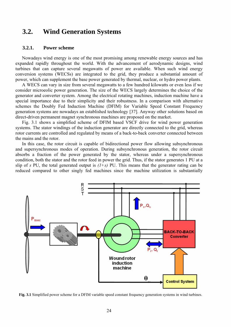
Fig. 3.1 shows a simplified scheme of DFIM based VSCF drive for wind power generation systems. The stator windings of the induction generator are directly connected to the grid, whereas rotor currents are controlled and regulated by means of a back-to-back converter connected between the mains and the rotor.
In this case, the rotor circuit is capable of bidirectional power flow allowing subsynchronous and supersynchronous modes of operation. During subsynchronous generation, the rotor circuit absorbs a fraction of the power generated by the stator, whereas under a supersynchronous condition, both the stator and the rotor feed in power the grid. Thus, if the stator generates 1 PU at a slip of s PU, the total generated output is (1+s) PU. This means that the generator rating can be reduced compared to other singly fed machines since the machine utilization is substantially
Fig. 3.1 Simplified power scheme for a DFIM variable speed constant frequency generation systems in wind turbines.
25
improved. In fact in this case the rated torque is maintained even at supersynchronous speeds whereas, in a system using cage rotor machine, field weakening has to be employed beyond synchronous speed, leading to torque reduction.
Moreover the use of a slip-ring induction generator is economically competitive, when compared to a cage rotor induction machine. The higher cost of the machine due to the slip rings is compensated by a reduction in the sizing of the power converters which has to be designed for a fraction of the generator rated power and for the rotor nominal voltage (usually lower than the stator nominal one).
Finally if a stator flux oriented vector control or direct torque control methods are implemented to regulate rotor currents, a decoupled control of active and reactive power is possible as shown in [38],[39],[40],[41].
3.2.2. Rotor side control description
For a DFIM associated with a back-to-back converter on the rotor side and with the stator directly connected to the grid, a Stator Flux Oriented Control (SFOC) system is used in order to control separately the active and reactive power on the stator side. In the dq reference frame rotating synchronously with the stator flux, the voltage and flux equations for a DFIM can be written as follow:
sqssd
sdssd dtd
iRv ϕωϕ
−+= . (3.1)
sdssq
sqssq dtd
iRv ϕωϕ
++= . (3.2)
rqsrd
rdrrd dtd
iRv ϕωωϕ
)( −−+= . (3.3)
rdsrq
rqrrq dtd
iRv ϕωωϕ
)( −++= . (3.4)
rdmsdssd iLiL +=ϕ . (3.5) 0=+= rqmsqssq iLiLϕ . (3.6) sdmrdrrd iLiL +=ϕ . (3.7) sqmrqrrq iLiL +=ϕ . (3.8)
where ωs is the stator flux pulsation, ω is the rotor electrical speed and Rs, Rr, Ls, Lr and Lm are the machine parameters. It’s worth noting that these parameters are not referred to the stator side as usually happens for squirrel cage induction motors, where rotor terminals and rotor currents are not accessible. In DFIMs the rotor circuit cannot be supposed to have the same configuration as the stator one. Thus the transformation ratio between stator and rotor windings has to be taken into account. For this reason Rs and Rr are the actual stator and rotor phase resistances and the relations between self and mutual inductances can be summarized as follow:
mdss nLlL += and n
LlL m
drr += (3.9)
where lds and ldr are the stator and rotor phase leakage inductances and n is the stator to rotor transformation ratio:
26
rrw
ssw
NKNK
n = . (3.10)
with Ksw, Ns, Krw and Nr representing the stator winding factor, the number of stator turns in series per phase, the rotor winding factor and the number of rotor turns in series per phase respectively. As a first approximation the value of n can be assumed equal to the ratio between the nominal stator voltage and the nominal rotor voltage usually present on the DFIM nameplate.
The right hand side of equation (3.6) is set to zero since the d-axis of the chosen reference frame is supposed to be in phase with the stator flux vector (SFOC). If steady state conditions are considered and the stator phase resistance is neglected the stator voltage equations (3.1) and (3.2) become:
0≅sdv . (3.11) sdsssq vv ϕω≅≅ . (3.12)
where sv is the magnitude of the stator voltage vector vsd + jvsq. Afterwards, introducing the magnetizing current as the ratio of the stator flux vector over the mutual inductance coefficient:
m
sms L
i ϕ= with )( msqmsdms jiii += and )( sqsds jϕϕϕ += (3.13)
leads to the following expression for the stator current components, retrieved starting form (3.5) and (3.6):
( )rdmsds
msd ii
LL
i −= . (3.14)
rqs
msq i
LL
i −= . (3.15)
Now, considering (3.16) and (3.17) for the computation of stator active and reactive power
respectively, one finds:
( )sqsqsdsds ivivP +=23 . (3.16)
( )sqsdsdsqs ivivQ −=23 . (3.17)
By substituting (3.11),(3.12) and (3.14), (3.15) in (3.16) and (3.17), it is possible to rewrite the
active and reactive power as a function of the stator voltage vector magnitude and rotor current dq components as:
rqs
mss i
LL
vP ⋅⋅−≅23 . (3.18)
⎟⎟⎠
⎞⎜⎜⎝
⎛−⋅⋅≅ dr
ms
s
s
mss i
Lfv
LL
vQπ22
3 . (3.19)
27
where fs is the stator supply frequency. i.e. the gird frequency (50Hz). By looking at (3.18) and (3.19), and assuming constant stator voltage magnitude and frequency, it is possible to consider the stator active power in inverse proportion to the q-axis rotor current component irq, and the stator reactive power related to the d-axis rotor current component ird.
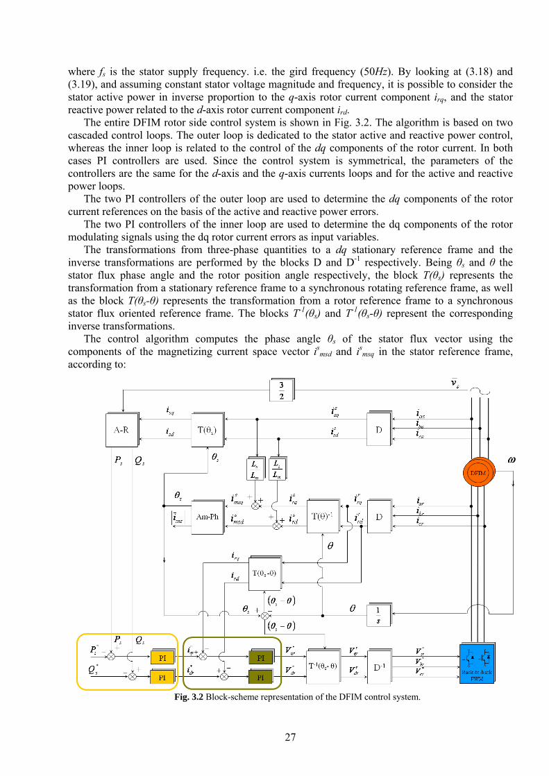
The entire DFIM rotor side control system is shown in Fig. 3.2. The algorithm is based on two cascaded control loops. The outer loop is dedicated to the stator active and reactive power control, whereas the inner loop is related to the control of the dq components of the rotor current. In both cases PI controllers are used. Since the control system is symmetrical, the parameters of the controllers are the same for the d-axis and the q-axis currents loops and for the active and reactive power loops.
The two PI controllers of the outer loop are used to determine the dq components of the rotor current references on the basis of the active and reactive power errors.
The two PI controllers of the inner loop are used to determine the dq components of the rotor modulating signals using the dq rotor current errors as input variables.
The transformations from three-phase quantities to a dq stationary reference frame and the inverse transformations are performed by the blocks D and D-1 respectively. Being θs and θ the stator flux phase angle and the rotor position angle respectively, the block T(θs) represents the transformation from a stationary reference frame to a synchronous rotating reference frame, as well as the block T(θs-θ) represents the transformation from a rotor reference frame to a synchronous stator flux oriented reference frame. The blocks T-1(θs) and T-1(θs-θ) represent the corresponding inverse transformations.
The control algorithm computes the phase angle θs of the stator flux vector using the components of the magnetizing current space vector is
msd and ismsq in the stator reference frame,
according to:
Fig. 3.2 Block-scheme representation of the DFIM control system.
28
⎟⎟⎠
⎞⎜⎜⎝
⎛= s
msd
smsq
s ii
arctanθ . (3.20)
In order to increase the accuracy in the computation of the phase angle θs, a complex digital
filter is applied to isolate the fundamental frequency component of the magnetizing current space vector s
msi . An alternative solution would be the utilization of a Phase Locked Loop (PLL) system in order to track the fundamental phase angle. Such a solution will be presented in the next paragraph where the grid side control of the back to back converter is discussed. The complex digital filter was preferred since it allows to extract not only the phase angle but also the magnitude of the magnetizing current space vector that is used for the dynamic emf compensation in the q-axis rotor current loop. The transfer function of the digital filter in terms of Laplace transform is derived hereafter.
In the synchronous reference frame which rotates at a constant angular speed 2πfs, the filtered magnetizing current vector )( filmsi is obtained by applying a first order low-pass filter to the magnetizing current vector msi yielding:
msfilms is
iτ+
=1
1)( . (3.21)
where τ is the low-pass filter time constant.
The magnetizing current vector in the synchronous reference frame is related to the magnetizing current vector in the stationary reference frame by the following relationship:
sjs
msms eii θ−= (3.22) By substituting (3.22) in (3.21), the equation of the filtered magnetizing current vector in the
stationary reference frame becomes:
sms
s
sfilms i
ji
τωτ −+=
s11
)( . (3.23)
where ωs is the stator flux angular frequency, assumed constant and equal to 2πfs [rad/s], i.e. the grid angular frequency. Then the dq components of the magnetizing current vector can be derived from (3.23), yielding:
( )( ) 222)( s1
s1τωττωτ
s
smsqs
smsds
filmsd
iii
++
−+= . (3.24)
( )
( ) 222)( s1s1τωτ
ττω
s
smsq
smsdss
filmsq
iii
++
++= . (3.25)
Equations (3.24),(3.25) and (3.20) are implemented in the block named “Am-Ph” in the control
scheme of Fig. 3.2. It’s worth underlining that an Euler discretization for (3.24),(3.25) may lead to unstable behavior of the complex digital filter for high value of the time constant τ. To overcome this limitation a discretization based on a second order Taylor series expansion has been adopted to make the filter stable for all the time constant values of interest.

29
Finally the block “A-R” of Fig. 3.2 calculates the stator active and reactive power by using (3.16) and (3.17).
Once the relationship between stator and rotor dq current components in the stator flux oriented reference frame has been found, it’s possible to express rotor fluxes and voltages as a function of solely rotor currents.
In fact by substituting (3.14), (3.15) in (3.7) and (3.8) the following expression for the dq rotor fluxes can be retrieved:
sm
s
s
mrdrrd L
vLLiL
ωσϕ
2
+= . (3.26)
rqrrq iLσϕ = . (3.27)
where σ is the well known leakage factor expressed as:
rs
mrs
LLLLL 2−
=σ . (3.28)
The rotor voltages as a function of the rotor currents can be obtained by substituting (3.14),
(3.15), (3.26) and (3.27) in (3.3) and (3.4):
rqrsrd
rrdrrd iLdt
diLiRv σωωσ )( −−+= . (3.29)
sm
s
s
msrdrs
rqrrqrrq L
vLLiL
dtdi
LiRvω
ωωσωωσ2
)()( −+−++= . (3.30)
These two equations are used for the design of rotor currents PI controllers as will be shown in
the next chapter. If steady state operation is assumed and the rotor active power is computed through the following expression:
( )rqrqrdrdr ivivP +=23 . (3.31)
combining (3.29), (3.30) and (3.31) leads to:
( ) rqsm
s
s
msrqrrdrr i
Lv
LLiRiRP
ωωω
222 )(
23
23
−++= . (3.32)
Finally introducing in the last term at the right end side the relation between the rotor and stator
q current components as in (3.15) we find the following expression relating stator and rotor active power under the hypothesis of negligible stator resistances:
( ) srqrrdrr sPiRiRP −+= 22
23 . (3.33)
being:
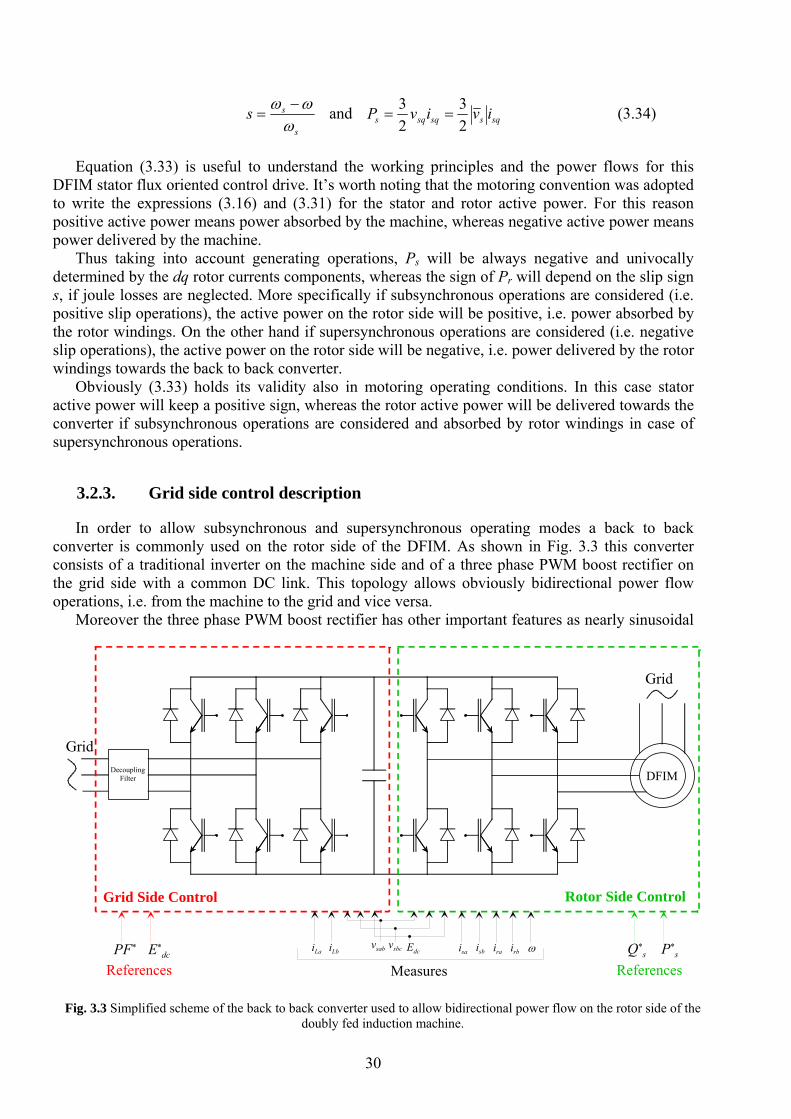
30
s
ssω
ωω −= and sqssqsqs ivivP
23
23
== (3.34)
Equation (3.33) is useful to understand the working principles and the power flows for this
DFIM stator flux oriented control drive. It’s worth noting that the motoring convention was adopted to write the expressions (3.16) and (3.31) for the stator and rotor active power. For this reason positive active power means power absorbed by the machine, whereas negative active power means power delivered by the machine.
Thus taking into account generating operations, Ps will be always negative and univocally determined by the dq rotor currents components, whereas the sign of Pr will depend on the slip sign s, if joule losses are neglected. More specifically if subsynchronous operations are considered (i.e. positive slip operations), the active power on the rotor side will be positive, i.e. power absorbed by the rotor windings. On the other hand if supersynchronous operations are considered (i.e. negative slip operations), the active power on the rotor side will be negative, i.e. power delivered by the rotor windings towards the back to back converter.
Obviously (3.33) holds its validity also in motoring operating conditions. In this case stator active power will keep a positive sign, whereas the rotor active power will be delivered towards the converter if subsynchronous operations are considered and absorbed by rotor windings in case of supersynchronous operations.
3.2.3. Grid side control description
In order to allow subsynchronous and supersynchronous operating modes a back to back converter is commonly used on the rotor side of the DFIM. As shown in Fig. 3.3 this converter consists of a traditional inverter on the machine side and of a three phase PWM boost rectifier on the grid side with a common DC link. This topology allows obviously bidirectional power flow operations, i.e. from the machine to the grid and vice versa.
Moreover the three phase PWM boost rectifier has other important features as nearly sinusoidal
DFIMDecouplingFilter
Grid
Grid
Rotor Side ControlGrid Side Control
vsab vsbc Edc isa isb ira irb ωiLa iLb
MeasuresE*
dcPF* P*sQ*
s
References References
Fig. 3.3 Simplified scheme of the back to back converter used to allow bidirectional power flow on the rotor side of the doubly fed induction machine.
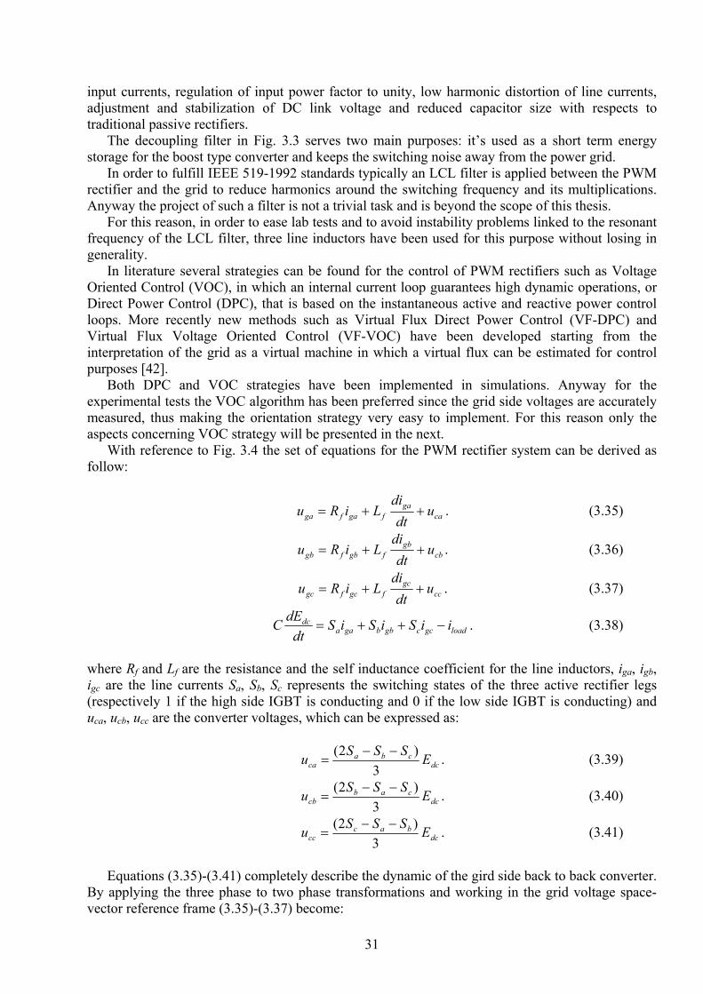
31
input currents, regulation of input power factor to unity, low harmonic distortion of line currents, adjustment and stabilization of DC link voltage and reduced capacitor size with respects to traditional passive rectifiers.
The decoupling filter in Fig. 3.3 serves two main purposes: it’s used as a short term energy storage for the boost type converter and keeps the switching noise away from the power grid.
In order to fulfill IEEE 519-1992 standards typically an LCL filter is applied between the PWM rectifier and the grid to reduce harmonics around the switching frequency and its multiplications. Anyway the project of such a filter is not a trivial task and is beyond the scope of this thesis.
For this reason, in order to ease lab tests and to avoid instability problems linked to the resonant frequency of the LCL filter, three line inductors have been used for this purpose without losing in generality.
In literature several strategies can be found for the control of PWM rectifiers such as Voltage Oriented Control (VOC), in which an internal current loop guarantees high dynamic operations, or Direct Power Control (DPC), that is based on the instantaneous active and reactive power control loops. More recently new methods such as Virtual Flux Direct Power Control (VF-DPC) and Virtual Flux Voltage Oriented Control (VF-VOC) have been developed starting from the interpretation of the grid as a virtual machine in which a virtual flux can be estimated for control purposes [42].
Both DPC and VOC strategies have been implemented in simulations. Anyway for the experimental tests the VOC algorithm has been preferred since the grid side voltages are accurately measured, thus making the orientation strategy very easy to implement. For this reason only the aspects concerning VOC strategy will be presented in the next.
With reference to Fig. 3.4 the set of equations for the PWM rectifier system can be derived as follow:
caga
fgafga udt
diLiRu ++= . (3.35)
cbgb
fgbfgb udt
diLiRu ++= . (3.36)
ccgc
fgcfgc udt
diLiRu ++= . (3.37)
loadgccgbbgaadc iiSiSiS
dtdEC −++= . (3.38)
where Rf and Lf are the resistance and the self inductance coefficient for the line inductors, iga, igb, igc are the line currents Sa, Sb, Sc represents the switching states of the three active rectifier legs (respectively 1 if the high side IGBT is conducting and 0 if the low side IGBT is conducting) and uca, ucb, ucc are the converter voltages, which can be expressed as:
dccba
ca ESSSu3
)2( −−= . (3.39)
dccab
cb ESSSu3
)2( −−= . (3.40)
dcbac
cc ESSSu3
)2( −−= . (3.41)
Equations (3.35)-(3.41) completely describe the dynamic of the gird side back to back converter.
By applying the three phase to two phase transformations and working in the grid voltage space-vector reference frame (3.35)-(3.37) become:
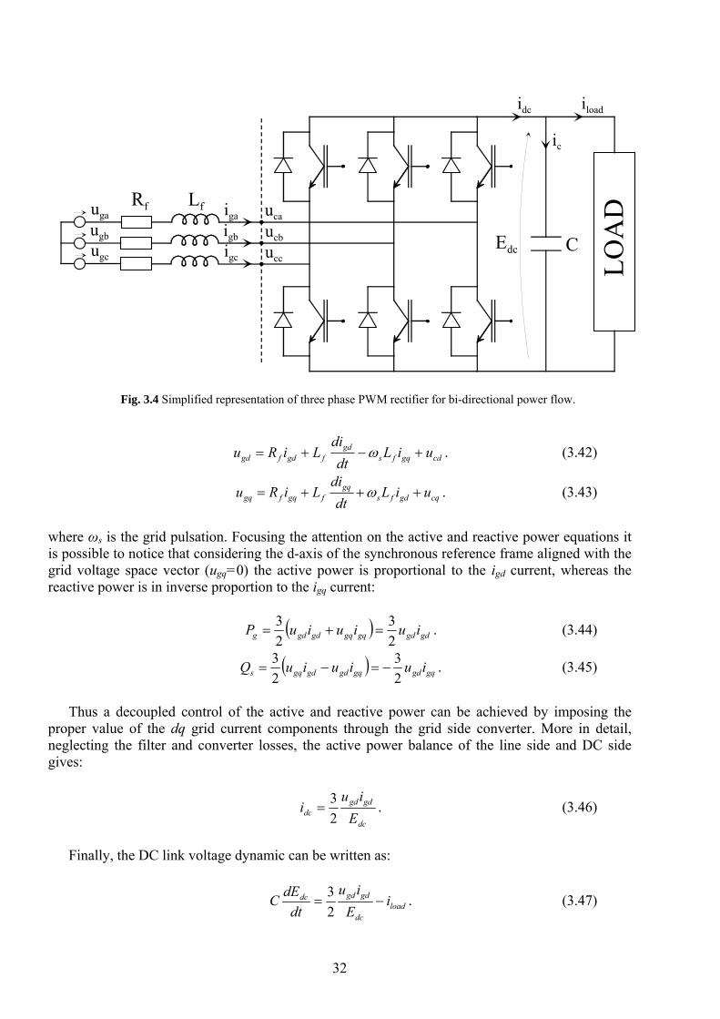
32
cdgqfsgd
fgdfgd uiLdt
diLiRu +−+= ω . (3.42)
cqgdfsgq
fgqfgq uiLdt
diLiRu +++= ω . (3.43)
where ωs is the grid pulsation. Focusing the attention on the active and reactive power equations it is possible to notice that considering the d-axis of the synchronous reference frame aligned with the grid voltage space vector (ugq=0) the active power is proportional to the igd current, whereas the reactive power is in inverse proportion to the igq current:
( ) gdgdgqgqgdgdg iuiuiuP23
23
=+= . (3.44)
( ) gqgdgqgdgdgqs iuiuiuQ23
23
−=−= . (3.45)
Thus a decoupled control of the active and reactive power can be achieved by imposing the
proper value of the dq grid current components through the grid side converter. More in detail, neglecting the filter and converter losses, the active power balance of the line side and DC side gives:
dc
gdgddc E
iui
23
= . (3.46)
Finally, the DC link voltage dynamic can be written as:
loaddc
gdgddc iE
iudt
dEC −=23 . (3.47)
LOA
D
Edc
LfRf
C
uga
ugb
ugc
uca
ucb
ucc
iga
igb
igc
iload
ic
idc
Fig. 3.4 Simplified representation of three phase PWM rectifier for bi-directional power flow.
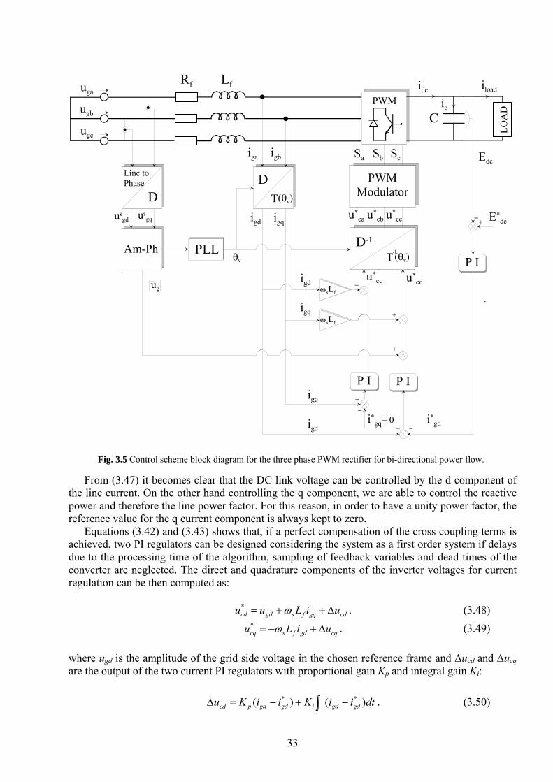
33
From (3.47) it becomes clear that the DC link voltage can be controlled by the d component of the line current. On the other hand controlling the q component, we are able to control the reactive power and therefore the line power factor. For this reason, in order to have a unity power factor, the reference value for the q current component is always kept to zero.
Equations (3.42) and (3.43) shows that, if a perfect compensation of the cross coupling terms is achieved, two PI regulators can be designed considering the system as a first order system if delays due to the processing time of the algorithm, sampling of feedback variables and dead times of the converter are neglected. The direct and quadrature components of the inverter voltages for current regulation can be then computed as:
cdgqfsgdcd uiLuu Δ++= ω* . (3.48)
cqgdfscq uiLu Δ+−= ω* . (3.49)
where ugd is the amplitude of the grid side voltage in the chosen reference frame and Δucd and Δucq are the output of the two current PI regulators with proportional gain Kp and integral gain Ki:
∫ −+−=Δ dtiiKiiKu gdgdigdgdpcd )()( ** . (3.50)
LOA
D
Edc
LfRf
C
uga
ugb
ugc
usgq
iga igb
i*gd
iloadidc
PWM
D
Line toPhase
usgd
Am-Ph
DT(θ )v
PLL
PWMModulator
Sa Sb Sc
D-1
T (θ )v-1
u*ca u*
cb u*cc E*
dc+
-
P I
P I P I
θv
ωsLf
ωsLfug
+
+
igd igq
igd
igq
i*gq= 0
igq
igdu*
cq u*cd
+
+
ic
Fig. 3.5 Control scheme block diagram for the three phase PWM rectifier for bi-directional power flow.
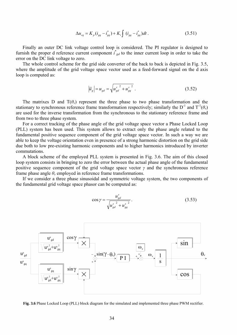
34
∫ −+−=Δ dtiiKiiKu gqgqigqgqpcq )()( ** . (3.51)
Finally an outer DC link voltage control loop is considered. The PI regulator is designed to
furnish the proper d reference current component i*gd to the inner current loop in order to take the
error on the DC link voltage to zero. The whole control scheme for the grid side converter of the back to back is depicted in Fig. 3.5,
where the amplitude of the grid voltage space vector used as a feed-forward signal on the d axis loop is computed as:
22 s
gqsgdgdg uuuu +== . (3.52)
The matrixes D and T(θv) represent the three phase to two phase transformation and the
stationary to synchronous reference frame transformation respectively; similarly the D-1 and T-1(θv) are used for the inverse transformation from the synchronous to the stationary reference frame and from two to three phase system.
For a correct tracking of the phase angle of the grid voltage space vector a Phase Locked Loop (PLL) system has been used. This system allows to extract only the phase angle related to the fundamental positive sequence component of the grid voltage space vector. In such a way we are able to keep the voltage orientation even in presence of a strong harmonic distortion on the grid side due both to low pre-existing harmonic components and to higher harmonics introduced by inverter commutations.
A block scheme of the employed PLL system is presented in Fig. 3.6. The aim of this closed loop system consists in bringing to zero the error between the actual phase angle of the fundamental positive sequence component of the grid voltage space vector γ and the synchronous reference frame phase angle θv employed in reference frame transformations.
If we consider a three phase sinusoidal and symmetric voltage system, the two components of the fundamental grid voltage space phasor can be computed as:
22
cossgq
sgd
sgd
uu
u
+=γ . (3.53)
usgq
P Iθv
usgd
usgd+us
gq2 2
usgq
usgd+us
gq2 2
usgd
+
cos
sin( ++
ωs
1s
sin
cos
γ
sinγ
γ ) θvωv
Fig. 3.6 Phase Locked Loop (PLL) block diagram for the simulated and implemented three phase PWM rectifier.

35
22
sinsgq
sgd
sgq
uu
u
+=γ . (3.54)
Subsequently (3.53) and (3.54) are multiplied by the two components of the space phasor used
for reference frame transformations as follow: )sin(cossincossin vvv θγγθθγ −=− (3.55) Thus the input of the PI regulator is the sine of the error between the two phase angles, whereas
its output is the pulsation of θv(t), whose variation allows to bring the error to zero. For this purpose such a pulsation ωv is integrated and its sine and cosine trigonometric functions are used as feedback signals.
During the initial locking phase the input of the PI regulator (3.55) will obviously assumes both positive and negative values. Assuming that θv(t) is lagging behind the fundamental voltage phase angle γ, there will be a time interval in which the PI regulator will increase the pulsation ωv (for positive values of the sine of the error) making it closer to the pulsation of the input grid voltage space phasor. Then, for negative values of the sine of the error, there will be a shorter time interval in which the PI regulator will decrease the pulsation ωv, thus increasing the difference between such a pulsation and the fundamental pulsation of the grid voltage space phasor.
This asymmetry in time between the positive and negative half wave of the sine of the error produces a positive mean value in the input signal of the PI regulator and therefore a periodic increase of the pulsation ωv until the output angle θv(t) perfectly tracks the fundamental grid voltage phase angle γ with zero steady state error.
In operating conditions close to synchronization the error between the two phase angles γ and θv is small and close to zero so that the input of the PI regulator can be approximated to:
δθγ ≅− )sin( v with vθγδ −= (3.56) With such approximation the PLL system can be considered to have a linear phase detector, i.e.
an input signal to the PI regulator proportional to the difference between the fundamental component phase angle of the grid voltage and the synchronous reference frame phase angle employed in reference frame transformations.
Typically the design of the PI regulator parameters is performed making reference to the linear approximated system presented in Fig. 3.7. The feed forward open loop transfer function has two poles at the origin. Consequently the steady state error to a ramp input will be zero as requested to a PLL system.
On the other hand, the closed loop system is a simple second order system with one zero and two poles. The choice of the proportional and integral gains (Kp and Ki respectively) has to be a
θv+ 1
s
γ θvωvKisKp+
δ=γ
θv
Fig. 3.7 Linearzied PLL block diagram for the design of PI regulator parameters.
36
compromise between a fast dynamic response during the locking phase and a limited bandwidth of the system in order to filter higher order harmonics present in the grid voltage space vector.
Such a bandwidth has been chosen in order to damp the effect of an inverse sequence on the grid voltage consisting in a disturbance on the input signal at a pulsation of 2ωs. Once the system is designed to damp the effect of an inverse sequence, it is consequently able to filter all the higher order harmonics usually present on the grid voltage.
3.3. Railway Traction Systems
3.3.1. Introduction
The research work and the techniques developed for the diagnosis of rotor faults in induction motors for railway traction applications have been carried on in cooperation with a company that designs and realizes railway systems within a European project. For this reason the description of the control system is not detailed as it is secured by non disclosure agreements.
In the following only the aspects of the control algorithm that have a certain impact on the diagnostic procedures will be underlined.
The actual control system is a variable structure control system. In fact the system can switch between different strategies depending on the demand of the driver and on different electrical variables. In order to prove the feasibility of the developed diagnostic techniques for the diagnosis of rotor faults in time varying conditions, such a system has been implemented in simulations for a 400 kW squirrel cage induction motor. In this way a qualitative analysis of the potential performance of the proposed diagnostic methods in a real application has been performed.
Subsequently simulations and experiments have been made with a scaled prototype of the machine and control architecture. For this purpose a “classical” rotor flux direct Field-Oriented control scheme, very close to the one really implemented on a train for a wide range of speeds, has been employed. The most important features of the actual control algorithm and especially those that could affect the developed diagnostic procedures have been implemented trying to reproduce the transient behaviour of the real traction drive.
3.3.2. Railway traction drive
In railways application typically locomotives or motor cars are moved by multiple motors placed on the axles of one boogie. State-of-the-art solutions are based on drives that include a voltage source inverter (VSI) feeding an induction motor or a permanent magnet synchronous motor. However old fashion solutions based on current source inverter (CSI) or on thyristors are still employed, whereas old schemes based on DC series motor or Direct DC motors are no longer employed.
The basic components for a railway traction drive, common to various design solutions are represented in Fig. 3.8. The current is collected either by the pantograph mounted on the top of the train through the contact with the catenary line or through the contact of a third feeder rail and a shoe placed beside the boogie. This second solution is common in metro tunnels, for some mountain tracks and in general for DC supply voltages under 1200V.
Usually more than one pantograph is present on a single locomotive or motor car because of the inhomogeneous railway network electrification which in Europe is highly fragmented and presents the following levels of supply voltage:
• 1.5 kV DC
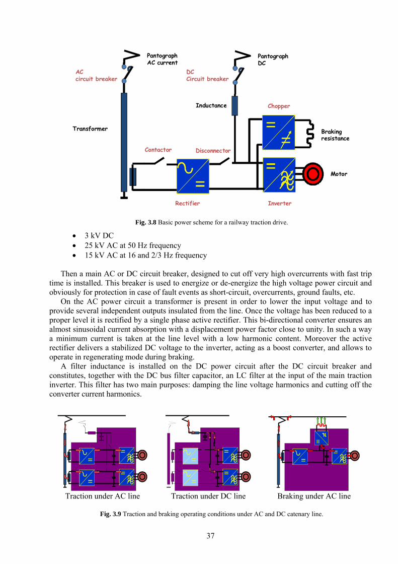
37
• 3 kV DC • 25 kV AC at 50 Hz frequency • 15 kV AC at 16 and 2/3 Hz frequency
Then a main AC or DC circuit breaker, designed to cut off very high overcurrents with fast trip
time is installed. This breaker is used to energize or de-energize the high voltage power circuit and obviously for protection in case of fault events as short-circuit, overcurrents, ground faults, etc.
On the AC power circuit a transformer is present in order to lower the input voltage and to provide several independent outputs insulated from the line. Once the voltage has been reduced to a proper level it is rectified by a single phase active rectifier. This bi-directional converter ensures an almost sinusoidal current absorption with a displacement power factor close to unity. In such a way a minimum current is taken at the line level with a low harmonic content. Moreover the active rectifier delivers a stabilized DC voltage to the inverter, acting as a boost converter, and allows to operate in regenerating mode during braking.
A filter inductance is installed on the DC power circuit after the DC circuit breaker and constitutes, together with the DC bus filter capacitor, an LC filter at the input of the main traction inverter. This filter has two main purposes: damping the line voltage harmonics and cutting off the converter current harmonics.
Inverter
Motor
Chopper
Brakingresistance
Transformer
PantographAC current
Rectifier
Contactor Disconnector
AC circuit breaker
PantographDC
DCCircuit breaker
Inductance
Fig. 3.8 Basic power scheme for a railway traction drive.
Traction under AC line Traction under DC line Braking under AC line
Fig. 3.9 Traction and braking operating conditions under AC and DC catenary line.
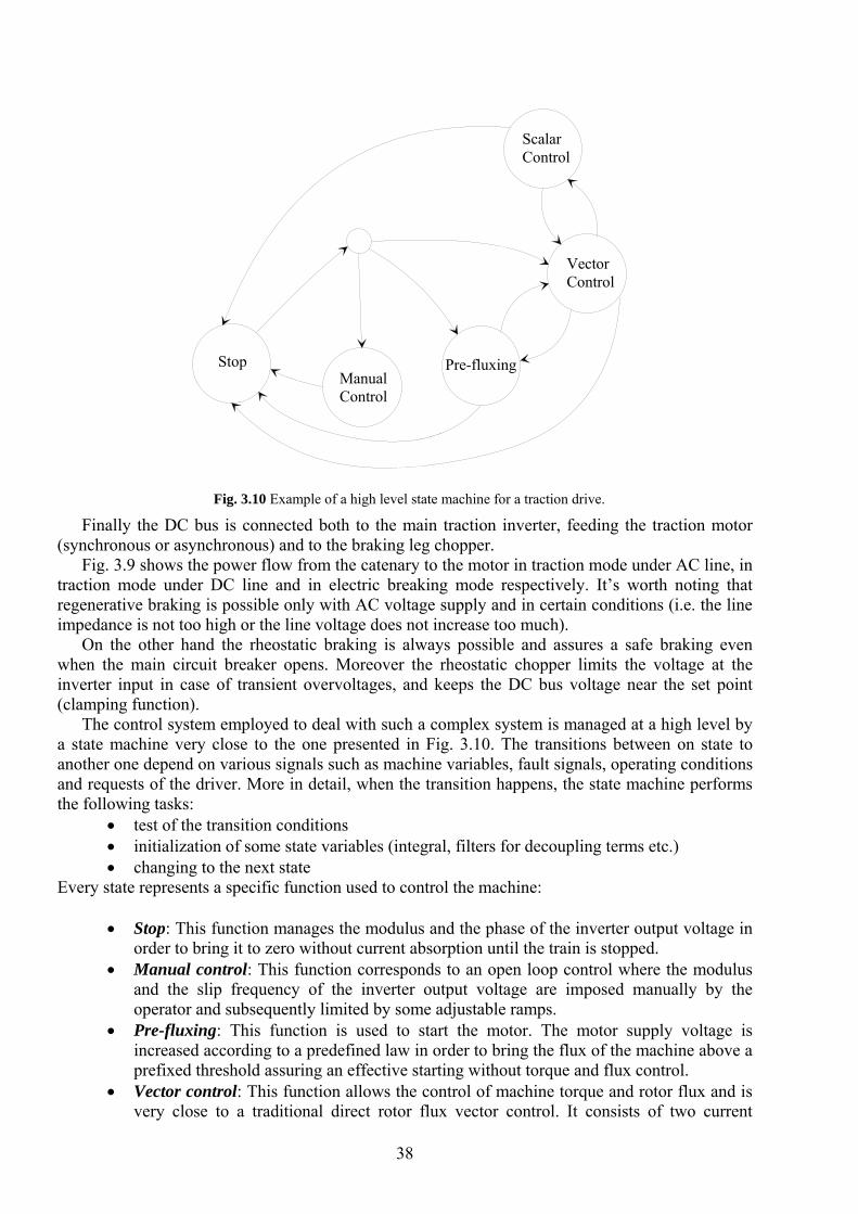
38
Finally the DC bus is connected both to the main traction inverter, feeding the traction motor (synchronous or asynchronous) and to the braking leg chopper.
Fig. 3.9 shows the power flow from the catenary to the motor in traction mode under AC line, in traction mode under DC line and in electric breaking mode respectively. It’s worth noting that regenerative braking is possible only with AC voltage supply and in certain conditions (i.e. the line impedance is not too high or the line voltage does not increase too much).
On the other hand the rheostatic braking is always possible and assures a safe braking even when the main circuit breaker opens. Moreover the rheostatic chopper limits the voltage at the inverter input in case of transient overvoltages, and keeps the DC bus voltage near the set point (clamping function).
The control system employed to deal with such a complex system is managed at a high level by a state machine very close to the one presented in Fig. 3.10. The transitions between on state to another one depend on various signals such as machine variables, fault signals, operating conditions and requests of the driver. More in detail, when the transition happens, the state machine performs the following tasks:
• test of the transition conditions • initialization of some state variables (integral, filters for decoupling terms etc.) • changing to the next state
Every state represents a specific function used to control the machine:
• Stop: This function manages the modulus and the phase of the inverter output voltage in order to bring it to zero without current absorption until the train is stopped.
• Manual control: This function corresponds to an open loop control where the modulus and the slip frequency of the inverter output voltage are imposed manually by the operator and subsequently limited by some adjustable ramps.
• Pre-fluxing: This function is used to start the motor. The motor supply voltage is increased according to a predefined law in order to bring the flux of the machine above a prefixed threshold assuring an effective starting without torque and flux control.
• Vector control: This function allows the control of machine torque and rotor flux and is very close to a traditional direct rotor flux vector control. It consists of two current
StopManualControl
Pre-fluxing
VectorControl
ScalarControl
Fig. 3.10 Example of a high level state machine for a traction drive.
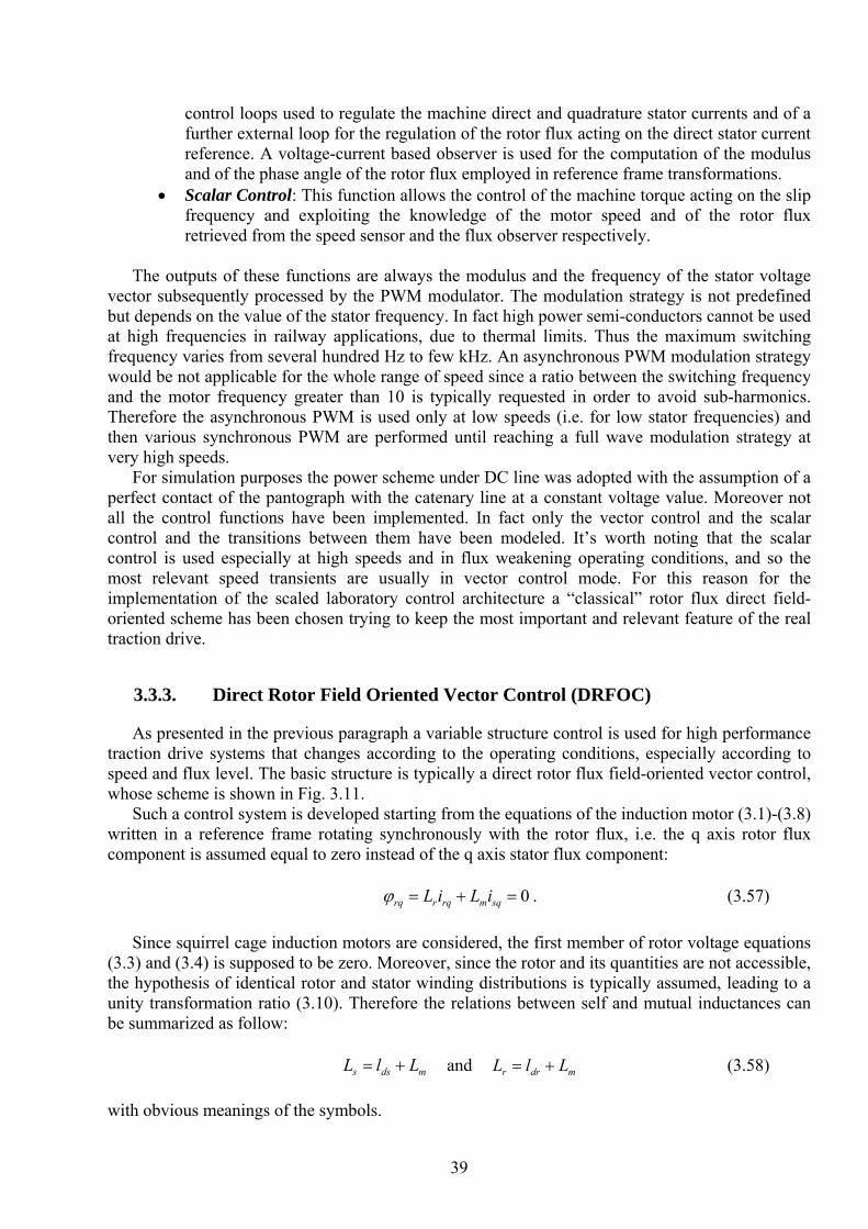
39
control loops used to regulate the machine direct and quadrature stator currents and of a further external loop for the regulation of the rotor flux acting on the direct stator current reference. A voltage-current based observer is used for the computation of the modulus and of the phase angle of the rotor flux employed in reference frame transformations.
• Scalar Control: This function allows the control of the machine torque acting on the slip frequency and exploiting the knowledge of the motor speed and of the rotor flux retrieved from the speed sensor and the flux observer respectively.
The outputs of these functions are always the modulus and the frequency of the stator voltage
vector subsequently processed by the PWM modulator. The modulation strategy is not predefined but depends on the value of the stator frequency. In fact high power semi-conductors cannot be used at high frequencies in railway applications, due to thermal limits. Thus the maximum switching frequency varies from several hundred Hz to few kHz. An asynchronous PWM modulation strategy would be not applicable for the whole range of speed since a ratio between the switching frequency and the motor frequency greater than 10 is typically requested in order to avoid sub-harmonics. Therefore the asynchronous PWM is used only at low speeds (i.e. for low stator frequencies) and then various synchronous PWM are performed until reaching a full wave modulation strategy at very high speeds.
For simulation purposes the power scheme under DC line was adopted with the assumption of a perfect contact of the pantograph with the catenary line at a constant voltage value. Moreover not all the control functions have been implemented. In fact only the vector control and the scalar control and the transitions between them have been modeled. It’s worth noting that the scalar control is used especially at high speeds and in flux weakening operating conditions, and so the most relevant speed transients are usually in vector control mode. For this reason for the implementation of the scaled laboratory control architecture a “classical” rotor flux direct field-oriented scheme has been chosen trying to keep the most important and relevant feature of the real traction drive.
3.3.3. Direct Rotor Field Oriented Vector Control (DRFOC)
As presented in the previous paragraph a variable structure control is used for high performance traction drive systems that changes according to the operating conditions, especially according to speed and flux level. The basic structure is typically a direct rotor flux field-oriented vector control, whose scheme is shown in Fig. 3.11.
Such a control system is developed starting from the equations of the induction motor (3.1)-(3.8) written in a reference frame rotating synchronously with the rotor flux, i.e. the q axis rotor flux component is assumed equal to zero instead of the q axis stator flux component:
0=+= sqmrqrrq iLiLϕ . (3.57) Since squirrel cage induction motors are considered, the first member of rotor voltage equations
(3.3) and (3.4) is supposed to be zero. Moreover, since the rotor and its quantities are not accessible, the hypothesis of identical rotor and stator winding distributions is typically assumed, leading to a unity transformation ratio (3.10). Therefore the relations between self and mutual inductances can be summarized as follow:
mdss LlL += and mdrr LlL += (3.58)
with obvious meanings of the symbols.
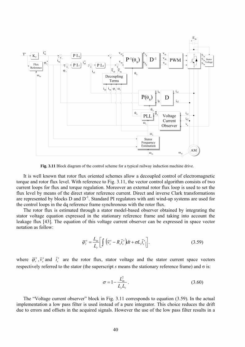
40
It is well known that rotor flux oriented schemes allow a decoupled control of electromagnetic torque and rotor flux level. With reference to Fig. 3.11, the vector control algorithm consists of two current loops for flux and torque regulation. Moreover an external rotor flux loop is used to set the flux level by means of the direct stator reference current. Direct and inverse Clark transformations are represented by blocks D and D-1. Standard PI regulators with anti wind-up systems are used for the control loops in the dq reference frame synchronous with the rotor flux.
The rotor flux is estimated through a stator model-based observer obtained by integrating the stator voltage equation expressed in the stationary reference frame and taking into account the leakage flux [43]. The equation of this voltage current observer can be expressed in space vector notation as follow:
( ) ⎥⎦⎤
⎢⎣⎡ +−= ∫ s
sss
ssss
r
msr iLdtiRv
LL σϕ . (3.59)
where s
rϕ , ssv and s
si are the rotor flux, stator voltage and the stator current space vectors respectively referred to the stator (the superscript s means the stationary reference frame) and σ is:
rs
m
LLL2
1−=σ . (3.60)
The “Voltage current observer” block in Fig. 3.11 corresponds to equation (3.59). In the actual
implementation a low pass filter is used instead of a pure integrator. This choice reduces the drift due to errors and offsets in the acquired signals. However the use of the low pass filter results in a
AM
VoltageCurrent
Observer
DecouplingTerms
KT
FluxReference
T* isq
isd
+ -
+ -isd
isq
θ
ωm
+ -
vsd
vsq
Edc
ϕ r*
s
ϕ r
is1
s2i
S1
S2
S3
sv
StatorVoltage
PLL
StatorFrequencyEstimation
D
D-1
ωs
ωm
vα
vβ
vsa
vsb
vsc
iα
iβ
*
*
ωs
is1
s2i
ωs
PWM
ϕ r
P I dP I f
P I q
isd isq
ωm
θs
θs˜
θs
P-1(θs)
P(θs)
vsd˜ vsq˜
Fig. 3.11 Block diagram of the control scheme for a typical railway induction machine drive.
41
wrong computation of the rotor flux space vector in terms of magnitude and phase angle. An estimate of the stator pulsation is used to compensate these errors:
mr
sq
r
mrs p
iLLR ω
ϕω += *
*
ˆ . (3.61)
where ωm is the measured mechanical speed, p is the pole pairs number, i*
sq is the reference value of the q axis stator current and φ*
r is the reference value of the rotor flux. Relationship (3.61) is represented in Fig. 3.11 by the “Stator Frequency Estimation” block and can be easily retrieved form (3.4) considering the rotor flux orientation expressed in (3.57). Reference values are used instead of measured and estimated machine variables.
As stated before this stator frequency estimate is used to compensate errors in the magnitude and phase angle of the rotor flux caused by the low pass filter used for the integration. The phase angle correction is performed inside the PLL block used also to filter undesired harmonic noise, thus allowing a perfect tracking of the compensated rotor flux phase angle. The output of the PLL block is then used in the reference frame matrix transformations P(θs) and P-1(θs).
On the other hand the compensated rotor flux magnitude is used inside the “Decoupling Terms” block together with the relationship (3.61) and the measured currents in the synchronous reference frame to compute the dynamic back-emf compensation terms:
sqssd iLv σω~ −= . (3.62)
⎟⎟⎠
⎞⎜⎜⎝
⎛+= r
r
msdssq L
LiLv ϕσω~ . (3.63)
The compensated magnitude of the estimated rotor flux φr is eventually used as feedback signal
for the outer loop. The value of the reference quadrature stator current is obtained from the reference torque and
reference flux signal through the following equation:
*
**
rTq
TKiϕ
= with m
rT pL
LK32
= (3.64)
where T* is the reference torque. On the other hand the reference flux is obtained on the basis of the nominal values for torque and rotor flux as follow:
rnomnon
r TT ϕϕ
** = . (3.65)
This choice keeps the slip frequency quite constant. In fact the torque in case of rotor flux
orientation can be expressed as:
2
23
rr
r
RpT ϕω
= . (3.66)
where ωr=(ωs-ω) is the slip angular frequency. Thus by substituting (3.65) in (3.66) and considering reference values, the constant slip frequency assumes the value:
42
p
RT r
rnom
nomr 23
2ϕ
ω = . (3.67)
This choice for the reference flux provides a better robustness of the control system against
speed errors and reduces the losses at low torque. The rotor flux nominal value is computed according to motor nameplate data and machine
parameters as follow:
snom
nomsnom
r
rmnomsnom
smrnom f
IRV
RLpf
LLπσωπ
ϕ2
)(2)2(1
2
−
⎟⎟⎠
⎞⎜⎜⎝
⎛ −+
= . (3.68)
The control system as presented in Fig. 3.11, is not able to deliver torque at very low speed. For
this reason another rotor flux observer has been implemented in order to allow operations at zero speed. This choice can be considered as an alternative to the open loop operations.
The implemented rotor flux observer is based on the measured electrical speed ω=pωm and on measured stator currents. The differential equation on which such observer is based can be easily retrieved from the rotor voltage equations written in a stationary reference frame taking into account the rotor flux equations:
srq
srds
rdr dtdiR ωϕϕ
++=0 . (3.69)
srd
srqs
rqr dtd
iR ωϕϕ
++=0 . (3.70)
ssdm
srdr
srd iLiL +=ϕ . (3.71)
ssqm
srqr
srq iLiL +=ϕ . (3.72)
By substituting (3.71), (3.72) in (3.69), (3.70) and considering the rotor flux as a state variable,
its two components in the stationary reference frame can be computed by integrating the following equations:
ssd
r
msrq
srd
r
srd iL
dtd
τωϕϕ
τϕ
+−−=1 . (3.73)
ssq
r
msrd
srq
r
srq iL
dtd
τωϕϕ
τϕ
++−=1 . (3.74)
where τr=Lr/Rr is the rotor time constant. This speed current observer is effective and presents its best performances at low speeds. As stated before it is used only for starting operations. Above a prefixed threshold speed the rotor flux estimate is smoothly switched from the speed-current observer to the voltage-current one based on (3.59). All the simulation and experimental results presented in this thesis have been performed relying on the latter observer.
It’s worth noting that an Euler discretization for (3.73) and (3.74) may lead to unstable behavior at high speed. To overcome this limitation a discretization based on a second order Taylor series expansion has been adopted to make the observer stable for the whole speed range of interest.
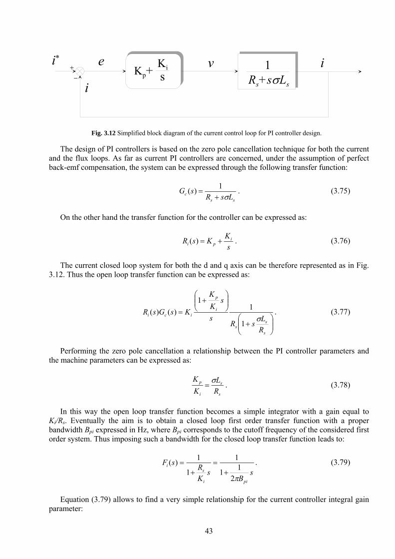
43
The design of PI controllers is based on the zero pole cancellation technique for both the current and the flux loops. As far as current PI controllers are concerned, under the assumption of perfect back-emf compensation, the system can be expressed through the following transfer function:
ss
c LsRsG
σ+=
1)( . (3.75)
On the other hand the transfer function for the controller can be expressed as:
s
KKsR ipi +=)( . (3.76)
The current closed loop system for both the d and q axis can be therefore represented as in Fig.
3.12. Thus the open loop transfer function can be expressed as:
⎟⎟⎠
⎞⎜⎜⎝
⎛+
⎟⎟⎠
⎞⎜⎜⎝
⎛+
=
s
ss
i
p
ici
RLsR
s
sKK
KsGsRσ1
11
)()( . (3.77)
Performing the zero pole cancellation a relationship between the PI controller parameters and
the machine parameters can be expressed as:
s
s
i
p
RL
KK σ
= . (3.78)
In this way the open loop transfer function becomes a simple integrator with a gain equal to
Ki/Rs. Eventually the aim is to obtain a closed loop first order transfer function with a proper bandwidth Bpi expressed in Hz, where Bpi corresponds to the cutoff frequency of the considered first order system. Thus imposing such a bandwidth for the closed loop transfer function leads to:
s
Bs
KRsF
pii
si
π211
1
1
1)(+
=+
= . (3.79)
Equation (3.79) allows to find a very simple relationship for the current controller integral gain
parameter:
+ 1Rs+sσLs
KisKp+
i* e iv
i
Fig. 3.12 Simplified block diagram of the current control loop for PI controller design.
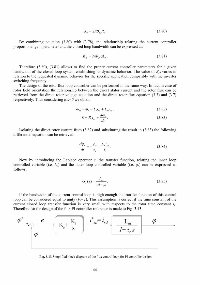
44
spii RBK π2= . (3.80) By combining equation (3.80) with (3.78), the relationship relating the current controller
proportional gain parameter and the closed loop bandwidth can be expressed as: spip LBK σπ2= . (3.81) Therefore (3.80), (3.81) allows to find the proper current controller parameters for a given
bandwidth of the closed loop system establishing its dynamic behavior. The value of Bpi varies in relation to the requested dynamic behavior for the specific application compatibly with the inverter switching frequency.
The design of the rotor flux loop controller can be performed in the same way. In fact in case of rotor field orientation the relationship between the direct stator current and the rotor flux can be retrieved from the direct rotor voltage equation and the direct rotor flux equation (3.3) and (3.7) respectively. Thus considering φrq=0 we obtain:
sdmrdrrrd iLiL +==ϕϕ . (3.82)
dt
diR rrdr
ϕ+=0 . (3.83)
Isolating the direct rotor current from (3.82) and substituting the result in (3.83) the following
differential equation can be retrieved:
r
sdm
r
rr iLdt
dττ
ϕϕ+−= . (3.84)
Now by introducing the Laplace operator s, the transfer function, relating the inner loop
controlled variable (i.e. isd) and the outer loop controlled variable (i.e. φr) can be expressed as follows:
s
LsGr
mf τ+
=1
)( . (3.85)
If the bandwidth of the current control loop is high enough the transfer function of this control
loop can be considered equal to unity (Fi=1). This assumption is correct if the time constant of the current closed loop transfer function is very small with respects to the rotor time constant τr. Therefore for the design of the flux PI controller reference is made to Fig. 3.13
+ Lm
1+τr sKisKp+
ϕ* e i*sd=isd
ϕ
ϕ
Fig. 3.13 Simplified block diagram of the flux control loop for PI controller design.

45
The zero pole cancellation can be performed also in this case, thus leading to the following relationship for the proportional and integral gain parameters:
ri
p
KK
τ= . (3.86)
Now assuming, also for the flux loop, a prefixed value of the closed loop transfer function
bandwidth Bpf the value of the controller parameters can be computed as follow:
s
Bs
LK
sF
pfmi
f
π211
111
1)(+
=+
= . (3.87)
Then by imposing the same time constant for both transfer functions in (3.87) and taking into
account (3.86) the proportional and integral gain values become:
m
rpfp L
BK
τπ2= . (3.88)
m
pfi L
BK
π2= . (3.89)
Typically in a real system the value of the flux loop bandwidth is usually small, in the range of a
few Hertz for low-voltage low-power motors or even less than 1 Hz for high power drives.

46
47
Chapter 4
Diagnostic Techniques
4.1. Introduction
In this chapter the diagnostic techniques developed for squirrel cage induction motors and Doubly Fed Induction Machines (DFIM) based drives are presented. As far as squirrel cage asynchronous motors are concerned, the attention has been focused on rotor failures (i.e. broken bars). The techniques for fault detection and quantification of this fault have been developed for a specific drive used for railway traction applications and then experimentally validated on a scaled laboratory prototype. Rotor faults are not very frequent indeed, however their detection at incipient stage is a key item as their failure sequence is slow. In fact the time evolution from root causes to actual failures (failure sequence) is very different depending on different fault types. If a failure sequence is rapid then effective condition monitoring is impossible and this is the situation for electrical faults detected by protection, where the period of action may be only seconds or cycles of the electrical machine variables. However, if the failure sequence is days, weeks or months, then condition monitoring has the potential to provide early warning of the impending failure.
For rotor faults the failure sequence is days and, if not properly managed, can degenerate into a catastrophic fault, such as stator or mechanical fault. Hence the detection of a rotor fault at an early stage is useful to set up post fault operation that must bring safely the train to the next station, with a suitable reduction of performances.
The techniques developed for the detection and quantification of rotor faults in induction machine based traction drives presented hereafter are:
• Demodulation technique • Virtual Current Technique (VCT)
The first one consists in a time domain procedure that processes the stator currents in order to
isolate a single fault frequency component in a way not dependent on speed and frequency variations.
The second one is a strategy for broken-bar quantification in a way not dependent on the bandwidth of the external flux loop present in the traction drive control system. This strategy is based on the interpretation of a rotor fault as a disturbance on the output of the closed loop traction system.
48
Afterwards stator and rotor phase unbalances have been studied for DFIM employed in wind turbine generators. It is obvious that reliable and secure generation systems are needed since the areas in which they are installed are frequently not accessible. Therefore it is necessary to detect incipient faults as soon as possible to minimize maintenance cost and prevent unscheduled downtimes through advanced on-line diagnostic techniques for electrical and mechanical faults.
Stator and rotor electrical asymmetries have been successfully detected through the following technique:
• Rotor modulating signals signature analysis
The basic idea consists in taking into account the influence of the current loops present in the
control scheme usually employed for the decoupled control of active and reactive stator power. Their influence makes the signature analysis of the stator or rotor currents, usually employed for electrical fault diagnosis in mains supplied machines, less reliable and so other machine variables has to be considered for an effective fault detection. Simulations and experiments revealed that the signature of the rotor modulating signals of the PWM converter and more in general of rotor voltages can be assumed as a good diagnostic index.
Moreover the wavelet transform has been considered and validated as a valuable tool for signature extraction thanks to its capability to give an appropriate resolution both in time and frequency for the considered fault harmonic isolation. Finally the impact of the loop bandwidth on this diagnostic procedure have been evaluated.
4.2. Demodulation Technique
4.2.1. Introduction
On line diagnosis and early detection of faults in induction machines in adjustable speed drives has focused the attention of researchers, since it allows to reduce maintenance costs and down-times.
In some applications, where continuous operation is a key item, such as railway applications, the need for a preventive fault diagnosis is an extremely important point. For example the case of railway applications is investigated in [44], [45] in order to design a traction drive oriented to maximum fault tolerance. In [46], the use of the Vienna Monitoring Method (VMM) is investigated for a traction drive application where rotor fault detection was successfully verified in transient and steady-state conditions.
In this framework, fault detection and the prognosis of rotor faults is critical for industrial applications though rotor faults are only about 10% of the overall induction machine faults [7]. In fact, the breakage of a bar leads to high current in adjacent bars, thus leading to potential further breakage and stator faults as well.
Motor current signature analysis (MCSA) was extensively used to detect broken rotor bar and end ring faults in induction motors [2], [24], [47], [48]. In steady-state conditions, a quite robust diagnostic index is the sum of the amplitudes of the left and right sideband components of the stator current that is independent of inertia and proportional to the number of adjacent broken bars. The main shortcomings of MCSA are its dependence on the machine slip s, speed, and load, though the dependence on load torque variations can be compensated [49]. Moreover, MCSA fails for current controlled drives as the control loop masks the oscillation of the stator current. If an ideal control loop is considered, the controlled variable is desensitized and anomalous lines appear in manipulated variables. In actual conditions, depending on the bandwidth, either the manipulated
49
(voltage) or controlled (current) variable spectrum is more sensitive to the fault. Hence, new diagnostic indexes can be used that are based on control variables [50], [51], [52].
Anyway for the considered traction drive the external flux loop, present in the control architecture, transfers the characteristic rotor fault harmonics at the input of the inner current loop. For this reason the signature of stator currents keeps its sensitivity allowing an effective fault detection.
Other techniques have been investigated for rotor faults besides MCSA or its variants. Several demodulation methods were presented to extract fault information from the current: in [53] envelope analysis, Hilbert transformation, and Park transformation were used to perform amplitude demodulation of rotor faults. Other methods were based on multiple electrical signals such as torque and leakage flux. VMM [29] relies on voltage, current signals, and measured rotor position to check deviations in terms of instantaneous torque obtained by two different machine models. Also, signal injection techniques were proposed, relying on methods similar to those adopted for sensorless drive control [22]. However, typically in traction drive systems, the switching frequency is very low, making the detection of the faults through the signal injection strategy impossible.
Anyway, for time-varying conditions, the most commonly adopted techniques are based on time-frequency analysis. Complex techniques were presented to cope with this issue, including high-frequency resolution methods [54], time-frequency distributions [55], [56], and wavelets [57]–[60]. All the above methods require heavy computation and complex procedures in order to analyze the time-frequency distribution and to retrieve the information related to rotor faults. Though the computation time itself is not an issue provided that data are sampled, stored, and post processed, in industrial applications, the requirement of minimum complexity is a mandatory issue. In fact, with time-frequency analysis, a few major shortcomings appear:
• the latency can be high, and a large memory is required to store the data that will be
processed; • a large number of samples is required in order to achieve reliable results; • specialized hardware could be required.
A simpler method could provide accurate fault detection in time varying conditions even with a
reduced number of samples. Moreover, it can be included in the available firmware used for the drive control, allowing the realization of an effective fault diagnosis at no additional hardware cost.
A typical example of transient behavior is the case of railway traction applications, where torque and speed vary depending on the journey, preventing the use of MCSA and classical spectral analysis. As stated in the previous chapter reference is made to a typical traction drive for railway application systems and to its scaled laboratory prototype; however, the proposed method is general, provided that a similar control architecture is used.
Electric drives for traction applications operate in field weakening mode at the cruise speed. Nevertheless, the most relevant accelerations are usually in the constant torque mode since the load torque is lower, being proportional to the square of the speed. Here, reference is made to time-varying conditions, and thus to constant torque mode.
The issue of rotor fault detection can be solved if a diagnostic index is defined that is independent of slip and stator frequency. Here, a simple demodulation procedure in the time domain is proposed that processes the stator currents, relying on stator frequency and machine slip accurately retrieved by the drive control. After the demodulation process, a component is obtained whose amplitude is related to the rotor fault and whose frequency is constant, independently of the stator frequency and speed.
It’s worth noting that the demodulation technique presented here is applied to stator currents but can also be applied to other variables in order to extract the faulty components.
50
4.2.2. Demodulation of rotor fault signature in time varying conditions
As previously said the basic idea of the developed technique consists in a simple time domain processing technique that exploits already available control signals for the rotor fault diagnosis.
Typically in case of broken bars the amplitude of the left and right sideband components of a phase current are monitored in order to sense their variation in steady state conditions. Anyway traction drive operations require cyclic torque and speed variations. Under the above conditions the sideband components, whose amplitude must be monitored for diagnostic purposes, is spread in frequency. It turns out that the direct application of MCSA to machine stator currents or to control variables is not effective.
A simple solution for an efficient diagnosis of electrical faults of induction machines under non stationary conditions is presented here.
Adjacent broken bars produce an amplitude modulation of the rotor current, whose carrier is sωs, where s is the slip, ωs = 2πfs is the stator pulsation, and fs is the stator frequency. In terms of rotor current space vector this amplitude modulation is the result of an inverse sequence at frequency -sωs. This modulation is reported to the stator quantities at the angular frequency:
sl s ωω )21( −= (4.1)
and, because of the speed ripple effect [25] also at the frequency: sr s ωω )21( += (4.2)
corresponding to the left and right side bands respectively. The whole frequency propagation for a rotor asymmetry due to broken bars have been already reported in the first chapter showing that other harmonics appear around the fundamental at angular frequencies (1-4s)ωs and (1+4s)ωs and so on. Anyway those higher order fault harmonics are usually negligible due to the damping effect of motor and load inertia. If other effects, such as slotting and saturation are neglected, it can be assumed that the major components of a stator phase current are represented by:
)cos()cos()cos()( rrrlllssfs tItItIti ϕωϕωϕω +++++= (4.3)
where If, Il, and Ir represent the amplitudes of the fundamental component, of the left and of the right side band respectively and φs, φl, and φr their phase angles. The same considerations can be done with reference to the stator current space vector expressed as:
⎟⎟⎠
⎞⎜⎜⎝
⎛++= 3
43
2
)()()(32)(
ππ j
sc
j
sbsas etietititi (4.4)
where isa(t), isb(t), and isc(t) are the stator three phase currents. Therefore under the same assumptions it can be considered that the major components of a stator phase current space vector are represented by:
)()()()( rrllss tj
rtj
ltj
fs eieieiti ϕωϕωϕω +++ ++= (4.5) In time-varying conditions, the amplitudes Il and Ir in (4.3) cannot be detected through a
frequency analysis since ωl and ωr are spread across a wide frequency range, making it impossible to detect their amplitude correctly. In fact, the sideband components ωl and ωr vary as a function of time according to machine slip and supply frequency.
51
A simple processing of a stator phase current or of the respective space vector can be made, so that all the information related to the fault is traced back to a single component, whose amplitude is related to the amplitude of the left sideband component ωl and whose pulsation is constant regardless of machine slip and stator pulsation variations [61].
Specifically, a frequency shift is applied at each time slice, so that the left sideband is moved to a far and prefixed pulsation ωd:
tj
slc
ldem
lcetiti ωω )(),( = (4.6)
where
)()( tt ld
lc ωωω −= (4.7)
In order to avoid harmonic noise, integral quantities are used and ωl(t) is estimated by the rotor
electrical angle θr(t) = (1−s)ωst and the stator voltage phase angle θs(t) = ωst. Hence: srl tt θθω −= 2)( (4.8) The angle θr is obtained by measuring the motor speed through the optical incremental encoder
present in the control system, whereas θs is the phase angle of the rotor flux tracked by the PLL block in Fig. 3.11. Hence the computation of the above quantities is intrinsically made by the vector control structure described in the previous chapter. Thus the tracking of the carrier ωl
c is accurate provided that the drive is working correctly.
The sensitivity of the proposed method to motor parameters is quite small. An error in the motor parameters would especially affect the estimation of the rotor flux (3.59) in terms of magnitude and angle and thus the decoupling of the axis would not be accurate. However the closed loop structure forces the stator frequency of the machine to be equal to the frequency corresponding to the derivative of θs, thus the demodulation based on (4.7) is correct independently of motor parameter errors.
If the speed sensor failed, the control system would fail, hence a fault alarm at a higher level would be raised, and a diagnostic procedure would be activated. For the purpose of rotor fault detection, it can be assumed with no restrictions that the speed sensor provides accurate information and that the diagnosis of the whole drive is demanded for a higher level protection system.
Similarly, a stator current or its space vector may be processed so that the component at ωr is moved to ωd:
tj
src
rdem
rcetiti ωω )(),( = (4.9)
where:
)()( tt rd
rc ωωω −= (4.10)
Therefore relying on integral quantities accurately provided by the control system lead to the
following: rsr tt θθω 23)( −= (4.11)
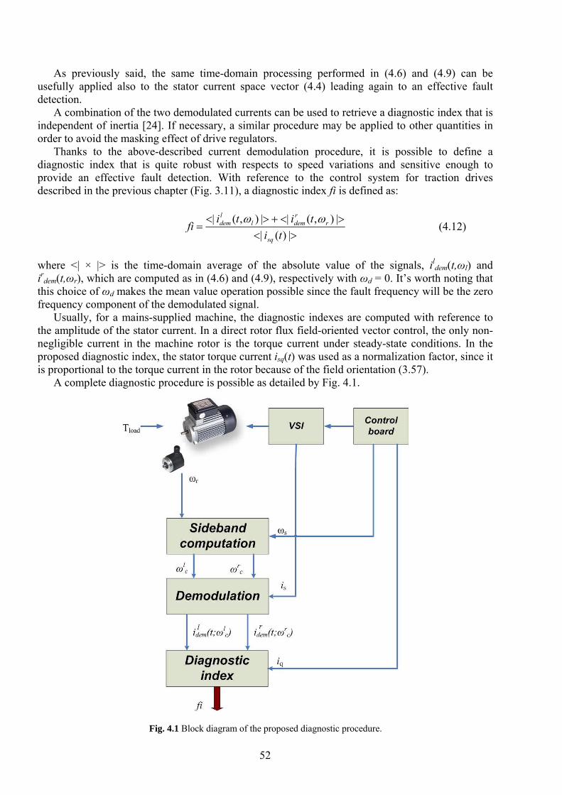
52
As previously said, the same time-domain processing performed in (4.6) and (4.9) can be usefully applied also to the stator current space vector (4.4) leading again to an effective fault detection.
A combination of the two demodulated currents can be used to retrieve a diagnostic index that is independent of inertia [24]. If necessary, a similar procedure may be applied to other quantities in order to avoid the masking effect of drive regulators.
Thanks to the above-described current demodulation procedure, it is possible to define a diagnostic index that is quite robust with respects to speed variations and sensitive enough to provide an effective fault detection. With reference to the control system for traction drives described in the previous chapter (Fig. 3.11), a diagnostic index fi is defined as:
><
><+><=
|)(||),(||),(|
tititifi
sq
rrdeml
ldem ωω
(4.12)
where <| × |> is the time-domain average of the absolute value of the signals, il
dem(t,ωl) and ir
dem(t,ωr), which are computed as in (4.6) and (4.9), respectively with ωd = 0. It’s worth noting that this choice of ωd makes the mean value operation possible since the fault frequency will be the zero frequency component of the demodulated signal.
Usually, for a mains-supplied machine, the diagnostic indexes are computed with reference to the amplitude of the stator current. In a direct rotor flux field-oriented vector control, the only non-negligible current in the machine rotor is the torque current under steady-state conditions. In the proposed diagnostic index, the stator torque current isq(t) was used as a normalization factor, since it is proportional to the torque current in the rotor because of the field orientation (3.57).
A complete diagnostic procedure is possible as detailed by Fig. 4.1.
Fig. 4.1 Block diagram of the proposed diagnostic procedure.
53
4.3. Virtual Current Technique
4.3.1. Introduction
This new technique has been developed with the aim to perform a quantification of the fault severity considering the influence of the closed loop control system. More specifically the Virtual Current Technique (VCT) is a model-based diagnostic technique, for the diagnosis of rotor faults in Direct Rotor Field Oriented Controlled (DRFOC) induction motor drives. By measuring the oscillations at twice the slip frequency found in the rotor flux of the machine, and by conjugating this information with the knowledge of some motor parameters, as well as the parameters of the flux and current controllers, it is possible to generate a virtual magnetizing current which, after normalization, allows the detection and quantification of the extension of the fault.
The proposed method allows to overcome the difficulties usually found in the diagnosis of rotor faults in closed loop drives, by providing information about the condition of the machine in a way independent of the bandwidth of the control loops. Although the VCT has been primarily developed for the traction drives used in railway applications described in the previous chapter, it could be incorporated in any DRFOC drive at almost no additional cost.
The diagnosis of rotor faults in line-fed induction motors has been a subject of research for the last three decades [2], [47], [64]-[68],. Nevertheless, nowadays an increasing number of motors is incorporated in closed-loop drives, whose control strategies, in most cases, rely on rotor field orientation. In these systems, the techniques developed for line-fed induction motors and open loop drives cannot be used straightforward as the control system of the drive changes the effects that the fault would introduce in several quantities, namely in the motor supply currents, and hence it does not allow a proper detection and quantification of the extension of the fault [51],[69-71]. Consequently, the need for development of adequate diagnostic techniques capable of diagnosing faults effectively in closed-loop drives is driving the research in this particular field of knowledge.
The ultimate goal is not only the detection and quantification of the faults but also the integration of the diagnostic and control systems of the drive on the same board, so that the manufacturer of the drive can provide to the customer a system with self-diagnostic capabilities [52],[61],[72], [73].
In [29],[74] we find one of the first papers proposing a model based method to diagnose rotor faults in vector-controlled induction motor drives, i.e. the Vienna Monitoring Method, whose fault indicator relies on the calculation of two values for the electromagnetic torque developed by the machine, one using a current model and the other one using a voltage model.
Anyway for closed loop drives the possibility of quantification of the extension of the fault and the role played by the tuning of the current, flux and speed controllers are still an open issue. In fact, as demonstrated in several papers [51], [69], [70], [75], [76], the topology of the control system as well as the choice of the parameters of the flux and speed controllers of the drive have a strong effect on the amplitudes of the fault indicators that may be defined to detect the fault.
In [51], it is presented a comprehensive analysis of the role played by the control system of the drive on the diagnosis of motor faults in closed-loop drives. The authors, recognizing the limitations of the classical diagnostic techniques, propose as an alternative to measure the oscillations present in the reference magnetizing current component i*
sd. They concluded that this fault indicator is quite independent of the control parameters, for the topology of the control system adopted (DRFOC) and for a fixed bandwidth of the flux control loop. In spite of these results, the authors do not provide a useful relationship between the oscillations present in i*
sd and the extension of the fault [70], [76]. On the other hand, the torque-producing current component i*
sq, due to its strong dependency with the operating conditions of the drive, is not adequate for diagnostic purposes as it depends heavily on the controller gains, load conditions and operating frequency of the drive.
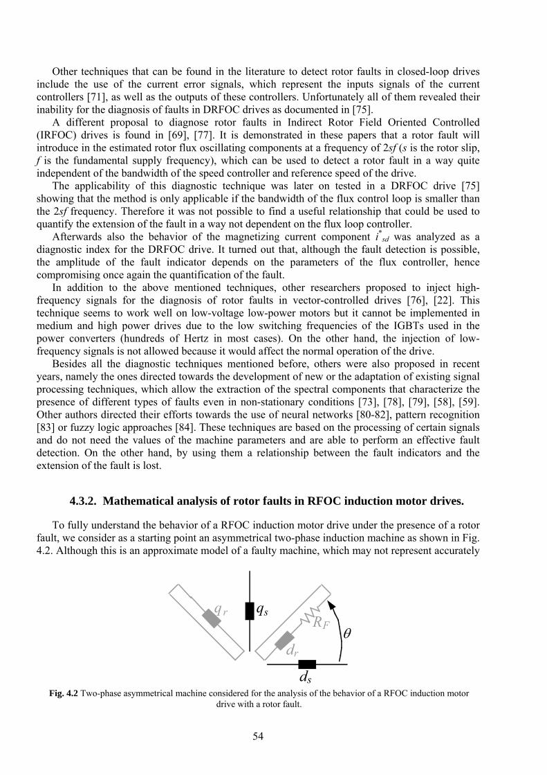
54
Other techniques that can be found in the literature to detect rotor faults in closed-loop drives include the use of the current error signals, which represent the inputs signals of the current controllers [71], as well as the outputs of these controllers. Unfortunately all of them revealed their inability for the diagnosis of faults in DRFOC drives as documented in [75].
A different proposal to diagnose rotor faults in Indirect Rotor Field Oriented Controlled (IRFOC) drives is found in [69], [77]. It is demonstrated in these papers that a rotor fault will introduce in the estimated rotor flux oscillating components at a frequency of 2sf (s is the rotor slip, f is the fundamental supply frequency), which can be used to detect a rotor fault in a way quite independent of the bandwidth of the speed controller and reference speed of the drive.
The applicability of this diagnostic technique was later on tested in a DRFOC drive [75] showing that the method is only applicable if the bandwidth of the flux control loop is smaller than the 2sf frequency. Therefore it was not possible to find a useful relationship that could be used to quantify the extension of the fault in a way not dependent on the flux loop controller.
Afterwards also the behavior of the magnetizing current component i*sd was analyzed as a
diagnostic index for the DRFOC drive. It turned out that, although the fault detection is possible, the amplitude of the fault indicator depends on the parameters of the flux controller, hence compromising once again the quantification of the fault.
In addition to the above mentioned techniques, other researchers proposed to inject high-frequency signals for the diagnosis of rotor faults in vector-controlled drives [76], [22]. This technique seems to work well on low-voltage low-power motors but it cannot be implemented in medium and high power drives due to the low switching frequencies of the IGBTs used in the power converters (hundreds of Hertz in most cases). On the other hand, the injection of low-frequency signals is not allowed because it would affect the normal operation of the drive.
Besides all the diagnostic techniques mentioned before, others were also proposed in recent years, namely the ones directed towards the development of new or the adaptation of existing signal processing techniques, which allow the extraction of the spectral components that characterize the presence of different types of faults even in non-stationary conditions [73], [78], [79], [58], [59]. Other authors directed their efforts towards the use of neural networks [80-82], pattern recognition [83] or fuzzy logic approaches [84]. These techniques are based on the processing of certain signals and do not need the values of the machine parameters and are able to perform an effective fault detection. On the other hand, by using them a relationship between the fault indicators and the extension of the fault is lost.
4.3.2. Mathematical analysis of rotor faults in RFOC induction motor drives.
To fully understand the behavior of a RFOC induction motor drive under the presence of a rotor fault, we consider as a starting point an asymmetrical two-phase induction machine as shown in Fig. 4.2. Although this is an approximate model of a faulty machine, which may not represent accurately
ds
dr
qr qsRF
rθ
Fig. 4.2 Two-phase asymmetrical machine considered for the analysis of the behavior of a RFOC induction motor
drive with a rotor fault.
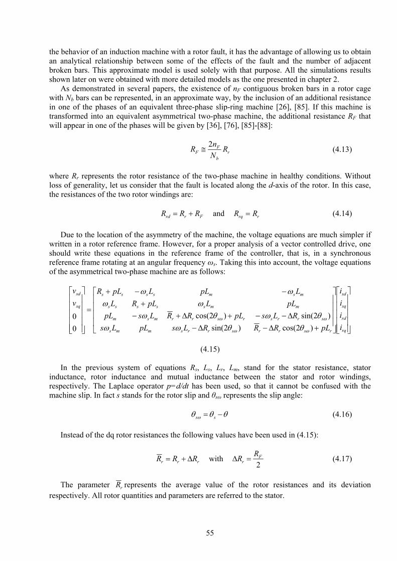
55
the behavior of an induction machine with a rotor fault, it has the advantage of allowing us to obtain an analytical relationship between some of the effects of the fault and the number of adjacent broken bars. This approximate model is used solely with that purpose. All the simulations results shown later on were obtained with more detailed models as the one presented in chapter 2.
As demonstrated in several papers, the existence of nF contiguous broken bars in a rotor cage with Nb bars can be represented, in an approximate way, by the inclusion of an additional resistance in one of the phases of an equivalent three-phase slip-ring machine [26], [85]. If this machine is transformed into an equivalent asymmetrical two-phase machine, the additional resistance RF that will appear in one of the phases will be given by [36], [76], [85]-[88]:
rb
FF R
NnR 2
≅ (4.13)
where Rr represents the rotor resistance of the two-phase machine in healthy conditions. Without loss of generality, let us consider that the fault is located along the d-axis of the rotor. In this case, the resistances of the two rotor windings are:
Frrd RRR += and rrq RR = (4.14) Due to the location of the asymmetry of the machine, the voltage equations are much simpler if
written in a rotor reference frame. However, for a proper analysis of a vector controlled drive, one should write these equations in the reference frame of the controller, that is, in a synchronous reference frame rotating at an angular frequency ωs. Taking this into account, the voltage equations of the asymmetrical two-phase machine are as follows:
⎥⎥⎥⎥⎥
⎦
⎤
⎢⎢⎢⎢⎢
⎣
⎡
⎥⎥⎥⎥
⎦
⎤
⎢⎢⎢⎢
⎣
⎡
+Δ−Δ−Δ−−+Δ+−
+−−+
=
⎥⎥⎥⎥⎥
⎦
⎤
⎢⎢⎢⎢⎢
⎣
⎡
rq
rd
sq
sd
rsrrsrrsmms
srrsrsrrmsm
mmsssss
msmssss
sq
sd
iiii
pLRRRLspLLsRLspLRRLspL
pLLpLRLLpLLpLR
vv
)2cos()2sin()2sin()2cos(
00
ωω
ωω
θθωωθωθω
ωωωω
(4.15) In the previous system of equations Rs, Ls, Lr, Lm, stand for the stator resistance, stator
inductance, rotor inductance and mutual inductance between the stator and rotor windings, respectively. The Laplace operator p=d/dt has been used, so that it cannot be confused with the machine slip. In fact s stands for the rotor slip and θsω represents the slip angle:
θθθ ω −= ss (4.16) Instead of the dq rotor resistances the following values have been used in (4.15):
rrr RRR Δ+= with 2
Fr
RR =Δ (4.17)
The parameter rR represents the average value of the rotor resistances and its deviation
respectively. All rotor quantities and parameters are referred to the stator.
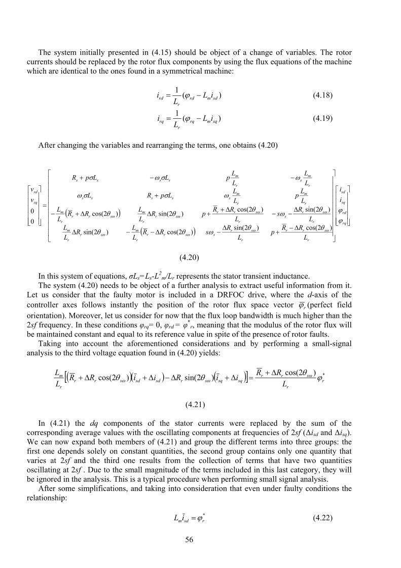
56
The system initially presented in (4.15) should be object of a change of variables. The rotor currents should be replaced by the rotor flux components by using the flux equations of the machine which are identical to the ones found in a symmetrical machine:
)(1sdmrd
rrd iL
Li −= ϕ (4.18)
)(1sqmrq
rrq iL
Li −= ϕ (4.19)
After changing the variables and rearranging the terms, one obtains (4.20)
( )
( )⎥⎥⎥⎥⎥
⎦
⎤
⎢⎢⎢⎢⎢
⎣
⎡
⎥⎥⎥⎥⎥⎥⎥⎥⎥
⎦
⎤
⎢⎢⎢⎢⎢⎢⎢⎢⎢
⎣
⎡
Δ−+
Δ−Δ−−Δ
Δ−−
Δ++ΔΔ+−
+
−−+
=
⎥⎥⎥⎥⎥
⎦
⎤
⎢⎢⎢⎢⎢
⎣
⎡
rq
rd
sq
sd
r
srr
r
srssrr
r
msr
r
m
r
srs
r
srrsr
r
msrr
r
m
r
m
r
msssss
r
ms
r
mssss
sq
sd
ii
LRRp
LRsRR
LLR
LL
LRs
LRRpR
LLRR
LL
LLp
LLLpRL
LL
LLpLLpR
vv
ϕϕ
θθωθθ
θωθθθ
ωσσω
ωσωσ
ωωωω
ωωωω
)2cos()2sin()2cos()2sin(
)2sin()2cos()2sin()2cos(00
(4.20) In this system of equations, σLs=Ls-L2
m/Lr represents the stator transient inductance. The system (4.20) needs to be object of a further analysis to extract useful information from it.
Let us consider that the faulty motor is included in a DRFOC drive, where the d-axis of the controller axes follows instantly the position of the rotor flux space vector rϕ (perfect field orientation). Moreover, let us consider for now that the flux loop bandwidth is much higher than the 2sf frequency. In these conditions φrq= 0, φrd = φ*
r, meaning that the modulus of the rotor flux will be maintained constant and equal to its reference value in spite of the presence of rotor faults.
Taking into account the aforementioned considerations and by performing a small-signal analysis to the third voltage equation found in (4.20) yields:
( )( ) ( )[ ] *)2cos()2sin()2cos( rr
srrsqsqsrsdsdsrr
r
m
LRRiiRiiRR
LL ϕθθθ ω
ωωΔ+
=Δ+Δ−Δ+Δ+
(4.21)
In (4.21) the dq components of the stator currents were replaced by the sum of the
corresponding average values with the oscillating components at frequencies of 2sf (Δisd and Δisq). We can now expand both members of (4.21) and group the different terms into three groups: the first one depends solely on constant quantities, the second group contains only one quantity that varies at 2sf and the third one results from the collection of terms that have two quantities oscillating at 2sf . Due to the small magnitude of the terms included in this last category, they will be ignored in the analysis. This is a typical procedure when performing small signal analysis.
After some simplifications, and taking into consideration that even under faulty conditions the relationship:
*
rsdmiL ϕ= (4.22)
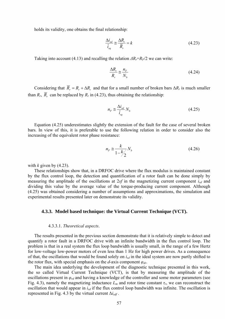
57
holds its validity, one obtains the final relationship:
kRR
ii
r
r
sq
sd =Δ
≅Δ (4.23)
Taking into account (4.13) and recalling the relation ΔRr=RF/2 we can write:
b
F
r
r
Nn
RR
≅Δ (4.24)
Considering that rrr RRR Δ+= and that for a small number of broken bars ΔRr is much smaller
than Rr, rR can be replaced by Rr in (4.23), thus obtaining the relationship:
bsq
sdF N
iin Δ
≅ (4.25)
Equation (4.25) underestimates slightly the extension of the fault for the case of several broken
bars. In view of this, it is preferable to use the following relation in order to consider also the increasing of the equivalent rotor phase resistance:
bF Nkkn
21−≅ (4.26)
with k given by (4.23).
These relationships show that, in a DRFOC drive where the flux modulus is maintained constant by the flux control loop, the detection and quantification of a rotor fault can be done simply by measuring the amplitude of the oscillations at 2sf in the magnetizing current component isd and dividing this value by the average value of the torque-producing current component. Although (4.25) was obtained considering a number of assumptions and approximations, the simulation and experimental results presented later on demonstrate its validity.
4.3.3. Model based technique: the Virtual Current Technique (VCT).
4.3.3.1. Theoretical aspects.
The results presented in the previous section demonstrate that it is relatively simple to detect and quantify a rotor fault in a DRFOC drive with an infinite bandwidth in the flux control loop. The problem is that in a real system the flux loop bandwidth is usually small, in the range of a few Hertz for low-voltage low-power motors of even less than 1 Hz for high power drives. As a consequence of that, the oscillations that would be found solely on isd in the ideal system are now partly shifted to the rotor flux, with special emphasis on the d-axis component φdr.
The main idea underlying the development of the diagnostic technique presented in this work, the so called Virtual Current Technique (VCT), is that by measuring the amplitude of the oscillations present in φrd and having a knowledge of the controller and some motor parameters (see Fig. 4.3), namely the magnetizing inductance Lm and rotor time constant τr, we can reconstruct the oscillation that would appear in isd if the flux control loop bandwidth was infinite. The oscillation is represented in Fig. 4.3 by the virtual current Δisdf .
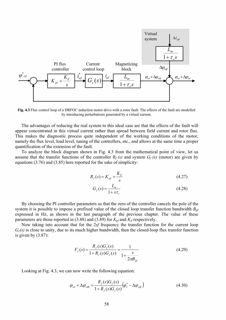
58
The advantages of reducing the real system to this ideal case are that the effects of the fault will appear concentrated in this virtual current rather than spread between field current and rotor flux. This makes the diagnostic process quite independent of the working conditions of the motor, namely the flux level, load level, tuning of the controllers, etc., and allows at the same time a proper quantification of the extension of the fault.
To analyze the block diagram shown in Fig. 4.3 from the mathematical point of view, let us assume that the transfer functions of the controller Rf (s) and system Gf (s) (motor) are given by equations (3.76) and (3.85) here reported for the sake of simplicity:
s
KKsR if
pff +=)( (4.27)
r
mf s
LsGτ+
=1
)( (4.28)
By choosing the PI controller parameters so that the zero of the controller cancels the pole of the
system it is possible to impose a prefixed value of the closed loop transfer function bandwidth Bpf expressed in Hz, as shown in the last paragraph of the previous chapter. The value of these parameters are those reported in (3.88) and (3.89) for Kpf and Kif respectively.
Now taking into account that for the 2sf frequency the transfer function for the current loop Gc(s) is close to unity, due to its much higher bandwidth, then the closed-loop flux transfer function is given by (3.87):
pf
ff
fff
BssGsR
sGsRsF
π21
1)()(1
)()()(
+=
+= (4.29)
Looking at Fig. 4.3, we can now write the following equation:
( )rdfrff
ffrdhrd sGsR
sGsRϕϕϕϕ Δ−
+=Δ+ *
)()(1)()(
(4.30)
PI flux controller
Current control loop
Magnetizingblock
Virtualsystem
sL
r
m
τ+1
sL
r
m
τ+1
)(sGcsK
K ifpf +
sdfiΔ
sdi*sdird
*ϕrdhrd ϕϕ Δ+ rdrd ϕϕ Δ+
rdfϕΔ
Fig. 4.3 Flux control loop of a DRFOC induction motor drive with a rotor fault. The effects of the fault are modelled by introducing perturbations generated by a virtual current.
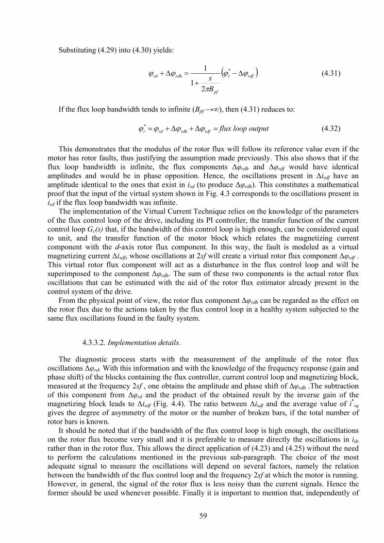
59
Substituting (4.29) into (4.30) yields:
( )rdfr
pf
rdhrd
Bs ϕϕ
π
ϕϕ Δ−+
=Δ+ *
21
1 (4.31)
If the flux loop bandwidth tends to infinite (Bpf →∞), then (4.31) reduces to: =Δ+Δ+= rdfrdhrdr ϕϕϕϕ* flux loop output (4.32) This demonstrates that the modulus of the rotor flux will follow its reference value even if the
motor has rotor faults, thus justifying the assumption made previously. This also shows that if the flux loop bandwidth is infinite, the flux components Δφrdh and Δφrdf would have identical amplitudes and would be in phase opposition. Hence, the oscillations present in Δisdf have an amplitude identical to the ones that exist in isd (to produce Δφrdh). This constitutes a mathematical proof that the input of the virtual system shown in Fig. 4.3 corresponds to the oscillations present in isd if the flux loop bandwidth was infinite.
The implementation of the Virtual Current Technique relies on the knowledge of the parameters of the flux control loop of the drive, including its PI controller, the transfer function of the current control loop Gc(s) that, if the bandwidth of this control loop is high enough, can be considered equal to unit, and the transfer function of the motor block which relates the magnetizing current component with the d-axis rotor flux component. In this way, the fault is modeled as a virtual magnetizing current Δisdf, whose oscillations at 2sf will create a virtual rotor flux component Δφrdf . This virtual rotor flux component will act as a disturbance in the flux control loop and will be superimposed to the component Δφrdh. The sum of these two components is the actual rotor flux oscillations that can be estimated with the aid of the rotor flux estimator already present in the control system of the drive.
From the physical point of view, the rotor flux component Δφrdh can be regarded as the effect on the rotor flux due to the actions taken by the flux control loop in a healthy system subjected to the same flux oscillations found in the faulty system.
4.3.3.2. Implementation details.
The diagnostic process starts with the measurement of the amplitude of the rotor flux oscillations Δφrd. With this information and with the knowledge of the frequency response (gain and phase shift) of the blocks containing the flux controller, current control loop and magnetizing block, measured at the frequency 2sf , one obtains the amplitude and phase shift of Δφrdh .The subtraction of this component from Δφrd and the product of the obtained result by the inverse gain of the magnetizing block leads to Δisdf (Fig. 4.4). The ratio between Δisdf and the average value of i*
sq gives the degree of asymmetry of the motor or the number of broken bars, if the total number of rotor bars is known.
It should be noted that if the bandwidth of the flux control loop is high enough, the oscillations on the rotor flux become very small and it is preferable to measure directly the oscillations in ids rather than in the rotor flux. This allows the direct application of (4.23) and (4.25) without the need to perform the calculations mentioned in the previous sub-paragraph. The choice of the most adequate signal to measure the oscillations will depend on several factors, namely the relation between the bandwidth of the flux control loop and the frequency 2sf at which the motor is running. However, in general, the signal of the rotor flux is less noisy than the current signals. Hence the former should be used whenever possible. Finally it is important to mention that, independently of
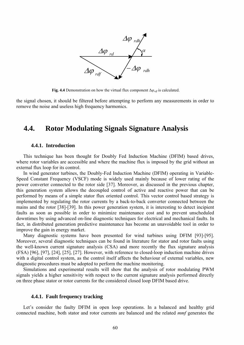
60
the signal chosen, it should be filtered before attempting to perform any measurements in order to remove the noise and useless high frequency harmonics.
4.4. Rotor Modulating Signals Signature Analysis
4.4.1. Introduction
This technique has been thought for Doubly Fed Induction Machine (DFIM) based drives, where rotor variables are accessible and where the machine flux is imposed by the grid without an external flux loop for its control.
In wind generator turbines, the Doubly-Fed Induction Machine (DFIM) operating in Variable-Speed Constant Frequency (VSCF) mode is widely used mainly because of lower rating of the power converter connected to the rotor side [37]. Moreover, as discussed in the previous chapter, this generation system allows the decoupled control of active and reactive power that can be performed by means of a simple stator flux oriented control. This vector control based strategy is implemented by regulating the rotor currents by a back-to-back converter connected between the mains and the rotor [38]-[39]. In this power generation system, it is interesting to detect incipient faults as soon as possible in order to minimize maintenance cost and to prevent unscheduled downtimes by using advanced on-line diagnostic techniques for electrical and mechanical faults. In fact, in distributed generation predictive maintenance has become an unavoidable tool in order to improve the gain in energy market.
Many diagnostic systems have been presented for wind turbines using DFIM [93]-[95]. Moreover, several diagnostic techniques can be found in literature for stator and rotor faults using the well-known current signature analysis (CSA) and more recently the flux signature analysis (FSA) [96], [97], [24], [25], [27]. However, with reference to closed-loop induction machine drives with a digital control system, as the control itself affects the behaviour of external variables, new diagnostic procedures must be adopted to perform the machine monitoring.
Simulations and experimental results will show that the analysis of rotor modulating PWM signals yields a higher sensitivity with respect to the current signature analysis performed directly on three phase stator or rotor currents for the considered closed loop DFIM based drive.
4.4.1. Fault frequency tracking
Let’s consider the faulty DFIM in open loop operations. In a balanced and healthy grid connected machine, both stator and rotor currents are balanced and the related mmf generates the
rdΔϕrdhΔϕ
rdh−ΔϕrdfΔϕ
α
Fig. 4.4 Demonstration on how the virtual flux component Δφrdf is calculated.
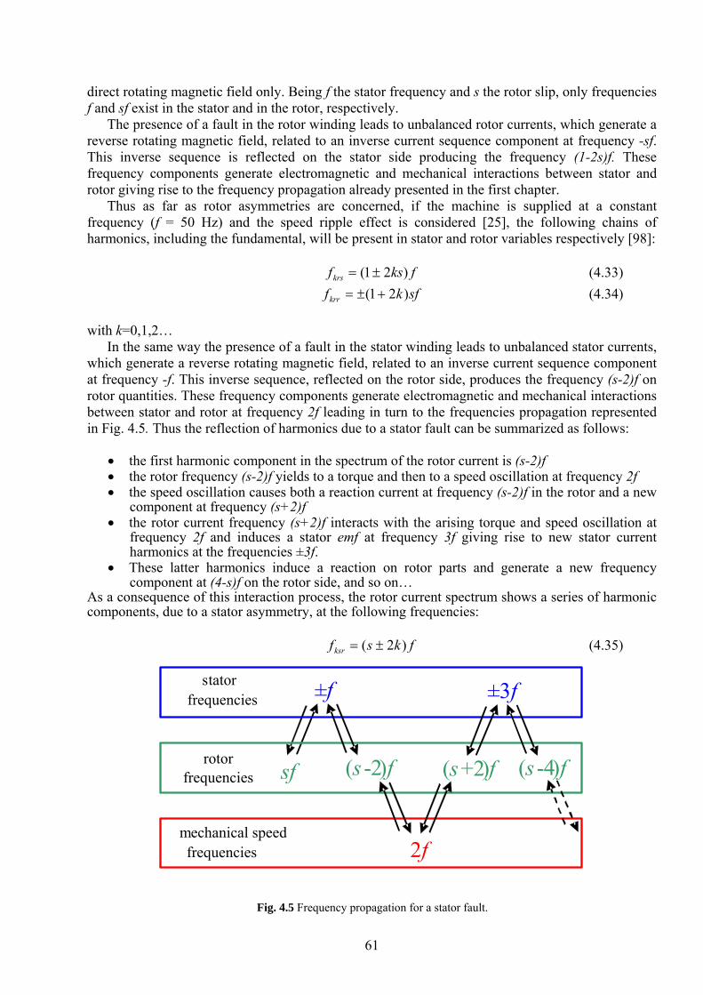
61
direct rotating magnetic field only. Being f the stator frequency and s the rotor slip, only frequencies f and sf exist in the stator and in the rotor, respectively.
The presence of a fault in the rotor winding leads to unbalanced rotor currents, which generate a reverse rotating magnetic field, related to an inverse current sequence component at frequency -sf. This inverse sequence is reflected on the stator side producing the frequency (1-2s)f. These frequency components generate electromagnetic and mechanical interactions between stator and rotor giving rise to the frequency propagation already presented in the first chapter.
Thus as far as rotor asymmetries are concerned, if the machine is supplied at a constant frequency (f = 50 Hz) and the speed ripple effect is considered [25], the following chains of harmonics, including the fundamental, will be present in stator and rotor variables respectively [98]:
fksfkrs )21( ±= (4.33) sfkfkrr )21( +±= (4.34)
with k=0,1,2… In the same way the presence of a fault in the stator winding leads to unbalanced stator currents,
which generate a reverse rotating magnetic field, related to an inverse current sequence component at frequency -f. This inverse sequence, reflected on the rotor side, produces the frequency (s-2)f on rotor quantities. These frequency components generate electromagnetic and mechanical interactions between stator and rotor at frequency 2f leading in turn to the frequencies propagation represented in Fig. 4.5. Thus the reflection of harmonics due to a stator fault can be summarized as follows:
• the first harmonic component in the spectrum of the rotor current is (s-2)f • the rotor frequency (s-2)f yields to a torque and then to a speed oscillation at frequency 2f • the speed oscillation causes both a reaction current at frequency (s-2)f in the rotor and a new
component at frequency (s+2)f • the rotor current frequency (s+2)f interacts with the arising torque and speed oscillation at
frequency 2f and induces a stator emf at frequency 3f giving rise to new stator current harmonics at the frequencies ±3f.
• These latter harmonics induce a reaction on rotor parts and generate a new frequency component at (4-s)f on the rotor side, and so on…
As a consequence of this interaction process, the rotor current spectrum shows a series of harmonic components, due to a stator asymmetry, at the following frequencies:
fksfksr )2( ±= (4.35)
rotor frequencies sf (s -2)f
±f ±3f
2f mechanical speed frequencies
stator frequencies
(s+2)f (s -4)f
Fig. 4.5 Frequency propagation for a stator fault.
62
whereas stator currents will present the following chain of frequencies: fkfkss )21( +±= (4.36)
with k=0,1,2… This discussion shows that a rotor or a stator dissymmetry is directly reflected on the current
spectra of both stator and rotor currents. The diagnosis method using current signature analysis are based on monitoring particular stator
or rotor current frequencies related to stator or rotor faults. In particular, for a rotor fault, the most relevant frequencies are (1-2s)f in the stator currents and -sf in the rotor currents (i.e. the first order fault harmonics coming from (4.33) and (4.34) respectively). In the case of stator fault the most relevant frequencies are -f in the stator currents and (s-2)f in the rotor currents (i.e. the first order fault harmonics coming from (4.36) and (4.35) respectively).
As far as closed loop operations are concerned, the rotor current control loops will try to follow sinusoidal and balanced current references by applying unbalanced rotor voltages. Consequently, the typical rotor and stator current fault harmonic components might become less visible due to the compensating action of the control system. On the contrary, these fault harmonic components remain clearly observable in the rotor modulating signals, allowing the rotor modulating signals to be considered as new effective diagnostic index for the detection of stator an rotor asymmetries in DFIMs.
Therefore according to (4.35) a stator fault is expected to produce a relevant harmonic in the rotor modulating signals space vector at the frequency:
fsfsrv )2( −= (4.37) This frequency corresponds to a positive harmonic component at frequency (2-s)f for each rotor
modulating signal, where f is the stator voltage frequency coming from the grid. On the other hand according to (4.34) a rotor fault is expected to produce a negative sequence
harmonic component in the spectrum of the rotor modulating signals at the frequency: sffrrv −= (4.38) The presence of an inverse sequence component in the rotor modulating signals can be detected
by applying the FFT to their space vector representation.
4.4.2. Closed loop bandwidth impact
As proven in the previous paragraph with reference to squirrel cage induction motors, currents signature keeps its sensitivity to rotor faults only if the bandwidth of the external flux loop is high enough in respect to the fault frequencies. Here reference is made to a drive in which the flux is imposed by the grid connected to the stator and where rotor currents are imposed by two internal current loops. Thus if closed loop operations of the drive are considered, the rotor current regulators will try to impose sinusoidal and balanced currents in the rotor windings even in case of faulty machine. As a consequence if the motor is not symmetric, the control system generates unbalanced rotor voltages and so unbalanced rotor modulating PWM signals in order to balance the currents. These signals will contain new fault spectral components which can be easily detected by frequency analysis. This frequency analysis can be considered as an improvement of the diagnostic techniques already developed for squirrel-cage three-phase induction machine directly connected to the grid [94], [24], [25], [27].
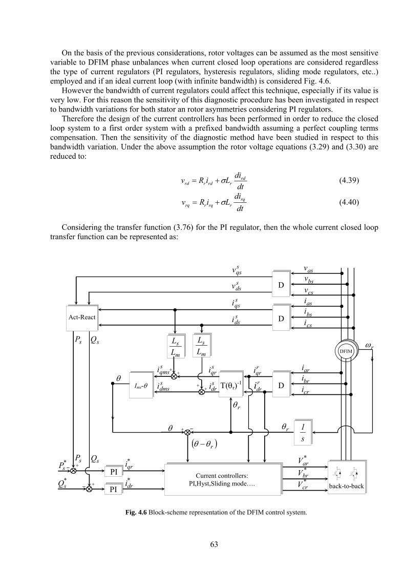
63
On the basis of the previous considerations, rotor voltages can be assumed as the most sensitive variable to DFIM phase unbalances when current closed loop operations are considered regardless the type of current regulators (PI regulators, hysteresis regulators, sliding mode regulators, etc..) employed and if an ideal current loop (with infinite bandwidth) is considered Fig. 4.6.
However the bandwidth of current regulators could affect this technique, especially if its value is very low. For this reason the sensitivity of this diagnostic procedure has been investigated in respect to bandwidth variations for both stator an rotor asymmetries considering PI regulators.
Therefore the design of the current controllers has been performed in order to reduce the closed loop system to a first order system with a prefixed bandwidth assuming a perfect coupling terms compensation. Then the sensitivity of the diagnostic method have been studied in respect to this bandwidth variation. Under the above assumption the rotor voltage equations (3.29) and (3.30) are reduced to:
dt
diLiRv rdrrdrrd σ+= (4.39)
dt
diLiRv rq
rrqrrq σ+= (4.40)
Considering the transfer function (3.76) for the PI regulator, then the whole current closed loop
transfer function can be represented as:
DFIM
back-to-back
D
T(θr)-1Ims-θ
PI
PI
Act-React
asibsi
csi
s1
rω
rqrirdri
sqsisdsi
sqrisdri
m
sLL
sqmsisdmsi
θ
rθ
( )rθθ −
*qri
*dri
*sP
*sQ
θ
sP sQ
sP sQ+
+
+
++
++
rθ
D
sqsvsdsv
asvbsv
csv
m
sLL
D
aribri
cri
Current controllers: PI,Hyst,Sliding mode….
*arV*brV*crV
Fig. 4.6 Block-scheme representation of the DFIM control system.

64
pi
rc
BssG
π21
1)(+
= (4.41)
where Bpi is the closed loop bandwidth and the proportional and integral gains of the controller are:
rpipc LBK σπ2= (4.42) rpiic RBK π2= (4.43) In case of unbalanced stator or rotor windings the rotor current loops try to follow sinusoidal
and balanced currents references by applying unbalanced rotor voltages in a way dependent on (4.42) and (4.43). So the typical fault frequencies usually present in the currents, due to stator and rotor asymmetries will be damped by the action of the control system and they will be transferred to rotor voltages in a way dependent on the closed loop bandwidth Bpi.
65
Chapter 5
Simulation Results
5.1. Introduction
All the control schemes described in Chapter 3 has been implemented in Matlab Simulink®. The choice of this environment was made due to its simplicity and because the power converters and more in general the whole power system, used in the experimental setup is controlled by a dSpace® DS 1103 board which is fully programmable from the Simulink® block diagram environment. Part of the control schemes used for the simulations can be reused in the dSPACE environment by the C-code production generator (RTW), to be compiled and downloaded to dSPACE board.
Moreover Simulink offers an embedded set of tools (SimPowerSystems) for the simulation of electrical systems. Unfortunately, although they are enough accurate for the simulation of the converter circuits, they do not provide sufficiently detailed electrical machine models, for our investigation.
To overcome this limitation the S-Function block of Simulink was employed. This block was born specifically to implement continuous and discrete systems in the input-state-output form. Hence, Matlab user can employ S-Functions to describe systems which are not present in Simulink library writing them in M-code. The simplicity of M-code and S-Function structure allows the user to make up the simulation easily and quickly.
In our case the S-function block has been used to implement the set of differential equations deriving from the developed machine models in order to exploit the MATLAB® variable step ODE (Ordinary Differential Equations) solvers. This set of differential equations has to be expressed in the input-state-output form as shown in chapter 2.
Finally to realize simulations as close as possible to the real system, Simulink offers the opportunity to simulate hybrid systems, i.e. continuous time systems (the machine) and discrete time systems (the digital control). This can be done by employing specific triggered or function call blocks, whose execution is performed at fixed and discrete time steps and can be eventually managed by a state machine of higher level.
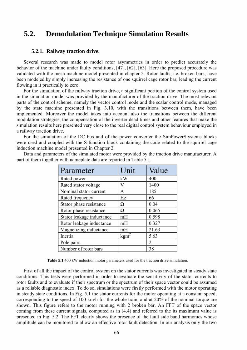
66
5.2. Demodulation Technique Simulation Results
5.2.1. Railway traction drive.
Several research was made to model rotor asymmetries in order to predict accurately the behavior of the machine under faulty conditions, [47], [62], [63]. Here the proposed procedure was validated with the mesh machine model presented in chapter 2. Rotor faults, i.e. broken bars, have been modeled by simply increasing the resistance of one squirrel cage rotor bar, leading the current flowing in it practically to zero.
For the simulation of the railway traction drive, a significant portion of the control system used in the simulation model was provided by the manufacturer of the traction drive. The most relevant parts of the control scheme, namely the vector control mode and the scalar control mode, managed by the state machine presented in Fig. 3.10, with the transitions between them, have been implemented. Moreover the model takes into account also the transitions between the different modulation strategies, the compensation of the inverter dead times and other features that make the simulation results here presented very close to the real digital control system behaviour employed in a railway traction drive.
For the simulation of the DC bus and of the power converter the SimPowerStystems blocks were used and coupled with the S-function block containing the code related to the squirrel cage induction machine model presented in Chapter 2.
Data and parameters of the simulated motor were provided by the traction drive manufacturer. A part of them together with nameplate data are reported in Table 5.1.
First of all the impact of the control system on the stator currents was investigated in steady state conditions. This tests were performed in order to evaluate the sensitivity of the stator currents to rotor faults and to evaluate if their spectrum or the spectrum of their space vector could be assumed as a reliable diagnostic index. To do so, simulations were firstly performed with the motor operating in steady state conditions. In Fig. 5.1 the stator currents for the motor operating at a constant speed, corresponding to the speed of 100 km/h for the whole train, and at 20% of the nominal torque are shown. This figure refers to the motor running with 2 broken bar. An FFT of the space vector coming from these current signals, computed as in (4.4) and referred to the its maximum value is presented in Fig. 5.2. The FFT clearly shows the presence of the fault side band harmonics whose amplitude can be monitored to allow an effective rotor fault detection. In our analysis only the two
Parameter Unit Value Rated power kW 400 Rated stator voltage V 1400 Nominal stator current A 185 Rated frequency Hz 66 Stator phase resistance Ω 0.04 Rotor phase resistance Ω 0.065 Stator leakage inductance mH 0.598 Rotor leakage inductance mH 0.327 Magnetizing inductance mH 21.63 Inertia kgm2 5.63 Pole pairs 2 Number of rotor bars 38
Table 5.1 400 kW induction motor parameters used for the traction drive simulation.
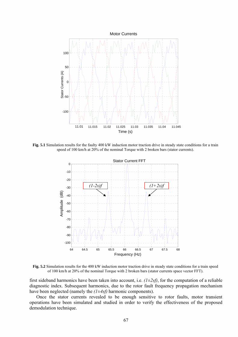
67
first sideband harmonics have been taken into account, i.e. (1±2sf), for the computation of a reliable diagnostic index. Subsequent harmonics, due to the rotor fault frequency propagation mechanism have been neglected (namely the (1±4sf) harmonic components).
Once the stator currents revealed to be enough sensitive to rotor faults, motor transient operations have been simulated and studied in order to verify the effectiveness of the proposed demodulation technique.
11.01 11.015 11.02 11.025 11.03 11.035 11.04 11.045
-100
-50
0
50
100
Time (s)
Sta
tor C
urre
nts
(A)
Motor Currents
Fig. 5.1 Simulation results for the faulty 400 kW induction motor traction drive in steady state conditions for a train
speed of 100 km/h at 20% of the nominal Torque with 2 broken bars (stator currents).
64 64.5 65 65.5 66 66.5 67 67.5 68
-100
-90
-80
-70
-60
-50
-40
-30
-20
-10
0Stator Current FFT
Ampl
itude
(dB
)
Frequency (Hz)
Fig. 5.2 Simulation results for the 400 kW induction motor traction drive in steady state conditions for a train speed of 100 km/h at 20% of the nominal Torque with 2 broken bars (stator currents space vector FFT).
(1-2s)f (1+2s)f
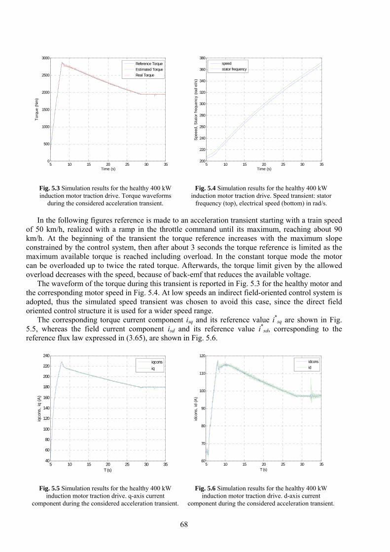
68
In the following figures reference is made to an acceleration transient starting with a train speed of 50 km/h, realized with a ramp in the throttle command until its maximum, reaching about 90 km/h. At the beginning of the transient the torque reference increases with the maximum slope constrained by the control system, then after about 3 seconds the torque reference is limited as the maximum available torque is reached including overload. In the constant torque mode the motor can be overloaded up to twice the rated torque. Afterwards, the torque limit given by the allowed overload decreases with the speed, because of back-emf that reduces the available voltage.
The waveform of the torque during this transient is reported in Fig. 5.3 for the healthy motor and the corresponding motor speed in Fig. 5.4. At low speeds an indirect field-oriented control system is adopted, thus the simulated speed transient was chosen to avoid this case, since the direct field oriented control structure it is used for a wider speed range.
The corresponding torque current component isq and its reference value i*sq are shown in Fig.
5.5, whereas the field current component isd and its reference value i*sd, corresponding to the
reference flux law expressed in (3.65), are shown in Fig. 5.6.
5 10 15 20 25 30 350
500
1000
1500
2000
2500
3000PLU 04-Jun-2007
T (s)
Tref
,Cou
rel,T
orf,(
Nm
)
Reference TorqueEstimated TorqueReal Torque
5 10 15 20 25 30 35200
220
240
260
280
300
320
340
360
380
T(s)
Spe
eed,
Sta
tor f
requ
ency
(rad
el/s
)
speedstator frequency
Fig. 5.3 Simulation results for the healthy 400 kW induction motor traction drive. Torque waveforms
during the considered acceleration transient.
Fig. 5.4 Simulation results for the healthy 400 kW
induction motor traction drive. Speed transient: stator frequency (top), electrical speed (bottom) in rad/s.
Time (s)
Torq
ue (N
m)
Time (s)
5 10 15 20 25 30 3540
60
80
100
120
140
160
180
200
220
240PLU 04-Jun-2007
T (s)
iqco
ns, i
q (A
)
iqconsiq
5 10 15 20 25 30 3560
70
80
90
100
110
120PLU 04-Jun-2007
T (s)
idco
ns, i
d (A
)
idconsid
Fig. 5.5 Simulation results for the healthy 400 kW
induction motor traction drive. q-axis current component during the considered acceleration transient.
Fig. 5.6 Simulation results for the healthy 400 kW
induction motor traction drive. d-axis current component during the considered acceleration transient.
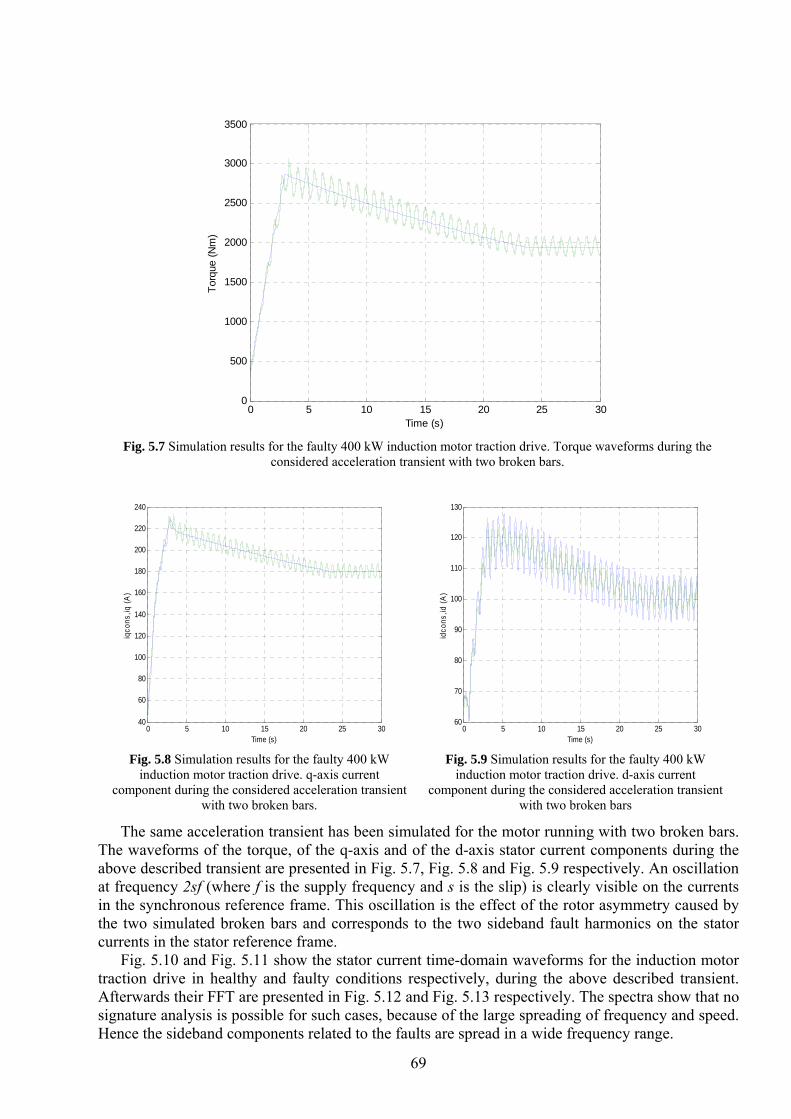
69
The same acceleration transient has been simulated for the motor running with two broken bars. The waveforms of the torque, of the q-axis and of the d-axis stator current components during the above described transient are presented in Fig. 5.7, Fig. 5.8 and Fig. 5.9 respectively. An oscillation at frequency 2sf (where f is the supply frequency and s is the slip) is clearly visible on the currents in the synchronous reference frame. This oscillation is the effect of the rotor asymmetry caused by the two simulated broken bars and corresponds to the two sideband fault harmonics on the stator currents in the stator reference frame.
Fig. 5.10 and Fig. 5.11 show the stator current time-domain waveforms for the induction motor traction drive in healthy and faulty conditions respectively, during the above described transient. Afterwards their FFT are presented in Fig. 5.12 and Fig. 5.13 respectively. The spectra show that no signature analysis is possible for such cases, because of the large spreading of frequency and speed. Hence the sideband components related to the faults are spread in a wide frequency range.
0 5 10 15 20 25 300
500
1000
1500
2000
2500
3000
3500
Time (s)
Torq
ue (N
m)
Fig. 5.7 Simulation results for the faulty 400 kW induction motor traction drive. Torque waveforms during the
considered acceleration transient with two broken bars.
0 5 10 15 20 25 3040
60
80
100
120
140
160
180
200
220
240
Time (s)
iqco
ns,iq
(A)
0 5 10 15 20 25 3060
70
80
90
100
110
120
130
Time (s)
idco
ns,id
(A)
Fig. 5.8 Simulation results for the faulty 400 kW induction motor traction drive. q-axis current
component during the considered acceleration transient with two broken bars.
Fig. 5.9 Simulation results for the faulty 400 kW induction motor traction drive. d-axis current
component during the considered acceleration transient with two broken bars
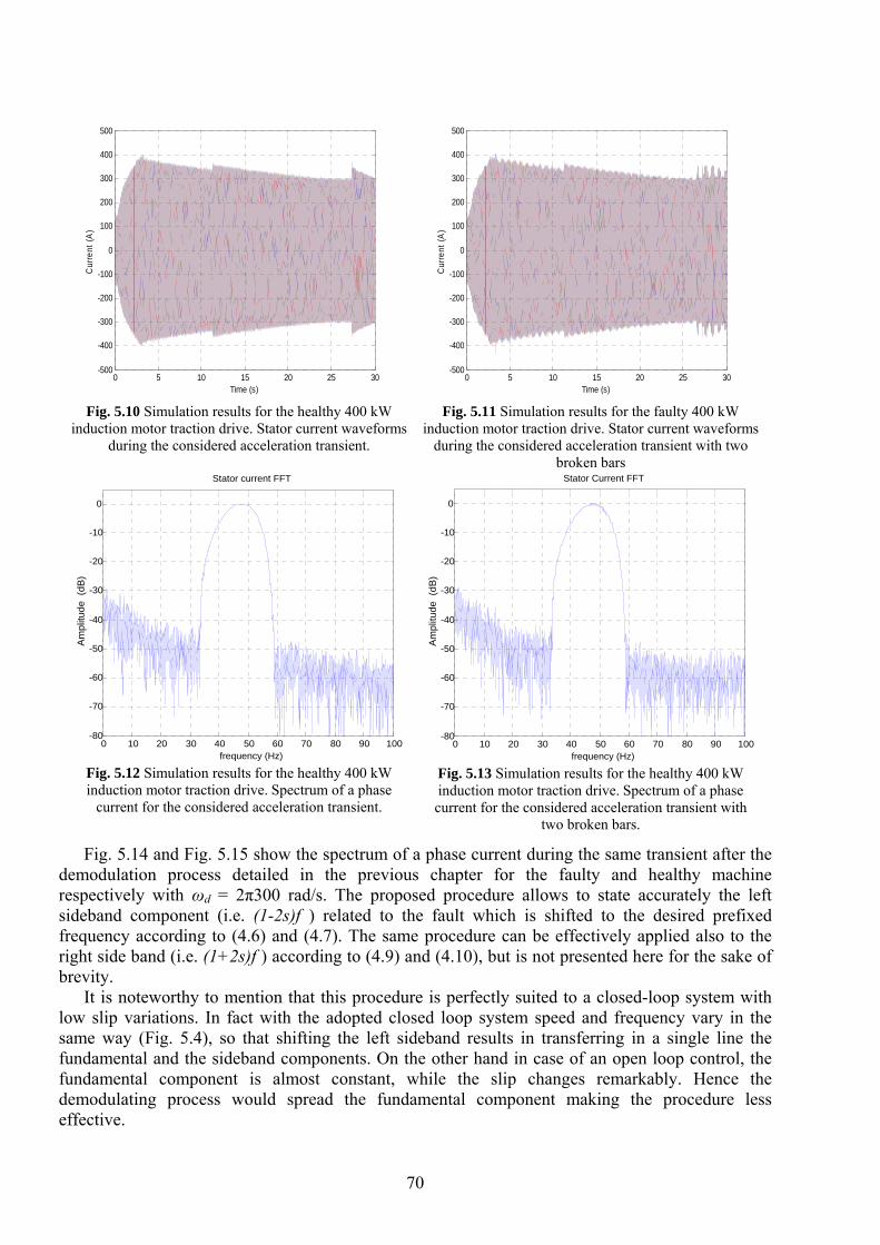
70
Fig. 5.14 and Fig. 5.15 show the spectrum of a phase current during the same transient after the demodulation process detailed in the previous chapter for the faulty and healthy machine respectively with ωd = 2π300 rad/s. The proposed procedure allows to state accurately the left sideband component (i.e. (1-2s)f ) related to the fault which is shifted to the desired prefixed frequency according to (4.6) and (4.7). The same procedure can be effectively applied also to the right side band (i.e. (1+2s)f ) according to (4.9) and (4.10), but is not presented here for the sake of brevity.
It is noteworthy to mention that this procedure is perfectly suited to a closed-loop system with low slip variations. In fact with the adopted closed loop system speed and frequency vary in the same way (Fig. 5.4), so that shifting the left sideband results in transferring in a single line the fundamental and the sideband components. On the other hand in case of an open loop control, the fundamental component is almost constant, while the slip changes remarkably. Hence the demodulating process would spread the fundamental component making the procedure less effective.
0 5 10 15 20 25 30-500
-400
-300
-200
-100
0
100
200
300
400
500
Time (s)
Cur
rent
(A)
Fig. 5.10 Simulation results for the healthy 400 kW induction motor traction drive. Stator current waveforms
during the considered acceleration transient.
0 5 10 15 20 25 30-500
-400
-300
-200
-100
0
100
200
300
400
500
Time (s)
Cur
rent
(A)
Fig. 5.11 Simulation results for the faulty 400 kW
induction motor traction drive. Stator current waveforms during the considered acceleration transient with two
broken bars
0 10 20 30 40 50 60 70 80 90 100-80
-70
-60
-50
-40
-30
-20
-10
0
Stator current FFT
Am
plitu
de (
dB)
frequency (Hz) Fig. 5.12 Simulation results for the healthy 400 kW induction motor traction drive. Spectrum of a phase
current for the considered acceleration transient.
0 10 20 30 40 50 60 70 80 90 100-80
-70
-60
-50
-40
-30
-20
-10
0
Stator Current FFT
Am
plitu
de (
dB)
frequency (Hz) Fig. 5.13 Simulation results for the healthy 400 kW induction motor traction drive. Spectrum of a phase current for the considered acceleration transient with
two broken bars.
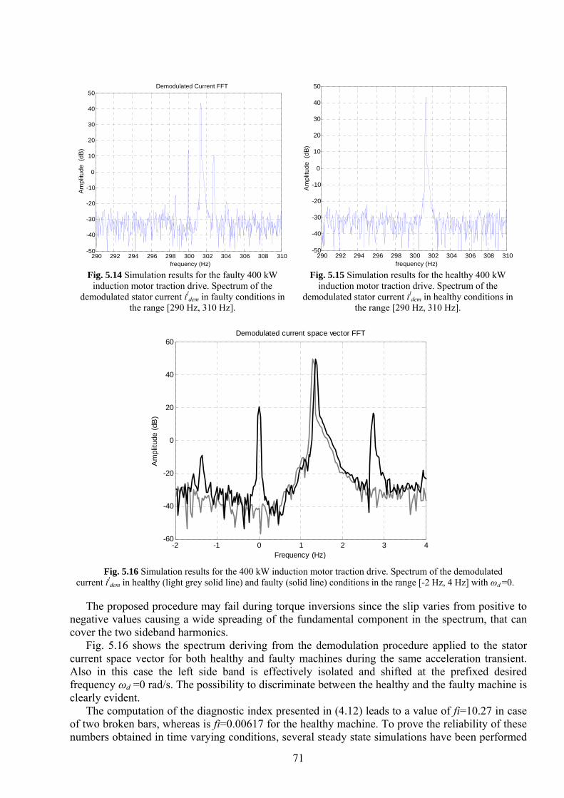
71
The proposed procedure may fail during torque inversions since the slip varies from positive to negative values causing a wide spreading of the fundamental component in the spectrum, that can cover the two sideband harmonics.
Fig. 5.16 shows the spectrum deriving from the demodulation procedure applied to the stator current space vector for both healthy and faulty machines during the same acceleration transient. Also in this case the left side band is effectively isolated and shifted at the prefixed desired frequency ωd =0 rad/s. The possibility to discriminate between the healthy and the faulty machine is clearly evident.
The computation of the diagnostic index presented in (4.12) leads to a value of fi=10.27 in case of two broken bars, whereas is fi=0.00617 for the healthy machine. To prove the reliability of these numbers obtained in time varying conditions, several steady state simulations have been performed
290 292 294 296 298 300 302 304 306 308 310-50
-40
-30
-20
-10
0
10
20
30
40
50Demodulated Current FFT
Am
plitu
de (
dB)
frequency (Hz) Fig. 5.14 Simulation results for the faulty 400 kW
induction motor traction drive. Spectrum of the demodulated stator current il
dem in faulty conditions in the range [290 Hz, 310 Hz].
290 292 294 296 298 300 302 304 306 308 310-50
-40
-30
-20
-10
0
10
20
30
40
50
Am
plitu
de (
dB)
frequency (Hz) Fig. 5.15 Simulation results for the healthy 400 kW
induction motor traction drive. Spectrum of the demodulated stator current il
dem in healthy conditions in the range [290 Hz, 310 Hz].
-2 -1 0 1 2 3 4-60
-40
-20
0
20
40
60
Frequency (Hz)
Am
plitu
de (d
B)
Demodulated current space vector FFT
Fig. 5.16 Simulation results for the 400 kW induction motor traction drive. Spectrum of the demodulated
current ildem in healthy (light grey solid line) and faulty (solid line) conditions in the range [-2 Hz, 4 Hz] with ωd =0.
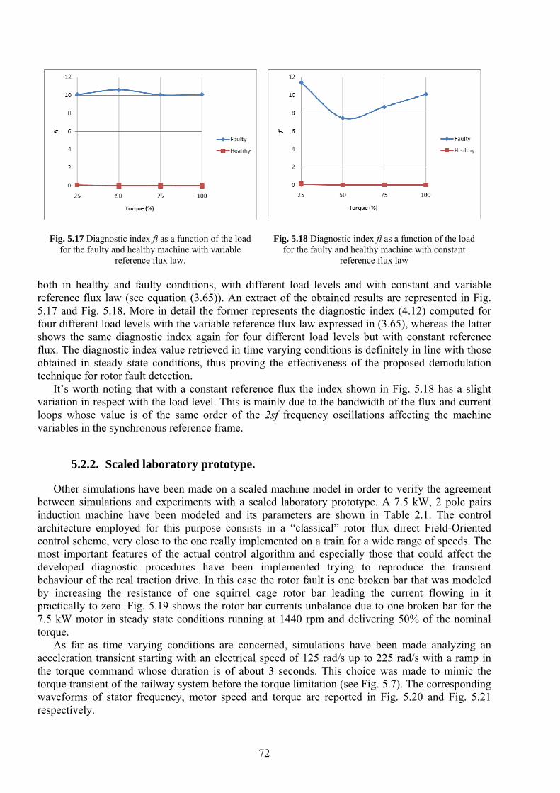
72
both in healthy and faulty conditions, with different load levels and with constant and variable reference flux law (see equation (3.65)). An extract of the obtained results are represented in Fig. 5.17 and Fig. 5.18. More in detail the former represents the diagnostic index (4.12) computed for four different load levels with the variable reference flux law expressed in (3.65), whereas the latter shows the same diagnostic index again for four different load levels but with constant reference flux. The diagnostic index value retrieved in time varying conditions is definitely in line with those obtained in steady state conditions, thus proving the effectiveness of the proposed demodulation technique for rotor fault detection.
It’s worth noting that with a constant reference flux the index shown in Fig. 5.18 has a slight variation in respect with the load level. This is mainly due to the bandwidth of the flux and current loops whose value is of the same order of the 2sf frequency oscillations affecting the machine variables in the synchronous reference frame.
5.2.2. Scaled laboratory prototype.
Other simulations have been made on a scaled machine model in order to verify the agreement between simulations and experiments with a scaled laboratory prototype. A 7.5 kW, 2 pole pairs induction machine have been modeled and its parameters are shown in Table 2.1. The control architecture employed for this purpose consists in a “classical” rotor flux direct Field-Oriented control scheme, very close to the one really implemented on a train for a wide range of speeds. The most important features of the actual control algorithm and especially those that could affect the developed diagnostic procedures have been implemented trying to reproduce the transient behaviour of the real traction drive. In this case the rotor fault is one broken bar that was modeled by increasing the resistance of one squirrel cage rotor bar leading the current flowing in it practically to zero. Fig. 5.19 shows the rotor bar currents unbalance due to one broken bar for the 7.5 kW motor in steady state conditions running at 1440 rpm and delivering 50% of the nominal torque.
As far as time varying conditions are concerned, simulations have been made analyzing an acceleration transient starting with an electrical speed of 125 rad/s up to 225 rad/s with a ramp in the torque command whose duration is of about 3 seconds. This choice was made to mimic the torque transient of the railway system before the torque limitation (see Fig. 5.7). The corresponding waveforms of stator frequency, motor speed and torque are reported in Fig. 5.20 and Fig. 5.21 respectively.
Fig. 5.17 Diagnostic index fi as a function of the load
for the faulty and healthy machine with variable reference flux law.
Fig. 5.18 Diagnostic index fi as a function of the load
for the faulty and healthy machine with constant reference flux law

73
Fig. 5.22 shows the time domain waveform of the stator currents for the same transient and for the motor running with one broken bar. Then the spectrum of their space vector in the same transient conditions for the healthy and faulty machine respectively is shown in Fig. 5.23. As before, the spectra show that no signature analysis is possible for such cases, because of the large spreading of frequency and speed. Hence the sideband components related to the faults are spread in a wide frequency range.
Fig. 5.24 shows the spectrum of the stator current space vector during the same transient after the demodulation process detailed in the previous chapter according to (4.6) and (4.7) for the faulty and healthy machine respectively with ωd =0 rad/s. Once again the proposed procedure allows to state accurately the left sideband components related to the rotor fault which is shifted to the desired prefixed zero frequency.
6 6.1 6.2 6.3 6.4 6.5 6.6 6.7 6.8 6.9 7
-400
-300
-200
-100
0
100
200
300
400
Time (s)
Bar
cur
rent
(A)
Fig. 5.19 Simulation results for the faulty 7.5 kW induction motor in steady state conditions running at 1440 rpm at
50% of the nominal torque. Rotor bar currents unbalance with 1 broken bar.
0 1 2 3 4 5 6 7120
140
160
180
200
220
240
Time (s)
Sta
tor F
requ
ency
, Ele
ctric
al S
peed
(rad
/s)
0 1 2 3 4 5 6 75
10
15
20
25
30
35
40
45
Time (s)
Torq
ue (N
m)
Fig. 5.20 Simulation results for the 7.5 kW machine. Motor speed transient for the faulty machine: stator frequency (top), electrical speed (bottom) in rad/s.
Fig. 5.21 Simulation results for the 7.5 kW machine. Torque waveforms for the faulty machine: set-point (solid line) and actual value (light grey solid line).
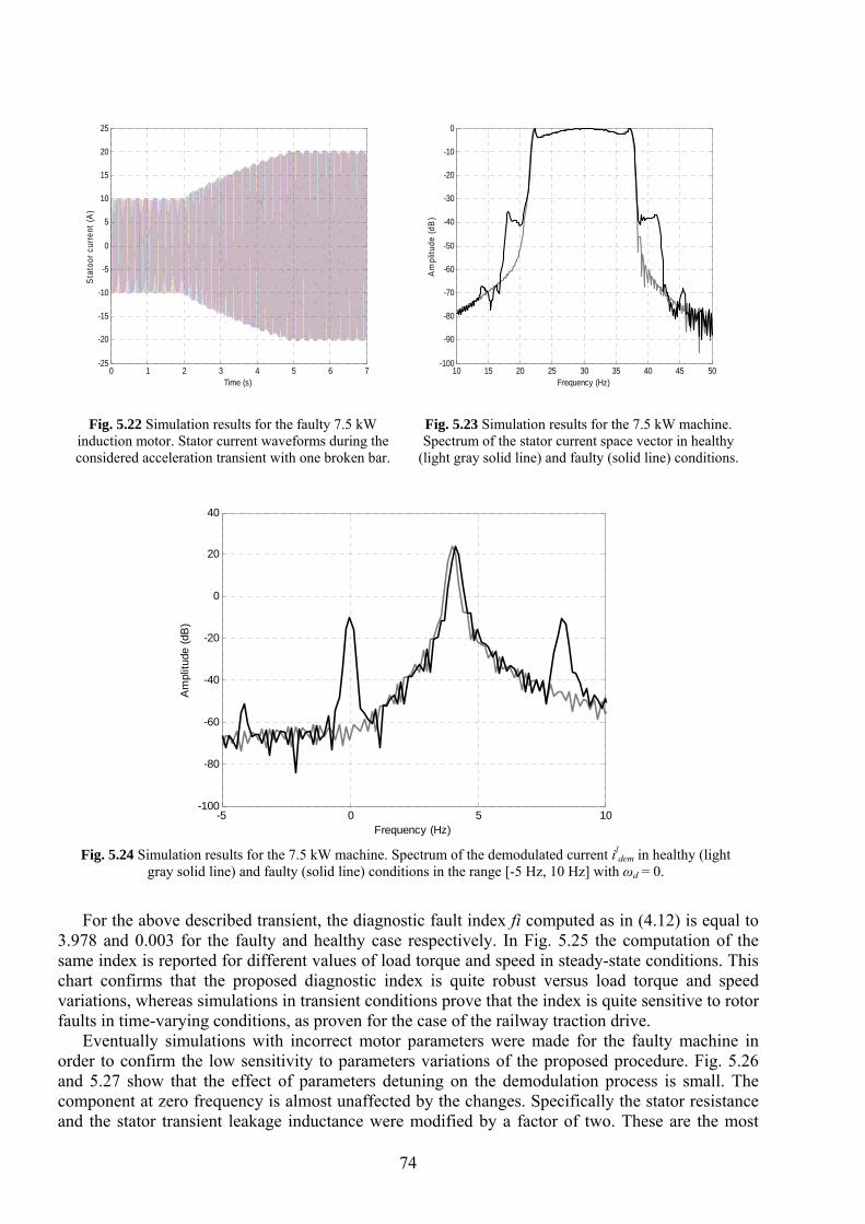
74
For the above described transient, the diagnostic fault index fi computed as in (4.12) is equal to 3.978 and 0.003 for the faulty and healthy case respectively. In Fig. 5.25 the computation of the same index is reported for different values of load torque and speed in steady-state conditions. This chart confirms that the proposed diagnostic index is quite robust versus load torque and speed variations, whereas simulations in transient conditions prove that the index is quite sensitive to rotor faults in time-varying conditions, as proven for the case of the railway traction drive.
Eventually simulations with incorrect motor parameters were made for the faulty machine in order to confirm the low sensitivity to parameters variations of the proposed procedure. Fig. 5.26 and 5.27 show that the effect of parameters detuning on the demodulation process is small. The component at zero frequency is almost unaffected by the changes. Specifically the stator resistance and the stator transient leakage inductance were modified by a factor of two. These are the most
0 1 2 3 4 5 6 7-25
-20
-15
-10
-5
0
5
10
15
20
25
Time (s)
Sta
toor
cur
rent
(A)
10 15 20 25 30 35 40 45 50-100
-90
-80
-70
-60
-50
-40
-30
-20
-10
0
Frequency (Hz)
Am
plitu
de (d
B)
Fig. 5.22 Simulation results for the faulty 7.5 kW
induction motor. Stator current waveforms during the considered acceleration transient with one broken bar.
Fig. 5.23 Simulation results for the 7.5 kW machine. Spectrum of the stator current space vector in healthy
(light gray solid line) and faulty (solid line) conditions.
-5 0 5 10-100
-80
-60
-40
-20
0
20
40
Frequency (Hz)
Am
plitu
de (d
B)
Fig. 5.24 Simulation results for the 7.5 kW machine. Spectrum of the demodulated current il
dem in healthy (light gray solid line) and faulty (solid line) conditions in the range [-5 Hz, 10 Hz] with ωd = 0.
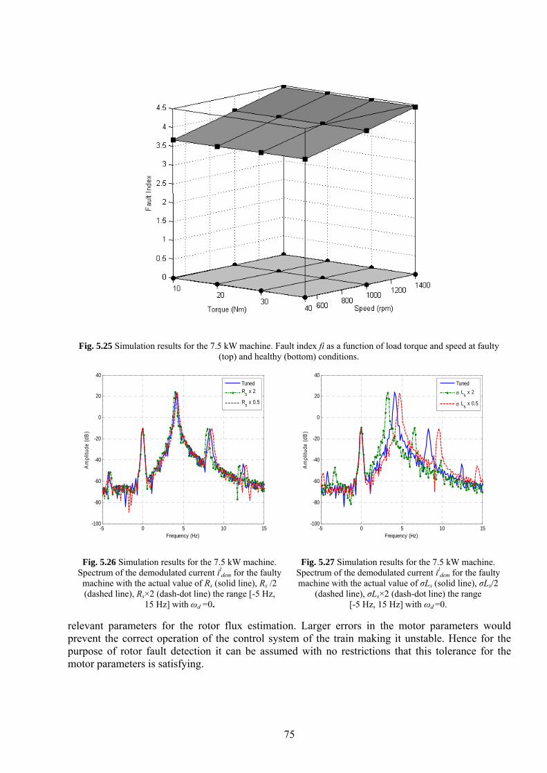
75
relevant parameters for the rotor flux estimation. Larger errors in the motor parameters would prevent the correct operation of the control system of the train making it unstable. Hence for the purpose of rotor fault detection it can be assumed with no restrictions that this tolerance for the motor parameters is satisfying.
Fig. 5.25 Simulation results for the 7.5 kW machine. Fault index fi as a function of load torque and speed at faulty
(top) and healthy (bottom) conditions.
-5 0 5 10 15-100
-80
-60
-40
-20
0
20
40
Frequency (Hz)
Am
plitu
de (d
B)
TunedRs x 2
Rs x 0.5
-5 0 5 10 15-100
-80
-60
-40
-20
0
20
40
Frequency (Hz)
Am
plitu
de (d
B)
Tunedσ Ls x 2
σ Ls x 0.5
Fig. 5.26 Simulation results for the 7.5 kW machine.
Spectrum of the demodulated current ildem for the faulty
machine with the actual value of Rs (solid line), Rs /2 (dashed line), Rs×2 (dash-dot line) the range [-5 Hz,
15 Hz] with ωd =0.
Fig. 5.27 Simulation results for the 7.5 kW machine.
Spectrum of the demodulated current ildem for the faulty
machine with the actual value of σLs (solid line), σLs/2 (dashed line), σLs×2 (dash-dot line) the range
[-5 Hz, 15 Hz] with ωd =0.
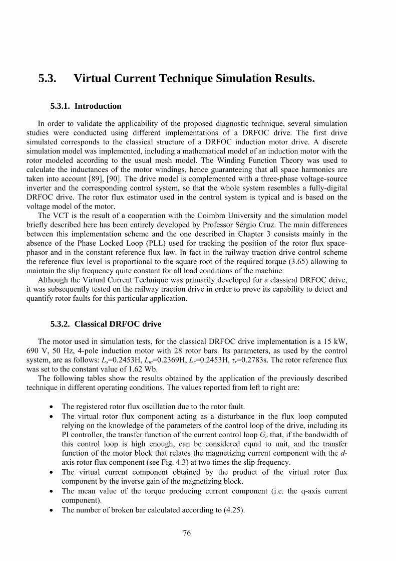
76
5.3. Virtual Current Technique Simulation Results.
5.3.1. Introduction
In order to validate the applicability of the proposed diagnostic technique, several simulation studies were conducted using different implementations of a DRFOC drive. The first drive simulated corresponds to the classical structure of a DRFOC induction motor drive. A discrete simulation model was implemented, including a mathematical model of an induction motor with the rotor modeled according to the usual mesh model. The Winding Function Theory was used to calculate the inductances of the motor windings, hence guaranteeing that all space harmonics are taken into account [89], [90]. The drive model is complemented with a three-phase voltage-source inverter and the corresponding control system, so that the whole system resembles a fully-digital DRFOC drive. The rotor flux estimator used in the control system is typical and is based on the voltage model of the motor.
The VCT is the result of a cooperation with the Coimbra University and the simulation model briefly described here has been entirely developed by Professor Sérgio Cruz. The main differences between this implementation scheme and the one described in Chapter 3 consists mainly in the absence of the Phase Locked Loop (PLL) used for tracking the position of the rotor flux space-phasor and in the constant reference flux law. In fact in the railway traction drive control scheme the reference flux level is proportional to the square root of the required torque (3.65) allowing to maintain the slip frequency quite constant for all load conditions of the machine.
Although the Virtual Current Technique was primarily developed for a classical DRFOC drive, it was subsequently tested on the railway traction drive in order to prove its capability to detect and quantify rotor faults for this particular application.
5.3.2. Classical DRFOC drive
The motor used in simulation tests, for the classical DRFOC drive implementation is a 15 kW, 690 V, 50 Hz, 4-pole induction motor with 28 rotor bars. Its parameters, as used by the control system, are as follows: Ls=0.2453H, Lm=0.2369H, Lr=0.2453H, τr=0.2783s. The rotor reference flux was set to the constant value of 1.62 Wb.
The following tables show the results obtained by the application of the previously described technique in different operating conditions. The values reported from left to right are:
• The registered rotor flux oscillation due to the rotor fault. • The virtual rotor flux component acting as a disturbance in the flux loop computed
relying on the knowledge of the parameters of the control loop of the drive, including its PI controller, the transfer function of the current control loop Gc that, if the bandwidth of this control loop is high enough, can be considered equal to unit, and the transfer function of the motor block that relates the magnetizing current component with the d-axis rotor flux component (see Fig. 4.3) at two times the slip frequency.
• The virtual current component obtained by the product of the virtual rotor flux component by the inverse gain of the magnetizing block.
• The mean value of the torque producing current component (i.e. the q-axis current component).
• The number of broken bar calculated according to (4.25).
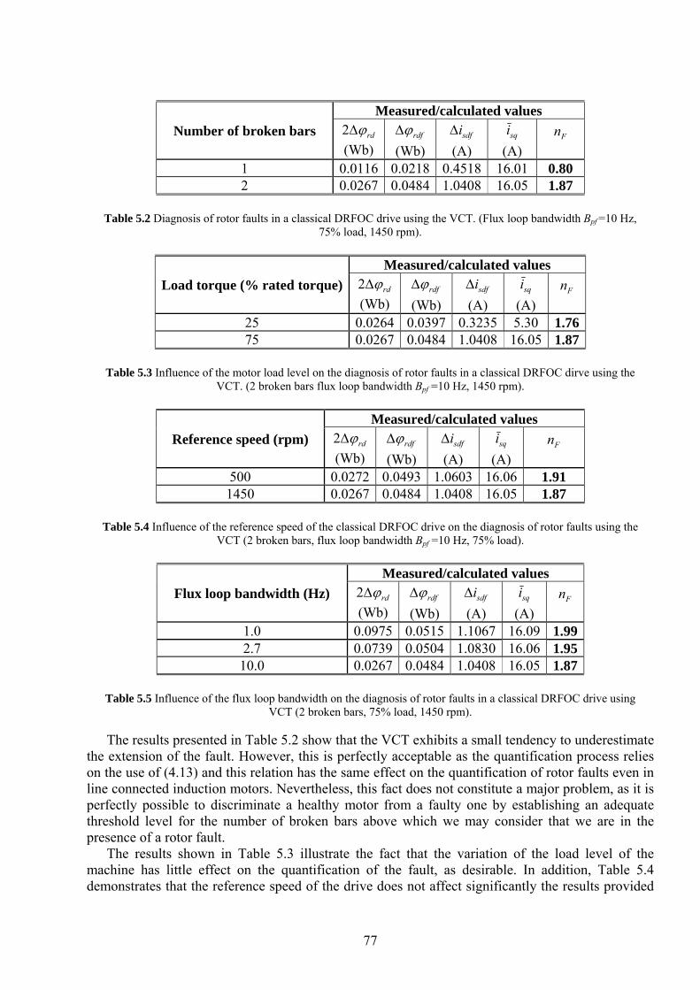
77
The results presented in Table 5.2 show that the VCT exhibits a small tendency to underestimate the extension of the fault. However, this is perfectly acceptable as the quantification process relies on the use of (4.13) and this relation has the same effect on the quantification of rotor faults even in line connected induction motors. Nevertheless, this fact does not constitute a major problem, as it is perfectly possible to discriminate a healthy motor from a faulty one by establishing an adequate threshold level for the number of broken bars above which we may consider that we are in the presence of a rotor fault.
The results shown in Table 5.3 illustrate the fact that the variation of the load level of the machine has little effect on the quantification of the fault, as desirable. In addition, Table 5.4 demonstrates that the reference speed of the drive does not affect significantly the results provided
Number of broken bars Measured/calculated values
rdϕΔ2 (Wb)
rdfϕΔ (Wb)
sdfiΔ (A)
sqi (A)
Fn
1 0.0116 0.0218 0.4518 16.01 0.80 2 0.0267 0.0484 1.0408 16.05 1.87
Table 5.2 Diagnosis of rotor faults in a classical DRFOC drive using the VCT. (Flux loop bandwidth Bpf =10 Hz,
75% load, 1450 rpm).
Load torque (% rated torque)Measured/calculated values rdϕΔ2
(Wb) rdfϕΔ
(Wb) sdfiΔ
(A) sqi
(A) Fn
25 0.0264 0.0397 0.3235 5.30 1.7675 0.0267 0.0484 1.0408 16.05 1.87
Table 5.3 Influence of the motor load level on the diagnosis of rotor faults in a classical DRFOC dirve using the
VCT. (2 broken bars flux loop bandwidth Bpf =10 Hz, 1450 rpm).
Reference speed (rpm) Measured/calculated values
rdϕΔ2 (Wb)
rdfϕΔ (Wb)
sdfiΔ (A)
sqi (A)
Fn
500 0.0272 0.0493 1.0603 16.06 1.91 1450 0.0267 0.0484 1.0408 16.05 1.87
Table 5.4 Influence of the reference speed of the classical DRFOC drive on the diagnosis of rotor faults using the
VCT (2 broken bars, flux loop bandwidth Bpf =10 Hz, 75% load).
Flux loop bandwidth (Hz) Measured/calculated values rdϕΔ2
(Wb) rdfϕΔ
(Wb) sdfiΔ
(A) sqi
(A) Fn
1.0 0.0975 0.0515 1.1067 16.09 1.99 2.7 0.0739 0.0504 1.0830 16.06 1.95 10.0 0.0267 0.0484 1.0408 16.05 1.87
Table 5.5 Influence of the flux loop bandwidth on the diagnosis of rotor faults in a classical DRFOC drive using
VCT (2 broken bars, 75% load, 1450 rpm).
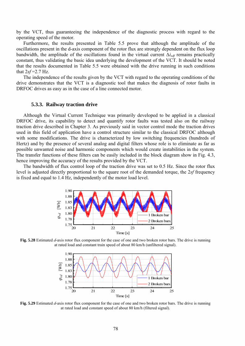
78
by the VCT, thus guaranteeing the independence of the diagnostic process with regard to the operating speed of the motor.
Furthermore, the results presented in Table 5.5 prove that although the amplitude of the oscillations present in the d-axis component of the rotor flux are strongly dependent on the flux loop bandwidth, the amplitude of the oscillations found in the virtual current Δisdf remains practically constant, thus validating the basic idea underlying the development of the VCT. It should be noted that the results documented in Table 5.5 were obtained with the drive running in such conditions that 2sf =2.7 Hz.
The independence of the results given by the VCT with regard to the operating conditions of the drive demonstrates that the VCT is a diagnostic tool that makes the diagnosis of rotor faults in DRFOC drives as easy as in the case of a line connected motor.
5.3.3. Railway traction drive
Although the Virtual Current Technique was primarily developed to be applied in a classical DRFOC drive, its capability to detect and quantify rotor faults was tested also on the railway traction drive described in Chapter 3. As previously said in vector control mode the traction drives used in this field of application have a control structure similar to the classical DRFOC although with some modifications. The drive is characterized by low switching frequencies (hundreds of Hertz) and by the presence of several analog and digital filters whose role is to eliminate as far as possible unwanted noise and harmonic components which would create instabilities in the system. The transfer functions of these filters can be easily included in the block diagram show in Fig. 4.3, hence improving the accuracy of the results provided by the VCT.
The bandwidth of flux control loop of the traction drive was set to 0.5 Hz. Since the rotor flux level is adjusted directly proportional to the square root of the demanded torque, the 2sf frequency is fixed and equal to 1.4 Hz, independently of the motor load level.
20 21 22 23 24 25Time [s]
1.751.781.801.831.851.881.90
1 Broken bar2 Broken bars
ψ dr[W
b]
Fig. 5.28 Estimated d-axis rotor flux component for the case of one and two broken rotor bars. The drive is running at rated load and constant train speed of about 80 km/h (unfiltered signal).
20 21 22 23 24 25Time [s]
1.751.781.801.831.851.881.90
1 Broken bar2 Broken bars
ψ d r[W
b]
Fig. 5.29 Estimated d-axis rotor flux component for the case of one and two broken rotor bars. The drive is running at rated load and constant speed of about 80 km/h (filtered signal).
φ rd
[Wb]
φ r
d [W
b]
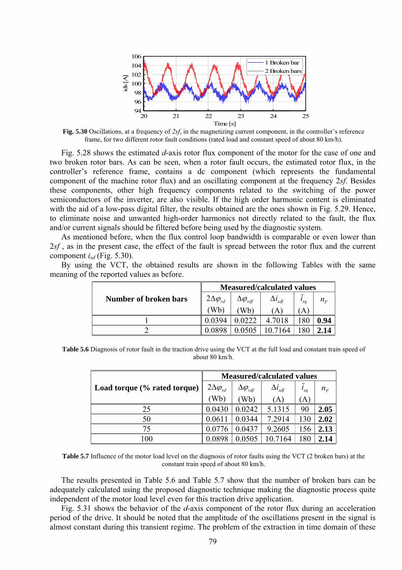
79
Fig. 5.28 shows the estimated d-axis rotor flux component of the motor for the case of one and two broken rotor bars. As can be seen, when a rotor fault occurs, the estimated rotor flux, in the controller’s reference frame, contains a dc component (which represents the fundamental component of the machine rotor flux) and an oscillating component at the frequency 2sf. Besides these components, other high frequency components related to the switching of the power semiconductors of the inverter, are also visible. If the high order harmonic content is eliminated with the aid of a low-pass digital filter, the results obtained are the ones shown in Fig. 5.29. Hence, to eliminate noise and unwanted high-order harmonics not directly related to the fault, the flux and/or current signals should be filtered before being used by the diagnostic system.
As mentioned before, when the flux control loop bandwidth is comparable or even lower than 2sf , as in the present case, the effect of the fault is spread between the rotor flux and the current component isd (Fig. 5.30).
By using the VCT, the obtained results are shown in the following Tables with the same meaning of the reported values as before.
The results presented in Table 5.6 and Table 5.7 show that the number of broken bars can be adequately calculated using the proposed diagnostic technique making the diagnostic process quite independent of the motor load level even for this traction drive application.
Fig. 5.31 shows the behavior of the d-axis component of the rotor flux during an acceleration period of the drive. It should be noted that the amplitude of the oscillations present in the signal is almost constant during this transient regime. The problem of the extraction in time domain of these
20 21 22 23 24 25Time [s]
949698
100102104106
ids [
A]
1 Broken bar2 Broken bars
Fig. 5.30 Oscillations, at a frequency of 2sf, in the magnetizing current component, in the controller’s reference
frame, for two different rotor fault conditions (rated load and constant speed of about 80 km/h).
Number of broken bars Measured/calculated values rdϕΔ2
(Wb) rdfϕΔ
(Wb) sdfiΔ
(A) sqi
(A) Fn
1 0.0394 0.0222 4.7018 180 0.94 2 0.0898 0.0505 10.7164 180 2.14
Table 5.6 Diagnosis of rotor fault in the traction drive using the VCT at the full load and constant train speed of
about 80 km/h.
Load torque (% rated torque)Measured/calculated values rdϕΔ2
(Wb) rdfϕΔ
(Wb) sdfiΔ
(A) sqi
(A) Fn
25 0.0430 0.0242 5.1315 90 2.0550 0.0611 0.0344 7.2914 130 2.0275 0.0776 0.0437 9.2605 156 2.13100 0.0898 0.0505 10.7164 180 2.14
Table 5.7 Influence of the motor load level on the diagnosis of rotor faults using the VCT (2 broken bars) at the
constant train speed of about 80 km/h.
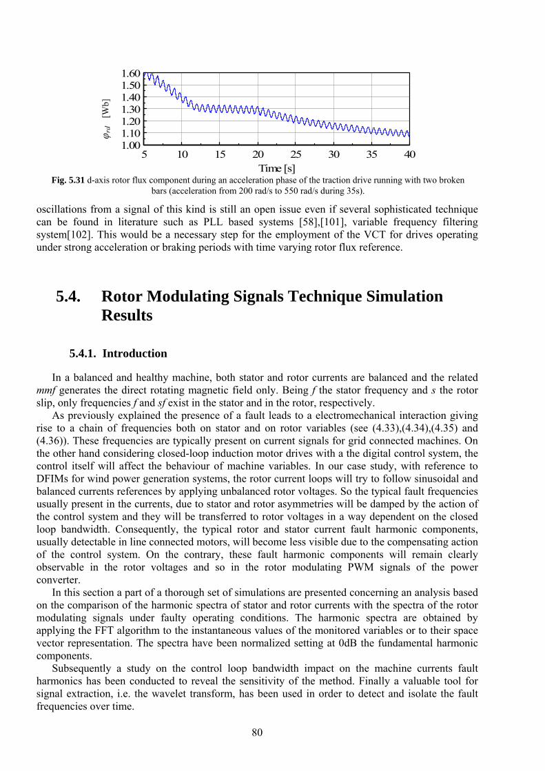
80
oscillations from a signal of this kind is still an open issue even if several sophisticated technique can be found in literature such as PLL based systems [58],[101], variable frequency filtering system[102]. This would be a necessary step for the employment of the VCT for drives operating under strong acceleration or braking periods with time varying rotor flux reference.
5.4. Rotor Modulating Signals Technique Simulation Results
5.4.1. Introduction
In a balanced and healthy machine, both stator and rotor currents are balanced and the related mmf generates the direct rotating magnetic field only. Being f the stator frequency and s the rotor slip, only frequencies f and sf exist in the stator and in the rotor, respectively.
As previously explained the presence of a fault leads to a electromechanical interaction giving rise to a chain of frequencies both on stator and on rotor variables (see (4.33),(4.34),(4.35) and (4.36)). These frequencies are typically present on current signals for grid connected machines. On the other hand considering closed-loop induction motor drives with a the digital control system, the control itself will affect the behaviour of machine variables. In our case study, with reference to DFIMs for wind power generation systems, the rotor current loops will try to follow sinusoidal and balanced currents references by applying unbalanced rotor voltages. So the typical fault frequencies usually present in the currents, due to stator and rotor asymmetries will be damped by the action of the control system and they will be transferred to rotor voltages in a way dependent on the closed loop bandwidth. Consequently, the typical rotor and stator current fault harmonic components, usually detectable in line connected motors, will become less visible due to the compensating action of the control system. On the contrary, these fault harmonic components will remain clearly observable in the rotor voltages and so in the rotor modulating PWM signals of the power converter.
In this section a part of a thorough set of simulations are presented concerning an analysis based on the comparison of the harmonic spectra of stator and rotor currents with the spectra of the rotor modulating signals under faulty operating conditions. The harmonic spectra are obtained by applying the FFT algorithm to the instantaneous values of the monitored variables or to their space vector representation. The spectra have been normalized setting at 0dB the fundamental harmonic components.
Subsequently a study on the control loop bandwidth impact on the machine currents fault harmonics has been conducted to reveal the sensitivity of the method. Finally a valuable tool for signal extraction, i.e. the wavelet transform, has been used in order to detect and isolate the fault frequencies over time.
5 10 15 20 25 30 35 40Time [s]
1.001.101.201.301.401.501.60
ψ dr[ W
b]
Fig. 5.31 d-axis rotor flux component during an acceleration phase of the traction drive running with two broken
bars (acceleration from 200 rad/s to 550 rad/s during 35s).
φ rd
[Wb]
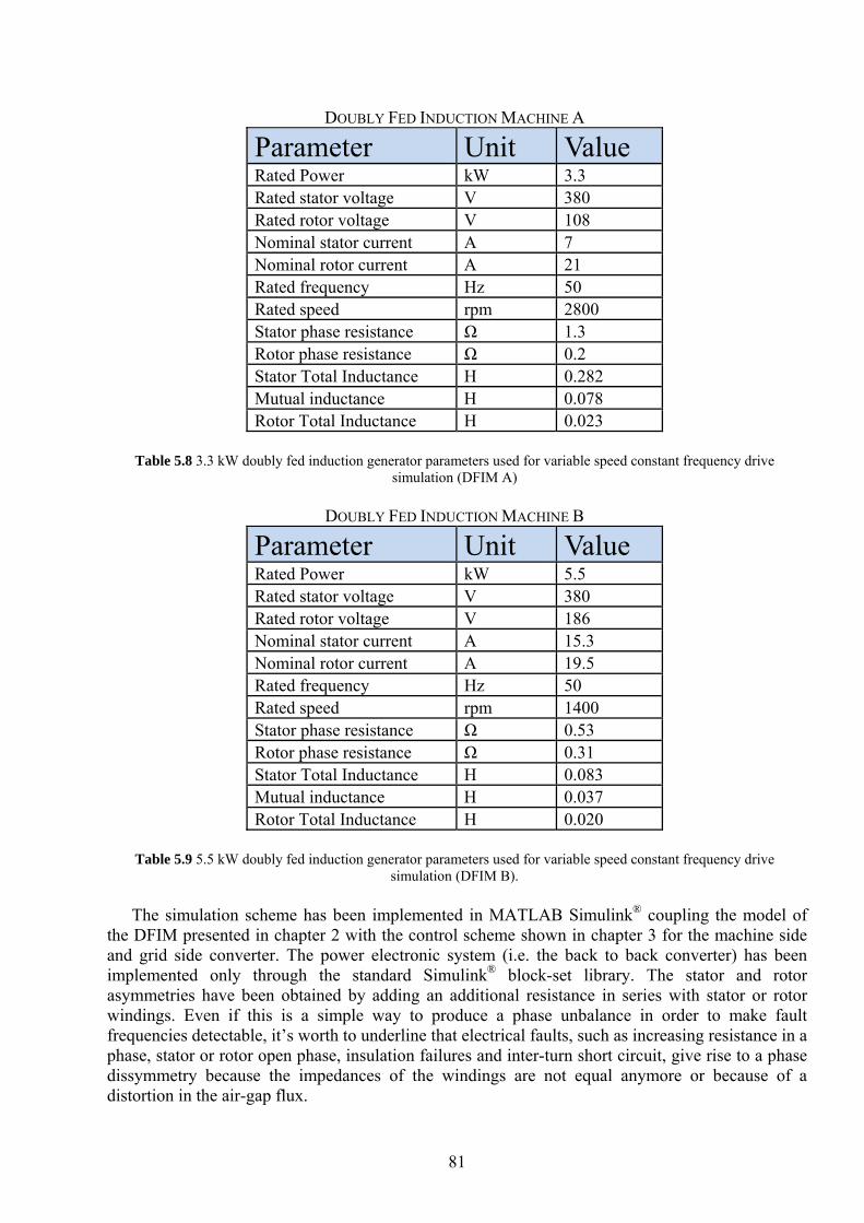
81
The simulation scheme has been implemented in MATLAB Simulink® coupling the model of the DFIM presented in chapter 2 with the control scheme shown in chapter 3 for the machine side and grid side converter. The power electronic system (i.e. the back to back converter) has been implemented only through the standard Simulink® block-set library. The stator and rotor asymmetries have been obtained by adding an additional resistance in series with stator or rotor windings. Even if this is a simple way to produce a phase unbalance in order to make fault frequencies detectable, it’s worth to underline that electrical faults, such as increasing resistance in a phase, stator or rotor open phase, insulation failures and inter-turn short circuit, give rise to a phase dissymmetry because the impedances of the windings are not equal anymore or because of a distortion in the air-gap flux.
DOUBLY FED INDUCTION MACHINE A
Parameter Unit Value Rated Power kW 3.3 Rated stator voltage V 380 Rated rotor voltage V 108 Nominal stator current A 7 Nominal rotor current A 21 Rated frequency Hz 50 Rated speed rpm 2800 Stator phase resistance Ω 1.3 Rotor phase resistance Ω 0.2 Stator Total Inductance H 0.282 Mutual inductance H 0.078 Rotor Total Inductance H 0.023
Table 5.8 3.3 kW doubly fed induction generator parameters used for variable speed constant frequency drive
simulation (DFIM A)
DOUBLY FED INDUCTION MACHINE B
Parameter Unit Value Rated Power kW 5.5 Rated stator voltage V 380 Rated rotor voltage V 186 Nominal stator current A 15.3 Nominal rotor current A 19.5 Rated frequency Hz 50 Rated speed rpm 1400 Stator phase resistance Ω 0.53 Rotor phase resistance Ω 0.31 Stator Total Inductance H 0.083 Mutual inductance H 0.037 Rotor Total Inductance H 0.020
Table 5.9 5.5 kW doubly fed induction generator parameters used for variable speed constant frequency drive
simulation (DFIM B).
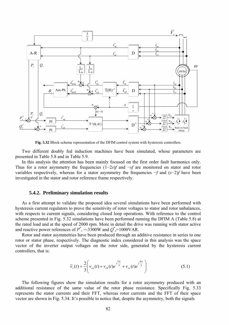
82
Two different doubly fed induction machines have been simulated, whose parameters are presented in Table 5.8 and in Table 5.9.
In this analysis the attention has been mainly focused on the first order fault harmonics only. Thus for a rotor asymmetry the frequencies (1−2s)f and −sf are monitored on stator and rotor variables respectively, whereas for a stator asymmetry the frequencies −f and (s−2)f have been investigated in the stator and rotor reference frame respectively.
5.4.2. Preliminary simulation results
As a first attempt to validate the proposed idea several simulations have been performed with hysteresis current regulators to prove the sensitivity of rotor voltages to stator and rotor unbalances, with respects to current signals, considering closed loop operations. With reference to the control scheme presented in Fig. 5.32 simulations have been performed running the DFIM A (Table 5.8) at the rated load and at the speed of 2000 rpm. More in detail the drive was running with stator active and reactive power references of P*
s =-3300W and Q*s=1000VAR.
Rotor and stator asymmetries have been produced through an additive resistance in series to one rotor or stator phase, respectively. The diagnostic index considered in this analysis was the space vector of the inverter output voltages on the rotor side, generated by the hysteresis current controllers, that is:
⎟⎟⎠
⎞⎜⎜⎝
⎛++= 3
43
2
)()()(32)(
ππ j
rc
j
rbrar etvetvtvtv (5.1)
The following figures show the simulation results for a rotor asymmetry produced with an
additional resistance of the same value of the rotor phase resistance. Specifically Fig. 5.33 represents the stator currents and their FFT, whereas rotor currents and the FFT of their space vector are shown in Fig. 5.34. It’s possible to notice that, despite the asymmetry, both the signals
aribricri
asibsicsi
s1
rrqirrdi
ssqissdi
srqisrdi
smsqismsdiθ
( )s θθ −
*i
*i
*sP
*s
A-R
sP sQ
sV
sP s+
+
+
+ +
+ +
DFIM
Back-to-backPWM
D
DT(θ)-1
T-1(θ -θ )
ω
Am-Ph
PI
PIQ
Q
θ
D-1
+
+
+
LLL
L
rq
rd
s smm
s
23
s
rav
rbvrcv
Fig. 5.32 Block-scheme representation of the DFIM control system with hysteresis controllers.
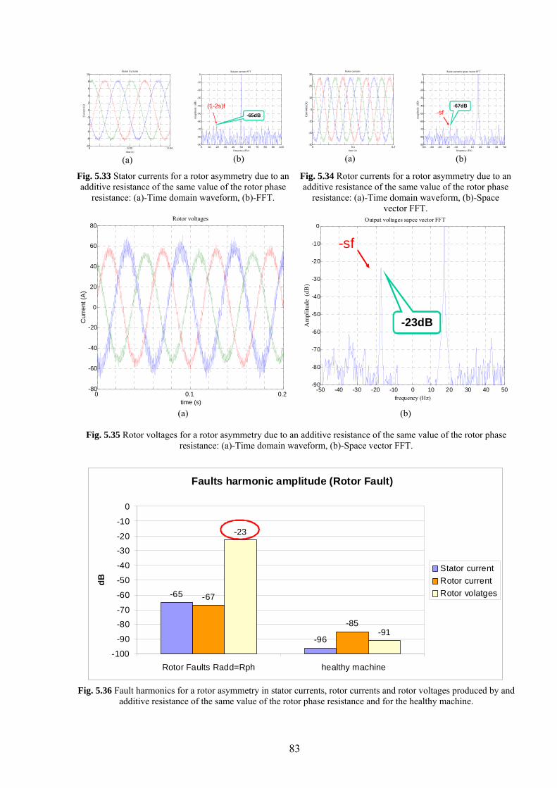
83
0 0.02 0.04-10
-8
-6
-4
-2
0
2
4
6
8
10
time (s)
Cur
rent
(A)
Stator Currents
(a)
0 10 20 30 40 50 60 70 80 90 100-90
-80
-70
-60
-50
-40
-30
-20
-10
0Satator current FFT
Am
plitu
de (
dB)
frequency (Hz)
-65dB
(1-2s)f
(b)
0 0,1 0,2-30
-20
-10
0
10
20
30
time (s)
Cur
rent
s (A
)
Rotor currents
(a)
-50 -40 -30 -20 -10 0 10 20 30 40 50-90
-80
-70
-60
-50
-40
-30
-20
-10
0Rotor currents space vector FFT
Am
plitu
de (
dB)
frequency (Hz)
-67dB-sf
(b)
Fig. 5.33 Stator currents for a rotor asymmetry due to an additive resistance of the same value of the rotor phase
resistance: (a)-Time domain waveform, (b)-FFT.
Fig. 5.34 Rotor currents for a rotor asymmetry due to an additive resistance of the same value of the rotor phase
resistance: (a)-Time domain waveform, (b)-Space vector FFT.
0 0.1 0.2-80
-60
-40
-20
0
20
40
60
80
time (s)
Cur
rent
(A)
Rotor voltages
-50 -40 -30 -20 -10 0 10 20 30 40 50-90
-80
-70
-60
-50
-40
-30
-20
-10
0Output voltages sapce vector FFT
Am
plitu
de (
dB)
frequency (Hz)
-sf
-23dB
(a) (b)
Fig. 5.35 Rotor voltages for a rotor asymmetry due to an additive resistance of the same value of the rotor phase resistance: (a)-Time domain waveform, (b)-Space vector FFT.
Faults harmonic amplitude (Rotor Fault)
-65
-96
-67
-85
-23
-91
-100
-90
-80
-70
-60
-50
-40
-30
-20
-10
0
Rotor Faults Radd=Rph healthy machine
dB
Stator currentRotor currentRotor volatges
Fig. 5.36 Fault harmonics for a rotor asymmetry in stator currents, rotor currents and rotor voltages produced by and
additive resistance of the same value of the rotor phase resistance and for the healthy machine.
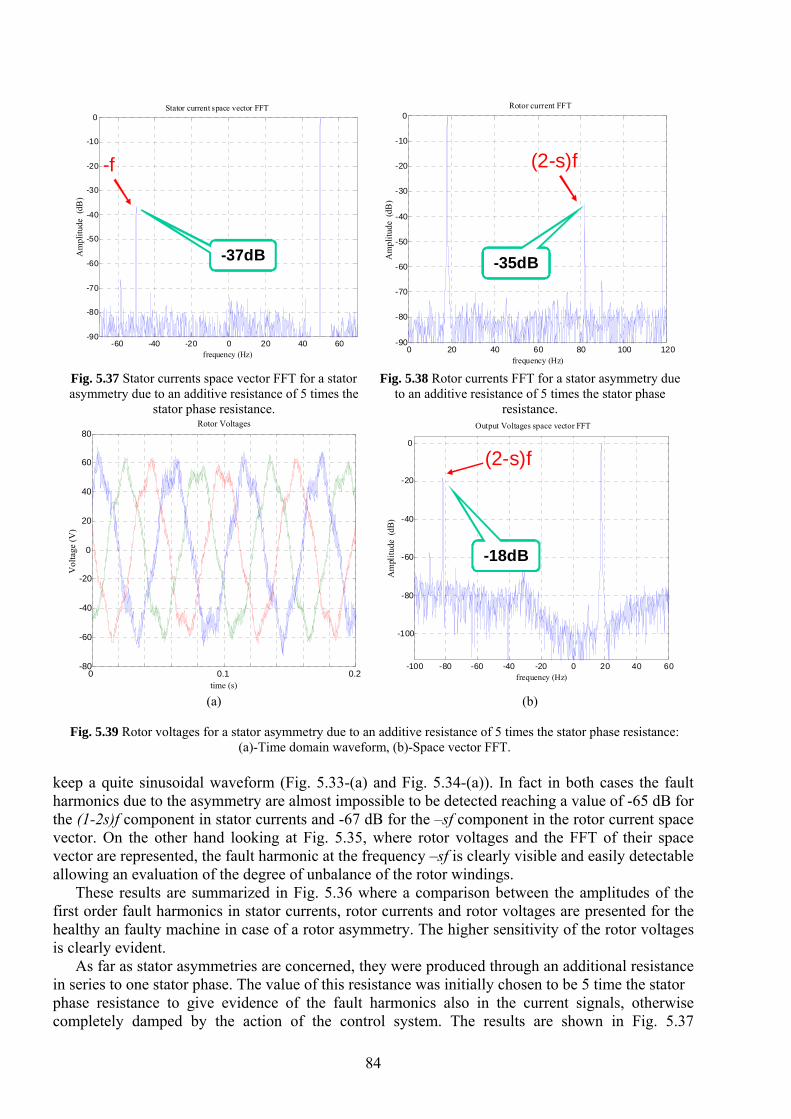
84
keep a quite sinusoidal waveform (Fig. 5.33-(a) and Fig. 5.34-(a)). In fact in both cases the fault harmonics due to the asymmetry are almost impossible to be detected reaching a value of -65 dB for the (1-2s)f component in stator currents and -67 dB for the –sf component in the rotor current space vector. On the other hand looking at Fig. 5.35, where rotor voltages and the FFT of their space vector are represented, the fault harmonic at the frequency –sf is clearly visible and easily detectable allowing an evaluation of the degree of unbalance of the rotor windings.
These results are summarized in Fig. 5.36 where a comparison between the amplitudes of the first order fault harmonics in stator currents, rotor currents and rotor voltages are presented for the healthy an faulty machine in case of a rotor asymmetry. The higher sensitivity of the rotor voltages is clearly evident.
As far as stator asymmetries are concerned, they were produced through an additional resistance in series to one stator phase. The value of this resistance was initially chosen to be 5 time the stator phase resistance to give evidence of the fault harmonics also in the current signals, otherwise completely damped by the action of the control system. The results are shown in Fig. 5.37
-60 -40 -20 0 20 40 60-90
-80
-70
-60
-50
-40
-30
-20
-10
0Stator current space vector FFT
Am
plitu
de (
dB)
frequency (Hz)
-f
-37dB
0 20 40 60 80 100 120
-90
-80
-70
-60
-50
-40
-30
-20
-10
0Rotor current FFT
Am
plitu
de (
dB)
frequency (Hz)
(2-s)f
-35dB
Fig. 5.37 Stator currents space vector FFT for a stator asymmetry due to an additive resistance of 5 times the
stator phase resistance.
Fig. 5.38 Rotor currents FFT for a stator asymmetry due to an additive resistance of 5 times the stator phase
resistance.
0 0.1 0.2-80
-60
-40
-20
0
20
40
60
80
time (s)
Vol
tage
(V)
Rotor Voltages
-100 -80 -60 -40 -20 0 20 40 60
-100
-80
-60
-40
-20
0
Output Voltages space vector FFT
Am
plitu
de (
dB)
frequency (Hz)
(2-s)f
-18dB
(a) (b)
Fig. 5.39 Rotor voltages for a stator asymmetry due to an additive resistance of 5 times the stator phase resistance: (a)-Time domain waveform, (b)-Space vector FFT.
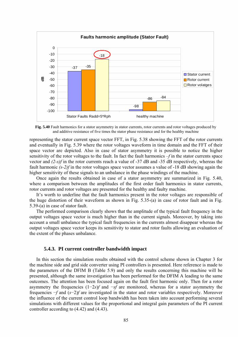
85
representing the stator current space vector FFT, in Fig. 5.38 showing the FFT of the rotor currents and eventually in Fig. 5.39 where the rotor voltages waveform in time domain and the FFT of their space vector are depicted. Also in case of stator asymmetry it is possible to notice the higher sensitivity of the rotor voltages to the fault. In fact the fault harmonics –f in the stator currents space vector and (2-s)f in the rotor currents reach a value of -37 dB and -35 dB respectively, whereas the fault harmonic (s-2)f in the rotor voltages space vector assumes a value of -18 dB showing again the higher sensitivity of these signals to an unbalance in the phase windings of the machine.
Once again the results obtained in case of a stator asymmetry are summarized in Fig. 5.40, where a comparison between the amplitudes of the first order fault harmonics in stator currents, rotor currents and rotor voltages are presented for the healthy and faulty machine.
It’s worth to underline that the fault harmonics present in the rotor voltages are responsible of the huge distortion of their waveform as shown in Fig. 5.35-(a) in case of rotor fault and in Fig. 5.39-(a) in case of stator fault.
The performed comparison clearly shows that the amplitude of the typical fault frequency in the output voltages space vector is much higher than in the current signals. Moreover, by taking into account a small unbalance the typical fault frequencies in the currents almost disappear whereas the output voltages space vector keeps its sensitivity to stator and rotor faults allowing an evaluation of the extent of the phases unbalance.
5.4.3. PI current controller bandwidth impact
In this section the simulation results obtained with the control scheme shown in Chapter 3 for the machine side and grid side converter using PI controllers is presented. Here reference is made to the parameters of the DFIM B (Table 5.9) and only the results concerning this machine will be presented, although the same investigation has been performed for the DFIM A leading to the same outcomes. The attention has been focused again on the fault first harmonic only. Then for a rotor asymmetry the frequencies (1−2s)f and −sf are monitored, whereas for a stator asymmetry the frequencies −f and (s−2)f are investigated in the stator and rotor variables respectively. Moreover the influence of the current control loop bandwidth has been taken into account performing several simulations with different values for the proportional and integral gain parameters of the PI current controller according to (4.42) and (4.43).
Faults harmonic amplitude (Stator Fault)
-37
-98
-35
-86
-18
-84
-100
-90
-80
-70
-60
-50
-40
-30
-20
-10
0
Stator Faults Radd=5*Rph healthy machine
dB
Stator currentRotor currentRotor volatges
Fig. 5.40 Fault harmonics for a stator asymmetry in stator currents, rotor currents and rotor voltages produced by
and additive resistance of five times the stator phase resistance and for the healthy machine
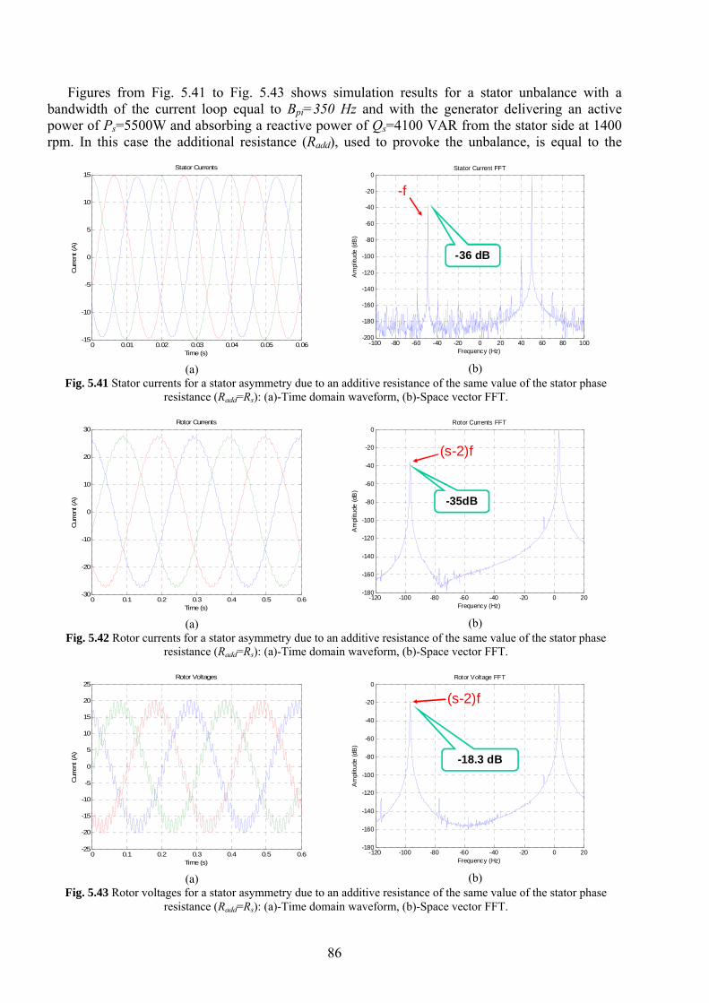
86
Figures from Fig. 5.41 to Fig. 5.43 shows simulation results for a stator unbalance with a bandwidth of the current loop equal to Bpi=350 Hz and with the generator delivering an active power of Ps=5500W and absorbing a reactive power of Qs=4100 VAR from the stator side at 1400 rpm. In this case the additional resistance (Radd), used to provoke the unbalance, is equal to the
0 0.01 0.02 0.03 0.04 0.05 0.06-15
-10
-5
0
5
10
15Stator Currents
Time (s)
Cur
rent
(A)
(a)
-100 -80 -60 -40 -20 0 20 40 60 80 100-200
-180
-160
-140
-120
-100
-80
-60
-40
-20
0Stator Current FFT
Frequency (Hz)A
mpl
itude
(dB
)
-36 dB
-f
(b)
Fig. 5.41 Stator currents for a stator asymmetry due to an additive resistance of the same value of the stator phase resistance (Radd=Rs): (a)-Time domain waveform, (b)-Space vector FFT.
0 0.1 0.2 0.3 0.4 0.5 0.6-30
-20
-10
0
10
20
30Rotor Currents
Time (s)
Cur
rent
(A)
(a)
-120 -100 -80 -60 -40 -20 0 20-180
-160
-140
-120
-100
-80
-60
-40
-20
0Rotor Currents FFT
Frequency (Hz)
Am
plitu
de (d
B)
(s-2)f
-35dB
(b)
Fig. 5.42 Rotor currents for a stator asymmetry due to an additive resistance of the same value of the stator phase resistance (Radd=Rs): (a)-Time domain waveform, (b)-Space vector FFT.
0 0.1 0.2 0.3 0.4 0.5 0.6-25
-20
-15
-10
-5
0
5
10
15
20
25Rotor Voltages
Time (s)
Cur
rent
(A)
(a)
-120 -100 -80 -60 -40 -20 0 20-180
-160
-140
-120
-100
-80
-60
-40
-20
0Rotor Voltage FFT
Frequency (Hz)
Am
plitu
de (d
B)
(s-2)f
-18.3 dB
(b)
Fig. 5.43 Rotor voltages for a stator asymmetry due to an additive resistance of the same value of the stator phase resistance (Radd=Rs): (a)-Time domain waveform, (b)-Space vector FFT.
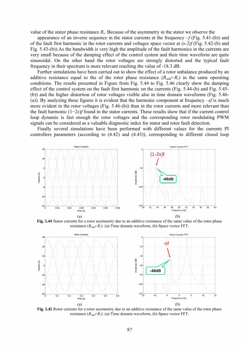
87
value of the stator phase resistance Rs. Because of the asymmetry in the stator we observe the appearance of an inverse sequence in the stator currents at the frequency –f (Fig. 5.41-(b)) and
of the fault first harmonic in the rotor currents and voltages space vector at (s-2)f (Fig. 5.42-(b) and Fig. 5.43-(b)).As the bandwidth is very high the amplitude of the fault harmonics in the currents are very small because of the damping effect of the control system and their time waveform are quite sinusoidal. On the other hand the rotor voltages are strongly distorted and the typical fault frequency in their spectrum is more relevant reaching the value of -18.3 dB.
Further simulations have been carried out to show the effect of a rotor unbalance produced by an additive resistance equal to the of the rotor phase resistance (Radd=Rr) in the same operating conditions. The results presented in Figure from Fig. 5.44 to Fig. 5.46 clearly show the damping effect of the control system on the fault first harmonic on the currents (Fig. 5.44-(b) and Fig. 5.45-(b)) and the higher distortion of rotor voltages visible also in time domain waveforms (Fig. 5.46-(a)). By analyzing these figures it is evident that the harmonic component at frequency –sf is much more evident in the rotor voltages (Fig. 5.46-(b)) than in the rotor currents and more relevant than the fault harmonic (1−2s)f found in the stator currents. These results show that if the current control loop dynamic is fast enough the rotor voltages and the corresponding rotor modulating PWM signals can be considered as a valuable diagnostic index for stator and rotor fault detection.
Finally several simulations have been performed with different values for the currents PI controllers parameters (according to (4.42) and (4.43)), corresponding to different closed loop
0 0.01 0.02 0.03 0.04 0.05 0.06-15
-10
-5
0
5
10
15Stator Currents
Time (s)
Cur
rent
(A)
(a)
40 42 44 46 48 50 52 54 56 58 60-150
-100
-50
0Stator Current FFT
Frequency (Hz)
Am
plitu
de (d
B)
(1-2s)f
-49dB
(b)
Fig. 5.44 Stator currents for a rotor asymmetry due to an additive resistance of the same value of the rotor phase resistance (Radd=Rr): (a)-Time domain waveform, (b)-Space vector FFT.
0 0.1 0.2 0.3 0.4 0.5 0.6-30
-20
-10
0
10
20
30Rotor Currents
Time (s)
Cur
rent
(A)
(a)
-15 -10 -5 0 5 10 15-120
-100
-80
-60
-40
-20
0Rotor Currents FFT
Frequency (Hz)
Am
plitu
de (d
B)
-sf
-48dB
(b)
Fig. 5.45 Rotor currents for a rotor asymmetry due to an additive resistance of the same value of the rotor phase resistance (Radd=Rr): (a)-Time domain waveform, (b)-Space vector FFT.
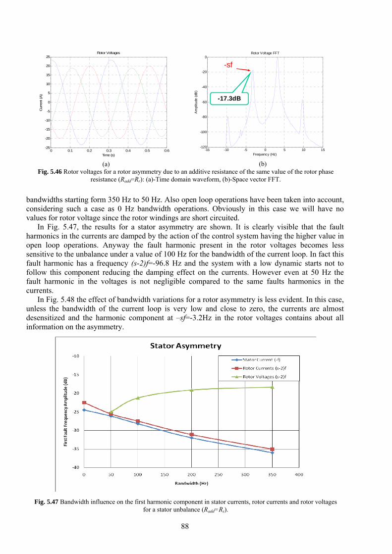
88
bandwidths starting form 350 Hz to 50 Hz. Also open loop operations have been taken into account, considering such a case as 0 Hz bandwidth operations. Obviously in this case we will have no values for rotor voltage since the rotor windings are short circuited.
In Fig. 5.47, the results for a stator asymmetry are shown. It is clearly visible that the fault harmonics in the currents are damped by the action of the control system having the higher value in open loop operations. Anyway the fault harmonic present in the rotor voltages becomes less sensitive to the unbalance under a value of 100 Hz for the bandwidth of the current loop. In fact this fault harmonic has a frequency (s-2)f=-96.8 Hz and the system with a low dynamic starts not to follow this component reducing the damping effect on the currents. However even at 50 Hz the fault harmonic in the voltages is not negligible compared to the same faults harmonics in the currents.
In Fig. 5.48 the effect of bandwidth variations for a rotor asymmetry is less evident. In this case, unless the bandwidth of the current loop is very low and close to zero, the currents are almost desensitized and the harmonic component at –sf=-3.2Hz in the rotor voltages contains about all information on the asymmetry.
0 0.1 0.2 0.3 0.4 0.5 0.6-25
-20
-15
-10
-5
0
5
10
15
20
25Rotor Voltages
Time (s)
Cur
rent
(A)
(a)
-15 -10 -5 0 5 10 15-120
-100
-80
-60
-40
-20
0Rotor Voltage FFT
Frequency (Hz)
Am
plitu
de (d
B)
-sf
-17.3dB
(b)
Fig. 5.46 Rotor voltages for a rotor asymmetry due to an additive resistance of the same value of the rotor phase resistance (Radd=Rr): (a)-Time domain waveform, (b)-Space vector FFT.
Fig. 5.47 Bandwidth influence on the first harmonic component in stator currents, rotor currents and rotor voltages for a stator unbalance (Radd=Rs).
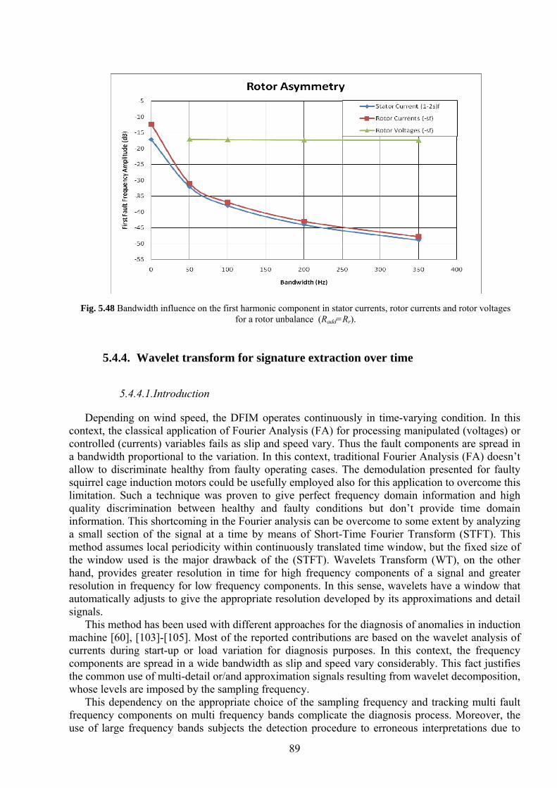
89
5.4.4. Wavelet transform for signature extraction over time
5.4.4.1.Introduction
Depending on wind speed, the DFIM operates continuously in time-varying condition. In this context, the classical application of Fourier Analysis (FA) for processing manipulated (voltages) or controlled (currents) variables fails as slip and speed vary. Thus the fault components are spread in a bandwidth proportional to the variation. In this context, traditional Fourier Analysis (FA) doesn’t allow to discriminate healthy from faulty operating cases. The demodulation presented for faulty squirrel cage induction motors could be usefully employed also for this application to overcome this limitation. Such a technique was proven to give perfect frequency domain information and high quality discrimination between healthy and faulty conditions but don’t provide time domain information. This shortcoming in the Fourier analysis can be overcome to some extent by analyzing a small section of the signal at a time by means of Short-Time Fourier Transform (STFT). This method assumes local periodicity within continuously translated time window, but the fixed size of the window used is the major drawback of the (STFT). Wavelets Transform (WT), on the other hand, provides greater resolution in time for high frequency components of a signal and greater resolution in frequency for low frequency components. In this sense, wavelets have a window that automatically adjusts to give the appropriate resolution developed by its approximations and detail signals.
This method has been used with different approaches for the diagnosis of anomalies in induction machine [60], [103]-[105]. Most of the reported contributions are based on the wavelet analysis of currents during start-up or load variation for diagnosis purposes. In this context, the frequency components are spread in a wide bandwidth as slip and speed vary considerably. This fact justifies the common use of multi-detail or/and approximation signals resulting from wavelet decomposition, whose levels are imposed by the sampling frequency.
This dependency on the appropriate choice of the sampling frequency and tracking multi fault frequency components on multi frequency bands complicate the diagnosis process. Moreover, the use of large frequency bands subjects the detection procedure to erroneous interpretations due to
Fig. 5.48 Bandwidth influence on the first harmonic component in stator currents, rotor currents and rotor voltages for a rotor unbalance (Radd=Rr).
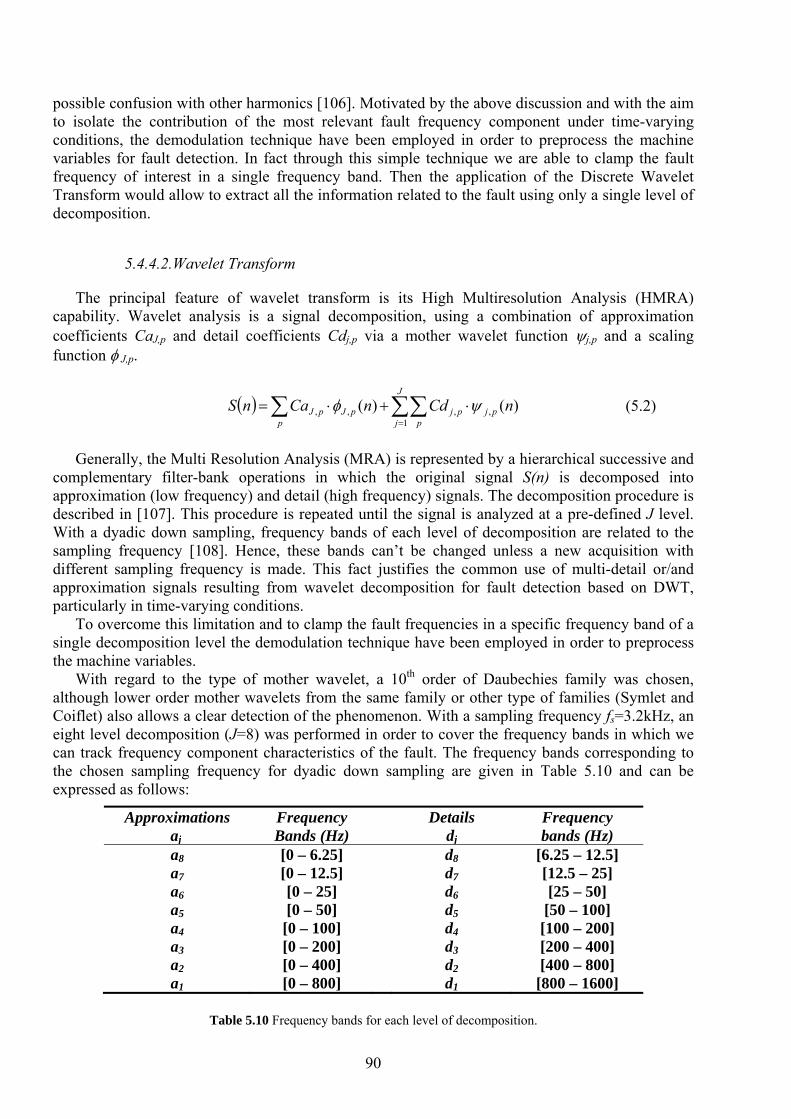
90
possible confusion with other harmonics [106]. Motivated by the above discussion and with the aim to isolate the contribution of the most relevant fault frequency component under time-varying conditions, the demodulation technique have been employed in order to preprocess the machine variables for fault detection. In fact through this simple technique we are able to clamp the fault frequency of interest in a single frequency band. Then the application of the Discrete Wavelet Transform would allow to extract all the information related to the fault using only a single level of decomposition.
5.4.4.2.Wavelet Transform
The principal feature of wavelet transform is its High Multiresolution Analysis (HMRA) capability. Wavelet analysis is a signal decomposition, using a combination of approximation coefficients CaJ,p and detail coefficients Cdj,p via a mother wavelet function ψj,p and a scaling function φ J,p.
( ) ∑∑∑=
⋅+⋅=J
j ppjpj
ppJpJ nCdnCanS
1,,,, )()( ψφ (5.2)
Generally, the Multi Resolution Analysis (MRA) is represented by a hierarchical successive and
complementary filter-bank operations in which the original signal S(n) is decomposed into approximation (low frequency) and detail (high frequency) signals. The decomposition procedure is described in [107]. This procedure is repeated until the signal is analyzed at a pre-defined J level. With a dyadic down sampling, frequency bands of each level of decomposition are related to the sampling frequency [108]. Hence, these bands can’t be changed unless a new acquisition with different sampling frequency is made. This fact justifies the common use of multi-detail or/and approximation signals resulting from wavelet decomposition for fault detection based on DWT, particularly in time-varying conditions.
To overcome this limitation and to clamp the fault frequencies in a specific frequency band of a single decomposition level the demodulation technique have been employed in order to preprocess the machine variables.
With regard to the type of mother wavelet, a 10th order of Daubechies family was chosen, although lower order mother wavelets from the same family or other type of families (Symlet and Coiflet) also allows a clear detection of the phenomenon. With a sampling frequency fs=3.2kHz, an eight level decomposition (J=8) was performed in order to cover the frequency bands in which we can track frequency component characteristics of the fault. The frequency bands corresponding to the chosen sampling frequency for dyadic down sampling are given in Table 5.10 and can be expressed as follows:
Approximations aj
Frequency Bands (Hz)
Details dj
Frequency bands (Hz)
a8 [0 – 6.25] d8 [6.25 – 12.5] a7 [0 – 12.5] d7 [12.5 – 25] a6 [0 – 25] d6 [25 – 50] a5 [0 – 50] d5 [50 – 100] a4 [0 – 100] d4 [100 – 200] a3 [0 – 200] d3 [200 – 400] a2 [0 – 400] d2 [400 – 800] a1 [0 – 800] d1 [800 – 1600]
Table 5.10 Frequency bands for each level of decomposition.
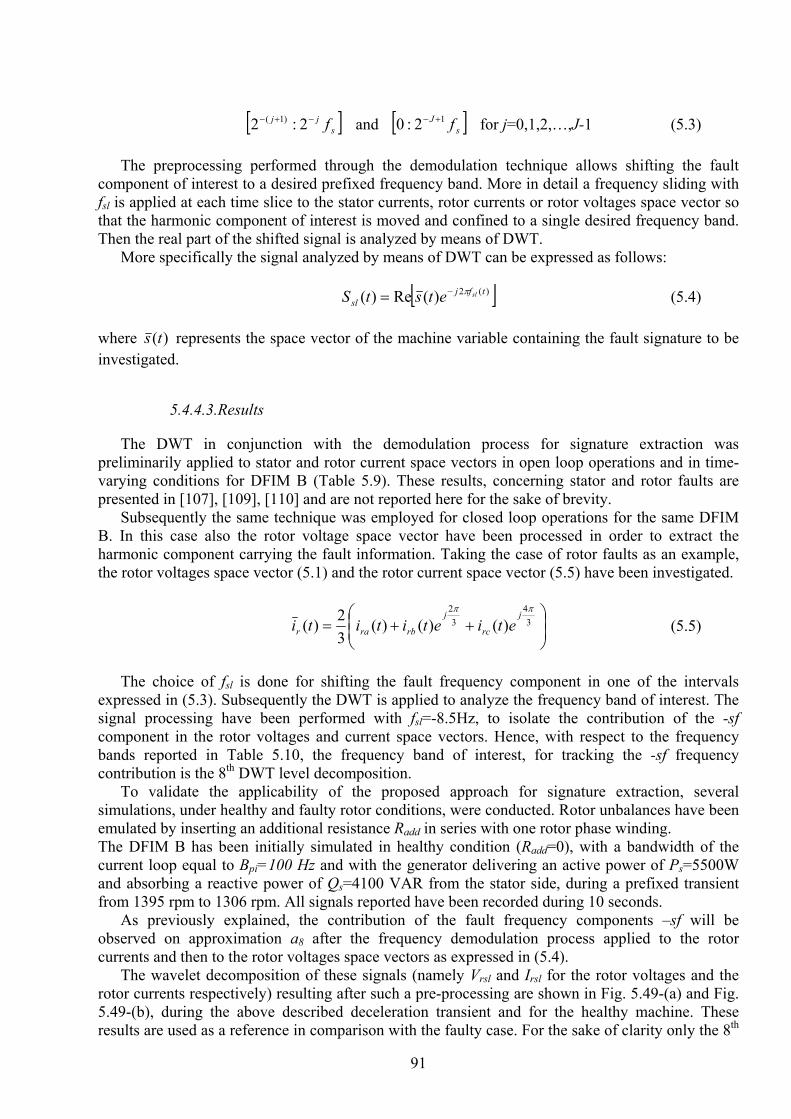
91
[ ]s
jj f−+− 2:2 )1( and [ ]sJ f12:0 +− for j=0,1,2,…,J-1 (5.3)
The preprocessing performed through the demodulation technique allows shifting the fault
component of interest to a desired prefixed frequency band. More in detail a frequency sliding with fsl is applied at each time slice to the stator currents, rotor currents or rotor voltages space vector so that the harmonic component of interest is moved and confined to a single desired frequency band. Then the real part of the shifted signal is analyzed by means of DWT.
More specifically the signal analyzed by means of DWT can be expressed as follows: [ ])(2)(Re)( tfj
slsletstS π−= (5.4)
where )(ts represents the space vector of the machine variable containing the fault signature to be investigated.
5.4.4.3.Results
The DWT in conjunction with the demodulation process for signature extraction was preliminarily applied to stator and rotor current space vectors in open loop operations and in time-varying conditions for DFIM B (Table 5.9). These results, concerning stator and rotor faults are presented in [107], [109], [110] and are not reported here for the sake of brevity.
Subsequently the same technique was employed for closed loop operations for the same DFIM B. In this case also the rotor voltage space vector have been processed in order to extract the harmonic component carrying the fault information. Taking the case of rotor faults as an example, the rotor voltages space vector (5.1) and the rotor current space vector (5.5) have been investigated.
⎟⎟⎠
⎞⎜⎜⎝
⎛++= 3
43
2
)()()(32)(
ππ j
rc
j
rbrar etietititi (5.5)
The choice of fsl is done for shifting the fault frequency component in one of the intervals
expressed in (5.3). Subsequently the DWT is applied to analyze the frequency band of interest. The signal processing have been performed with fsl=-8.5Hz, to isolate the contribution of the -sf component in the rotor voltages and current space vectors. Hence, with respect to the frequency bands reported in Table 5.10, the frequency band of interest, for tracking the -sf frequency contribution is the 8th DWT level decomposition.
To validate the applicability of the proposed approach for signature extraction, several simulations, under healthy and faulty rotor conditions, were conducted. Rotor unbalances have been emulated by inserting an additional resistance Radd in series with one rotor phase winding. The DFIM B has been initially simulated in healthy condition (Radd=0), with a bandwidth of the current loop equal to Bpi=100 Hz and with the generator delivering an active power of Ps=5500W and absorbing a reactive power of Qs=4100 VAR from the stator side, during a prefixed transient from 1395 rpm to 1306 rpm. All signals reported have been recorded during 10 seconds.
As previously explained, the contribution of the fault frequency components –sf will be observed on approximation a8 after the frequency demodulation process applied to the rotor currents and then to the rotor voltages space vectors as expressed in (5.4).
The wavelet decomposition of these signals (namely Vrsl and Irsl for the rotor voltages and the rotor currents respectively) resulting after such a pre-processing are shown in Fig. 5.49-(a) and Fig. 5.49-(b), during the above described deceleration transient and for the healthy machine. These results are used as a reference in comparison with the faulty case. For the sake of clarity only the 8th
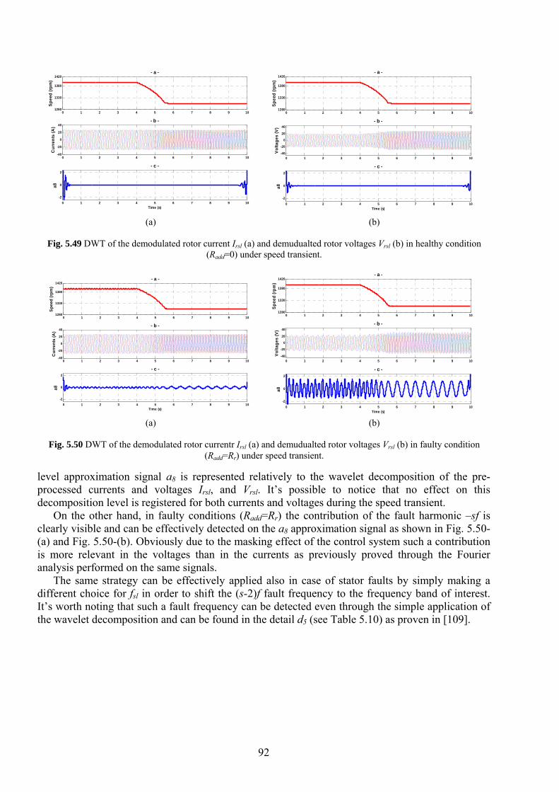
92
level approximation signal a8 is represented relatively to the wavelet decomposition of the pre-processed currents and voltages Irsl, and Vrsl. It’s possible to notice that no effect on this decomposition level is registered for both currents and voltages during the speed transient.
On the other hand, in faulty conditions (Radd=Rr) the contribution of the fault harmonic –sf is clearly visible and can be effectively detected on the a8 approximation signal as shown in Fig. 5.50-(a) and Fig. 5.50-(b). Obviously due to the masking effect of the control system such a contribution is more relevant in the voltages than in the currents as previously proved through the Fourier analysis performed on the same signals.
The same strategy can be effectively applied also in case of stator faults by simply making a different choice for fsl in order to shift the (s-2)f fault frequency to the frequency band of interest. It’s worth noting that such a fault frequency can be detected even through the simple application of the wavelet decomposition and can be found in the detail d5 (see Table 5.10) as proven in [109].
0 1 2 3 4 5 6 7 8 9 101280
1330
1380
1420- a -
Spee
d (rp
m)
0 1 2 3 4 5 6 7 8 9 10-2
0
2
- c -
Time (s)
a8
0 1 2 3 4 5 6 7 8 9 10-40
-20
0
20
40- b -
Cur
rent
s (A
)
(a)
0 1 2 3 4 5 6 7 8 9 101280
1330
1380
1420- a -
Spee
d (rp
m)
0 1 2 3 4 5 6 7 8 9 10-2
0
2
- c -
Time (s)
a8
0 1 2 3 4 5 6 7 8 9 10-40
-20
0
20
40- b -
Volta
ges
(V)
(b)
Fig. 5.49 DWT of the demodulated rotor current Irsl (a) and demudualted rotor voltages Vrsl (b) in healthy condition (Radd=0) under speed transient.
0 1 2 3 4 5 6 7 8 9 101280
1330
1380
1420- a -
Spe
ed (r
pm)
0 1 2 3 4 5 6 7 8 9 10-2
0
2
- c -
Time (s)
a8
0 1 2 3 4 5 6 7 8 9 10-40
-20
0
20
40- b -
Cur
rent
s (A
)
(a)
0 1 2 3 4 5 6 7 8 9 101280
1330
1380
1420- a -
Spee
d (rp
m)
0 1 2 3 4 5 6 7 8 9 10-2
0
2
- c -
Time (s)
a8
0 1 2 3 4 5 6 7 8 9 10-40
-20
0
20
40- b -
Volta
ges
(V)
(b)
Fig. 5.50 DWT of the demodulated rotor currentr Irsl (a) and demudualted rotor voltages Vrsl (b) in faulty condition (Radd=Rr) under speed transient.
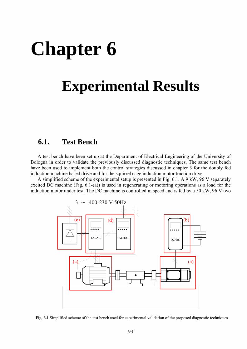
93
Chapter 6
Experimental Results
6.1. Test Bench
A test bench have been set up at the Department of Electrical Engineering of the University of Bologna in order to validate the previously discussed diagnostic techniques. The same test bench have been used to implement both the control strategies discussed in chapter 3 for the doubly fed induction machine based drive and for the squirrel cage induction motor traction drive.
A simplified scheme of the experimental setup is presented in Fig. 6.1. A 9 kW, 96 V separately excited DC machine (Fig. 6.1-(a)) is used in regenerating or motoring operations as a load for the induction motor under test. The DC machine is controlled in speed and is fed by a 50 kW, 96 V two
AC/DC DC/DC
(c) (a)
(b)(d)
DC/AC
3 ~ 400-230 V 50Hz
(e)
Fig. 6.1 Simplified scheme of the test bench used for experimental validation of the proposed diagnostic techniques
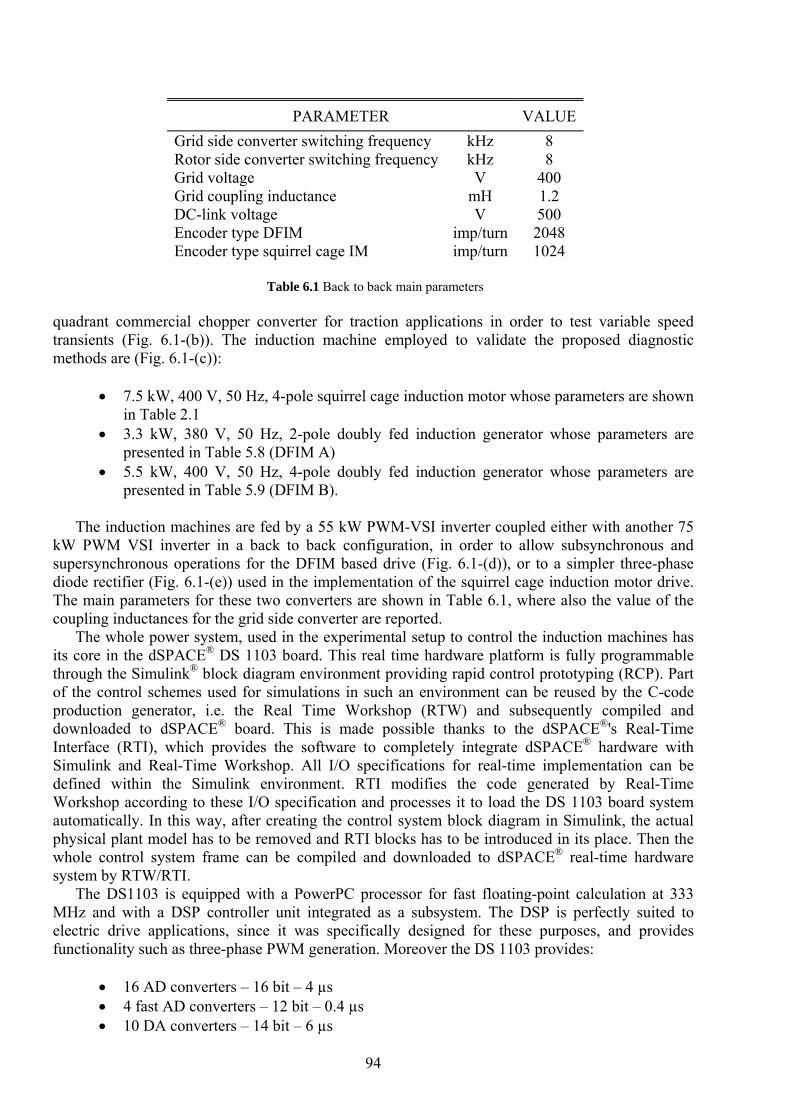
94
quadrant commercial chopper converter for traction applications in order to test variable speed transients (Fig. 6.1-(b)). The induction machine employed to validate the proposed diagnostic methods are (Fig. 6.1-(c)):
• 7.5 kW, 400 V, 50 Hz, 4-pole squirrel cage induction motor whose parameters are shown
in Table 2.1 • 3.3 kW, 380 V, 50 Hz, 2-pole doubly fed induction generator whose parameters are
presented in Table 5.8 (DFIM A) • 5.5 kW, 400 V, 50 Hz, 4-pole doubly fed induction generator whose parameters are
presented in Table 5.9 (DFIM B). The induction machines are fed by a 55 kW PWM-VSI inverter coupled either with another 75
kW PWM VSI inverter in a back to back configuration, in order to allow subsynchronous and supersynchronous operations for the DFIM based drive (Fig. 6.1-(d)), or to a simpler three-phase diode rectifier (Fig. 6.1-(e)) used in the implementation of the squirrel cage induction motor drive. The main parameters for these two converters are shown in Table 6.1, where also the value of the coupling inductances for the grid side converter are reported.
The whole power system, used in the experimental setup to control the induction machines has its core in the dSPACE® DS 1103 board. This real time hardware platform is fully programmable through the Simulink® block diagram environment providing rapid control prototyping (RCP). Part of the control schemes used for simulations in such an environment can be reused by the C-code production generator, i.e. the Real Time Workshop (RTW) and subsequently compiled and downloaded to dSPACE® board. This is made possible thanks to the dSPACE®'s Real-Time Interface (RTI), which provides the software to completely integrate dSPACE® hardware with Simulink and Real-Time Workshop. All I/O specifications for real-time implementation can be defined within the Simulink environment. RTI modifies the code generated by Real-Time Workshop according to these I/O specification and processes it to load the DS 1103 board system automatically. In this way, after creating the control system block diagram in Simulink, the actual physical plant model has to be removed and RTI blocks has to be introduced in its place. Then the whole control system frame can be compiled and downloaded to dSPACE® real-time hardware system by RTW/RTI.
The DS1103 is equipped with a PowerPC processor for fast floating-point calculation at 333 MHz and with a DSP controller unit integrated as a subsystem. The DSP is perfectly suited to electric drive applications, since it was specifically designed for these purposes, and provides functionality such as three-phase PWM generation. Moreover the DS 1103 provides:
• 16 AD converters – 16 bit – 4 µs • 4 fast AD converters – 12 bit – 0.4 µs • 10 DA converters – 14 bit – 6 µs
PARAMETER VALUE Grid side converter switching frequency kHz 8 Rotor side converter switching frequency kHz 8 Grid voltage V 400 Grid coupling inductance mH 1.2 DC-link voltage V 500 Encoder type DFIM imp/turn 2048 Encoder type squirrel cage IM imp/turn 1024
Table 6.1 Back to back main parameters
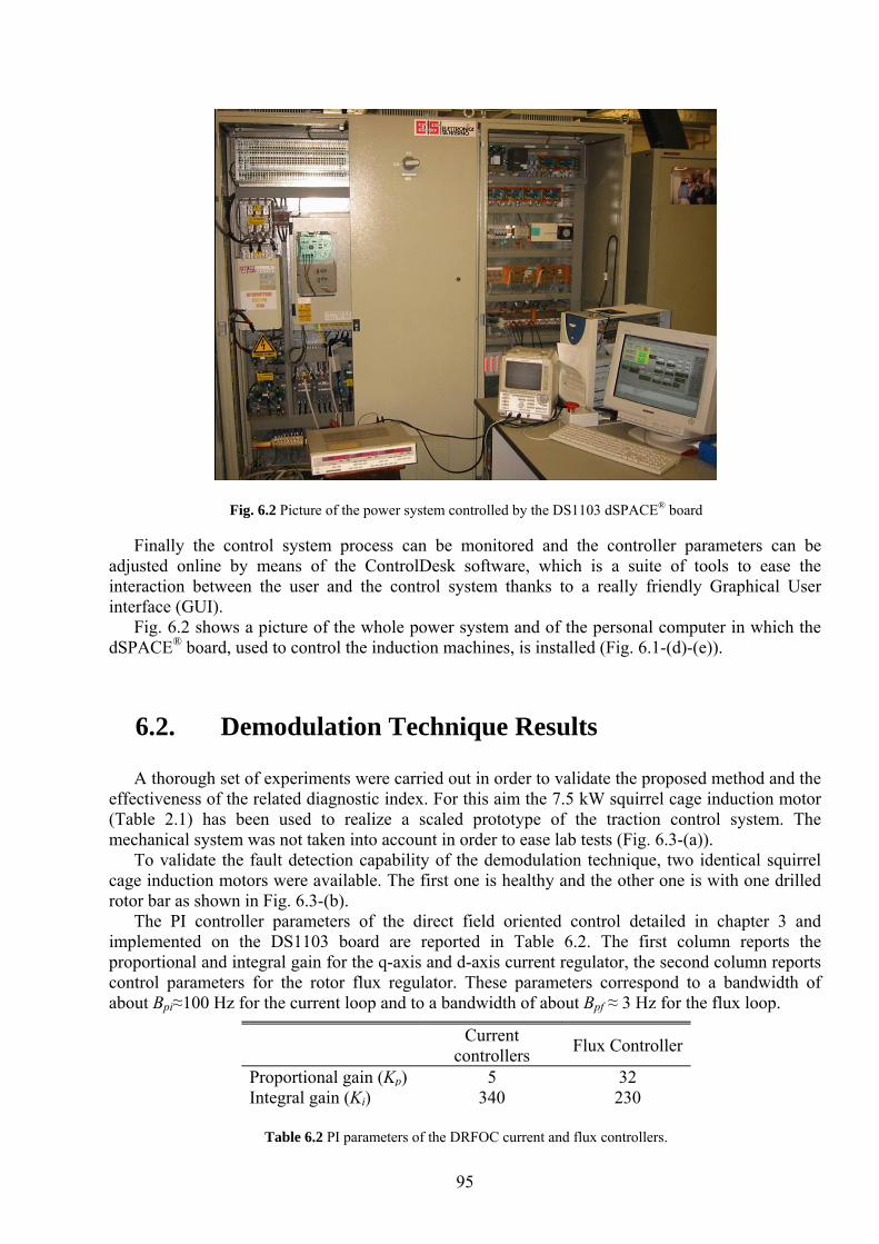
95
Finally the control system process can be monitored and the controller parameters can be adjusted online by means of the ControlDesk software, which is a suite of tools to ease the interaction between the user and the control system thanks to a really friendly Graphical User interface (GUI).
Fig. 6.2 shows a picture of the whole power system and of the personal computer in which the dSPACE® board, used to control the induction machines, is installed (Fig. 6.1-(d)-(e)).
6.2. Demodulation Technique Results
A thorough set of experiments were carried out in order to validate the proposed method and the effectiveness of the related diagnostic index. For this aim the 7.5 kW squirrel cage induction motor (Table 2.1) has been used to realize a scaled prototype of the traction control system. The mechanical system was not taken into account in order to ease lab tests (Fig. 6.3-(a)).
To validate the fault detection capability of the demodulation technique, two identical squirrel cage induction motors were available. The first one is healthy and the other one is with one drilled rotor bar as shown in Fig. 6.3-(b).
The PI controller parameters of the direct field oriented control detailed in chapter 3 and implemented on the DS1103 board are reported in Table 6.2. The first column reports the proportional and integral gain for the q-axis and d-axis current regulator, the second column reports control parameters for the rotor flux regulator. These parameters correspond to a bandwidth of about Bpi≈100 Hz for the current loop and to a bandwidth of about Bpf ≈ 3 Hz for the flux loop.
Fig. 6.2 Picture of the power system controlled by the DS1103 dSPACE® board
Current controllers Flux Controller
Proportional gain (Kp) 5 32 Integral gain (Ki) 340 230
Table 6.2 PI parameters of the DRFOC current and flux controllers.
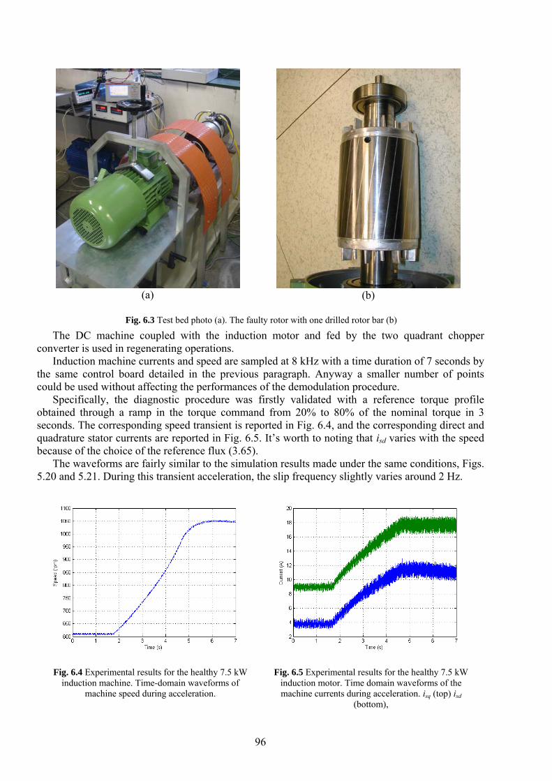
96
The DC machine coupled with the induction motor and fed by the two quadrant chopper converter is used in regenerating operations.
Induction machine currents and speed are sampled at 8 kHz with a time duration of 7 seconds by the same control board detailed in the previous paragraph. Anyway a smaller number of points could be used without affecting the performances of the demodulation procedure.
Specifically, the diagnostic procedure was firstly validated with a reference torque profile obtained through a ramp in the torque command from 20% to 80% of the nominal torque in 3 seconds. The corresponding speed transient is reported in Fig. 6.4, and the corresponding direct and quadrature stator currents are reported in Fig. 6.5. It’s worth to noting that isd varies with the speed because of the choice of the reference flux (3.65).
The waveforms are fairly similar to the simulation results made under the same conditions, Figs. 5.20 and 5.21. During this transient acceleration, the slip frequency slightly varies around 2 Hz.
(a)
(b)
Fig. 6.3 Test bed photo (a). The faulty rotor with one drilled rotor bar (b)
Fig. 6.4 Experimental results for the healthy 7.5 kW induction machine. Time-domain waveforms of
machine speed during acceleration.
Fig. 6.5 Experimental results for the healthy 7.5 kW induction motor. Time domain waveforms of the machine currents during acceleration. isq (top) isd
(bottom),
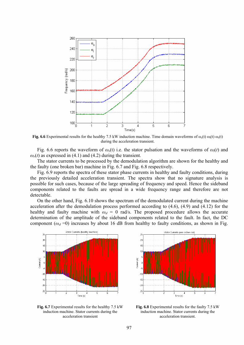
97
Fig. 6.6 reports the waveform of ωs(t) i.e. the stator pulsation and the waveforms of ωl(t) and ωr(t) as expressed in (4.1) and (4.2) during the transient.
The stator currents to be processed by the demodulation algorithm are shown for the healthy and the faulty (one broken bar) machine in Fig. 6.7 and Fig. 6.8 respectively.
Fig. 6.9 reports the spectra of these stator phase currents in healthy and faulty conditions, during the previously detailed acceleration transient. The spectra show that no signature analysis is possible for such cases, because of the large spreading of frequency and speed. Hence the sideband components related to the faults are spread in a wide frequency range and therefore are not detectable.
On the other hand, Fig. 6.10 shows the spectrum of the demodulated current during the machine acceleration after the demodulation process performed according to (4.6), (4.9) and (4.12) for the healthy and faulty machine with ωd = 0 rad/s. The proposed procedure allows the accurate determination of the amplitude of the sideband components related to the fault. In fact, the DC component (ωd =0) increases by about 16 dB from healthy to faulty conditions, as shown in Fig.
Fig. 6.6 Experimental results for the healthy 7.5 kW induction machine. Time domain waveforms of ωs(t) ωl(t) ωr(t)
during the acceleration transient.
Fig. 6.7 Experimental results for the healthy 7.5 kW induction machine. Stator currents during the
acceleration transient
Fig. 6.8 Experimental results for the faulty 7.5 kW
induction machine. Stator currents during the acceleration transient.
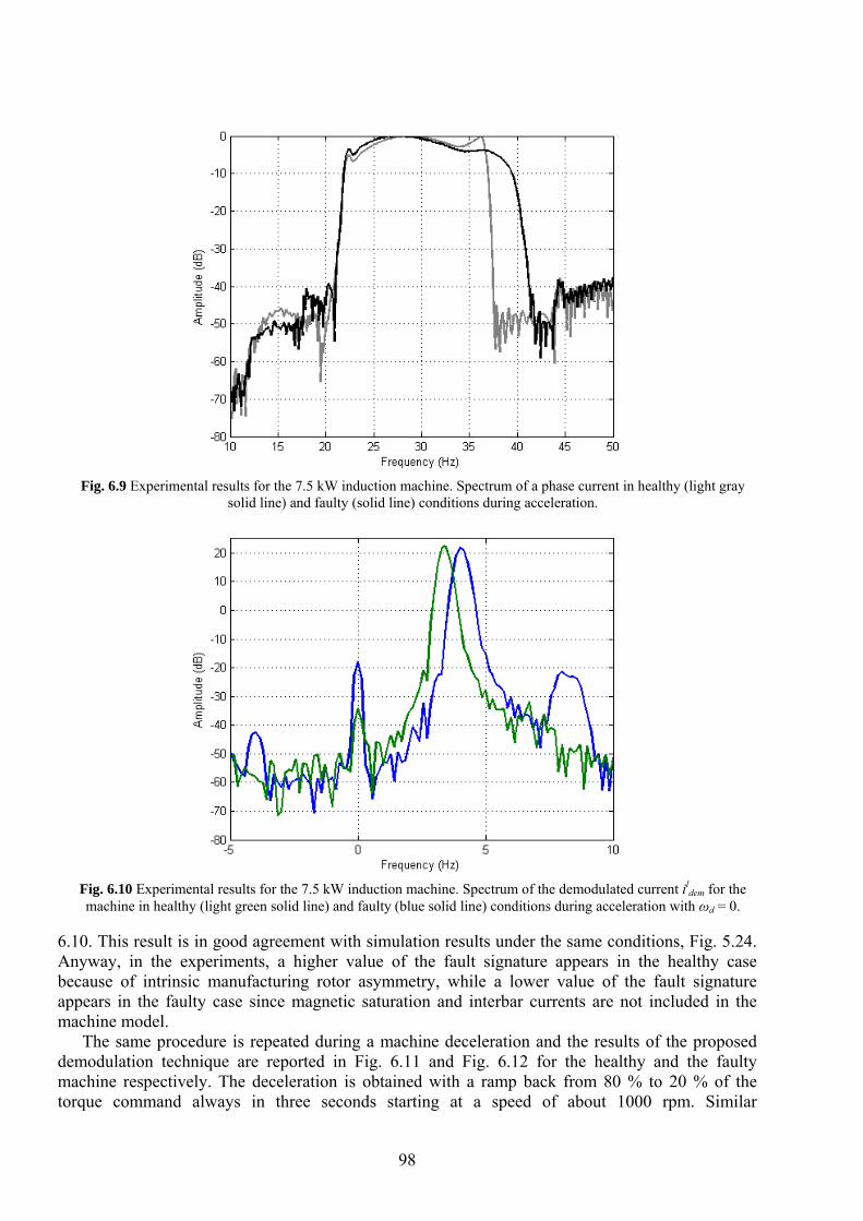
98
6.10. This result is in good agreement with simulation results under the same conditions, Fig. 5.24. Anyway, in the experiments, a higher value of the fault signature appears in the healthy case because of intrinsic manufacturing rotor asymmetry, while a lower value of the fault signature appears in the faulty case since magnetic saturation and interbar currents are not included in the machine model.
The same procedure is repeated during a machine deceleration and the results of the proposed demodulation technique are reported in Fig. 6.11 and Fig. 6.12 for the healthy and the faulty machine respectively. The deceleration is obtained with a ramp back from 80 % to 20 % of the torque command always in three seconds starting at a speed of about 1000 rpm. Similar
Fig. 6.9 Experimental results for the 7.5 kW induction machine. Spectrum of a phase current in healthy (light gray
solid line) and faulty (solid line) conditions during acceleration.
Fig. 6.10 Experimental results for the 7.5 kW induction machine. Spectrum of the demodulated current il
dem for the machine in healthy (light green solid line) and faulty (blue solid line) conditions during acceleration with ωd = 0.
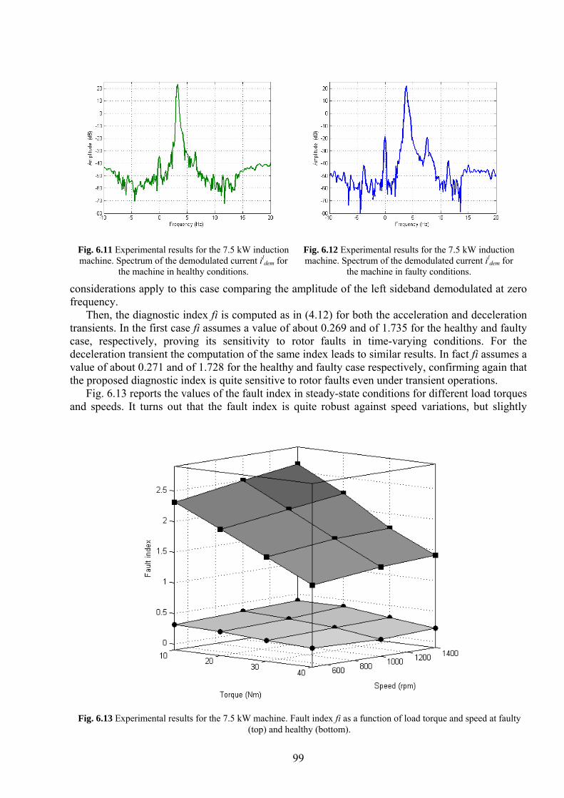
99
considerations apply to this case comparing the amplitude of the left sideband demodulated at zero frequency.
Then, the diagnostic index fi is computed as in (4.12) for both the acceleration and deceleration transients. In the first case fi assumes a value of about 0.269 and of 1.735 for the healthy and faulty case, respectively, proving its sensitivity to rotor faults in time-varying conditions. For the deceleration transient the computation of the same index leads to similar results. In fact fi assumes a value of about 0.271 and of 1.728 for the healthy and faulty case respectively, confirming again that the proposed diagnostic index is quite sensitive to rotor faults even under transient operations.
Fig. 6.13 reports the values of the fault index in steady-state conditions for different load torques and speeds. It turns out that the fault index is quite robust against speed variations, but slightly
Fig. 6.11 Experimental results for the 7.5 kW induction machine. Spectrum of the demodulated current il
dem for the machine in healthy conditions.
Fig. 6.12 Experimental results for the 7.5 kW induction machine. Spectrum of the demodulated current il
dem for the machine in faulty conditions.
Fig. 6.13 Experimental results for the 7.5 kW machine. Fault index fi as a function of load torque and speed at faulty
(top) and healthy (bottom).
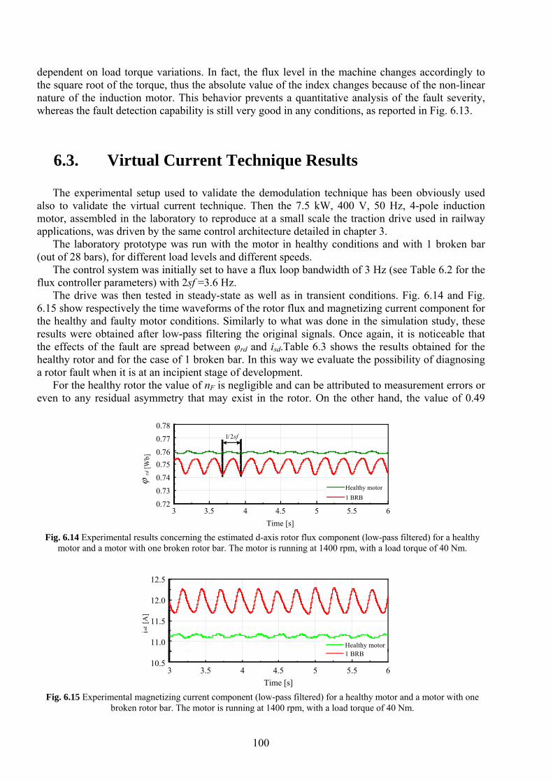
100
dependent on load torque variations. In fact, the flux level in the machine changes accordingly to the square root of the torque, thus the absolute value of the index changes because of the non-linear nature of the induction motor. This behavior prevents a quantitative analysis of the fault severity, whereas the fault detection capability is still very good in any conditions, as reported in Fig. 6.13.
6.3. Virtual Current Technique Results
The experimental setup used to validate the demodulation technique has been obviously used also to validate the virtual current technique. Then the 7.5 kW, 400 V, 50 Hz, 4-pole induction motor, assembled in the laboratory to reproduce at a small scale the traction drive used in railway applications, was driven by the same control architecture detailed in chapter 3.
The laboratory prototype was run with the motor in healthy conditions and with 1 broken bar (out of 28 bars), for different load levels and different speeds.
The control system was initially set to have a flux loop bandwidth of 3 Hz (see Table 6.2 for the flux controller parameters) with 2sf =3.6 Hz.
The drive was then tested in steady-state as well as in transient conditions. Fig. 6.14 and Fig. 6.15 show respectively the time waveforms of the rotor flux and magnetizing current component for the healthy and faulty motor conditions. Similarly to what was done in the simulation study, these results were obtained after low-pass filtering the original signals. Once again, it is noticeable that the effects of the fault are spread between φrd and isd.Table 6.3 shows the results obtained for the healthy rotor and for the case of 1 broken bar. In this way we evaluate the possibility of diagnosing a rotor fault when it is at an incipient stage of development.
For the healthy rotor the value of nF is negligible and can be attributed to measurement errors or even to any residual asymmetry that may exist in the rotor. On the other hand, the value of 0.49
1/2sf
3 3.5 4 4.5 5 5.5 6Time [s]
0.72
0.73
0.74
0.750.760.77
0.78
Healthy motor1 BRB
ϕ rd
[Wb]
Fig. 6.14 Experimental results concerning the estimated d-axis rotor flux component (low-pass filtered) for a healthy
motor and a motor with one broken rotor bar. The motor is running at 1400 rpm, with a load torque of 40 Nm.
3 3.5 4 4.5 5 5.5 6Time [s]
10.5
11.0
11.5
12.0
12.5
isd [A
]
Healthy motor1 BRB
Fig. 6.15 Experimental magnetizing current component (low-pass filtered) for a healthy motor and a motor with one
broken rotor bar. The motor is running at 1400 rpm, with a load torque of 40 Nm.
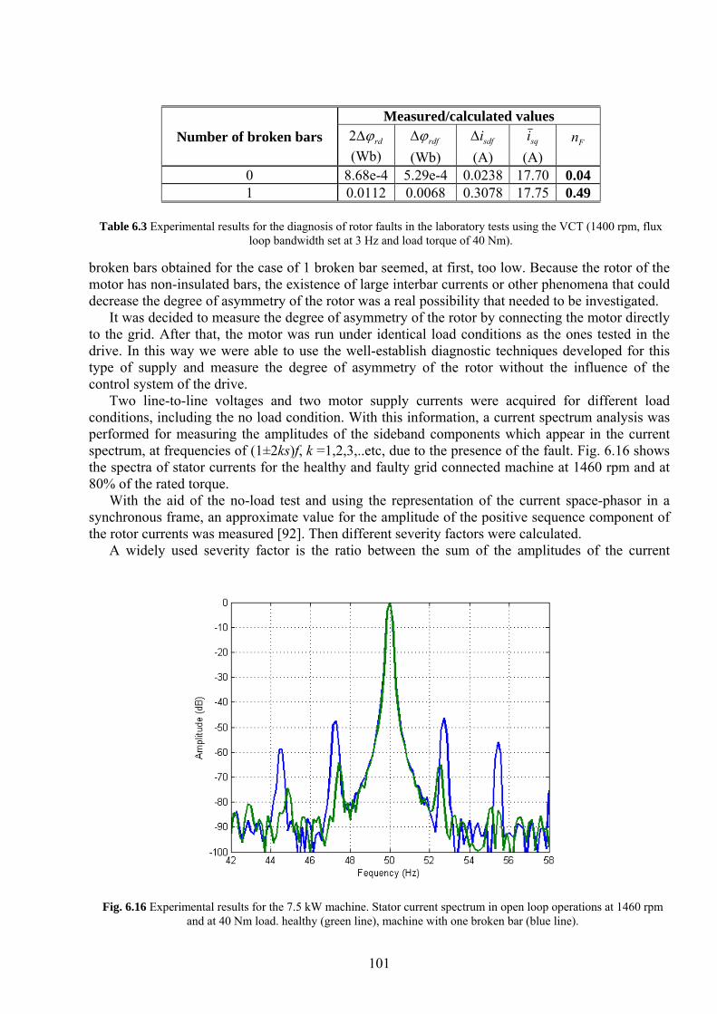
101
broken bars obtained for the case of 1 broken bar seemed, at first, too low. Because the rotor of the motor has non-insulated bars, the existence of large interbar currents or other phenomena that could decrease the degree of asymmetry of the rotor was a real possibility that needed to be investigated.
It was decided to measure the degree of asymmetry of the rotor by connecting the motor directly to the grid. After that, the motor was run under identical load conditions as the ones tested in the drive. In this way we were able to use the well-establish diagnostic techniques developed for this type of supply and measure the degree of asymmetry of the rotor without the influence of the control system of the drive.
Two line-to-line voltages and two motor supply currents were acquired for different load conditions, including the no load condition. With this information, a current spectrum analysis was performed for measuring the amplitudes of the sideband components which appear in the current spectrum, at frequencies of (1±2ks)f, k =1,2,3,..etc, due to the presence of the fault. Fig. 6.16 shows the spectra of stator currents for the healthy and faulty grid connected machine at 1460 rpm and at 80% of the rated torque.
With the aid of the no-load test and using the representation of the current space-phasor in a synchronous frame, an approximate value for the amplitude of the positive sequence component of the rotor currents was measured [92]. Then different severity factors were calculated.
A widely used severity factor is the ratio between the sum of the amplitudes of the current
Number of broken bars Measured/calculated values
rdϕΔ2 (Wb)
rdfϕΔ (Wb)
sdfiΔ (A)
sqi (A)
Fn
0 8.68e-4 5.29e-4 0.0238 17.70 0.04 1 0.0112 0.0068 0.3078 17.75 0.49
Table 6.3 Experimental results for the diagnosis of rotor faults in the laboratory tests using the VCT (1400 rpm, flux
loop bandwidth set at 3 Hz and load torque of 40 Nm).
Fig. 6.16 Experimental results for the 7.5 kW machine. Stator current spectrum in open loop operations at 1460 rpm and at 40 Nm load. healthy (green line), machine with one broken bar (blue line).
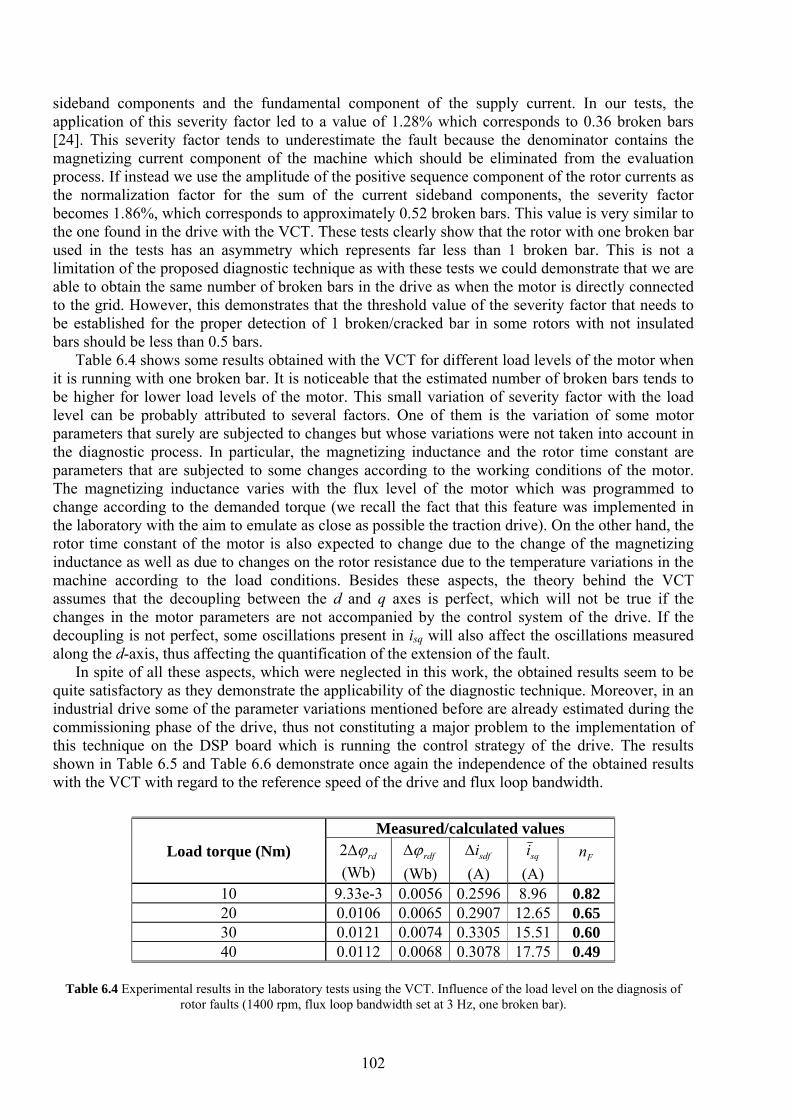
102
sideband components and the fundamental component of the supply current. In our tests, the application of this severity factor led to a value of 1.28% which corresponds to 0.36 broken bars [24]. This severity factor tends to underestimate the fault because the denominator contains the magnetizing current component of the machine which should be eliminated from the evaluation process. If instead we use the amplitude of the positive sequence component of the rotor currents as the normalization factor for the sum of the current sideband components, the severity factor becomes 1.86%, which corresponds to approximately 0.52 broken bars. This value is very similar to the one found in the drive with the VCT. These tests clearly show that the rotor with one broken bar used in the tests has an asymmetry which represents far less than 1 broken bar. This is not a limitation of the proposed diagnostic technique as with these tests we could demonstrate that we are able to obtain the same number of broken bars in the drive as when the motor is directly connected to the grid. However, this demonstrates that the threshold value of the severity factor that needs to be established for the proper detection of 1 broken/cracked bar in some rotors with not insulated bars should be less than 0.5 bars.
Table 6.4 shows some results obtained with the VCT for different load levels of the motor when it is running with one broken bar. It is noticeable that the estimated number of broken bars tends to be higher for lower load levels of the motor. This small variation of severity factor with the load level can be probably attributed to several factors. One of them is the variation of some motor parameters that surely are subjected to changes but whose variations were not taken into account in the diagnostic process. In particular, the magnetizing inductance and the rotor time constant are parameters that are subjected to some changes according to the working conditions of the motor. The magnetizing inductance varies with the flux level of the motor which was programmed to change according to the demanded torque (we recall the fact that this feature was implemented in the laboratory with the aim to emulate as close as possible the traction drive). On the other hand, the rotor time constant of the motor is also expected to change due to the change of the magnetizing inductance as well as due to changes on the rotor resistance due to the temperature variations in the machine according to the load conditions. Besides these aspects, the theory behind the VCT assumes that the decoupling between the d and q axes is perfect, which will not be true if the changes in the motor parameters are not accompanied by the control system of the drive. If the decoupling is not perfect, some oscillations present in isq will also affect the oscillations measured along the d-axis, thus affecting the quantification of the extension of the fault.
In spite of all these aspects, which were neglected in this work, the obtained results seem to be quite satisfactory as they demonstrate the applicability of the diagnostic technique. Moreover, in an industrial drive some of the parameter variations mentioned before are already estimated during the commissioning phase of the drive, thus not constituting a major problem to the implementation of this technique on the DSP board which is running the control strategy of the drive. The results shown in Table 6.5 and Table 6.6 demonstrate once again the independence of the obtained results with the VCT with regard to the reference speed of the drive and flux loop bandwidth.
Load torque (Nm) Measured/calculated values
rdϕΔ2 (Wb)
rdfϕΔ (Wb)
sdfiΔ (A)
sqi (A)
Fn
10 9.33e-3 0.0056 0.2596 8.96 0.82 20 0.0106 0.0065 0.2907 12.65 0.65 30 0.0121 0.0074 0.3305 15.51 0.60 40 0.0112 0.0068 0.3078 17.75 0.49
Table 6.4 Experimental results in the laboratory tests using the VCT. Influence of the load level on the diagnosis of
rotor faults (1400 rpm, flux loop bandwidth set at 3 Hz, one broken bar).
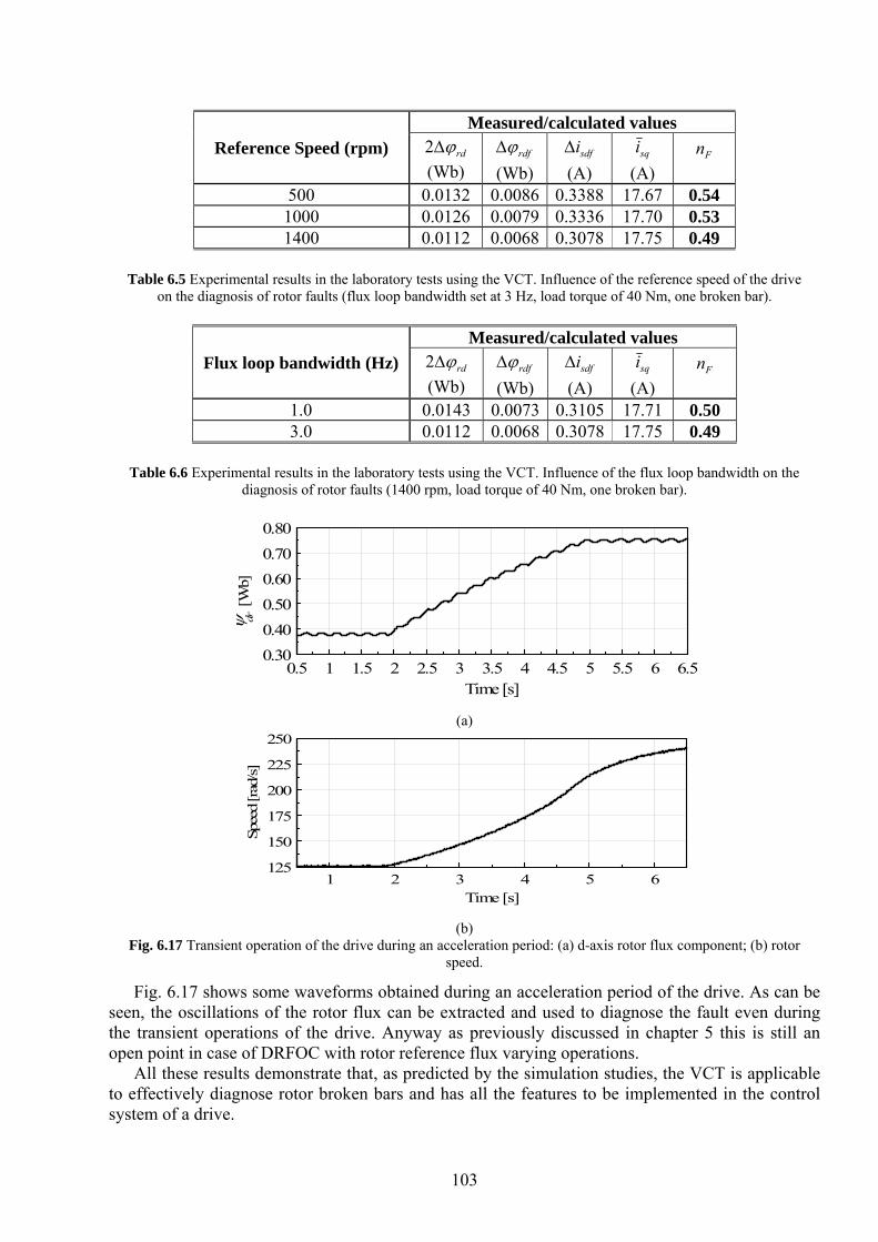
103
Fig. 6.17 shows some waveforms obtained during an acceleration period of the drive. As can be seen, the oscillations of the rotor flux can be extracted and used to diagnose the fault even during the transient operations of the drive. Anyway as previously discussed in chapter 5 this is still an open point in case of DRFOC with rotor reference flux varying operations.
All these results demonstrate that, as predicted by the simulation studies, the VCT is applicable to effectively diagnose rotor broken bars and has all the features to be implemented in the control system of a drive.
Reference Speed (rpm) Measured/calculated values
rdϕΔ2 (Wb)
rdfϕΔ (Wb)
sdfiΔ (A)
sqi (A)
Fn
500 0.0132 0.0086 0.3388 17.67 0.54 1000 0.0126 0.0079 0.3336 17.70 0.53 1400 0.0112 0.0068 0.3078 17.75 0.49
Table 6.5 Experimental results in the laboratory tests using the VCT. Influence of the reference speed of the drive
on the diagnosis of rotor faults (flux loop bandwidth set at 3 Hz, load torque of 40 Nm, one broken bar).
Flux loop bandwidth (Hz) Measured/calculated values
rdϕΔ2 (Wb)
rdfϕΔ (Wb)
sdfiΔ (A)
sqi (A)
Fn
1.0 0.0143 0.0073 0.3105 17.71 0.50 3.0 0.0112 0.0068 0.3078 17.75 0.49
Table 6.6 Experimental results in the laboratory tests using the VCT. Influence of the flux loop bandwidth on the
diagnosis of rotor faults (1400 rpm, load torque of 40 Nm, one broken bar).
0.5 1 1.5 2 2.5 3 3.5 4 4.5 5 5.5 6 6.5Time [s]
0.300.400.500.600.700.80
ψ dr[W
b]
(a)
1 2 3 4 5 6Time [s]
125
150
175
200
225
250
Spee
d [ra d
/s]
(b) Fig. 6.17 Transient operation of the drive during an acceleration period: (a) d-axis rotor flux component; (b) rotor
speed.
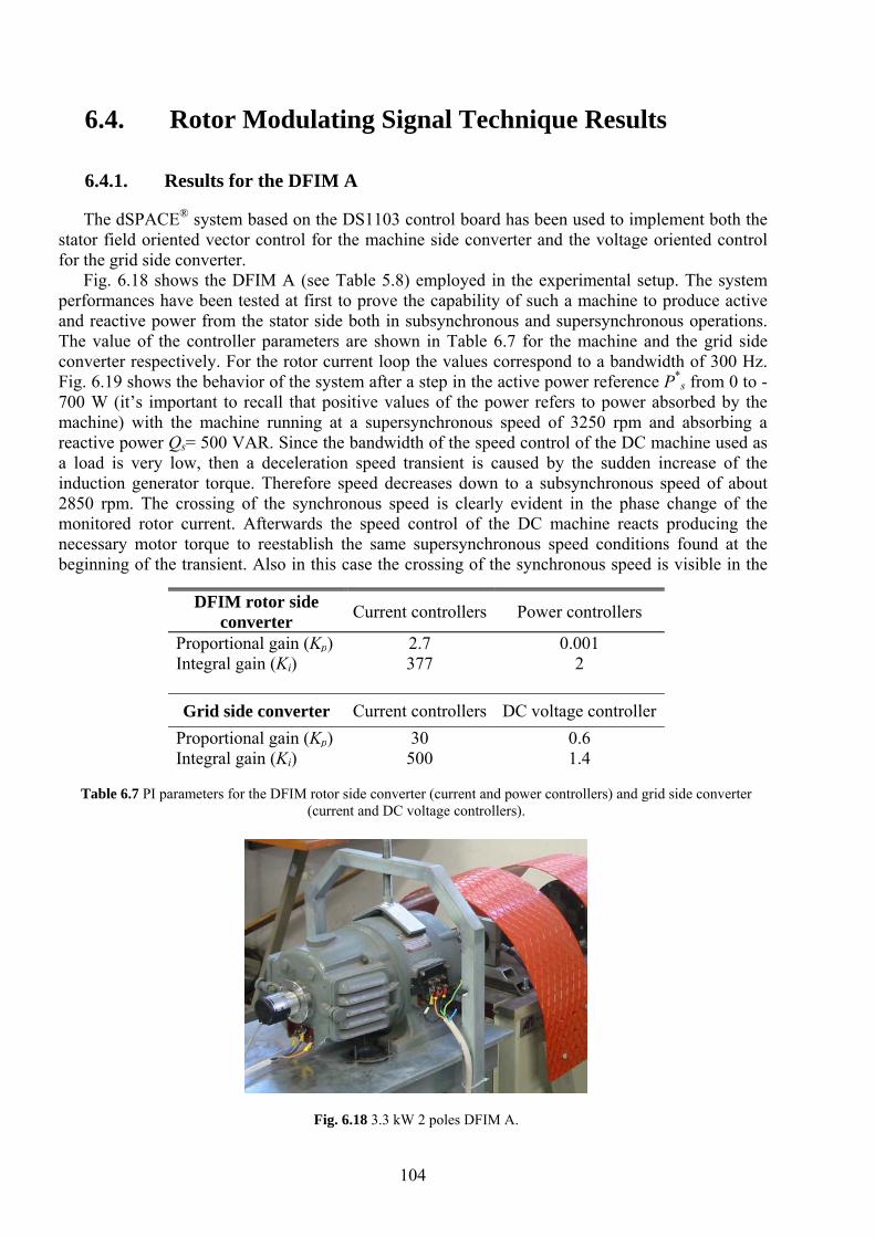
104
6.4. Rotor Modulating Signal Technique Results
6.4.1. Results for the DFIM A
The dSPACE® system based on the DS1103 control board has been used to implement both the stator field oriented vector control for the machine side converter and the voltage oriented control for the grid side converter.
Fig. 6.18 shows the DFIM A (see Table 5.8) employed in the experimental setup. The system performances have been tested at first to prove the capability of such a machine to produce active and reactive power from the stator side both in subsynchronous and supersynchronous operations. The value of the controller parameters are shown in Table 6.7 for the machine and the grid side converter respectively. For the rotor current loop the values correspond to a bandwidth of 300 Hz. Fig. 6.19 shows the behavior of the system after a step in the active power reference P*
s from 0 to -700 W (it’s important to recall that positive values of the power refers to power absorbed by the machine) with the machine running at a supersynchronous speed of 3250 rpm and absorbing a reactive power Qs= 500 VAR. Since the bandwidth of the speed control of the DC machine used as a load is very low, then a deceleration speed transient is caused by the sudden increase of the induction generator torque. Therefore speed decreases down to a subsynchronous speed of about 2850 rpm. The crossing of the synchronous speed is clearly evident in the phase change of the monitored rotor current. Afterwards the speed control of the DC machine reacts producing the necessary motor torque to reestablish the same supersynchronous speed conditions found at the beginning of the transient. Also in this case the crossing of the synchronous speed is visible in the
DFIM rotor side converter Current controllers Power controllers
Proportional gain (Kp) 2.7 0.001 Integral gain (Ki) 377 2 Grid side converter Current controllers DC voltage controller
Proportional gain (Kp) 30 0.6 Integral gain (Ki) 500 1.4
Table 6.7 PI parameters for the DFIM rotor side converter (current and power controllers) and grid side converter
(current and DC voltage controllers).
Fig. 6.18 3.3 kW 2 poles DFIM A.
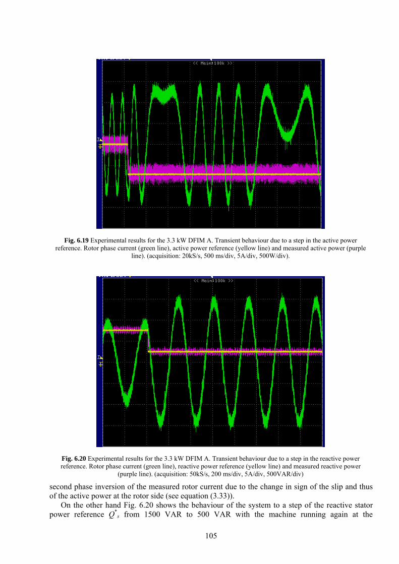
105
second phase inversion of the measured rotor current due to the change in sign of the slip and thus of the active power at the rotor side (see equation (3.33)).
On the other hand Fig. 6.20 shows the behaviour of the system to a step of the reactive stator power reference Q*
s from 1500 VAR to 500 VAR with the machine running again at the
Fig. 6.19 Experimental results for the 3.3 kW DFIM A. Transient behaviour due to a step in the active power reference. Rotor phase current (green line), active power reference (yellow line) and measured active power (purple
line). (acquisition: 20kS/s, 500 ms/div, 5A/div, 500W/div).
Fig. 6.20 Experimental results for the 3.3 kW DFIM A. Transient behaviour due to a step in the reactive power reference. Rotor phase current (green line), reactive power reference (yellow line) and measured reactive power
(purple line). (acquisition: 50kS/s, 200 ms/div, 5A/div, 500VAR/div)
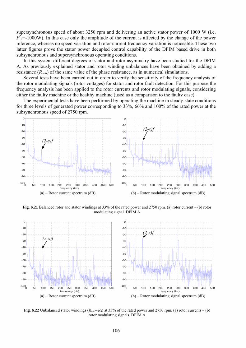
106
supersynchronous speed of about 3250 rpm and delivering an active stator power of 1000 W (i.e. P*
s=-1000W). In this case only the amplitude of the current is affected by the change of the power reference, whereas no speed variation and rotor current frequency variation is noticeable. These two latter figures prove the stator power decupled control capability of the DFIM based drive in both subsynchronous and supersynchronous operating conditions.
In this system different degrees of stator and rotor asymmetry have been studied for the DFIM A. As previously explained stator and rotor winding unbalances have been obtained by adding a resistance (Radd) of the same value of the phase resistance, as in numerical simulations.
Several tests have been carried out in order to verify the sensitivity of the frequency analysis of the rotor modulating signals (rotor voltages) for stator and rotor fault detection. For this purpose the frequency analysis has been applied to the rotor currents and rotor modulating signals, considering either the faulty machine or the healthy machine (used as a comparison to the faulty case).
The experimental tests have been performed by operating the machine in steady-state conditions for three levels of generated power corresponding to 33%, 66% and 100% of the rated power at the subsynchronous speed of 2750 rpm.
0 50 100 150 200 250 300 350 400 450 500-100
-90
-80
-70
-60
-50
-40
-30
-20
-10
0
frequency (Hz)
(2-s)f
(a) – Rotor current spectrum (dB)
0 50 100 150 200 250 300 350 400 450 500-100
-90
-80
-70
-60
-50
-40
-30
-20
-10
0
frequency (Hz)
(2-s)f
(b) – Rotor modulating signal spectrum (dB)
Fig. 6.21 Balanced rotor and stator windings at 33% of the rated power and 2750 rpm. (a) rotor current – (b) rotor
modulating signal. DFIM A
0 50 100 150 200 250 300 350 400 450 500-100
-90
-80
-70
-60
-50
-40
-30
-20
-10
0
frequency (Hz)
(2-s)f
(a) – Rotor current spectrum (dB)
0 50 100 150 200 250 300 350 400 450 500-100
-90
-80
-70
-60
-50
-40
-30
-20
-10
0
frequency (Hz)
(2-s)f
(b) – Rotor modulating signal spectrum (dB)
Fig. 6.22 Unbalanced stator windings (Radd=RS) at 33% of the rated power and 2750 rpm. (a) rotor currents – (b)
rotor modulating signals. DFIM A
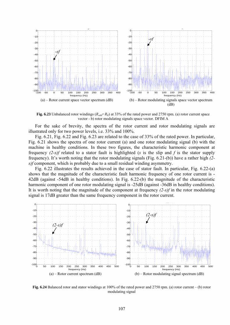
107
For the sake of brevity, the spectra of the rotor current and rotor modulating signals are illustrated only for two power levels, i.e. 33% and 100%.
Fig. 6.21, Fig. 6.22 and Fig. 6.23 are related to the case of 33% of the rated power. In particular, Fig. 6.21 shows the spectra of one rotor current (a) and one rotor modulating signal (b) with the machine in healthy conditions. In these two figures, the characteristic harmonic component at frequency (2-s)f related to a stator fault is highlighted (s is the slip and f is the stator supply frequency). It’s worth noting that the rotor modulating signals (Fig. 6.21-(b)) have a rather high (2-s)f component, which is probably due to a small residual winding asymmetry.
Fig. 6.22 illustrates the results achieved in the case of stator fault. In particular, Fig. 6.22-(a) shows that the magnitude of the characteristic fault harmonic frequency of one rotor current is -42dB (against -54dB in healthy conditions). In Fig. 6.22-(b) the magnitude of the characteristic harmonic component of one rotor modulating signal is -25dB (against -36dB in healthy conditions). It is worth noting that the magnitude of the component at frequency (2-s)f in the rotor modulating signal is 17dB greater than the same frequency component in the rotor current.
-100 -50 0 50 100 150 200 250 300 350 400-100
-90
-80
-70
-60
-50
-40
-30
-20
-10
0g
frequency (Hz)
-sf
(a) – Rotor current space vector spectrum (dB)
-100 -50 0 50 100 150 200 250 300 350 400-100
-90
-80
-70
-60
-50
-40
-30
-20
-10
0g
frequency (Hz)
-sf
(b) – Rotor modulating signals space vector spectrum
(dB)
Fig. 6.23 Unbalanced rotor windings (Radd=RR) at 33% of the rated power and 2750 rpm. (a) rotor current space vector - b) rotor modulating signals space vector. DFIM A
0 50 100 150 200 250 300 350 400 450 500-100
-90
-80
-70
-60
-50
-40
-30
-20
-10
0
frequency (Hz)
(2-s)f
(a) – Rotor current spectrum (dB)
0 50 100 150 200 250 300 350 400 450 500-100
-90
-80
-70
-60
-50
-40
-30
-20
-10
0dB FFT
frequency (Hz)
(2-s)f
(b) – Rotor modulating signal spectrum (dB)
Fig. 6.24 Balanced rotor and stator windings at 100% of the rated power and 2750 rpm. (a) rotor current – (b) rotor modulating signal
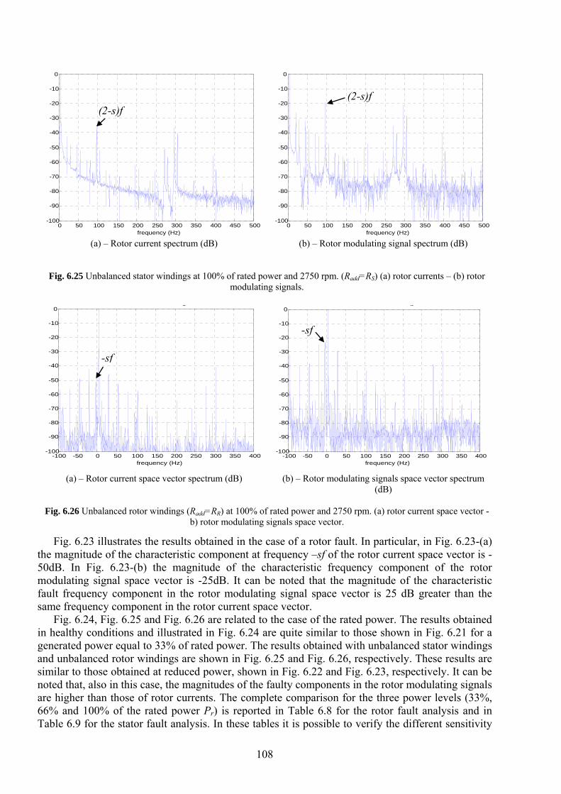
108
Fig. 6.23 illustrates the results obtained in the case of a rotor fault. In particular, in Fig. 6.23-(a) the magnitude of the characteristic component at frequency –sf of the rotor current space vector is -50dB. In Fig. 6.23-(b) the magnitude of the characteristic frequency component of the rotor modulating signal space vector is -25dB. It can be noted that the magnitude of the characteristic fault frequency component in the rotor modulating signal space vector is 25 dB greater than the same frequency component in the rotor current space vector.
Fig. 6.24, Fig. 6.25 and Fig. 6.26 are related to the case of the rated power. The results obtained in healthy conditions and illustrated in Fig. 6.24 are quite similar to those shown in Fig. 6.21 for a generated power equal to 33% of rated power. The results obtained with unbalanced stator windings and unbalanced rotor windings are shown in Fig. 6.25 and Fig. 6.26, respectively. These results are similar to those obtained at reduced power, shown in Fig. 6.22 and Fig. 6.23, respectively. It can be noted that, also in this case, the magnitudes of the faulty components in the rotor modulating signals are higher than those of rotor currents. The complete comparison for the three power levels (33%, 66% and 100% of the rated power Pr) is reported in Table 6.8 for the rotor fault analysis and in Table 6.9 for the stator fault analysis. In these tables it is possible to verify the different sensitivity
0 50 100 150 200 250 300 350 400 450 500-100
-90
-80
-70
-60
-50
-40
-30
-20
-10
0
frequency (Hz)
(2-s)f
(a) – Rotor current spectrum (dB)
0 50 100 150 200 250 300 350 400 450 500-100
-90
-80
-70
-60
-50
-40
-30
-20
-10
0
frequency (Hz)
(2-s)f
(b) – Rotor modulating signal spectrum (dB)
Fig. 6.25 Unbalanced stator windings at 100% of rated power and 2750 rpm. (Radd=RS) (a) rotor currents – (b) rotor modulating signals.
-100 -50 0 50 100 150 200 250 300 350 400-100
-90
-80
-70
-60
-50
-40
-30
-20
-10
0g
frequency (Hz)
-sf
(a) – Rotor current space vector spectrum (dB)
-100 -50 0 50 100 150 200 250 300 350 400-100
-90
-80
-70
-60
-50
-40
-30
-20
-10
0g
frequency (Hz)
-sf
(b) – Rotor modulating signals space vector spectrum
(dB)
Fig. 6.26 Unbalanced rotor windings (Radd=RR) at 100% of rated power and 2750 rpm. (a) rotor current space vector - b) rotor modulating signals space vector.
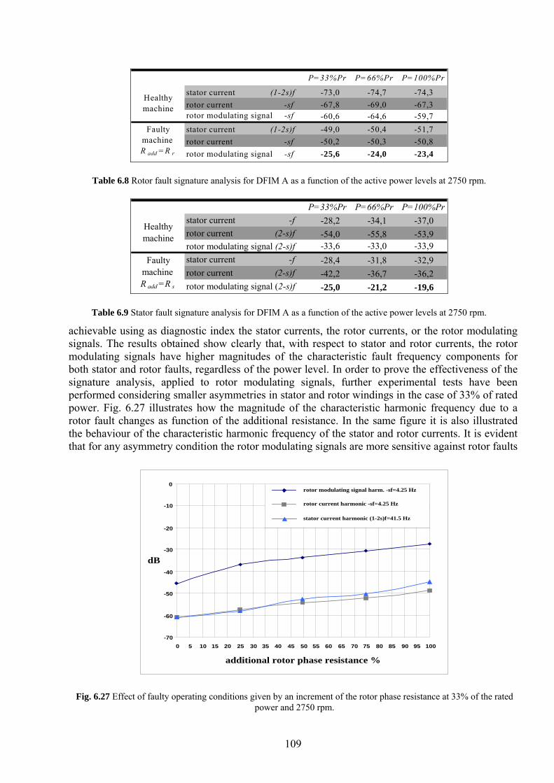
109
achievable using as diagnostic index the stator currents, the rotor currents, or the rotor modulating signals. The results obtained show clearly that, with respect to stator and rotor currents, the rotor modulating signals have higher magnitudes of the characteristic fault frequency components for both stator and rotor faults, regardless of the power level. In order to prove the effectiveness of the signature analysis, applied to rotor modulating signals, further experimental tests have been performed considering smaller asymmetries in stator and rotor windings in the case of 33% of rated power. Fig. 6.27 illustrates how the magnitude of the characteristic harmonic frequency due to a rotor fault changes as function of the additional resistance. In the same figure it is also illustrated the behaviour of the characteristic harmonic frequency of the stator and rotor currents. It is evident that for any asymmetry condition the rotor modulating signals are more sensitive against rotor faults
P=33%Pr P=66%Pr P=100%Pr
stator current (1-2s)f -73,0 -74,7 -74,3rotor current -sf -67,8 -69,0 -67,3rotor modulating signal -sf -60,6 -64,6 -59,7stator current (1-2s)f -49,0 -50,4 -51,7rotor current -sf -50,2 -50,3 -50,8rotor modulating signal -sf -25,6 -24,0 -23,4
Healthy machine
Faulty machine R add =R r
Table 6.8 Rotor fault signature analysis for DFIM A as a function of the active power levels at 2750 rpm.
P=33%Pr P=66%Pr P=100%Prstator current -f -28,2 -34,1 -37,0rotor current (2-s)f -54,0 -55,8 -53,9rotor modulating signal (2-s)f -33,6 -33,0 -33,9stator current -f -28,4 -31,8 -32,9rotor current (2-s)f -42,2 -36,7 -36,2rotor modulating signal (2-s)f -25,0 -21,2 -19,6
Healthy machine
Faulty machine R add =R s
Table 6.9 Stator fault signature analysis for DFIM A as a function of the active power levels at 2750 rpm.
-70
-60
-50
-40
-30
-20
-10
0
0 5 10 15 20 25 30 35 40 45 50 55 60 65 70 75 80 85 90 95 100
additional rotor phase resistance %
dB
rotor modulating signal harm. -sf=4.25 Hz
rotor current harmonic -sf=4.25 Hz
stator current harmonic (1-2s)f=41.5 Hz
Fig. 6.27 Effect of faulty operating conditions given by an increment of the rotor phase resistance at 33% of the rated
power and 2750 rpm.
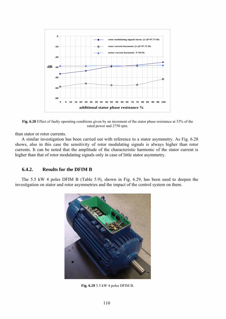
110
than stator or rotor currents. A similar investigation has been carried out with reference to a stator asymmetry. As Fig. 6.28
shows, also in this case the sensitivity of rotor modulating signals is always higher than rotor currents. It can be noted that the amplitude of the characteristic harmonic of the stator current is higher than that of rotor modulating signals only in case of little stator asymmetry.
6.4.2. Results for the DFIM B
The 5.5 kW 4 poles DFIM B (Table 5.9), shown in Fig. 6.29, has been used to deepen the investigation on stator and rotor asymmetries and the impact of the control system on them.
-60
-50
-40
-30
-20
-10
0
0 5 10 15 20 25 30 35 40 45 50 55 60 65 70 75 80 85 90 95 100
additional stator phase resistance %
dB
rotor modulating signals harm. (2-s)f=97.75 Hz
rotor current harmonic (2-s)f=97.75 Hz
stator current harmonic -f=50 Hz
Fig. 6.28 Effect of faulty operating conditions given by an increment of the stator phase resistance at 33% of the rated power and 2750 rpm.
Fig. 6.29 5.5 kW 4 poles DFIM B.
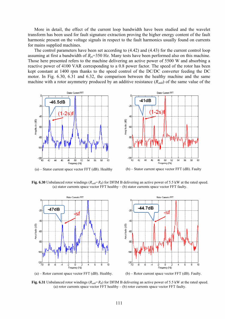
111
More in detail, the effect of the current loop bandwidth have been studied and the wavelet transform has been used for fault signature extraction proving the higher energy content of the fault harmonic present on the voltage signals in respect to the fault harmonics usually found on currents for mains supplied machines.
The control parameters have been set according to (4.42) and (4.43) for the current control loop assuming at first a bandwidth of Bpi=350 Hz. Many tests have been performed also on this machine. Those here presented refers to the machine delivering an active power of 5500 W and absorbing a reactive power of 4100 VAR corresponding to a 0.8 power factor. The speed of the rotor has been kept constant at 1400 rpm thanks to the speed control of the DC/DC converter feeding the DC motor. In Fig. 6.30, 6.31 and 6.32, the comparison between the healthy machine and the same machine with a rotor asymmetry produced by an additive resistance (Radd) of the same value of the
(a) – Stator current space vector FFT (dB). Healthy
(b) – Stator current space vector FFT (dB). Faulty
Fig. 6.30 Unbalanced rotor windings (Radd=RR) for DFIM B delivering an active power of 5.5 kW at the rated speed. (a) stator currents space vector FFT healthy – (b) stator currents space vector FFT faulty.
(a) – Rotor current space vector FFT (dB). Healthy.
(b) – Rotor current space vector FFT (dB). Faulty.
Fig. 6.31 Unbalanced rotor windings (Radd=RR) for DFIM B delivering an active power of 5.5 kW at the rated speed.
(a) rotor currents space vector FFT healthy – (b) rotor currents space vector FFT faulty.
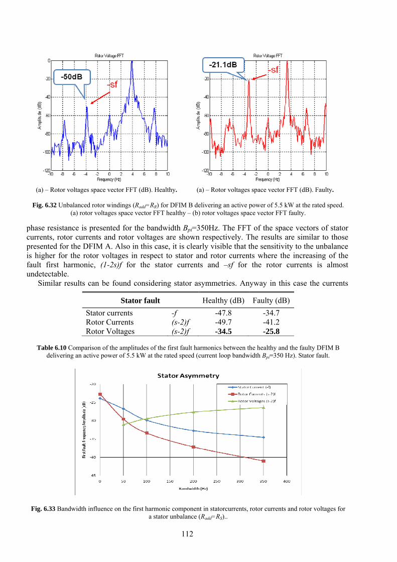
112
phase resistance is presented for the bandwidth Bpi=350Hz. The FFT of the space vectors of stator currents, rotor currents and rotor voltages are shown respectively. The results are similar to those presented for the DFIM A. Also in this case, it is clearly visible that the sensitivity to the unbalance is higher for the rotor voltages in respect to stator and rotor currents where the increasing of the fault first harmonic, (1-2s)f for the stator currents and –sf for the rotor currents is almost undetectable.
Similar results can be found considering stator asymmetries. Anyway in this case the currents
(a) – Rotor voltages space vector FFT (dB). Healthy.
(a) – Rotor voltages space vector FFT (dB). Faulty.
Fig. 6.32 Unbalanced rotor windings (Radd=RR) for DFIM B delivering an active power of 5.5 kW at the rated speed.
(a) rotor voltages space vector FFT healthy – (b) rotor voltages space vector FFT faulty.
Stator fault Healthy (dB) Faulty (dB) Stator currents -f -47.8 -34.7 Rotor Currents (s-2)f -49.7 -41.2 Rotor Voltages (s-2)f -34.5 -25.8
Table 6.10 Comparison of the amplitudes of the first fault harmonics between the healthy and the faulty DFIM B
delivering an active power of 5.5 kW at the rated speed (current loop bandwidth Bpi=350 Hz). Stator fault.
Fig. 6.33 Bandwidth influence on the first harmonic component in statorcurrents, rotor currents and rotor voltages for a stator unbalance (Radd=RS)..
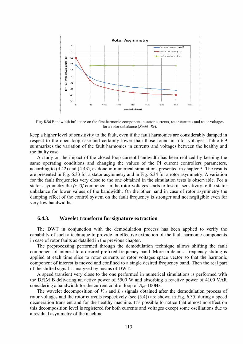
113
keep a higher level of sensitivity to the fault, even if the fault harmonics are considerably damped in respect to the open loop case and certainly lower than those found in rotor voltages. Table 6.9 summarizes the variation of the fault harmonics in currents and voltages between the healthy and the faulty case.
A study on the impact of the closed loop current bandwidth has been realized by keeping the same operating conditions and changing the values of the PI current controllers parameters, according to (4.42) and (4.43), as done in numerical simulations presented in chapter 5. The results are presented in Fig. 6.33 for a stator asymmetry and in Fig. 6.34 for a rotor asymmetry. A variation for the fault frequencies very close to the one obtained in the simulation tests is observable. For a stator asymmetry the (s-2)f component in the rotor voltages starts to lose its sensitivity to the stator unbalance for lower values of the bandwidth. On the other hand in case of rotor asymmetry the damping effect of the control system on the fault frequency is stronger and not negligible even for very low bandwidths.
6.4.3. Wavelet transform for signature extraction
The DWT in conjunction with the demodulation process has been applied to verify the capability of such a technique to provide an effective extraction of the fault harmonic components in case of rotor faults as detailed in the previous chapter.
The preprocessing performed through the demodulation technique allows shifting the fault component of interest to a desired prefixed frequency band. More in detail a frequency sliding is applied at each time slice to rotor currents or rotor voltages space vector so that the harmonic component of interest is moved and confined to a single desired frequency band. Then the real part of the shifted signal is analyzed by means of DWT.
A speed transient very close to the one performed in numerical simulations is performed with the DFIM B delivering an active power of 5500 W and absorbing a reactive power of 4100 VAR considering a bandwidth for the current control loop of Bpi=100Hz.
The wavelet decomposition of Vrsl and Irsl signals obtained after the demodulation process of rotor voltages and the rotor currents respectively (see (5.4)) are shown in Fig. 6.35, during a speed deceleration transient and for the healthy machine. It’s possible to notice that almost no effect on this decomposition level is registered for both currents and voltages except some oscillations due to a residual asymmetry of the machine.
Fig. 6.34 Bandwidth influence on the first harmonic component in stator currents, rotor currents and rotor voltages for a rotor unbalance (Radd=Rr).
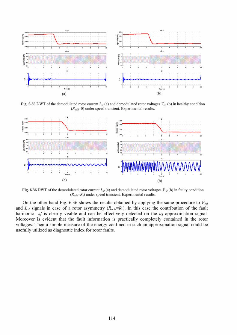
114
On the other hand Fig. 6.36 shows the results obtained by applying the same procedure to Vrsl and Irsl signals in case of a rotor asymmetry (Radd=Rr). In this case the contribution of the fault harmonic –sf is clearly visible and can be effectively detected on the a8 approximation signal. Moreover is evident that the fault information is practically completely contained in the rotor voltages. Then a simple measure of the energy confined in such an approximation signal could be usefully utilized as diagnostic index for rotor faults.
0 1 2 3 4 5 6 7 8 9 101280
1330
1380
1420- a -
Spee
d (r
pm)
0 1 2 3 4 5 6 7 8 9 10-2
0
2
- c -
Time (s)
a8
0 1 2 3 4 5 6 7 8 9 10-40
-20
0
20
40- b -
Cur
rent
s (A
)
(a)
0 1 2 3 4 5 6 7 8 9 101280
1330
1380
1420- a -
Spee
d (rp
m)
0 1 2 3 4 5 6 7 8 9 10-2
0
2
- c -
Time (s)
a8
0 1 2 3 4 5 6 7 8 9 10-40
-20
0
20
40- b -
Volta
ges
(V)
(b)
Fig. 6.35 DWT of the demodulated rotor current Irsl (a) and demodulated rotor voltages Vrsl (b) in healthy condition (Radd=0) under speed transient. Experimental results.
0 1 2 3 4 5 6 7 8 9 101280
1330
1380
1420- a -
Spee
d (rp
m)
0 1 2 3 4 5 6 7 8 9 10-2
0
2
- c -
Time (s)
a8
0 1 2 3 4 5 6 7 8 9 10-40
-20
0
20
40- b -
Cur
rent
s (A
)
(a)
0 1 2 3 4 5 6 7 8 9 101280
1330
1380
1420- a -
Spee
d (r
pm)
0 1 2 3 4 5 6 7 8 9 10-2
0
2
- c -
Time (s)
a8
0 1 2 3 4 5 6 7 8 9 10-40
-20
0
20
40- b -
Vol
tage
s (V
)
(b)
Fig. 6.36 DWT of the demodulated rotor current Irsl (a) and demodulated rotor voltages Vrsl (b) in faulty condition (Radd=Rr) under speed transient. Experimental results.
115
Conclusions
In this thesis rotor faults in squirrel cage induction motors and stator and rotor asymmetries in doubly fed induction generators have been investigated by taking into consideration the influence of the control system and non stationary operating conditions.
Suitable first harmonic models of both machines have been developed in order to deeply understand the machine behavior under faulty conditions. Subsequently these models have been coupled with the control structures based on field orientation typically employed in railway applications and in wind generation systems.
In this way the study of the behaviour of the entire variable speed drive under faulty conditions has been performed. Then three diagnostic procedures have been proposed, namely:
• The demodulation technique • The virtual current technique • The rotor modulating signal signature analysis.
The first one is a diagnostic procedure for rotor faults detection in squirrel cage induction machine-based drives under time-varying conditions. The method is tailored for railway applications where acceleration and deceleration transients occur frequently.
During transient operations torque and speed vary preventing the use of MCSA and of traditional spectral analysis for an effective diagnosis of rotor faults. Thanks to the proposed approach currents are demodulated in order to move time-varying components related to rotor faults to a single frequency.
Compared to solutions that use time-frequency distributions the proposed procedure requires simpler processing, moreover it exploits the observers of the drive control in order to achieve optimal demodulation results.
A diagnostic index is proposed, that is quite robust versus load and inertia variations and quite sensitive to provide an effective fault detection. Simulation and experimental results have been reported to confirm the validity of the proposed method.
The virtual current technique is a new model based procedure for the diagnosis of rotor faults in Direct Rotor Field Oriented Controlled Drives. The philosophy of the proposed diagnostic technique lies on the measurement of the oscillations at a frequency of 2sf present in the d-axis component of the estimated rotor flux of the motor. With this information, a virtual magnetizing current component associated with the fault is reconstructed. This signal, after its normalization using the average value of the torque-producing current component, allows the detection and quantification of the extension of rotor faults in the motor.
Simulation results obtained using two different versions of a DRFOC drive, as well as experimental results obtained with a DRFOC drive similar to the one usually found in traction drives for railway applications, demonstrate the effectiveness of the proposed method as a tool for the diagnosis of rotor faults in this type of system. Using the Virtual Current Technique it is possible to diagnose the fault in a way quite independent of the working conditions of the machine and of the control loop parameters. Moreover, most of the information needed for the implementation of this technique is already available inside the control system. No additional sensors besides the ones already inside the drive are needed. The Virtual Current Technique is an

116
attractive tool to be integrated into the control board of the drive, thus providing information about the condition of the motor in real-time.
Anyway the extraction of the 2sf component with variable reference flux is still an open issue that needs further investigations.
Finally the rotor modulating signals signature analysis has been presented as new and reliable diagnostic procedure for the characterization of stator and rotor faults in doubly fed induction generators. A stator flux oriented vector control has been implemented to control the DFIM by using a back-to-back converter connected between the rotor windings and the grid. This control system regulates the rotor currents in order to provide the desired active and reactive power from the stator side. In this sense the rotor current control loops will try to follow sinusoidal and balanced current references by applying unbalanced rotor voltages. Consequently, the typical rotor and stator current fault harmonic components might become less visible due to the compensating action of the control system. On the contrary, these fault harmonic components remain clearly observable in the rotor modulating signals and can be considered as a new effective diagnostic index for the detection of stator and rotor asymmetries in DFIMs.
Simulation and experimental results, carried out for different power levels and different current loop bandwidths, have proved that the rotor modulating signals have a higher sensitivity to stator and rotor asymmetries with respects to stator and rotor currents unless the bandwidth is extremely low.
Eventually an approach based on the Wavelet transform has been used to extract the fault signature information present on rotor voltages and currents, proving the higher sensitivity of the former and allowing an effective fault detection also in time varying conditions.
117
References
1. Bellini, A.; Filippetti, F.; Tassoni, C.; Capolino, G.-A.; , "Advances in Diagnostic Techniques for Induction Machines," Industrial Electronics, IEEE Transactions on , vol.55, no.12, Dec. 2008, pp.4109-4126
2. M. El Hachemi Benbouzid, “A review of induction motors signature analysis as a medium for faults detection”, IEEE Transactions on Industrial Electronics, vol. 47, no. 5, pp. 984–993, Oct. 2000.
3. S. Nandi, H. A. Toliyat, and X. Li, “Condition monitoring and fault diagnosis of electrical motors-a review”, IEEE Transaction on Energy Conversion, vol. 20, no. 4, Dec. 2005, pp. 719–729.
4. R. M. Tallam, S. B. Lee, G. C. Stone, G. B. Kliman, J. Yoo, T. G Habetler, and R. G. Harley, “A survey of methods for detection of stator-related faults in induction machines”, IEEE Transactions on Industry Applications, vol. 43, no. 4, Jul./Aug. 2007, pp. 920–933.
5. N. Bianchi, S. Bolognani, M. Zigliotto, and M. Zordan, “Innovative remedial strategies for inverter faults in IPM synchronous motor drives”, IEEE Transaction on Energy Conversion, vol. 18, no. 2, Jun. 2003, pp.-306–314.
6. L. Parsa and H. A. Toliyat, “Five-phase permanent-magnet motor-drives”, IEEE Transactions on Industry Applications, vol. 41, no. 1, Jan./Feb. 2005, pp. 30–37.
7. A. H. Bonnett and C. Yung, “Increased efficiency versus increased reliability”, IEEE Industry Applications Magazine, vol. 14, no. 1, Jan./Feb. 2008, pp. 29–36.
8. P. Vas, “Parameter estimation, condition monitoring, and diagnosis of electrical machines”, Oxford, U.K. Clarendon Press, 2001. IEEE Industry Applications Magazine, vol. 33, no. 1, Jan./Feb. 1997, pp. 24–34.
9. C. M. Riley, B. K. Lin, T. G. Habetler, and R. R. Schoen, “A method for sensorless on-line vibration monitoring of induction machines”, IEEE Transactions on Industry Applications, vol. 34, no. 6, Nov./Dec. 1998, pp. 1240–1245.
10. M. E. Badaoui, F. Guillet, and J. Danire, “New applications of the-real cepstrum to gear signals, including definition of a robust fault indicator”, Mechanical Systems and Signal Processing, vol. 18, no. 5, 2004, pp. 1031–1046.
11. R. Ong, J. H. Dymond, and R. D. Findlay, “Bearing damage analysis in a large oil-ring-lubricated induction machine”, IEEE Transactions on Industrial Electronics, vol. 47, no. 5, Oct. 2000, pp. 1085–1091.
12. D. G. Dorrell, W. T. Thomson, and S. Roach, “Combined effects of static and dynamic eccentricity on air gap flux waves and the application of current monitoring to detect
118
dynamic eccentricity in 3-phase induction motors”, in Electrical Machines and Drives, 1995-Seventh International Conference on (Conf. Publ. No. 412), Durham, UK, Sep. 1995, pp. 151–155.
13. C. Gerada, K. J. Bradley, M. Sumner, P. Wheeler, S. Pickering, J. Clare, C. Whitley, and G. Towers, “The results do mesh”, IEEE Industry Applications Magazine, vol. 13, no. 2, pp. 62–72, Mar./Apr. 2007.
14. J. L. Kohler, J. Sottile, and F. C. Trutt, “Alternatives for assessing the electrical integrity of induction motors”, IEEE Transactions on Industry Applications, vol. 28, no. 5, pp. 1109–1117, Sep./Oct. 1992.
15. J. L. Kohler, J. Sottile, and F. C. Trutt, “Condition monitoring of stator windings in induction motors. I. experimental investigation of the effective negative-sequence impedance detector”, IEEE Transactions on Industry Applications, vol. 38, no. 5, pp. 1447–1453, Sep./Oct. 2002.
16. J. Sottile, F. C. Trutt, and J. L. Kohler, “Condition monitoring of stator windings in induction motors. II. experimental investigation of voltage mismatch detectors”, IEEE Transactions on Industry Applications, vol. 38, no. 5, pp. 1454–1459, Sep./Oct. 2002.
17. S. B. Lee, R. M. Tallam, and T. G. Habetler, “A robust, on-line turn fault detection technique for induction machines based on monitoring the sequence component impedance matrix”, IEEE Transactions on Power Electronics, vol. 18, no. 3, pp. 865–872, May 2003.
18. F. Filippetti, G. Franceschini, C. Tassoni, S. Meo, and A. Ometto, “A simplified model of induction motor with stator shorted turns oriented to diagnostics”, in Proc. Int. Conf. Elect. Mach, ICEM, 1996, pp. 410– 413.
19. S. Grubic, J.M. Aller, B.Lu, T.G Habetler, "A survey of testing and monitoring methods for stator insulation systems in induction machines," Condition Monitoring and Diagnosis, 2008. CMD 2008. International Conference on , vol., no., pp.196-203, 21-24 April 2008
20. D. Kostic-Perovic, M. Arkan, and P. Unsworth, “Induction motor fault detection by space vector angular fluctuation”, in Industry Applications Conference, 2000. Conference Record of the 2000 IEEE, vol. 1, Rome, Italy, 2000, pp. 388–394.
21. A. Bellini, C. Concari, G. Franceschini, E. Lorenzani, and C. Tassoni, “Induction drives diagnosis by signal injection technique: Effectiveness and severity classification”, in IEEE IEMDC05, International Electric Machines and Drives Conference, San Antonio, TX, USA, May 2005.
22. F. Briz, M. W. Degner, A. B. Diez, and J. M. Guerrero, “Online diagnostics in inverter-fed induction machines using high-frequency signal injection”, IEEE Transactions on Industry Applications, vol. 40, no. 4, pp. 1153–1161, July/Aug. 2004
23. P. Garcia, F. Briz, M. W. Degner, and D. Diaz-Reigosa, “Accuracy, bandwidth, and stability limits of carrier-signal-injection-based sensorless control methods”, IEEE Transactions on Industry Applications, vol. 43, no. 4, pp. 990–1000, Jul./Aug. 2007.
24. A. Bellini, F. Filippetti, G. Franceschini, C. Tassoni, and G. B. Kliman”, Quantitative evaluation of induction motor broken bars by means of electrical signature analysis”, IEEE Transactions on Industry Applications, vol. 37, no. 5, pp. 1248–1255, Sept./Oct. 2001.
119
25. F. Filippetti, G. Franceschini, C. Tassoni, and P. Vas, “AI techniques in induction machines diagnosis including the speed ripple effect”, IEEE Trans. on Ind. Appl., vol. 34, no. 1, pp. 98–108, Jan./Feb. 1998.
26. F. Filippetti, M. Martelli, G. Franceschini, and C. Tassoni, “Development of expert system knowledge base to on-line diagnosis of rotor electrical faults of induction motors”, in Industry Applications Society Annual Meeting, 1992., Conference Record of the 1992 IEEE, Houston, TX, USA, Oct. 1992, pp. 92–99.
27. A. Bellini, F. Filippetti, G. Franceschini, C. Tassoni, R. Passaglia, M. Saottini, G. Tontini, M. Giovannini, and A. Rossi, “On-field experience with online diagnosis of large induction motors cage failures using MCSA”, IEEE Transactions on Industry Applications, vol. 38, no. 4, pp. 1045–1053, Jul./Aug. 2002.
28. A. Bellini, C. Concari, G. Franceschini, E. Lorenzani, C. Tassoni, and A. Toscani, “Virtual inertia test bed for quantification of sideband currents in induction machines diagnostics”, in ICEM 2006, 2006
29. C. Kral, R. S. Wieser, F. Pirker, and M. Schagginger, “Sequences of field-oriented control for the detection of faulty rotor bars in induction machines-the Vienna monitoring method”, IEEE Transactions on Industrial Electronics, vol. 47, no. 5, pp. 1042–1050, Oct. 2000
30. F. Filippetti, G. Franceschini, C. Tassoni, and P. Vas, “Broken bar detection in induction machines: comparison between current spectrum approach and parameter estimation approach”, in Industry Applications Society Annual Meeting, 1994, Conference Record of the 1994 IEEE, Denver, CO, USA, Oct. 1994, pp. 95–102.
31. Z. Liu, X. Yin, Z. Zhang, D. Chen, and W. Chen, “Online rotor mixed fault diagnosis way based on spectrum analysis of instantaneous power in squirrel cage induction motors”, IEEE Transactions on Energy Conversion, vol. 19, no. 3, pp. 485–490, Sep. 2004.
32. A. Bellini, F. Filippetti, G. Franceschini, N. Petrolini, and C. Tassoni, “On-line diagnosis in induction drives rotor by signal injection technique: Fault localisation and severity classification”, IEEE SDEMPED, pp. 531–536, 2001.
33. H. A. Toliyat and T. A. Lipo, “Transient analysis of cage induction machines under stator, rotor bar and end ring faults,” IEEE Transaction on Energy Conversion, vol. 10, no. 2, pp. 241–247, Jun. 1995.
34. M.F. Cabanas, F. Pedrayes, M.R. Gonzalez, M.G. Melero, C.H. Rojas, G.A. Orcajo, J.M. Cano, F. Nuno, "A new electronic instrument for the early detection of broken rotor bars in asynchronous motors working under arbitrary load conditions," Diagnostics for Electric Machines, Power Electronics and Drives, 2005. SDEMPED 2005. 5th IEEE International Symposium on , vol., no., pp.1-6, 7-9 Sept. 2005
35. C.-E. Kim, Y.-B. Jung, S.-B. Yoon, and D.-H. Im, “The fault diagnosis of rotor bars in squirrel cage induction motors by time-stepping finite element method,” IEEE Transactions on Magnetics, vol. 33, pp. 2131-2134, Mar. 1997.
36. P. Vas, F. Filippetti, G. Franceschini, and C. Tassoni, “Transient modeling oriented to diagnostics of induction machines with rotor asymmetries”, in Proc. ICEM 1994, Paris, France, 1994.
120
37. R. Datta, and V. T. Ranganathan, “Variable-speed wind power generation using doubly fed wound rotor induction machine- A comparison with alternative schemes”, IEEE Trans. on Energy Conversion, vol. 17, n° 3, Sept. 2002, pp. 414-421.
38. Y. Tang, and L. Xu, “A flexible active and reactive power control strategy for a variable speed constant frequency generating system”, IEEE Trans. on Energy Conversion, vol. 10, n° 4, July 1995, pp. 472-478.
39. A. Tapia, G. Tapia, J. X. Ostolaza, and J. R. Saenz, “Modeling and control of a wind turbine driven doubly fed induction generator”, IEEE Trans. on Energy Conversion, vol. 18, n° 2, June 2003, pp. 194-204.
40. R. Pena, J. C. Clare, and G. M. Asher, “Doubly fed induction generator using back-to-back PWM converters and its applications to variable speed wind-energy generation,” Inst. Elec. Eng. Proc. Electric Power Applications, vol. 143, no. 3, pp. 231–241, May 1996.
41. E. Bogalecka and Z. Kzreminski, “Control system of a doubly-fed induction machine supplied by current controlled voltage source inverter,” in Proc. Inst. Elec. Eng. of Sixth Int. Conf. on Electrical Machines and Drives, London, U.K., 1993.
42. Malinowski, M.; Kazmierkowski, M.P.; Trzynadlowski, A.M., "A comparative study of control techniques for PWM rectifiers in AC adjustable speed drives," Power Electronics, IEEE Transactions on, vol.18, no.6, pp. 1390- 1396, Nov. 2003.
43. J. Holtz, “Sensorless control of induction motor drives”, Proceedings of the IEEE, vol. 90, no. 8, pp. 1359–1394, Aug. 2002.
44. P. H. Mellor, T. J. Allen, R. Ong, and Z. Rahma, “Faulted behaviour of permanent magnet electric vehicle traction drives”, in Electric Machines and Drives Conference, 2003. IEMDC’03. IEEE International, vol. 1, June 2003, pp. 554–558.
45. M. W. Winterling, E. Tuinman, and W. Deleroi, “Fault analysis of electromechanical traction drives”, in Electrical Machines and Drives, 1997 Eighth International Conference on (Conf. Publ. No. 444), Cambridge, UK, Sept. 1997, pp. 248–252.
46. C. Kral, F. Pirker, and G. Pascoli, “Detection of rotor faults in inverter fed induction machines by means of the Vienna monitoring method - a proposed application for traction drives”, in Conferences Proceedings of the first International Conference on Railway Traction Systems, RTS 3, Capri, Italy, May 2001, pp. 79–89.
47. H. Henao, H. Razik, and G. A. Capolino, “Analytical approach of the stator current frequency harmonics computation for detection of induction machine rotor faults”, IEEE Transactions on Industry Applications, vol. 41, no. 3, pp. 801–807, May/June 2005.
48. J. H. Jung, J. J. Lee, and B. H. Kwon, “Online diagnosis of induction motors using MCSA”, IEEE Transactions on Industrial Electronics, vol. 53, no. 6, pp. 1842–1852, Dec. 2006.
49. R. R. Schoen and T. G. Habetler, “Effects of time-varying loads on rotor fault detection in induction machines”, IEEE Transactions on Industry Applications, vol. 31, no. 4, pp. 900–906, July/Aug. 1995.
50. R. S.Wieser, C. Kral, and F. Pirker, “The Vienna induction machine monitoring method; on the impact of the field oriented control structure on real operational behavior of a faulty machine”, in Industrial Electronics Society, 1998. IECON ’98. Proceedings of the 24th Annual Conference of the IEEE, vol. 3, Aachen, Aug. /Sept. 1998, pp. 1544–1549.
121
51. A. Bellini, F. Filippetti, G. Franceschini, and C. Tassoni, “Closed loop control impact on the diagnosis of induction motors faults”, IEEE Transactions on Industry Applications, vol. 36, no. 5, pp. 1318–1329,Sept./Oct. 2000.
52. D. Casadei, F. Filippetti, C. Rossi, A. Stefani, A. Yazidi, and G. A.Capolino, “Diagnostic technique based on rotor modulating signals signature analysis for doubly fed induction machines in wind generator systems”, in Industry Applications Conference, 2006. 41st IAS Annual Meeting. Conference Record of the 2006 IEEE, vol. 3, Tampa, FL, Oct.2006, pp. 1525–1532.
53. I. Jaksch, “Faults diagnosis of three-phase induction motors using envelope analysis”, in Diagnostics for Electric Machines, Power Electronics and Drives, 2003. SDEMPED 2003. 4th IEEE International Symposium on, Aug. 2003, pp. 289–293.
54. S. H. Kia, H. Henao, and G. A. Capolino, “A high-resolution frequency estimation method for three-phase induction machine fault detection”, IEEE Transactions on Industrial Electronics, vol. 54, no. 4, pp. 2305–2314, Aug. 2007.
55. S. Rajagopalan, J. M. Aller, J. A. Restrepo, T. G. Habetler, and R. G. Harley, “Detection of rotor faults in brushless DC motors operating under nonstationary conditions”, IEEE Transactions on Industry Applications, vol. 42, no. 6, pp. 1464–1477, Nov./Dec. 2006.
56. M. Blodt, D. Bonacci, J. Regnier, M. Chabert, and J. Faucher, “Online monitoring of mechanical faults in variable-speed induction motor drives using the Wigner distribution”, IEEE Transactions on Industrial Electronics, vol. 55, no. 2, pp. 522–533, Feb. 2008.
57. L. Eren and M. J. Devaney, “Motor bearing damage detection via wavelet analysis of the starting current transient”, in Instrumentation and Measurement Technology Conference, 2001. IMTC 2001. Proceedings of the 18th IEEE, vol. 3, Budapest, Hungary, 2001, pp. 1797–1800.
58. H. Douglas, P. Pillay, and A. K. Ziarani, “A new algorithm for transient motor current signature analysis using wavelets”, IEEE Transactions on Industry Applications, vol. 40, no. 5, pp. 1361–1368, Sept./Oct. 2004.
59. H. Douglas, P. Pillay, and A. K. Ziarani, “Broken rotor bar detection in induction machines with transient operating speeds”, IEEE Transaction on Energy Conversion, vol. 20, no. 1, pp. 135–141, Mar. 2005.
60. J. Cusido, L. Romeral, J. A. Ortega, J. A. Rosero, and A. Garcia Espinosa, “Fault detection in induction machines using power spectral density in wavelet decomposition”, IEEE Transactions on Industrial Electronics, vol. 55, no. 2, pp. 633–643, Feb. 2008.
61. A. Stefani, F. Filippetti, and A. Bellini, “Diagnosis of induction machines in time-varying conditions”, in Diagnostics for Electric Machines, Power Electronics and Drives, 2007. SDEMPED 2007. IEEE International Symposium on, Cracow, Poland, Sept. 2007, pp. 126–131.
62. H. Henao, C. Martis, and G. A. Capolino, “An equivalent internal circuit of the induction machine for advanced spectral analysis”, IEEE Transactions on Industry Applications, vol. 40, no. 3, pp. 726–734, May/June 2004.
63. X. Tu, L. A. Dessaint, M. El Kahel, and A. O. Barry, “A new model of synchronous machine internal faults based on winding distribution”, IEEE Transactions on Industrial Electronics, vol. 53, no. 6, pp. 1818–1828, Dec. 2006.
122
64. G. Didier, E. Ternisien, O. Caspary, and H. Razik, "Fault detection of broken rotor bars in induction motor using a global fault index”, IEEE Transactions on Industry Applications, vol. 42, pp. 79-88, January/February 2006.
65. L. Wu, T. Habetler, and R. Harley, "A Review of Separating Mechanical Load Effects from Rotor Faults Detection in Induction Motors”, in Proc. IEEE SDEMPED, 2007, pp. 221-225.
66. A. M. Trzynadlowski and E. Ritchie, "Comparative investigation of diagnostic media for induction motors: a case of rotor cage faults”, IEEE Transactions on Industrial Electronics, vol. 47, pp. 1092-1099, October 2000.
67. T. Wolbank, J. Machl, R. Woehrnschimmel, and R. Schneiderbauer, "Low-cost inverter based detection of rotor faults in induction machines for quality management systems”, in Proc. IEEE IECON, 2004, pp. 324-329.
68. B. Mirafzal and N. A. O. Demerdash, "Effects of load magnitude on diagnosing broken bar faults in induction motors using the pendulous oscillation of the rotor magnetic field orientation”, IEEE Transactions on Industry Applications, vol. 41, pp. 771-783, May/June 2005.
69. S. M. A. Cruz and A. J. M. Cardoso, "Diagnosis of Rotor Faults in Closed-Loop Induction Motor Drives”, in Proc. IEEE IAS Annual Meeting, 2006, pp. 2346-2353.
70. S. M. A. Cruz and A. J. M. Cardoso, "Fault Indicators for the Diagnosis of Rotor Faults in FOC Induction Motor Drives”, in Proc. IEEE IEMDC, Antalya, Turkey, 2007, pp. 1136-1141.
71. C. C. Martins Cunha and B. J. Cardoso Filho, "Detection of Rotor Faults in Squirrel-Cage Induction Motors using Adjustable Speed Drives”, in Proc. IEEE IAS Annual Meeting, 2006, pp. 2354-2359.
72. S. M. A. Cruz, H. A. Toliyat, and A. J. M. Cardoso, "DSP implementation of the multiple reference frames theory for the diagnosis of stator faults in a DTC induction motor drive”, IEEE Transactions on Energy Conversion, vol. 20, pp. 329-335, June 2005.
73. B. Akin, U. Orguner, H. A. Toliyat, and M. Rayner, "Phase-Sensitive Detection of Motor Fault Signatures in the Presence of Noise”, IEEE Transactions on Industrial Electronics, vol. 55, pp. 2539-2550, June 2008.
74. C. Kral, F. Pirker, and G. Pascoli, "Model-based detection of rotor faults without rotor position sensor - the sensorless Vienna monitoring method”, IEEE Transactions on Industry Applications, vol. 41, pp. 784-789, May/June 2005.
75. S. M. A. Cruz and A. J. M. Cardoso, "Diagnosis of rotor faults in direct and indirect FOC induction motor drives”, in Proc. EPE, Aalborg, Denmark, 2007, pp. 1-10.
76. A. Bellini, C. Concari, G. Franceschini, and C. Tassoni, "Different Procedures for the Diagnosis of Rotor Fault in Closed Loop Induction Motors Drives”, in Proc. IEEE IEMDC, Antalya, Turkey, 2007, pp.1427-1433.
77. S. M. A. Cruz and A. J. M. Cardoso, "Analysis and diagnosis of rotor faults in high-performance induction motor drives”, in International Conference on Electric Machines, Chania, Crete Island, Greece, 2006
123
78. Y. Zhongming, W. Bin, and A. Sadeghian, "Current signature analysis of induction motor mechanical faults by wavelet packet decomposition," IEEE Transactions on Industrial Electronics, vol. 50, pp. 1217-1228, December 2003.
79. J. A. Antonino-Daviu, M. Riera-Guasp, J. R. Folch, and M. P. M. Palomares, "Validation of a new method for the diagnosis of rotor bar failures via wavelet transform in industrial induction machines," IEEE Transactions on Industry Applications, vol. 42, pp. 990-996, July/August 2006.
80. B. Ayhan, M. Y. Chow, and M. H. Song, "Multiple Discriminant Analysis and Neural-Network-Based Monolith and Partition Fault- Detection Schemes for Broken Rotor Bar in Induction Motors," IEEE Transactions on Industrial Electronics, vol. 53, pp. 1298-1308, August 2006.
81. S. B. Makarand, J. K. Zafar, M. S. Hiralal, and L. S. Ram, "Adaptive Neural Fuzzy Inference System for the Detection of Inter-Turn Insulation and Bearing Wear Faults in Induction Motor," IEEE Transactions on Industrial Electronics, vol. 54, pp. 250-258, February 2007.
82. S. Hua and C. Kil To, "Induction Machine Condition Monitoring Using Neural Network Modeling," IEEE Transactions on Industrial Electronics, vol. 54, pp. 241-249, February 2007.
83. M. Haji and H. A. Toliyat, "Pattern recognition-a technique for induction machines rotor broken bar detection," IEEE Transactions on Energy Conversion, vol. 16, pp. 312-317, December 2001.
84. L. A. Pereira and D. da Silva Gazzana, "Rotor broken bar detection and diagnosis in induction motors using stator current signature analysis and fuzzy logic," in Proc. IEEE IECON 2004, 2004, pp. 3019-3024.
85. A. Bellini, F. Filippetti, G. Franceschini, and C. Tassoni, "Classification of diagnostic indexes for field oriented induction motor drives," in Proc. IEEE SDEMPED, Atlanta, GA, USA, 2003, pp. 217-222.
86. A. Bellini, G. Franceschini, C. Tassoni, and A. A. T. A. Toscani, "Assessment of induction machines rotor fault severity by different approaches," in Proc. IEEE IECON, Raleigh, USA, 2005, pp. 1461-1466.
87. A. Bellini, C. Concari, G. Franceschini, E. Lorenzani, C. Tassoni, and A. Toscani, "Thorough Understanding and Experimental Validation of Current Sideband Components in Induction Machines Rotor Monitoring," in Proc. IEEE IECON 2006, 2006, pp. 4957-4962.
88. A. Bellini, F. Filippetti, G. Franceschini, T. Sobczyk, and C. Tassoni,"Diagnosis of induction machines by d-q and i.s.c. rotor models," in Proc. IEEE SDEMPED, Vienna, Austria, 2005, pp. 1-6.
89. L. Xiaogang, L. Yuefeng, H. A. Toliyat, A. El-Antably, and T. A. Lipo, "Multiple coupled circuit modeling of induction machines," IEEE Transactions on Industry Applications, vol. 31, pp. 311-318, 1995.
90. S. M. A. Cruz and A. J. M. Cardoso, "Modelling and simulation of stator winding faults in three-phase induction motors, including rotor skin effect," in International Conference on Electric Machines, Brugge, Belgium, 2002, pp. 1-6.
124
91. D. Jovcic, "Phase locked loop system for FACTS," IEEE Transactions on Power Systems, vol. 18, pp. 1116-1124, August 2003.
92. S. M. A. Cruz and A. J. M. Cardoso, "Rotor cage fault diagnosis in three-phase induction motors by the synchronous reference frame current Park's Vector Approach," in International Conference on Electric Machines, Espoo, Finland, 2000, pp. 776-780.
93. I. Albizu, A. Tapia, J. R. Saenz, A. J. Mazon, and I. Zamora, “On-line stator winding fault diagnosis in induction generators for renewable generation”, in Proc. of the 12th IEEE Mediterranean Electrotechnical Conference, MELECON 2004, Dubrovnik, Croatia, 12-15 May 2004, vol. 3, pp. 1017-1020.
94. L. M. Popa, B. Bak-Jensen, E. Ritchie, and I. Boldea, “Condition monitoring of wind generators”, in Conference Record of the 38th IAS Annual Meeting, Seattle, USA, 12-16 Oct. 2003, vol. 3, pp.1839–1846.
95. Q.F. Lu, Z.T. Cao, and E. Ritchie, “Model of stator inter-turn short circuit fault in doubly-fed induction generators for wind turbine”. in Proc. IEEE 35th Annual Power Electronics Specialists Conference PESC’04, Aachen, Germany, 20-24 June 2004, vol. 2, pp. 932–937.
96. J. Penman, H.G. Sedding, B.A. Lloyd, and W.T. Fink, “Detection and location of inter-turn short-circuits in the stator windings of operating motors”, IEEE Trans. on Energy Conversion, vol. 9, n° 4, Dec.1994, pp. 652-658.
97. A. Yazidi, H. Henao, G. A. Capolino, M. Artioli, F. Filippetti, and D.Casadei, “Flux signature analysis: an alternative method for fault diagnosis of induction machines”, in Proc. IEEE PowerTech’05, St.Petersburg, Russia, June 2005, CD-ROM, paper n°424, 6 pages.
98. D. Casadei, F. Filippetti, C. Rossi, A. Stefani, and A. Yazidi, “Experimental characterization of electrical faults in a doubly-fed induction machine (DFIM) for wind power generation”, in Proc. of International Conference on Power Electronics and Intelligent Control for Energy Conservation, PELINCEC’05, Warsaw, Poland, 16-19 Oct. 2005, paper ID: 255.
99. A. Yazidi, H. Henao, G.A. Capolino, D. Casadei, and F. Filippetti, “Double-Fed Three-Phase Induction Machine abc Model for Simulation and Control Purposes”, in Proc. of the 24th Annual Conference of the IEEE Industrial Electronics Society, IECON 2005, Raleigh, USA, 6-10 Nov. 2005.
100. A. Yazidi, G.A. Capolino, D. Casadei, F. Filippetti, and C. Rossi, “Simulation of a Doubly-Fed Induction Machine for wind turbine generator Fault Analysis”, in Proc. 5th IEEE Int. Symp. on Diagnostics for Electric Machines, Power Electronics and Drives, SDEMPED 2005, Vienna, Austria, 7-9 Sept. 2005, CD-ROM. ISBN 0-7803-9123-X, pp. 279-284.
101. Bellini, A.; , "Quad Demodulation: A Time Domain Diagnostic Method for Induction Machines," Industry Applications Conference, 2007. 42nd IAS Annual Meeting. Conference Record of the 2007 IEEE, vol., no., pp.2249-2253, 23-27 Sept. 2007.
102. Cruz, S.M.A.; Stefani, A.; Filippetti, F.; Cardoso, A.J.M.;"Diagnosis of rotor faults in traction drives for railway applications," Electrical Machines, 2008. ICEM 2008. 18th International Conference on, vol., no., pp.1-6, 6-9 Sept. 2008.
103. S. Rajagopalan, J.M. Aller, J.A. Restrepo, T.G. Habetler, R.G. Harley, "Analytic-Wavelet-Ridge-Based Detection of Dynamic Eccentricity in Brushless Direct Current
125
(BLDC) Motors Functioning Under Dynamic Operating Conditions", IEEE Trans. on Ind. Elec, Vol. 54, N° 3, pp. 1410–1419, June 2007.
104. A. Ordaz-Moreno, R.J.Romero-Troncoso, J. A. Vite-Frias, J. R. Rivera-Gillen, and A. Garcia-Perez, "Automatic Online Diagnosis Algorithm for Broken-Bar Detection on Induction Motors Based on Discrete Wavelet Transform for FPGA Implementation", IEEE Trans. on Ind. Elec., Vol. 55, N° 5, pp. 1361–1368, May. 2008.
105. J.A. Daviu, P.J. Rodriguez, M.R. Guasp, M. P. Sanchez, A. Arkkio, ''Detection of combined faults in induction machines with stator parallel branches through the DWT of the start-up current'', Journal of Mechanical Systems and Signal Processing, accepted in Feb. 2009.
106. W.T. Thomson and M. Fenger, “Current Signature Analysis to Detect Induction Motor Faults”, IEEE Industry Applications Magazine, pp. 26-34, July/August 2001.
107. Y. Gritli, A. Stefani, F. Filippetti and A. Chatti, "Stator fault analysis based on Wavelet technique for wind turbines equipped with DFIG", ICCEP’09, pp 485-491. Italy, June 2009.
108. T.K. Sarkar, C. Su, R. Adve, M.S. Palma, L.G. Castillo, R. Boix, "A Tutorial on Wavelets from an Electrical Engineering Perspective, Part 1: Discrete Wavelet Techniques", IEEE Ante. and Prop. Mag., Vol. 40, N° 5, Oct. 1998.
109. Gritli, Y.; Stefani, A.; Rossi, C.; Filippetti, F.; Chatti, A.; , "Doubly Fed Induction Machine stator fault diagnosis under time-varying conditions based on frequency sliding and wavelet analysis," Diagnostics for Electric Machines, Power Electronics and Drives, 2009. SDEMPED 2009. IEEE International Symposium on , vol., no., pp.1-7, Aug. 31 20096-Sept. 3 2009.
110. Gritli, Y.; Stefani, A.; Filippetti, F.; Chatti, A.; , "Stator fault analysis based on wavelet technique for wind turbines equipped with DFIG," Clean Electrical Power, 2009 International Conference on , vol., no., pp.485-491, 9-11 June 2009.

Acknowledgements
My first thought goes to my parents. Without them this work would not exist. They gave all the support to accomplish my objectives and many other things more.
My gratitude goes also to all the people I met during my path towards the Ph.D. degree. My experience in France gave me the opportunity to know all the guys from the “Happy Team”. Gustavo, Juan and their families, Manes, Manolo, Carlos with his Jose Antonio brothers, Sergio who gave an important contribution to my work, Matteo who tried to teach me cooking, Marc, Wojciech, Grzegorz, Arthur, Jarek, Tarik, Julie, Hubert and Piotr.
I want to thank also the people who confirmed to be a constant during these three years and the new one I met during my second stay in Bologna. I refer to all the old friends of Rimini (Belmurri and Louthe first of all) and all the new friends from Teramo and surroundings. Thanks Gennaro, Luisa, Fonzie, Antonio, Valentina and Amedeo because you had to tolerate my disorder at home and because you made me not starve (I could not live only eating tuna and corn).
I want also to thank all the guys from the private and semi unauthorized canteen at the Department of Electrical Engineering who made become a pleasure the days spent in the lab during this working period.
Finally my gratitude goes also to Professor Fiorenzo Filippetti for the help he provided to me as my tutor and who gave me the possibility to attend Ph.D. courses. Moreover, I have to thank Domenico Casadei, Giovanni Serra, Angelo Tani, and most of all Luca Zarri who was always available for precious suggestions and who was able to solve most of my professional and non professional doubts.
Thanks to all the people I forgot to remember (I’m sure there are many)
Thanks to everyone
Andrea