Embed Size (px)
Citation preview
INDUSTRIAL ORGANIZATION
PERFECT COMPETITIONChapter 12
Costs and Supply Decisions
• How much should a firm supply?• Firms and their managers should attempt to maximize profits
(Profits = Revenues – Costs)• Select a pricing strategy that induces a demand for a product that
generates highest revenue relative to the cost of production of that level of supply.
• Profits depends on response of revenues to changes in production quantities.
Perfect Competition/ Price Taking• We think of some markets as characterized by perfect
competition• In competitive markets, no firm has the market power to set their
own price.
• Firms in perfectly competitive markets take their price as given.
China Price Download
Characteristics of Competitive Markets• Non-differentiated goods• Large number of firms• All firms are small relative to the market• Free entry and exit.
MES and Market Structure
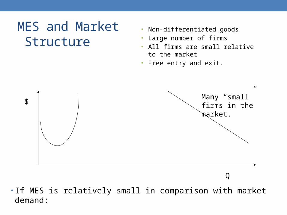
• If MES is relatively small in comparison with market demand:
$
Q
Many “small” firms in the market.
• Non-differentiated goods• Large number of firms• All firms are small relative to the market• Free entry and exit.
Revenues and Perfect Competition
• Revenues = Price * Quantity• Average Revenue = Price• Marginal Revenue is the extra revenue generated by
selling an extra good. • If production by a firm doesn’t shift the price, marginal revenue is
the price.• In competitive markets, MR = P.
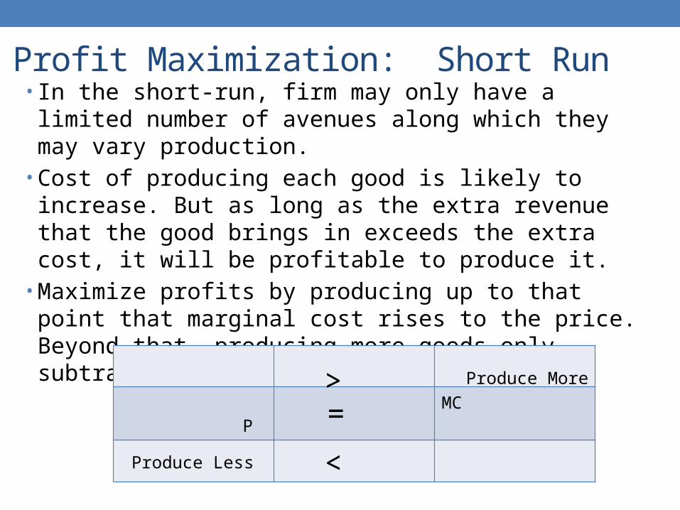
Profit Maximization: Short Run• In the short-run, firm may only have a limited number of
avenues along which they may vary production. • Cost of producing each good is likely to increase. But as long
as the extra revenue that the good brings in exceeds the extra cost, it will be profitable to produce it.
• Maximize profits by producing up to that point that marginal cost rises to the price. Beyond that, producing more goods only subtracts from profits.
P MC=Produce More
<Produce Less
>
Revenues
Costs
Profits
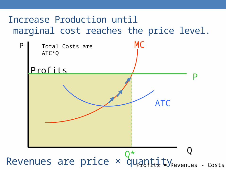
Revenues are price × quantity Q
P
ATC
MC
P
Q*
Increase Production until marginal cost reaches the price level.
Profits = Revenues - Costs
Total Costs are ATC*Q
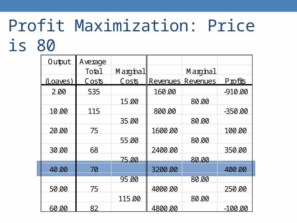
Profit Maximization: Price is 80Output Average
Total Marginal Marginal(Loaves) Costs Costs Revenues Revenues Profits
2.00 535 160.00 -910.0015.00 80.00
10.00 115 800.00 -350.0035.00 80.00
20.00 75 1600.00 100.0055.00 80.00
30.00 68 2400.00 350.0075.00 80.00
40.00 70 3200.00 400.0095.00 80.00
50.00 75 4000.00 250.00115.00 80.00
60.00 82 4800.00 -100.00
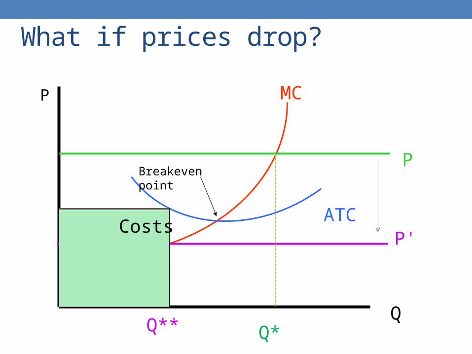
What if prices drop?
Q
P
ATC
MC
P
Q**
-Profits
Revenues
P'
Breakeven point
Q*
Costs
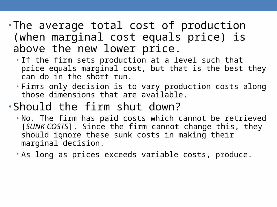
• The average total cost of production (when marginal cost equals price) is above the new lower price. • If the firm sets production at a level such that price equals marginal cost,
but that is the best they can do in the short run. • Firms only decision is to vary production costs along those dimensions
that are available.
• Should the firm shut down?• No. The firm has paid costs which cannot be retrieved [SUNK COSTS].
Since the firm cannot change this, they should ignore these sunk costs in making their marginal decision.
• As long as prices exceeds variable costs, produce.
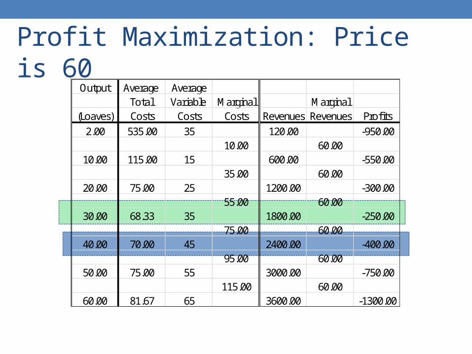
Profit Maximization: Price is 60Output Average Average
Total Variable Marginal Marginal(Loaves) Costs Costs Costs Revenues Revenues Profits
2.00 535.00 35 120.00 -950.0010.00 60.00
10.00 115.00 15 600.00 -550.0035.00 60.00
20.00 75.00 25 1200.00 -300.0055.00 60.00
30.00 68.33 35 1800.00 -250.0075.00 60.00
40.00 70.00 45 2400.00 -400.0095.00 60.00
50.00 75.00 55 3000.00 -750.00115.00 60.00
60.00 81.67 65 3600.00 -1300.00
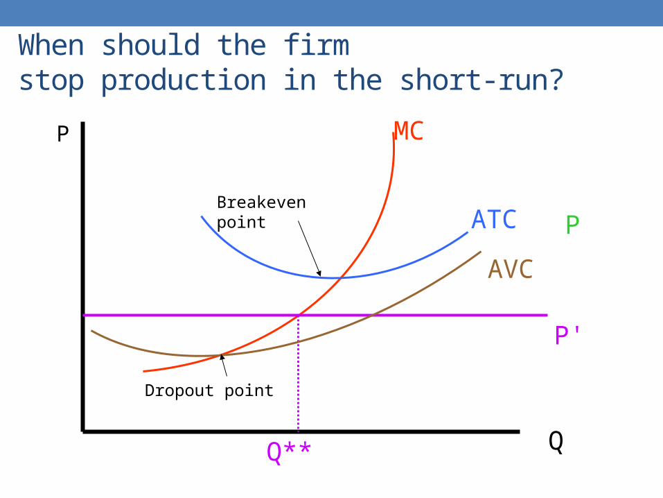
When should the firm stop production in the short-run?
Q
P
ATC
MC
P
Q**
P'
Breakeven point
AVC
Dropout point
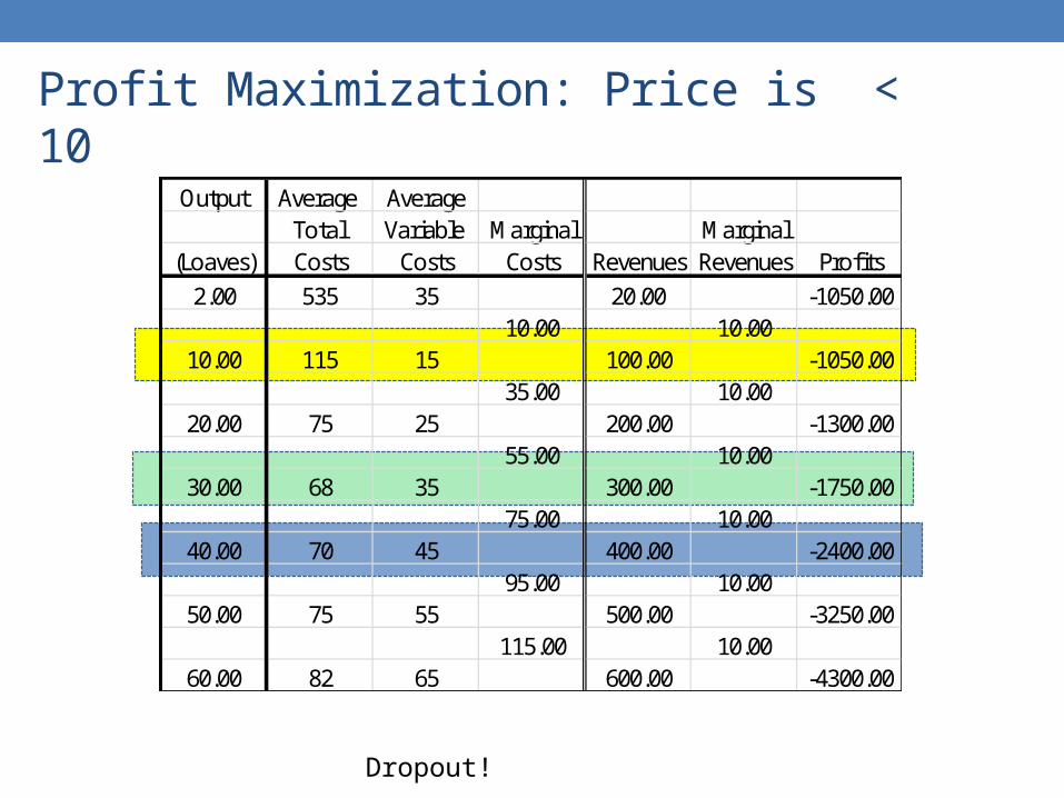
Profit Maximization: Price is < 10Output Average Average
Total Variable Marginal Marginal(Loaves) Costs Costs Costs Revenues Revenues Profits
2.00 535 35 20.00 -1050.0010.00 10.00
10.00 115 15 100.00 -1050.0035.00 10.00
20.00 75 25 200.00 -1300.0055.00 10.00
30.00 68 35 300.00 -1750.0075.00 10.00
40.00 70 45 400.00 -2400.0095.00 10.00
50.00 75 55 500.00 -3250.00115.00 10.00
60.00 82 65 600.00 -4300.00
Dropout!
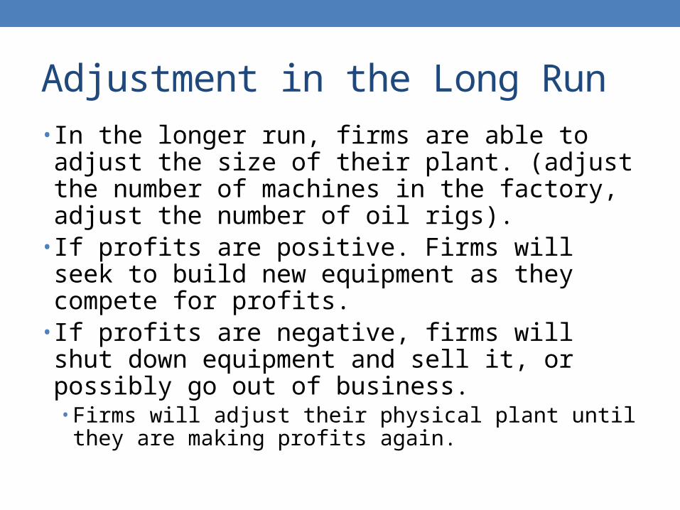
Adjustment in the Long Run• In the longer run, firms are able to adjust the size of their plant. (adjust the number of machines in the factory, adjust the number of oil rigs).
• If profits are positive. Firms will seek to build new equipment as they compete for profits.
• If profits are negative, firms will shut down equipment and sell it, or possibly go out of business.• Firms will adjust their physical plant until they are
making profits again.
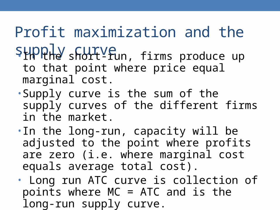
Profit maximization and the supply curve• In the short-run, firms produce up to that point
where price equal marginal cost.• Supply curve is the sum of the supply curves of the different firms in the market.
• In the long-run, capacity will be adjusted to the point where profits are zero (i.e. where marginal cost equals average total cost).
• Long run ATC curve is collection of points where MC = ATC and is the long-run supply curve.
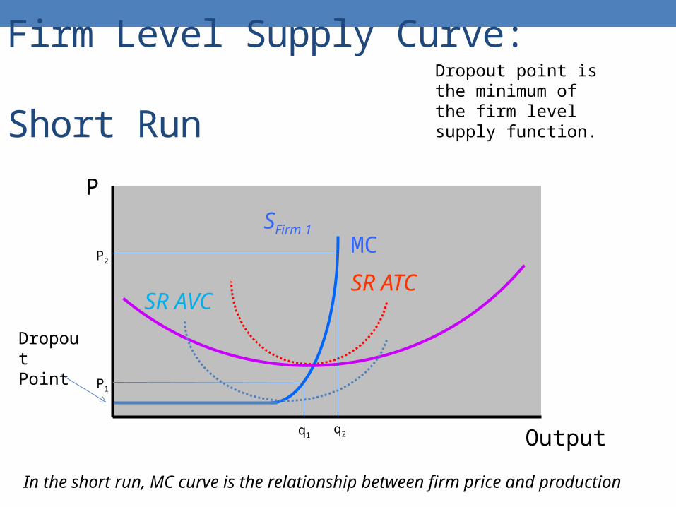
Firm Level Supply Curve: Short Run
Output
SR ATC
MC
P
P1
SFirm 1
In the short run, MC curve is the relationship between firm price and production
q1
P2
q2
DropoutPoint
Dropout point is the minimum of the firm level supply function.
SR AVC
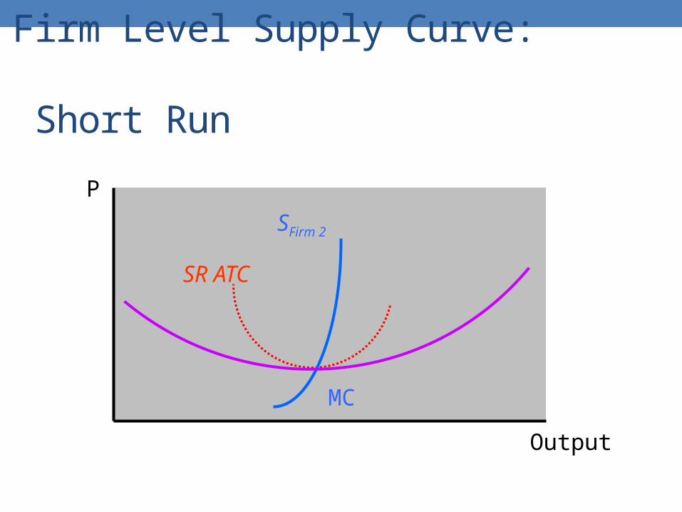
Firm Level Supply Curve: Short Run
Output
SR ATC
MC
P
SFirm 2
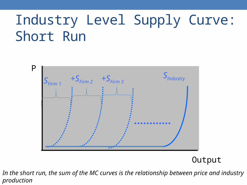
Industry Level Supply Curve:Short Run
Output
P
SFirm 1
In the short run, the sum of the MC curves is the relationship between price and industry production
+SFirm 2 +SFirm 3SIndustry
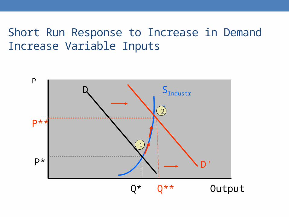
Short Run Response to Increase in DemandIncrease Variable Inputs
SIndustry
Output
PD
Q*
P* D'
Q**
P**
1
2
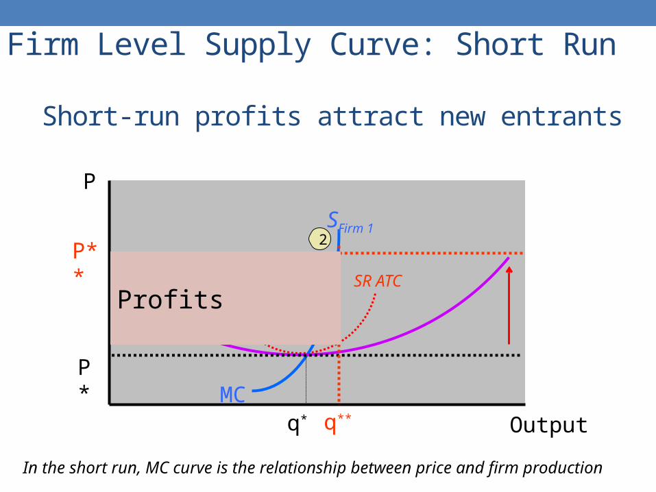
Firm Level Supply Curve: Short Run
Output
SR ATC
MC
P
P*
SFirm 1
In the short run, MC curve is the relationship between price and firm production
P**
q* q**
1
2
Profits
Short-run profits attract new entrants
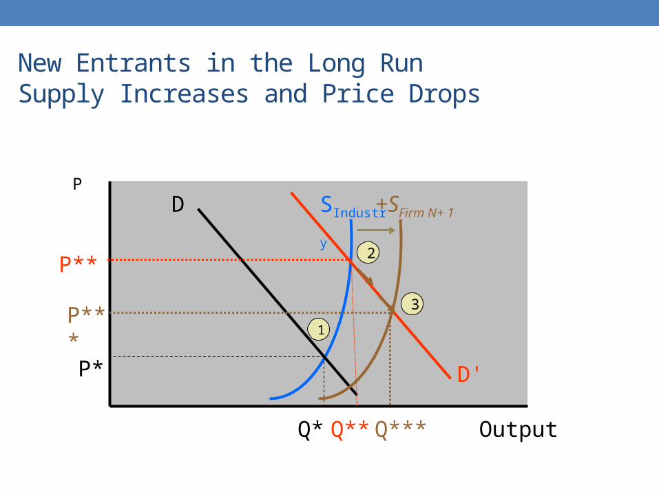
New Entrants in the Long RunSupply Increases and Price Drops
SIndustry
Output
PD
Q*
P* D'
Q**
P**
+SFirm N+ 1
P***
Q***
1
2
3
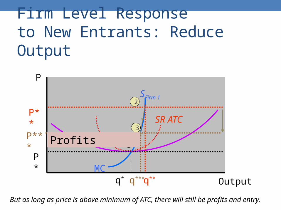
Firm Level Response to New Entrants: Reduce Output
Output
SR ATC
MC
P
P*
SFirm 1
But as long as price is above minimum of ATC, there will still be profits and entry.
P**
q* q**
P***
q***
1
2
3
Profits
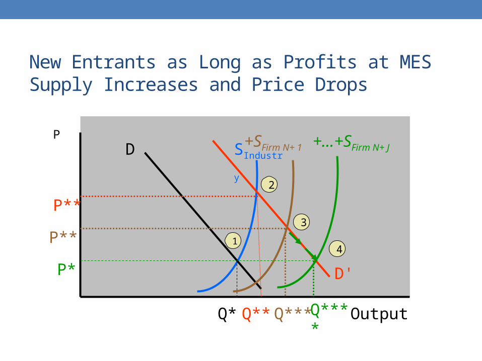
New Entrants as Long as Profits at MESSupply Increases and Price Drops
SIndustry
Output
PD
Q*
P* D'
Q**
P**
+SFirm N+ 1
P**
Q***
+…+SFirm N+ J
Q****
1
2
3
4
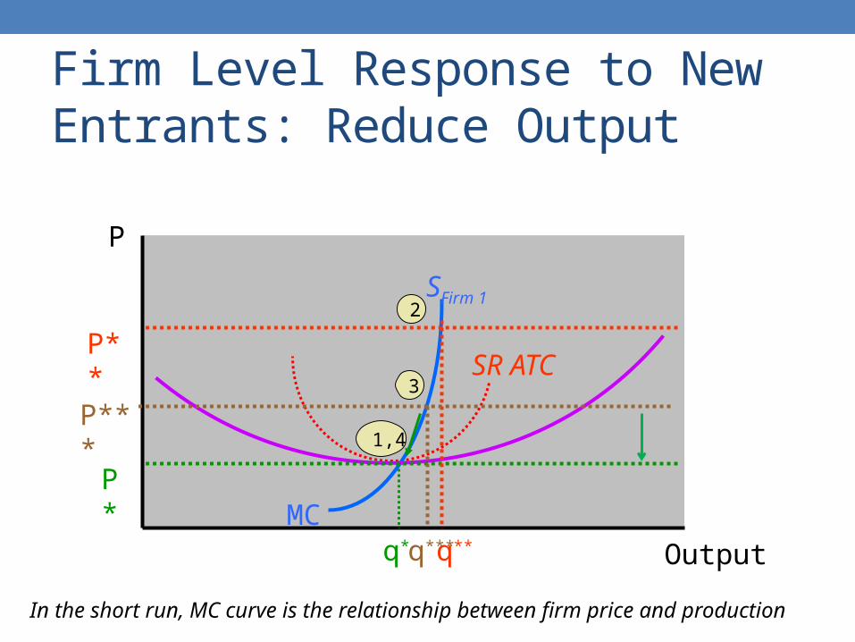
Firm Level Response to New Entrants: Reduce Output
Output
SR ATC
MC
P
P*
SFirm 1
In the short run, MC curve is the relationship between firm price and production
P**
q* q**
P***
q***
1,4
2
3
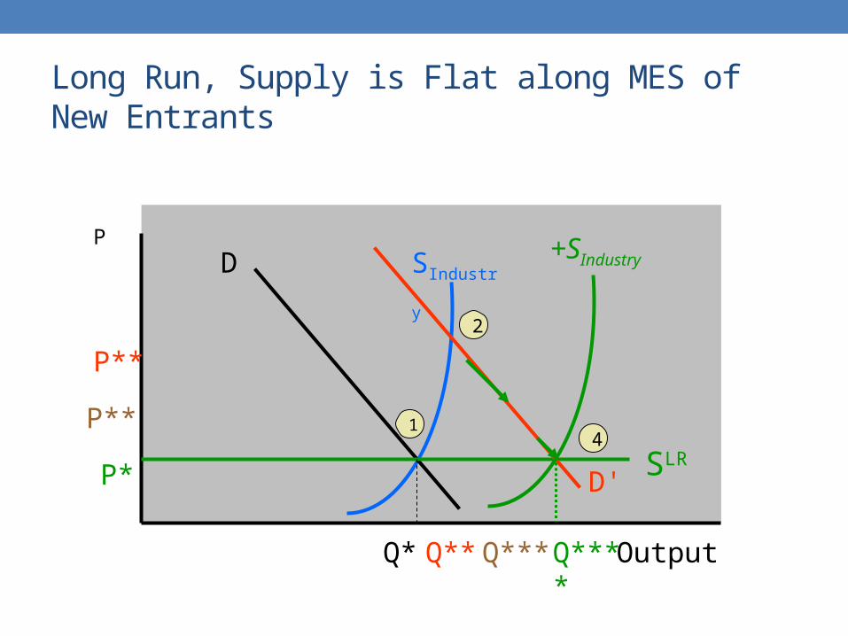
Long Run, Supply is Flat along MES of New Entrants
SIndustry
Output
PD
Q*
P* D'
Q**
P**
P**
Q***
+SIndustry
Q****
SLR
1
2
4
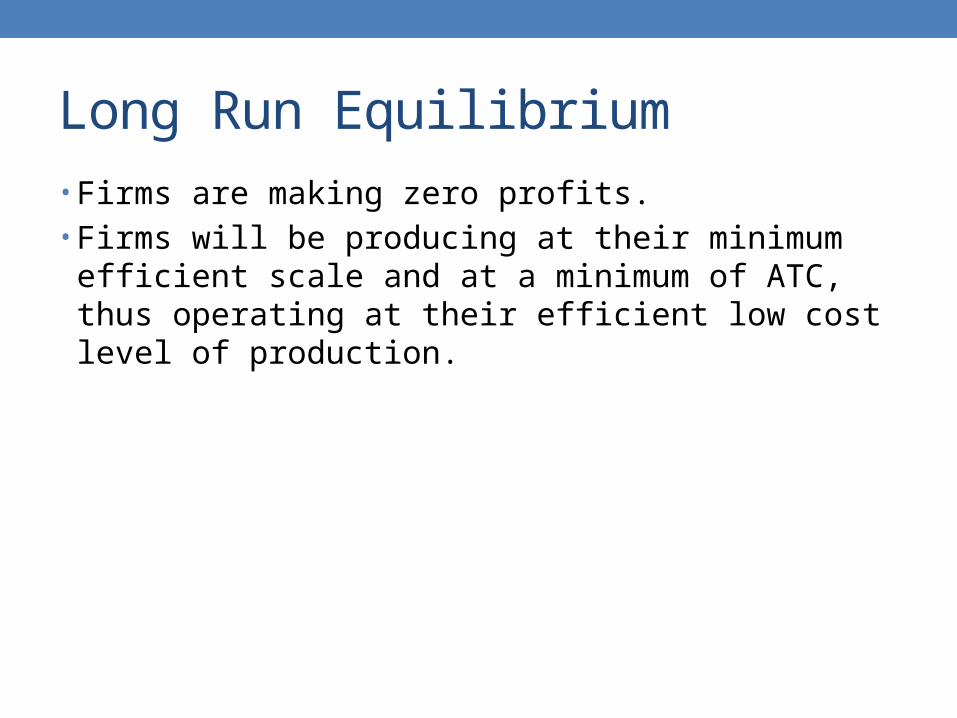
Long Run Equilibrium• Firms are making zero profits.• Firms will be producing at their minimum efficient scale
and at a minimum of ATC, thus operating at their efficient low cost level of production.
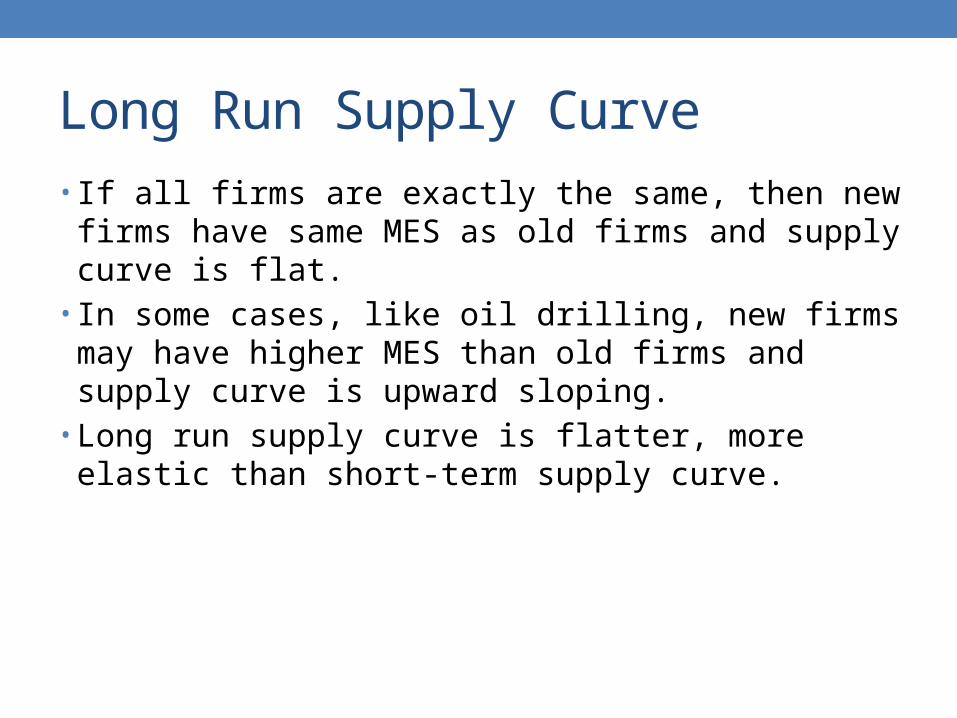
Long Run Supply Curve• If all firms are exactly the same, then new firms have
same MES as old firms and supply curve is flat.• In some cases, like oil drilling, new firms may have higher
MES than old firms and supply curve is upward sloping.• Long run supply curve is flatter, more elastic than short-
term supply curve.
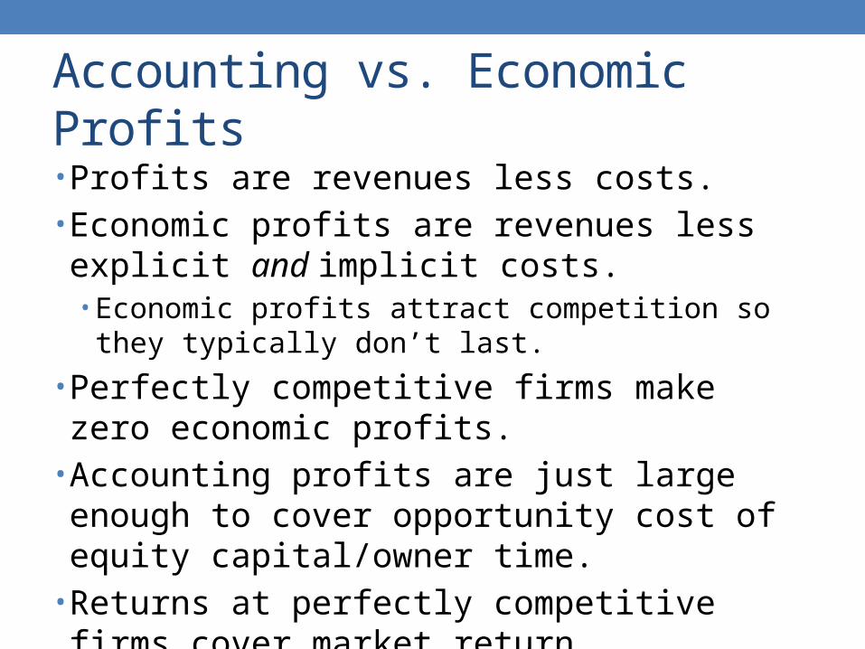
Accounting vs. Economic Profits
• Profits are revenues less costs.• Economic profits are revenues less explicit and implicit costs.• Economic profits attract competition so they typically
don’t last.
• Perfectly competitive firms make zero economic profits.
• Accounting profits are just large enough to cover opportunity cost of equity capital/owner time.
• Returns at perfectly competitive firms cover market return.
MONOPOLYChapter 13
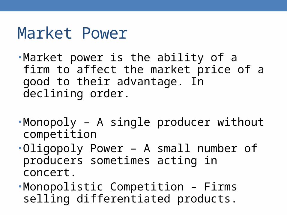
Market Power• Market power is the ability of a firm to affect the market price of a good to their advantage. In declining order.
• Monopoly – A single producer without competition• Oligopoly Power – A small number of producers sometimes acting in concert.
• Monopolistic Competition – Firms selling differentiated products.
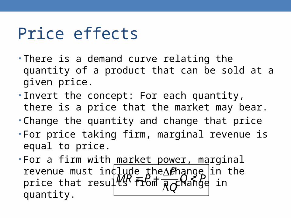
Price effects• There is a demand curve relating the quantity of a product
that can be sold at a given price. • Invert the concept: For each quantity, there is a price that
the market may bear.• Change the quantity and change that price• For price taking firm, marginal revenue is equal to price.• For a firm with market power, marginal revenue must
include the change in the price that results from a change in quantity.
PMR P Q P
Q
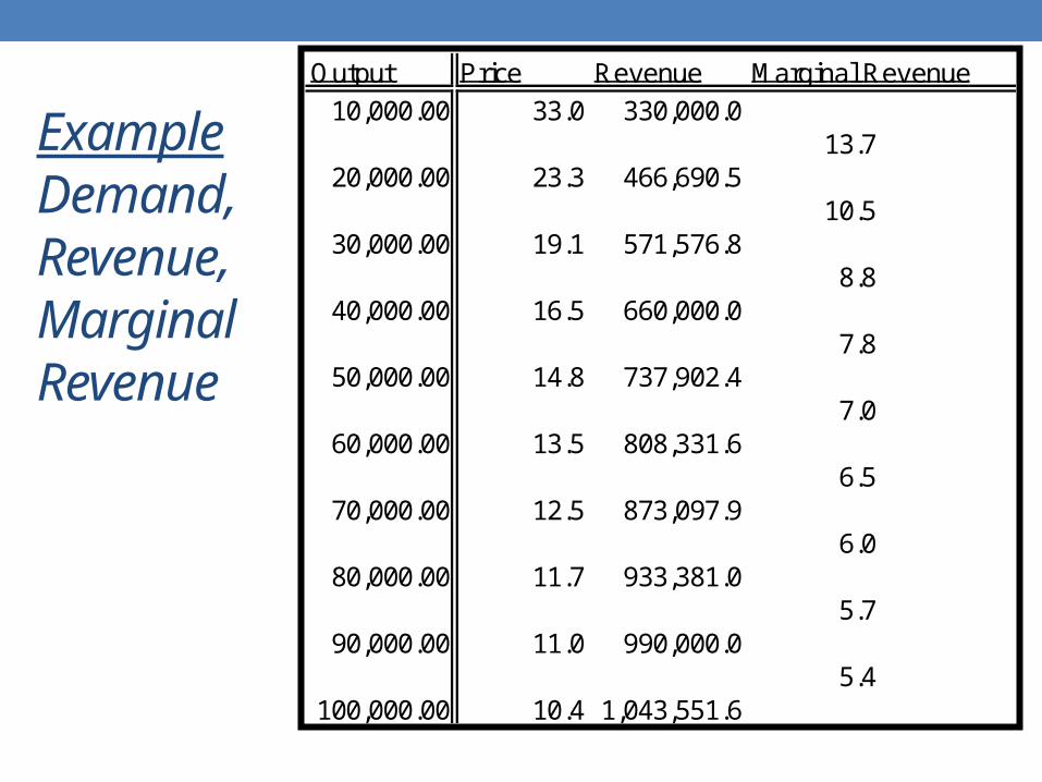
Example Demand, Revenue, Marginal Revenue
Output Price Revenue Marginal Revenue
10,000.00 33.0 330,000.013.7
20,000.00 23.3 466,690.510.5
30,000.00 19.1 571,576.88.8
40,000.00 16.5 660,000.07.8
50,000.00 14.8 737,902.47.0
60,000.00 13.5 808,331.66.5
70,000.00 12.5 873,097.96.0
80,000.00 11.7 933,381.05.7
90,000.00 11.0 990,000.05.4
100,000.00 10.4 1,043,551.6

Example
0.0
5.0
10.0
15.0
20.0
25.0
30.0
35.0
10 20 30 40 50 60 70 80 90
Q
P
Price Marginal Revenue
Demand
MR
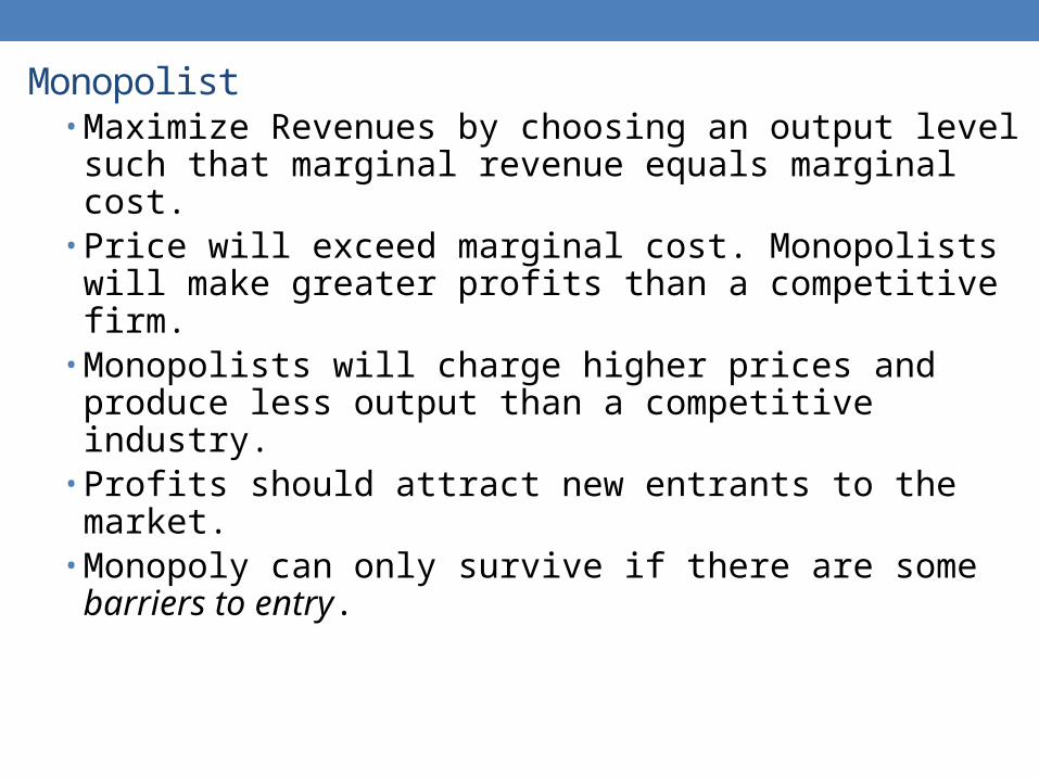
Monopolist• Maximize Revenues by choosing an output level such that
marginal revenue equals marginal cost.• Price will exceed marginal cost. Monopolists will make
greater profits than a competitive firm. • Monopolists will charge higher prices and produce less output
than a competitive industry. • Profits should attract new entrants to the market.• Monopoly can only survive if there are some barriers to entry.
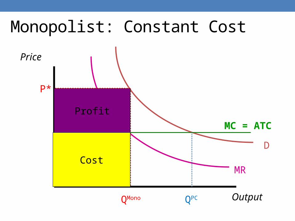
Monopolist: Constant Cost
MC = ATC
MR
D
QMono
P*
QPC
Price
Output
Revenues
Cost
Profit
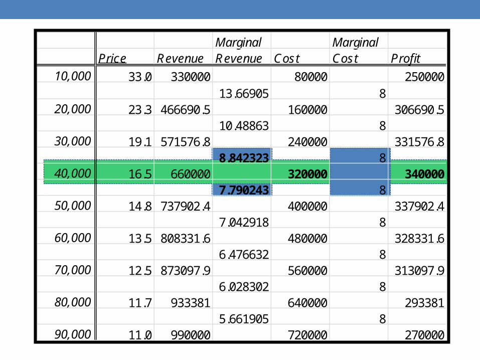
Marginal MarginalPrice Revenue Revenue Cost Cost Profit
10,000 33.0 330000 80000 25000013.66905 8
20,000 23.3 466690.5 160000 306690.510.48863 8
30,000 19.1 571576.8 240000 331576.88.842323 8
40,000 16.5 660000 320000 3400007.790243 8
50,000 14.8 737902.4 400000 337902.47.042918 8
60,000 13.5 808331.6 480000 328331.66.476632 8
70,000 12.5 873097.9 560000 313097.96.028302 8
80,000 11.7 933381 640000 2933815.661905 8
90,000 11.0 990000 720000 270000
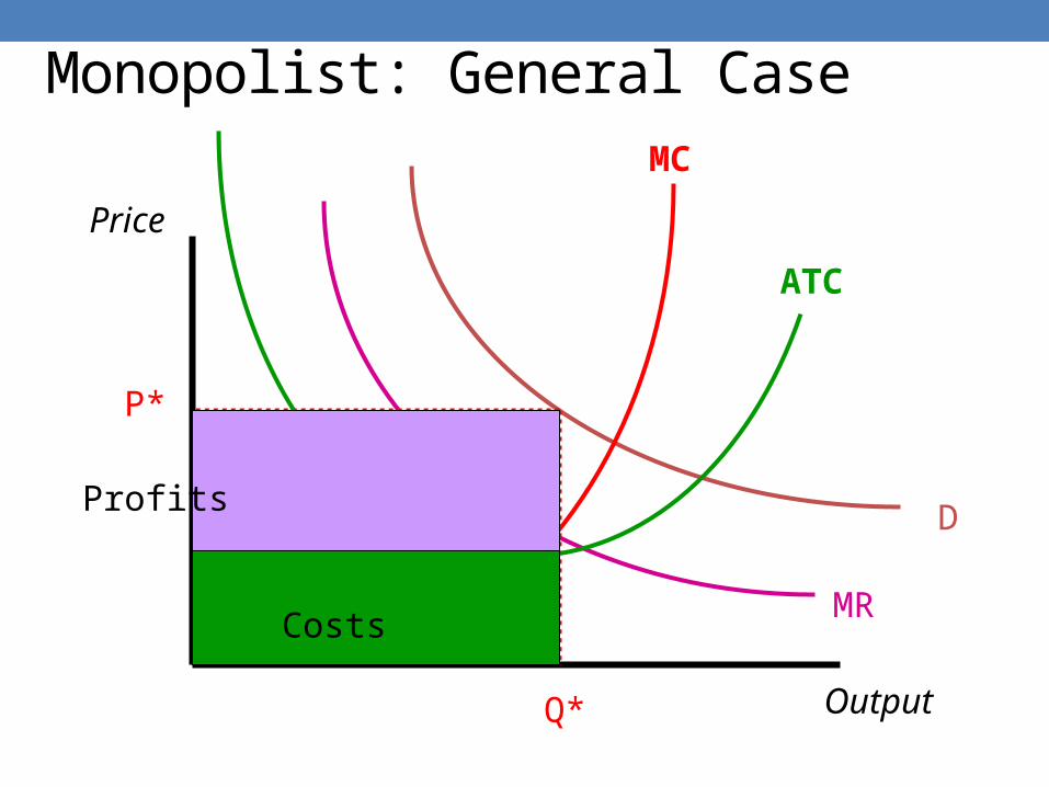
Monopolist: General CaseMC
ATC
MR
D
Q*
P*
Price
Output
Costs
RevenuesProfits
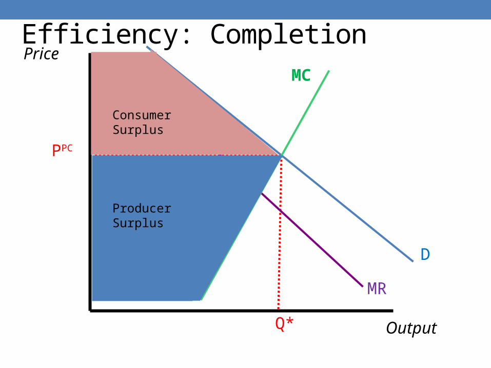
Efficiency: CompletionMC
MR
D
Price
Output
PPC
Q*
Producer Surplus
Consumer Surplus
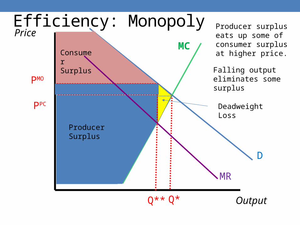
Efficiency: MonopolyMC
MR
D
Price
Output
PPC
Q**
Producer Surplus
Consumer Surplus
Q*
PMO
Producer surplus eats up some of consumer surplus at higher price.
Falling output eliminates some surplus
Deadweight Loss
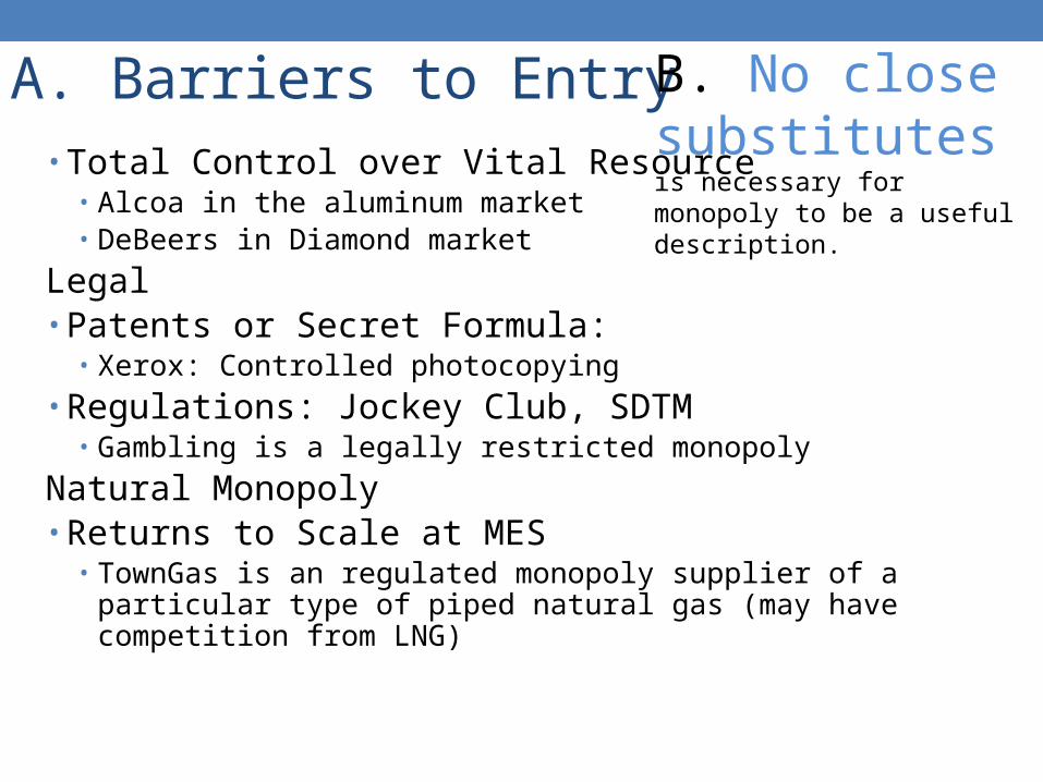
A. Barriers to Entry• Total Control over Vital Resource
• Alcoa in the aluminum market• DeBeers in Diamond market
Legal• Patents or Secret Formula:
• Xerox: Controlled photocopying• Regulations: Jockey Club, SDTM
• Gambling is a legally restricted monopoly
Natural Monopoly• Returns to Scale at MES
• TownGas is an regulated monopoly supplier of a particular type of piped natural gas (may have competition from LNG)
B. No close substitutes is
necessary for monopoly to be a useful description.

Price Discrimination• Demand curve is the price customers are willing to pay. • Some customers are willing to pay a very high price. If
monopolists could tailor a price to each customer they could make maximum profits.
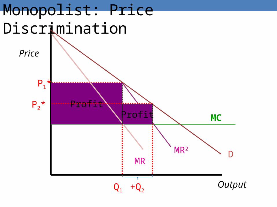
Monopolist: Price Discrimination
MC
MRD
Q1
P1*
Price
Output
Profit
MR2
+Q2
P2*Profit
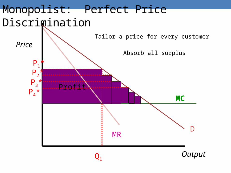
Monopolist: Perfect Price Discrimination
MC
MRD
Q1
P1*
Price
Output
Profit
P2*
Tailor a price for every customer
P3*P4*
Absorb all surplus
Natural Monopoly
• Under certain technologies, there are efficiency gains from concentrating production in a single firm. This occurs if (long-run) costs for a single firm are declining at any production level.
• If firms compete on price, then they will make a loss. ATC is declining when MC<ATC. If firms charge marginal price, they will make a loss and drop out.
• Eventually production involves 1 firm. Firm will naturally exercise market power and earn profits.
• Natural monopoly features technology with large fixed costs.
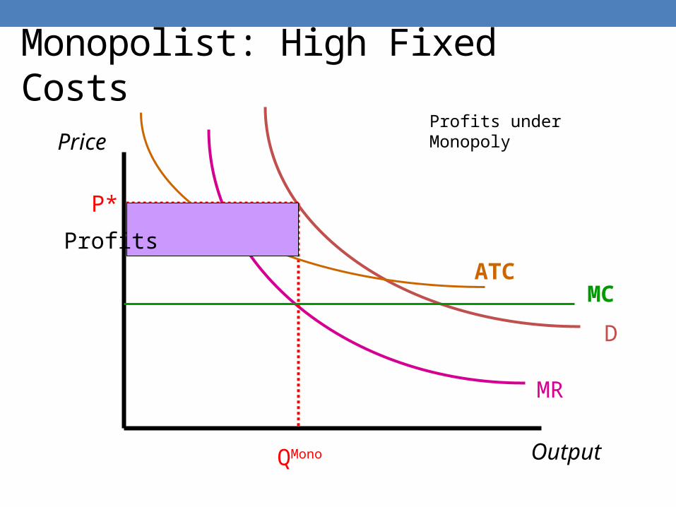
Monopolist: High Fixed Costs
MC
MR
D
QMono
P*
ATC
Price
Output
Profits
Profits under Monopoly
Regulation• Government may step in, usually to put a maximum price level. Should be minimum amount necessary to get the firm to operate small decisions that lead to a competitive outcome.
• Average cost pricing is the lowest price consistent with long-term market participation.
• Information Problem. A single decision maker may not have full access to enough information. Firms have an incentive to overstate costs to regulators.
.
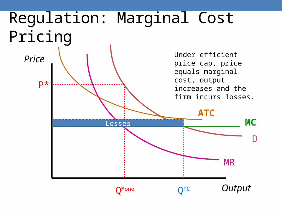
Regulation: Marginal Cost Pricing
MC
MR
D
QMono
P*
QPC
ATC
Price
Output
Under efficient price cap, price equals marginal cost, output increases and the firm incurs losses.
Losses
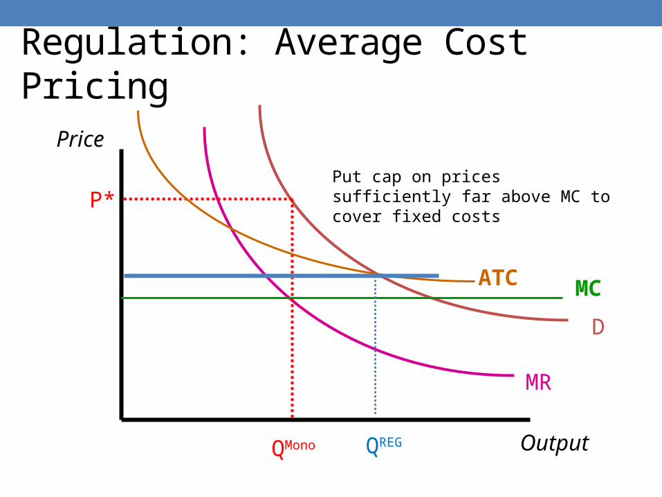
Regulation: Average Cost Pricing
MC
MR
D
QMono
P*
QREG
ATC
Price
Output
Put cap on prices sufficiently far above MC to cover fixed costs
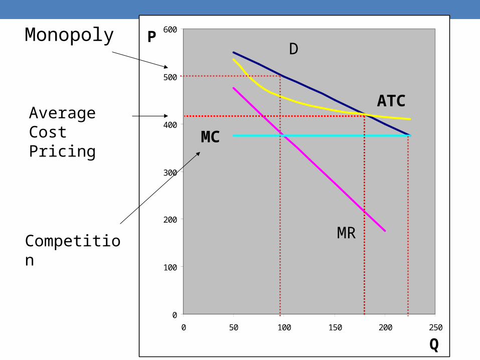
0
100
200
300
400
500
600
0 50 100 150 200 250
Q
P
MC
ATC
MR
DMonopoly
Competition
Average Cost Pricing
MONOPOLISTIC COMPETITIONChapter 14
Monopolistic Competition• Most firms produce a good that is (to a certain extent)
unique. No other good has the exact same properties.• Coke, Pepsi, President’s Choice
• To the extent that you are a unique producer, you will have some market power.
• Price elasticity of individual products are larger than total category. But not infinite as in the case of commodity goods.
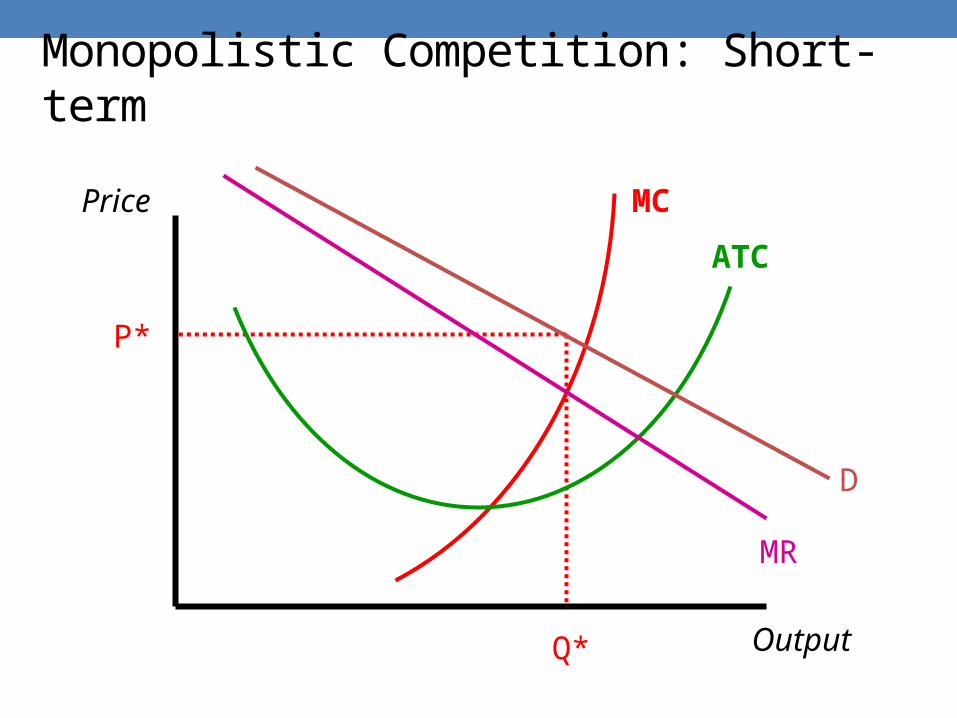
Monopolistic Competition: Short-term
MC
ATC
MR
D
Q*
P*
Price
Output
Characteristics of Monopolistically Competitive Markets• Differentiated Products Download • Free Entry into very similar markets.• Fixed costs of setting up production• Individual firms face downward sloping demand curve and
a falling average total cost curve.• They would sell more if they could at the going rate but lowering
their prices to sell more would lead to losses.
No Barriers to Entry• What happens if new firms can enter?• If there are profits to be had, entrepreneurs will enter
markets to provide close substitutes for profit making goods.
• New goods splitting the market and better substitutes means lower, flatter demand curve.
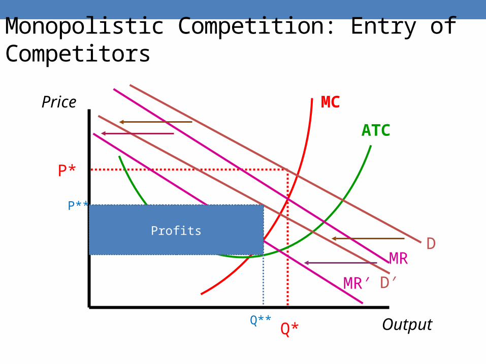
Monopolistic Competition: Entry of Competitors
MC
ATC
MRD
Q*
P*
Price
Output
D′MR′
Q**
P**
Profits
Monopolistic Competition vs. Perfect Competition
• On a market-by-market basis, perfect competition will offer greater efficiency both in terms of minimizing deadweight losses and encouraging an efficient production scale.
• Monopolistic Competition only occurs with differentiated products. • Greater variety generated by this market may compensate for loss
of efficiency.
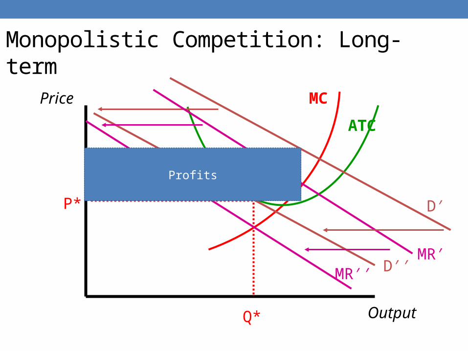
Monopolistic Competition: Long-term
MC
ATC
MR′′ D′′
Q*
P*
Price
Output
D′
MR′
Profits
Monopolistic Competition vs. Perfect Competition
• Similar: Both have many firms, both have zero profits and P = ATC.
• Different: • P > MC : On the margin, monopolistically competitive firms want
more customers. Greater variety generated by this market may compensate for loss of efficiency.
• MC < ATC: Firm is operating at a level that does not minimize total costs.
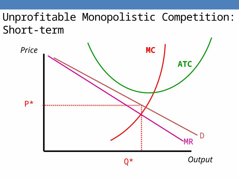
Unprofitable Monopolistic Competition:Short-term
MC
ATC
MRD
Q*
P*
Price
Output
Variety and Monopolistic Competition• Given that most markets have the “feel” of monopolistic
competition, do we have too many firms or is variety it’s own reward?
• Does advertising create phony differentiation or provide information?
Monopolistic Competition and Entrepreneurship
• New markets are frequently developed. • For many goods, the only barriers to entry is imagination. • Entrepreneurs develop new ideas for new goods. The
pay-off for entrepreneurship are short-run monopoly profits. (Ted Turner and CNN). Only in rare cases will firms be able to make long-term monopolistic profits.
Consequences of Market Power• One clear consequence of the existence of market power is
that prices are higher than marginal cost and output is smaller than perfect competition.
• Additional consequences of the presence of market power may be:• Complacency by firms managers (i.e. standard corporate governance
measures do not generate efficiency)• Rent-seeking: Firms may put effort into constructing artificial barriers
to entry rather than producing goods.
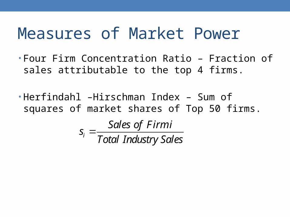
Measures of Market Power• Four Firm Concentration Ratio – Fraction of sales
attributable to the top 4 firms.
• Herfindahl –Hirschman Index – Sum of squares of market shares of Top 50 firms.
i
Sales of Firm is
Total Industry Sales
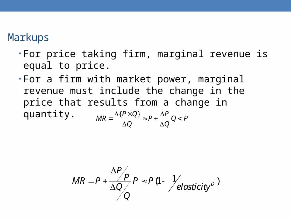
Markups• For price taking firm, marginal revenue is equal to price.• For a firm with market power, marginal revenue must
include the change in the price that results from a change in quantity.
{ }P Q PMR P Q P
Q Q
1(1 )D
PPMR P P P
Q elasticityQ
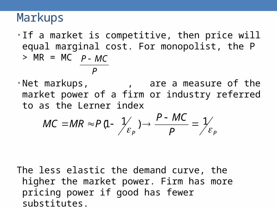
Markups• If a market is competitive, then price will equal marginal
cost. For monopolist, the P > MR = MC
• Net markups, , are a measure of the market power of a firm or industry referred to as the Lerner index
The less elastic the demand curve, the higher the market power. Firm has more pricing power if good has fewer substitutes.
1 1(1 )P P
P MCMC MR P
P
P MC
P
Learning OutcomesStudents should be able to • Characterize a perfectly competitive market.• Calculate total revenue, marginal revenue and profit for a firm in a competitive market.
• Describe the supply curve in a competitive market in both the short and long run.
• Characterize the relationship between price, marginal revenue, marginal cost, average total cost, and profits in a monopolistic market.
• Measure the degree of market power with the Lerner index.
• Describe 4 barriers to entry that may enable monopoly power.