INDUSTRIAL STATISTICS AND OPERATIONAL MANAGEMENT

4 : ASSIGNMENT PROBLEM

Dr. Ravi Mahendra Gor Associate Dean

ICFAI Business School ICFAI House,

Nr. GNFC INFO Tower S. G. Road Bodakdev

Ahmedabad-380054

Ph.: 079-26858632 (O); 079-26464029 (R); 09825323243 (M) E-mail: ravigor@hotmail.com

IntroductionMathematical formulation of APSome theoremsSolution methods of AP

Enumeration method Simplex method Transportation method The Hungarian method

Variations of the APMultiple optimal solution Unbalanced AP Problem with infeasible (restricted) assignment Maximization case in AP

Review Exercise

CHAPTER 4

ASSIGNMENT PROBLEM

4.1 Introduction :

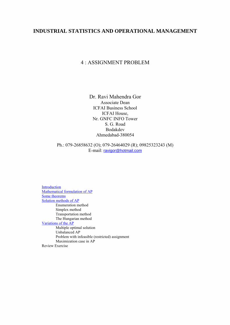
Consider the following situation:

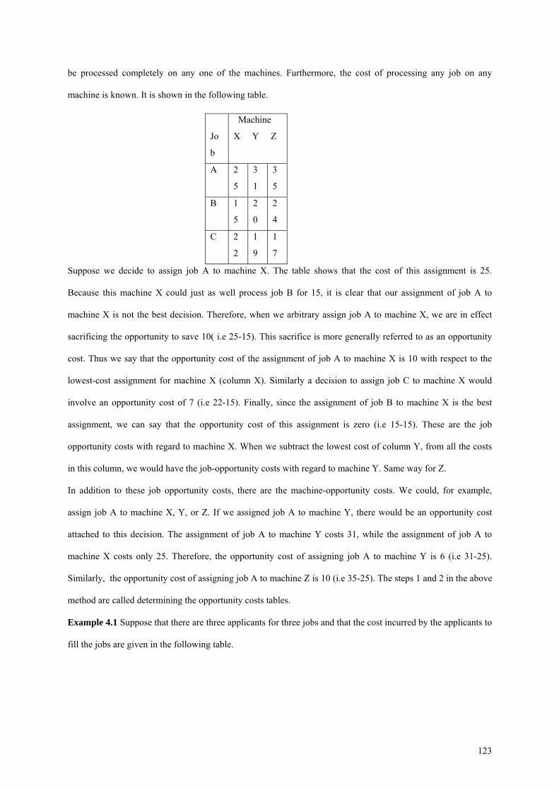
A company does custom metalworking for a number of local plants. It currently has three jobs say A,

B and C to be done. It also has three machines say X, Y and Z on which to do the work. Any one of the jobs can

be processed completely on any one of the machines. Furthermore, the cost of processing any job on any

machine is known. It is shown in the following table.

Job

Machine

X Y Z

A 25 31 35

B 15 20 24

C 22 19 17

The assignment of jobs to machines must be on one-to-one basis; that is, each job must be assigned exclusively

to one and only one machine. The objective is to assign the jobs to the machines so as to minimize total cost.

The assignment problem (AP) is a particular sub - class of the transportation problem. It can be stated

in the general form as follows: Given n - facilities, n - jobs and the effectiveness of each facility for each job,

the problem is to assign each facility to one and only one job in such a way that the measure of the effectiveness

is optimized (maximized or minimized). Here the facilities represent sources and the jobs represent the

destinations or sinks in the transportation ‘language’.

Associated to each assignment problem there is a matrix called the cost or effectiveness matrix [cij]

where cij is the cost or measure of effectiveness of assigning ith job to the jth facility. An assignment plan is

optimal if it also minimizes (optimizes) the total cost or effectiveness of doing all the jobs.

Distribute m - units (jobs) (one available at each of the origin J1, J2, ..., Jm) to the m - destination

requiring only 1 unit (job) in a way which minimizes the total cost. We can see that the problem is similar to the

transportation problem.

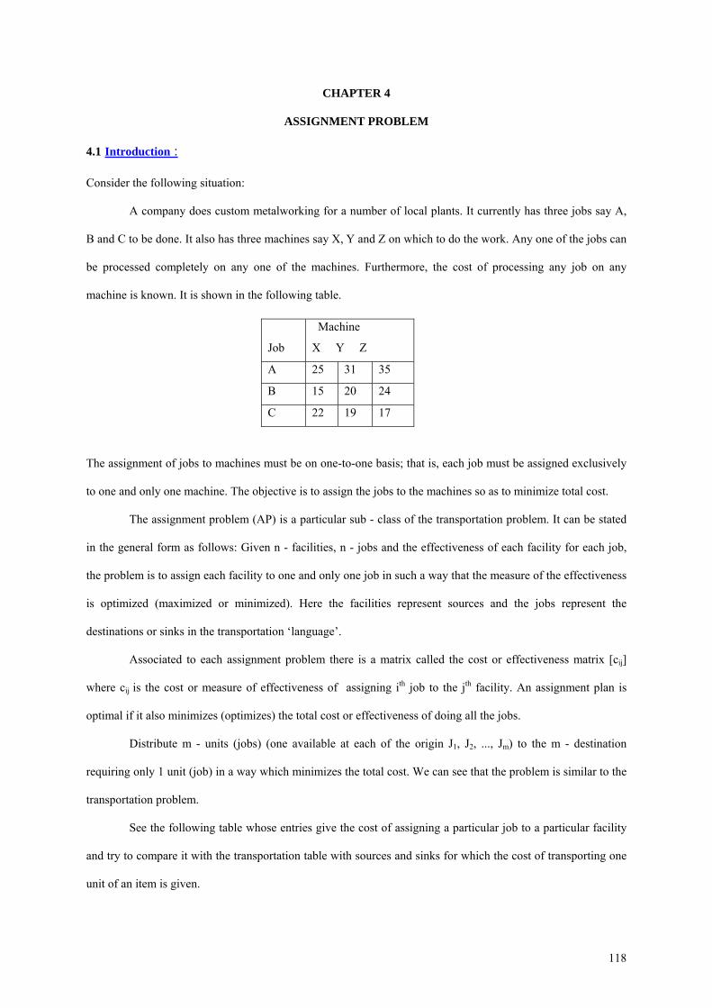
See the following table whose entries give the cost of assigning a particular job to a particular facility

and try to compare it with the transportation table with sources and sinks for which the cost of transporting one

unit of an item is given.

118

Facilities ( destinations)

F1 F2 F3 . . Fm ai

J1 C11 C12 C13 . . C1m 1

J2 C21 C22 C23 . . C2m 1

. . . . . . . .

. . . . . . . .

Jm Cm1 Cm2 Cm3 . . Cmm 1

Job

s

bj 1 1 1 1

The only difference between standard assignment and a transportation problem is that here always number of

origins is equal to the number of destinations and at each origin always one unit is available and always one unit

is required at each destination. Here, the cost matrix is always square. Thus, each job can be assigned to only

one facility.

4.2 Mathematical formulation of the AP :

Let xij = ⎧⎨1, if i - th job is assigned to j - th facility0, if i - th job is not assigned to j - th facility⎩

Determine xij , i, j = 1, 2, ..., m so as to

Minimize (4.1) m m

1 1

subject to , j = 1, 2, ..., m (4.2)

, i = 1, 2, ..., m (4.3)

z c xij iji j=

= =

iji =

ij

∑ ∑

1x =∑1

m

1xj

=∑1

m

=

and xij = 0 or 1 (4.4)

The condition (4.4) is similar to the condition (3.4) of a transportation problem which states that xij ≥ 0.

We can see that the assignment problem is thus a special case of a transportation problem where m = n and ai =

bj = 1. Due to this similarity with the transportation problem, we can handle AP by transportation technique

also.

119

It may however be easily observed that any basic feasible solution of an AP contains (2m - 1) - variables out

of which (m - 1) - variables are zero. Due to this high degree of degeneracy the computational techniques given

in Chapter 3 of a TP become very inefficient. A separate computational method is required to solve AP.

The basic principles on which the solution of an AP is based can be stated as the following two

theorems :

4.3 Some Theorems :

Theorem 4.3.1 : If a constant is added to every element of a row and / or column of the cost matrix of an AP,

the resulting AP has the same optimal solution as the original problem and vice versa. Alternatively, if xij = xij*

minimizes

x over all1 1

ij such that m m

, xij ≥ 0 then

z c xij iji j= ∑ ∑

= =

= =11 1

m mx xij iji j

∑ ∑= =

xij = xij* also minimizes where cij

* = cij ± ui ± vj , for i, j = 1, 2, ..., m and ui , vj * *1 1

m mz c xij iji j

= ∑ ∑= =

are real numbers.

* *1 1

m mz c xij iji j

= ∑ ∑= =

Proof :

Now and are added / subtracted from z to give z* are independent of xij . Therefore, z* is

minimum when z is minimum. Hence, xij = xij* also minimizes z*.

1

mu∑ v j∑ii = j =

±∑ ∑= =

( )1 1

m mc u v xij i j iji j

= ±

1 1 1 1 1 1

m m m m m mc x u x v xij ij i ij j iji j i j i j

= ± ±∑ ∑ ∑ ∑ ∑ ∑= = = = = =

1 1 1 1

m m m mz u x v xi ij j ijj i

= ± ±∑ ∑ ∑ ∑= = = =i j

11 1 1 1

m m m mz u v x xi j ij iji j i j

= ± ± = =∑ ∑ ∑ ∑= = = =

Q

1

m

120

Theorem 4.3.2 : If all cij ≥ 0 and we have obtained a solution with xij = xij* such that

, then the present solution is an optimal solution * 0c xij ij =∑ ∑1 1

m m

Proof : As neither of the cij is negative, the value of cannot be negative. Hence its minimum

value is zero which is attained at xij = xij*. Hence, the present solution is optimal.

i j= =

1 1

m mz c xij iji j= ∑ ∑

= =

4.4 Solution methods of AP :

An assignment problem can be solved by following four methods out of which the Hungarian method

is more suitable for solving the assignment problems.

• Enumeration method

• Simplex method

• Transportation problem

• Hungarian method.

4.4.1 Enumeration method : It may be noted that with n - facilities and n - jobs there are n ! possible

assignments. One way of finding an optimum assignment is to write all n ! possible arrangements, evaluate their

total cost (in terms of the given measure of effectiveness) and select the assignment with minimum cost. The

method leads to a computational problem of formidable size even when the value of n is moderate. Even for n =

10, the possible number of arrangements is 3628800.

4.4.2 Simplex method : An assignment problem can be solved by simplex method after converting it into zero -

one integer programming problem. But as there would be n × n - decision variables and 2n (i.e. n + n) -

equalities, it is again difficult to solve it manually.

4.4.3 Transportation method : Article 4.2 clearly depicts why an assignment problem should not be solved by

the transportation method.

4.4.4 The Hungarian method : The Hungarian method was developed by H. Kuhn and is based upon the work

of two Hungarian mathematicians; D. Konig and J. Egervary. For application of the algorithm, it is assumed

that all of the cij’s of the starting cost matrix are non-negative integers and the assignment problem is of

minimization case.

Algorithm for the Hungarian method :

121

Step 1 : Subtract the minimum of each row of the effectiveness matrix, from all the elements of the respective

rows.

Step 2 : Further, modify the resulting matrix by subtracting the minimum element of each column from all the

elements of the column.

Step 3 : Draw, the minimum number of horizontal and vertical lines to suppress all the zeros. Let the number of

lines drawn be N.

(i) If N = n (n = number of rows or columns), optimal assignment can be made. Hence go to step 6.

(ii) If N < n, go to step 4.

Step 4 : Find the smallest uncovered element ( that is not covered by the lines drawn). Subtract it from all

uncovered entries. Add it to all entries on the intersection of the two lines.

Step 5 : Repeat Step 3 and Step 4 until N = n.

Step 6 : Find a row with exactly one 0 entry. Encircle it by □ . Cancel that column and row showing that the

zeroes in that column cannot be taken for further assignment. Continue this process until all rows are examined.

Repeat it for columns also. This step is called zero assigning.

Step 7 : Continue Step 6 until

(i) no unmarked zero is left.

(ii) there lies more than one of the unmarked zeroes in the column or row.

In case (i) the procedure terminates. In case (ii), mark □ one of the unmarked zeroes arbitrarily and

cancel the remaining zeroes in its row and column. Repeat the process until no unmarked zero is left in the

matrix.

Step 8 : Exactly one marked □ zero in each row and each column is obtained. The assignment corresponding

to these marked □ zeroes will give the optimum assignment.

This method is also known as Flood’s technique or Reduced Matrix Method.

Significance of the step 1 and step 2 in the Hungarain algorithm:

The assignment algorithm applies the concept of opportunity costs. The cost of any kind of action or decision

consists of the opportunities that are sacrificed in taking that action. If we do one thing, we cannot do another.

Let us take the example given at the start of the chapter.

A company does custom metalworking for a number of local plants. It currently has three jobs say A,

B and C to be done. It also has three machines say X, Y and Z on which to do the work. Any one of the jobs can

122

be processed completely on any one of the machines. Furthermore, the cost of processing any job on any

machine is known. It is shown in the following table.

Suppose we decide to assign job A to machine X. The table shows that the cost of this assignment is 25.

Because this machine X could just as well process job B for 15, it is clear that our assignment of job A to

machine X is not the best decision. Therefore, when we arbitrary assign job A to machine X, we are in effect

sacrificing the opportunity to save 10( i.e 25-15). This sacrifice is more generally referred to as an opportunity

cost. Thus we say that the opportunity cost of the assignment of job A to machine X is 10 with respect to the

lowest-cost assignment for machine X (column X). Similarly a decision to assign job C to machine X would

involve an opportunity cost of 7 (i.e 22-15). Finally, since the assignment of job B to machine X is the best

assignment, we can say that the opportunity cost of this assignment is zero (i.e 15-15). These are the job

opportunity costs with regard to machine X. When we subtract the lowest cost of column Y, from all the costs

in this column, we would have the job-opportunity costs with regard to machine Y. Same way for Z.

Jo

b

Machine

X Y Z

A 2

5

3

1

3

5

B 1

5

2

0

2

4

C 2

2

1

9

1

7

In addition to these job opportunity costs, there are the machine-opportunity costs. We could, for example,

assign job A to machine X, Y, or Z. If we assigned job A to machine Y, there would be an opportunity cost

attached to this decision. The assignment of job A to machine Y costs 31, while the assignment of job A to

machine X costs only 25. Therefore, the opportunity cost of assigning job A to machine Y is 6 (i.e 31-25).

Similarly, the opportunity cost of assigning job A to machine Z is 10 (i.e 35-25). The steps 1 and 2 in the above

method are called determining the opportunity costs tables.

Example 4.1 Suppose that there are three applicants for three jobs and that the cost incurred by the applicants to

fill the jobs are given in the following table.

123

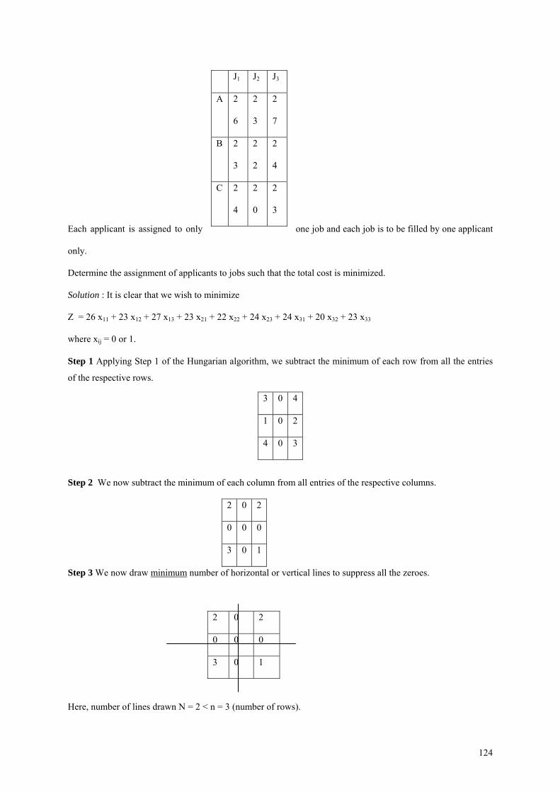
Each applicant is assigned to only one job and each job is to be filled by one applicant

only.

J1 J2 J3

A 2

6

2

3

2

7

B 2

3

2

2

2

4

C 2

4

2

0

2

3

Determine the assignment of applicants to jobs such that the total cost is minimized.

Solution : It is clear that we wish to minimize

Z = 26 x11 + 23 x12 + 27 x13 + 23 x21 + 22 x22 + 24 x23 + 24 x31 + 20 x32 + 23 x33

where xij = 0 or 1.

Step 1 Applying Step 1 of the Hungarian algorithm, we subtract the minimum of each row from all the entries

of the respective rows.

Step 2 We now subtract the minimum of each column from all entries of the respective columns.

2 0 2

0 0 0

3 0 1

Step 3 We now draw minimum number of horizontal or vertical lines to suppress all the zeroes.

2 0 2

0 0 0

3 0 1

3 0 4

1 0 2

4 0 3

Here, number of lines drawn N = 2 < n = 3 (number of rows).

124

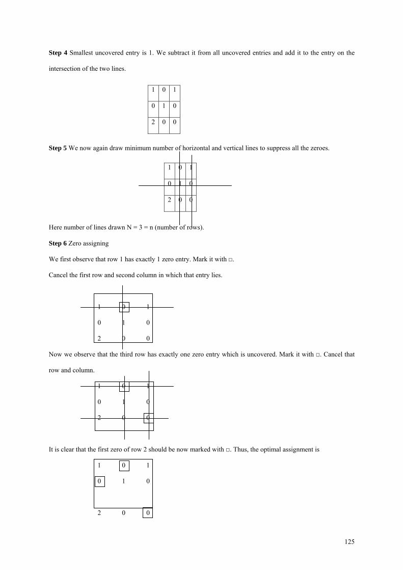
Step 4 Smallest uncovered entry is 1. We subtract it from all uncovered entries and add it to the entry on the

intersection of the two lines.

1 0 1

0 1 0

2 0 0

Step 5 We now again draw minimum number of horizontal and vertical lines to suppress all the zeroes.

Here number of lines drawn N = 3 = n (number of rows).

Step 6 Zero assigning

We first observe that row 1 has exactly 1 zero entry. Mark it with □.

Cancel the first row and second column in which that entry lies.

1 0 1

0 1 0

2 0 0

Now we observe that the third row has exactly one zero entry which is uncovered. Mark it with □. Cancel that

row and column.

1 0 1

0 1 0

2 0 0

It is clear that the first zero of row 2 should be now marked with □. Thus, the optimal assignment is

1 0 1

0 1 0

2 0 0

1 0 1

0 1 0

2 0 0

125

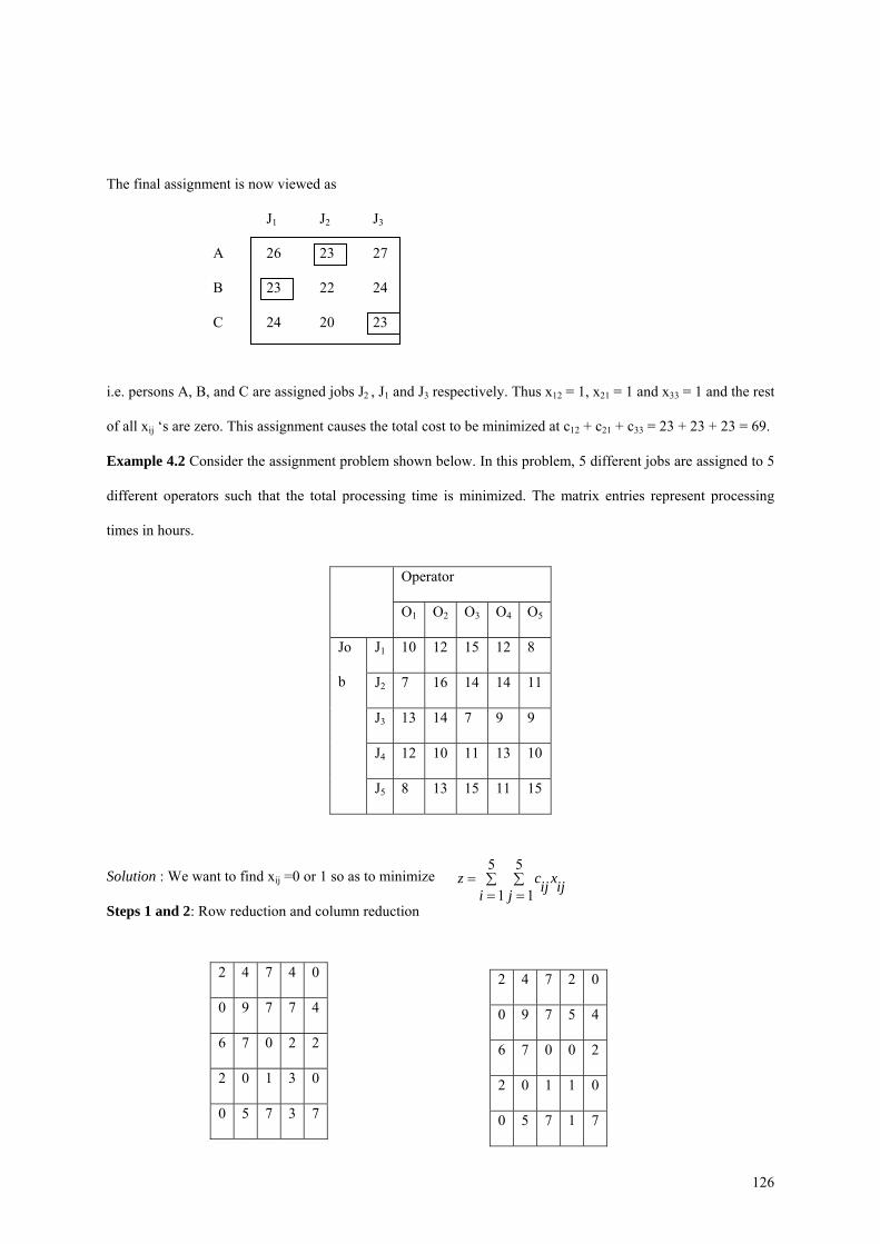
The final assignment is now viewed as

J1 J2 J3

A 26 23 27

B 23 22 24

C 24 20 23

i.e. persons A, B, and C are assigned jobs J2 , J1 and J3 respectively. Thus x12 = 1, x21 = 1 and x33 = 1 and the rest

of all xij ‘s are zero. This assignment causes the total cost to be minimized at c12 + c21 + c33 = 23 + 23 + 23 = 69.

Example 4.2 Consider the assignment problem shown below. In this problem, 5 different jobs are assigned to 5

different operators such that the total processing time is minimized. The matrix entries represent processing

times in hours.

Operator

O1 O2 O3 O4 O5

J1 10 12 15 12 8

J2 7 16 14 14 11

J3 13 14 7 9 9

J4 12 10 11 13 10

Jo

b

J5 8 13 15 11 15

5 5

1 1z c xij iji j= ∑ ∑

= =Solution : We want to find xij =0 or 1 so as to minimize

Steps 1 and 2: Row reduction and column reduction

2 4 7 4 0

0 9 7 7 4

6 7 0 2 2

2 0 1 3 0

0 5 7 3 7

2 4 7 2 0

0 9 7 5 4

6 7 0 0 2

2 0 1 1 0

0 5 7 1 7

126

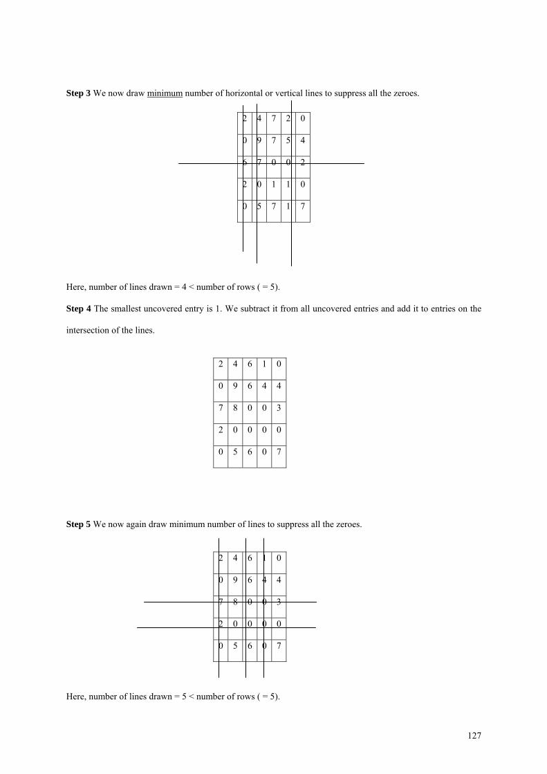
Step 3 We now draw minimum number of horizontal or vertical lines to suppress all the zeroes.

Here, number of lines drawn = 4 < number of rows ( = 5).

Step 4 The smallest uncovered entry is 1. We subtract it from all uncovered entries and add it to entries on the

intersection of the lines.

Step 5 We now again draw minimum number of lines to suppress all the zeroes.

2 4 7 2 0

0 9 7 5 4

6 7 0 0 2

2 0 1 1 0

0 5 7 1 7

2 4 6 1 0

0 9 6 4 4

7 8 0 0 3

2 0 0 0 0

0 5 6 0 7

2 4 6 1 0

0 9 6 4 4

7 8 0 0 3

2 0 0 0 0

0 5 6 0 7

Here, number of lines drawn = 5 < number of rows ( = 5).

127

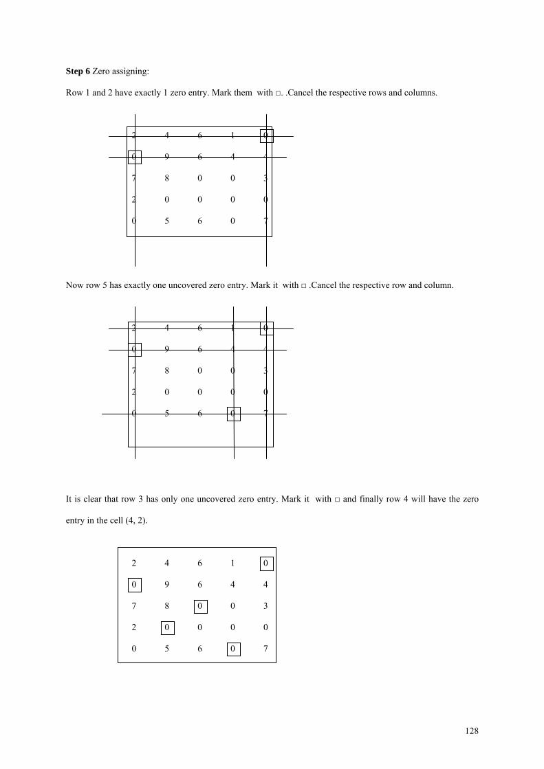
Step 6 Zero assigning:

Row 1 and 2 have exactly 1 zero entry. Mark them with □. .Cancel the respective rows and columns.

2 4 6 1 0

0 9 6 4 4

7 8 0 0 3

2 0 0 0 0

0 5 6 0 7

Now row 5 has exactly one uncovered zero entry. Mark it with □ .Cancel the respective row and column.

2 4 6 1 0

0 9 6 4 4

7 8 0 0 3

2 0 0 0 0

0 5 6 0 7

It is clear that row 3 has only one uncovered zero entry. Mark it with □ and finally row 4 will have the zero

entry in the cell (4, 2).

2 4 6 1 0

0 9 6 4 4

7 8 0 0 3

2 0 0 0 0

0 5 6 0 7

128

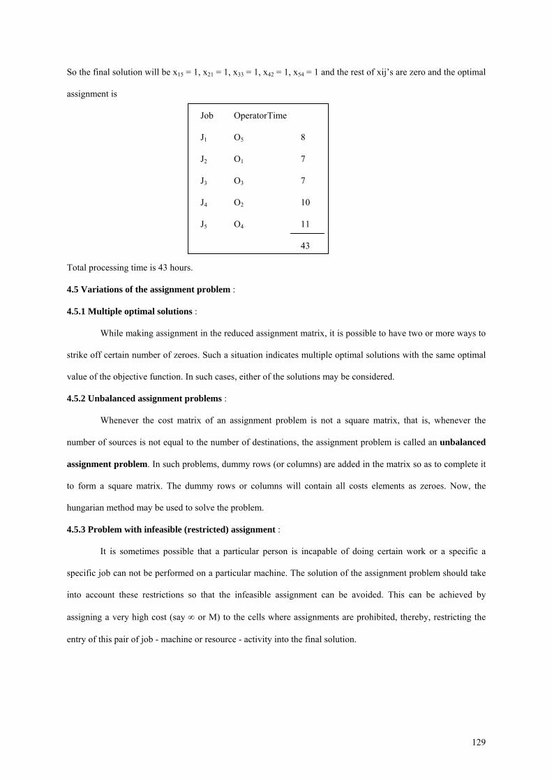
So the final solution will be x15 = 1, x21 = 1, x33 = 1, x42 = 1, x54 = 1 and the rest of xij’s are zero and the optimal

assignment is

Job Operator Time

J1 O5 8

J2 O1 7

J3 O3 7

J4 O2 10

J5 O4 11

43

Total processing time is 43 hours.

4.5 Variations of the assignment problem :

4.5.1 Multiple optimal solutions :

While making assignment in the reduced assignment matrix, it is possible to have two or more ways to

strike off certain number of zeroes. Such a situation indicates multiple optimal solutions with the same optimal

value of the objective function. In such cases, either of the solutions may be considered.

4.5.2 Unbalanced assignment problems :

Whenever the cost matrix of an assignment problem is not a square matrix, that is, whenever the

number of sources is not equal to the number of destinations, the assignment problem is called an unbalanced

assignment problem. In such problems, dummy rows (or columns) are added in the matrix so as to complete it

to form a square matrix. The dummy rows or columns will contain all costs elements as zeroes. Now, the

hungarian method may be used to solve the problem.

4.5.3 Problem with infeasible (restricted) assignment :

It is sometimes possible that a particular person is incapable of doing certain work or a specific a

specific job can not be performed on a particular machine. The solution of the assignment problem should take

into account these restrictions so that the infeasible assignment can be avoided. This can be achieved by

assigning a very high cost (say ∞ or M) to the cells where assignments are prohibited, thereby, restricting the

entry of this pair of job - machine or resource - activity into the final solution.

129

4.5.4 Maximization case in assignment problems :

There are problems where certain facilities have to be assigned to a number of jobs so as to maximize

the overall performance of the assignment. The problem can be converted into a minimization problem in the

following two ways and then Hungarian method can be used for its solution.

Method 1 : Select the greatest element of the given cost matrix and then subtract each element of the matrix

from the greatest element to get the modified matrix.

Note that the new matrix will be [cij*] where cij

* = crk - cij where crk is the greatest element and [cij] is

the original cost matrix.

Now (say) xij = xij* maximizes .

1 1

m mz c xij iji j= ∑ ∑

= = Then

* *1 1

m mz c xij iji j

= ∑ ∑= =

( )1 1

m mc c xrk ij iji j

= −∑ ∑= =

1 1 1 1

m m m mc x c xrk ij ij iji j i j

= −∑ ∑ ∑ ∑= = = =

1 1

m mc x zrk iji j

= −∑ ∑= =

So if xij = xij* maximizes z, it also minimizes z*.

Method 2 : Multiply each element of the matrix by (- 1) to get the modified matrix. Note that in this case the

new matrix is [cij*] where cij

* = (- cij ). So if

xij = xij* maximizes . Then

1 1

m m* ( )

1 1

m mz c xij iji j= −∑ ∑

= =z c xij iji j= ∑ ∑

= =

Thus, xij = xij* minimizes z*.

Example 4.3 Five different machines can do any of the required five jobs with different profits resulting from

each assignment as given below.

130

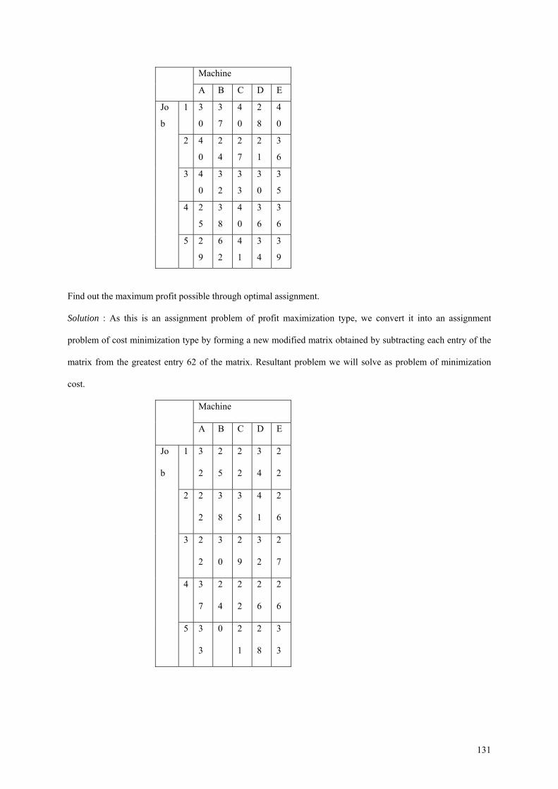
Machine

A B C D E

1 3

0

3

7

4

0

2

8

4

0

2 4

0

2

4

2

7

2

1

3

6

3 4

0

3

2

3

3

3

0

3

5

4 2

5

3

8

4

0

3

6

3

6

Jo

b

5 2

9

6

2

4

1

3

4

3

9

Find out the maximum profit possible through optimal assignment.

Solution : As this is an assignment problem of profit maximization type, we convert it into an assignment

problem of cost minimization type by forming a new modified matrix obtained by subtracting each entry of the

matrix from the greatest entry 62 of the matrix. Resultant problem we will solve as problem of minimization

cost.

Machine

A B C D E

1 3

2

2

5

2

2

3

4

2

2

2 2

2

3

8

3

5

4

1

2

6

3 2

2

3

0

2

9

3

2

2

7

4 3

7

2

4

2

2

2

6

2

6

Jo

b

5 3

3

0 2

1

2

8

3

3

131

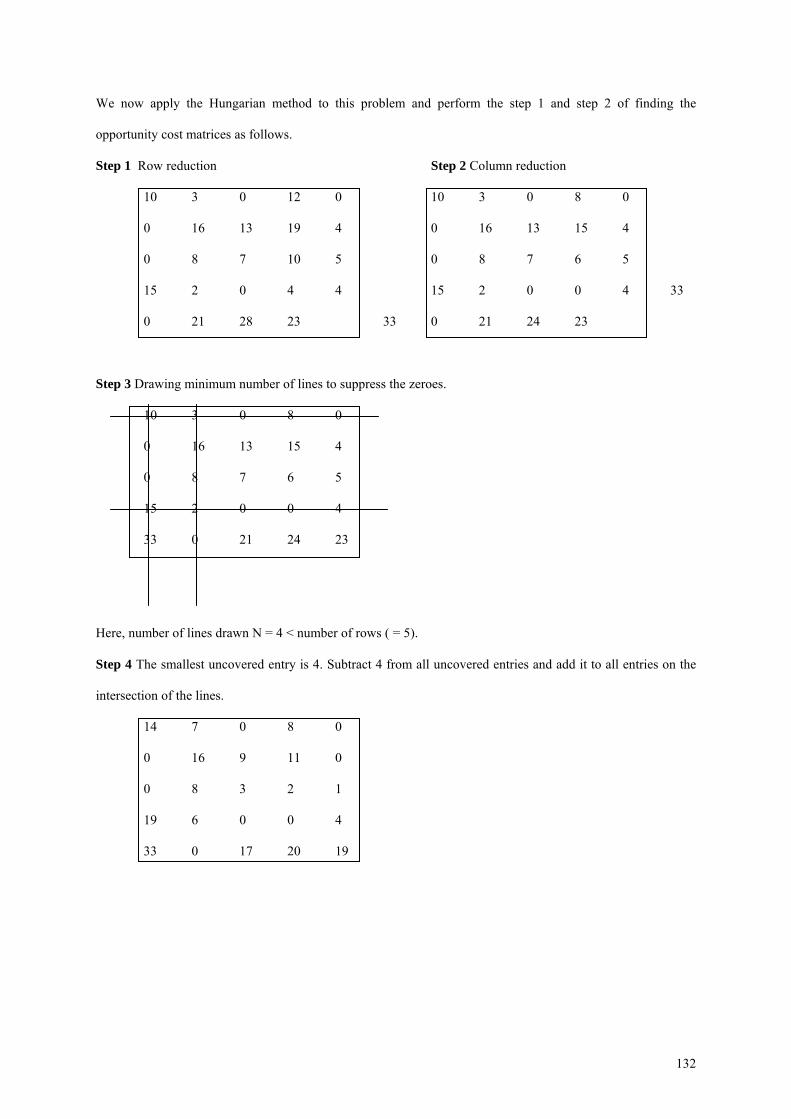
We now apply the Hungarian method to this problem and perform the step 1 and step 2 of finding the

opportunity cost matrices as follows.

Step 1 Row reduction Step 2 Column reduction

10 3 0 12 0 10 3 0 8 0

0 16 13 19 4 0 16 13 15 4

0 8 7 10 5 0 8 7 6 5

15 2 0 4 4 15 2 0 0 4 33

0 21 28 23 33 0 21 24 23

Step 3 Drawing minimum number of lines to suppress the zeroes.

10 3 0 8 0

0 16 13 15 4

0 8 7 6 5

15 2 0 0 4

33 0 21 24 23

Here, number of lines drawn N = 4 < number of rows ( = 5).

Step 4 The smallest uncovered entry is 4. Subtract 4 from all uncovered entries and add it to all entries on the

intersection of the lines.

14 7 0 8 0

0 16 9 11 0

0 8 3 2 1

19 6 0 0 4

33 0 17 20 19

132

Step 5 Draw minimum number of lines to cover all the zeroes.

14 7 0 8 0

0 16 9 11 0

0 8 3 2 1

19 6 0 0 4

33 0 17 20 19

Here the number of lines drawn N = 5 = number of rows.

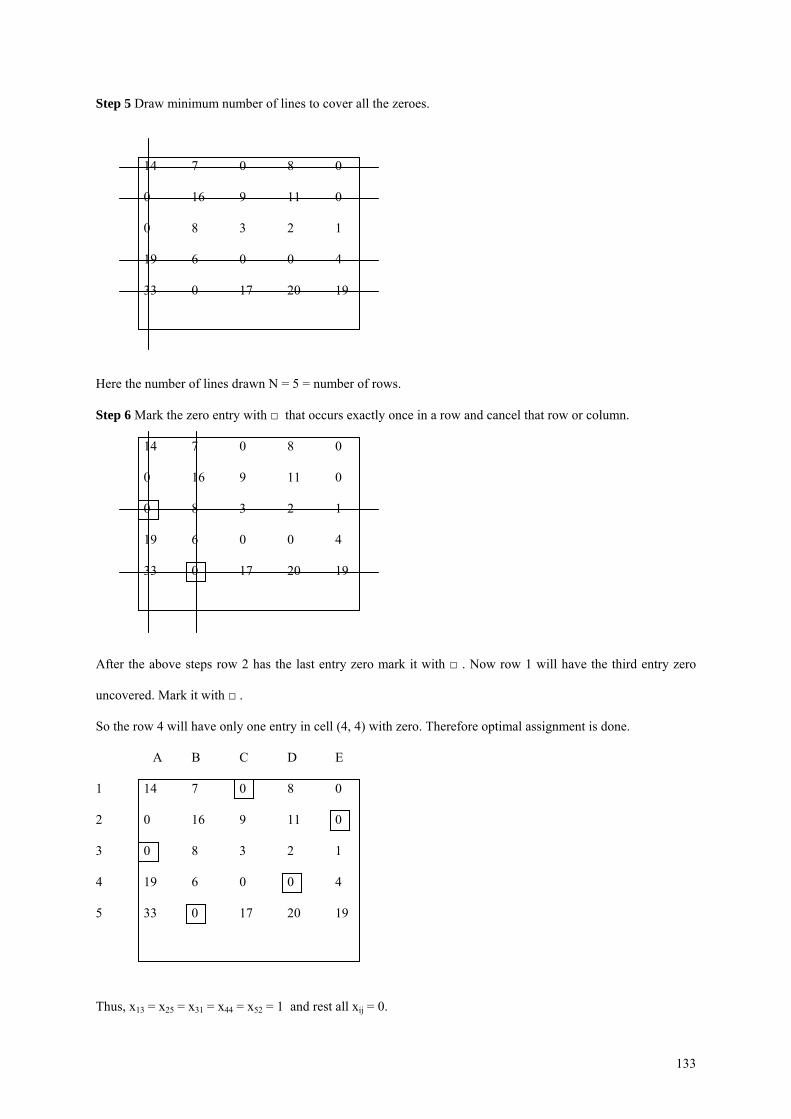
Step 6 Mark the zero entry with □ that occurs exactly once in a row and cancel that row or column.

14 7 0 8 0

0 16 9 11 0

0 8 3 2 1

19 6 0 0 4

33 0 17 20 19

After the above steps row 2 has the last entry zero mark it with □ . Now row 1 will have the third entry zero

uncovered. Mark it with □ .

So the row 4 will have only one entry in cell (4, 4) with zero. Therefore optimal assignment is done.

A B C D E

1 14 7 0 8 0

2 0 16 9 11 0

3 0 8 3 2 1

4 19 6 0 0 4

5 33 0 17 20 19

Thus, x13 = x25 = x31 = x44 = x52 = 1 and rest all xij = 0.

133

The optimal assignment is

Job Machine Profit

1 C 40

2 E 36

3 A 40

4 D 36

5 B 62

214

Therefore, maximum profit is 214.

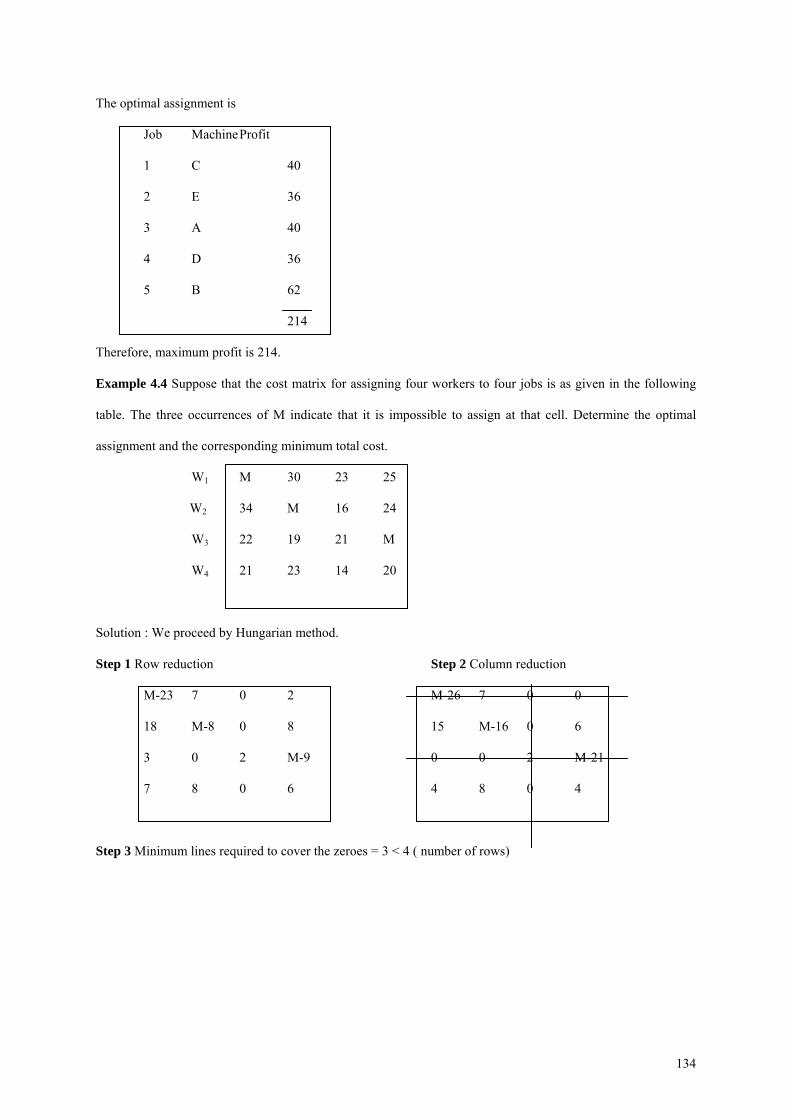
Example 4.4 Suppose that the cost matrix for assigning four workers to four jobs is as given in the following

table. The three occurrences of M indicate that it is impossible to assign at that cell. Determine the optimal

assignment and the corresponding minimum total cost.

W1 M 30 23 25

W2 34 M 16 24

W3 22 19 21 M

W4 21 23 14 20

Solution : We proceed by Hungarian method.

Step 1 Row reduction Step 2 Column reduction

M-23 7 0 2 M-26 7 0 0

18 M-8 0 8 15 M-16 0 6

3 0 2 M-9 0 0 2 M-21

7 8 0 6 4 8 0 4

Step 3 Minimum lines required to cover the zeroes = 3 < 4 ( number of rows)

134

Step 4

M-26 7 4 0

11 M-20 0 2

0 0 6 M-21

0 5 0 0

Step 5 As the number of lines required to cover all zeroes = 4 = (number of rows). The optimal assignment can

be made. (left for the reader to fill details)

Worker Job Total cost

W1 J4 25

W2 J3 16

W3 J2 19

W4 J1 21

81

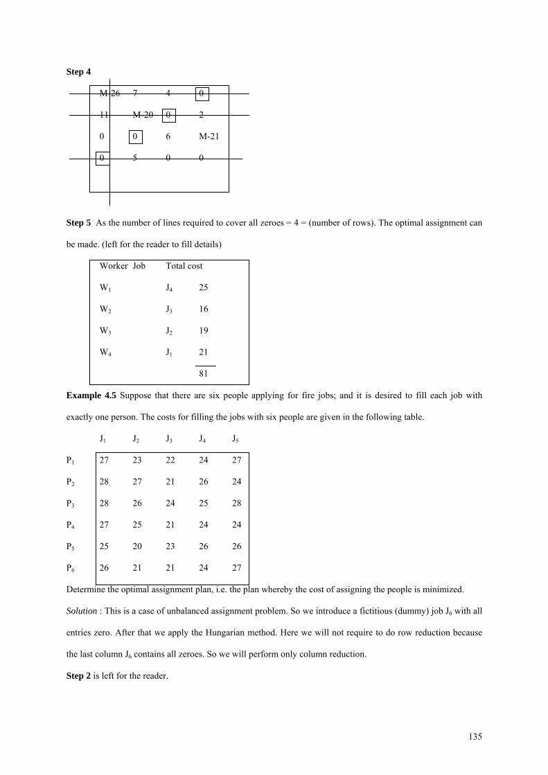
Example 4.5 Suppose that there are six people applying for fire jobs; and it is desired to fill each job with

exactly one person. The costs for filling the jobs with six people are given in the following table.

J1 J2 J3 J4 J5

P1 27 23 22 24 27

P2 28 27 21 26 24

P3 28 26 24 25 28

P4 27 25 21 24 24

P5 25 20 23 26 26

P6 26 21 21 24 27

Determine the optimal assignment plan, i.e. the plan whereby the cost of assigning the people is minimized.

Solution : This is a case of unbalanced assignment problem. So we introduce a fictitious (dummy) job J6 with all

entries zero. After that we apply the Hungarian method. Here we will not require to do row reduction because

the last column J6 contains all zeroes. So we will perform only column reduction.

Step 2 is left for the reader.

135

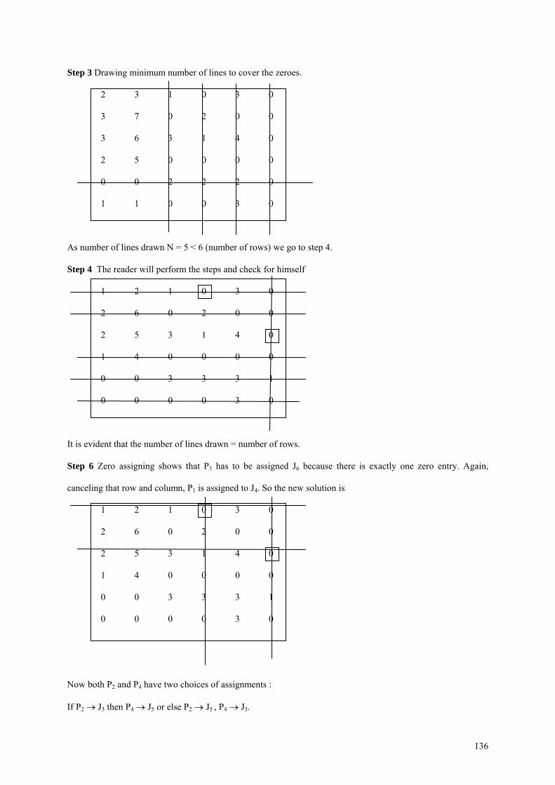
Step 3 Drawing minimum number of lines to cover the zeroes.

2 3 1 0 3 0

3 7 0 2 0 0

3 6 3 1 4 0

2 5 0 0 0 0

0 0 2 2 2 0

1 1 0 0 3 0

As number of lines drawn N = 5 < 6 (number of rows) we go to step 4.

Step 4 The reader will perform the steps and check for himself

1 2 1 0 3 0

2 6 0 2 0 0

2 5 3 1 4 0

1 4 0 0 0 0

0 0 3 3 3 1

0 0 0 0 3 0

It is evident that the number of lines drawn = number of rows.

Step 6 Zero assigning shows that P3 has to be assigned J6 because there is exactly one zero entry. Again,

canceling that row and column, P1 is assigned to J4. So the new solution is

1 2 1 0 3 0

2 6 0 2 0 0

2 5 3 1 4 0

1 4 0 0 0 0

0 0 3 3 3 1

0 0 0 0 3 0

Now both P2 and P4 have two choices of assignments :

If P2 → J3 then P4 → J5 or else P2 → J5 , P4 → J3.

136

Again if P5 → J1 then P6 → J2 or else P5 → J2 , P5 → J1.

So this is a case of alternative optimal solution.

Solution 1 Solution 2

Person Job Cost Person Job Cost

P1 J4 24 P1 J4 24

P2 J3 21 P2 J5 24

P3 J6 0 P3 J6 0

P4 J5 24 P4 J3 21

P5 J1 25 P5 J2 20

P6 J2 21 P6 J1 26

115 115

Here, it may be noted that P3 → J6 means P3 is not assigned to any job J1 to J5.

REVIEW EXERCISE

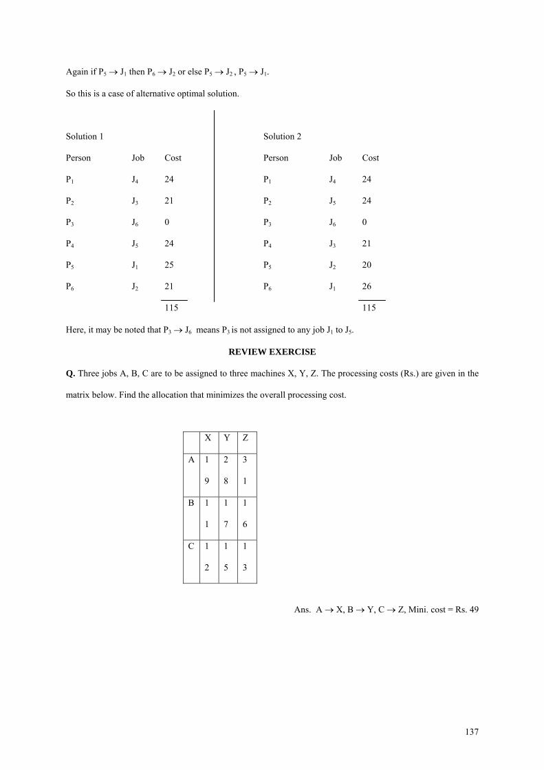
Q. Three jobs A, B, C are to be assigned to three machines X, Y, Z. The processing costs (Rs.) are given in the

matrix below. Find the allocation that minimizes the overall processing cost.

X Y Z

A 1

9

2

8

3

1

B 1

1

1

7

1

6

C 1

2

1

5

1

3

Ans. A → X, B → Y, C → Z, Mini. cost = Rs. 49

137

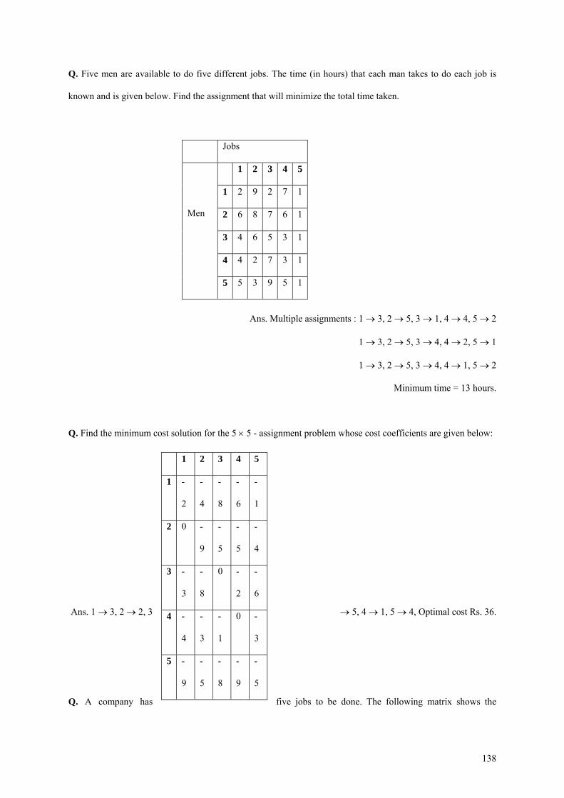
Q. Five men are available to do five different jobs. The time (in hours) that each man takes to do each job is

known and is given below. Find the assignment that will minimize the total time taken.

Jobs

1 2 3 4 5

1 2 9 2 7 1

2 6 8 7 6 1

3 4 6 5 3 1

4 4 2 7 3 1

Men

5 5 3 9 5 1

Ans. Multiple assignments : 1 → 3, 2 → 5, 3 → 1, 4 → 4, 5 → 2

1 → 3, 2 → 5, 3 → 4, 4 → 2, 5 → 1

1 → 3, 2 → 5, 3 → 4, 4 → 1, 5 → 2

Minimum time = 13 hours.

Q. Find the minimum cost solution for the 5 × 5 - assignment problem whose cost coefficients are given below:

Ans. 1 → 3, 2 → 2, 3 → 5, 4 → 1, 5 → 4, Optimal cost Rs. 36.

Q. A company has five jobs to be done. The following matrix shows the

1 2 3 4 5

1 -

2

-

4

-

8

-

6

-

1

2 0 -

9

-

5

-

5

-

4

3 -

3

-

8

0 -

2

-

6

4 -

4

-

3

-

1

0 -

3

5 -

9

-

5

-

8

-

9

-

5

138

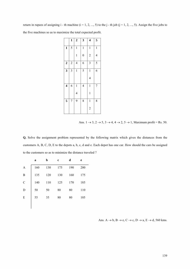
return in rupees of assigning i - th machine (i = 1, 2, ..., 5) to the j - th job (j = 1, 2, ..., 5). Assign the five jobs to

the five machines so as to maximize the total expected profit.

1 2 3 4 5

1 5 1

1

1

0

1

2

1

4

2 2 4 6 3 5

3 3 1 5 1

4

6

4 6 1

4

4 1

1

7

5 7 9 8 1

2

8

Ans. 1 → 3, 2 → 5, 3 → 4, 4 → 2, 5 → 1, Maximum profit = Rs. 50.

Q. Solve the assignment problem represented by the following matrix which gives the distances from the

customers A, B, C, D, E to the depots a, b, c, d and e. Each depot has one car. How should the cars be assigned

to the customers so as to minimize the distance traveled ?

a b c d e

A 160 130 175 190 200

B 135 120 130 160 175

C 140 110 125 170 185

D 50 50 80 80 110

E 55 35 80 80 105

Ans. A → b, B → e, C → c, D → a, E → d, 560 kms.

139

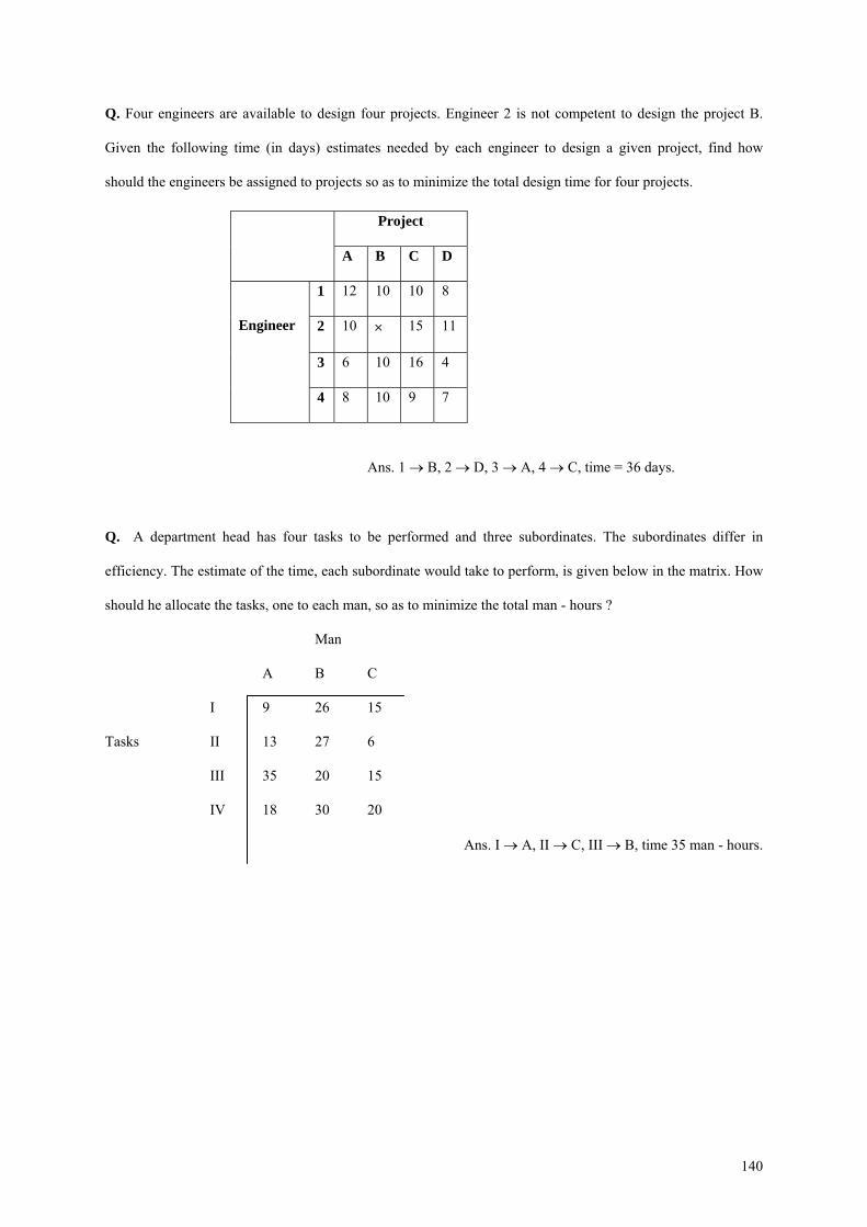
Q. Four engineers are available to design four projects. Engineer 2 is not competent to design the project B.

Given the following time (in days) estimates needed by each engineer to design a given project, find how

should the engineers be assigned to projects so as to minimize the total design time for four projects.

Project

A B C D

1 12 10 10 8

2 10 × 15 11

3 6 10 16 4

Engineer

4 8 10 9 7

Ans. 1 → B, 2 → D, 3 → A, 4 → C, time = 36 days.

Q. A department head has four tasks to be performed and three subordinates. The subordinates differ in

efficiency. The estimate of the time, each subordinate would take to perform, is given below in the matrix. How

should he allocate the tasks, one to each man, so as to minimize the total man - hours ?

Man

A B C

I 9 26 15

Tasks II 13 27 6

III 35 20 15

IV 18 30 20

Ans. I → A, II → C, III → B, time 35 man - hours.

140

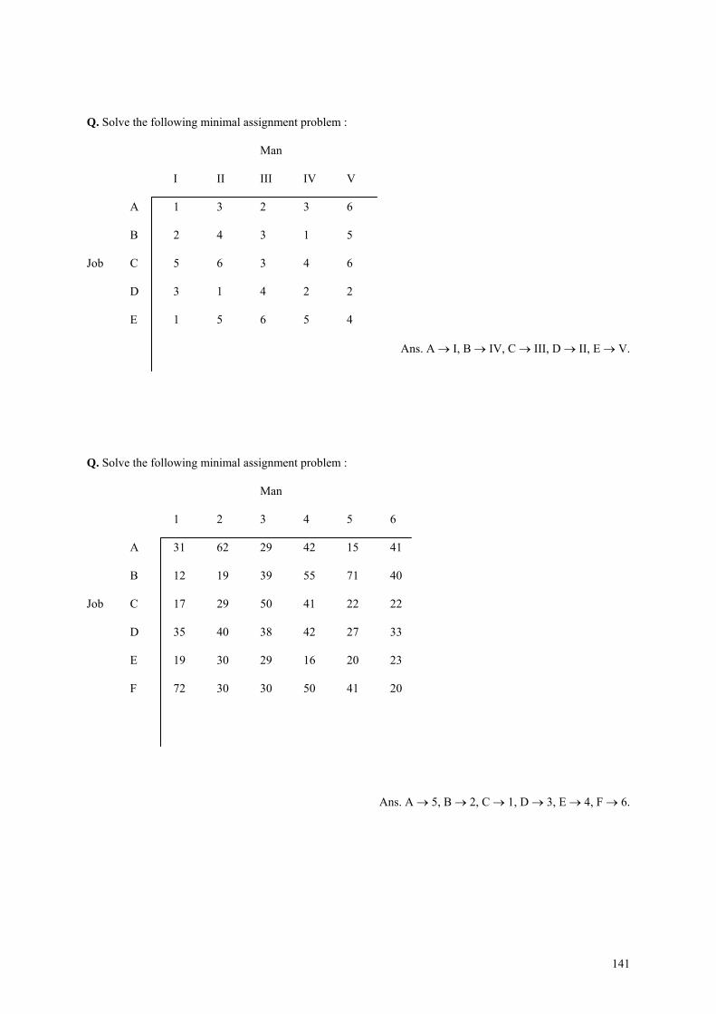
Q. Solve the following minimal assignment problem :

Man

I II III IV V

A 1 3 2 3 6

B 2 4 3 1 5

Job C 5 6 3 4 6

D 3 1 4 2 2

E 1 5 6 5 4

Ans. A → I, B → IV, C → III, D → II, E → V.

Q. Solve the following minimal assignment problem :

Man

1 2 3 4 5 6

A 31 62 29 42 15 41

B 12 19 39 55 71 40

Job C 17 29 50 41 22 22

D 35 40 38 42 27 33

E 19 30 29 16 20 23

F 72 30 30 50 41 20

Ans. A → 5, B → 2, C → 1, D → 3, E → 4, F → 6.

141